Universal Sharpness Dynamics in Neural Network Training:
Fixed Point Analysis, Edge of Stability, and Route to Chaos

Abstract

In gradient descent dynamics of neural networks, the top eigenvalue of the Hessian of the loss (sharpness) displays a variety of robust phenomena throughout training. This includes early time regimes where the sharpness may decrease during early periods of training (sharpness reduction), and later time behavior such as progressive sharpening and edge of stability. We demonstrate that a simple $2$-layer linear network (UV model) trained on a single training example exhibits all of the essential sharpness phenomenology observed in real-world scenarios. By analyzing the structure of dynamical fixed points in function space and the vector field of function updates, we uncover the underlying mechanisms behind these sharpness trends. Our analysis reveals (i) the mechanism behind early sharpness reduction and progressive sharpening, (ii) the required conditions for edge of stability, and (iii) a period-doubling route to chaos on the edge of stability manifold as learning rate is increased. Finally, we demonstrate that various predictions from this simplified model generalize to real-world scenarios and discuss its limitations.

1 Introduction

Over the last several years, it has been observed that the training dynamics of neural networks exhibits a rich and robust set of unexpected phenomena, due to the non-convexity of the loss landscape. Understanding these phenomena may yield insights into the poorly understood nature of the loss landscape and its relationship with model capabilities, and may ultimately lead to improved optimization techniques.

In particular, the unexpected and robust phenomenology is largely associated with the evolution of the Hessian of the loss function, which provides a measure of the local curvature of the loss landscape and which plays an important role in understanding generalization performance (Keskar et al., 2016; Dziugaite & Roy, 2017; Jiang et al., 2019). On the one hand, it has been observed that at late training times, gradient descent (GD) typically exhibits “progressive sharpening,” where the top eigenvalue of the loss Hessian $\lambda^{H}$, which we refer to as the sharpness, gradually increases with time, until it reaches roughly $2/\eta$, where $\eta$ is the learning rate. Once the sharpness reaches roughly $2/\eta$, it stops increasing and typically oscillates near $2/\eta$, a late-time training phenomenon referred to as the “edge of stability (EoS)” regime (Cohen et al., 2021).

On the other hand, at early times, the training dynamics exhibits a different robust set of phenomena, resulting in a phase diagram for early time training dynamics (Kalra & Barkeshli, 2023). As the learning rate is increased, there are regimes where the sharpness decreases quickly before temporarily hitting a plateau (referred to as “sharpness reduction”), and other regimes where the sharpness may suddenly increase within the first few steps of training before quickly dropping and temporarily hitting a plateau (sharpness catapult). Similarly, for large enough learning rates, the training temporarily destabilizes and the network “catapults” out of its local basin, leading to a temporary sudden increase in the loss in the first few steps, before eventually settling down in a flatter region of the loss landscape with lower loss and sharpness (Lewkowycz et al., 2020).

The discovery of the progressive sharpening and EoS regimes and the loss catapult mechanism has attracted significant attention, with an emphasis on various toy models that exhibit similar phenomenology. In this paper, we analyze a popular toy model, a $2$-layer linear network trained on one example, referred to as the UV model. We show that all of the phenomena described above can be observed in the UV model for appropriate choices of learning rate, initialization, parameterization, and choice of training example. Moreover, we show that an analysis of the fixed points, their local stability, and the vector field of updates in function space can give significant insight into the origin of these phenomena. Our analysis of the UV model suggests several non-trivial predictions that we verify in realistic architectures with real and synthetic datasets.

1.1 Our contributions

We revisit the four training regimes identified by Kalra & Barkeshli (2023) (early time transient, intermediate saturation, progressive sharpening, and late time EoS) in Section 3, with a focus on the role of initializations and parameterizations. Our findings reveal that models in Standard Parameterization (SP) with large initializations do not exhibit EoS, even at late training times. Moreover, we show that models in Maximal Update Parameterization ($\mu$P), introduced by Yang & Hu (2021) do not experience an early sharpness reduction. This result also holds for models in SP with small initializations.

We show the UV model exhibits all four training regimes and also captures the effect of initializations and parameterization discussed above. Through fixed-point analysis of the UV model in the function space, we analyze the origins of the various dynamical phenomena exhibited by the sharpness. Specifically, we demonstrate in Sections 4 and 5: (i) the emergence of various sharpness phenomena arising from the stability and position of the dynamical fixed points, (ii) a critical learning rate $\eta_{c}$, above which the model exhibits EoS on a sub-quadratic manifold, and (iii) a period-doubling route to chaos of sharpness fluctuations as a function of learning rate in the EoS regime.

In Section 6, we verify various non-trivial predictions from the UV model in realistic architectures with real and synthetic datasets. Our findings reveal: (i) a sharpness-weight norm correlation before the training enters the EoS regime, (ii) a phase diagram of EoS, revealing that models in $\mu$P and small initialization are more prone to show EoS, and (iii) a period-doubling route to chaos in real architectures trained on synthetic datasets, while those trained on real datasets exhibit long-range correlations at the EoS, with a remnant of the period doubling route to chaos.

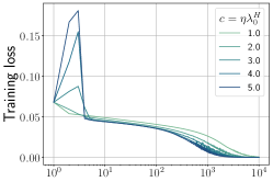
(a)

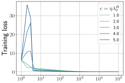
(b)

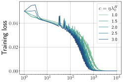
(c)

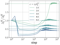
(d)

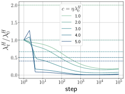
(e)

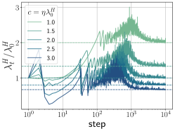
(f)

Figure 1: Training loss and sharpness trajectories of $4$-layer ReLU FCNs with $n=512$, trained on a subset of $5,000$ CIFAR-10 examples using MSE loss and GD: (a, d) SP with $\sigma^{2}_{w}=0.5$, (b, e) SP with $\sigma^{2}_{w}=2.0$, (c, f) $\mu$P with $\sigma^{2}_{w}=2.0$.

1.2 Related works

Sharpness dynamics at large learning rates:
Lewkowycz et al. (2020) examined the early training dynamics of wide networks at large learning rates. Using the top eigenvalue of the Neural Tangent Kernel (NTK) $\lambda^{K}$ at initialization ($t=0$), they revealed a ‘catapult phase’, $\nicefrac{{2}}{{\lambda_{0}^{K}}}<\eta<\eta_{\mathrm{max}}$, in which training converges despite an initial spike in training loss. Kalra & Barkeshli (2023) analyzed early training dynamics for arbitrary depths and width and revealed a ‘sharpness reduction phase’, $\nicefrac{{2}}{{\lambda^{H}_{0}}}<\eta<\nicefrac{{c_{\text{loss}}}}{{\lambda_{0}^{H}}}$, which opens up significantly as $c_{\text{loss}}$ increases with depth and $\nicefrac{{1}}{{}}$width. This work further improves the understanding of the early training dynamics by examining the impact of initialization and parameterization.

Beyond early training, sharpness continues to increase, until it reaches a break-even point (Jastrzebski et al., 2020), beyond which GD dynamics typically enters the EoS regime (Cohen et al., 2021). This has motivated various theoretical studies to understand GD dynamics at large learning rates: (Arora et al., 2022; Rosca et al., 2023; Zhu et al., 2023b; Wu et al., 2023; Chen & Bruna, 2023; Ahn et al., 2022a; Kreisler et al., 2023; Song & Yun, 2023; Chen et al., 2023). In particular, Ma et al. (2022) showed that loss functions with sub-quadratic growth exhibit EoS behavior; Wang et al. (2022b) analyzed EoS in a $2$-layer linear network using the norm of the last layer by assuming progressive sharpening. Using the NTK as a proxy for sharpness, Agarwala et al. (2022) demonstrated that a variant of the quadratic model exhibits progressive sharpening and EoS behavior. Damian et al. (2023) assumed a negative correlation between the gradient direction and the top eigenvector of Hessian to show that GD dynamics enters a stable cycle in the EoS regime. Various theoretical studies analyzing these sharpness phenomena rely on strong assumptions, which do not hold in practice or are challenging to verify in realistic settings. By comparison, our analysis of the UV model offers a translation of findings and insights into realistic settings. For a comprehensive discussion of related works, see Appendix A.

2 Mathematical setup

Consider a discrete dynamical system described by $\bm{\theta}_{t+1}=M(\bm{\theta}_{t})$. A fixed point $\bm{\theta}^{*}$ of the dynamics satisfies $M(\bm{\theta}^{*})=\bm{\theta}^{*}$. The linear stability of a fixed point $\bm{\theta}^{*}$ is determined by analyzing the eigenvalues $\{\lambda_{i}^{J^{*}}\}$ of the Jacobian $J_{M}(\bm{\theta}^{*})\coloneqq\nabla_{\bm{\theta}}M(\bm{\theta})\left.\right|_{\bm{\theta}=\bm{\theta}^{*}}$. An eigendirection $\bm{u}_{i}^{J^{*}}$ of a fixed point $\bm{\theta}^{*}$ is stable if $|\lambda_{i}^{J^{*}}|<1$ and unstable if $|\lambda_{i}^{J^{*}}|>1$ (Ott, 2002). The dynamics is captured by the vector field of updates $G(\bm{\theta})\coloneqq M(\bm{\theta})-\bm{\theta}$. The corresponding unit vector is denoted $\hat{G}(\bm{\theta})\coloneqq\nicefrac{{G(\bm{\bm{\theta}})}}{{\|G(\bm{\bm{\theta}})\|}}$.

The UV model refers to a $2$-layer linear network $f:\mathbb{R}^{d}\to\mathbb{R}$ trained on a single example. We parameterize $f$ as $f(\bm{x};\theta)=\frac{1}{\sqrt{n^{1-p}}}\bm{v}^{T}U\bm{x}$, where $\bm{x}\in\mathbb{R}^{d}$ is the input, $n$ is the network width, and $\bm{v}\in\mathbb{R}^{n},U\in\mathbb{R}^{n\times d}$ are trainable parameters, with each component drawn i.i.d. at initialization from a normal distribution $\mathcal{N}(0,\sigma_{w}^{2}/n^{p})$. Here, $p\in[0,1]$ is a parameter that interpolates between NTP and $\mu$P, and $n_{\text{eff}}\coloneqq n^{1-p}$ is referred to as the effective width. We consider the network trained on a single training example $(\bm{x},y)$ using MSE loss $\ell\left(f(\bm{x};\theta),y\right)=\frac{1}{2}\left(f(\bm{x};\theta)-y\right)^{2}$.

3 Review of the four regimes of training

Typical training trajectories of neural networks can be categorized into four training regimes (Kalra & Barkeshli, 2023), as shown in Figure 1(a, d):

• Early time transient: This corresponds to the first few steps of training. At small learning rates ($\eta<\nicefrac{{c_{\text{loss}}}}{{\lambda^{H}_{0}}}$), loss and sharpness decrease monotonically. At larger learning rates ($\eta>\nicefrac{{c_{\text{loss}}}}{{\lambda_{0}^{H}}}$), training catapults out of the initial basin, temporarily increasing the loss, and finally converges to a flatter region (Lewkowycz et al., 2020). By the end of this regime, sharpness has decreased from initialization for all learning rates, and more substantially at larger learning rates. A rich phase diagram, including a sharpness catapult effect, can be mapped out (Kalra & Barkeshli, 2023).

• Intermediate saturation: Following the initial transient regime, sharpness approximately plateaus before gradually increasing.

• Progressive sharpening: In this regime, sharpness continues to increase until it reaches $\lambda^{H}\approx\nicefrac{{2}}{{\eta}}$ (Jastrzebski et al., 2020; Cohen et al., 2021). At large effective widths or small learning rates, training may conclude before reaching this threshold.

• Late-time dynamics (EoS): After progressive sharpening, for MSE loss, sharpness oscillates around $\nicefrac{{2}}{{\eta}}$. For cross-entropy loss, the sharpness oscillates when reaching approximately $\nicefrac{{2}}{{\eta}}$, while decreasing over longer time scales (Cohen et al., 2021).

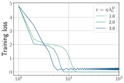
(a)

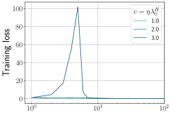
(b)

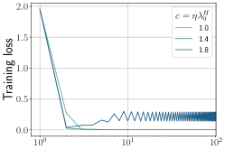
(c)

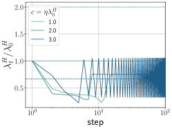
(d)

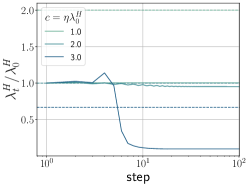
(e)

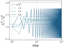
(f)

Figure 2: Training trajectories of the UV model trained on a single example with $\|\bm{x}\|=1$ and $y=2$ using MSE loss and GD: (a, d) NTP with $n=1$, $\sigma^{2}_{w}=0.5$, (b, e) NTP with $n=512$, $\sigma^{2}_{w}=1.0$, and (c, f) $\mu$P with $n=512$, $\sigma^{2}_{w}=1.0$.

Not every training trajectory shows all four training regimes. For instance, Figure 1(b, e) shows that FCNs with large initialization (or large effective width) do not exhibit EoS, even after $10^{5}$ training steps. Following the early transient regime, sharpness monotonically decreases, with only a nominal increase towards late training. Figure 1(c, f) shows that FCNs with small effective widths (or small initializations) do not experience an initial sharpness reduction at small learning rates ($\eta<\nicefrac{{c_{\text{loss}}}}{{\lambda_{0}^{H}}}$). Rather, sharpness continues to increase until it reaches $\nicefrac{{2}}{{\eta}}$ and then oscillates around it. At large learning rates ($\eta>\nicefrac{{c_{\text{sharp}}}}{{\lambda_{0}^{H}}}$), sharpness catapults and eventually settles into the same trend as above.

Figure 2 demonstrates that a $2$-layer linear network, even when trained on a single example (referred to as the UV model), displays all four training regimes. It also captures the cases where sharpness reduction or EoS is not observed. This suggests that this simplified model may serve as an effective model for understanding these universal behaviors in the sharpness dynamics. In the subsequent section, we perform fixed point analysis of the UV model and probe the origin of these complex phenomena in later sections.

4 Fixed point analysis of the UV model

Under GD, the parameters of the UV model are updated as $U_{t+1}=U_{t}-\eta\frac{\Delta f_{t}\bm{v}_{t}\bm{x}^{T}}{\sqrt{n_{\text{eff}}}}$ , $\bm{v}_{t+1}=\bm{v}_{t}-\eta\frac{\Delta f_{t}U_{t}\bm{x}}{\sqrt{n_{\text{eff}}}}$, where $\eta$ is the learning rate and $\Delta f_{t}\coloneqq f(\bm{x};\theta_{t})-y$ is the residual at training step $t$. In function space, the dynamics can be completely described using the residual $\Delta f_{t}$ and trace of the loss Hessian $\lambda\coloneqq\text{Tr }H=\frac{1}{n_{\text{eff}}}\left(\bm{x}^{T}U^{T}U\bm{x}+\bm{v}^{T}\bm{v}\;\bm{x}^{T}\bm{x}\right)$, which is also the scalar neural tangent kernel in this case.

The function space dynamics of the UV model can be fully described using two coupled non-linear equations:

$$\Delta f_{t+1}=\Delta f_{t}\left(1-\eta\lambda_{t}+\frac{\eta^{2}\|\bm{x}\|^{2}}{n_{\text{eff}}}\Delta f_{t}(\Delta f_{t}+y)\right),$$ (1)

$$\lambda_{t+1}=\lambda_{t}+\frac{\eta\;\|\bm{x}\|^{2}}{n_{\text{eff}}}\Delta f_{t}^{2}\left(\eta\lambda_{t}-4\frac{(\Delta f_{t}+y)}{\Delta f_{t}}\right),$$ (2)

with effectively three parameters: $\eta$, $\nicefrac{{\|\bm{x}\|}}{{\sqrt{n_{\mathrm{eff}}}}}$ and $y$. Note that the above equations also describe the dynamics of a wider class of quadratic models, including the quadratic approximation of a $2$-layer ReLU network trained on a single example (Zhu et al., 2022).

Equations 1 and 2 have four distinct fixed points/lines (referred to as I-IV) as detailed in Table 1. The fixed line I defines a zero-loss line, meaning $\ell=0$ for all points in I; the points in I are stable for $\eta\lambda<2$ and unstable otherwise. Fixed point II at $(-y,0)$ corresponds to the origin in parameter space ($U,{\bf v}=0$) and it is a saddle point of the dynamics for convergent learning rates $\eta$. Both I and II are also fixed points of the GD optimization, i.e., critical points of the loss. The loss Hessian at I is positive definite, while fixed point II is a saddle point in the loss landscape. The remaining two fixed points III and IV are unstable and exist only in function space, representing non-trivial parameter space dynamics that leave the function space dynamics invariant.

For $y=0$, there are only three disconnected fixed points/ lines, as II coincides with the origin, merging with the fixed line I. In this case, $\lambda$ can only decrease with time, as can be seen from Equation 2 with $\eta<\eta_{\text{max}}=4/\lambda_{0}$ (training diverges if $\eta>\eta_{\text{max}}$). As a result, the model does not exhibit progressive sharpness and EoS. Prior works (Lewkowycz et al., 2020; Kalra & Barkeshli, 2023) have specifically analyzed this case for understanding catapult dynamics. Below we focus on the case $y>0$, which allows for $\lambda$ to increase in time and consequently, much richer dynamics.

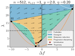
(a)

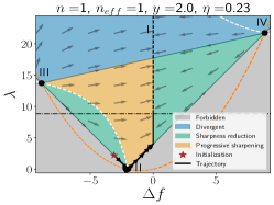
(b)

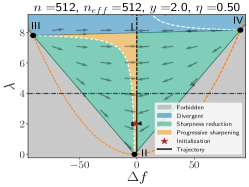
(c)

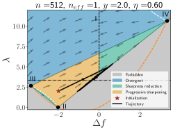
(d)

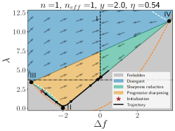
(e)

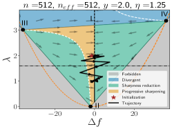
(f)

Figure 3: Training trajectories of the UV model with $\|\bm{x}\|=1$ and $y=2$ in the $(\Delta f,\lambda)$ plane for different values of $n$, $n_{\text{eff}}$ and $\eta$. The columns show initializations with different $n$ and $n_{\text{eff}}$, while the rows represent increasing learning rates for fixed initializations. The horizontal dash-dot line $\eta\lambda=2$ separates the stable (solid black vertical line) and unstable (dashed black vertical line) fixed points along the zero loss fixed line I. Forbidden regions, $2\|\bm{x}\||\Delta f+y|/\sqrt{n_{\text{eff}}}>\lambda$, (see Section C.1) are shaded gray. The nullclines $\Delta f_{t+1}=\Delta f_{t}$ and $\lambda_{t+1}=\lambda_{t}$ are shown as orange and white dashed curves, respectively. Sharpness reduction, progressive sharpening, and divergent regions are colored green, yellow, and blue. The gray arrows indicate the local vector field $\hat{G}(\Delta f,\lambda)$, which is the direction of the updates. The training trajectories are depicted as black lines with arrows, with the star marking the initialization. In all cases, $\eta_{c}=\sqrt{n_{\text{eff}}}/2$ (introduced in Section 5.2).

Figure 3 shows the fixed points and the vector field $\hat{G}(\Delta f,\lambda)$ determined by Equations 1 and 2, which illustrates the direction of the updates at each point. Note that the stability of the fixed line (I) does not follow from $\hat{G}$ alone, as the magnitude $G$ is required to determine stability. Figure 3 also shows training trajectories for various parameter values.

Using $\lambda$ as a proxy for sharpness, we see there are regions where $\lambda$ increases (colored yellow) and decreases (colored green) along the flow, which we refer to as progressive sharpening and sharpness reduction, respectively. It follows from Equation 2 that the condition $\eta\lambda\Delta f=4(\Delta f+y)$ separates these regions. Importantly, the parameters $\eta,\nicefrac{{\|\bm{x}\|}}{{\sqrt{n_{\text{eff}}}}}$ and $y$ influence the position of the fixed points. This, in turn, affects the extent of different regions and the vector field $\hat{G}$, as illustrated in Figure 3. In particular, on decreasing effective width $n_{\text{eff}}$, or increasing learning rate $\eta$, fixed points III and IV move inward (see fixed point expressions in Table 1), which relatively enlarges the progressive sharpening region while shrinking the overall convergent region. Overall, these illustrations demonstrate how the local stability and relative position of the fixed points collectively impact the dynamics. In the subsequent section, we discuss the dynamics in detail.

	$(\Delta f^{*},\lambda^{*})$	Linear stability
I	$(0,\lambda)$ for $\lambda\geq\frac{2\|\bm{x}\|y}{\sqrt{n_{\text{eff}}}}$	$\begin{cases}\text{stable}&\eta\lambda<2\\ \text{unstable}&\eta\lambda>2\end{cases}$
II	$(-y,0)$	saddle
III	$\left(\frac{-2\sqrt{n_{\text{eff}}}}{\|\bm{x}\|\eta},\frac{4}{\eta}-\frac{2\|\bm{x}\|y}{\sqrt{n_{\text{eff}}}}\right)$	unstable
IV	$\left(\frac{2\sqrt{n_{\text{eff}}}}{\|\bm{x}\|\eta},\frac{4}{\eta}+\frac{2\|\bm{x}\|y}{\sqrt{n_{\text{eff}}}}\right)$	unstable

Table 1: Fixed line (I) and points (II-IV) of the update map in Eqs. 1-2. The details of eigenvalues and eigenvectors of the Jacobian are mentioned in Section C.2. The stability is determined for $\eta<\eta_{\mathrm{upper}}=\nicefrac{{2\sqrt{n_{\mathrm{eff}}}}}{{\|\bm{x}\|y}}$. Above this threshold, training diverges for all initializations except for those at the fixed points, as demonstrated in Section C.3.

5 Understanding sharpness dynamics in the UV model

In this section, we describe the origin of different robust phenomena in the dynamics of sharpness using the fixed point and linear stability analysis from the previous section. This explains the four training regimes observed in the UV model. We will discuss the influence of effective width and initializations, shedding light on the differences between NTP and $\mu$P. For simplicity, we assume $\|\bm{x}\|=1$, while allowing $n_{\text{eff}}$ to vary continuously.

Note that we use $\lambda\coloneqq\text{Tr }H$ from the previous section as a proxy for sharpness; we have verified that the top eigenvalue of the Hessian of the loss also follows $\lambda$ (see Section C.4), although it is more difficult to analyze analytically.

5.1 Understanding early and intermediate time sharpness dynamics

Figure 3 shows that the training dynamics can exhibit different behavior depending on the initial region. Below we summarize these based on empirical observations.

• Progressive sharpening region: As shown in Figure 3(a, d), initialization in this region experiences an upward push due to the flow originating from fixed point II, resulting in a steady increase in $\lambda$. Depending on $\eta$ relative to a critical learning rate $\eta_{c}$ (introduced in Section 5.2) different late-time dynamics arises. For $\eta<\eta_{c}$, there exist points on the zero-loss line (I) that are stable, and training always converges to these stable points, as shown in Figure 3(a). When $\eta>\eta_{c}$, all points along the zero-loss line (I) become unstable, as shown in Figure 3(d). In this case, the network eventually converges to a line segment joining fixed points II and IV (the EoS manifold), where it continues to oscillate indefinitely between these fixed points, leading to the EoS phenomena. This will be analyzed in more depth in the subsequent section.

• Sharpness reduction region between fixed points II and III: Figure 3(b, e) show that initializations in this region undergo a decrease in $\lambda$ as the flow is towards saddle point II. On approaching this saddle point, the dynamics slows down, resulting in the intermediate saturation regime observed in Figure 2(a, d). Eventually, training moves away from this saddle and enters the progressive sharpening region. From here on, the dynamics becomes akin to the case (R1).

• Sharpness reduction region b/w fixed line I and point IV: Initializations in this region either converge to the nearby zero-loss solution for ($\eta<\eta_{c}$) or enter the progressive sharpening region for ($\eta>\eta_{c}$). In the latter case, the dynamics resembles those of case (R1).

The model parameterization and width strongly influence the initialization and location of fixed points III and IV, thereby affecting the overall dynamics as discussed below.

Neural Tangent Parameterization: In NTP, $\Delta f$ and $\lambda$ follow normal distributions: $\Delta f_{0}\sim\mathcal{N}(-y,\sigma_{w}^{4})$ and $\lambda_{0}\sim\mathcal{N}(2\sigma_{w}^{2},\nicefrac{{4\sigma_{w}^{4}}}{{n}})$. Hence, the model can be initialized in any of the three regions described above. Moreover, fixed points III and IV move outward with increasing width, affecting the local vector field $\hat{G}(\Delta f,\lambda)$. At large widths $n\gg 1$, $\hat{G}(\Delta f_{0},\lambda_{0})$ at initialization points towards the zero-loss line along $\begin{bmatrix}1&0\end{bmatrix}^{T}$. For small learning rates ($\eta<\nicefrac{{2}}{{\lambda_{0}}}$), training exponentially converges to the nearest zero-loss solution (see Figure 3(c)). Regardless of the initialization region, the change in $\lambda$ is minimal, receiving $\mathcal{O}(\nicefrac{{1}}{{n}})$ updates as per Equation 2. For large learning rates ($\eta>\nicefrac{{2}}{{\lambda_{0}}}$), the nearby zero-loss solution becomes unstable. Consequently, training catapults to a region with smaller $\lambda$, while bouncing between fixed points III and IV. This is the catapult effect studied in (Lewkowycz et al., 2020) and Figure 3(f) demonstrates such a trajectory. By comparison, at small widths, the dynamics follows cases (R1-R3) discussed above.

Maximal Update ($\mu$P) Parameterizations: In contrast to NTP, the position of fixed points III-IV do not change with width $n$, and $\Delta f_{0}$ follows a different distribution: $\Delta f_{0}\sim\mathcal{N}(-y,\nicefrac{{\sigma_{w}^{4}}}{{n}})$, while $\lambda_{0}$ distribution remains unchanged. Consequently, at large widths, the model is initialized at $(-y,2\sigma_{w}^{2})$, right above fixed point II in the progressive sharpening region (R1), satisfying the condition $\eta\lambda_{0}\Delta f_{0}<4(\Delta f_{0}+y)$. Figure 3(a, d) shows such a trajectory. At small widths, fluctuations increase, making it plausible for $\mu$P networks to start in the sharpness reduction regions. In this case, the dynamics follow case (R2) or (R3).

5.2 Understanding Edge of Stability

The origin of the EoS behavior in the UV model arises from the trajectories being attracted to the line segment joining fixed points II and IV (referred to as the EoS manifold), and subsequently oscillating between II and IV along this line, for $\eta>\eta_{c}$.

5.2.1 EoS manifold is a dynamical attractor

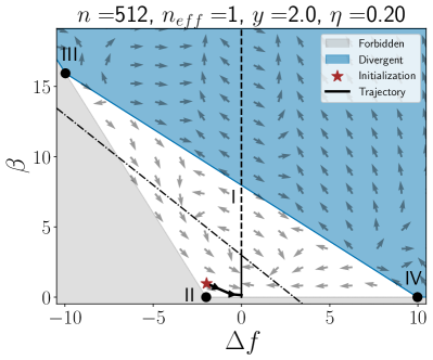
(a)

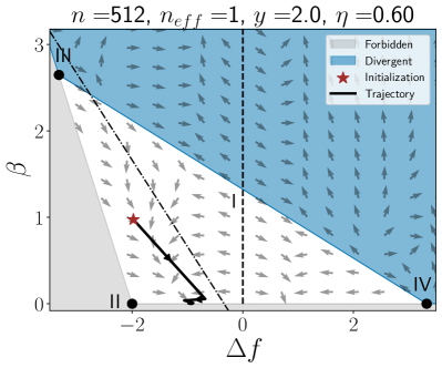
(b)

Figure 4: These plots are equivalent to Figure 3(a, d) ($\eta_{c}=0.5$), but with training trajectory and local vector field plotted for every other step in $(\Delta f,\beta)$ plane. The tilted dash-dotted line indicates the $\eta\lambda=2$ line.

To demonstrate that late time trajectories for $\eta>\eta_{c}$ converge to the EoS manifold, we define $\beta\coloneqq\frac{\sqrt{n_{\text{eff}}}}{2\|\bm{x}\|}\lambda-(\Delta f+y)$. $\beta$ lies on the direction orthogonal to the EoS manifold, such that $\beta=0$ corresponds to the manifold itself, while $\beta<0$ is forbidden. Under this transformation, $\beta$ updates as $\beta_{t+1}=\beta_{t}(1+\frac{\eta\|\bm{x}\|\Delta f_{t}}{\sqrt{n_{\text{eff}}}})^{2}$. It follows that $\beta^{*}=0$ stays invariant under the dynamics and defines a nullcline.

Due to oscillations in $\Delta f$ near convergence, it is instructive to examine the two-step dynamics, compactly denoted as $(\Delta f_{t+2},\lambda_{t+2})\coloneqq M^{(2)}(\Delta f_{t},\lambda_{t})$. Figure 4 shows the two-step trajectories and the corresponding vector field $\hat{G}^{(2)}(\Delta f,\beta)$ in the $(\Delta f,\beta)$ plane.

We observe that there exists a critical $\eta_{c}$ such that for $\eta<\eta_{c}$, $\hat{G}^{(2)}(\Delta f,\beta)$ points towards the stable zero-loss line (see Figure 4(a)). By comparison, for $\eta>\eta_{c}$, all points along the zero-loss line become unstable and the vector field directs towards points on the $\beta=0$ line, as shown in Figure 4(b). The critical $\eta_{c}$ for which all points on the zero-loss line become unstable thus gives a necessary condition for EoS:

Result 1.

Consider the UV model trained on a single example $(\bm{x},y)$ with MSE loss using GD. A necessary condition for EoS is $\eta>\eta_{c}=\frac{\sqrt{n_{\mathrm{eff}}}}{\|\bm{x}\|y}$ (see Section C.6 for details). It is useful to scale the learning rate as $\eta=c/\lambda_{0}$, in which case this condition becomes $\lambda_{0}<\frac{c\|\bm{x}\|y}{\sqrt{n_{\mathrm{eff}}}}$. For learning rates $\eta>2/\lambda_{0}$, training can catapult to regions with $\lambda_{T}<\lambda_{0}$. In such cases, the condition $\lambda_{T}<\frac{c\|\bm{x}\|y}{\sqrt{n_{\mathrm{eff}}}}$ also applies.

5.2.2 Dynamics on the edge of stability manifold and Route to chaos

(a)

(b)

Figure 5: UV model dynamics on the EoS manifold:(a) Bifurcation diagram depicting late-time limiting values of $\lambda$ obtained by simulating Equation 3. (b) Bifurcation diagram of the UV model. In both figures, $\|\bm{x}\|=1,y=2$ and $n_{\text{eff}}$ = 1 and $\eta_{c}=0.5$.

As discussed above, the dynamics on the EoS manifold satisfies $\beta=0$. This corresponds to dynamics along the line $\lambda=\nicefrac{{2\|\bm{x}\|(\Delta f+y)}}{{\sqrt{n_{\text{eff}}}}}$, coupling $\Delta f$ and $\lambda$ together. This yields the map $\Delta f_{t+1}=M_{f}(\Delta f_{t})$ describing the dynamics on the EoS manifold, with $M_{f}$ defined as

$$M_{f}(\Delta f_{t})\coloneqq \Delta f_{t}+\frac{\eta\Delta f_{t}}{\eta_{c}y}\left(\frac{\eta\Delta f_{t}}{\eta_{c}y}-2\right)(\Delta f_{t}+y).$$ (3)

Figure 5(a) shows the limiting values of $\lambda$ (i.e. the values of $\lambda$ that the network jumps between at late times) as a function of learning rate, obtained by simulating Equation 3. We refer to this as the bifurcation diagram. As mentioned above, for $\eta>\eta_{c}$, the zero-loss solution becomes unstable with $\lambda$ oscillating around $\nicefrac{{2}}{{\eta}}$ instead of converging. These fluctuations exhibit a fractal structure, as the system undergoes a series of period-doubling transitions with an increasing learning rate. This is the well-known period-doubling route to chaos (Ott, 2002).

Figure 5(b) shows the bifurcation diagram of the UV model for $y=2$. The bifurcation diagram diagram extends up to $\eta\approx 0.8$ before diverging at higher learning rates. This leads us to the following corollary of Result 1.

Corollary 5.1.

Let $\eta_{\mathrm{max}}$ be the maximum trainable learning rate for a given initialization. Then, the bifurcation diagram is observed up to $\eta<\eta_{\mathrm{max}}$. If $\eta_{\mathrm{max}}<\eta_{c}$, then the UV model does not exhibit EoS behavior.

These results suggest that models with small $\lambda_{0}$ and $n_{\text{eff}}$ are more prone to show EoS behavior. This makes $\mu$P networks or those with small initial weight variance more likely to exhibit EoS. On the other hand, large-width NTP networks would show EoS for small enough $\lambda_{0}$. In the next section, we will validate these findings and earlier predictions in real-world scenarios.

5.2.3 Connections to sub-quadratic loss

(Ma et al., 2022) demonstrated that GD on sub-quadratic loss with large learning rates inherently results in EoS behavior. Here, we show that the loss on the EoS manifold of the UV model is sub-quadratic near its minimum. As noted above, the dynamics on the EoS manifold satisfies $\lambda=\nicefrac{{2\|\bm{x}\|(\Delta f+y)}}{{\sqrt{n_{\text{eff}}}}}$. The loss on the EoS manifold is then given by $\mathcal{L}(\theta)=\frac{1}{2}\Delta f^{2}=\frac{y^{2}}{2}(\frac{\eta_{c}\lambda}{2}-1)^{2}$, where $\theta$ denotes the parameters. Since $\lambda\sim\mathcal{O}(\|\theta\|^{2})$, the loss is of the form $\mathcal{L}(\theta)\approx\frac{1}{2}(a\|\theta\|^{2}-b)^{2}$. This loss is sub-quadratic near its minimum. The GD dynamics near the minimum is given by a cubic map, which is known to show the period-doubling route to chaos (Rogers & Whitley, 1983).

6 Predictions and verifications in real-world scenarios

The preceding analysis offers broader insights and predictions for optimization in real-world models. In this section, we study realistic architectures with real and synthetic datasets and examine the extent to which insights from the UV model generalize.

Experimental setup:

Consider a network ${f}(\bm{x};\theta)$, with trainable parameters $\theta$, initialized using normal distribution with zero mean and variance $\sigma^{2}_{w}$ in appropriate parameterization. Additional details provided in figure captions and Section B.2. The network is trained on a dataset $\mathcal{D}$ with $P$ examples using MSE loss and GD. The learning rate is scaled as $\eta=\nicefrac{{c}}{{\lambda_{0}^{H}}}$, where $c$ is the learning rate constant, and $\lambda_{0}^{H}$ is the sharpness at initialization. In this section, we use the interpolating parameterization with $s\in[0,1]$ (detailed in Section B.2.1), where networks with $s=0$ are equivalent to networks in SP as width $n$ goes to infinity and those with $s=1$ are in $\mu$P.

6.1 Sharpness-Weight norm correlation during training

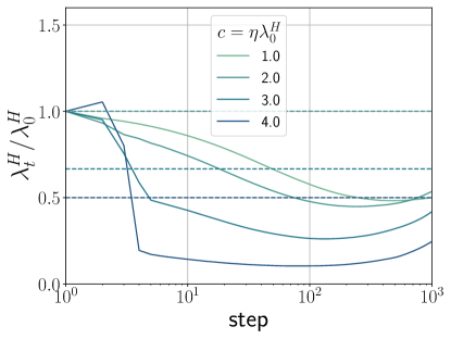
(a)

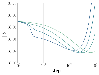
(b)

Figure 6: Sharpness and Weight Norm of $3$-layer ReLU FCNs in SP with $\sigma^{2}_{w}=\nicefrac{{1}}{{3}}$, trained on a subset of CIFAR-10 with $5,000$ examples using GD.

Section 5.1 reveals that several aspects of the training dynamics are controlled by the fact that, for a wide variety of initializations, at early times trajectories move closer to the saddle point II, resulting in an interim decrease in $\lambda$ (also proportional to the weight norm in this case), before eventually increasing. This saddle point where all parameters are zero also exists in real-world models. We thus anticipate that in real-world models, the origin of the four training regimes may be related to a similar mechanism. This would predict a decrease in weight norm as training passes near the saddle point, followed by an eventual increase.

Figure 6 validates this hypothesis. During the sharpness reduction and intermediate saturation regimes, we see a decrease in the weight norm, followed by an increase in the weight norm as the network undergoes progressive sharpening, following the prediction from the UV model. In Appendix E, we provide further evidence for this correlation between sharpness and weight norm, extending this relationship to CNNs and ResNets.

6.2 The phase diagram of edge of stability

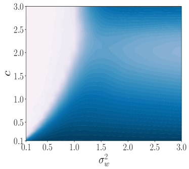
(a)

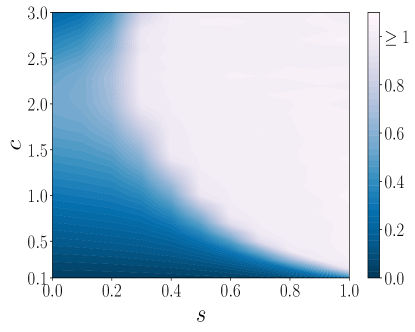
(b)

Figure 7: Phase diagram of EoS: (a) Heatmap of $\nicefrac{{\eta\bar{\lambda}^{H}}}{{2}}$ of $3$-layer ReLU FCNs with $s=0$ trained on a subset of $5,000$ CIFAR-10 examples for 10k steps, with the weight variance $\sigma^{2}_{w}$ and learning rate multiplier $c=\eta\lambda_{0}^{H}$ as axes. $\bar{\lambda}^{H}$ is obtained by averaging $\lambda^{H}_{t}$ over last $200$ steps. As the color varies from blue to white, $\nicefrac{{\eta\bar{\lambda}^{H}}}{{2}}$ increases, where the brightest white region indicates the EoS regime with $\nicefrac{{\eta\bar{\lambda}^{H}}}{{2}}\geq 1$. (b) Same heatmap with fixed $\sigma_{w}^{2}=2.0$, but varying $s$ continuously.

(a)

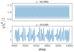
(b)

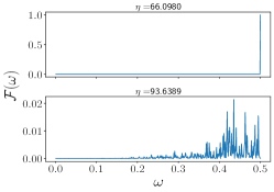
(c)

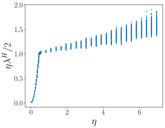
(d)

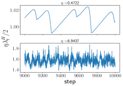
(e)

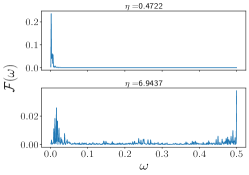
(f)

Figure 8: EoS in random vs real-datasets: $2$-layer linear FCNs trained on (first row) $5,000$ iid random examples with unit output dimension and (second row) $5,000$ CIFAR-10 examples. Different columns correspond to the bifurcation diagram, late-time sharpness trajectories, and the power spectrum of sharpness trajectories. The power spectrum is computed using the last $1000$ steps of the trajectories.

Result 1 presents a necessary condition for EoS to occur in the UV model: $\lambda_{0}<\nicefrac{{c\|\bm{x}\|y}}{{\sqrt{n_{\text{eff}}}}}$. In real-world models, the initial sharpness $\lambda_{0}^{H}$ can be controlled using the initial variance of the weights $\sigma_{w}^{2}$. Therefore, this result predicts that real-world models with (i) small initial weight variance $\sigma^{2}_{w}$, (ii) large interpolating parameter $s$, or (iii) large learning constant $c$ are more likely to exhibit EoS behavior. Figure 7 shows the phase diagram of EoS, validating these predictions. In Appendix F, we illustrate additional phase diagrams for CNNs and ResNets.

6.3 Route to chaos and bifurcation diagrams

The analysis in Section 5.2 unveiled structured fluctuations in $\lambda$ at the EoS, with a period-doubling route to chaos observed as the learning rate is tuned. This motivates us to analyze fluctuations at the EoS in real-world models trained on realistic and synthetic datasets.

Figure 8 shows the bifurcation diagram, late-time sharpness trajectories, and power spectrum of sharpness trajectories for a $2$-layer linear FCN. In the first row, the model is trained on random synthetic data corresponding to $5,000$ iid examples with unit output dimension, whereas, in the second row, on a $5,000$ example subset of CIFAR-10. Similar to the UV model, FCNs trained on random data exhibit a period-doubling route to chaos, as illustrated in Figure 8(a). By comparison, FCNs trained on CIFAR-10 only show dense bands in the sharpness rather than exhibiting a clear period-doubling route to chaos.

On analyzing the sharpness trajectories at EoS, we observe long-range correlations in time in real datasets, with fluctuations increasing with the learning rate (see Figure 8(e)). By comparison, sharpness trajectories of models trained on random datasets exhibit short-period oscillations (see Figure 8(b)). The power spectrum of these sharpness trajectories further quantifies these observations, as shown in Figure 8(c, f). In the random dataset case, high-frequency modes corresponding to the period-doubling route to chaos emerge at EoS as shown in Figure 8(c). In contrast, real datasets exhibit low-frequency modes at small learning rates. As the learning rate is increased, high-frequency modes, reminiscent of the period-doubling route to chaos, start emerging (see Figure 8(f)). In Section G.1, we demonstrate that CNNs and ResNets trained on image datasets show dense bands of sharpness similar to those in FCNs.

To understand when the period-doubling route to chaos arises, we perform further analysis in Appendix G. A key determining feature appears to be whether the singular value spectrum of the input-input and output-input covariance matrices are flat or have power-law decay. In Section G.2, we show that a 2-layer FCNs trained on a random dataset with power-law singular value spectrum in the input exhibits dense sharpness bands. In Section G.3 we show that linear FCNs trained on synthetic datasets with random inputs, such as teacher-student settings and generative settings (details in Section B.1), exhibit the period-doubling route to chaos. In contrast, non-linear networks trained on these tasks exhibit dense sharpness bands as observed in real datasets. These observations shed some light on the nature of EoS observed in realistic settings. Nevertheless, a complete understanding of sharpness fluctuations at EoS requires a separate detailed examination.

7 Discussion

In this work, we performed a fixed-point analysis of the UV model to investigate the underlying mechanisms for various sharpness phenomena observed in real-world scenarios. Importantly, the applicability of this framework extends well beyond the UV model and can be employed in settings involving complex architectures and adaptive optimizers. A prerequisite for applying this method is the closure of the dynamical equations describing the model. By analyzing the fixed points of such equations in broader classes of models, we can gain significant insights into their training dynamics, thereby advancing our understanding of non-convex optimization in neural networks.

Various results such as the phase diagram of EoS, the bifurcation diagram, and the analysis of the late time sharpness trajectories depend on the training time. Nevertheless, we found that training the models longer does not impact the conclusions presented.

In Appendix D, we demonstrate that our results are robust for reasonably small batch sizes ($B\approx 512$). Taking advantage of this, we demonstrate that various presented results apply to CNNs and ResNets. For even smaller batch sizes, the dynamics becomes noise-dominated, and separating the inherent dynamics from noise becomes challenging.

While we focused on models trained with MSE loss, the cross-entropy loss is commonly used in practical settings, which exhibits richer dynamics, especially at late training times. Investigating a minimal model for cross-entropy loss is a promising future direction.

Appendix A Further discussion on related works

Edge of stability:

Ma et al. (2022) show that loss functions with sub-quadratic growth exhibit EoS behavior. Arora et al. (2022) show that normalized gradient descent reaches the EoS regime. Wang et al. (2022b) analyze EoS in a $2$-layer linear network using the norm of the last layer by assuming progressive sharpening. With additional assumptions on the training dataset, they show progressive sharpening in this setup. Damian et al. (2023) analyze the dynamics of the cubic approximation of the loss. Assuming a negative correlation between the gradient direction and the top eigenvector of Hessian, they show that gradient descent dynamics enters a stable cycle in the EoS regime. Using the NTK as a proxy for sharpness, (Agarwala et al., 2022) demonstrated that a variant of the quadratic model exhibits progressive sharpening and EoS behavior.

Zhu et al. (2023b) proved EoS convergence for the loss $\frac{1}{4}(x^{2}y^{2}-1)^{2}$, where $x,y\in\mathbb{R}$. Additionally, they empirically demonstrated a bifurcation diagram in the space of abstract variables of $x$ and $y$. Chen & Bruna (2023) analyze two-step gradient updates of a single-neuron network and matrix factorization to gain insights into EoS. Ahn et al. (2022a) analyze EoS in a single-neuron $2$-layer network and a simplified three-parameter ReLU network assuming the existence of a ‘forward invariant subset’ near the minima.

Wu et al. (2023) demonstrate that gradient descent, with any learning rate in the EoS regime, optimizes logistic regression with linearly separated data over large time scales. Kreisler et al. (2023) analyzed scalar linear networks to show that the sharpness attained by the gradient flow dynamics monotonically decreases in the EoS regime. Rosca et al. (2023) use backward error analysis to incorporate the finite learning rate effect into gradient flow dynamics. Their analysis shows EoS when sharpness is larger than $\nicefrac{{2}}{{\eta}}$, but could not explain progressive sharpening. Song & Yun (2023) analyzed a $2$-layer linear network under logistic loss and demonstrated that sharpness at late training times oscillates around $\nicefrac{{2f}}{{\eta\ell^{\prime}}}$, where $f$ is the network output and $\ell^{\prime}$ is the derivative of the loss. Chen et al. (2023) analyzed large learning rate dynamics of toy models which are characterized by a one-dimensional cubic map and demonstrated five different training phases: (a) monotonic, (b) catapult, (c) periodic, (d) chaotic, and (e) divergent. Wang et al. (2023) categorize training trajectories into three stages: (i) sharpness reduction, (ii) progressive sharpening, and (iii) edge of stability. They argue that different large learning rate behavior depends on the ‘regularity’ of the loss landscape. Specifically, they generalize toy landscapes from existing studies with parameters controlling the regularity. They show that models with good regularity first experience a decrease in sharpness and then progressive sharpening and enter edge of stability.

Parameterizations in neural networks:

Sharpness phenomena in neural networks are intrinsically tied to several factors such as network architecture, depth $d$, width $n$, initialization, and parameterization. Yang & Hu (2021) introduced abc-parametrization that unifies standard parameterization (SP) (Sohl-Dickstein et al., 2020), Neural Tangent Parameterization (NTP) (Jacot et al., 2018) and demonstrate that the two parameterizations are related by a simple transformation in constant width networks. Furthermore, they proposed maximal update parameterization ($\mu$P) (Yang & Hu, 2021), which allows for feature learning as $n\rightarrow\infty$ with $d$ held fixed. Roberts et al. (2022) showed that the leading order features of SP and NTP networks update as $O(\nicefrac{{d}}{{n}})$. Yaida (2022) interpolated between SP and $\mu$P using a parameter $s\in[0,1]$, showing that the leading order features update as $O(\nicefrac{{d}}{{n^{s}}})$.

Appendix B Experimental details

B.1 Datasets

Standard image datasets:

We considered the MNIST (Deng, 2012), Fashion-MNIST (Xiao et al., 2017), and CIFAR-10 (Krizhevsky, 2009) datasets. The images are standardized to have zero mean and unit variance across the feature dimensions, and target labels are represented as one-hot encodings.

Random dataset:

We construct a random dataset $(X,Y)=\{(\bm{x}^{\mu},\bm{y}^{\mu})\}_{\mu=1}^{P}$ with $\bm{x}^{\mu}\sim\mathcal{N}(0,I)$ and $\bm{y}^{\mu}\sim\mathcal{N}(0,I)$, both sampled independently. Note there is no correlation between inputs and outputs.

Teacher-student dataset:

Consider a teacher network ${f}(\bm{x};\theta_{0})$ with $\theta_{0}$ initialized randomly as described in Section B.2. Then, we construct a teacher-student dataset $(X,Y)=\{(\bm{x}^{\mu},\bm{y}^{\mu})\}_{\mu=1}^{P}$ with $\bm{x}^{\mu}\sim\mathcal{N}(0,I)$ and $\bm{y}^{\mu}={f}(\bm{x}^{\mu};\theta_{0})$.

Random power-law dataset:

Starting with the random dataset $(X^{\prime},Y^{\prime})$, we utilize the singular value decomposition of the input and output matrices

$$X^{\prime}=P_{x}S_{x^{\prime}}Q_{x}^{T}, Y^{\prime}=P_{y}S_{y^{\prime}}Q_{y}^{T}.$$ (4)

Next, we rescale the $k^{th}$ singular value of $S_{x^{\prime}}$ and $S_{y^{\prime}}$ as

$$(S_{x})_{k}=A_{x}(S_{x^{\prime}})_{k}k^{-B_{x}} (S_{y})_{k}=A_{y}(S_{y^{\prime}})_{k}k^{-B_{y}},$$ (5)

and re-construct input and output matrices as below

$$X=P_{x}S_{x}Q_{x}^{T}, Y=P_{y}S_{y}Q_{y}^{T}.$$ (6)

The variables $A_{x},B_{x},A_{y}$, and $B_{y}$ uniquely characterize the dataset.

Generative image dataset:

Given a pre-trained network $f(\bm{x};\theta)$ on a standard image dataset listed above, we construct a generative image dataset $(X,Y)=\{(\bm{x}^{\mu},\bm{y}^{\mu})\}_{\mu=1}^{P}$ with $\bm{x}^{\mu}\sim\mathcal{N}(0,I)$ and $\bm{y}^{\mu}=f(\bm{x}^{\mu};\theta)$.

B.2 Models

FCNs:

We considered ReLU FCNs without bias with uniform hidden layer width $n$.

CNNs:

We considered Myrtle family ReLU CNNs (Shankar et al., 2020) without any bias with a fixed number of channels in each layer, which we refer to as the width of the network.

ResNets:

We adapted ResNet (He et al., 2016) implementations from Flax examples. These implementations use Layer norm and initialize the weights as $\mathcal{N}(0,\nicefrac{{\sigma^{2}_{w}}}{{\text{fan}_{\text{in}}}})$. For ResNets, we refer to the number of channels in the first block as the width.

We implemented all models using the JAX (Bradbury et al., 2018), and Flax libraries (Heek et al., 2020).

B.2.1 Details of network parameterization

In this section, we describe different parameterizations used in the paper. For simplicity, we describe the parameterizations for FCNs. Nevertheless, these arguments generalize to other architectures.

Standard Parameterization (SP):

Consider a neural network $f:\mathbb{R}^{d_{\mathrm{in}}}\to\mathbb{R}^{d_{\mathrm{out}}}$ with $d$ layers and constant width $n$. Then, standard parameterization is defined as follows:

$$\bm{h}^{(1)}(\bm{x})=W^{(1)}\bm{x},$$

$$\bm{h}^{(l+1)}(\bm{x})=W^{(l+1)}\phi\left(\bm{h}^{(l)}(\bm{x})\right),$$

$$\bm{f}(\bm{x};\theta)=W^{(d)}\phi\left(\bm{h}^{(d-1)}(\bm{x})\right),$$ (7)

where $W^{(1)}\sim\mathcal{N}(0,\nicefrac{{\sigma^{2}_{w}}}{{d_{\mathrm{in}}}})$, $W^{(l)}\sim\mathcal{N}(0,\nicefrac{{\sigma^{2}_{w}}}{{n}})$ for $1<l<d$, and $W^{(d)}\sim\mathcal{N}(0,\nicefrac{{1}}{{n}})$; $\phi(\cdot)$ is the elementwise activation function. The input is normalized such that $\|\bm{x}\|^{2}=d_{\mathrm{in}}$.

Interpolating Parameterization:

Consider a neural network $f:\mathbb{R}^{d_{\mathrm{in}}}\to\mathbb{R}^{d_{\mathrm{out}}}$ with $d$ layers and constant width $n$. Let $W^{(l)}$ denote the weight matrix at layer $l$. Then, “interpolating parameterization” is defined as follows:

$$\bm{h}^{(1)}(\bm{x})=n^{\nicefrac{{s}}{{2}}}W^{(1)}\bm{x},$$

$$\bm{h}^{(l+1)}(\bm{x})=W^{(l+1)}\phi\left(\bm{h}^{(l)}(\bm{x})\right),$$

$$\bm{f}(\bm{x};\theta)=\frac{1}{n^{\nicefrac{{s}}{{2}}}}W^{(d)}\phi\left(\bm{h}^{(d-1)}(\bm{x})\right),$$ (8)

Here, $s$ is a parameter that interpolates between standard-like parameterization and maximal update parameterization. The weight matrices are sampled from Gaussian distributions: $W^{(1)}\sim\mathcal{N}(0,\nicefrac{{\sigma^{2}_{w}}}{{n^{s}}})$, $W^{(l)}\sim\mathcal{N}(0,\nicefrac{{\sigma^{2}_{w}}}{{n}})$ for $1<l<d$, and $W^{(d)}\sim\mathcal{N}(0,\nicefrac{{1}}{{n}})$. We normalize the input such that $\|\bm{x}\|=1$.

Maximal update Parameterization ($\mu$P):

The maximal update parameterization corresponds to the $s=1$ case in the above setting.

B.3 Details of Figures

Figure 1:

Training loss and sharpness trajectories of $4$-layer ReLU FCNs with $n=512$, trained on a subset of $5,000$ CIFAR-10 examples using MSE loss and GD: (a, d) SP with $\sigma^{2}_{w}=0.5$, (b, e) SP with $\sigma^{2}_{w}=2.0$, (c, f) $\mu P$ with $\sigma^{2}_{w}=2.0$.

Figure 2:

Training trajectories of the UV model trained on a single example with $\|\bm{x}\|=1$ and $y=2$ using MSE loss and GD: (a, d) NTP with $n=1$, $\sigma^{2}_{w}=0.5$, (b, e) NTP with $n=512$, $\sigma^{2}_{w}=1.0$, and (c, f) $\mu$P with $n=512$, $\sigma^{2}_{w}=1.0$.

Figure 3

Training trajectories of the UV model with $\|\bm{x}\|=1$ and $y=2$ in the $(\Delta f,\lambda)$ plane for different values of $n$, $n_{\text{eff}}$ and $\eta$. The columns show initializations with different $n$ and $n_{\text{eff}}$, while the rows represent increasing learning rates for fixed initializations. The horizontal dash-dot line $\eta\lambda=2$ separates the stable (solid black vertical line) and unstable (dashed black vertical line) fixed points along the zero loss fixed line I. Forbidden regions, $2\|\bm{x}\||\Delta f+y|/\sqrt{n_{\text{eff}}}>\lambda$, (see Section C.1) are shaded gray. The nullclines $\Delta f_{t+1}=\Delta f_{t}$ and $\lambda_{t+1}=\lambda_{t}$ are shown as orange and white dashed curves, respectively. Sharpness reduction, progressive sharpening, and divergent regions are colored green, yellow, and blue. The gray arrows indicate the local vector field $\hat{G}(\Delta f,\lambda)$, which is the direction of the updates. The training trajectories are depicted as black lines with arrows, with the star marking the initialization. In all cases, $\eta_{c}=\sqrt{n_{\text{eff}}}/2$ (introduced in Section 5.2).

Figure 4:

Two-step phase portrait of UV model in $(\Delta f,\beta)$ phase plane: These plots are equivalent to Figure 3(d-f), but with training trajectory and local are plotted for every other step.

Figure 5:

UV model dynamics on the EoS manifold:(a) Bifurcation diagram depicting late-time limiting values of $\lambda$ obtained by simulating Equation 3. (b) Bifurcation diagram of the UV model. In both figures, $\|\bm{x}\|=1,y=2$ and $n_{\text{eff}}$ = 1 and $\eta_{c}=0.5$.

Figure 6:

Sharpness and Weight Norm of $3$-layer ReLU FCNs in SP with $\sigma^{2}_{w}=\nicefrac{{1}}{{3}}$, trained on a subset of CIFAR-10 with $5,000$ examples using GD.

Figure 7:

Phase diagram of EoS: (a) Heatmap of $\nicefrac{{\eta\bar{\lambda}^{H}}}{{2}}$ of $3$-layer ReLU FCNs with $s=0$ trained on a subset of $5,000$ CIFAR-10 examples for 10k steps, with the weight variance $\sigma^{2}_{w}$ and learning rate multiplier $c=\eta\lambda_{0}^{H}$ as axes. $\bar{\lambda}^{H}$ is obtained by averaging $\lambda^{H}_{t}$ over last $200$ steps. As the color varies from blue to white, $\nicefrac{{\eta\bar{\lambda}^{H}}}{{2}}$ increases, where the brightest white region indicates the EoS regime with $\nicefrac{{\eta\bar{\lambda}^{H}}}{{2}}\geq 1$. (b) Same heatmap with fixed $\sigma_{w}^{2}=2.0$, but varying $s$ continuously.

Figure 8:

EoS in synthetic vs real-datasets: $2$-layer linear FCN trained on (first row) $5,000$ iid random examples with unit output dimension and (second row) $5,000$ CIFAR-10 examples. Different columns correspond to the bifurcation diagram, late-time sharpness trajectories, and the power spectrum of sharpness trajectories. Both models are trained for $10$k steps using GD.

B.4 Sharpness measurement

We measure sharpness using the power iteration method with $m$ iterations. Typically, $m=20$ iterations ensure convergence. Exceptions requiring more iterates are discussed separately.

B.5 Power spectrum analysis

For a given signal $x^{\prime}(t)$, we standardize the signal

$$x(t)=\frac{x^{\prime}(t)-\mu}{\sigma},$$ (9)

where $\mu$ is the mean and $\sigma^{2}$ is the variance of the signal. Subtracting the mean removes the zero frequency component in the power spectrum. Next, consider the discrete Fourier transform $\mathcal{F}(\omega)$ of $x(t)$:

$$\mathcal{F}(\omega)=\frac{1}{{T}}\sum_{t=0}^{T-1}e^{-\nicefrac{{i2\pi\omega t}}{{T}}}x(t),$$ (10)

Then, the power spectrum is $P(\omega)=|\mathcal{F}(\omega)|^{2}$. The normalization by $T$ in the Fourier transform ensures that the sum of the power spectrum is equal to the variance of the signal, i.e., $\sum_{\omega}P(\omega)=\sigma^{2}$.

Appendix C Properties of the UV model

C.1 Forbidden regions of the UV model

In this section, we utilize the non-negativity of $\lambda$ to derive the condition for allowed regions within the phase plane for the UV model. Consider the function space equations written in terms of the pre-activation $\bm{h}(\bm{x})=U\bm{x}$:

$$f(\bm{x};\theta)=\frac{1}{\sqrt{n_{\text{eff}}}}\bm{v}^{T}\bm{h}(\bm{x})$$ (11)

$$\lambda=\frac{1}{n_{\text{eff}}}\left(\|\bm{v}\|^{2}\|\bm{x}\|^{2}+\|\bm{h}\|^{2}\right).$$ (12)

Let $\cos(\bm{h},\bm{v})$ denote the cosine similarity between $\bm{v}$ and $\bm{h}$. Then, the network output is bounded as

$$|\cos(\bm{h},\bm{v})|=\frac{\sqrt{n_{\text{eff}}}|\Delta f+y|}{\|\bm{v}\|\|\bm{h}\|}\leq 1$$ (13)

Next, using $(\|\bm{v}\|\|\bm{x}\|-\|\bm{h}\|)^{2}\geq 0$, we can bound the product $\|\bm{v}\|\|\bm{h}\|$ using $\lambda$

$$\frac{2\|\bm{x}\|}{\sqrt{n_{\text{eff}}}}|\Delta f+y|\leq\lambda.$$ (14)

The derived inequality describes the allowed phase plane regions for the UV model.

C.2 Fixed Points and Line

	$(\Delta f^{*},\lambda^{*})$	eigenvalues	eigenvectors	Linear stability
I	$(0,\lambda)$ for $\lambda\geq\frac{2\|\bm{x}\|y}{\sqrt{n_{\text{eff}}}}$	$1,1-\eta\lambda$	$\begin{bmatrix}0\\ 1\end{bmatrix},\begin{bmatrix}\frac{n_{\text{eff}}\lambda}{4\|\bm{x}\|^{2}y}\\ 1\end{bmatrix}$	$\begin{cases}\text{stable}&\eta\lambda<2\\ \text{unstable}&\eta\lambda>2\end{cases}$
II	$(-y,0)$	$(1-\frac{\eta\|\bm{x}\|y}{\sqrt{n_{\text{eff}}}})^{2},(1+\frac{\eta\|\bm{x}\|y}{\sqrt{n_{\text{eff}}}})^{2}$	$\begin{bmatrix}-\frac{\sqrt{n_{\text{eff}}}}{2\|\bm{x}\|}\\ 1\end{bmatrix},\begin{bmatrix}\frac{\sqrt{n_{\text{eff}}}}{2\|\bm{x}\|}\\ 1\end{bmatrix}$	saddle
III	$\left(\frac{-2\sqrt{n_{\text{eff}}}}{\|\bm{x}\|\eta},\frac{4}{\eta}-\frac{2\|\bm{x}\|y}{\sqrt{n_{\text{eff}}}}\right)$	$9,5-\frac{2\eta\|\bm{x}\|y}{\sqrt{n_{\text{eff}}}}$	$\begin{bmatrix}\frac{n_{\text{eff}}}{\eta\|\bm{x}\|^{2}y}\\ 1\end{bmatrix},\begin{bmatrix}-\frac{\sqrt{n_{\text{eff}}}}{2\|\bm{x}\|}\\ 1\end{bmatrix}$	unstable
IV	$\left(\frac{2\sqrt{n_{\text{eff}}}}{\|\bm{x}\|\eta},\frac{4}{\eta}+\frac{2\|\bm{x}\|y}{\sqrt{n_{\text{eff}}}}\right)$	$9,5+\frac{2\eta\|\bm{x}\|y}{\sqrt{n_{\text{eff}}}}$	$\begin{bmatrix}\frac{n_{\text{eff}}}{\eta\|\bm{x}\|^{2}y}\\ 1\end{bmatrix},\begin{bmatrix}\frac{\sqrt{n_{\text{eff}}}}{2\|\bm{x}\|}\\ 1\end{bmatrix}$	unstable

Table 2: Fixed line (I) and points (II-IV) and corresponding eigenvalues and eigenvectors of the Jacobian of the update map in Eqs. 1-2. The stability is determined for $\eta<\eta_{\mathrm{upper}}=2\eta_{c}=\nicefrac{{2\sqrt{n_{\mathrm{eff}}}}}{{\|\bm{x}\|y}}$. Above this threshold, training diverges for all initializations except for those at the fixed points, as demonstrated in Section C.3.

Table 2 lists the fixed points of the UV model along with their stability. Additionally, compared to Table 1, it provides the eigenvalues and eigenvectors of the Jacobian for the update maps described by Equations 1 and 2, evaluated at the fixed points.

C.3 The maximum learning rate $\eta_{\text{upper}}$

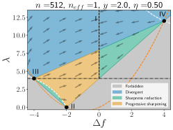
(a)

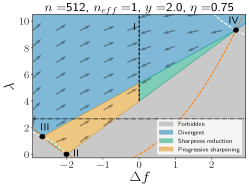
(b)

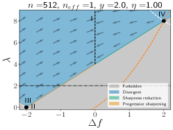
(c)

Figure 9: Phase portrait of the UV model for different learning rates $\eta$. The critical learning rate is $\eta_{c}=0.5$ and the maximum learning rate is $\eta_{\text{upper}}=1.0$.

In Section 4, we stated that for $\eta>\eta_{\text{upper}}=2\eta_{c}$, training diverges for all initializations except for those at the fixed points. Here, we justify this claim.

First, Figure 9 shows that as $\eta$ approaches $\eta_{\text{upper}}$, fixed point III merges with fixed point II, reducing the convergence region to the EoS manifold. At this learning rate, the stability of fixed point II changes from saddle to unstable as the corresponding eigenvalue $(1-\frac{\eta}{\eta_{c}})^{2}\Big{|}_{\eta=2\eta_{c}}$ surpasses $1$. Consequently, any initialization outside the EoS manifold results in divergence. Next, Figure 5(a) shows that on the EoS manifold training diverges for $\eta>\eta_{\text{upper}}$. This corroborates our initial claim.

C.4 Sharpness versus the trace of Hessian

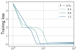
(a)

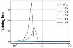
(b)

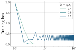
(c)

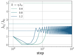
(d)

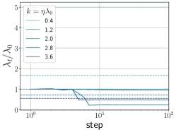
(e)

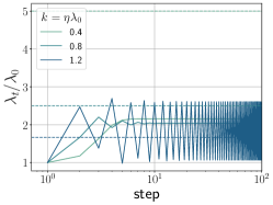
(f)

Figure 10: UV model shows all four training regimes: Training trajectories of the UV model trained on a single example $(\bm{x},y)$ with $\|\bm{x}\|=1$ and $y=2$ using MSE loss and gradient: (a, d) NTP with $n=1$ and $\sigma^{2}_{w}=0.5$ (b, e) NTP with $n=512$ and $\sigma^{2}_{w}=1.0$, and (c, f) $\mu$P with $n=1$ and $\sigma^{2}_{w}=1.0$.

In this section, we show that the trace of the Hessian $\lambda$ (which is also the scalar NTK in this case), is an adequate proxy for sharpness. Figure 10 shows training trajectories of the UV model, with $\lambda$ as a proxy for sharpness and learning rate scaled as $\eta=\nicefrac{{k}}{{\lambda_{0}}}$. These $\lambda$ trajectories show similar trends to those of $\lambda^{H}$ observed in Figure 2, with one key difference: during early training, $\lambda$ does not catapult during early training at large widths (compare Figure 2(e) and Figure 10(e)). Otherwise, $\lambda$ effectively captures other qualitative behavior of $\lambda^{H}$.

C.5 The distribution of residual and NTK at initialization

In this section, we compute the distribution of $\Delta f$ and $\lambda$ for the UV model at initialization. Consider the UV model written in terms of the pre-activation $\bm{h}(\bm{x})=U\bm{x}$,

$$f(\bm{x};\theta)=\frac{1}{\sqrt{n^{1-p}}}\bm{v}^{T}\bm{h}(\bm{x})$$ (15)

$$\lambda=\frac{1}{n^{1-p}}\left(\|\bm{v}\|^{2}\|\bm{x}\|^{2}+\|\bm{h}\|^{2}\right),$$ (16)

with $\bm{v}_{i},U_{ij}\sim\mathcal{N}(0,\nicefrac{{\sigma_{w}^{2}}}{{n^{p}}})$. Then, each pre-activation $h_{i}$ is normally distributed at initialization with zero mean and variance

$$\mathbb{E}_{\theta}[h^{2}_{i}]= \sum_{j,k=1}^{d_{\mathrm{in}}}\langle U_{ij}U_{ik}\rangle x_{j}x_{k}=\sum_{j,k=1}^{d_{\mathrm{in}}}\frac{\sigma_{w}^{2}}{n^{p}}\delta_{jk}x_{j}x_{k}=\frac{\sigma_{w}^{2}\|\bm{x}\|^{2}}{n^{p}}.$$ (17)

Hence, each pre-activation is distributed as $h_{i}\sim\mathcal{N}(0,\nicefrac{{\sigma_{w}^{2}\|\bm{x}\|^{2}}}{{n^{p}}})$. It follows that the network output is also normally distributed at initialization with zero mean and variance

$$\mathbb{E}_{\theta}[f_{0}^{2}]= \frac{1}{n^{1-p}}\sum_{i,j=1}^{n}\langle v_{i}v_{j}\rangle\langle h_{i}h_{j}\rangle=\frac{1}{n^{1-p}}\sum_{i=1}^{n}\frac{\sigma_{w}^{2}}{n^{p}}\frac{\sigma_{w}^{2}\|\bm{x}\|^{2}}{n^{p}}=\frac{\sigma_{w}^{4}\|\bm{x}\|^{2}}{n^{p}}.$$ (18)

Hence, the residual at initialization is distributed as $\Delta f_{0}\sim\mathcal{N}\left(-y,\nicefrac{{\sigma_{w}^{4}\|\bm{x}\|^{2}}}{{n^{p}}}\right)$. Similarly, we can also compute the distribution of $\lambda$ at initialization. The mean value of $\lambda$ is given by

$$\mathbb{E}_{\theta}[\lambda_{0}]=\frac{1}{n^{1-p}}\left(\|\bm{x}\|^{2}\langle\|\bm{v}\|^{2}\rangle+\langle\|\bm{h}\|^{2}\rangle\right)=2\sigma_{w}^{2}\|\bm{x}\|^{2},$$ (19)

where we have used $\langle\|\bm{v}\|^{2}\rangle=\sigma_{w}^{2}n^{1-p}$ and $\langle\|\bm{h}\|^{2}\rangle=\sigma_{w}^{2}\|\bm{x}\|^{2}n^{1-p}$. Using similar computations, the second moment of $\lambda$ is given by:

$$\mathbb{E}_{\theta}[\lambda_{0}^{2}] =\frac{1}{n^{2-2p}}\left(\|\bm{x}\|^{4}\langle\|\bm{v}\|^{4}\rangle+\langle\|\bm{h}\|^{4}\rangle+2\|\bm{x}\|^{2}\langle\|\bm{v}\|^{2}\|\bm{h}\|^{2}\rangle\right)=\frac{4(n+1)}{n}\sigma_{w}^{4}\|\bm{x}\|^{4}\,.$$ (20)

Hence, the $\lambda$ at initialization is distributed as $\lambda_{0}\sim\mathcal{N}\left(2\sigma_{w}^{2}\|\bm{x}\|^{2},\nicefrac{{4\sigma_{w}^{4}\|\bm{x}\|^{4}}}{{n}}\right)$.

C.6 Critical learning rate for edge of stability

In this section, we estimate the required condition on the learning rate for the UV model to exhibit EoS. We specifically focus on the case with $y>0$ as for $y=0$, $\lambda$ can only decrease. As a result, the model does not exhibit progressive sharpening and EoS. In Section 5, we observed that the EoS occurs as the zero-loss minima with the smallest $\lambda$ becomes unstable. From Equation 14 it follows that the smallest $\lambda$ with zero loss is

$$\lambda_{\mathrm{min}}=\frac{2\|\bm{x}\|y}{\sqrt{n_{\text{eff}}}}.$$ (21)

This minimum becomes unstable if the learning rate $\eta$ exceeds a critical value $\eta_{c}$, given by

$$\eta_{c}=\frac{\sqrt{n_{\text{eff}}}}{\|\bm{x}\|y}$$ (22)

It is worth noting that this is a necessary condition for $\lambda$ to oscillate around $\nicefrac{{2}}{{\eta}}$. Otherwise, training converges to the zero-loss minimum with $\lambda=\lambda_{\mathrm{min}}$ for $\eta<\eta_{\mathrm{max}}$.

We can also derive the exact same result by analyzing the dynamics on the EoS manifold. As discussed in Section 5.2, the dynamics on the EoS manifold is given by the map $\Delta f_{t+1}=M(\Delta f_{t})$, where

$$M(\Delta f)=\Delta f\left(1-\frac{2\eta{\|\bm{x}\|}}{{\sqrt{n_{\text{eff}}}}}(\Delta f+y)+\left(\frac{\eta{\|\bm{x}\|}}{{\sqrt{n_{\text{eff}}}}}\right)^{2}\Delta f(\Delta f+y)\right).$$ (23)

As demonstrated in Section 5.2, EoS in the UV model follows the period doubling route to chaos, with the period two cycle marking the onset. Hence, the conditions required for emergence of the period two cycle are also the necessary conditions for EoS. Consider the two-step dynamics on the EoS manifold given by the map $M^{2}(\Delta f)\coloneqq M(M(\Delta f))$. This map has six fixed points (excluding three fixed points of the map $M$) summarized below

$$\Delta f^{*} =\frac{\eta\tilde{x}(1-\eta\tilde{x}y)\pm\sqrt{\eta^{2}\tilde{x}^{2}(\eta\tilde{x}y-1)(3+\eta\tilde{x}y)}}{2\eta^{2}\tilde{x}^{2}}$$ (24)

$$\Delta f^{*} =\frac{3+h(\eta,\tilde{x},y)\pm\eta\tilde{x}(\pm y+\sqrt{2}\sqrt{-\frac{-5+h(\eta,\tilde{x},y)+\eta\tilde{x}y(-2-\eta\tilde{x}y+h(\eta,\tilde{x},y))}{\eta^{2}\tilde{x}^{2}}})}{4\eta\tilde{x}}.$$ (25)

Here $\tilde{x}=\frac{\|\bm{x}\|}{\sqrt{n_{\text{eff}}}}$ and $h(\eta,\tilde{x},y)=\sqrt{-7+\tilde{x}y\eta(2+\tilde{x}y\eta)}$. For the fixed points to exist, we require the expressions inside the square root to be non-negative, i.e.,

$$\left(\frac{\eta\|\bm{x}\|y}{\sqrt{n_{\text{eff}}}}-1\right)\left(\frac{\eta\|\bm{x}\|y}{\sqrt{n_{\text{eff}}}}+3\right)\geq 0\implies\eta\geq\eta_{1}=\frac{\sqrt{n_{\text{eff}}}}{\|\bm{x}\|y}$$ (26)

$$\frac{\eta\|\bm{x}\|y}{\sqrt{n_{\text{eff}}}}\left(\frac{\eta\|\bm{x}\|y}{\sqrt{n_{\text{eff}}}}+2\right)-7\geq 0\implies\eta\geq\eta_{2}=\frac{(\sqrt{32}-2)}{2}\frac{\sqrt{n_{\text{eff}}}}{\|\bm{x}\|y}.$$ (27)

As $\eta_{1}<\eta_{2}$, the necessary condition for the period two cycle to emerge is $\eta>\eta_{1}=\nicefrac{{\sqrt{n_{\text{eff}}}}}{{\|\bm{x}\|y}}$, which coincides with the condition obtained earlier in this section.

Appendix D The effect of batch size on the four training regimes

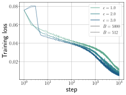
(a)

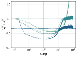
(b)

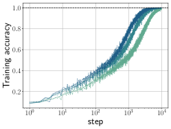
(c)

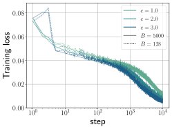
(d)

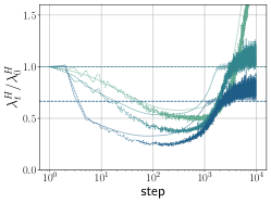
(e)

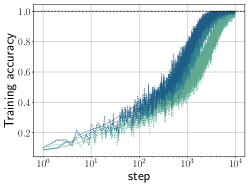
(f)

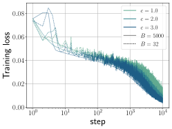
(g)

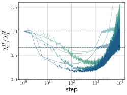
(h)

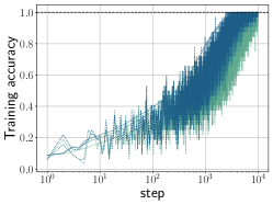
(i)

Figure 11: Comparison of SGD trajectories with their GD counterpart for a $3$-layer FCNs in SP with $\sigma^{2}_{w}=0.5$ trained on a subset of CIFAR-10 consisting of $5,000$ training examples with MSE loss. The learning rate is scaled as $\eta=\nicefrac{{c}}{{\lambda_{0}^{H}}}$ and batch sizes (a-c) $B=512$, (d-f) $B=128$, (g-i) $B=32$ are considered. GD trajectories are plotted using solid lines with transparency.

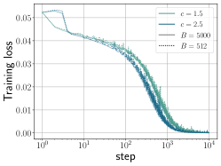
(a)

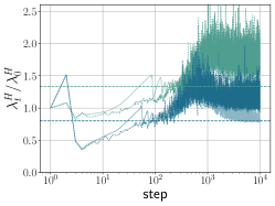
(b)

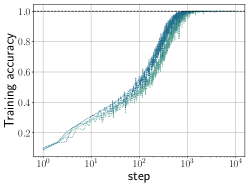
(c)

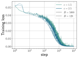
(d)

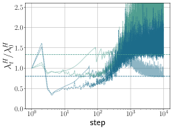
(e)

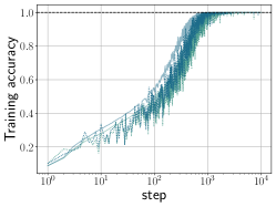
(f)

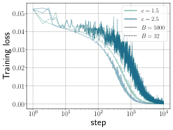
(g)

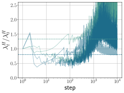
(h)

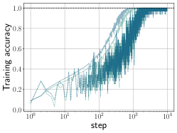
(i)

Figure 12: Same setting as Figure 11, except we used 3-layer FCNs in $\mu$P with $\sigma_{w}^{2}=2.0$.

In this section, we examine the effect of batch size $B$ on the results presented in the main text. We find that our conclusions are robust for reasonable batch sizes around $B\approx 512$. For even smaller batch sizes, the dynamics becomes noise-dominated, and separating the inherent dynamics from noise becomes challenging. This observation further supports the use of SGD to reduce the computational cost of experiments in the subsequent sections involving CNNs and ResNets.

Figure 11 shows that SGD trajectories of FCNs in SP begin to deviate from their GD counterpart significantly for batch sizes around $B\approx 128$. In contrast, for $\mu$P networks this deviation begins at a larger batch size of $B\approx 512$ as shown in Figure 12. Figure 13 show training trajectories of CNNs and ResNets trained SGD with batch size $B=512$. These results further exemplify that four regimes of training are generically observed for reasonable batch sizes.

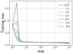
(a)

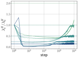
(b)

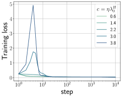
(c)

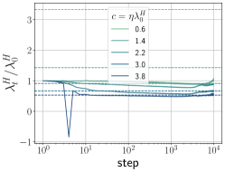
(d)

Figure 13: Training trajectories of (a, b) a $5$-layer CNN in SP with $n=64$, and (c, d) ResNet-18 with LayerNorm in SP, also with $n=64$. Both models are trained on the CIFAR-10 dataset with MSE loss using SGD. The learning rate is scaled as $\eta=\nicefrac{{c}}{{\lambda_{0}^{H}}}$ and batch size is $B=512$. In panel (d), $\lambda^{H}_{t}$ becomes negative during early training. This is due to the power iteration method returning the largest eigenvalue by magnitude.

Appendix E Sharpness-weight norm correlation

This section presents additional results for Section 6.1, further supporting the relationship between sharpness and weight norm during training. Figure 14 shows the weight norm of each layer separately for the experiment in Figure 6. We also confirm these correlations between weight norm and sharpness in CNNs for the experiment in Figure 13(a, b).

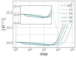
(a)

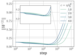
(b)

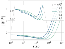
(c)

Figure 14: Weight Norm of each layer in 3-layer ReLU FCNs (same experiments as Figure 6): (a, b, c) SP with $\sigma^{2}_{w}=\nicefrac{{1}}{{3}}$. All results are obtained by training on a subset of CIFAR-10 with $5,000$ examples using GD.

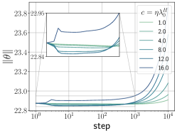
(a)

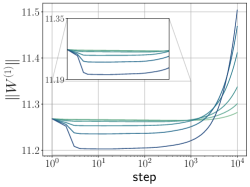
(b)

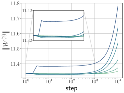
(c)

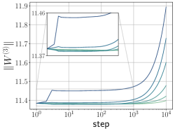
(d)

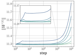
(e)

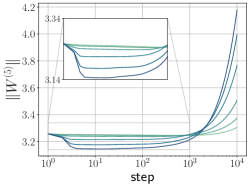
(f)

Figure 15: Weight Norm of each layer for 5-layer CNNs in SP (same experiments as Figure 13(a, b): (a) Total weight norm; (b-f) Weight norm of each layer. We see that for $c=16$, the initial catapult in sharpness $\lambda^{H}$ (Figure 13(b)) is accompanied by a catapult in total weight norm. Notably, the total weight norm and per-layer weight norm, whether catapults (a, c-e) or not (b, f), show a decreasing trend during the early sharpness decreasing stage, followed by an eventual increase, which corroborates our argument in Section 6.1.

Appendix F Additional Phase diagrams of EoS

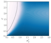
(a)

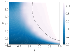
(b)

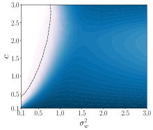
(c)

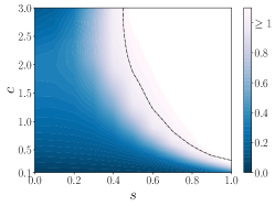
(d)

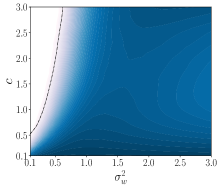
(e)

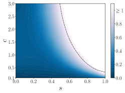
(f)

Figure 16: Phase diagram of EoS for $3$-layer FCNs trained on CIFAR-10 with MSE loss using SGD with three different batch sizes: (a, b) $B=512$, (c, d), $B=128$, and (e, f) $B=32$. The color indicates the value of $\eta\bar{\lambda}^{H}/2$, where $\bar{\lambda}^{H}$ is obtained by averaging $\lambda^{H}_{t}$ over the last 200 steps. Except for the batch size, all settings are identical to Figure 7. Black dash-dotted lines indicate the phase boundary $\eta\bar{\lambda}^{H}/2=1$. For clarity, these lines are generated from data smoothed with a Gaussian kernel.

This section demonstrates additional phase diagrams of EoS and quantifies the effect of batch size in the EoS regime. Figure 16 shows phase diagrams of EoS for FCNs trained on CIFAR-10 with MSE loss using SGD for $10,000$ steps for three different batch sizes. We observe that as the batch size decreases, $\lambda^{H}_{t}$ oscillates at a value different from $\nicefrac{{2}}{{\eta}}$ depending on $\sigma_{w}^{2}$ and $s$. For large $\sigma_{w}^{2}$ and small $s$, $\lambda^{H}$ favors a smaller value for smaller batch size, which is in agreement with the observation in Cohen et al. (2021). In contrast, $\lambda^{H}$ can be larger than $\nicefrac{{2}}{{\eta}}$ for small $\sigma^{2}_{w}$ and large $s$ at late training times.

Figures 17 and 18 show the phase diagrams of EoS for CNNs and ResNets trained on the CIFAR-10 dataset with MSE loss using SGD for $10,000$ steps with learning rate $\eta=\nicefrac{{c}}{{\lambda_{0}^{H}}}$ and batch size $B=512$. In contrast to the FCN phase diagrams, these architectures exhibit EoS behavior at smaller values of $s$ and larger values of $\sigma^{2}_{w}$, indicating their implicit bias towards EoS. Moreover, we observe in ResNets, that EoS is less sensitive to change $\sigma^{2}_{w}$, likely due to a combination of LayerNorm and residual connections (Doshi et al., 2023).

It is worth noting that EoS boundaries in these phase diagrams are time-dependent. For instance, models close to the EoS boundary may eventually reach EoS on training longer (see Figure 13(b) $c=1.0$ for example), causing a shift in the EoS boundary. Nevertheless, models with small learning rates, large $\sigma^{2}_{w}$, and small $s$ may never show EoS behavior, regardless of training duration, as predicted by the UV model and seen in Figure 1(e).

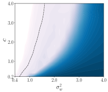
(a)

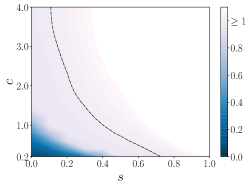
(b)

Figure 17: Phase diagram of EoS for $5$-layer CNNs in SP with width $n=64$ trained with MSE loss using SGD for $10,000$ steps with learning rate $\eta=\nicefrac{{c}}{{\lambda_{0}^{H}}}$ and batch size $B=512$.

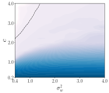
(a)

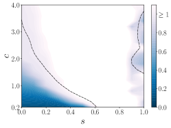
(b)

Figure 18: Phase diagram of EoS for ResNet-18 in SP with width $n=64$ trained with MSE loss using SGD for $10,000$ steps with learning rate $\eta=\nicefrac{{c}}{{\lambda_{0}^{H}}}$ and batch size $B=512$. For $s=1$, the average eigenvalue $\bar{\lambda}^{H}$ is observed to be less than $\nicefrac{{2}}{{\eta}}$. Upon detailed investigation of the trajectories, we found that $\lambda^{H}_{t}$ oscillates around a value lower than $\nicefrac{{2}}{{\eta}}$. We leave this anomalous behavior as an observation.

Appendix G Route to chaos

G.1 Route to EoS in real datasets

This section presents additional bifurcation diagrams for different architectures and datasets. Figures 19, 20 and 21 show the bifurcation diagrams, sharpness trajectories and the associated power spectrum of $4$-layer ReLU FCNs in SP trained on MNIST, Fashion-MNIST and CIFAR-10 datasets with MSE loss using GD. Similarly, Figures 22 and 23 show these results for CNNs and ResNets trained on CIFAR-10 with MSE loss using SGD with batch size $B=512$. These results show the reminiscent of the period-doubling route to chaos observed in different architectures and datasets. In all figures, we choose the smallest and largest learning rate exhibiting EoS for plotting the trajectories and power spectrum. The structured route to chaos in realistic experiments can be disrupted due to a variety of reasons. Below, we discuss a few of them.

Measurement of only the top eigenvalue of Hessian:

In our experiments, we only measured the top eigenvalue of the Hessian. However, when multiple eigenvalues of Hessian enter EoS, plotting only the top eigenvalue of Hessian is a projection that could obscure all the structured routes to chaos that the system may exhibit.

The effect of correlations in real-world datasets:

Real-world datasets inherently contain correlations between different samples ($\bm{x},\bm{y}$). These correlations can be quantified using the input-input covariance matrix $\Sigma_{XX}=XX^{T}\in\mathbb{R}^{d_{\mathrm{in}}\times d_{\mathrm{in}}}$ and output-input covariance matrices $\Sigma_{YX}=YX^{T}\in\mathbb{R}^{d_{\mathrm{out}}\times d_{\mathrm{in}}}$. In Section G.2, we find that a key determining factor in observing route-to-chaos is whether the power spectrum of $\Sigma_{XX}$ is flat or exhibits power law decay. We show that power-law decay in the singular values of the $\Sigma_{XX}$ results in long-range correlations in time and dense sharpness bands observed in real datasets.

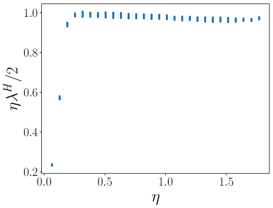
(a)

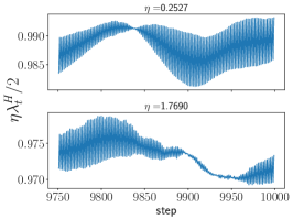
(b)

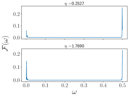
(c)

Figure 19: $4$-layer FCN in SP with width $n=512$ trained on a subset of $5000$ examples of MNIST with MSE loss using GD. Both power spectrums are computed using the last $1000$ steps of the corresponding trajectories.

(a)

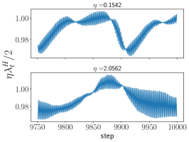
(b)

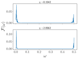
(c)

Figure 20: $4$-layer FCN in SP with width $n=512$ trained on a subset of $5000$ examples of Fashion-MNIST with MSE loss using GD. Both power spectrums are computed using the last $1000$ steps of the corresponding trajectories.

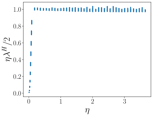
(a)

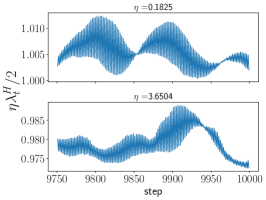
(b)

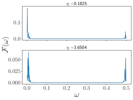
(c)

Figure 21: $4$-layer FCN in SP with width $n=512$ trained on a subset of $5000$ examples of CIFAR-10 with MSE loss using GD. Both power spectrums are computed using the last $1000$ steps of the corresponding trajectories.

(a)

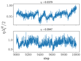
(b)

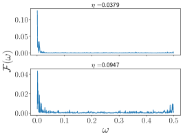
(c)

Figure 22: 5-layer CNN in SP with width $n=64$ trained on a subset of $5000$ examples of CIFAR-10 with MSE loss using SGD with batch size $B=512$.

(a)

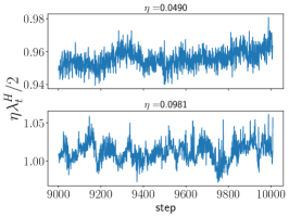
(b)

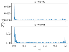
(c)

Figure 23: ResNet-18 in SP with width $n=64$ trained on a subset of $5000$ examples of CIFAR-10 with MSE loss using SGD with batch size $B=512$.

G.2 The effect of power-law trends in data on sharpness trajectories

In this section, we analyze a $2$-layer linear FCN trained on the power law dataset described in Section B.1 to understand the origin of long-range correlations in sharpness trajectories and dense sharpness bands in realistic datasets.

(a)

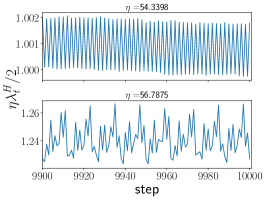
(b)

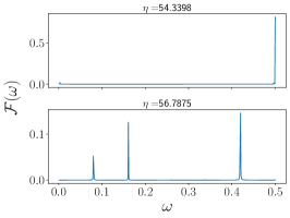
(c)

(d)

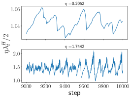
(e)

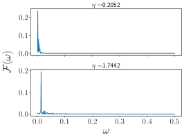
(f)

(g)

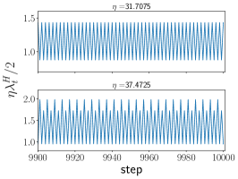
(h)

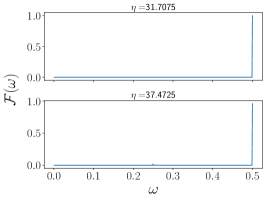
(i)

(j)

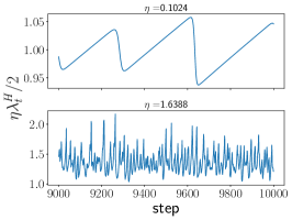
(k)

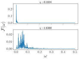
(l)

Figure 24: Bifurcation diagrams, late-time sharpness trajectories, and power spectrum of a $2$-layer linear network trained on the power-law dataset for different parameter values: (a-c) $B_{x}=0.0,B_{y}=0.0$, (d-f) $B_{x}=1.0,B_{y}=0.0$, (g-i) $B_{x}=0.0,B_{y}=1.0$, and (j-l) $B_{x}=1.0,B_{y}=1.0$. All power spectrums are computed using the last $1000$ steps of the corresponding trajectories.

Figure 24 shows the bifurcation diagram, late time trajectories, and the associated power spectrum of the network trained on the power-law dataset with the same $A_{x}=1.0$ and $A_{y}=1.0$, for four different combinations of power-law exponents: (i) $B_{x}=0.0,B_{y}=0.0$, (ii) $B_{x}=1.0,B_{y}=0.0$, (iii) $B_{x}=0.0,B_{y}=1.0$, and (iv) $B_{x}=1.0,B_{y}=1.0$. We observe that a power-law trend to the singular values of the input matrix results in dense sharpness bands observed in real datasets. It is worth noting that this is one way to obtain dense sharpness bands and in general, there can be many other methods.

G.3 Route to chaos in synthetic datasets

In this section, we analyze the route to chaos in synthetic datasets to gain insights into the dense sharpness bands in realistic datasets. We considered two datasets, defined as follows:

Teacher-student dataset:

Consider a teacher FCN $f:\mathbb{R}^{d_{\mathrm{in}}}\to\mathbb{R}^{d_{\mathrm{out}}}$ with $d_{\mathrm{in}}=3072$, $d_{\mathrm{out}}=10$, depth $d$, and width $n=512$ in Standard Paramaterization. Then, we construct a teacher-student dataset $(X,Y)$ consisting of $P=5000$ examples with $\bm{x}^{\mu}\sim\mathcal{N}(0,I)$ and $\bm{y}^{\mu}=\bm{f}(\bm{x}^{\mu};\theta_{0})$. Next, we train a student FCN with the same depth $d$ and depth $n$ as the teacher FCN on this dataset.

(a)

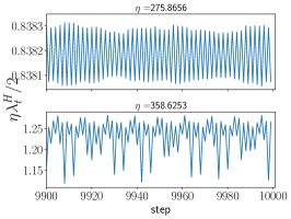
(b)

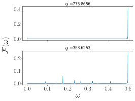
(c)

Figure 25: $2$-layer linear FCN in $\mu$P trained on the teacher-student task. Both power spectrums are computed using the last $1000$ steps of the corresponding trajectories.

(a)

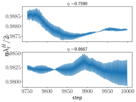
(b)

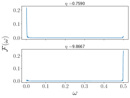
(c)

Figure 26: $4$-layer ReLU FCNs in $\mu$P trained on the teacher-student task. Both power spectrums are computed using the last $1000$ steps of the corresponding trajectories.

Figures 25 and 26 show the bifurcation diagram, late time sharpness trajectories and the associated power spectrum of linear and ReLU FCNs trained on the teacher-student task. These figures show that while linear FCN shows the period-doubling route to chaos, ReLU FCN shows long-range correlations as observed in real datasets.

Generative dataset:

Consider a $5$-layer CNN $\bm{f}(\bm{x},\theta)$ in SP with $n=64$, trained on the CIFAR-10 dataset with MSE loss using SGD with learning rate $\eta=\nicefrac{{12}}{{\lambda_{0}^{H}}}$ and momentum $m=0.9$ for $100$k steps. This model achieves a test accuracy of $76.9\%$. Then, we construct a generative image dataset $(X,Y)$ consisting of $P=5000$ examples with $\bm{x}^{\mu}\sim\mathcal{N}(0,I)$ and $\bm{y}^{\mu}=f(\bm{x}^{\mu};\theta)$. Next, we train an FCN in SP with depth $d$, width $n$, and weight variance $\sigma^{2}_{w}=0.5$ on the generated dataset.

(a)

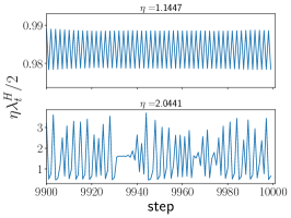
(b)

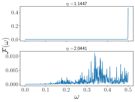
(c)

Figure 27: $4$-layer linear FCNs in SP with $\sigma_{w}^{2}=0.5$ trained on the generative CIFAR-10 task with MSE loss using GD. Both power spectrums are computed using the last $1000$ steps of the corresponding trajectories.

(a)

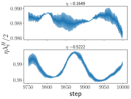
(b)

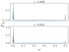
(c)

Figure 28: $4$-layer ReLU FCNs in SP with $\sigma_{w}^{2}=0.5$ trained on the generative CIFAR-10 task with MSE loss using GD. Both power spectrums are computed using the last $1000$ steps of the corresponding trajectories.

Figures 27 and 28 show the bifurcation diagram, late time trajectories and the associated power spectrum of a $4$-layer ReLU FCN with linear and ReLU activations, trained on the generative CIFAR-10 dataset. We observe that while the linear network shows a period doubling route to chaos, the ReLU shows long range correlations as observed in real-datasets.

References

- Agarwala et al. (2022) Agarwala, A., Pedregosa, F., and Pennington, J. A second-order regression model shows edge of stability behavior. In OPT 2022: Optimization for Machine Learning (NeurIPS 2022 Workshop), 2022. URL https://openreview.net/forum?id=A7IpSdqNWHy.
- Ahn et al. (2022a) Ahn, K., Bubeck, S., Chewi, S., Lee, Y. T., Suarez, F., and Zhang, Y. Learning threshold neurons via the ”edge of stability”. ArXiv, abs/2212.07469, 2022a.
- Ahn et al. (2022b) Ahn, K., Zhang, J., and Sra, S. Understanding the unstable convergence of gradient descent. In Chaudhuri, K., Jegelka, S., Song, L., Szepesvari, C., Niu, G., and Sabato, S. (eds.), Proceedings of the 39th International Conference on Machine Learning, volume 162 of Proceedings of Machine Learning Research, pp. 247–257. PMLR, 17–23 Jul 2022b. URL https://proceedings.mlr.press/v162/ahn22a.html.
- Arora et al. (2022) Arora, S., Li, Z., and Panigrahi, A. Understanding gradient descent on the edge of stability in deep learning. In Chaudhuri, K., Jegelka, S., Song, L., Szepesvari, C., Niu, G., and Sabato, S. (eds.), Proceedings of the 39th International Conference on Machine Learning, volume 162 of Proceedings of Machine Learning Research, pp. 948–1024. PMLR, 17–23 Jul 2022. URL https://proceedings.mlr.press/v162/arora22a.html.
- Bai & Lee (2020) Bai, Y. and Lee, J. D. Beyond linearization: On quadratic and higher-order approximation of wide neural networks. In International Conference on Learning Representations, 2020. URL https://openreview.net/forum?id=rkllGyBFPH.
- Bordelon & Pehlevan (2022) Bordelon, B. and Pehlevan, C. Self-consistent dynamical field theory of kernel evolution in wide neural networks. In Advances in Neural Information Processing Systems, 2022. URL https://openreview.net/forum?id=sipwrPCrIS.
- Bordelon & Pehlevan (2023) Bordelon, B. and Pehlevan, C. Dynamics of finite width kernel and prediction fluctuations in mean field neural networks. arXiv, 2304.03408, 2023.
- Bradbury et al. (2018) Bradbury, J., Frostig, R., Hawkins, P., Johnson, M. J., Leary, C., Maclaurin, D., Necula, G., Paszke, A., VanderPlas, J., Wanderman-Milne, S., and Zhang, Q. JAX: composable transformations of Python+NumPy programs, 2018. URL http://github.com/google/jax.
- Chen & Bruna (2023) Chen, L. and Bruna, J. Beyond the edge of stability via two-step gradient updates. arXiv, 2206.04172, 2023.
- Chen et al. (2023) Chen, X., Balasubramanian, K., Ghosal, P., and Agrawalla, B. From stability to chaos: Analyzing gradient descent dynamics in quadratic regression. 2310.01687, 2023.
- Cohen et al. (2021) Cohen, J., Kaur, S., Li, Y., Kolter, J. Z., and Talwalkar, A. Gradient descent on neural networks typically occurs at the edge of stability. In International Conference on Learning Representations, 2021. URL https://openreview.net/forum?id=jh-rTtvkGeM.
- Damian et al. (2023) Damian, A., Nichani, E., and Lee, J. D. Self-stabilization: The implicit bias of gradient descent at the edge of stability. In The Eleventh International Conference on Learning Representations, 2023. URL https://openreview.net/forum?id=nhKHA59gXz.
- Deng (2012) Deng, L. The mnist database of handwritten digit images for machine learning research. IEEE Signal Processing Magazine, 29(6):141–142, 2012.
- Doshi et al. (2023) Doshi, D., He, T., and Gromov, A. Critical initialization of wide and deep neural networks through partial jacobians: General theory and applications. arXiv, 2111.12143, 2023.
- Dziugaite & Roy (2017) Dziugaite, G. K. and Roy, D. M. Computing nonvacuous generalization bounds for deep (stochastic) neural networks with many more parameters than training data. arXiv, 1703.11008, 2017.
- Gilmer et al. (2022) Gilmer, J., Ghorbani, B., Garg, A., Kudugunta, S., Neyshabur, B., Cardoze, D., Dahl, G. E., Nado, Z., and Firat, O. A loss curvature perspective on training instabilities of deep learning models. In International Conference on Learning Representations, 2022. URL https://openreview.net/forum?id=OcKMT-36vUs.
- He et al. (2016) He, K., Zhang, X., Ren, S., and Sun, J. Deep residual learning for image recognition. 2016 IEEE Conference on Computer Vision and Pattern Recognition (CVPR), pp. 770–778, 2016.
- Heek et al. (2020) Heek, J., Levskaya, A., Oliver, A., Ritter, M., Rondepierre, B., Steiner, A., and van Zee, M. Flax: A neural network library and ecosystem for JAX, 2020. URL http://github.com/google/flax.
- Jacot et al. (2018) Jacot, A., Gabriel, F., and Hongler, C. Neural tangent kernel: Convergence and generalization in neural networks. In Bengio, S., Wallach, H., Larochelle, H., Grauman, K., Cesa-Bianchi, N., and Garnett, R. (eds.), Advances in Neural Information Processing Systems, volume 31. Curran Associates, Inc., 2018. URL https://proceedings.neurips.cc/paper_files/paper/2018/file/5a4be1fa34e62bb8a6ec6b91d2462f5a-Paper.pdf.
- Jastrzebski et al. (2020) Jastrzebski, S., Szymczak, M., Fort, S., Arpit, D., Tabor, J., Cho*, K., and Geras*, K. The break-even point on optimization trajectories of deep neural networks. In International Conference on Learning Representations, 2020. URL https://openreview.net/forum?id=r1g87C4KwB.
- Jiang et al. (2019) Jiang, Y., Neyshabur, B., Mobahi, H., Krishnan, D., and Bengio, S. Fantastic generalization measures and where to find them. arXiv, 1912.02178, 2019.
- Kalra & Barkeshli (2023) Kalra, D. S. and Barkeshli, M. Phase diagram of training dynamics in deep neural networks: effect of learning rate, depth, and width. ArXiv, 2302.12250, 2023.
- Keskar et al. (2016) Keskar, N. S., Mudigere, D., Nocedal, J., Smelyanskiy, M., and Tang, P. T. P. On large-batch training for deep learning: Generalization gap and sharp minima. ArXiv, 1609.04836, 2016.
- Kreisler et al. (2023) Kreisler, I., Nacson, M. S., Soudry, D., and Carmon, Y. Gradient descent monotonically decreases the sharpness of gradient flow solutions in scalar networks and beyond. ArXiv, 2305.13064, 2023.
- Krizhevsky (2009) Krizhevsky, A. Learning multiple layers of features from tiny images. 2009.
- Lee et al. (2019) Lee, J., Xiao, L., Schoenholz, S., Bahri, Y., Novak, R., Sohl-Dickstein, J., and Pennington, J. Wide neural networks of any depth evolve as linear models under gradient descent. In Wallach, H., Larochelle, H., Beygelzimer, A., d'Alché-Buc, F., Fox, E., and Garnett, R. (eds.), Advances in Neural Information Processing Systems, volume 32. Curran Associates, Inc., 2019. URL https://proceedings.neurips.cc/paper_files/paper/2019/file/0d1a9651497a38d8b1c3871c84528bd4-Paper.pdf.
- Lewkowycz et al. (2020) Lewkowycz, A., Bahri, Y., Dyer, E., Sohl-Dickstein, J., and Gur-Ari, G. The large learning rate phase of deep learning: the catapult mechanism. ArXiv, 2003.02218, 2020.
- Liu et al. (2023) Liu, C., Huang, W., and Xu, R. Y. D. Implicit bias of deep learning in the large learning rate phase: A data separability perspective. Applied Sciences, 13(6), 2023. ISSN 2076-3417. doi: 10.3390/app13063961. URL https://www.mdpi.com/2076-3417/13/6/3961.
- Ma et al. (2022) Ma, C., Wu, L., and Ying, L. Beyond the quadratic approximation: The multiscale structure of neural network loss landscapes. Journal of Machine Learning, 1(3):247–267, 2022. ISSN 2790-2048. doi: https://doi.org/10.4208/jml.220404. URL http://global-sci.org/intro/article_detail/jml/21028.html.
- Meltzer & Liu (2023) Meltzer, D. and Liu, J. Catapult dynamics and phase transitions in quadratic nets. ArXiv, 2301.07737, 2023.
- Ott (2002) Ott, E. Chaos in Dynamical Systems. Cambridge University Press, 2 edition, 2002. doi: 10.1017/CBO9780511803260.
- Poole et al. (2016) Poole, B., Lahiri, S., Raghu, M., Sohl-Dickstein, J., and Ganguli, S. Exponential expressivity in deep neural networks through transient chaos. In NIPS, 2016.
- Roberts et al. (2022) Roberts, D. A., Yaida, S., and Hanin, B. The Principles of Deep Learning Theory. Cambridge University Press, 2022. https://deeplearningtheory.com.
- Rogers & Whitley (1983) Rogers, T. D. and Whitley, D. C. Chaos in the cubic mapping. Mathematical Modelling, 4(1):9–25, 1983. ISSN 0270-0255. doi: https://doi.org/10.1016/0270-0255(83)90030-1. URL https://www.sciencedirect.com/science/article/pii/0270025583900301.
- Rosca et al. (2023) Rosca, M., Wu, Y., Qin, C., and Dherin, B. On a continuous time model of gradient descent dynamics and instability in deep learning. Transactions on Machine Learning Research, 2023. ISSN 2835-8856. URL https://openreview.net/forum?id=EYrRzKPinA.
- Saxe et al. (2014) Saxe, A. M., McClelland, J. L., and Ganguli, S. Exact solutions to the nonlinear dynamics of learning in deep linear neural networks. arXiv, 1312.6120, 2014.
- Shankar et al. (2020) Shankar, V., Fang, A. W., Guo, W., Fridovich-Keil, S., Schmidt, L., Ragan-Kelley, J., and Recht, B. Neural kernels without tangents. In ICML, 2020.
- Sohl-Dickstein et al. (2020) Sohl-Dickstein, J., Novak, R., Schoenholz, S. S., and Lee, J. On the infinite width limit of neural networks with a standard parameterization. arXiv, 2001.07301, 2020.
- Song & Yun (2023) Song, M. and Yun, C. Trajectory alignment: Understanding the edge of stability phenomenon via bifurcation theory. arXiv, 2307.04204, 2023.
- Strogatz (2000) Strogatz, S. H. Nonlinear Dynamics and Chaos: With Applications to Physics, Biology, Chemistry and Engineering. Westview Press, 2000.
- Wang et al. (2022a) Wang, Y., Chen, M., Zhao, T., and Tao, M. Large learning rate tames homogeneity: Convergence and balancing effect. In International Conference on Learning Representations, 2022a. URL https://openreview.net/forum?id=3tbDrs77LJ5.
- Wang et al. (2023) Wang, Y., Xu, Z., Zhao, T., and Tao, M. Good regularity creates large learning rate implicit biases: edge of stability, balancing, and catapult. arXiv, 2310.17087, 2023.
- Wang et al. (2022b) Wang, Z., Li, Z., and Li, J. Analyzing sharpness along GD trajectory: Progressive sharpening and edge of stability. In Oh, A. H., Agarwal, A., Belgrave, D., and Cho, K. (eds.), Advances in Neural Information Processing Systems, 2022b. URL https://openreview.net/forum?id=thgItcQrJ4y.
- Wu et al. (2023) Wu, J., Braverman, V., and Lee, J. D. Implicit bias of gradient descent for logistic regression at the edge of stability. arXiv, 2305.11788, 2023.
- Xiao et al. (2017) Xiao, H., Rasul, K., and Vollgraf, R. Fashion-mnist: a novel image dataset for benchmarking machine learning algorithms, 2017. URL http://arxiv.org/abs/1708.07747. cite arxiv:1708.07747Comment: Dataset is freely available at https://github.com/zalandoresearch/fashion-mnist Benchmark is available at http://fashion-mnist.s3-website.eu-central-1.amazonaws.com/.
- Yaida (2022) Yaida, S. Meta-principled family of hyperparameter scaling strategies. ArXiv, 2210.04909, 2022.
- Yang & Hu (2021) Yang, G. and Hu, E. J. Tensor programs iv: Feature learning in infinite-width neural networks. In Meila, M. and Zhang, T. (eds.), Proceedings of the 38th International Conference on Machine Learning, volume 139 of Proceedings of Machine Learning Research, pp. 11727–11737. PMLR, 18–24 Jul 2021. URL https://proceedings.mlr.press/v139/yang21c.html.
- Zhu et al. (2022) Zhu, L., Liu, C., Radhakrishnan, A., and Belkin, M. Quadratic models for understanding neural network dynamics. ArXiv, 2205.11787, 2022.
- Zhu et al. (2023a) Zhu, L., Liu, C., Radhakrishnan, A., and Belkin, M. Catapults in sgd: spikes in the training loss and their impact on generalization through feature learning. ArXiv, 2306.04815, 2023a.
- Zhu et al. (2023b) Zhu, X., Wang, Z., Wang, X., Zhou, M., and Ge, R. Understanding edge-of-stability training dynamics with a minimalist example. In The Eleventh International Conference on Learning Representations, 2023b. URL https://openreview.net/forum?id=p7EagBsMAEO.