Closing the Gap to Quadratic Invariance: a Regret Minimization Approach to Optimal Distributed Control

Abstract

In optimal distributed control, state-of-the-art approaches design controllers that comply with an information structure minimizing the $\operatorname*{\mathcal{H}_{2}}2$ or $\operatorname*{\mathcal{H}_{\infty}}$ norm, that is, the expected or worst-case cost in the presence of stochastic or adversarial disturbances. However, performance against the real-world disturbances affecting large-scale systems – which exhibit a complex interplay of stochastic and deterministic elements due to diverse and unmodeled disruptions spreading across the entire system’s scale – remains poor. In this paper, we propose improving performance for these scenarios by minimizing the regret with respect to an ideal policy that complies with less stringent sensor-information constraints. This endows our controller with the ability to approach the improved behavior of a more informed policy, which would detect and counteract heterogeneous and localized disturbances more promptly. Specifically, we derive convex relaxations of the resulting regret minimization problem that are compatible with any desired controller sparsity, while we reveal a renewed role of the Quadratic Invariance (QI) condition in designing informative benchmarks to measure regret. Last, we validate our proposed method through numerical simulations on controlling a large-scale distributed system, comparing its performance with traditional $\operatorname*{\mathcal{H}_{2}}2$ and $\operatorname*{\mathcal{H}_{\infty}}$ policies.

I Introduction

Control of large-scale systems, such as smart grids [1] or traffic systems [2], requires communication among multiple interacting agents to ensure efficient and safe operation. A significant challenge arises from the incomplete information available to each agent regarding the overall system state. This partial communication can be due to various factors, including privacy concerns, geographic dispersion, and the inherent difficulties of establishing a reliable communication network. Designing optimal control policies complying with specific information structures is a well-known challenge, even in seemingly straightforward scenarios, as highlighted by the classic work [3].

The design phase concerning large-scale systems primarily revolves around addressing two fundamental challenges: first, how to parameterize controllers to comply with a given information sparsity, and second, how to formulate a metric that accounts for disturbances and the effect of their propagation throughout the dynamics of the distributed system.

Regarding the first challenge, for linear dynamical systems, a significant breakthrough emerged in the work [4] for the synthesis of sparse linear controllers. The authors introduced the Quadratic Invariance (QI) condition, which has been proved to be both sufficient [4] and necessary [5] for enabling an exact convex reformulation of the aforementioned problem. However, it has been observed that the QI condition can be excessively restrictive regarding its applicability to various systems. To address this issue, [6] introduced communication channels between controllers to effectively restore the QI condition. The works [7, 8] presented convex optimization methods for designing sparse closed-loop dynamics and sparse controllers, even when the QI condition does not hold. In [9, 10] the authors proposed two methods to obtain explicit parametrization of sparse $\operatorname*{\mathcal{H}_{2}}2$ controllers, with [9] considering physically decoupled systems and [10] guaranteeing a control policy behaving similarly to an optimal centralized one, under suitable conditions.

Concerning the second challenge of choosing an appropriate performance metric, traditional control techniques, such as $\operatorname*{\mathcal{H}_{2}}2$ and $\operatorname*{\mathcal{H}_{\infty}}$, often rely on certain assumptions about the nature of disturbances to achieve optimal control policies [11]. $\operatorname*{\mathcal{H}_{2}}2$ treats disturbances as stochastic noise, while $\operatorname*{\mathcal{H}_{\infty}}$ considers them as adversarial attacks. However, these assumptions can be unrealistic and conservative in large-scale scenarios, where disturbances are 1) difficult to model due to the complex dynamics of small local mismatches propagating at large, and 2) difficult to localize, as they may affect agents at unpredictable locations and times. This requires the development of novel control strategies capable of accommodating such non-standard disturbances.

Contributions. To improve the ability of the optimal policy to respond quickly to disturbances with unknown locations and nature, our idea is to close the gap to the performance of an oracle, that is, a benchmark policy that possesses more sensor measurements. By minimizing the worst-case difference in cost with this oracle, our controller design encourages emulation of its behavior, potentially leading to improved performance. This new metric is inspired by the recent works on regret technique [12, 13, 14], which are however limited to centralized control scenarios and focus on a temporal notion of regret.

In this work, we first analyze the conditions for the oracle to express an improved performance to be emulated. We term a spatial regret metric satisfying these capabilities as well-posed. This analysis is achieved by revealing a renewed role of the QI condition within the well-posedness of the proposed metric. Finally, we provide a convex reformulation for designing regret-optimal controllers with arbitrary sparsity structures, optimizing them to close the performance gap to an ideal QI subspace that encodes richer information for the control policy. To illustrate the real-world relevance of our approach, we provide numerical examples involving a multi-agent scenario of a multi-mass spring-damper system that requires to be controlled in the presence of non-standard disturbances.

Structure. The paper is organized as follows. In Section II, we define the problem and introduce the novel spatial regret metric. In Section III, we prove the well-posedness of the spatial regret. Moreover, we formulate the spatial regret optimization problem in a convex form. Lastly, in Section IV we report numerical examples to show the performance of spatial regret in the control of a distributed system.

Notation. The symbol $a\times b$ represents the set of real matrices with dimension $a\times b$. For a matrix $Y\in a\times b$, $Y_{i,j}$ indicates its element in row $i$ and column $j$. Given the vector $x\in a$, $x^{i}$ is used to indicate the $i^{th}$ component of $x$, with $i\in\{1,\dots,a\}$. We denote the set of $a\times b$ binary matrices by $\mathbb{B}^{a\times b}$. Suppose $X\in\mathbb{B}^{a\times b}$ and define the operator

$$\operatorname{Sparse}(X)=\{Y\in a\times b\>|\>Y_{i,j}=0\quad\forall i,j\>\operatorname*{s.t.}\>X_{i,j}=0\}\,.$$

With $\operatorname{card}(X)$ we represent the number of nonzero elements in the binary matrix $X$. For a matrix $Z\in a\times b$, $X=\operatorname{Struct}(Z)\in\mathbb{B}^{a\times b}$ is defined as follows

$$X_{i,j}=\begin{cases}0&\textnormal{ if }Z_{i,j}=0,\\ 1&\textnormal{ otherwise.}\end{cases}\,.$$

For $X,Y\in\mathbb{B}^{a\times b}$, we say $X\leq Y$ if and only if $X_{i,j}\leq Y_{i,j}$, $\forall i,j$. The operators $\left\lVert\cdot\right\rVert_{F}$ and $\left\lVert\cdot\right\rVert_{2\to 2}$ represent the Frobenius and induced 2-norm of a matrix, respectively. Given a symmetric matrix $H\in a\times b$, we denote the largest eigenvalue of H with the symbol $\lambda_{\max}(H)$. Finally, $\mathbf{1}_{T\times T}$ is a $T\times T$ matrix of ones, $\operatorname{Tril}(T)$ is a lower triangular matrix in $\mathbb{B}^{T\times T}$, and the operator $\otimes$ represents the Kronecker product.

II Problem Formulation

We consider discrete-time linear time-varying dynamical systems described by the state-space equations:

$$x_{t+1}=A_{t}x_{t}+B_{t}u_{t}+w_{t}\,,$$ (1)

where $x_{t}\in\mathbb{R}^{n}$, $u_{t}\in\mathbb{R}^{m}$, and $w_{t}\in\mathbb{R}^{n}$ represent the system state, the control input, and an exogenous disturbance, respectively. Motivated by the observation that disturbances affecting large-scale systems often have complex and varied effects on different agents over time, resulting from their high propagation throughout the model dynamics, we want to highlight that we make no assumptions regarding the distribution or the nature of the realizations of $w_{t}$ over time. This approach enables us to address the practical challenges typical of real-world large-scale systems.

We consider the common case where the system described by (1) is controlled over a finite horizon $T\in\mathbb{N}$, starting from an initial condition $x_{0}\in\mathbb{R}^{n}$. For compactness, we represent signals and causal operators over $T$ as

$$\mathbf{x}=\begin{bmatrix}x_{0}\\ x_{1}\\ \vdots\\ x_{T-1}\end{bmatrix}\,,\quad\mathbf{u}=\begin{bmatrix}u_{0}\\ u_{1}\\ \vdots\\ u_{T-1}\end{bmatrix}\,,\quad\bm{\delta}=\begin{bmatrix}x_{0}\\ w_{0}\\ \vdots\\ w_{T-2}\end{bmatrix}=\begin{bmatrix}x_{0}\\ \mathbf{w}\end{bmatrix}\,.$$

At each time instant $t$, we compute the input $u_{t}$ using a causal operator $\pi_{t}$ such that $u_{t}=\pi_{t}(x_{0},\ldots,x_{t})$. For a policy $\bm{\pi}=[\pi_{0}^{\top}(x_{0})\dots\pi_{T-1}^{\top}(x_{0},\dots,x_{T-1})]^{\top}$ and a disturbance $\bm{\delta}$, the incurred cost is defined as

$$J(\bm{\delta},\bm{\pi})=\begin{bmatrix}\mathbf{x}^{\top}&\mathbf{u}^{\top}\end{bmatrix}\mathbf{C}\begin{bmatrix}\mathbf{x}\\ \mathbf{u}\end{bmatrix}\,.$$ (2)

where the matrix $\mathbf{C}\succeq 0$ weights the states and input signals at possibly different time instants. Notice that it is intractable to cast an optimization program over the class of all general policies $\bm{\pi}$. Motivated by their optimality for centralized linear quadratic control and their tractability properties, we focus on linear feedback policies of the form $\mathbf{u}=\mathbf{K}\mathbf{x}\,,$ where $\mathbf{K}\in\mathbb{R}^{mT\times nT}$ is lower block-triangular due to causality. To highlight the dependency of $\mathbf{K}$ in (2), we use from now on the notation $J(\bm{\delta},\mathbf{K})$.

This paper focuses on large-scale systems, where each controller has only access to partial sensor information. We represent this condition using the notation

$$\mathbf{K}\in\mathcal{S}\,,\quad\mathcal{S}=\operatorname{Sparse}(\mathbf{S})\,,$$

where $\mathbf{S}\in\mathbb{B}^{mT\times nT}$ describes the spatio-temporal information of the system, in the sense that $\mathbf{S}$ describes which scalar control input depends on which scalar state, and at which time instant. We will refer to $\mathbf{S}$ as “sparsity matrix”. We assume $\mathbf{S}$ to be lower block-diagonal to guarantee that $\mathbf{K}$ is causal.

II-A Spatial Regret

The cost function (2) depends on the realization of the unknown disturbances $\bm{\delta}$. Hence, finding a sparse controller $\mathbf{K}$ that minimizes (2) for any $\bm{\delta}$ is an ill-posed problem. To remove the explicit dependency of the cost on $\bm{\delta}$, the $\operatorname*{\mathcal{H}_{2}}2$ paradigm optimizes expected performance under the assumption of stochastic disturbances across the entire large-scale system, while the $\operatorname*{\mathcal{H}_{\infty}}$ focuses on optimizing with respect to the worst-case disturbance realization. However, both of these assumptions are unlikely to hold in large-scale systems. The presence of unmodeled dynamics often leads to non-stochastic uncertainties, and disturbances are frequently localized to specific subsystems rather than representing a worst-case scenario. In this paper, we propose an alternative controller performance metric that is tailored to large-scale scenarios.

Suppose, to have an ideal denser sparsity matrix $\mathbf{\hat{S}}$, such that $\mathcal{S}\subset\hat{\mathcal{S}}$, with $\hat{\mathcal{S}}=\operatorname{Sparse}(\mathbf{\hat{S}})$. Then, a controller $\mathbf{\hat{K}}\in\hat{\mathcal{S}}$ would have more sensor information to use, and it would be able to detect and counteract localized disturbances more promptly, regardless of the unknown location where they may hit next. Our idea is to promote the design of sparse controllers that imitate, in hindsight, the behavior of denser ones. To do so, first define the error between the cost of the controller $\mathbf{K}\in{\mathcal{S}}$ and $\mathbf{\hat{K}}\in\hat{\mathcal{S}}$ for a given $\bm{\delta}$ as

$$e(\bm{\delta},\mathbf{K},\mathbf{\hat{K}})=J(\bm{\delta},\mathbf{K})-J(\bm{\delta},\mathbf{\hat{K}})\,.$$ (3)

Then, we introduce a new metric that we denote as “Spatial Regret” quantifying the worst-case scenario of (3) as

$$\operatorname{SpRegret}(\mathbf{K},\mathbf{\hat{K}})=\max_{\lVert\bm{\delta}\rVert_{2}\leq 1}e(\bm{\delta},\mathbf{K},\mathbf{\hat{K}})\,.$$ (4)

Finally, the minimization problem we want to solve is

$$\!\min_{\mathbf{K}} \operatorname{SpRegret}(\mathbf{K},\mathbf{\hat{K}})$$ (5a)

$$~{}\operatorname*{s.t.} \mathbf{K}\in\mathcal{S}\,,\quad\mathcal{S}\subset\hat{\mathcal{S}}\,.$$ (5b)

Problem (5) presents two key challenges. First, we need to verify when the proposed $\operatorname{SpRegret}$ is well-posed, meaning that it remains positive for any selected controller $\mathbf{K}\in\mathcal{S}$, with $\mathbf{\hat{K}}$ chosen properly. Second, notice that (5) is composed of multiple nested optimization problems, making its solution intractable in this form. In Section III-B we provide a convex relaxation of (5) with state-of-the-art tightness.

Remark 1

Our $\operatorname{SpRegret}$ is inspired by [12, 13, 14, 15, 16, 17], which synthesize centralized controllers by minimizing regret with respect to a benchmark policy that has foreknowledge of future realization of $\bm{\delta}$. Unlike these and related works rooted in online optimization, see, e.g., [18], our approach introduces a spatial notion of regret instead of a temporal one. Studying the interplay between spatial and temporal notions of regret is left as an interesting direction for future research.

II-B Review of Convex Design of Distributed Controllers

We review results on the convex design of distributed controllers that are instrumental in solving the challenges depicted above. Let $\mathbf{Z}$ denote the block-downshift operator, namely a matrix with identity matrices along its first block sub-diagonal and zeros elsewhere. Define the matrices $\mathbf{A}=\operatorname{blkdiag}(A_{0},\dots,A_{T-2},0_{n\times n})$, and $\mathbf{B}=\operatorname{blkdiag}(B_{0},\dots,B_{T-2},0_{n\times m})$. Then the state evolution of (1) can be represented compactly as

$$\mathbf{x}=\mathbf{Z}\mathbf{A}\,\mathbf{x}+\mathbf{Z}\mathbf{B}\,\mathbf{u}+\bm{\delta}\,.$$ (6)

Considering a control law $\mathbf{u}=\mathbf{K}\mathbf{x}$ and Eq. (6), it is straightforward to write the closed-loop maps $\bm{\Phi}_{x},\bm{\Phi}_{u}$ from the disturbances $\bm{\delta}$ to $\mathbf{x}$ and $\mathbf{u}$ as

$$\begin{bmatrix}\mathbf{x}\\ \mathbf{u}\end{bmatrix}=\begin{bmatrix}\big{(}I-\mathbf{Z}(\mathbf{A}+\mathbf{B}\mathbf{K})\big{)}^{-1}\\ \mathbf{K}\big{(}I-\mathbf{Z}(\mathbf{A}+\mathbf{B}\mathbf{K})\big{)}^{-1}\end{bmatrix}\bm{\delta}=\begin{bmatrix}\bm{\Phi}_{x}\\ \bm{\Phi}_{u}\end{bmatrix}\bm{\delta}=\mathbf{\Phi}\bm{\delta}.$$ (7)

Here, $\bm{\Phi}$ is the vertical stacking of $\bm{\Phi}_{x},\bm{\Phi}_{u}$. The closed-loop responses $\bm{\Phi}_{x},\bm{\Phi}_{u}$ are lower block-diagonal due to causality. It is easy to verify that $\mathbf{K}$ and $\mathbf{\Phi}$ are linked through the relation $h:(m+n)T\times nT\to mT\times nT$

$$\mathbf{K}=h(\bm{\Phi})=\bm{\Phi}_{u}\bm{\Phi}_{x}^{-1}\,.$$

Also, it can be proved [19] that there exists a controller $\mathbf{K}$ such that (7) holds if and only if

$$(I-\mathbf{Z}\mathbf{A})\bm{\Phi}_{x}-\mathbf{Z}\mathbf{B}\bm{\Phi}_{u}=I\,.$$ (8)

With the introduction of the maps $\bm{\Phi}_{x},\bm{\Phi}_{u}$, the cost $J(\bm{\delta},\mathbf{K})$ can be rewritten as

$$J(\bm{\delta},\mathbf{K})=\bm{\delta}^{\top}\bm{\Phi}^{\top}\mathbf{C}\,\bm{\Phi}\,\bm{\delta}\,.$$ (9)

Moreover, the classic control $\operatorname*{\mathcal{H}_{2}}2$ and $\operatorname*{\mathcal{H}_{\infty}}$ norm, as shown in [19], can be reformulated as

$$\operatorname*{\mathcal{H}_{2}}2:\quad\mathbb{E}_{\bm{\delta}\sim\mathcal{D}}[{J(\bm{\delta},\mathbf{{K}})}]=\left\lVert\mathbf{C}^{\frac{1}{2}}\mathbf{\Phi}\Sigma_{\bm{\delta}}\right\rVert_{F}^{2}\,,$$ (10)

$$\operatorname*{\mathcal{H}_{\infty}}:\quad\max_{\lVert\bm{\delta}\rVert_{2}\leq 1}(J(\bm{\delta},\mathbf{{K}}))=\left\lVert\mathbf{C}^{\frac{1}{2}}\mathbf{\Phi}\right\rVert_{2\to 2}^{2}\,,$$ (11)

where $\mathcal{D}$ in (10) denotes the probability distribution of $\bm{\delta}$, with zero mean and covariance $\Sigma_{\bm{\delta}}\succeq 0$. The costs (10) and (11) become convex in $\mathbf{\Phi}$. Nonetheless, the sparsity condition (5b)

$$\mathbf{K}=h(\mathbf{\Phi})\in\mathcal{S}\,,$$ (12)

becomes nonconvex in $\mathbf{\Phi}$. When the QI condition holds, however, the sparsity constraint (5b) becomes linear in $\mathbf{\Phi}$ [4]. For the sake of clarity, we report its definition.

Definition 1

Define $\mathbf{G}=(I-\mathbf{Z}\mathbf{A})^{-1}\mathbf{Z}\mathbf{B}$. A subspace $\mathcal{S}\subseteq mT\times nT$ is QI with respect to $\mathbf{G}$ if and only if

$$\mathbf{KGK}\in{\mathcal{S}}\,,\quad\forall\mathbf{K}\in{\mathcal{S}}\,.$$

If $\mathcal{S}$ is QI with respect to $\mathbf{G}$, then it is was shown [6] that

$$\mathbf{{K}}\in{\mathcal{S}}\quad\Leftrightarrow\quad\mathbf{{\Phi}}_{u}\Gamma\in{\mathcal{S}}\,,$$ (13)

where $\Gamma=(I-\mathbf{ZA})$. Thus, the QI condition enables to search over all possible sparse controllers $\mathbf{K}\in\mathcal{S}$, allowing globally optimal minimization of any convex cost, such as (10), (11). However, the QI condition may not be satisfied for every desired dynamical system or sparsity matrix. In [8], a technique was introduced for deriving sparse controllers, even in cases where QI does not hold. Specifically, [8] establishes a method to compute, given $\mathcal{S}$, a matrix $V_{x}\in\mathbb{B}^{nT\times nT}$ such that

$$\bm{\Phi}_{u}\Gamma\in\mathcal{S}\quad\textnormal{and}\quad\bm{\Phi}_{x}\Gamma\in\operatorname{Sparse}(V_{x})\,,$$ (14a)

$$\Downarrow$$

$$\mathbf{K}=h(\mathbf{\Phi})=\bm{\Phi}_{u}\bm{\Phi}_{x}^{-1}\in\mathcal{S}\,.$$ (14b)

The authors refer to (14) as Sparsity Invariance (SI) condition. A minimally restrictive choice of the binary matrix $V_{x}$ comply with (14) is given by [Alg. 1][8], which we report below as Algorithm 1 for easier reference.

Algorithm 1 Generation of $V_{x}$ [8, Alg. 1]

1:$\mathbf{S}$ (System’s Sparsity Matrix)

2:Initialize $V_{x}=\mathbf{1}_{nT\times nT}$

3:for each $i=1,\dots,mT$, $k=1,\dots,nT$ do

4:     if $\mathbf{S}_{i,k}==0$ then

5:         for each $j=1,\dots,nT$ do

6:              if $\mathbf{S}_{i,j}==1$ then $(V_{x})_{j,k}\leftarrow 1$              

In this paper, we denote the set of sparse controllers parametrized by SI as

$$\mathbf{\Theta}=\{h(\mathbf{\Phi}):\eqref{eq:achievability_constraint},\>\>\mathbf{\Phi}_{u}\Gamma\in\mathcal{S},\>\>\mathbf{\Phi}_{x}\Gamma\in\operatorname{Sparse}(V_{x})\}\,.$$ (15)

If $V_{x}$ is designed according to Algorithm 1, then we have $\mathbf{\Theta}\subseteq\mathcal{S}$.

III Main Results

Closing the performance gap to a controller $\mathbf{\hat{K}}$ that possesses more sensor measurements does not always lead to improved closed-loop performance. Indeed, a denser controller can perform worse than a sparser one for every realization of disturbances. An example is reported in Section -A. This observation raises the question of how we should design an oracle $\mathbf{\hat{K}}$ so that the optimal $\mathbf{K}^{*}\in\mathcal{S}$ minimizing $\operatorname{SpRegret}(\mathbf{K}^{*},\mathbf{\hat{K}})$ is encouraged to achieve improved performance for non-classical disturbances, or equivalently, $\operatorname{SpRegret}(\mathbf{K}^{*},\mathbf{\hat{K}})\geq 0$. Here, we answer this question in two phases. First, we establish that if the oracle $\mathbf{\hat{K}}\in\hat{\mathcal{S}}$ is optimal according to $\operatorname*{\mathcal{H}_{2}}2$ or $\operatorname*{\mathcal{H}_{\infty}}$ criteria, then $\operatorname{SpRegret}$ is well-posed in the sense that imitating its behavior is advantageous for some $\bm{\delta}$. Second, we interweave this result with the challenge of the convex design of distributed controllers, thus establishing a convex procedure to design denser oracles that are informative by design.

Proposition 1

Assume an oracle $\mathbf{\hat{K}}$ is derived by solving the optimization problem

$$\!\min_{\mathbf{\hat{K}}} f(\mathbf{\hat{K}})$$ (16a)

$$~{}\operatorname*{s.t.} \mathbf{\hat{K}}\in\hat{\mathcal{S}}\,,\quad\mathcal{S}\subset\hat{\mathcal{S}}\,,$$ (16b)

where $f(\mathbf{\hat{K}})$ is $\mathbb{E}_{\bm{\delta}\sim\mathcal{D}}[{J(\bm{\delta},\mathbf{\hat{K}})}]$ or $\max_{\lVert\bm{\delta}\rVert_{2}\leq 1}(J(\bm{\delta},\mathbf{\hat{K}}))$. Then, $\operatorname{SpRegret}(\mathbf{K},\mathbf{\hat{K}})\geq 0$ for any $\mathbf{K}\in\mathcal{S}$.

Proof:

Given $\mathbf{\hat{K}}$ from (16), it always holds that

$$\forall\mathbf{\tilde{K}}\in\hat{\mathcal{S}}\rightarrow\exists\bm{\delta^{*}}:J(\bm{\delta^{*}},\mathbf{\tilde{K}})\geq J(\bm{\delta^{*}},\mathbf{\hat{K}})\,.$$ (17)

This can be proved by contradiction. Indeed, if (17) is false, then

$$\exists\mathbf{\tilde{K}}\in\hat{\mathcal{S}}\rightarrow\forall\bm{\delta}:\,J(\bm{\delta},\mathbf{\tilde{K}})<J(\bm{\delta},\mathbf{\hat{K}})\,.$$

Since the above should hold for every $\bm{\delta}$, then it must also hold for its average realization and worst-case ones, that is, $\mathbb{E}_{\bm{\delta}\sim\mathcal{D}}[{J(\bm{\delta},\mathbf{\tilde{K}})}]<\mathbb{E}_{\bm{\delta}\sim\mathcal{D}}[J(\bm{\delta},\mathbf{\hat{K}})]$, and $\max_{\lVert\bm{\delta}\rVert_{2}\leq 1}(J(\bm{\delta},\mathbf{\tilde{K}}))<\max_{\lVert\bm{\delta}\rVert_{2}\leq 1}(J(\bm{\delta},\mathbf{\hat{K}}))$. This goes against the definition of $\mathbf{\hat{K}}$ from (16), whether obtained minimizing $\mathbb{E}_{\bm{\delta}\sim\mathcal{D}}[J(\bm{\delta},\mathbf{\hat{K}})]$ or $\max_{\lVert\bm{\delta}\rVert_{2}\leq 1}(J(\bm{\delta},\mathbf{\hat{K}}))$. For this reason, (17) must hold. By (17), it follows immediately that

$$\forall\mathbf{K}\in\mathcal{S}\subset\hat{\mathcal{S}}\rightarrow\exists\bm{\delta}:J(\bm{\delta},\mathbf{K})-J(\bm{\delta},\mathbf{\hat{K}})\geq 0\,.$$ (18)

Hence, using definition (4) of spatial regret, (18) shows that $\operatorname{SpRegret}(\mathbf{K},\mathbf{\hat{K}})\geq 0$ for any $\mathbf{K}\in\mathcal{S}$. ∎

Proposition 1 sheds light on two possible design criteria one could follow to synthesize a denser controller $\mathbf{\hat{K}}\in\hat{\mathcal{S}}$ that is guaranteed to be informative, in the sense that no other controller $\mathbf{K}\in\mathcal{S}$ can outperform it for all possible realizations of $\bm{\delta}$. However, up to this point, we have yet to address the convex synthesis of a controller $\mathbf{\hat{K}}$ with sparsity constraints $\mathbf{\hat{S}}$, as required by (16). In the next section of this work, we will delve into this crucial point.

Remark 2

With an unconstrained noncausal benchmark, obtaining an optimal clairvoyant for any $\bm{\delta}$ is possible, as shown in [14, 11]. Therefore, formulations that minimize worst-case regret with a noncausal oracle are always well-posed. Our result in Proposition 1 reaffirms that spatial regret preserves this property even when introducing sparsity constraints in the oracle design.

III-A Synthesis of the Oracle $\mathbf{\hat{K}}$

Thanks to Proposition 1, we have demonstrated there always exist choices for the oracle $\mathbf{\hat{K}}$ that ensure the well-posedness of problem (5). For example, an optimal centralized $\operatorname*{\mathcal{H}_{2}}2$ or $\operatorname*{\mathcal{H}_{\infty}}$ oracle $\mathbf{\hat{K}}$, is a valid choice. However, combining the assurance of well-posedness with the convex reformulations of distributed control synthesis for both $\mathbf{K}$ and $\mathbf{\hat{K}}$ presents a complex challenge. Indeed, to design first $\mathbf{\hat{K}}$ and then $\mathbf{{K}}$, for generic $\mathcal{S}\subset\hat{\mathcal{S}}$, we would be tempted to use for both sparsity constraints the method [8, Alg. 1]. This would return two matrices $V_{x}$, $\hat{V}_{x}$ satisfying the SI condition (14) for $\mathcal{S}$ and $\hat{\mathcal{S}}$, respectively. It must be pointed out that these steps might fail to obtain a well-posed spatial regret metric, in general. An example illustrating this is detailed in Section -B. Nonetheless, in the following Theorem, we reveal the crucial role of the QI condition in designing an informative oracle $\mathbf{\hat{K}}$ in conjunction with SI for the synthesis of the spatial regret optimal policy for any $\mathcal{S}$.

Theorem 1

Let $\hat{\mathcal{S}}$ be QI with respect to $\mathbf{G}$, with ${\mathcal{S}}\subset\hat{\mathcal{S}}$. Additionally, denote with $V_{x}$ and $\hat{V}_{x}$ the binary matrices computed using Algorithm 1 based on ${\mathcal{S}}$ and $\hat{\mathcal{S}}$, respectively. Assume an oracle $\mathbf{\hat{K}}=h(\mathbf{\hat{\Phi}})$ is derived through the optimization problem

$$\min_{\mathbf{\hat{\Phi}}}f(\mathbf{\hat{\Phi}})\>\>\operatorname*{s.t.}\>\eqref{eq:achievability_constraint},\>\>\mathbf{\hat{\Phi}}_{u}\Gamma\in\hat{\mathcal{S}},\>\mathbf{\hat{\Phi}}_{x}\Gamma\in\operatorname{Sparse}(\hat{V}_{x}),$$ (19)

where the function $f(\mathbf{\hat{\Phi}})$ can be either (10) or (11) and $\Gamma=(I-\mathbf{ZA})$. Then, $\operatorname{SpRegret}(\mathbf{K},\mathbf{\hat{K}})\geq 0$ for any $\mathbf{K}\in\mathbf{\Theta}$.

Proof:

The proof follows a two-step process. First, we establish that if $\hat{\mathcal{S}}$ satisfies the QI condition, then it implies $\mathbf{\Theta}\subseteq\mathbf{\hat{\Theta}}$, which are defined as

$$\begin{gathered}\mathbf{\Theta}=\{h(\mathbf{\Phi}):\eqref{eq:achievability_constraint},\>\>\mathbf{\Phi}_{u}\Gamma\in\mathcal{S},\>\>\mathbf{\Phi}_{x}\Gamma\in\operatorname{Sparse}(V_{x})\}\,,\\ \mathbf{\hat{\Theta}}=\{h(\mathbf{\hat{\Phi}}):\eqref{eq:achievability_constraint},\>\>\mathbf{\hat{\Phi}}_{u}\Gamma\in\hat{\mathcal{S}},\>\>\mathbf{\hat{\Phi}}_{x}\Gamma\in\operatorname{Sparse}(\hat{V}_{x})\}\,.\end{gathered}$$ (20)

Second, we demonstrate that the requirements of Proposition 1 are satisfied and $\operatorname{SpRegret}(\mathbf{K},\mathbf{\hat{K}})\geq 0$ for every $\mathbf{K}\in\mathcal{S}$.

We proceed to show that $\mathbf{\Theta}\subseteq\mathbf{\hat{\Theta}}$. Since $\mathcal{S}\subset\hat{\mathcal{S}}$ by construction, then $\mathbf{\Phi}_{u}\Gamma\in\mathcal{S}\Rightarrow\mathbf{\Phi}_{u}\Gamma\in\hat{\mathcal{S}}$. From (8), we can rewrite $\mathbf{\Phi}_{x}$ as

$$\mathbf{\Phi}_{x}=(I-\mathbf{ZA})^{-1}+(I-\mathbf{ZA})^{-1}\mathbf{ZB}\mathbf{\Phi}_{u}\,.$$ (21)

Right-multiplying both sides of (21) by $\Gamma=(I-\mathbf{ZA})$ and using the definition of $\mathbf{G}=(I-\mathbf{ZA})^{-1}\mathbf{ZB}$, we obtain that $\mathbf{\Phi}_{x}\Gamma=I+\mathbf{G}\mathbf{\Phi}_{u}\Gamma$. Moreover, knowing that $\mathbf{G}\in\operatorname{Sparse}(\mathbf{\Delta})$ and $\mathbf{\Phi}_{u}\Gamma\in\operatorname{Sparse}(\mathcal{S})$, then it must hold that $I+\mathbf{G}\mathbf{\Phi}_{u}\Gamma\in\operatorname{Sparse}(I+\mathbf{\Delta}\mathcal{S})$. This means that

$$\mathbf{\Phi}_{x}\Gamma\in\operatorname{Sparse}(I+\mathbf{\Delta}\mathcal{S})\subseteq\operatorname{Sparse}(I+\mathbf{\Delta}\hat{\mathcal{S}})\,.$$

From [8, Th. 4], we know that if $\hat{\mathcal{S}}$ satisfies the QI condition with respect to $\mathbf{G}$, then $\operatorname{Sparse}(I+\mathbf{\Delta}\hat{\mathcal{S}})\subseteq\operatorname{Sparse}(\hat{V}_{x})$, which in turn implies that $\mathbf{\Phi}_{x}\Gamma\in\operatorname{Sparse}(\hat{V}_{x})$. Having established that $\mathbf{\Theta}\subseteq\mathbf{\hat{\Theta}}$, it follows that if a controller $\mathbf{K}\in\mathbf{\Theta}$, then also $\mathbf{K}\in\mathbf{\hat{\Theta}}$.

Regarding the second step of the proof, $\mathbf{\hat{K}}=h(\mathbf{\hat{\Phi}})$ is derived through (19), which is equivalent to solving (16) due to the QI condition. Finally, $\mathbf{\Phi}$ is such that (14a) holds, thus $\mathbf{K}=h(\mathbf{\Phi})\in\mathcal{S}$ thanks to (14) and $\operatorname{SpRegret}(\mathbf{K},\mathbf{\hat{K}})\geq 0$ for Proposition 1. ∎

With Theorem 1, we proved that if the oracle structure satisfies the QI condition, then the well-posedness of the spatial regret metric is preserved using the SI condition (14) to enforce both sparsity constraints over the oracle $\mathbf{\hat{K}}$ and then the actual controller $\mathbf{K}$.

Remark 3

Given the sparsity matrix $\mathbf{S}$, one can obtain its closest QI superset $\mathbf{\hat{S}}_{QI}$ such that

$${\mathbf{\hat{S}}_{QI}}= \operatorname*{argmin}_{\mathbf{S}^{*}} \operatorname{card}(\mathbf{S}^{*}-\mathbf{S})$$ (22)

$$~{}~{}~{}\operatorname*{s.t.} \mathcal{S}\subseteq{\mathcal{S}^{*}},\quad{\mathcal{S}^{*}}=\operatorname{Sparse}(\mathbf{S}^{*}),$$

$$\mathcal{S}^{*}\textnormal{ is QI w.r.t. }\mathbf{G}.$$

In [20] the authors proposed a method to obtain efficiently $\mathbf{\hat{S}}_{QI}$ in a finite number of steps. While results hold for any QI subspace $\hat{\mathcal{S}}\supset\mathcal{S}$, the algorithm (22) can be always utilized to generate $\hat{\mathcal{S}}$.

Remark 4

It is important to note that the “distance” in terms of cardinality between the two sparsity matrices $\mathbf{S}$ and $\mathbf{\hat{S}}$ plays an important role in obtaining well-performing controllers. When $\operatorname{card}(\mathbf{S})$ is approximately equal to $\operatorname{card}(\mathbf{\hat{S}}$), the controller $\mathbf{K}$ may struggle to learn adequately, leading it to imitate the oracle $\mathbf{\hat{K}}$. Conversely, when the two structures are significantly different, with $\operatorname{card}(\mathbf{S})\ll\operatorname{card}(\mathbf{\hat{S}})$, the behavior of the oracle may be too challenging for the actual controller to follow, resulting in poor performance. Choosing the nearest QI superset has been demonstrated to yield heuristically good performance, particularly when the actual matrix $\mathbf{G}$ is highly sparse.

III-B Convex Reformulation of the SpatialRegret Problem

Here, we tackle the challenge of obtaining a convex approximation of the $\operatorname{SpRegret}$ minimization problem (5).

Proposition 2

Let $\mathbf{\hat{K}}=h(\mathbf{\hat{\Phi}})\in\operatorname{Sparse}(\mathbf{\hat{S}})$ be a solution of (19), where $\mathbf{\hat{S}}$ is QI with respect to $\mathbf{G}$. Consider the following convex optimization problem

$$\underset{\mathbf{\Phi},\lambda}{\min} \lambda$$ (23a)

$$\operatorname*{s.t.} \eqref{eq:achievability_constraint}\,,\>\eqref{eq:SI_definition}\,,$$

$$\begin{bmatrix}I&\mathbf{C}^{\frac{1}{2}}\mathbf{\Phi}\\ \mathbf{\Phi}^{\top}\mathbf{C}^{\frac{1}{2}}&\lambda I+\mathbf{\hat{\Phi}}^{\top}\mathbf{C}\mathbf{\hat{\Phi}}\end{bmatrix}\succeq 0\,,$$ (23b)

where $V_{x}$ in (14a) is designed according to Algorithm 1. Let the set of parametrized controllers $\mathbf{\Theta}\subseteq\mathcal{S}$ be defined as per (15). Finally, let $\bm{\Phi}^{\star}$ denote an optimal solution to (23) and $\mathbf{K}^{\star}=h(\bm{\Phi}^{\star})$ the corresponding controller. Then:

1. $\operatorname{SpRegret}(\mathbf{K},\mathbf{\hat{K}})\geq 0$ for any $\mathbf{K}\in\bm{\Theta}$,

2. $\operatorname{SpRegret}(\mathbf{K}^{\star},\mathbf{\hat{K}})\leq\operatorname{SpRegret}(\mathbf{K},\mathbf{\hat{K}})$ for all $\mathbf{K}\in\mathbf{\Theta}$,

3. If $\mathcal{S}$ is QI with respect to $\mathbf{G}$, then $\mathbf{K}^{\star}$ is a globally optimal solution to problem (5).

Proof:

1) The first statement directly follows by Theorem 1 because $\bm{\Phi}$ complies with the constraints defining the set $\mathbf{\Theta}$. 2) For every $\mathbf{K}\in\mathbf{\Theta}$, it is true that

$$\max_{\left\lVert\bm{\delta}\right\rVert_{2}\leq 1}e(\bm{\delta},\mathbf{K},\mathbf{\hat{K}})=\max_{\left\lVert\bm{\delta}\right\rVert_{2}\leq 1}\bm{\delta}^{\top}\Big{(}\mathbf{\Phi}^{\top}\mathbf{C}\mathbf{\Phi}-\mathbf{\hat{\Phi}}^{\top}\mathbf{C}\mathbf{\hat{\Phi}}\Big{)}\bm{\delta}\,.$$

By denoting $\Delta(\mathbf{\Phi})=\mathbf{\Phi}^{\top}\mathbf{C}\mathbf{\Phi}-\mathbf{\hat{\Phi}}^{\top}\mathbf{C}\mathbf{\hat{\Phi}}$ it holds that

$$\max_{\left\lVert\bm{\delta}\right\rVert_{2}\leq 1}\bm{\delta}^{\top}\Delta(\mathbf{\Phi})\bm{\delta}=\lambda_{\max}(\Delta(\mathbf{\Phi}))\,.$$ (24)

Problem (24) can be reformulated in the following manner, as showcased in [21, Sec. 2.2]

$$\min_{\lambda}\lambda\quad\operatorname*{s.t.}\quad\lambda I-\Delta(\mathbf{\Phi})\succ 0\,.$$

Finally, we retrieve (23a), (23b) using the Schur complement of $(\lambda I-\Delta(\mathbf{\Phi}))$. Given the exactly reformulated cost, the minimal value of $\lambda$ in (23a) corresponds to the minimal value of $\operatorname{SpRegret}(\mathbf{K},\mathbf{\hat{K}})$ for all $\mathbf{K}\in\mathbf{\Theta}$. 3) If $\mathcal{S}$ is QI with respect to $\mathbf{G}$, then $\mathbf{\Theta}=\mathcal{S}$ by (13), and thus (23) is equivalent to (5). ∎

For the sake of clarity, we summarize the steps of our controller design method in Algorithm 2.

Algorithm 2 Controller Synthesis for $\operatorname{SpRegret}$

1:$\mathbf{S}$ (System’s Sparsity Matrix)

2:Choose a QI subspace $\hat{\mathcal{S}}\supseteq\mathcal{S}$, for instance, using (22).

3:Compute $V_{x}$ and $\hat{V}_{x}$ with Algorithm 1, starting from $\mathbf{S}$ and $\hat{\mathbf{S}}$ respectively.

4:Derive the oracle controller $\mathbf{\hat{K}}$ by solving (19).

5:Obtain the $\operatorname{SpRegret}$ controller $\mathbf{{K}}$ through (23).

IV Numerical Results

To demonstrate the effectiveness of our method, we conduct a comparative analysis between distributed controllers minimizing spatial regret metrics and traditional $\mathbf{K}_{\operatorname*{\mathcal{H}_{2}}2}$ and $\mathbf{K}_{\operatorname*{\mathcal{H}_{\infty}}}$ ones, all utilizing the same sparsity structure $\mathcal{S}$ and synthesized using the SI condition (14). We use a multi-mass spring-damper system consisting of $10$ masses within a time window of $T=30$ and a sampling time of $T_{s}=$0.5\text{\,}\mathrm{s}$$. For full model details and simulation settings, please refer to Section -C.

We design two $\operatorname{SpRegret}$ controllers: $\mathbf{K}_{R_{QI}}$ and $\mathbf{K}_{R_{C}}$. The former employs an oracle with sparsity determined by the nearest QI superset of $\mathbf{S}$. The latter imitates an oracle that is centralized, which is guaranteed to be QI by definition. The code used in this work is accessible at https://github.com/DecodEPFL/SpRegret.

IV-A Comparative Analysis

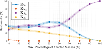
Figure 1: Percentage of times a given control policy outperforms the remaining three as a function of the maximum percentage of masses affected by uniformly distributed disturbances in the interval $[-0.5,1]$ in a system of $10$ masses. Shaded areas around the dotted lines represent the $95\%$ confidence interval around the corresponding mean values.

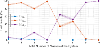
Figure 2: Percentage of times a given control policy outperforms the remaining two as a function of the number of masses constitutes the large-scale systems when totally affected by uniformly distributed disturbances in the interval $[-0.5,1]$. Shaded areas around the dotted lines represent the $95\%$ confidence interval around the corresponding mean values.

In our study, we conduct a comparative analysis to evaluate the performance of each controller when subjected to diverse and widely distributed disturbances, mimicking large-scale system scenarios. To achieve this, we perform two distinct experiments, the results of which are depicted in Figure 1 and Figure 2. In both cases, our main focus is to determine the percentage of times in which each controller yields a better (i.e., smaller) cost $J(\cdot)$ compared to the other three.

In the first experiment, we replicate the unpredictability and uncertain nature of the disturbances simulating perturbations $\bm{\delta}$ drawn from a non-centered uniform distribution $\mathcal{U}[-0.5,1]$. We then apply these disturbances to a random number of masses within the system. The percentage of affected cars is also drawn uniformly with a maximum number $N$ of affected cars. The value $N$ is incrementally increased up to the total number of the interconnected subsystems (in this case $10$). The results are presented in Figure 1. The percentage value of times each policy yields better performance is computed over $1103$ realizations of $\bm{\delta}$ and, to obtain the $95\%$ confidence interval of these measurements, we iterated this step $1102$ times, for a total of $1105$ experiments. As expected, when a small number of masses are affected, the resulting disturbance is zero for most of the agents, aligning with the $\operatorname*{\mathcal{H}_{2}}2$ hypothesis on a distribution $\mathcal{D}$ centered around $0$. However, as the number of affected masses increases, the cumulative effect of non-standard $\bm{\delta}$ on the overall system becomes more pronounced, thus favoring the performance of the controller $\mathbf{K}_{R_{QI}}$.

In the second experiment, we evaluate the performance improvement of controllers minimizing spatial regret as the sparsity structure of the large-scale system becomes more and more distributed. For this reason, we choose a QI benchmark as it strikes a favorable balance between imitating a sparse structure and a centralized one. We consider the same multi-mass spring damper system with a progressively increasing number of masses, from $3$ to $10$. For each new configuration, we synthesise again all the controllers ($\mathbf{K}_{\operatorname*{\mathcal{H}_{2}}2}$, $\mathbf{K}_{\operatorname*{\mathcal{H}_{\infty}}}$, $\mathbf{K}_{R_{QI}}$). Then, we simulate the effects of perturbations $\bm{\delta}$ drawn from a non-centered uniform distribution $\mathcal{U}[-0.5,1]$ applied to all the masses. The results are shown in Figure 2. The amount of performed experiments is the same as in the previous study case. It is evident that for small systems affected by noise, $\mathbf{K}_{\operatorname*{\mathcal{H}_{\infty}}}$ outperforms the other control policies. However, as the size of the system increases, and consequently its sparsity $\mathbf{K}_{R_{QI}}$ exhibits superior performance, highlighting its capacity to leverage information from the ideal oracle.

V Conclusions

In this work, we aimed to imp and synthesize distributed controllers for large-scale linear dynamical systems, affected by localized and highly heterogeneous disturbances. To do so, we first introduced the novel metric $\operatorname{SpRegret}$. Then we demonstrated its well-posedness. Furthermore, we have formulated the $\operatorname{SpRegret}$ minimization in a convex way. Through comparisons with classic $\operatorname*{\mathcal{H}_{2}}2$ and $\operatorname*{\mathcal{H}_{\infty}}$ policies, our results showcased the superior performance of $\operatorname{SpRegret}$ controllers in handling disturbances that may target large-scale distributed systems. However, characterizing the class of disturbances for which $\operatorname{SpRegret}$ controllers outperform classic controllers remains an open challenge.

Future research will explore novel methods for designing constrained benchmarks that ensure positive regret and improved performance over $\operatorname*{\mathcal{H}_{2}}2$ and $\operatorname*{\mathcal{H}_{\infty}}$ for user-defined disturbance classes. Additional future directions include investigating how to automatically select the sparsity structure of the oracle tailored to the problem to obtain better performance and extend our results to the infinite-horizon case.

-A Example of $\mathbf{\hat{K}}$ not Guaranteeing Well-Posedness

Consider the following scalar system

$$x_{t+1}=0.2x_{t}+0.5u_{t}+w_{t}\,.$$

Choose $T=3$, $\mathbf{C}=I$ and the two controllers $\mathbf{K}$ and $\mathbf{\hat{K}}$ as

$$\scalebox{0.9}{\mbox{$\displaystyle\mathbf{K}=\begin{bmatrix}0.89&0&0\\ 2.66&-2.51&0\\ 1&-0.11&-0.7\\ \end{bmatrix},\>\>\mathbf{\hat{K}}=\begin{bmatrix}1.43&0&0\\ 3.19&-2.77&0\\ 2.01&-2.14&-1.24\\ \end{bmatrix}$}}.$$

Compute $\mathbf{\Phi}$, $\mathbf{\hat{\Phi}}$ by the definition (7). Then the error $e(\bm{\delta},\mathbf{K},\mathbf{\hat{K}})=J(\bm{\delta},\mathbf{K})-J(\bm{\delta},\mathbf{\hat{K}})$ can be rewritten in $\mathbf{\Phi}$ using (9) as

$$e(\bm{\delta},\mathbf{\Phi},\mathbf{\hat{\Phi}})=\bm{\delta}^{\top}\underbrace{\Big{(}\mathbf{\Phi}^{\top}\mathbf{C}\mathbf{\Phi}-\mathbf{\hat{\Phi}}^{\top}\mathbf{C}\mathbf{\hat{\Phi}}\Big{)}}_{\Pi}\bm{\delta}.$$

We can verify that $\Pi\preceq 0$, i.e., $e(\bm{\delta},\mathbf{\Phi},\mathbf{\hat{\Phi}})\leq 0$ for any $\bm{\delta}$. Thus, in this case the controller $\mathbf{K}$ should not imitate the oracle $\mathbf{\hat{K}}$, meaning that $\mathbf{\hat{K}}$ should not be used in (5).

-B Example that Using SI to Design Both $\mathbf{K}$, $\mathbf{\hat{K}}$ Does Not Guarantee Well-Posedness

Let $\mathbf{\Delta}=\operatorname{Struct}(\mathbf{G})=I$ and

$$\operatorname{Struct}(\mathcal{S})=\begin{bmatrix}1&0&0\\ 1&1&0\\ 0&0&1\end{bmatrix},\>\>\operatorname{Struct}(\hat{\mathcal{S}})=\begin{bmatrix}1&0&0\\ 1&1&0\\ 0&1&1\end{bmatrix}.$$

It is easy to verify that $\hat{\mathcal{S}}$ is not QI with respect to $\mathbf{G}$. Then, the matrices $V_{x}$ and $\hat{V}_{x}$ obtained using Algorithm 1 are

$$V_{x}=\begin{bmatrix}1&0&0\\ 1&1&0\\ 0&0&1\end{bmatrix}\,,\>\>\hat{V}_{x}=\begin{bmatrix}1&0&0\\ 0&1&0\\ 0&1&1\end{bmatrix}.$$

It is clear that $V_{x}\nleq\hat{V}_{x}$, and thus, $\mathbf{\Theta}\nsubseteq\mathbf{\hat{\Theta}}$. Consequently, the $\operatorname{SpRegret}$ is not guaranteed to be well-posed in this case.

-C Implementation Details

The model of the system is described as follows. The state $x^{i}(\tau)$ of each mass $i$ is $x^{i}(\tau)=\begin{bmatrix}{p}^{i}(\tau)\\ {v}^{i}(\tau)\end{bmatrix}$, where $p^{i}(\tau)$ and $v^{i}(\tau)$ represent the position and velocity of the mass $i\in\{1,\dots,10\}$ at time $\tau$. Each mass has a value of $m=$1\text{\,}\mathrm{kg}$$ and is interconnected with its adjacent masses via dampers with $c=$0.5\text{\,}\mathrm{kg}\text{\,}{\mathrm{s}}^{-1}$$ and springs with $k=$0.5\text{\,}\mathrm{k}\mathrm{g}\mathrm{/}\mathrm{s}^{2}$$. The dynamics of each mass $i$ is influenced by the states of its left and right neighbors $x^{i-1}(\tau)$ and $x^{i+1}(\tau)$. The end masses $x^{1}(\tau)$ and $x^{10}(\tau)$ do not present any left and right neighbors, respectively.

The state evolution is described by

We discretize this system with a sampling time of $T_{s}=$0.5\text{\,}\mathrm{s}$$, and set $\mathbf{C}=I$ to minimize input action and bring the states to zero. The sparsity matrix $\mathbf{S}$ is defined as

$$\mathbf{S}=\textnormal{Tril}(T)\otimes\bNiceArray{>{}llllllllll}[margin=1mm]\Block[borders={bottom,top,right,left,tikz={dashed,red}}]{1-3}{}1&11{}{}{}{}{}\Block[borders={bottom,top,right,left,tikz={dashed,red}}]{5-2}{}11\\ {}{}\Block[borders={bottom,top,right,left,tikz={dashed,red}}]{1-3}{}111{}{}{}11\\ {}{}{}{}{}\ddots{}{}\vdots\vdots\\ {}{}{}{}{}{}\Block[borders={bottom,top,right,left,tikz={dashed,red}}]{1-3}{}1111\\ {}{}{}{}{}{}{}{}\Block[borders={bottom,top,right,left,tikz={dashed,red}}]{1-2}{}11\\ .$$

This means that the controller of each mass has access to the mass of its own agent plus the position of its right neighbor. Additionally, every controller has knowledge of the state $x^{10}$ of the last agent.

Reducing the Computation Load. Problem (23) is a semidefinite optimization problem that exhibits a quadratic growth in the number of variables with respect to $T$: this can pose scalability challenges even for relatively short time windows. To mitigate this issue, inspired by infinite-horizon methods and following [22], we employ an approximation technique that favors scalability. Specifically, we introduce constraints on $\mathbf{\Phi}_{u}$ as described in (8)). We impose a lower-block Toeplitz diagonal matrix structure, which we denote as $\bar{\mathbf{\Phi}}_{u}$.

Consequently $\bar{\mathbf{\Phi}}_{x}$ is obtained by $\bar{\mathbf{\Phi}}_{x}=(I+\mathbf{Z}\mathbf{A})^{-1}(I+\mathbf{Z}\mathbf{B}\bar{\mathbf{\Phi}}_{u})$ to guarantee (8). This approach significantly reduces the total number of variables in (23) to $(mnT+1)$, which now is linear in $T$.

References

- [1] D. K. Molzahn, F. Dörfler, H. Sandberg, S. H. Low, S. Chakrabarti, R. Baldick, and J. Lavaei, “A survey of distributed optimization and control algorithms for electric power systems,” IEEE Transactions on Smart Grid, vol. 8, no. 6, pp. 2941–2962, 2017.
- [2] Y. Zheng, S. E. Li, K. Li, F. Borrelli, and J. K. Hedrick, “Distributed model predictive control for heterogeneous vehicle platoons under unidirectional topologies,” IEEE Transactions on Control Systems Technology, vol. 25, no. 3, pp. 899–910, 2016.
- [3] H. S. Witsenhausen, “A counterexample in stochastic optimum control,” SIAM Journal on Control, vol. 6, no. 1, pp. 131–147, 1968.
- [4] M. Rotkowitz and S. Lall, “A characterization of convex problems in decentralized control,” IEEE transactions on Automatic Control, vol. 50, no. 12, pp. 1984–1996, 2005.
- [5] L. Lessard and S. Lall, “Quadratic invariance is necessary and sufficient for convexity,” in Proceedings of the 2011 American Control Conference, pp. 5360–5362, IEEE, 2011.
- [6] L. Furieri and M. Kamgarpour, “Unified approach to convex robust distributed control given arbitrary information structures,” IEEE Transactions on Automatic Control, vol. 64, no. 12, pp. 5199–5206, 2019.
- [7] Y.-S. Wang, N. Matni, and J. C. Doyle, “A system-level approach to controller synthesis,” IEEE Transactions on Automatic Control, vol. 64, no. 10, pp. 4079–4093, 2019.
- [8] L. Furieri, Y. Zheng, A. Papachristodoulou, and M. Kamgarpour, “Sparsity invariance for convex design of distributed controllers,” IEEE Transactions on Control of Network Systems, vol. 7, no. 4, pp. 1836–1847, 2020.
- [9] E. Jensen and B. Bamieh, “An explicit parametrization of closed loops for spatially distributed controllers with sparsity constraints,” IEEE Transactions on Automatic Control, vol. 67, no. 8, pp. 3790–3805, 2021.
- [10] S. Fattahi, G. Fazelnia, J. Lavaei, and M. Arcak, “Transformation of optimal centralized controllers into near-globally optimal static distributed controllers,” IEEE Transactions on Automatic Control, vol. 64, no. 1, pp. 66–80, 2018.
- [11] B. Hassibi, A. H. Sayed, and T. Kailath, Indefinite-Quadratic estimation and control: a unified approach to and theories. SIAM, 1999.
- [12] O. Sabag, G. Goel, S. Lale, and B. Hassibi, “Regret-optimal controller for the full-information problem,” in 2021 American Control Conference (ACC), pp. 4777–4782, IEEE, 2021.
- [13] G. Goel and B. Hassibi, “Regret-optimal estimation and control,” IEEE Transactions on Automatic Control, vol. 68, no. 5, pp. 3041–3053, 2023.
- [14] A. Martin, L. Furieri, F. Dörfler, J. Lygeros, and G. Ferrari-Trecate, “Safe control with minimal regret,” in Learning for Dynamics and Control Conference, pp. 726–738, PMLR, 2022.
- [15] A. Didier, J. Sieber, and M. N. Zeilinger, “A system level approach to regret optimal control,” IEEE Control Systems Letters, vol. 6, pp. 2792–2797, 2022.
- [16] A. Martin, L. Furieri, F. Dörfler, J. Lygeros, and G. Ferrari-Trecate, “On the guarantees of minimizing regret in receding horizon,” arXiv preprint arXiv:2306.14561, 2023.
- [17] A. Martin, L. Furieri, F. Dörfler, J. Lygeros, and G. Ferrari-Trecate, “Follow the clairvoyant: an imitation learning approach to optimal control,” arXiv preprint arXiv:2211.07389, 2022.
- [18] U. Ghai, U. Madhushani, N. Leonard, and E. Hazan, “A regret minimization approach to multi-agent control,” in International Conference on Machine Learning, pp. 7422–7434, PMLR, 2022.
- [19] J. Anderson, J. C. Doyle, S. H. Low, and N. Matni, “System level synthesis,” Annual Reviews in Control, vol. 47, pp. 364–393, 2019.
- [20] M. C. Rotkowitz and N. C. Martins, “On the nearest quadratically invariant information constraint,” IEEE Transactions on Automatic Control, vol. 57, no. 5, pp. 1314–1319, 2011.
- [21] S. Boyd, L. El Ghaoui, E. Feron, and V. Balakrishnan, Linear matrix inequalities in system and control theory. SIAM, 1994.
- [22] J. Zhang and T. Ohtsuka, “Stochastic model predictive control using simplified affine disturbance feedback for chance-constrained systems,” IEEE Control Systems Letters, vol. 5, no. 5, pp. 1633–1638, 2021.