Hardy-type paradoxes for an arbitrary symmetric bipartite Bell scenario

Abstract

As with a Bell inequality, Hardy’s paradox manifests a contradiction between the prediction given by quantum theory and local-hidden variable theories. In this work, we give two generalizations of Hardy’s arguments for manifesting such a paradox to an arbitrary, but symmetric Bell scenario involving two observers. Our constructions recover that of Meng et al. [Phys. Rev. A. 98, 062103 (2018)] and that first discussed by Cabello [Phys. Rev. A 65, 032108 (2002)] as special cases. Among the two constructions, one can be naturally interpreted as a demonstration of the failure of the transitivity of implications (FTI). Moreover, a special case of which is equivalent to a ladder-proof-type argument for Hardy’s paradox. Through a suitably generalized notion of success probability called degree of success, we provide evidence showing that the FTI-based formulation exhibits a higher degree of success compared with all other existing proposals. Moreover, this advantage seems to persist even if we allow imperfections in realizing the zero-probability constraints in such paradoxes. Explicit quantum strategies realizing several of these proofs of nonlocality without inequalities are provided.

I Introduction

In the thought-provoking paper by Einstein, Podolksy, and Rosen [1], the strong correlations between measurement outcomes have led them to suspect that quantum theory could be somehow completed (with additional variables). This was eventually shown to be untenable by Bell [2], who proved that no local-hidden-variable (LHV) models can reproduce all quantum-mechanical predictions. In particular, he demonstrated how, with the help of so-called Bell inequalities, one can experimentally falsify the predictions of LHV models. Nowadays, we know that Bell nonlocality not only opens the door to answer fundamental questions in physics but also serves as an important resource for device-independent quantum information [3, 4].

Interestingly, Bell inequalities are not the only way to manifest Bell nonlocality [3]. Indeed, Greenberger, Horne, and Zeilinger (GHZ) [5] showed in their seminal work that a logical contradiction can be demonstrated between the quantum mechanical prediction on a four-qubit GHZ state and that of any deterministic LHV model (DLHVM). Soon after, such a contradiction was also provided for a three-qubit GHZ state [6] and a two-qubit singlet state [7]. This last construction, in particular, was adapted to give the well-known Peres-Mermin game [8] for showing quantum pseudo-telepathy.

A common feature of these logical proofs is that they rely strongly on the perfect correlation of maximally entangled states. In contrast, Hardy [9] provided a different type of logical proof of “nonlocality without inequality” for a partially entangled two-qubit state. In Hardy’s proof, a contradiction comes about only when a certain event is observed, see Fig. 1. The probability at which this event occurs is thus commonly called the success probability, as it facilitates (initiates) the chain of logical reasoning in Hardy’s arguments.

Hardy’s original proof was soon generalized to cater for certain bipartite quantum states of arbitrary local Hilbert space dimension [10], an arbitrary number of qubit systems [11] (see also [12, 13]), an arbitrary partially entangled two-qubit state [14], and later to an experimental scenario involving an arbitrary number of binary-outcome measurement settings [15]. In the meantime, Stapp [16] showed that Hardy’s argument (which leads to the so-called Hardy paradox) can also be interpreted as the failure of the transitivity implications (FTI), thereby demonstrating Bell nonlocality (see also [17]).

(a) Hardy’s argument

(b) Stapp’s argument

Figure 1: Schematic representation of (a) Hardy’s argument and (b) Stapp’s reformulation [16] for demonstrating the inadequacy of DLHVMs in reproducing quantum predictions. Here, $A_{x}$ and $B_{y}$ represent, respectively, the outcome ($0$ or $1$) observed by Alice and Bob when she performs the $x$-the measurement and he performs the $y$-th measurement. In a DLHVM, the implications (black arrows) and the forbidden event (red) imply that the event $A_{1}=B_{1}=1$ is also forbidden, yet quantum theory defies this implication.

Several years later, relaxations of Hardy’s original formulation were also proposed. For example, motivated by Kar’s observation [18] that no mixed two-qubit entangled states exhibit Hardy’s paradox, Liang and Li [19, 20] generalized Hardy’s argument by relaxing one of the equality constraints to an inequality constraint (see also[21]). Indeed, their construction allowed them to demonstrate a Hardy-type logical contradiction for certain mixed two-qubit states via a generalized notion of success probability, called degree of success in [22]. Subsequently, Kunkri et al. [23] showed that this generalization could give a higher degree of success compared to the original formulation in [14]. A brief discussion of a further generalization from Cabello and that of Liang-Li to a scenario with an arbitrary number of measurement settings was subsequently given in [24].

Indeed, a noticeably higher success probability (or degree of success) can be obtained if we are willing to consider a Bell scenario with more measurement settings [15, 24], outcomes [25], or both [26]. As with [26], in this work, we propose two generalizations of Hardy’s arguments applicable to an arbitrary (symmetric) bipartite Bell scenario, which recovers, respectively, that of [26] and that discussed by [20, 23, 24] as a special case. We provide evidence showing that the one that can be interpreted as a demonstration of FTI leads to a degree of success higher than all those offered by other existing proposals, even in the presence of noise.

II Hardy’s paradox and its generalization in the simplest Bell scenario

II.1 Hardy’s original formulation

Consider the simplest Clauser-Horne-Shimony-Holt (CHSH) Bell scenario, i.e., one in which two observers each perform two binary-outcome measurements. Let $x$ and $y$ ($a$ and $b$) represent, respectively, the setting/ input (outcome/ output) of Alice and Bob side, and $A_{x}$ ($B_{y}$) $=0,1$ denotes the outcome of Alice (Bob) when given input $x$ ($y$) $=0,1$. The probability distribution $\{P(a,b|x,y)=P(A_{x},B_{y})\}$ admissible in LHV models can be described by convex mixtures of local deterministic strategies $\{A_{x}=f_{A}(x,\lambda),B_{y}=f_{B}(y,\lambda)\}$, where $f_{A}$ ($f_{B}$) is a deterministic function of the input $x$ ($y$) and LHV $\lambda$. The Hardy paradox of [14] is encapsulated by:

$$\begin{split}&P(0,0|0,0)=0,\quad P(1,1|0,1)=0,\\ &P(1,1|1,0)=0,\quad P(1,1|1,1)=q>0.\end{split}$$ (1)

For DLHVMs, the equality constraints of Eq. 1 imply $P(1,1|1,1)=0$, which contradicts the inequality constraint of Eq. 1. In other words, together with the equality constraints, the occurrence of the event $x=y=a=b=1$ contradicts the prediction of any DLHVM. Consequently, the quantity $q\equiv P(1,1|1,1)$ is also known as the success probability. In quantum theory, it is known [27] that the maximal attainable success probability is $\frac{5\sqrt{5}-11}{2}\approx 9.02\%$. Finally, note that a general LHV model can always be seen mathematically as a convex mixture of DLHVM. Thus, the observation of Eq. 1 also rules out a general LHV model.

II.2 Generalization due to Cabello-Liang-Li

Cabello’s [21] relaxation of Hardy’s argument, originally proposed for a tripartite scenario and subsequently applied in the bipartite scenario by Liang and Li [20], takes the form:

$$\begin{split}P(0,0|0,0)=p,\quad P(1,1|0,1)=0,\\ P(1,1|1,0)=0,\quad P(1,1|1,1)=q.\end{split}$$ (2)

Hereafter, we refer to this as the Cabello-Liang-Li (CLL) argument. Compared with Eq. 1, we see that in this argument, $P(0,0|0,0)$ is allowed to take nonzero value. From Fig. 1(a), we see that for any DLHVM, if the event $x=y=a=b=1$ occurs, so must the event $x=y=a=b=0$. However, there exist other local deterministic strategies (e.g., one where $a=b=0$ regardless of $x$ and $y$) where the latter event occurs while the former does not. Thus, for the prediction of a general LHV model, we must have $p\equiv P(0,0|0,0)\geq q\equiv P(1,1|1,1)$. In other words, one may take the positive value of the quantity

$$q-p=P(1,1|1,1)-P(0,0|0,0)$$ (3)

as a witness for successfully demonstrating a logical contradiction based on such an argument. In [23], the authors refer to $q-p$ as the success probability of such an argument. However, since $q-p$ is the difference between two conditional probabilities, we shall follow [22] and refer to $q-p$ instead as the degree of success. In [23], the authors showed that this degree of success can reach $\approx 10.79\%$.

II.3 Our generalization based on FTI

Using Stapp’s reformulation [16] of Eq. 1 as an FTI, we now provide a different relaxation of Hardy’s paradox via:

$$\begin{split}P(0,0|0,0)=0,\quad P(1,1|0,1)=r,\\ P(1,1|1,0)=0,\quad P(1,1|1,1)=q,\end{split}$$ (4)

From Fig. 1(b), we see that for any DLHVMs, if the event $x=y=a=b=1$ occurs, so must the event for $x=0$ and $y=a=b=1$. However, there are local deterministic strategies where the converse does not hold. Thus, for a general LHV model (obtained by averaging the deterministic ones), we must have $r\equiv P(1,1|0,1)\geq q\equiv P(1,1|1,1)$. Hence, in analogy with the CLL argument, we refer to

$$q-r=P(1,1|1,1)-P(1,1|0,1)$$ (5)

as the degree of success of such an argument. In [28], it was shown that in quantum theory, the largest value of $q-r$ is $\frac{1}{8}=12.5\%$, attainable by performing projective measurements on a two-qubit pure state and higher than that achievable with Eq. 2.

II.3.1 Maximal degree of success for $2$-qubit pure states

In fact, the general two-qubit pure state and observables satisfying the zero-probability constraints of Eq. 4 are [28]:

$$\ket{\psi}=\sin\theta\left(\cos{\alpha}\ket{0}-\sin\alpha\ket{1}\right)\!\ket{1}+\cos\theta\ket{1}\!\ket{0},$$ (6a)

$$\begin{split}A_{0}=\sigma_{z},\quad A_{1}=\cos{2\alpha}\,\sigma_{z}-\sin{2\alpha}\,\sigma_{x},\\ B_{0}=\sigma_{z},\quad B_{1}=\cos{2\beta}\,\sigma_{z}-\sin{2\beta}\,\sigma_{x},\end{split}$$ (6b)

where $\theta,\alpha,\beta\in[0,\pi]$. From here, the corresponding degree of success of Eqs. 5 and 6, as a function of the parameters $\theta$, $\alpha$, and $\beta$ can be shown to be:

$$\begin{split}P_{\text{succ}}(\theta,\alpha,\beta)=&\frac{1}{2}\sin{\alpha}\left[\left(\cos{2\beta}\cos{2\theta}-1\right)\sin{\alpha}\right.\\ &\left.+\sin{2\beta}\sin{2\theta}\right]\end{split}$$ (7)

Naturally, one may wonder which entangled two-qubit pure state gives the largest value of $P_{\text{succ}}$. To this end, note that the entanglement of the two-qubit state of Eq. 6a, as measured according to the concurrence [29], is

$$C(\ket{\psi})=|\sin{2\theta}\cos{\alpha}|.$$ (8)

Using variational techniques, the largest degree of success that we have found for given concurrence $C$ is

$$P^{*}_{\text{succ}}(C)=\frac{\sqrt{1-C^{2}}}{2}\left(1-\sqrt{1-C^{2}}\right),$$ (9)

for which $\theta=\beta\in\{\frac{\pi}{4},\frac{3\pi}{4}\}$. From Fig. 2, it is clear that for any given concurrence, this degree of success is always larger that from the CLL argument, which, in turn, is larger than that from Hardy’s original formulation.

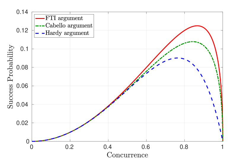
Figure 2: The maximal degree of success (which reduces to the success probability in the Hardy argument) in demonstrating a proof of nonlocality without inequality for given concurrence [29]. From top to bottom, we plot $q-r$ of Eq. 4 for our FTI argument (red, solid), $q-p$ of Eq. 2 for CLL’s argument (green, dashed, see [23]), and $q$ of Eq. (1) for Hardy’s argument (blue, dashed-dotted, see [14]). Note that the entangled state that gives the largest degree of success differs from one formulation to the other.

II.3.2 FTI argument with noise

Evidently, imperfections in any realistic experimental scenario make it essentially impossible to realize the zero-probability equality constraints in all these different formulations. To understand the impact of these imperfections, we now relax Eq. 4 and consider

$$\begin{split}P(0,0|0,0)\leq\epsilon,\quad P(1,1|0,1)=r,\\ P(1,1|1,0)\leq\epsilon,\quad P(1,1|1,1)=q,\end{split}$$ (10)

where $\epsilon$ is the error bound. For the CLL argument, the same discussion has been made in [22]. In Fig. 3, we show the corresponding maximal degree of success, i.e., $q-r$ from Eq. 10, when the noise $\epsilon\in(0,0.5)$. Our results clearly show that for any amount of noise in this range, the FTI argument gives a higher maximal degree of success compared to the CLL one.

Note that for our relaxed FTI argument of Eq. 10, upper bounds on the maximum degree of success (based on level-3 of the semidefinite programming (SDP) hierarchy introduced in [30]) coincide with the lower bounds (based on two-qubit pure state with rank-1 projective measurements) to within a numerical precision of $10^{-7}$. However, if we consider only qubit strategies, then as already noted in [22] (see their Fig. 1), there appears to be a gap between the maximal degree of success achievable with such strategies and the upper bound obtained from SDP for some values of $\epsilon$. Upon closer inspection, we find that for $0.158\lesssim\epsilon<0.5$, the SDP upper bound is attainable to within the same precision by considering a convex mixture of the qubit strategy for $\epsilon=0.158$ and $\epsilon=1$, or equivalently a ququart strategy obtained from their direct sum.

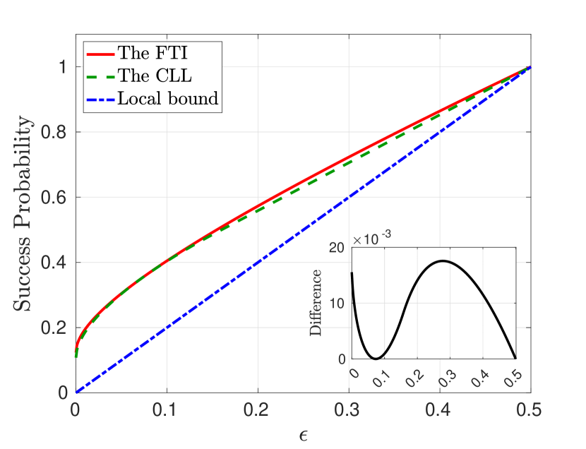
Figure 3: Degree of success as a function of the deviation $\epsilon$ from the zero-probability constraints. The top curve (red, solid) shows a lower bound on the degree of success for our FTI argument (obtained by optimizing over two-qubit states and projective measurements); the middle curve (green, dashed) shows an upper bound on the degree of success for CLL’s argument (see also [22]) obtained using level-3 of the semidefinite programming (SDP) hierarchy described in Ref. [30]. The inset is to highlight the difference between the two degrees of success (provided, respectively, by our FTI argument and the CLL argument), which is always positive within a numerical precision of $10^{-7}$. Note that two probabilities coincide when $\epsilon\approx 0.0730$.

III Generalization of Hardy’s proof beyond the simplest Bell scenario

Figure 4: Summary of the relationships between the various Hardy-type paradoxes discussed in this work. Our new constructions are printed in boldface.

Having understood how Hardy and Hardy-type paradoxes work in the simplest Bell scenario, the time is now ripe to discuss their generalization to more complex Bell scenarios. In this section, we propose, respectively, a generalization of both the Hardy-type paradox of CLL, Eq. 2, and that based on FTI, Eq. 4, to an arbitrary bipartite $k$-input $d$-output Bell scenario, i.e., one in which both party has a choice over $k$ alternative $d$-outcome measurements.

III.1 Generalization of CLL Hardy-type paradox

Specifically, for the CLL Hardy-type paradox, the following conditions on the joint conditional probabilities:

$$\left\{\begin{aligned} &P(A_{k-1}<B_{k-1})=q,\leavevmode\nobreak\ \text{if}\leavevmode\nobreak\ k\in\text{odd},\\ &P(A_{k-1}>B_{k-1})=q,\leavevmode\nobreak\ \text{if}\leavevmode\nobreak\ k\in\text{even},\end{aligned}\right.$$ (11a)

$$P(A_{i}>B_{i-1})=0,\leavevmode\nobreak\ \forall\leavevmode\nobreak\ i\in\text{odd}\cap\{1,\cdots,k-1\},$$ (11b)

$$P(A_{i}<B_{i-1})=0,\leavevmode\nobreak\ \forall\leavevmode\nobreak\ i\in\text{even}\cap\{1,\cdots,k-1\},$$ (11c)

$$P(A_{i-1}>B_{i})=0,\leavevmode\nobreak\ \forall\leavevmode\nobreak\ i\in\text{odd}\cap\{1,\cdots,k-1\},$$ (11d)

$$P(A_{i-1}<B_{i})=0,\leavevmode\nobreak\ \forall\leavevmode\nobreak\ i\in\text{even}\cap\{1,\cdots,k-1\},$$ (11e)

$$P(A_{0}<B_{0})=p,$$ (11f)

together with $q>p$ define our generalization of this paradox, where the outcomes $A_{x},B_{y}$ may take $d$ possible values, say, from $\{0,1,\cdots,d-1\}$. For the special case of $p=0$, one obtains a generalization of the original Hardy paradox to an arbitrary bipartite $k$-input $d$-output Bell scenario. If we further set $d=2$, then the construction reduces to one equivalent (under relabeling of inputs and outputs) to the ladder proof of nonlocality [15]. If, instead, we take $d=2$ in Eq. 11 without setting $p=0$, one obtains the argument briefly discussed in [24]. All these relations are summarized in Fig. 4.

Figure 5: Logical structure of the generalized CLL arguments in the $k$-input $d$-output Bell scenario. The generalization of Hardy’s original argument to these cases is recovered by setting $p=0$.

To see that the constraints of Eq. 11 with $q-p>0$ indeed constitute a proof of nonlocality without inequality, we begin by restricting our attention to a DLHVM where the measurement outcomes take definite values, denoted by $\{A_{i}=s^{A}_{i}\}$ and $\{B_{i}=s^{B}_{i}\}$, where $i\in\{0,1,\dots,k-1\}$. We depict the logical structure behind this argument schematically in Fig. 5. Let us now consider the case of even and odd $k$ separately, starting with odd $k$. Then, in order for a DLHVM to reproduce LABEL:Extend_Hardy_a, i.e., $P(A_{k-1}<B_{k-1})=q>0$, the model must produce events $\{A_{i}=s^{A}_{i}\}$ and $\{B_{i}=s^{B}_{i}\}$ such that $s^{A}_{k-1}<s^{B}_{k-1}$. Similarly, the other constraints of Eq. 11 imply constraints on the relationship between $\{s^{A}_{i}\}$ and $\{s^{B}_{i}\}$, where $i\in\{0,1,\dots,k-1\}$. For example, together with the conditions of Eq. 11c and Eq. 11e for $i=k-1$, i.e., $P(A_{k-1}<B_{k-2})=0$ and $P(A_{k-2}<B_{k-1})=0$, we get

$$s^{B}_{k-2}\leq s^{A}_{k-1}<s^{B}_{k-1}\leq s^{A}_{k-2}.$$ (12)

By considering the other zero-probability constraints one at a time for the remaining $i$, we arrive at

$$s^{A}_{0}\leq\dots\leq s^{B}_{k-2}\leq s^{A}_{k-1}<s^{B}_{k-1}\leq s^{A}_{k-2}\leq\dots\leq s^{B}_{0}.$$ (13)

This means that for any DLHVMs that give $s^{A}_{k-1}<s^{B}_{k-1}$, the constraints of Eq. 13 imply that they must also give $s^{A}_{0}<s^{B}_{0}$. However, there can be other DLHVMs where $s^{A}_{0}<s^{B}_{0}$ holds even though $s^{A}_{k-1}\not<s^{B}_{k-1}$. Thus, for a general LHV model, the conditions of Eq. 13 imply that $p\geq q$. In other words, a nonzero value of the degree of success $q-p$ witness Bell nonlocality without resorting to a Bell inequality.

Similarly, for even $k$, starting from $P(A_{k-1}>B_{k-1})=q>0$ and by considering the other zero-probability constraints lead to, for any DLHVMs,

$$s^{A}_{0}\leq\dots\leq s^{A}_{k-2}\leq s^{B}_{k-1}<s^{A}_{k-1}\leq s^{B}_{k-2}\leq\dots\leq s^{B}_{0}.$$ (14)

Again, this observation implies that $p\geq q\Leftrightarrow p-q\geq 0$ for any LHV model for all $k\geq 2$ and $d\geq 2$.

III.2 Generalization of the FTI-based Hardy-type paradox

Next, let us describe our generalization of the FTI-based Hardy-type paradox from Eq. 4, which consists of the following conditions:

$$P(A_{k-1}<B_{k-1})=q,$$ (15a)

$$P(A_{i}<B_{i-1})=0,\leavevmode\nobreak\ \forall\leavevmode\nobreak\ i\in\{1,\cdots,k-1\},$$ (15b)

$$P(B_{i-1}<A_{i-1})=0,\leavevmode\nobreak\ \forall\leavevmode\nobreak\ i\in\{1,\cdots,k-1\},$$ (15c)

$$P(A_{0}<B_{k-1})=r,$$ (15d)

and the requirement of $q>r$. The special case of $r=0$, which can be seen as a generalization of Stapp’s argument [16], has been proposed and discussed in [26]. To recover Eq. 4 from Eq. 15, one sets $k=d=2$ and apply the relabeling $A_{i}=0\leftrightarrow A_{i}=1$ for all $i\in\{0,1\}$. In Fig. 6, we depict schematically the logical structure of this paradox.

As with our explanation to Eq. 11, for any DLHVM satisfying $P(A_{k-1}<B_{k-1})=q>0$, the model must produce events $\{A_{i}=s^{A}_{i}\}$ and $\{B_{i}=s^{B}_{i}\}$ such that $s^{A}_{k-1}<s^{B}_{k-1}$. At the same time, the other inequality constraints from Eq. 15 imply $s^{B}_{k-2}\leq s^{A}_{k-1}$, $s^{A}_{k-2}\leq s^{B}_{k-2}$, etc., leading to

$$s^{A}_{0}\leq s^{B}_{0}\leq\dots\leq s^{A}_{k-2}\leq s^{B}_{k-2}\leq s^{A}_{k-1}<s^{B}_{k-1},$$ (16)

which implies $s^{A}_{0}<s^{B}_{k-1}$. This means that with the zero-probability constraints, a DLHVM equipped with a strategy giving $s^{A}_{k-1}<s^{B}_{k-1}$ must also give $s^{A}_{0}<s^{B}_{k-1}$. Again, other DLHVM may give $s^{A}_{0}<s^{B}_{k-1}$ even though $s^{A}_{k-1}\not<s^{B}_{k-1}$. Thus, from Eq. 15d, we conclude that for a general LHV model (obtained by averaging over local deterministic strategies), we must have $r\geq q\Leftrightarrow r-q\geq 0$ for all $k,d\geq 2$.

Figure 6: Logical structure of our FTI arguments in the $k$-input $d$-output Bell scenario. Generalized Stapp’s arguments as introduced in [26] are recovered by setting $r=0$.

III.3 Proof of equivalence of generalized Stapp’s proof and generalized ladder proof of nonlocality

Interestingly, the authors of [26] proved that in the $k$-input $2$-output scenario, the generalized Stapp’s argument, Eq. 15 with $r=0$, and the ladder proof of nonlocality, cf. Eq. 11 with $p=0$, are equivalent. In other words, these two sets of conditions can be obtained from each other via an appropriate relabeling of inputs and outputs. In what follows, we show that this equivalence also holds for arbitrary $k,d\geq 2$.

Theorem III.1.

For any symmetric bipartite Bell scenario, the set of conditions given in Eq. 11 with $p=0$ is equivalent to the set of conditions of Eq. 15 with $r=0$.

Proof.

Let us rewrite Alice’s and Bob’s measurement outcomes in Eq. 11, respectively, as $A^{\prime}_{x^{\prime}}$ and $B^{\prime}_{y^{\prime}}$, and let

$$\mathscr{L}_{1k-}:=\{1,2,\ldots,\lfloor\tfrac{k}{2}\rfloor-1\},\quad\mathscr{L}_{1k}:=\mathscr{L}_{1k-}\cup\{\lfloor\tfrac{k}{2}\rfloor\}$$

$$\mathscr{L}_{0k-}:=\{0\}\cup\mathscr{L}_{1k-},\quad\mathscr{L}_{0k}:=\mathscr{L}_{0k-}\cup\{\lfloor\tfrac{k}{2}\rfloor\}$$ (17)

For odd $k$, one may verify that the following relabeling

$$\begin{split}A^{\prime}_{x^{\prime}}=\left\{\begin{array}[]{ll}A_{\ell-1},&x^{\prime}=k-2\ell\leavevmode\nobreak\ \land\leavevmode\nobreak\ \ell\in\mathscr{L}_{1k}\\ A_{k-1-\ell},&x^{\prime}=k-1-2\ell\leavevmode\nobreak\ \land\leavevmode\nobreak\ \ell\in\mathscr{L}_{0k}\end{array}\right.,\\ B^{\prime}_{y^{\prime}}=\left\{\begin{array}[]{ll}B_{k-1},&y^{\prime}=k-1\\ B_{k-1-\ell},&y^{\prime}=k-2\ell\leavevmode\nobreak\ \land\leavevmode\nobreak\ \ell\in\mathscr{L}_{1k}\\ B_{\ell-1},&y^{\prime}=k-1-2\ell\leavevmode\nobreak\ \land\leavevmode\nobreak\ \ell\in\mathscr{L}_{1k}\end{array}\right.,\\ \end{split}$$ (18)

transforms the $2k$ conditions of Eq. 11 to those of Eq. 15. To see this, note that under this transformation, the condition of LABEL:Extend_Hardy_a stays as

$$P(A^{\prime}_{k-1}<B^{\prime}_{k-1})=P(A_{k-1}<B_{k-1})=q,$$ (19)

which is Eq. 15a. With the transformation, the conditions of Eq. 11b, Eq. 11d, Eq. 11c, and Eq. 11f with $p=0$, respectively, become the requirements that each of the following probabilities vanish:

$$P(A^{\prime}_{k-2\ell}>B^{\prime}_{k-2\ell-1})=P(A_{\ell-1}>B_{\ell-1}),\,\,\ell\in\mathscr{L}_{1k},$$

$$P(A^{\prime}_{k-2\ell-1}>B^{\prime}_{k-2\ell})=P(A_{k-1-\ell}>B_{k-1-\ell}),\,\,\ell\in\mathscr{L}_{1k};$$

$$P(A^{\prime}_{k-2\ell-1}<B^{\prime}_{k-2\ell-2})=P(A_{k-1-\ell}<B_{k-2-\ell}),\,\,\ell\in\mathscr{L}_{0k-};$$

$$P(A^{\prime}_{0}<B^{\prime}_{0})=P(A_{\frac{k-1}{2}}<B_{\frac{k-1}{2}-1}).$$ (20)

In addition, the conditions of Eq. 11e become

$$P(A^{\prime}_{k-2\ell-2}<B^{\prime}_{k-2\ell-1})=P(A_{\ell}<B_{\ell-1}),\,\,\ell\in\mathscr{L}_{1k-}\text{ and}$$

$$P(A^{\prime}_{k-2}<B^{\prime}_{k-1})=P(A_{0}<B_{k-1}),$$ (21)

To summarize, the requirement that the probabilities in the first two lines of Section III.3 vanish is identical to the condition of Eq. 15b, the requirement that the probabilities in the last two lines of Section III.3 and the first line of  Section III.3 vanish is identical to the condition of Eq. 15c, and the requirement that the probability in the last line of Section III.3 vanishes is identical to the condition of Eq. 15d.

Similarly, for even $k$, one can verify that the following relabeling

$$\begin{split}A^{\prime}_{x^{\prime}}=\left\{\begin{array}[]{ll}d-1-A_{\ell-1},&x^{\prime}=k-2\ell\leavevmode\nobreak\ \land\leavevmode\nobreak\ \ell\in\mathscr{L}_{1k}\\ d-1-A_{k-1-\ell},&x^{\prime}=k-1-2\ell\leavevmode\nobreak\ \land\leavevmode\nobreak\ \ell\in\mathscr{L}_{0k}\end{array}\right.,\\ B^{\prime}_{y^{\prime}}=\left\{\begin{array}[]{ll}d-1-B_{k-1},&y^{\prime}=k-1\\ d-1-B_{k-1-\ell},&y^{\prime}=k-2\ell\leavevmode\nobreak\ \land\leavevmode\nobreak\ \ell\in\mathscr{L}_{1k}\\ d-1-B_{\ell-1},&y^{\prime}=k-1-2\ell\leavevmode\nobreak\ \land\leavevmode\nobreak\ \ell\in\mathscr{L}_{1k}\end{array}\right.,\\ \end{split}$$ (22)

transforms the $2k$ conditions of Eq. 11 to those of Eq. 15. ∎

For completeness, we show in Footnote 2 bounds on the the maximal degree of success found for different Hardy-type paradoxes in several $k$-input $2$-output and $k$-input $3$-output Bell scenarios; analogous results for a larger number of outputs are shown in Table 2. One worth noticing thing is that for all these numerical results, we observe that the degree of success from our FTI arguments is always higher than that obtained from all these other proposals.

$k$		$2$	$3$	$4$	$5$	$6$
Boschi [15]	UB	$0.09020$	$0.17459$	$0.23132$	$0.27095$	$0.29999$
	LB	$0.09017^{*}$	$0.17455$	$0.23126$	$0.27088$	$0.29995$
Cereceda [24]	UB	$0.10785$	$0.18523$	$0.23801$	$0.27546$	$0.30327$
	LB	$0.10781^{*}$	$0.18519$	$0.23796$	$0.27542$	$0.30321$
FTI-based	UB	$0.12501$	$0.20713$	$0.25976$	$0.29579$	$0.32192$
	LB	$0.125^{*}$	$0.20711$	$0.25973$	$0.29576$	$0.32190$

(a) Results for binary-output Bell scenarios. From top to bottom, we list the results for Hardy paradox given by the ladder proof of nonlocality without inequality [15] (see also [26]), generalized CLL’s argument due to [24], and our FTI-based formulation [Eq. 15]. The quantum strategies corresponding to the LBs are provided in [31]. Entries marked with * are known to be tight quantum bound.

$k$		$2$	$3$	$4$	$5$
Meng [26]	UB	$0.14194$	$0.26782$	$0.34823$	$0.40196$
	LB	$0.14189$	$0.26779$	$0.34816$	$0.40184$
CLL-type	UB	$0.16794$	$0.28272$	$0.35706$	$0.40763$
	LB	$0.16791$	$0.28265$	$0.35698$	$0.40753$
FTI-based	UB	$0.19313$	$0.31230$	$0.38467$	$0.43225$
	LB	$0.19309$	$0.31226$	$0.38460$	$0.43216$

(b) Results for ternary-output Bell scenarios. From top to bottom, we list the results for generalized Hardy paradox given by Meng et al. [26], our generalized CLL formulation [Eq. 11], and our FTI-based formulation [Eq. 15]. The quantum strategies corresponding to the LBs are provided in [31].

Table 1: Comparison of the best upper bound (UB) and the best lower bound (LB) found on the degree of success for three different Hardy and Hardy-type paradoxes beyond the CHSH scenarios with $k\geq 2$ inputs. See also Fig. 4 for the relationship between all these paradoxes. The UBs were obtained by considering level-1 of the SDP hierarchy introduced in Ref. [30]. The LBs, obtained numerically, may be attained using the strategies provided in [31] (see also Appendix A).

$d$		$2$	$3$	$4$	$5$	$6$	$7$
Chen [25]	UB	$0.09020$	$0.14194$	$0.17769$	$0.20470$	$0.22623$	$0.24406$
	LB	$0.09017^{*}$	$0.14189$	$0.17657$	$0.20489$	$0.22425$	$0.13768$
CLL-type	UB	$0.10785$	$0.16794$	$0.20945$	$0.24116$	$0.26643$	$0.28726$
	LB	$0.10781^{*}$	$0.16791$	$0.20883$	$0.23987$	$0.25903$	$0.14923$
FTI-based	UB	$0.12501$	$0.19313$	$0.23844$	$0.27181$	$0.29787$	$0.31904$
	LB	$0.125^{*}$	$0.19309$	$0.23839$	$0.27175$	$0.29526$	$0.15888$

Table 2: Comparison of the best upper bound (UB) and the best lower bound (LB) found on the degree of success for the Hardy paradox due to [25], our generalized CLL formulation [Eq. 11], and our FTI-based formulation [Eq. 15] for Bell scenarios with two inputs and $d\geq 2$ outputs. See also Fig. 4 for the relationship between all these paradoxes. The UBs were obtained by considering level-1 of the SDP hierarchy introduced in Ref. [30] (see also Footnote 2). The LBs, obtained numerically, may be attained using the strategies provided in [31]. Entries marked with * are known to be tight quantum bound.

IV Discussion

Hardy and Hardy-type paradoxes are fascinating proofs of Bell nonlocality without resorting to Bell inequalities. Aside from fundamental interests (see, e.g., [32, 33, 34, 28]), they are also known to be relevant in the task of randomness amplification [35] (see, e.g., [36, 37]). In this work, we propose a Hardy-type paradox that can be naturally understood via the failure of the transitivity of implications (FTI), cf. [16, 17].

As with the Hardy-type paradoxes formulated by Cabello-Liang-Li (CLL) [21, 20], we show that a degree of success generalizing the notion of success probability—whose non-negative value witnesses Bell-nonlocality—may be introduced for the FTI-based Hardy-type paradox. In the simplest Bell scenario with two inputs and two outputs, we show that the new FTI-based formulations give the highest degree of success among all existing (i.e., Hardy, CLL, and FTI-based) formulations. Moreover, this advantage persists even when the zero-probability constraints required in all these formulations are relaxed.

Then, we provide—as with [26] for the original Hardy paradox—a generalization of the FTI-based formulation and the CLL-type formulation, to symmetric Bell scenarios involving an arbitrary number of inputs and outputs. In turn, this allows us to show that a ladder-type, cf. [15], and an FTI-based proof of nonlocality without inequality are equivalent for an arbitrary symmetric Bell scenario, thereby generalizing the result of [26] for the binary-outcome Bell scenarios.

For several simple Bell scenarios, we further observe (see Footnote 2 and Table 2) numerically that our FTI-based generalizations provide the largest value of the degree of success. A natural question left open from the current work is to determine if this trend continues to hold for an arbitrary, symmetric Bell scenario. Another closely related problem concerns the observed monotonically-increasing behavior of the degree of success when one increases either the number of inputs $k$ or the number of outputs $d$ involved within each type of logical argument — an analytic proof of this observation will be more than welcome.

On the other hand, given the close connection found [38, 28, 39] between the optimizing strategy for a Hardy paradox and its self-testing [40] property, it would also be interesting to see if the optimizing correlations found for these new generalizations are also self-testing (and non-exposed [33]). From an application perspective, one may also be interested in the potential of such correlations for device-independent applications, especially in randomness amplification [35], and proofs of Bell-nonlocality in the presence of measurement independence [32].

Appendix A Quantum Strategies

In this Appendix, we give some further information about the quantum strategies that reproduce our best lower bound (LB) on the various degrees of success shown in Footnote 2 and Table 2. The actual quantum strategies for each case are available at [31]. For convenience, we refer to the various generalizations of Hardy [14] due to Boschi et al. [15], Chen et al. [25], and Meng et al. [26] as Hardy paradoxes. Indeed, in all these three cases, the degree of success is exactly the success probability of observing such a paradox.

Next, notice that the best quantum strategies we have found for the Hardy, CLL-type, and FTI-based arguments for a $k$-input, $d$-output Bell scenario, denoted by $(k,d)$, are always attained by performing rank-1 projective measurements on a pure quantum state $\ket{\psi}$ residing in the two-qudit Hilbert space $\mathbb{C}^{d}\otimes\mathbb{C}^{d}$. However, due to numerical imprecisions, the zero-probability constraints are not always strictly enforced in all these optimal strategies found. For completeness, we list in Table 3 the largest deviation found among all the zero-probability constraints for each of these “optimal" strategies.

$(k,d)$	Hardy	CLL	FTI
$(3,2)$	$2.4065\times 10^{-14}$	$1.1241\times 10^{-14}$	$1.0108\times 10^{-15}$
$(4,2)$	$3.7173\times 10^{-14}$	$1.5651\times 10^{-15}$	$7.3663\times 10^{-16}$
$(5,2)$	$1.31\times 10^{-15}$	$3.207\times 10^{-10}$	$1.5557\times 10^{-12}$
$(6,2)$	$2.268\times 10^{-15}$	$1.6756\times 10^{-11}$	$4.0153\times 10^{-12}$
$(2,3)$	$1.4965\times 10^{-6}$	$1.3404\times 10^{-16}$	$2.9385\times 10^{-16}$
$(3,3)$	$2.4822\times 10^{-9}$	$4.9713\times 10^{-16}$	$3.8448\times 10^{-10}$
$(4,3)$	$1.6744\times 10^{-11}$	$2.075\times 10^{-14}$	$4.8237\times 10^{-14}$
$(5,3)$	$9.9977\times 10^{-14}$	$4.7704\times 10^{-14}$	$4.8075\times 10^{-12}$
$(2,4)$	$7.2538\times 10^{-7}$	$1.9799\times 10^{-16}$	$3.3075\times 10^{-16}$
$(2,5)$	$7.9181\times 10^{-5}$	$1.2006\times 10^{-6}$	$5.0784\times 10^{-8}$
$(2,6)$	$1.2162\times 10^{-4}$	$4.1223\times 10^{-4}$	$6.5519\times 10^{-5}$
$(2,7)$	$2.6871\times 10^{-3}$	$3.6214\times 10^{-3}$	$3.8616\times 10^{-4}$

Table 3: Summary of the largest zero-probability-constraint violation for each optimal strategy [31] used to give the best lower bound on the degree of success presented in Footnotes 2 and 2.

References

- Einstein et al. [1935] A. Einstein, B. Podolsky, and N. Rosen, Phys. Rev. 47, 777 (1935).
- Bell [1964] J. S. Bell, Physics 1, 195 (1964).
- Brunner et al. [2014] N. Brunner, D. Cavalcanti, S. Pironio, V. Scarani, and S. Wehner, Rev. Mod. Phys. 86, 419 (2014).
- Scarani [2012] V. Scarani, Acta Physica Slovaca 62, 347 (2012).
- Greenberger et al. [1989] D. M. Greenberger, M. A. Horne, and A. Zeilinger, “Going beyond bell’s theorem,” in Bell’s Theorem, Quantum Theory and Conceptions of the Universe, edited by M. Kafatos (Springer Netherlands, Dordrecht, 1989) pp. 69–72.
- Greenberger et al. [1990] D. M. Greenberger, M. A. Horne, A. Shimony, and A. Zeilinger, Am. J. Phys. 58, 1131 (1990).
- Peres [1990] A. Peres, Phys. Lett. A 151, 107 (1990).
- Mermin [1990] N. D. Mermin, Phys. Rev. Lett. 65, 3373 (1990).
- Hardy [1992] L. Hardy, Phys. Rev. Lett. 68, 2981 (1992).
- Clifton and Niemann [1992] R. Clifton and P. Niemann, Phys. Lett. A 166, 177 (1992).
- Pagonis and Clifton [1992] C. Pagonis and R. Clifton, Phys. Lett. A 168, 100 (1992).
- Jiang et al. [2018] S.-H. Jiang, Z.-P. Xu, H.-Y. Su, A. K. Pati, and J.-L. Chen, Phys. Rev. Lett. 120, 050403 (2018).
- Luo et al. [2018] Y.-H. Luo, H.-Y. Su, H.-L. Huang, X.-L. Wang, T. Yang, L. Li, N.-L. Liu, J.-L. Chen, C.-Y. Lu, and J.-W. Pan, Sci. Bull. 63, 1611 (2018).
- Hardy [1993] L. Hardy, Phys. Rev. Lett. 71, 1665 (1993).
- Boschi et al. [1997] D. Boschi, S. Branca, F. De Martini, and L. Hardy, Phys. Rev. Lett. 79, 2755 (1997).
- Stapp [1993] H. P. Stapp, Mind, Matter and Quantum Mechanics (Springer Verlag, 1993).
- Liang et al. [2011] Y.-C. Liang, R. W. Spekkens, and H. M. Wiseman, Phys. Rep. 506, 1 (2011).
- Kar [1997] G. Kar, Phys. Lett. A 228, 119 (1997).
- Liang and Li [2003] L.-M. Liang and C.-Z. Li, Phys. Lett. A 318, 300 (2003).
- Liang and Li [2005] L.-M. Liang and C.-Z. Li, Phys. Lett. A 335, 371 (2005).
- Cabello [2002] A. Cabello, Phys. Rev. A 65, 032108 (2002).
- Rai et al. [2021] A. Rai, M. Pivoluska, M. Plesch, S. Sasmal, M. Banik, and S. Ghosh, Phys. Rev. A 103, 062219 (2021).
- Kunkri et al. [2006] S. Kunkri, S. K. Choudhary, A. Ahanj, and P. Joag, Phys. Rev. A 73, 022346 (2006).
- Cereceda [2017] J. L. Cereceda, Quantum Studies: Mathematics and Foundations 4, 205 (2017).
- Chen et al. [2013] J.-L. Chen, A. Cabello, Z.-P. Xu, H.-Y. Su, C. Wu, and L. C. Kwek, Phys. Rev. A 88, 062116 (2013).
- Meng et al. [2018] H.-X. Meng, J. Zhou, Z.-P. Xu, H.-Y. Su, T. Gao, F.-L. Yan, and J.-L. Chen, Phys. Rev. A 98, 062103 (2018).
- Rabelo et al. [2012] R. Rabelo, L. Y. Zhi, and V. Scarani, Phys. Rev. Lett. 109, 180401 (2012).
- Chen et al. [2023] K.-S. Chen, G. N. M. Tabia, C. Jebarathinam, S. Mal, J.-Y. Wu, and Y.-C. Liang, Quantum 7, 1054 (2023).
- Wootters [1998] W. K. Wootters, Phys. Rev. Lett. 80, 2245 (1998).
- Moroder et al. [2013] T. Moroder, J.-D. Bancal, Y.-C. Liang, M. Hofmann, and O. Gühne, Phys. Rev. Lett. 111, 030501 (2013).
- [31] Download ancillary files at arXiv for the explicit quantum strategies leading to these success probabilities.
- Pütz et al. [2014] G. Pütz, D. Rosset, T. J. Barnea, Y.-C. Liang, and N. Gisin, Phys. Rev. Lett. 113, 190402 (2014).
- Goh et al. [2018] K. T. Goh, J. Kaniewski, E. Wolfe, T. Vértesi, X. Wu, Y. Cai, Y.-C. Liang, and V. Scarani, Phys. Rev. A 97, 022104 (2018).
- Rai et al. [2019] A. Rai, C. Duarte, S. Brito, and R. Chaves, Phys. Rev. A 99, 032106 (2019).
- Colbeck and Renner [2012] R. Colbeck and R. Renner, Nat. Phys. 8, 450 (2012).
- Ramanathan et al. [2018] R. Ramanathan, M. Horodecki, H. Anwer, S. Pironio, K. Horodecki, M. Grünfeld, S. Muhammad, M. Bourennane, and P. Horodecki, arXiv:1810.11648 (2018).
- Zhao et al. [2023] S. Zhao, R. Ramanathan, Y. Liu, and P. Horodecki, Quantum 7, 1114 (2023).
- Rai et al. [2022] A. Rai, M. Pivoluska, S. Sasmal, M. Banik, S. Ghosh, and M. Plesch, Phys. Rev. A 105, 052227 (2022).
- Liu et al. [2023] Y. Liu, H. Y. Chung, and R. Ramanathan, “Investigations of the boundary of quantum correlations and device-independent applications,” arXiv:2309.06304 (2023).
- Šupić and Bowles [2020] I. Šupić and J. Bowles, Quantum 4, 337 (2020).