Bayesian Quantile Regression with Subset Selection: A Posterior Summarization Perspective

Abstract

Quantile regression is a powerful tool for inferring how covariates affect specific percentiles of the response distribution. Existing methods either estimate conditional quantiles separately for each quantile of interest or estimate the entire conditional distribution using semi- or non-parametric models. The former often produce inadequate models for real data and do not share information across quantiles, while the latter are characterized by complex and constrained models that can be difficult to interpret and computationally inefficient. Further, neither approach is well-suited for quantile-specific subset selection. Instead, we pose the fundamental problems of linear quantile estimation, uncertainty quantification, and subset selection from a Bayesian decision analysis perspective. For any Bayesian regression model, we derive optimal and interpretable linear estimates and uncertainty quantification for each model-based conditional quantile. Our approach introduces a quantile-focused squared error loss, which enables efficient, closed-form computing and maintains a close relationship with Wasserstein-based density estimation. In an extensive simulation study, our methods demonstrate substantial gains in quantile estimation accuracy, variable selection, and inference over frequentist and Bayesian competitors. We apply these tools to identify the quantile-specific impacts of social and environmental stressors on educational outcomes for a large cohort of children in North Carolina.

,

1 Introduction

Quantile regression estimates the functional relationship between covariates and specific percentiles of a response variable. We focus on linear quantile regression, which assumes that the $\tau$th conditional quantile for a random variable $Y$ changes linearly as a function of $p$-dimensional predictors $\boldsymbol{x}$:

$$Q_{\tau}\{Y\mid\boldsymbol{x},\boldsymbol{\beta}(\tau)\}=\boldsymbol{x}^{\intercal}\boldsymbol{\beta}(\tau).$$ (1)

Estimated across $\tau$, the coefficients $\boldsymbol{\beta}(\tau)$ summarize how the covariates affect not only the location, but also the shape of the response distribution $Y\mid\boldsymbol{x}$. This is useful when interest lies in providing a more robust and comprehensive view of the relationship between covariates and the response variable. Consequently, quantile regression methods have been been applied in diverse settings, including medicine (Kottas and Gelfand, 2001), finance (Bassett and Chen, 2002), and environmental studies (Pandey and Nguyen, 1999), among many others.

The unique insight from linear quantile regression comes from identifying predictors with heterogeneous effects $\beta_{j}(\tau)\neq\beta_{j}(\tau^{\prime})$ for some $\tau\neq\tau^{\prime}$. This capability is essential when the covariates affect higher order moments or tails of $Y\mid\boldsymbol{x}$. For instance, in childhood educational outcome studies (Section 5), it is essential to determine whether socioeconomic variables, environmental exposures, and other key factors differentially impact low, medium, or high-achieving students, which can provide far-reaching implications for policy interventions.

Broadly, there are several important components and considerations in quantile regression. First, quantile-specific linear coefficient estimates are obtained to detect potentially heterogeneous covariate effects, including both magnitude and direction. Second, quantile-specific uncertainty quantification provides important context for these coefficients and facilitates comparisons across both quantiles and variables. Third, when $p$ is moderate or large, quantile-specific subset selection provides more interpretable and parsimonious summaries and identifies the most impactful covariates across the distribution $Y\mid\boldsymbol{x}$. Each of these targets must simultaneously respect the fundamental smoothness across quantiles: estimates, uncertainties, and selections should be similar for adjacent quantiles. Finally, the algorithms that deliver these results must be scalable in both the number of observations $n$ and the number of covariates $p$.

We proceed to review existing Bayesian and frequentist methods for quantile regression, both to showcase the successes in this area and to highlight the need for methodological advances. We then introduce our approach and explain how it addresses each of the challenges above.

1.1 Separate Quantile Regressions

Separate quantile regression techniques estimate independent models for any set of quantiles, providing targeted estimation for each $\tau$. Given paired data $\{(\boldsymbol{x}_{i},y_{i})\}_{i=1}^{n}$, Koenker and Bassett Jr (1978) introduced this approach from a frequentist perspective, obtaining quantile-specific coefficient estimates by minimizing the check loss

$$\hat{\boldsymbol{\beta}}(\tau)=\mbox{arg min}_{\boldsymbol{\beta}}\sum_{i=1}^{n}\rho_{\tau}\{y_{i},\boldsymbol{x}_{i}^{\intercal}\boldsymbol{\beta}(\tau)\}$$ (2)

where $\rho_{\tau}(a,b)=\{a-b(\tau-\mathbbm{1}_{a-b<0})\}$. Since no closed-form solutions exist, (2) is usually solved by linear programming. However, the solutions are computed separately for each $\tau$ with no mechanism for information-sharing between $\hat{\boldsymbol{\beta}}(\tau)$ and $\hat{\boldsymbol{\beta}}(\tau^{\prime})$ at nearby quantiles $\tau,\tau^{\prime}$. As a result, the estimates can be erratic and non-smooth across $\tau$, especially for extreme quantiles near zero or one. Confidence intervals are obtained through bootstrapping, which is computationally intensive, or asymptotic approximations, which can be inaccurate for small to moderate $n$ (Koenker et al., 2017). Similar to point estimation, there is no information-sharing across quantiles for these interval estimates.

The Bayesian analog to (2) uses separate, quantile-specific asymmetric Laplace (AL) likelihoods for $\boldsymbol{y}=\{y_{i}\}_{i=1}^{n}$ given $\boldsymbol{X}=\{\boldsymbol{x}_{i}\}_{i=1}^{n}$ with centrality parameters $\{\boldsymbol{x}_{i}^{\intercal}\boldsymbol{\beta}(\tau)\}_{i=1}^{n}$ (Yu and Moyeed, 2001):

$$\begin{split}p_{\tau}\{\boldsymbol{y}\mid\boldsymbol{X},\boldsymbol{\beta}(\tau)\}=&\prod_{i=1}^{n}\tau(1-\tau)\times\\ &\quad\quad\mbox{exp}[-\rho_{\tau}\{y_{i},\boldsymbol{x}_{i}^{\intercal}\boldsymbol{\beta}(\tau)\}].\end{split}$$ (3)

Bayesian inference proceeds by placing priors on $\boldsymbol{\beta}(\tau)$ and inferring posterior distributions separately for each $\tau$. Under a flat prior on $\boldsymbol{\beta}(\tau)$ and the likelihood (3), the maximum a posteriori estimator yields the same solution as (2). Broader theoretical justification is provided by Sriram, Ramamoorthi and Ghosh (2013), who detail sufficient conditions under which the posterior for $\boldsymbol{\beta}(\tau)$ is strongly consistent. Convenient parameter expansions have been developed to facilitate posterior sampling under (3) (Kozumi and Kobayashi, 2011; Fasiolo et al., 2021), which has led to widespread implementation with open source software (Benoit and Van den Poel, 2017).

In general, Bayesian quantile regression with the AL likelihood faces significant limitations. First, there is no information-sharing among nearby quantiles, which results in excessively large posterior uncertainties and underpowered inference for $\boldsymbol{\beta}(\tau)$, especially for extreme quantiles near zero or one (see Sections 4-5). Second, an AL likelihood must be specified for each $\tau$, which induces distinct Bayesian models for the same data, typically with no attempt to reconcile or combine them. Finally, the AL likelihood often produces a substantially inadequate model for real data across many, if not all $\tau$, which undermines the interpretability of the resulting inferences. Kowal and Wu (2023) proposed a transformation-based generalization of (3) to improve model adequacy, but did not address the previous two concerns.

1.2 Simultaneous Quantile Regression Methods

The lack of information-sharing across quantiles for separate (frequentist or Bayesian) quantile regression estimators commonly results in probabilistically incoherent quantile estimates. Specifically, separate quantile estimates often exhibit undesirable quantile crossing, which occurs when $\boldsymbol{x}^{\intercal}\boldsymbol{\beta}(\tau)>\boldsymbol{x}^{\intercal}\boldsymbol{\beta}(\tau^{\prime})$ for $\tau<\tau^{\prime}$, violating basic probability properties for the implied conditional distribution of $Y\mid\boldsymbol{x}$. In response, a variety of Bayesian and frequentist methodologies have been developed to provide quantile regressions that ensure both smoothness and non-crossing of the coefficients across quantiles $\tau$. In contrast to separate quantile regression methods, these simultaneous quantile regression methods fit a singular model to the data that provides estimates of the quantiles of $Y\mid\boldsymbol{x}$ for any $\tau$.

Bondell, Reich and Wang (2010) proposed to estimate linear quantiles (1) jointly across $\tau$ and subject to constraints that enforce quantile non-crossing. Kadane and Tokdar (2012) introduced a suitable Bayesian version. Alternative likelihoods to the AL (3) have included empirical likelihoods (Yang and He, 2012) and substitution likelihoods (Dunson and Taylor, 2005), which allow simultaneous inference for multiple quantiles. Other approaches estimate (1) by specifying semi- or non-parametric distributions for the errors $\{y_{i}-\boldsymbol{x}_{i}^{\intercal}\boldsymbol{\beta}(\tau)\}$ that satisfy certain quantile restrictions (Kottas and Gelfand, 2001; Kottas and Krnjajić, 2009; Reich, Bondell and Wang, 2009; Reich and Smith, 2013). Taddy and Kottas (2010) specified a joint model for $(Y,\boldsymbol{x})$ and then inferred the conditional quantiles of $Y\mid\boldsymbol{x}$, which enforces quantile non-crossing but sacrifices a convenient form for $Q_{\tau}(Y\mid\boldsymbol{x})$ such as linearity (1).

A principal criticism of simultaneous quantile regression methods is their complexity, both for modelling and computing. For many semi- or non-parametric simultaneous methods, the functional form of the conditional quantiles deviates from the linear parameterization (1). Consequently, inference and comparisons among quantile-specific covariate effects are difficult to interpret and detection of heterogeneous covariate effects is more challenging. Further, models constrained to prevent quantile crossing require sophisticated optimization techniques or sampling algorithms, which present significant burdens for even moderately-sized data. Related, open source software for these methods is lacking. Finally, the modeling and computational complexity of these methods inhibits quantile-specific subset selection, which we discuss below.

1.3 Subset Selection in Quantile Regression

The goal of subset selection is to identify parsimonious representations of the regression function without sacrificing predictive power. This is particularly useful when $p$ is moderate or large: with fewer active (or selected) covariates, it is easier to interpret the effects of each variable. Further, subset selection reduces storage requirements and can lower the variability of the estimated effects. For quantile regression, there is the added complexity that subset selection must be quantile-specific. This further aids in detecting covariate heterogeneity, as the selected subsets are allowed to vary between quantiles.

Among separate quantile regression methods, modifications to (2) have been developed for quantile-specific variable selection. Sparse estimates are obtained by appending a penalty term to (2), such as an $\ell_{1}$-penalty (Wu and Liu, 2009; Belloni and Chernozhukov, 2011; Wang, Wu and Li, 2012; Lee, Noh and Park, 2014). The sparsity among penalized quantile regression estimates is controlled by a tuning parameter, typically selected via cross-validation, which can be computationally intensive for the (penalized) objective (2). These methods do not provide uncertainty quantification, and are limited in that common sparsity penalties i) introduce overshrinkage of nonzero effects and ii) severely restrict the subset search path. By design, these methods focus on selecting a single ”best” subset. However, even for moderate $p$ with correlated covariates or weak signals, there are often many subsets that offer similar predictive accuracy. Thus, it can be misleading to report only a single ”best” subset; consideration of a broader collection of ”near-optimal” subsets can be more comprehensive and informative, but requires a robust subset search (Kowal, 2022).

Although frequentist subset search and selection is well-studied for mean regression (Furnival and Wilson, 2000; Hofmann, Gatu and Kontoghiorghes, 2007; Bertsimas, King and Mazumder, 2016), extensions to quantile regression are so far unavailable.

For Bayesian variable selection with separate AL likelihoods (3), it is common to use sparsity or shrinkage priors for $\boldsymbol{\beta}(\tau)$ (Li and Zhu, 2008; Alhamzawi, Yu and Benoit, 2012; Chen et al., 2013). However, these priors do not resolve the fundamental inadequacies of the AL model. Further, each of these methods selects variables marginally, either via posterior inclusion probabilities or credible intervals that exclude zero. Under the AL likelihood, marginal posteriors for $\ \beta_{j}(\tau)$ are often characterized by large uncertainty, which results in severely underpowered variable selection (see Section 4).

For simultaneous quantile regression methods, no obvious path toward quantile-specific subset selection emerges. These methods, already burdened by complex constraints or semi- or non-parametric specifications, are not well-suited to incorporate cardinality constraints for each quantile. Thus, we consider alternative approaches.

1.4 Quantile Regression Through Posterior Summarization

To address the gaps in quantile regression methodology, we develop a Bayesian decision analysis procedure for estimation, uncertainty quantification, and subset selection for linear quantile regression. Our methodology centers around first building a Bayesian model to capture salient features in the data, and then extracting targeted summaries of the model-based conditional quantiles. The general procedure is outlined in Algorithm 1.

Algorithm 1 Bayesian quantile regression, inference and subset selection using posterior summarization

  1. Fit a Bayesian regression model $\mathcal{M}$

• Description: Fit a Bayesian model to $\{\boldsymbol{x}_{i},y_{i}\}_{i=1}^{n}$ and extract posterior samples of model-based conditional quantile functions at each $\boldsymbol{x}_{i}$ and any quantile $\tau$ of interest;

  2a. Quantile estimation and uncertainty quantification

• Description: For any $\tau$ and subset $S\subseteq\{1,\dots,p\}$ of predictors, apply decision analysis to obtain quantile-specific linear coefficient estimates and uncertainty quantification;

  2b. Subset search, filtration, and selection

• Description: For any $\tau$, conduct a quantile-specific subset search, accumulate a family of subsets with strong predictive power, and summarize this family via i) a single subset that balances parsimony and predictive power and ii) measures of variable importance across all subsets in the family.

Our formulation introduces several overarching advances to Bayesian quantile regression. First, the machinery is compatible with any Bayesian regression model $\mathcal{M}$ for $Y\in\mathbb{R}$, including non-linear and non-parametric models (Pratola et al., 2020), Bayesian model averaging (Raftery, Madigan and Hoeting, 1997), and Bayesian model stacking (Yao et al., 2018), among many others. Our framework remains compatible with separate Bayesian AL models and Bayesian simultaneous quantile regression models. However, the enhanced generality of our approach allows the Bayesian modeler to build $\mathcal{M}$ to be suitable for the observed data, rather than to satisfy certain quantile-specific modeling requirements, such as AL likelihoods or unwieldy constraints.

Next, we design a decision analysis that extracts point estimates of quantile-specific linear coefficients from the model $\mathcal{M}$ conditional quantile functions. Our approach features a quantile-focused squared error loss, which is motivated through its close connection with the Wasserstein distance between measures (Fréchet, 1948) and enables efficient, closed-form computation of optimal (in a decision analysis sense) linear coefficients for any quantile and any subset of predictors. Crucially, the model $\mathcal{M}$ conveys regularization, both in the traditional sense (i.e., shrinkage of extraneous coefficients to zero) and via smoothness and information-sharing across nearby quantiles. Thus, while $\mathcal{M}$ need not feature linear quantiles (1), the conditional quantiles under a singular model $\mathcal{M}$ are probabilistically coherent and typically smooth across $\tau$.

The underlying Bayesian regression model $\mathcal{M}$ also delivers uncertainty quantification for the quantile-specific linear coefficients. In particular, the solution to each quantile-specific decision analysis is a posterior functional, which provides posterior inference for the linear quantile coefficients. We emphasize that this procedure derives from a single model $\mathcal{M}$ and does not lead to data re-use or require model re-fitting for multiple quantiles.

Finally, we leverage the decision analysis framework to achieve quantile-specific subset search and selection. Our approach yields closed-form linear coefficient estimates for any quantile and any subset, and unlocks decision analysis strategies for variable selection previously deployed only for mean regression (Hahn and Carvalho, 2015; Woody, Carvalho and Murray, 2021; Kowal, 2021, 2022). We extend these approaches for quantile regression and design a subset search procedure to accumulate an acceptable family of subsets that provide strong predictive accuracy for each quantile. From this acceptable family, we recommend one subset based on the parsimony principle (i.e., the smallest subset in this family), but also construct variable importance metrics to avoid the overreliance on any single ”best” subset. This is especially important when multiple subsets offer similar predictive accuracy. Our variable importance metrics seek to provide additional context in this common scenario.

The remainder of the paper is organized as follows. In Section 2, we introduce posterior decision analysis for quantile regression. Section 3 describes our quantile-specific subset search and selection procedure. We provide a simulation study in Section 4 to evaluate the proposed methodology for prediction, inference, selection, and quantile crossing. In Section 5 we conduct a quantile regression analysis using data on end-of-grade test scores for children in North Carolina. We conclude in Section 6.

2 Bayesian Decision Analysis for Quantile Regression

Our approach to quantile regression first constructs a Bayesian regression model to capture salient features of $Y\mid\boldsymbol{x}$. Then, we use Bayesian decision analysis to provide linear summaries of the model-based quantiles. Crucially, the user chooses the underlying Bayesian model, which is unhindered by rigid structures imposed by models that require quantile-specific likelihoods (Section 1.1) or constraints (Section 1.2).

Given paired data $\{(\boldsymbol{x}_{i},y_{i})\}_{i=1}^{n}$, consider a Bayesian regression model $\mathcal{M}$ for response variable $Y\in\mathbb{R}$ parameterized by $\boldsymbol{\theta}$. Suppose $\mathcal{M}$ has been curated to best capture the conditional distribution of $Y\mid\boldsymbol{x}$, which may include nonlinearity, skewness, and heteroscedasticity, among many other features.

Importantly, $\mathcal{M}$ implicitly models the quantiles of $Y\mid\boldsymbol{x}$. To see this, consider the class of additive location-scale models:

$$y_{i}=f(\boldsymbol{x}_{i})+s(\boldsymbol{x}_{i})\epsilon_{i},\quad\epsilon_{i}\overset{iid}{\sim}F$$ (4)

where $F$ is a cumulative distribution function (CDF) such that $\epsilon_{i}$ has mean zero and variance one. Under (4), the conditional quantile function for any $\tau$ and covariate value $\boldsymbol{x}$ is a function of model parameters $\boldsymbol{\theta}=(f,s)$:

$$Q_{\tau}(Y\mid\boldsymbol{x}_{i},\boldsymbol{\theta})=f(\boldsymbol{x}_{i})+s(\boldsymbol{x}_{i})F^{-1}(\tau).$$ (5)

Bayesian estimation of (4) targets the posterior distribution $p(\boldsymbol{\theta}\mid\boldsymbol{y})$. Then, for any $\tau$, the model $\mathcal{M}$ posterior propagates uncertainty to the conditional quantiles via (5). Thus, we view $Q_{\tau}(Y\mid\boldsymbol{x},\boldsymbol{\theta})$ as a posterior functional. When the error quantile function $F^{-1}$ is smooth in $\tau$, then the implied model-based quantiles (5) inherit this smoothness. Assuming $\mathcal{M}$ is a valid probability model for $Y\mid\boldsymbol{x}$, $Q_{\tau}(Y\mid\boldsymbol{x}_{i},\boldsymbol{\theta})$ is guaranteed to avoid quantile crossing.

Leveraging the Bayesian model $\mathcal{M}$, our goal is to provide linear quantile estimates, uncertainty quantification, and subset selection. We design a decision analysis for each task. Central to this approach is a loss function $\mathcal{L}\{Q_{\tau}(Y\mid\boldsymbol{x},\boldsymbol{\theta}),\boldsymbol{x}^{\intercal}\boldsymbol{\delta}_{S}(\tau)\}$ that evaluates the accuracy of a quantile-specific linear action, $\boldsymbol{x}^{\intercal}\boldsymbol{\delta}_{S}(\tau)$, with active (i.e., nonzero) coefficients for a given subset $S\subseteq\{1,\ldots,p\}$ of covariates. Since the model-based quantiles $Q_{\tau}(Y\mid\boldsymbol{x},\boldsymbol{\theta})$ are unknown but inherit a posterior distribution under $\mathcal{M}$ through $p(\boldsymbol{\theta}\mid\boldsymbol{y})$, the optimal coefficients are obtained by minimizing the posterior expected loss:

$$\hat{\boldsymbol{\delta}}_{S}(\tau)=\mbox{arg min}_{\boldsymbol{\delta}_{S}}E_{\boldsymbol{\theta}\mid\boldsymbol{y}}\mathcal{L}\{Q_{\tau}(Y\mid\boldsymbol{x},\boldsymbol{\theta}),\boldsymbol{x}^{\intercal}\boldsymbol{\delta}_{S}(\tau)\}.$$ (6)

Thus, (6) provides linear quantile estimation, specific to each quantile $\tau$ and each subset $S$, under the model $\mathcal{M}$ and the loss $\mathcal{L}$. We note that the proposed decision analysis framework is not strictly limited to linear actions $\boldsymbol{x}^{\intercal}\boldsymbol{\delta}_{S}(\tau)$: it is possible to extract quantile-specific trees or additive functions of $\boldsymbol{x}$, akin to Woody, Carvalho and Murray (2021) for mean regression. Here, we focus on linear actions in accordance with (1).

A principal task is to specify the loss function $\mathcal{L}$. We propose a quantile-focused squared error loss, aggregated over the covariate values $\{\boldsymbol{x}_{i}\}_{i=1}^{n}$:

$$\begin{split}\mathcal{L}\{Q_{\tau}(Y\mid\boldsymbol{x},\boldsymbol{\theta}),\boldsymbol{x}^{\intercal}\boldsymbol{\delta}_{S}(\tau)\}=\hskip 85.35826pt\\ \sum_{i=1}^{n}\big{\lVert}Q_{\tau}(Y_{i}\mid\boldsymbol{x}_{i},\boldsymbol{\theta})-\boldsymbol{x}_{i}^{\intercal}\boldsymbol{\delta}_{S}(\tau)\big{\rVert}_{2}^{2}.\end{split}$$ (7)

The loss function (7) is exceptionally convenient for point estimation (Section 2.1), uncertainty quantification (Section 2.2), and subset selection (Section 3), and enables closed-form estimation and efficient subset search strategies. More formally, we establish deeper theoretical justification for (7) via connections to Wasserstein-based density regression (Section 2.3).

2.1 Point Estimation for Linear Quantiles

A significant advantage of using the quantile-focused squared error loss (7) is in the availability of a closed-form solution for (6). For any quantile $\tau$ and subset of covariates $S$, we derive the optimal linear action:

Lemma 2.1.

Suppose $E_{\boldsymbol{\theta}\mid\boldsymbol{y}}\lVert Q_{\tau}(Y_{i}\mid\boldsymbol{x}_{i},\boldsymbol{\theta})\rVert_{2}^{2}<\infty$ for $i=1,\ldots,n$. For any quantile $\tau\in(0,1)$ and any subset of predictors $S\subseteq\{1,\dots,p\}$, the optimal action (6) under the quantile-focused squared error loss (7) is

$$\hat{\boldsymbol{\delta}}_{S}(\tau)=({\boldsymbol{X}}^{\intercal}_{S}{\boldsymbol{X}}_{S})^{-1}{\boldsymbol{X}}^{\intercal}_{S}\boldsymbol{\hat{Q}}_{\tau}({\boldsymbol{X}})$$ (8)

with zeros for indices $j\notin S$, where $\hat{Q}_{\tau}(\boldsymbol{x}_{i})=E_{\boldsymbol{\theta}\mid\boldsymbol{y}}\{Q_{\tau}(Y_{i}\mid\boldsymbol{x}_{i},\boldsymbol{\theta})\}$, $\boldsymbol{\hat{Q}}_{\tau}(\boldsymbol{X})=\{\hat{Q}_{\tau}(\boldsymbol{x}_{1}),\dots,\hat{Q}_{\tau}(\boldsymbol{x}_{n})\}^{\intercal}$, and ${\boldsymbol{X}}_{S}$ the $n\times\lvert S\rvert$ matrix of active covariates for subset $S$.

Proof.

It suffices to observe that $E_{\boldsymbol{\theta}\mid\boldsymbol{y}}\lVert Q_{\tau}(Y_{i}\mid\boldsymbol{x}_{i},\boldsymbol{\theta})-\boldsymbol{x}_{i}^{\intercal}\boldsymbol{\delta}_{S}(\tau)\rVert_{2}^{2}=E_{\boldsymbol{\theta}\mid\boldsymbol{y}}\lVert\{Q_{\tau}(Y_{i}\mid\boldsymbol{x}_{i},\boldsymbol{\theta})-\hat{Q}_{\tau}({\boldsymbol{x}}_{i})\}+\{\hat{Q}_{\tau}({\boldsymbol{x}}_{i})-\boldsymbol{x}_{i}^{\intercal}\boldsymbol{\delta}_{S}(\tau)\}\rVert_{2}^{2}=E_{\boldsymbol{\theta}\mid\boldsymbol{y}}\lVert Q_{\tau}(Y_{i}\mid\boldsymbol{x}_{i},\boldsymbol{\theta})-\hat{Q}_{\tau}({\boldsymbol{x}}_{i})\rVert_{2}^{2}+\\ E_{\boldsymbol{\theta}\mid\boldsymbol{y}}\lVert\hat{Q}_{\tau}({\boldsymbol{x}}_{i})-\boldsymbol{x}_{i}^{\intercal}\boldsymbol{\delta}_{S}(\tau)\rvert_{2}^{2}$ where the first term is finite and does not depend on $\boldsymbol{\delta}_{S}(\tau)$. The remaining steps constitute an ordinary least squares solution. ∎

Thus, the optimal linear action under the quantile-focused squared error loss is the least squares solution with response vector $\boldsymbol{\hat{Q}}_{\tau}({\boldsymbol{X}})$ and covariate submatrix ${\boldsymbol{X}}_{S}$. The result is a linear point estimate of the $\tau$th conditional quantile of $Y\mid\boldsymbol{x}$, which provides the magnitude and direction of the relationship between each covariate and a specific percentile of the response. These coefficients may also be used for quantile-specific prediction.

In general, the posterior expected conditional quantiles $\hat{Q}_{\tau}(\boldsymbol{x}_{i})=E_{\boldsymbol{\theta}\mid\boldsymbol{y}}\{Q_{\tau}(Y_{i}\mid\boldsymbol{x}_{i},\boldsymbol{\theta})\}$ under $\mathcal{M}$ are not available in closed-form. However, Monte Carlo approximations are easily obtained using posterior samples $\{\boldsymbol{\theta}^{m}\}_{m=1}^{M}\sim p(\boldsymbol{\theta}\mid\boldsymbol{y})$ via $E_{\boldsymbol{\theta}\mid\boldsymbol{y}}[Q_{\tau}(Y_{i}\mid\boldsymbol{x}_{i},\boldsymbol{\theta})]\approx M^{-1}\sum_{m=1}^{M}Q_{\tau}(Y_{i}\mid\boldsymbol{x}_{i},\boldsymbol{\theta}^{m})$.

It is apparent from Lemma 2.1 that different models will provide different optimal linear actions (6), since $\boldsymbol{\hat{Q}}_{\tau}({\boldsymbol{X}})$ will vary from model to model. An important special case emerges for homoscedastic linear regression:

Corollary 1.

For the location-scale model (4) with linearity $f(\boldsymbol{x}_{i})=\boldsymbol{x}_{i}^{\intercal}\boldsymbol{\beta}(\tau)$, homoscedasticity $s(\boldsymbol{x}_{i})=\sigma$, and an intercept $x_{i1}=1$, the optimal action (6) under (7) for the full set of covariates is $\boldsymbol{\hat{\boldsymbol{\delta}}}_{\{1,\dots,p\}}(\tau)=[\hat{\beta}_{1}(\tau),\{\hat{\beta}_{j}\}_{j=2}^{p}]$ for any $\tau$, where $\hat{\beta}_{1}(\tau)=E_{\boldsymbol{\theta}\mid\boldsymbol{y}}\beta_{1}+\sigma F^{-1}(\tau)$ and $\hat{\beta}_{j}=E_{\boldsymbol{\theta}\mid\boldsymbol{y}}\beta_{j}$ for $j=2,\ldots,p$.

Proof.

With $s(\boldsymbol{x}_{i})=\sigma$ for any $\boldsymbol{x}_{i}$, it suffices to observe that under (4), ${\hat{Q}}_{\tau}({\boldsymbol{x}_{i}})=\hat{\beta}_{1}(\tau)+\sum_{j=2}^{p}{x_{ij}}\hat{\beta}_{j}$. In addition, for the action using the full set of covariates, the covariate matrix is ${\boldsymbol{X}}$. Plugging this into (8) yields the result. ∎

For homoscedastic linear regression, the quantile-specific linear action for the full set of covariates $S=\{1,\ldots,p\}$ is precisely the posterior expectation of the linear model coefficients, with a quantile-specific shift for the intercept. This result also emphasizes the inability of homoscedastic linear regression to detect heterogeneous covariate effects; excluding the intercept, the quantile-specific linear coefficients are constant across $\tau$.

Alternatively, consider any Bayesian model $\mathcal{M}$ with linear quantiles (1). Prominent examples include separate Bayesian AL regressions along with several simultaneous quantile methods (Section 1.2). In this case, the optimal action (6) under (7) with all covariates $S=\{1,\ldots,p\}$ is the posterior expectation of the quantile-specific linear regression coefficients:

Corollary 2.

For any Bayesian model with with linear quantiles $Q_{\tau}(Y_{i}\mid\boldsymbol{x}_{i},\boldsymbol{\theta})=\boldsymbol{x}^{\intercal}\boldsymbol{\beta}(\tau)$, the optimal action (6) under (7) for the full set of covariates is $\boldsymbol{\hat{\boldsymbol{\delta}}}_{\{1,\dots,p\}}(\tau)=\hat{\boldsymbol{\beta}}(\tau)$, where $\hat{\boldsymbol{\beta}}(\tau)=E_{\boldsymbol{\theta}\mid\boldsymbol{y}}\boldsymbol{\beta}(\tau)$.

Proof.

The result is immediate using the argument in Corollary 1 and observing that $\boldsymbol{\hat{Q}}_{\tau}({\boldsymbol{X}})={\boldsymbol{X}}\hat{\boldsymbol{\beta}}(\tau)$. ∎

Corollaries 1 and 2 show that, under common (mean and quantile) linear regression models, the optimal actions (6) are directly related to the posterior expectations of the regression coefficients. Thus, the point estimates (6) inherit regularization (shrinkage, sparsity, smoothness, etc.) from $\mathcal{M}$, which often improves estimation, especially for large $p$.

While Corollaries 1 and 2 confirm reasonable behavior for the optimal action (6) under linear regression models, we emphasize that the proposed approach applies more broadly for Bayesian models that may include nonlinearity, skewness, heteroscedasticity, and other complex features for $Y\mid\boldsymbol{x}$.

2.2 Posterior Uncertainty Quantification

To enable posterior uncertainty quantification for the quantile-specific linear coefficients, we revisit (6), but without the posterior expectation. Using the quantile-focused squared error loss (7), we define the quantile-specific posterior action as the solution to

$$\boldsymbol{{\boldsymbol{\delta}}}_{S}(\boldsymbol{\theta};\tau) =\mbox{arg min}_{\boldsymbol{\delta}_{S}(\tau)}\sum_{i=1}^{n}\lVert Q_{\tau}(Y_{i}\mid\boldsymbol{x}_{i},\boldsymbol{\theta})-\boldsymbol{x}_{i}^{\intercal}\boldsymbol{\delta}_{S}(\tau)\rVert_{2}^{2}$$

$$=({\boldsymbol{X}}^{\intercal}_{S}{\boldsymbol{X}}_{S})^{-1}\boldsymbol{X}^{\intercal}_{S}\boldsymbol{Q}_{\tau}(\boldsymbol{Y}\mid{\boldsymbol{X}},\boldsymbol{\theta})$$ (9)

for any subset of covariates $S$ and any quantile $\tau$, where $\boldsymbol{Q}_{\tau}(\boldsymbol{Y}\mid\boldsymbol{X},\boldsymbol{\theta})=\{Q_{\tau}(y_{1}\mid\boldsymbol{x}_{1},\boldsymbol{\theta}),\dots,Q_{\tau}(y_{n}\mid\boldsymbol{x}_{n},\boldsymbol{\theta})\}^{\intercal}$. By design, (9) projects the posterior functional $\boldsymbol{Q}_{\tau}(\boldsymbol{Y}\mid\boldsymbol{X},\boldsymbol{\theta})$ onto the corresponding sub-matrix of covariates, so $\boldsymbol{{\boldsymbol{\delta}}}_{S}(\boldsymbol{\theta};\tau)$ inherits a posterior distribution under $\mathcal{M}$.

Similar to the optimal action (6), the posterior action (9) can be linked directly to the model $\mathcal{M}$ parameters by considering linear (mean or quantile) regression models. For homoscedastic linear regression, the posterior action returns the posterior distribution of the linear regression coefficients, with a quantile-specific shift for the intercept:

Corollary 3.

For the location-scale model (4) with linearity $f(\boldsymbol{x}_{i})=\boldsymbol{x}_{i}^{\intercal}\boldsymbol{\beta}(\tau)$, homoscedasticity $s(\boldsymbol{x}_{i})=\sigma$, and an intercept $x_{i1}=1$, the posterior action (9) for the full set of covariates $S=\{1,\ldots,p\}$ satisfies

$$\boldsymbol{\delta}_{\{1,\dots,p\}}(\boldsymbol{\theta};\tau)\sim p(\boldsymbol{\theta}^{*}\mid\boldsymbol{y})$$

where $\boldsymbol{\theta}^{*}=[\beta_{1}+\sigma F^{-1}(\tau),\{\beta_{j}\}_{j=2}^{p}]$.

Proof.

For the homoscedastic linear regression, $Q_{\tau}(\boldsymbol{Y}\mid\boldsymbol{X},\boldsymbol{\theta})=[\{\beta_{1}+\sigma F^{-1}(\tau)\}+\sum_{j=2}^{p}x_{ij}\beta_{j}]_{i=1}^{n}$. Therefore, for the full set of covariates and any quantile, (9) is equal in distribution to the regression coefficients under the model $\mathcal{M}$ posterior, with only the intercept term varying as a function of the quantile. ∎

As in Corollary 2, a similar result is available when $\mathcal{M}$ features linear quantiles (1): the posterior action for the full set of covariates is distributed according to the posterior distribution of the quantile-specific regression coefficients $\boldsymbol{\beta}(\tau)$.

More broadly, the advantage of the posterior action (9) is that it delivers quantile- and subset-specific uncertainty quantification under any Bayesian model $\mathcal{M}$. Crucially, the posterior action does not require Bayesian model re-fitting for each choice of quantile $\tau$ or subset $S$: all uncertainty derives from the single model $\mathcal{M}$ posterior. The distribution of (9) is easily accessed given posterior samples $\{\boldsymbol{\theta}^{m}\}_{m=1}^{M}$: we simply compute $Q_{\tau}(Y\mid\boldsymbol{X},\boldsymbol{\theta}^{m})$ and plug the result into (9) for any identified subset $S$.

2.3 Connection with the Wasserstein Geometry

The quantile-focused squared error loss (7) is motivated through its connection with the Wasserstein geometry on the space of probability measures. Consider extending the posterior decision analysis (6) to point-estimation of the probability density function (PDF) of $Y\mid\boldsymbol{x}$ under $\mathcal{M}$. Density regression can be accomplished under Wasserstein geometry, which defines valid metrics over the space of random probability measures (Petersen, Liu and Divani, 2021). Formally, let $\mathcal{D}$ be the space of univariate PDFs with finite second moments and consider the random PDF $g\in\mathcal{D}$ for $Y\mid\boldsymbol{x}$ with associated (conditional) CDF $G$ and quantile function $G^{-1}$. Regression of $g$ on the covariates $\boldsymbol{x}$ finds $h\in\mathcal{D}$ (with CDF $H$ and quantile function $H^{-1}$) that minimizes the expected squared-Wasserstein distance

$$h^{*}(\boldsymbol{x})=\mbox{argmin}_{h\in\mathcal{D}}E_{g\mid\boldsymbol{x}}d^{2}_{W}(g,h).$$ (10)

Equivalently, (10) minimizes the expected $L^{2}$ distance between conditional (on $\boldsymbol{x}$) quantiles $G^{-1}$ and $H^{-1}$ integrated over all $\tau$:

$$\begin{split}h^{*}(\boldsymbol{x})&=\mbox{argmin}_{h\in\mathcal{D}}E_{g\mid\boldsymbol{x}}\int_{0}^{1}\big{\lVert}G^{-1}_{\tau}-H^{-1}_{\tau}\big{\rVert}_{2}^{2}\ d\tau.\end{split}$$ (11)

Clasically, data-driven estimation of (11) requires multiple realizations from $Y_{i}\mid\boldsymbol{x}_{i}$ for each covariate value $\boldsymbol{x}_{i}$ in order to compute empirical quantiles $\hat{G}^{-1}_{\tau}(Y_{i}\mid\boldsymbol{x}_{i})$. By computing these empirical quantiles over a fine grid $\tau\in\{0<\tau_{1},\dots,\tau_{\ell}<1\}$, Petersen, Liu and Divani (2021) proposed to estimate (11) by minimizing

$$\sum_{\tau=\tau_{1}}^{\tau_{\ell}}\sum_{i=1}^{n}\lVert\hat{G}^{-1}_{\tau}(Y_{i}\mid\boldsymbol{x}_{i})-H^{-1}_{\tau}(Y_{i}\mid\boldsymbol{x}_{i})\rVert_{2}^{2}.$$ (12)

over densities $h\in\mathcal{D}$, and showed that the solution is a consistent estimator of $h^{*}$.

For Bayesian decision analysis, the analogous approach is to replace the empirical quantiles $\hat{G}^{-1}_{\tau}(Y_{i}\mid\boldsymbol{x}_{i})$ by the model $\mathcal{M}$ quantiles ${Q}_{\tau}(Y_{i}\mid\boldsymbol{x}_{i},\boldsymbol{\theta})$. Unlike the empirical quantiles, the model-based quantiles do not require multiple realizations of $Y_{\mid}\boldsymbol{x}_{i}$ at each $\boldsymbol{x}_{i}$. Then, like in (6), we minimize the posterior expected loss

$$E_{\boldsymbol{\theta}\mid\boldsymbol{y}}\sum_{\tau=\tau_{1}}^{\tau_{\ell}}\sum_{i=1}^{n}\lVert{Q}_{\tau}(Y_{i}\mid\boldsymbol{x}_{i},\boldsymbol{\theta})-\boldsymbol{\delta}(\boldsymbol{x}_{i};\tau)\rVert_{2}^{2}$$ (13)

over densities with corresponding quantile functions $\boldsymbol{\delta}(\boldsymbol{x}_{i};\tau)$. Thus, the minimizer of (13) is a model-based point estimate of the PDF (or quantile function) of $Y\mid\boldsymbol{x}$ under squared-Wasserstein loss.

To establish a connection with the proposed decision analysis for quantile regression in (6)-(7), we emphasize two critical choices for (13). First, we require linearity of the quantile function, $\boldsymbol{\delta}_{S}(\boldsymbol{x};\tau)=\boldsymbol{x}^{\intercal}\boldsymbol{\delta}_{S}(\tau)$, possibly with a subset of active covariates $S\subseteq\{1,\ldots,p\}$. This requirement aligns with our goals of linear quantile regression (1) and quantile-specific subset search and selection (Section 3). Second, the decision analysis in (6)-(7) elects not to impose the requirement that the estimated quantiles $\boldsymbol{x}^{\intercal}\boldsymbol{\delta}_{S}(\tau)$, taken jointly across $\tau$, yield a valid density function for each $\boldsymbol{x}$. The primary motivation is tractability—including for point estimation, uncertainty quantification, and subset selection. Then, the collection of quantile-specific estimates $\hat{\boldsymbol{\delta}}_{S}(\tau)$ from (6)-(8), taken across $\tau\in\{\tau_{1},\dots,\tau_{\ell}\}$, minimizes a modified version of the posterior expected squared-Wasserstein loss (13):

Lemma 2.2.

Let $\boldsymbol{\delta}(\boldsymbol{x};\tau)=\boldsymbol{x}^{\intercal}\boldsymbol{\delta}_{S}(\tau)$ for any $\boldsymbol{x}$ and any subset $S$ of covariates. Then the minimizer of (13), without a density restriction, is given by the quantile estimators $\hat{\boldsymbol{\delta}}(\boldsymbol{x};\tau_{m})=\boldsymbol{x}^{\intercal}\hat{\boldsymbol{\delta}}_{S}(\tau_{m})$ with $\hat{\boldsymbol{\delta}}_{S}(\tau_{m})$ computed from (8) separately for each $m=1,\ldots,\ell$.

Proof.

It suffices to observe that objective in (13) may be expanded as $\sum_{\tau=\tau_{1}}^{\tau_{\ell}}E_{\boldsymbol{\theta}\mid\boldsymbol{y}}\sum_{i=1}^{n}\lVert{Q}_{\tau}(Y_{i}\mid\boldsymbol{x}_{i},\boldsymbol{\theta})-\boldsymbol{x}_{i}^{\intercal}\boldsymbol{\delta}_{S}(\tau)\rVert_{2}^{2}$, and since the optimization is unconstrained for $\boldsymbol{\delta}_{S}(\tau)$ across $\tau$, the summands may be optimized separately. Applying Lemma 2.1 separately for each $\tau_{m}$ yields the result. ∎

This result provides additional motivation for the quantile-focused squared error loss (7), which is linked to Bayesian decision analysis for density estimation of $Y\mid\boldsymbol{x}$ under squared-Wasserstein loss.

We emphasize that the relaxation of the density requirement maintains alignment with our primary goals: estimation, uncertainty quantification, and selection of quantile-specific regression coefficients. We do not claim to provide valid density estimates. We do, however, observe that the estimated quantiles tend to preserve probabilistic coherence, such as quantile non-crossing (see Section 4.5). Furthermore, this relaxation does not affect the validity of the proposed decision analysis: we specify a carefully-chosen loss function and minimize the posterior expected loss under the model $\mathcal{M}$. Indeed, quantile regression often focuses on a few select quantiles $\tau$, such as upper or lower extremes, quartiles, and medians. Consideration of a fine grid $\tau\in\{\tau_{1},\dots,\tau_{\ell}\}$, while feasible with the proposed approach, may offer little additional information.

3 Quantile-Specific Subset Search and Selection

A primary benefit of the quantile-focused squared error loss is that for any $\tau$ and subset $S$ of covariates, the optimal linear action is given by the least squares solution with covariate matrix $\boldsymbol{X}_{S}$ and pseudo-response vector $\hat{\boldsymbol{Q}}_{\tau}(\boldsymbol{X})$. We leverage this result (Lemma 2.1) to provide new and efficient strategies for quantile-specific subset search and selection.

3.1 Subset Search with Decision Analysis

Subset search requires i) evaluation criteria to compare among subsets and ii) algorithms to efficiently explore the (typically massive) space of all $2^{p}$ subsets. For any quantile $\tau$ and subset $S$, we evaluate the optimal action $\hat{\boldsymbol{\delta}}_{S}(\tau)$ from (8) using two quantities. First,

$$L_{S}(\tau)=E_{\boldsymbol{\theta}\mid\boldsymbol{y}}\sum_{i=1}^{n}\lVert Q_{\tau}(Y_{i}\mid\boldsymbol{x}_{i},\boldsymbol{\theta})-\boldsymbol{x}_{i}^{\intercal}\hat{\boldsymbol{\delta}}_{S}(\tau)\rVert_{2}^{2}$$ (14)

is the minimum achieved for each subset $S$ and quantile $\tau$ under the quantile-focused squared error loss (7). Thus, (14) is a single number summary that compares the quantile estimates under the optimal action to the model-based conditional quantiles. Second, we compute

$$L_{S}(\boldsymbol{\theta};\tau)=\sum_{i=1}^{n}\lVert Q_{\tau}(Y_{i}\mid\boldsymbol{x}_{i},\boldsymbol{\theta})-\boldsymbol{x}_{i}^{\intercal}\hat{\boldsymbol{\delta}}_{S}(\tau)\rVert_{2}^{2},$$ (15)

which resembles (14) but instead inherits a posterior distribution via $p(\boldsymbol{\theta}\mid\boldsymbol{y})$ under model $\mathcal{M}$. Thus, (15) enables uncertainty quantification for the performance of each subset. The evaluation criteria in (14) and (15) are used in conjunction to search and subsequently filter to the ”near-optimal” or acceptable family of subsets (Kowal, 2021), specific to each quantile $\tau$.

A critical observation is that $L_{S_{1}}(\tau)-L_{S_{2}}(\tau)=\hat{L}_{S_{1}}(\tau)-\hat{L}_{S_{2}}(\tau)$, where $\hat{L}_{S}(\tau)=\sum_{i=1}^{n}\lVert\hat{Q}_{\tau}(\boldsymbol{x}_{i})-\boldsymbol{x}_{i}^{\intercal}\hat{\boldsymbol{\delta}}_{S}(\tau)\rVert_{2}^{2}$. Thus, we need only consider the residual sum-of-squares (RSS) $\hat{L}_{S}(\tau)$ from a linear predictor with response $\hat{Q}_{\tau}(\boldsymbol{x}_{i})=E_{\boldsymbol{\theta}\mid\boldsymbol{y}}\{Q_{\tau}(Y_{i}\mid\boldsymbol{x}_{i},\boldsymbol{\theta})\}$. Notably, classical and state-of-the-art subset search algorithms for mean regression rely on RSS comparisons among subsets (Furnival and Wilson, 2000; Hofmann, Gatu and Kontoghiorghes, 2007; Bertsimas, King and Mazumder, 2016). Thus, our deployment of the quantile-focused squared error loss (14) enables adaptation of these search strategies for quantile-specific subset search and selection.

When the complete enumeration of all possible $2^{p}$ subsets is not feasible, we apply the branch-and-bound (BBA) search algorithm (Furnival and Wilson, 2000) to efficiently eliminate non-competitive subsets. BBA uses a tree-based enumeration of all possible subsets to extract the most promising $m_{k}\leq{p\choose k}$ subsets for each size $k\in\{1,\dots,p\}$ according to RSS, which in our setting is equivalent to (14). A key benefit of BBA is that it provides a large number of candidate subsets $m_{k}$ of each size $k$. Thus, we apply BBA as a coarse pre-screening procedure to obtain candidate subsets $\mathbbm{S}({\tau})$ for each quantile $\tau$.

The inputs for the BBA algorithm are i) the model-based fitted quantiles $\{\hat{Q}_{\tau}(\boldsymbol{x}_{i})\}$, ii) the covariates $\{\boldsymbol{x}_{i}\}$, and iii) the maximum number of subsets $m_{k}$ to return for each subset size $k$, which should be chosen as large as computationally feasible. In our simulation and application, we set $m_{k}=50$. An efficient implementation of the BBA algorithm is available in the leaps package in R, which provides fast filtering for $p\leq 35$; see the supplement (Feldman and Kowal, 2023) for details on our model-assisted pre-screening approach when $p>35$.

3.2 Subset Filtration

Although it is tempting to consider subset selection based on $L_{S}(\tau)$, the well-known ordering properties of RSS apply in the current setting: for nested subsets $S_{1}\subseteq S_{2}$, it is guaranteed that $L_{S_{1}}(\tau)\geq L_{S_{2}}(\tau)$. Thus, selection based on (14) alone will invariably and trivially select the full set of covariates, $S=\{1,\ldots,p\}$. This motivates our consideration of $L_{S}(\boldsymbol{\theta};\tau)$ in (15), which provides an alternative path for subset selection.

We compare the posterior loss (15) between any given subset, $L_{S}(\boldsymbol{\theta};\tau)$, and the model-based fitted quantiles, $L_{\hat{Q}}(\boldsymbol{\theta};\tau)=\sum_{i=1}^{n}\lVert Q_{\tau}(Y_{i}\mid\boldsymbol{x}_{i},\boldsymbol{\theta})-\hat{Q}_{\tau}(\boldsymbol{x}_{i})\rVert_{2}^{2}$, which provide a useful and competitive benchmark. Specifically, we compute the percent increase in loss between the optimal linear action and the model-based fitted quantiles:

$$D_{S}(\tau)=100\times\{L_{S}(\boldsymbol{\theta};\tau)-L_{\hat{Q}}(\boldsymbol{\theta};\tau)\}/L_{\hat{Q}}(\boldsymbol{\theta};\tau).$$ (16)

Crucially, $D_{S}(\tau)$ inherits a posterior distribution under $\mathcal{M}$, and is easily computed for each candidate subset $S\in\mathbbm{S}({\tau})$ using posterior samples of $\boldsymbol{\theta}$. Then, from (16) we collect the subsets for which the optimal linear action has nonnegligble probability $\varepsilon>0$ (under $\mathcal{M}$) of matching the performance of the fitted quantiles:

$$\mathbbm{A}_{\varepsilon}(\tau)=\{S\in\mathbbm{S}^{\tau}:p\{D_{S}(\tau)\leq 0\mid\boldsymbol{y}\}\geq\varepsilon\}.$$ (17)

We refer to $\mathbbm{A}_{\varepsilon}(\tau)$ as the quantile-specific acceptable family, which extends the acceptable family from mean regression to quantile regression (Kowal, 2021, 2022). Equivalently, $S\in\mathbbm{A}_{\varepsilon}(\tau)$ if and only if there is a lower $(1-\varepsilon)$ credible interval for $D_{S}(\tau)$ that includes zero (Kowal, 2021). Given this correspondence, we set $\varepsilon=0.05$ by default.

Within the acceptable family, we select a subset based on the parsimony principle:

$$\mbox{S}_{small}(\tau)=\mbox{argmin}_{S\in\mathbbm{A}_{\varepsilon}(\tau)}\lvert S\rvert$$ (18)

which is the quantile-specific smallest acceptable subset. By construction, $\mbox{S}_{small}(\tau)$ reports the simplest (most parsimonious) explanation that maintains competitive estimation for the $\tau$th quantile. The selected subset is quantile-specific, and thus it is informative to compare $\mbox{S}_{small}(\tau)$ across quantiles $\tau$.

When (18) is nonunique, we select the subset that minimizes (14). In some cases, $\mathbbm{A}_{\varepsilon}(\tau)$ may be empty and $\mbox{S}_{small}(\tau)$ will be undefined, such as when the quantiles are highly nonlinear in $\boldsymbol{x}$. This outcome is informative: it suggests that the linear actions (6) are inadequate for the $\tau$th quantile and must be replaced by alternative quantile summaries, such as trees or additive functions.

3.3 Quantifying Variable Importance

A principal advantage of curating the quantile-specific acceptable family (17) is that it contains more information than any single (”best”) subset. In the common applied setting with moderate $p$, correlated covariates, or weak signals, there are typically many subsets that offer similar accuracy. Thus, we de-emphasize the selection of a single ”best” subset and instead provide more comprehensive summaries of the quantile-specific acceptable family.

For each covariate $j$, we introduce a quantile-specific variable importance metric:

$$\mbox{VI}_{j}(\tau)=|\mathbbm{A}_{\varepsilon}(\tau)|^{-1}\sum_{S\in\mathbbm{A}_{\varepsilon}(\tau)}\mathbbm{I}\{j\in S\}$$ (19)

which reports the proportion of acceptable subsets that include variable $j$. Informally, (19) measures how essential the $j$th covariate is for linearly predicting the $\tau$th quantile. We are particularly interested in keystone covariates that appear in nearly all acceptable subsets, $\mbox{VI}_{j}(\tau)>q$ for some large cutoff $q\in[0,1]$. Alternatively, while a variable $j$ may be omitted from the ”best” subset or $\mbox{S}_{small}(\tau)$, observing $\mbox{VI}_{j}(\tau)>0$ implies that variable $j$ belongs to at least one subset with near-optimal quantile prediction. Naturally, $\mbox{VI}_{j}(\tau)$ may vary with $\tau$, which implies that the importance of covariate $j$ is heterogeneous across the percentiles of $Y\mid\boldsymbol{x}$.

4 Simulation Study

4.1 Simulation Design

We design a simulation study to compare the proposed methodology with competing methods for quantile regression. Response variables are simulated from the linear location-scale model

$$y_{i}=\boldsymbol{x}_{i}^{\intercal}\boldsymbol{\xi}^{*}+(\boldsymbol{x}_{i}^{\intercal}\boldsymbol{\gamma}^{*})\epsilon_{i},\quad\epsilon_{i}\overset{iid}{\sim}N(0,1).$$ (20)

By design, (20) yields linear conditional quantile functions $Q^{*}_{\tau}(\boldsymbol{x})=\boldsymbol{x}^{\intercal}\boldsymbol{\beta}^{*}(\tau)$, where $\beta^{*}_{1}(\tau)=2+\Phi^{-1}(\tau)$ and $\beta^{*}_{j}(\tau)=\xi^{*}_{j}+\Phi^{-1}(\tau)\gamma^{*}_{j},j=2,\ldots,p$, with $\Phi$ the standard normal CDF. The covariate values $\boldsymbol{x}_{i}$ are simulated independently for $i=1,\ldots,n$ from a Gaussian copula with uniform marginals and copula correlation $\rho_{\ell j}=0.5^{\lvert\ell-j\rvert}$, which provides varying degrees of correlation among the predictors. Additional simulations with independent covariates ($\rho_{\ell j}=0$) are available in the supplement.

We enforce both sparsity and heterogeneous effects in the response distribution through $\boldsymbol{\xi}^{*}$ and $\boldsymbol{\gamma}^{*}$. First, we incorporate homogeneous quantile effects by setting $\xi^{*}_{j}=2$ and $\gamma^{*}_{j}=0$ for a pre-specified set of indices $j\in hom\subseteq\{2,\dots,p\}$, so the linear quantile coefficients for these variables satisfy $\beta^{*}_{j}(\tau)=2$ for all $\tau$. The intercepts are $\xi_{1}^{*}=2$ and $\gamma_{1}^{*}=1$. Next, for one covariate $het\in\{2,\dots,p\}\setminus hom$, we set $\gamma^{*}_{het}=h$ and $\xi^{*}_{het}=0$, where, $h$ controls the strength of the heteroscedasticity in (20) and thus the magnitude of $\beta^{*}_{het}(\tau)=\Phi^{-1}(\tau)h$. We determine $h$ by selecting a heterogeneity ratio, $\mbox{HetRatio}=var(\boldsymbol{x}_{i}^{\intercal}\boldsymbol{\xi}^{*})/\gamma^{*}_{het}$, from $\{0.5,1\}$ for weak or strong heterogeneity, respectively. The remaining coefficients are fixed at zero.

To determine $hom$ and $het$ for $p$-dimensional (correlated) covariates, we isolate every fourth index using the sequence $\mbox{I}=\{2+4j,j\in(0,\dots,\lfloor p/4\rfloor)\}$ and let $hom=\{\mbox{I}\setminus\mbox{median}(\mbox{I})\}$ and $het=\lfloor\mbox{median}(\mbox{I})\rfloor$. Given the dependence among the covariates, this ensures that the covariate with heterogeneous effects is at least moderately correlated with the remaining covariates, which is challenging for selection. A representation of this scheme is given below for $p=10$, $\mbox{I}=\{2,6,10\},\ het=6,\ hom=\{2,10\}$:

$$\boldsymbol{\gamma}^{*} =(\gamma^{*}_{1}=1,\underbrace{\gamma^{*}_{2}}_{hom}=0,\dots,\underbrace{\gamma^{*}_{6}}_{het}=h,\dots,\underbrace{\gamma^{*}_{10}}_{hom}=0)$$

$$\boldsymbol{\xi}^{*} =(\xi^{*}_{1}=2,\underbrace{\xi^{*}_{2}}_{hom}=2,\dots,\underbrace{\xi^{*}_{6}}_{het}=0,\dots,\underbrace{\xi^{*}_{10}}_{hom}=2).$$

We carry out our simulation design for $(n,p)\in\{(500,20),\\ (200,50)\}$ and $\mbox{HetRatio}\in\{0.5,1\}$ across 50 independent repetitions of the data generating process in each setting.

For the Bayesian model $\mathcal{M}$, we fit a linear location-log scale (LL-LS) regression model to our simulated data:

$$y_{i}\mid\boldsymbol{\theta}\stackrel{{\scriptstyle indep}}{{\sim}}\mbox{Normal}[\boldsymbol{x}_{i}^{\intercal}\boldsymbol{\xi},\{\sigma\exp(\boldsymbol{x}_{i}^{\intercal}\boldsymbol{\gamma})\}^{2}]$$ (21)

with model parameters $\boldsymbol{\theta}=(\sigma,\boldsymbol{\xi},\boldsymbol{\gamma})$. By design, both the mean and variance functions are misspecified under $\mathcal{M}$: both include all covariates, even those with true null effects, while the variance function is nonlinear. The full Bayesian specification of $\mathcal{M}$ is available in the supplement, but we note here that regularizing priors are specified on both $\boldsymbol{\xi}$ and $\boldsymbol{\gamma}$ and the model is estimated using STAN (Carpenter et al., 2017). Posterior samples of the $\tau$th conditional quantile function under $\mathcal{M}$ are easily computed under (21): for each posterior sample $\boldsymbol{\theta}^{s}$ and any covariate value $\boldsymbol{x}$, we simply compute $Q_{\tau}(Y\mid\boldsymbol{x},\boldsymbol{\theta}^{s})=\boldsymbol{x}^{\intercal}\boldsymbol{\xi}^{s}+\sigma^{s}\exp(\boldsymbol{x}^{\intercal}\boldsymbol{\gamma}^{s})\Phi^{-1}(\tau)$.

Under each $(n,p,\mbox{HetRatio})$ combination, we curate acceptable families for $\tau\in\{0.01,0.05,0.1,0.25,0.5,0.75,\\ 0.90,0.95,0.99\}$ using the proposed methodology in Sections 2-3 under default settings ($m_{k}=50,\varepsilon=0.05$). Among the subsets in each $\mathbbm{A}_{0.05}(\tau)$, we evaluate quantile prediction, inference, and variable selection for $\mbox{S}_{small}(\tau)$.

For a frequentist competitor, we fit adaptive LASSO quantile regressions separately for each $\tau$, which use an $\ell_{1}$-penalized check loss for sparse estimation (Wu and Liu, 2009). The (sparsity) tuning parameter is selected by 5-fold cross-validation with the one-standard-error rule $(\mbox{aLASSO})$, and an efficient implementation is available in the R package rqPen (Sherwood and Maidman, 2017).

For a Bayesian competitor, we fit Bayesian linear quantile regressions with the AL likelihood and adaptive LASSO priors ($\mbox{AL}_{Bayes}$; Alhamzawi, Yu and Benoit (2012)) using default settings in the bayesQR package in R (Benoit and Van den Poel, 2017). Point estimates are computed using posterior means of the coefficients. Variable selection with $\mbox{AL}_{Bayes}$ proceeds by identifying those covariates for which the 95% highest posterior density intervals for the coefficients do not include zero.

Finally, we compare to the quantile estimates from the model-based fitted quantiles $\boldsymbol{\hat{Q}}(\boldsymbol{X})$ under (21) ($\mbox{Q}_{hat}$). This competitor does not provide linear coefficient estimates, uncertainty quantification, or selection. Nonetheless, it is a useful benchmark to evaluate whether our linear quantile estimators sacrifice any predictive performance relative to an unrestricted estimator under $\mathcal{M}$. Posterior inference for both $\mathcal{M}$ and $\mbox{AL}_{Bayes}$ is based on 2500 posterior samples accumulated after a burn-in of 2500.

4.2 Quantile Prediction

We first summarise the predictive performance of the competing methods on hold-out datasets $(\boldsymbol{X}_{test},\boldsymbol{y}_{test})$ with $n_{test}=1000$, which are generated independently and identically distributed to the training data. We compute out-of-sample quantile predictions, say $\tilde{Q}_{\tau}(\boldsymbol{X}_{test})$, for each competitor. For each $\tau$, we evaluate the performance using three metrics: i) the mean-squared error (MSE) between the ground-truth $Q_{\tau}^{*}(\boldsymbol{X}_{test})$ and predictions $\tilde{Q}_{\tau}(\boldsymbol{X}_{test})$, ii) the average check loss between between $\boldsymbol{y}_{test}$ and $\tilde{Q}_{\tau}(\boldsymbol{X}_{test})$, and iii) the calibration of $\tilde{Q}(\boldsymbol{X}_{test})$ computed via $n_{test}^{-1}\sum_{i=1}^{n_{test}}\mathbbm{1}\{y_{test_{i}}\leq\tilde{Q}_{\tau}(\boldsymbol{x}_{test_{i}})\}$, which should be near $\tau$ for a well-calibrated quantile estimator (see the supplementary material). The results for MSE and check loss for $\tau\in\{0.01,0.5,0.99\}$ and $n=200,p=50,\mbox{HetRatio}=1$ across simulations are presented in Figure 1; results for other simulation settings are qualitatively similar (see the supplementary material).

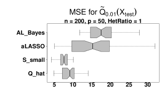
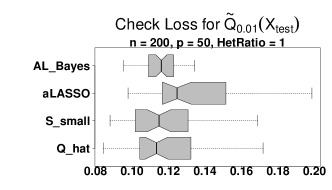
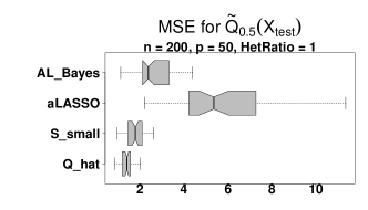
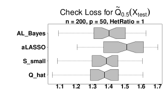
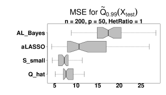
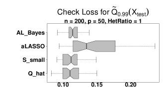
Figure 1: Quantile mean squared error (MSE; left) and check loss (right) among competing quantile regression methods; nonoverlapping notches indicate significant differences between medians, and the dashed vertical line (right) denotes $\tau$. The proposed approach ($\mbox{S}_{small}(\tau)$) offers substantial improvements in quantile prediction relative to both frequentist and Bayesian competitors, and matches or improves upon the model-based fitted quantiles ($\mbox{Q}_{hat}$).

Across all quantiles, the proposed approach demonstrates exceptional quantile prediction. The quantile MSEs for $\mbox{S}_{small}(\tau)$ are significantly lower than those for competing frequentist and Bayesian methods, especially for extreme quantiles near zero or one. $\mbox{S}_{small}(\tau)$ decisively outperforms aLASSO in check loss, even though aLASSO—unlike $\mbox{S}_{small}(\tau)$—directly optimizes (penalized) check loss via (2). Finally, the linear quantile predictions from $\mbox{S}_{small}(\tau)$ match or improve upon model-based fitted quantiles ($\mbox{Q}_{hat}$), despite the nonlinearity of the quantile functions in the model (21).

4.3 Uncertainty Quantification

Next, we assess uncertainty quantification for the posterior action (9) via 95% posterior interval estimates. Specifically, we construct intervals from the posterior draws of (9) for two subsets: the smallest acceptable subset $\mbox{S}_{small}(\tau)$ and the full set of covariates $\mbox{S}_{full}=\{1,\ldots,p\}$. By design, $\mbox{S}_{small}(\tau)$ is sparse, so the interval estimates under (9) for any covariates omitted from $\mbox{S}_{small}(\tau)$ are null. Since $\mbox{S}_{full}$ includes all covariates, it circumvents this issue. We compare these interval estimates to the 95% posterior credible intervals from $\mbox{AL}_{Bayes}$ for each $\tau$.

The intervals are evaluated for calibration, measured by the empirical coverage, and sharpness, measured by the average interval widths, in Table LABEL:covrates. Narrow intervals that achieve the 95% nominal coverage are preferred. Most notably, the posterior actions for both $\mbox{S}_{full}$ and $\mbox{S}_{small}(\tau)$ yield significantly more narrow intervals than $\mbox{AL}_{Bayes}$, often by a factor of 2-5. These effects are especially pronounced for extreme quantiles near zero or one, where $\mbox{AL}_{Bayes}$ is excessively conservative and underpowered. Importantly, both $\mbox{S}_{full}$ and $\mbox{S}_{small}(\tau)$ maintain the nominal coverage in nearly all settings. As expected, the sparsity of $\mbox{S}_{small}(\tau)$ produces the most narrow intervals, but also sacrifices empirical coverage for any active variables excluded from $\mbox{S}_{small}(\tau)$.

Table 3: $\boldsymbol{n=200,p=50,\textbf{\mbox{HetRatio}}=1}$

	$\tau$	0.01	0.05	0.1	0.25	0.5	0.75	0.90	0.95	0.99
Coverage Rate	$\mbox{S}_{small}(\tau)$	0.83	0.86	0.86	0.88	0.90	0.88	0.86	0.85	0.83
	$\mbox{S}_{full}$	0.98	0.97	0.97	0.95	0.94	0.95	0.96	0.97	0.97
	$\mbox{AL}_{Bayes}$	0.98	0.97	0.96	0.94	0.94	0.95	0.96	0.97	0.98
Avg. 95% CI Width	$\mbox{S}_{small}(\tau)$	1.23	1.13	1.10	0.94	0.81	0.94	1.10	1.17	1.27
	$\mbox{S}_{full}$	3.56	2.87	2.52	2.02	1.76	2.03	2.54	2.90	3.60
	$\mbox{AL}_{Bayes}$	8.64	4.95	3.97	3.10	2.73	3.04	3.95	4.99	9.19

$\boldsymbol{n=200,p=50,\textbf{\mbox{HetRatio}}=0.5}$

	$\tau$	0.01	0.05	0.1	0.25	0.5	0.75	0.90	0.95	0.99
Coverage Rate	$\mbox{S}_{small}(\tau)$	0.92	0.94	0.94	0.92	0.91	0.92	0.92	0.93	0.91
	$\mbox{S}_{full}$	0.97	0.97	0.96	0.95	0.95	0.95	0.96	0.96	0.97
	$\mbox{AL}_{Bayes}$	0.99	0.98	0.98	0.97	0.98	0.97	0.97	0.98	0.98
Avg. 95% CI Width	$\mbox{S}_{small}(\tau)$	1.02	0.95	0.89	0.81	0.77	0.80	0.88	0.94	1.02
	$\mbox{S}_{full}$	3.56	2.96	2.67	2.33	2.18	2.34	2.69	2.96	3.57
	$\mbox{AL}_{Bayes}$	7.87	4.30	3.43	2.62	2.33	2.61	3.43	4.34	8.30

Table 4: $\boldsymbol{n=500,p=20,\textbf{\mbox{HetRatio}}=1}$

	$\tau$	0.01	0.05	0.1	0.25	0.5	0.75	0.90	0.95	0.99
Coverage Rate	$\mbox{S}_{small}(\tau)$	0.92	0.91	0.91	0.90	0.89	0.89	0.92	0.94	0.95
	$\mbox{S}_{full}$	0.93	0.92	0.92	0.91	0.91	0.91	0.94	0.96	0.97
	$\mbox{AL}_{Bayes}$	0.94	0.94	0.94	0.93	0.94	0.95	0.98	0.99	0.99
Avg. 95% CI Width	$\mbox{S}_{small}(\tau)$	0.63	0.51	0.45	0.36	0.31	0.37	0.46	0.52	0.65
	$\mbox{S}_{full}$	1.41	1.14	1.01	0.83	0.75	0.84	1.02	1.15	1.43
	$\mbox{AL}_{Bayes}$	4.01	2.40	1.88	1.43	1.25	1.41	1.88	2.42	4.32

Table 5: $\boldsymbol{n=500,p=20,\textbf{\mbox{HetRatio}}=0.5}$

	$\tau$	0.01	0.05	0.1	0.25	0.5	0.75	0.90	0.95	0.99
Coverage Rate	$\mbox{S}_{small}(\tau)$	0.92	0.91	0.90	0.89	0.89	0.89	0.91	0.91	0.92
	$\mbox{S}_{full}$	0.93	0.92	0.92	0.91	0.90	0.91	0.92	0.92	0.94
	$\mbox{AL}_{Bayes}$	0.95	0.95	0.95	0.94	0.94	0.95	0.96	0.96	0.98
Avg. 95% CI Width	$\mbox{S}_{small}(\tau)$	0.39	0.34	0.31	0.28	0.26	0.29	0.31	0.34	0.38
	$\mbox{S}_{full}$	1.54	1.29	1.19	1.05	0.99	1.05	1.19	1.30	1.54
	$\mbox{AL}_{Bayes}$	3.71	2.15	1.69	1.29	1.13	1.26	1.68	2.19	4.00

Coverage rates and average widths of 95% credible intervals for the posterior action (9) with $\mbox{S}_{small}(\tau)$ or $\mbox{S}_{full}$ as well as $\mbox{AL}_{Bayes}$. The intervals for $\mbox{S}_{small}(\tau)$ and $\mbox{S}_{full}$ are significantly more narrow than those for $\mbox{AL}_{Bayes}$, especially for quantiles near zero or one, and typically maintain nominal coverage. $\mbox{S}_{small}(\tau)$ sacrifices some coverage in favor of sparsity, and thus provides the most narrow intervals.

4.4 Selection

We evaluate quantile-specific subset selection by computing true positive rates (TPR) and true negative rates (TNR) for the variables selected by $\mbox{S}_{small}(\tau)$, aLASSO and $\mbox{AL}_{Bayes}$. Here, $\mathcal{M}$ is not a competitor: it does not specify linear quantiles or any mechanism for quantile-specific variable selection. The results are presented in Table LABEL:Table1.

Across all settings, $\mbox{S}_{small}(\tau)$ provides a superior balance between TPR and TNR. $\mbox{AL}_{Bayes}$ is underpowered and overconservative due to the excessively wide posterior credible intervals that are used for selection (see Table LABEL:covrates). The frequentist competitor aLASSO often produces similar TPRs but lower TNRs compared to $\mbox{S}_{small}(\tau)$, and thus selects too many variables.

Improvements in TPRs for $\mbox{S}_{small}(\tau)$ over aLASSO are most notable for extreme quantiles, though $\mbox{S}_{small}(\tau)$ appears to offer relatively low power in the larger $p$ settings. Considering this exception more carefully, the coefficients $\beta_{het}^{*}(.01)$ and $\beta_{het}^{*}(.99)$ are about four times larger in magnitude than $\boldsymbol{\beta}_{hom}^{*}(\tau)$, so that $\boldsymbol{X}_{het}\beta_{het}^{*}(\tau)$ explains the vast majority of the variability in the quantiles for $\tau\in\{0.01,0.99\}$. For these quantiles, $\mbox{S}_{small}(\tau)$ always includes the heterogeneous predictor, but leaves out the homogeneous predictors, which are less important for predicting those quantiles. This is consistent with the definition of $\mbox{S}_{small}(\tau)$, which seeks to find the smallest subset that nearly matches the model-based quantile estimation from $\mathcal{M}$, and indeed achieves this latter objective (Figure 1).

Table 4: $\boldsymbol{n=200,p=50,\textbf{\mbox{HetRatio}}=1}$

	$\tau$	0.01	0.05	0.1	0.25	0.5	0.75	0.90	0.95	0.99
TPR	$\mbox{S}_{small}(\tau)$	0.43	0.54	0.61	0.69	0.79	0.63	0.63	0.57	0.46
	aLASSO	0.21	0.76	0.85	0.89	0.95	0.89	0.82	0.71	0.27
	$\mbox{AL}_{Bayes}$	0.00	0.02	0.09	0.22	0.35	0.23	0.08	0.03	0.00
TNR	$\mbox{S}_{small}(\tau)$	0.88	0.85	0.83	0.82	0.84	0.83	0.84	0.85	0.87
	aLASSO	0.88	0.55	0.39	0.29	0.27	0.28	0.38	0.54	0.83
	$\mbox{AL}_{Bayes}$	0.97	0.97	0.97	0.97	0.96	0.97	0.95	0.97	0.93

$\boldsymbol{n=200,p=50,\textbf{\mbox{HetRatio}}=0.5}$

	$\tau$	0.01	0.05	0.1	0.25	0.5	0.75	0.90	0.95	0.99
TPR	$\mbox{S}_{small}(\tau)$	0.77	0.88	0.90	0.92	0.97	0.91	0.88	0.86	0.78
	aLASSO	0.18	0.87	0.93	0.97	0.98	0.97	0.92	0.86	0.29
	$\mbox{AL}_{Bayes}$	0.00	0.00	0.06	0.30	0.50	0.31	0.05	0.01	0.00
TNR	$\mbox{S}_{small}(\tau)$	0.88	0.86	0.84	0.81	0.80	0.81	0.84	0.86	0.88
	aLASSO	0.92	0.59	0.41	0.32	0.32	0.32	0.41	0.57	0.88
	$\mbox{AL}_{Bayes}$	0.97	0.97	0.96	0.96	0.96	0.97	0.97	0.97	0.97

Table 5: $\boldsymbol{n=500,p=20,\textbf{\mbox{HetRatio}}=1}$

	$\tau$	0.01	0.05	0.1	0.25	0.5	0.75	0.90	0.95	0.99
TPR	$\mbox{S}_{small}(\tau)$	0.96	0.98	0.98	0.95	1.00	0.92	0.98	0.99	0.96
	aLASSO	0.65	0.99	1.00	0.99	1.00	0.98	0.99	0.99	0.72
	$\mbox{AL}_{Bayes}$	0.00	0.31	0.73	0.83	0.99	0.86	0.73	0.36	0.00
TNR	$\mbox{S}_{small}(\tau)$	0.94	0.93	0.93	0.93	0.91	0.92	0.92	0.93	0.94
	aLASSO	0.87	0.71	0.64	0.58	0.52	0.55	0.63	0.72	0.82
	$\mbox{AL}_{Bayes}$	1.00	1.00	1.00	0.99	0.99	0.99	0.99	1.00	1.00

Table 6: $\boldsymbol{n=500,p=20,\textbf{\mbox{HetRatio}}=0.5}$

	$\tau$	0.01	0.05	0.1	0.25	0.5	0.75	0.90	0.95	0.99
TPR	$\mbox{S}_{small}(\tau)$	0.88	0.88	0.87	0.85	1.00	0.84	0.88	0.87	0.86
	aLASSO	0.77	0.96	0.97	0.96	1.00	0.94	0.96	0.97	0.77
	$\mbox{AL}_{Bayes}$	0.80	0.87	0.89	0.86	0.99	0.84	0.88	0.89	0.82
TNR	$\mbox{S}_{small}(\tau)$	0.97	0.95	0.94	0.92	0.90	0.91	0.94	0.95	0.97
	aLASSO	0.81	0.71	0.63	0.57	0.57	0.56	0.59	0.77	0.86
	$\mbox{AL}_{Bayes}$	1.00	1.00	1.00	1.00	0.99	0.99	0.99	1.00	1.00

True positive rates (TPR) and true negative rates (TNR) for variable selection averaged across simulations. The proposed approach ($\mbox{S}_{small}(\tau)$) neatly balances TPR and TNR. The Bayesian competitor ($\mbox{AL}_{Bayes}$) is significantly underpowered due to excessively wide posterior credible intervals, while the frequentist competitor (aLASSO) often overselects variables (low TNRs).

4.5 Quantile Crossing

Lastly, we investigate the quantile crossing properties of the competing approaches. Under a coherent probability model for $Y\mid\boldsymbol{x}$, quantiles cannot cross: $\tilde{Q}_{\tau}(\boldsymbol{x})<\tilde{Q}_{\tau^{\prime}}(\boldsymbol{x})$ for any $\tau<\tau^{\prime}$. However, only the model-based quantiles ($\mbox{Q}_{hat}$) enforce this property; the competing methods, including the proposed approach, do not explicitly enforce quantile non-crossing. Thus, we seek to quantify the abundance of quantile non-crossing for each method.

For any $\tau<\tau^{\prime}$, we compute the out-of-sample non-crossing rate (NCR) between neighboring quantile predictions at the testing points:

$$\mbox{NCR}(\tau,\tau^{\prime})=n_{test}^{-1}\sum_{i=1}^{n_{test}}\mathbbm{1}\{\tilde{Q}_{\tau}(\boldsymbol{x}_{test_{i}})<\tilde{Q}_{\tau^{\prime}}(\boldsymbol{x}_{test_{i}})\}.$$ (22)

When $\mbox{NCR}(\tau,\tau^{\prime})=1$, there is no quantile crossing between the $\tau$th and $\tau^{\prime}$th quantiles.

We compute $\mbox{NCR}(0.01,0.05)$ and $\mbox{NCR}(0.95,0.99)$ averaged across simulations for each method (Table 7). Remarkably, the proposed approach renders quantile crossing negligible without any explicit constraints in the decision analysis for estimation or selection. These results showcase a key advantage of the Bayesian decision analysis (6): by fitting to the model-based fitted quantiles via (8), the optimal linear actions benefit from the implicit quantile non-crossing of $\hat{Q}_{\tau}(\boldsymbol{x})$ under $\mathcal{M}$. Thus, we (nearly) acquire the primary advantage of simultaneous quantile regression methods (Section 1.2), but without the need for unwieldy constraints. By comparison, the competing frequentist approach is subject to abundant quantile crossing, especially with larger $p$ and stronger heterogeneity. The Bayesian competitor preserves non-crossing, but is generally inaccurate in its predictions (Figure 1). For both methods, this limits the interpretability of the estimated linear coefficients and suggests that the estimated quantiles may be unreliable for prediction or inference.

Table 7: $\boldsymbol{n=200,p=50,\textbf{\mbox{HetRatio}}=1}$

	$\mbox{NCR}(0.01,0.05)$	$\mbox{NCR}(0.95,0.99)$
$\mbox{S}_{small}(\tau)$	0.99	0.99
$\mbox{AL}_{Bayes}$	0.99	0.99
aLASSO	0.72	0.79

$\boldsymbol{n=200,p=50,\textbf{\mbox{HetRatio}}=0.5}$

	$\mbox{NCR}(0.01,0.05)$	$\mbox{NCR}(0.95,0.99)$
$\mbox{S}_{small}(\tau)$	0.99	0.98
$\mbox{AL}_{Bayes}$	0.99	0.99
aLASSO	0.75	0.79

$\boldsymbol{n=500,p=20,\textbf{\mbox{HetRatio}}=1}$

	$\mbox{NCR}(0.01,0.05)$	$\mbox{NCR}(0.95,0.99)$
$\mbox{S}_{small}(\tau)$	0.997	1.00
$\mbox{AL}_{Bayes}$	0.99	0.99
aLASSO	0.95	0.94

$\boldsymbol{n=500,p=20,\textbf{\mbox{HetRatio}}=0.5}$

	$\mbox{NCR}(0.01,0.05)$	$\mbox{NCR}(0.95,0.99)$
$\mbox{S}_{small}(\tau)$	1.00	1.00
$\mbox{AL}_{Bayes}$	0.99	1.00
aLASSO	0.95	0.94

Quantile non-crossing rates between the 1st and 5th and 95th and 99th quantiles. Unlike aLASSO, the proposed approach $\mbox{S}_{small}(\tau)$ renders quantile crossing a non-issue.

5 Quantile Estimation, Inference, and Selection for Educational Outcomes

Childhood educational outcomes are affected by adverse environmental exposures such as air quality and lead, and social stressors like poverty and racial residential isolation (Miranda et al., 2007). Using a large cohort of children in North Carolina (CEHI, 2020), we analyze student-level 4th end-of-grade (EoG) reading test scores ($y_{i}$) along with individual birth information, mother/child demographics, air quality exposure, blood lead measurements, and socioeconomic factors ($\boldsymbol{x}_{i}$). The variables are summarised in Table 4. Previous analyses of these data have exclusively used homoscedastic mean regression for estimation and variable selection (Kowal et al., 2021; Kowal, 2022; Bravo et al., 2022). However, it is essential to know which, if any, of the environmental exposures, social stressors, or other factors are heterogeneous; i.e., to determine whether (any of) these effects vary in their impact on low, medium, or high-achieving students. Thus, quantile regression is an informative tool—especially with the ability to quantify effect directions and magnitudes, measure and report uncertainty, and provide quantile-specific subset selection.

Birth information
mEdu	Mother’s education group at the time of birth (No high school diploma, High school diploma, College diploma)
mRace	Mother’s race/ethnicity group (Non-Hispanic (NH) White, NH Black)
BWTpct	Birthweight percentile
mAge	Mother’s age at the time of birth
Male	Male infant? (1 = Yes)
Smoker	Mother smoked? (1 = Yes)
NotMarried	Not married at time of birth (1 = Yes)
NOPNC	Mother received pre-natal care before birth? (1 = No prenatal care)
Weeks_Gestation	Gestational period (in weeks)
Education/End-of-grade (EoG) test information
Reading_Score	Standardized score for the (chronologically first) 4th EoG reading test
Blood lead surveillance
Blood_lead	Blood lead level (micrograms per deciliter)
Social/Economic status
EconDisadvantage	Economically disadvantaged students are indicated by participation in the free/reduced price lunch program (1 = Participation in the program)
NDI	Neighborhood Deprivation Index, at time of EoG test
RI	Residential isolation, at time of EoG test

Table 4: Variables in the North Carolina dataset. Data are restricted to children with non-Hispanic Black or non-Hispanic White mothers (Bravo et al., 2022), 30-42 weeks of gestation, 0-104 weeks of age-within-cohort, mother’s age 15-44, Blood_Lead $\leq$ 10, birth order $\leq$ 4, no current limited English proficiency, and residence in NC at the time of birth and the time of 4th EoG test. Numeric covariates are centered and scaled to mean zero and standard deviation 0.5.

We augment the covariates in Table 4 with interactions between mother’s race (mRace) and each of blood lead level (blood_lead), neighborhood deprivation (NDI), and racial residential isolation (RI). Crucially, these interactions allow us to assess whether the (possibly heterogeneous) effects of environmental exposures and social stressors on educational outcomes also differ between race groups.

We fit the Bayesian LL-LS model (21) to this dataset of $n=$ 23,232 students with $p=$ 18 covariates. Posterior and posterior predictive diagnostics (Gelman, Meng and Stern, 1996) demonstrate that the model is well-calibrated to the data, and notably provide key evidence for heteroscedasticity of $Y\mid\boldsymbol{x}$ (see the supplementary material). Thus, we anticipate that quantile regression may detect heterogeneous covariate effects.

Quantile-specific acceptable families $\mathbbm{A}_{\varepsilon}(\tau)$ are constructed for $\tau\in\{0.01,0.05,0.25,0.5,0.75,0.95,0.99\}$ under $\mathcal{M}$ using the subset search and selection techniques from Sections 2-3. Many of the demographic and socioeconomic covariates (Table 4) are strongly correlated. As a result, there are likely many subsets that perform similarly—which is captured by the acceptable family $\mathbbm{A}_{\varepsilon}(\tau)$, but not any single ”best” subset. In particular, we identify several hundred acceptable subsets for each $\tau$. We summarize the acceptable family $\mathbbm{A}_{\varepsilon}(\tau)$ using quantile-specific coefficient estimations and intervals for $\mbox{S}_{small}(\tau)$ along with the quantile-specific variable importance (19). For comparison, we include point estimates from aLASSO and posterior means and 95% credible intervals from $\mbox{AL}_{Bayes}$ for the quantile-specific linear coefficients.

In Figure 2 we report the estimates and uncertainty quantification among the competing methods for the main effects that do not include interactions with race. Some of the covariates are not selected by $\mbox{S}_{small}(\tau)$ or aLASSO for certain quantiles, so the resulting point estimates (and intervals for $\mbox{S}_{small}(\tau)$) are fixed at zero. The variables Weeks_Gestation and NOPNC do not belong to $\mbox{S}_{small}(\tau)$ for any $\tau$, and thus are omitted.

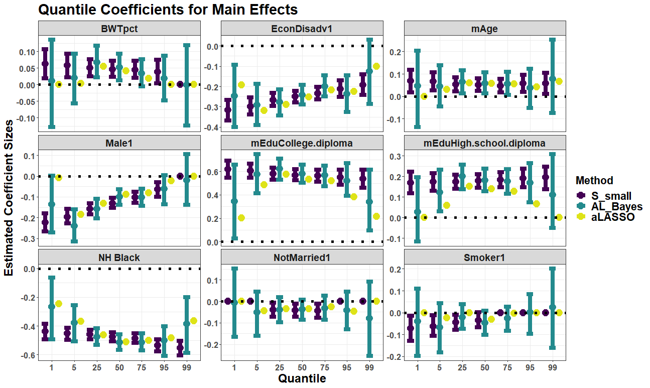
Figure 2: Quantile-specific point estimates and 95% credible intervals for main effects (not interacted with mother’s race) under $\mbox{S}_{small}$ (purple), $\mbox{AL}_{Bayes}$ (green) and aLASSO (yellow); the horizontal line denotes zero. Under the proposed approach ($\mbox{S}_{small}$), we identify several heterogeneous effects on reading scores, including gender and economically disadvantaged students. Other effects, such birthweight percentile and mother’s age, are relatively homogeneous. By contrast, $\mbox{AL}_{Bayes}$ exhibits excessively wide credible intervals, especially for extreme quantiles, while the aLASSO estimates are highly variable and nonsmooth across $\tau$.

The magnitude and direction of the coefficient estimates from $\mbox{S}_{small}$ reveal numerous interesting patterns. First, the point estimates for EconDisadv and Male are negative across all quantiles, but the effects on reading scores are more pronounced for lower quantiles. This suggests that the discrepancies between male and female students, and between students who are economically disadvantaged and students who are not, are greater for lower-scoring students. Other covariates have little variability over $\tau$; the coefficients for BWTpct and mAge are relatively flat, demonstrating that birthweight percentile and mother’s age at the time of birth have significant, yet homogeneous impacts across the distribution of $Y\mid\boldsymbol{x}$.

The 95% credible intervals for the coefficients in $\mbox{S}_{small}(\tau)$ are substantially more narrow than $\mbox{AL}_{Bayes}$, which is consistent with the simulation results (Section 4.4). This advantage is most pronounced in the extreme quantiles near zero or one, and helps to uncover clear patterns in covariate heterogeneity. The aLASSO estimates vary erratically across $\tau$, often with large jumps for extreme quantiles. This effect is notable for the Male coefficients: the estimated coefficients are increasingly negative for smaller $\tau$, yet the estimate at $\tau=0.01$ is zero. Similar patterns persist for mEdu, EconDisadv and mRace, and undermine the interpretability of the quantile-specific coefficients under aLASSO.

The main and race-interaction effects for the social stressors and environmental exposures are presented in Figure 3. Here, the main effects refer specifically to the NH White group, while the interaction effects refer to the differences between these effects for NH Black students and NH White students. First, lead exposure is especially detrimental for lower-scoring students, with no estimated differences between the race groups. Second, the estimated RI effect is similarly detrimental for lower-scoring students, but only for NH Black students. Finally, NDI exhibits a heterogeneous effect for NH White students, with increasingly negative effects for lower-scoring students. The positive and heterogenous effects for the NDI contrast term must be interpreted carefully: in conjunction with the main effect estimates, these estimates indicate that the effect of NDI is still negative for NH Black students, but now homogeneous across $\tau$.

Once again, $\mbox{AL}_{Bayes}$ produces excessively wide credible intervals, which obscures important heterogeneity patterns across $\tau$. Similarly, aLASSO only identifies nonzero effects for NDI among NH White students; yet even these estimated effects fail to satisfy monotonicity across $\tau$.

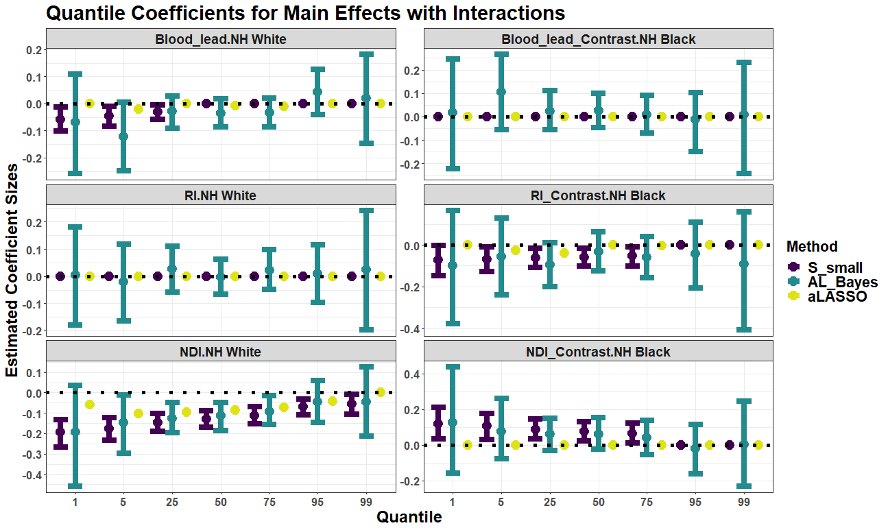
Figure 3: Quantile-specific point estimates and 95% credible intervals for social and environmental exposures that are interacted with mother’s race under $\mbox{S}_{small}$ (purple), $\mbox{AL}_{Bayes}$ (green) and aLASSO (yellow); the horizontal line denotes zero. The main effects (left) refer specifically to the NH White group, while the interaction effects (right) refer to the differences between these effects for NH Black students and NH White students. Under $\mbox{S}_{small}(\tau)$, the blood_lead effects are increasingly negative for $\tau<0.5$, with no clear differences between NH Black and NH White students. RI similarly exhibits an increasingly negative effect for lower quantiles, but only for NH Black students. Finally, the NDI effects are heterogeneous and increasingly negative for lower quantiles among NH White students, but for NH Black students, the effects are negative yet homogeneous across $\tau$. Again, $\mbox{AL}_{Bayes}$ produces excessively wide credible intervals, while aLASSO only identifies nonzero effects for NDI among NH White students.

Finally, we present the variable importance $\mbox{VI}_{j}(\tau)$ for each covariate $j$ and quantile $\tau$ in Figure 4. $\mbox{VI}_{j}(\tau)$ seeks to summarize the acceptable family $\mathbbm{A}_{\varepsilon}(\tau)$ of near-optimal subsets by tallying the proportion of acceptable subsets in which each variable belongs. In particular, we identify keystone covariates that satisfy $\mbox{VI}_{j}(\tau)>0.9$ for any $\tau$, and thus are valuable covariates that belong to at least 90% of acceptable subsets. t

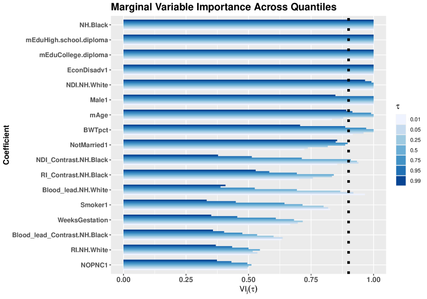
Figure 4: Variable importance $\mbox{VI}_{j}(\tau)$ from (19), colored by quantile; the dashed line indicates 0.90. Large values indicate that the covariate appears in many of the acceptable subsets. mEdu, mRace and EconDisadvantage appear in all acceptable subsets for all quantiles, while several of the environmental and social factors exhibit heterogeneous variable importance, often with increasing $\mbox{VI}_{j}(\tau)$ for smaller quantiles.

Most notably, mEdu, mRace and EconDisadvantage appear in all acceptable subsets across quantiles. These keystone covariates are essential for near-optimal prediction across the entire distribution of reading scores $Y\mid\boldsymbol{x}$. Heterogeneous and large $\mbox{VI}_{j}(\tau)$ effects are apparent for blood_lead main effects (i.e., for NH White students) and NDI and RI contrasts (i.e., differences between NH Black and NH White students), with increasing variable importance for lower quantiles. Similarly heterogeneous and large variable importance are observed for mAge, BWTpct, and NotMarried.

In aggregate, our analysis uncovers substantial heterogeneity in the effects of environmental exposures, social stressors, and other key factors on reading scores. Notably, both the coefficient (point and interval) estimates (Figures 2-3) and the variable importance (Figure 4) highlight numerous increasingly adverse effects for lower-scoring students. These effects include lead exposure, economic disadvantagement, racial residential isolation, and neighborhood deprivation, among others, with some differential effects by race. These new findings contribute to our understanding of the disparities in childhood development and educational outcomes.

6 Conclusion

We proposed a novel approach to Bayesian linear quantile regression with subset selection. The procedure features two stages, but operates within a single, coherent, Bayesian modeling and decision analysis framework. First, the analyst curates a Bayesian regression model to best represent the conditional distribution $Y\mid\boldsymbol{x}$. Then, based on the conditional quantiles from the Bayesian model, we apply a decision analysis to extract linear and quantile-specific coefficient estimates, uncertainty quantification, and subset selection. This approach uses a quantile-focused squared error loss function, which maintains a close, theoretical connection to density regression on the Wasserstein geometry. Crucially, this loss function enables closed-form computation of optimal linear coefficients and uncertainty quantification for any subset of predictors. We leverage these computational results to unlock state-of-the-art subset search and selection algorithms that were previously available only for mean regression. Our strategy prioritizes accumulation of many, highly predictive subsets to form a quantile-specific acceptable family, which we summarize by reporting the smallest acceptable subset (in accordance with the parsimony principle) and measures of variable importance.

There are several advantages of the proposed approach relative to existing frequentist and Bayesian quantile regression methods. First, the framework is valid under any Bayesian regression model. Thus, the analyst can prioritize calibrated modeling of the observed data without the need to accommodate quantile-specific modeling requirements, such as inadequate likelihoods or unwieldy constraints. Second, the decision analysis conveys regularization, uncertainty quantification, and smoothness across quantiles from the underlying Bayesian regression model. This occurs despite the fact that the decision analysis is applied separately for each quantile, yielding straightforward and efficient implementations. Finally, our approach delivers subset search and selection for quantile regression, which has remained elusive among frequentist and Bayesian methods.

These benefits translate to significant empirical improvements. In an extensive simulation study, we found that the proposed approach produces more accurate quantile predictions, more precise (yet calibrated) uncertainty quantification, and more powerful variable selection for quantile regression coefficients.

We applied our methods to analyze the effects of environmental exposures, social stressors, and other key factors on 4th end-of-grade reading test scores for a large cohort of children in North Carolina. Our analysis revealed several important and unique insights into educational inequities. Most notably, we found that lead exposure, economic disadvantagement, racial residential isolation, and neighborhood deprivation more adversely impact reading test scores for lower-scoring students. These effects exhibited heterogeneity not only across quantiles, but also across race groups. These alarming results have important implications for childhood development and educational outcomes, and may inform policy to develop and target intervention strategies.

With such encouraging results, there are numerous promising directions for future research. Although we have focused on linear quantile regression, our decision analysis framework can be readily extended to nonlinear quantile-specific summaries, such as trees or additive models. This enhanced flexibility may be useful for quantile estimation under nonlinear Bayesian models, such as heteroscedastic Bayesian additive regression trees (Pratola et al., 2020). Further, our approach is not limited to Bayesian models with Gaussian errors. A useful extension would be to consider Bayesian models for extreme events (Fagnant et al., 2020), with a customized decision analysis for estimation, uncertainty quantification, and selection. Finally, the proposed (linear) quantile predictions are quick to compute with minimal storage requirements, and thus may be used to provide fast, model-based prediction intervals, especially when the underlying Bayesian model does not admit efficient posterior predictive sampling.

[Acknowledgments] The findings and conclusions in this presentation or publication are those of the authors and do not necessarily represent the views of the North Carolina Department of Health and Human Services, Division of Public Health, the National Institutes of Health, the Army Research Office, or the U.S. Government. The U.S. Government is authorized to reproduce and distribute reprints for Government purposes notwithstanding any copyright notation herein.

Research reported in this publication was supported by the National Institute of Environmental Health Sciences of the National Institutes of Health under award number R01ES028819, National Science Foundation under award number SES-2214726, and the Army Research Office under award number W911NF-20-1-0184.

Supplement A A detailed expansion of Algorithm 1 for Bayesian quantile regression and subset selection, full Bayesian model specification for (21) used in the simulation and real data analysis, and additional simulation results. Supplement B An R package, QRSubsets, implementing the proposed methods is available online: https://github.com/jfeldman396/QRSubsets

References

- Alhamzawi, Yu and Benoit (2012) {barticle}[author] \bauthor\bsnmAlhamzawi, \bfnmRahim\binitsR., \bauthor\bsnmYu, \bfnmKeming\binitsK. and \bauthor\bsnmBenoit, \bfnmDries F\binitsD. F. (\byear2012). \btitleBayesian adaptive Lasso quantile regression. \bjournalStatistical Modelling \bvolume12 \bpages279–297. \endbibitem
- Bassett and Chen (2002) {barticle}[author] \bauthor\bsnmBassett, \bfnmGilbert W\binitsG. W. and \bauthor\bsnmChen, \bfnmHsiu-Lang\binitsH.-L. (\byear2002). \btitlePortfolio style: Return-based attribution using quantile regression. \bjournalEconomic applications of quantile regression \bpages293–305. \endbibitem
- Belloni and Chernozhukov (2011) {barticle}[author] \bauthor\bsnmBelloni, \bfnmAlexandre\binitsA. and \bauthor\bsnmChernozhukov, \bfnmVictor\binitsV. (\byear2011). \btitleL1-penalized quantile regression in high-dimensional sparse models. \bjournalThe Annals of Statistics \bvolume39 \bpages82 – 130. \bdoi10.1214/10-AOS827 \endbibitem
- Benoit and Van den Poel (2017) {barticle}[author] \bauthor\bsnmBenoit, \bfnmDries F\binitsD. F. and \bauthor\bparticleVan den \bsnmPoel, \bfnmDirk\binitsD. (\byear2017). \btitlebayesQR: A Bayesian approach to quantile regression. \bjournalJournal of Statistical Software \bvolume76 \bpages1–32. \endbibitem
- Bertsimas, King and Mazumder (2016) {barticle}[author] \bauthor\bsnmBertsimas, \bfnmDimitris\binitsD., \bauthor\bsnmKing, \bfnmAngela\binitsA. and \bauthor\bsnmMazumder, \bfnmRahul\binitsR. (\byear2016). \btitleBest subset selection via a modern optimization lens. \bjournalThe Annals of Statistics \bvolume44 \bpages813 – 852. \bdoi10.1214/15-AOS1388 \endbibitem