IRKA is a Riemannian Gradient Descent Method

Abstract

The iterative rational Krylov algorithm (IRKA) is a commonly used fixed-point iteration developed to minimize the $\mathcal{H}_{2}$ model order reduction error. In this work, IRKA is recast as a Riemannian gradient descent method with a fixed step size over the manifold of rational functions having fixed degree. This interpretation motivates the development of a Riemannian gradient descent method utilizing as a natural extension variable step size and line search. Comparisons made between IRKA and this extension on a few examples demonstrate significant benefits.

Keywords model order reduction, $\mathcal{H}_{2}$ norm, Riemannian optimization

1 Introduction

The iterative rational Krylov algorithm (IRKA) is a commonly used method for $\mathcal{H}_{2}$-optimal model order reduction (MOR) of linear time-invariant systems [GAB06, GAB08, ABG10]. It is principally a fixed point iteration based on interpolatory $\mathcal{H}_{2}$-optimality conditions; we describe it in Section 2.

Notably, there have also been approaches for $\mathcal{H}_{2}$ MOR via Riemannian optimization over certain matrix manifolds. Some have been based on Grassmann or Stiefel manifolds [YL99, XZ13, XJY15, XJY17, YJ17, WJ18, JW19, JX19, XJ19, YJX19, JX20, JX21, WJ22, XJ22]; others have used other matrix manifolds [SS15, SS16, Sat17b, Sat17a, Sat18, SS18, Sat19, LJX22].

In this work, we recast IRKA as a Riemannian optimization strategy over the manifold of stable rational functions of fixed McMillan degree $\Sigma_{r,m,p}^{-}(\mathbb{C})$, embedded in the Hardy space $\mathcal{H}_{2}$. We develop a geometric framework for IRKA (Section 6.2) and show that it can be interpreted as a Riemannian gradient descent method with a fixed step size (Section 7). Building on this observation, we introduce an extension having variable step size (Section 8) and present numerical experiments for this extended approach in Section 9.

These key results depend on the observation that the set of stable rational functions of fixed McMillan degree $\Sigma_{r,m,p}^{-}(\mathbb{C})$ is an embedded submanifold in the Hardy space $\mathcal{H}_{2}$. We prove this while also drawing out issues related to connectedness of the manifold and the Cauchy index. An accessible reference for these facts in the continuous-time case was not known to us. This framework allows a new geometric interpretation of IRKA as a Riemannian optimization method with fixed step size. This in turn leads to the introduction of an enhanced approach utilizing a backtracking line search that preserves stability, and guarantees a decrease in the $\mathcal{H}_{2}$ error at each step. Significantly, the utilization of different step sizes can be interpreted as a fixed point iteration with an equivalent set of interpolatory conditions.

We begin with a background on $\mathcal{H}_{2}$-optimal MOR and Riemann optimization in Sections 2 and 3, respectively. We then discuss known results on the manifold structure of $\Sigma_{r,m,p}^{-}(\mathbb{C})$ and introduce the new result for continuous-time systems in Section 4. This allows us to interpret the $\mathcal{H}_{2}$-optimal MOR problem as a Riemannian optimization problem in Section 5 and derive the Riemannian gradient of the $\mathcal{H}_{2}$ error. Then we give a geometric interpretation of necessary optimality conditions and IRKA in Section 6, leading to the interpretation of IRKA as a Riemannian gradient descent method with a fixed step size in Section 7. In Section 8, we introduce a variant of IRKA, Riemannian Gradient Descent IRKA (RGD-IRKA), which uses a variable step size to enforce stability preservation and decrease of the $\mathcal{H}_{2}$ error at every step. We compare the two methods in Section 9 and conclude with Section 10.

2 $\mathcal{H}_{2}$-optimal Model Order Reduction

We briefly describe IRKA and summarize relevant background and context for later discussion.

2.1 Model Order Reduction Problem

Given fom full-order model (FOM) of order $n$

$$E\dot{x}(t) =Ax(t)+Bu(t),\ x(0)=0,$$

$$y(t) =Cx(t),$$

the goal is to find rom reduced-order model (ROM) of order $r$

$$\widehat{E}\dot{\widehat{x}}(t) =\widehat{A}\widehat{x}(t)+\widehat{B}u(t),\ \widehat{x}(0)=0,$$

$$\widehat{y}(t) =\widehat{C}\widehat{x}(t),$$

such that $r\ll n$ and the outputs $y(t),\widehat{y}(t)\in\mathbb{C}^{p}$ are close to one another when the systems are presented with the same input $u(t)\in\mathbb{C}^{m}$. Here, $x(t)\in\mathbb{C}^{n}$ is the full-order state and $\widehat{x}(t)\in\mathbb{C}^{r}$ is the reduced-order state; $E,A\in\mathbb{C}^{n\times n}$, $B\in\mathbb{C}^{n\times m}$, $C\in\mathbb{C}^{p\times n}$, $\widehat{E},\widehat{A}\in\mathbb{C}^{r\times r}$, $\widehat{B}\in\mathbb{C}^{r\times m}$, and $\widehat{C}\in\mathbb{C}^{p\times r}$. We assume $E$ and $\widehat{E}$ are invertible and that $E^{-1}A$ and $\widehat{E}^{-1}\widehat{A}$ are Hurwitz (their eigenvalues are in the open left half-plane). We develop and present theory for general complex systems. The case of real systems follow directly from our discussion and we add remarks when necessary to highlight the real case.

To measure the distance between $y$ and $\widehat{y}$, we use the transfer functions $H$ and $\widehat{H}$ of the FOM and ROM, respectively:

$$H(s)=C{(sE-A)}^{-1}B\quad\textnormal{and}\quad\widehat{H}(s)=\widehat{C}\left\lparen s\widehat{E}-\widehat{A}\right\rparen^{-1}\widehat{B}.$$

The $\mathcal{H}_{2}$ error is defined as

$$\left\lVert H-\widehat{H}\right\rVert_{\mathcal{H}_{2}}=\left\lparen\frac{1}{2\pi}\int_{-\infty}^{\infty}\left\lVert H(\boldsymbol{\imath}\omega)-\widehat{H}(\boldsymbol{\imath}\omega)\right\rVert_{\operatorname{F}}^{2}\operatorname{d\!}{\omega}\right\rparen^{1/2}.$$

A uniform bound on the output error can be formulated:

$$\left\lVert y-\widehat{y}\right\rVert_{\mathcal{L}_{\infty}}\leqslant\left\lVert H-\widehat{H}\right\rVert_{\mathcal{H}_{2}}\lVert u\rVert_{\mathcal{L}_{2}}.$$

This motivates reducing the $\mathcal{H}_{2}$ error, thus assuring the output error $\lVert y-\widehat{y}\rVert_{\mathcal{L}_{\infty}}$ to be small for bounded input energy. This leads one to the $\mathcal{H}_{2}$-optimal MOR problem

$$\operatorname*{minimize}_{\begin{subarray}{c}\widehat{H}\textnormal{ of order }r\\ \widehat{H}\textnormal{ stable}\end{subarray}}\quad\left\lVert H-\widehat{H}\right\rVert_{\mathcal{H}_{2}}.$$ (2.1)

2.2 Hardy Space

Under the assumptions made for the FOM and ROM, both $H$ and $\widehat{H}$ are elements of the Hardy space $\mathcal{H}_{2}=\mathcal{H}_{2}^{p\times m}(\mathbb{C}^{+})$, where $\mathbb{C}^{+}$ denotes the open right half-plane. $\mathcal{H}_{2}$ is a Hilbert space of analytic functions $F\colon\mathbb{C}^{+}\to\mathbb{C}^{p\times m}$ satisfying $\sup_{\xi>0}\int_{-\infty}^{\infty}\lVert F(\xi+\boldsymbol{\imath}\omega)\rVert_{\operatorname{F}}^{2}\operatorname{d\!}{\omega}<\infty$ with the inner product

$$\langle F,G\rangle_{\mathcal{H}_{2}}=\frac{1}{2\pi}\int_{-\infty}^{\infty}\operatorname{\mathsf{trace}}\lparen F(\boldsymbol{\imath}\omega)^{*}G(\boldsymbol{\imath}\omega)\rparen\operatorname{d\!}{\omega},$$

using extensions of $F$ and $G$ from $\mathbb{C}^{+}$ to $\overline{\mathbb{C}^{+}}$. We have particular interest in the real Hilbert space of real $p\times m$ transfer functions, $\Re\mathcal{H}_{2}\subset\mathcal{H}_{2}$,

$$\Re\mathcal{H}_{2}=\left\{H\in\mathcal{H}_{2}:\overline{H(s)}=H(\overline{s}),\forall s\in\mathbb{C}^{+}\right\}.$$

2.3 Interpolatory Necessary Conditions for Optimality

The following theorem gives necessary $\mathcal{H}_{2}$-optimality conditions when the ROM has simple poles (see, e.g., [ML67, ABG10]).

Theorem 2.1.

Let $H,\widehat{H}\in\Re\mathcal{H}_{2}$ be such that $\widehat{H}$ has the pole-residue form

$$\widehat{H}(s)=\sum_{i=1}^{r}\frac{c_{i}b_{i}^{*}}{s-\lambda_{i}},$$

where $\lambda_{i}$ are pairwise distinct. Let $\widehat{H}$ be an $\mathcal{H}_{2}$-optimal approximation for $H$ as in (2.1). Then for $i=1,2,\ldots,r$

$$H\left\lparen-\overline{\lambda_{i}}\right\rparen b_{i} =\widehat{H}\left\lparen-\overline{\lambda_{i}}\right\rparen b_{i},$$ (2.2a)

$$c_{i}^{*}H\left\lparen-\overline{\lambda_{i}}\right\rparen =c_{i}^{*}\widehat{H}\left\lparen-\overline{\lambda_{i}}\right\rparen,$$ (2.2b)

$$c_{i}^{*}H^{\prime}\left\lparen-\overline{\lambda_{i}}\right\rparen b_{i} =c_{i}^{*}\widehat{H}^{\prime}\left\lparen-\overline{\lambda_{i}}\right\rparen b_{i}.$$ (2.2c)

That is, the $\mathcal{H}_{2}$-optimal ROMs are bitangential Hermite interpolants at reflected poles of the ROM in tangent directions given by the (vector) residues of the ROM. This theorem directly extends from $\Re\mathcal{H}_{2}$ to $\mathcal{H}_{2}$ as well.

2.4 Bitangential Hermite Interpolation

Given interpolation points $\sigma_{i}\in\mathbb{C}$ and tangential directions $b_{i}\in\mathbb{C}^{m}$, $c_{i}\in\mathbb{C}^{p}$, for $i=1,2,\ldots,r$, bitangential Hermite interpolants can be constructed via Petrov-Galerkin projection based on rational Krylov subspaces [GAB06]: For $H(s)=C{(sE-A)}^{-1}B$, define projection matrices, $V,W\in\mathbb{C}^{n\times r}$, such that

$$\operatorname{\mathsf{Im}}\lparen V\rparen =\operatorname{\mathsf{span}}\left\{\left\lparen\sigma_{i}E-A\right\rparen^{-1}Bb_{i}\right\}_{i=1}^{r},$$ (2.3a)

$$\operatorname{\mathsf{Im}}\lparen W\rparen =\operatorname{\mathsf{span}}\left\{\left\lparen\sigma_{i}E-A\right\rparen^{-*}C^{*}c_{i}\right\}_{i=1}^{r}$$ (2.3b)

($\operatorname{\mathsf{Im}}\lparen M\rparen$ denotes the image or range of $M$). Then rom ROM is constructed as

$$\widehat{E}=W^{*}EV,\ \widehat{A}=W^{*}AV,\ \widehat{B}=W^{*}B,\ \widehat{C}=CV.$$ (2.4)

For $\widehat{H}(s)=\widehat{C}{(s\widehat{E}-\widehat{A})}^{-1}\widehat{B}$, assuming invertibility where needed, we have for $i=1,2,\ldots,r$ [ABG10]:

$$H(\sigma_{i})b_{i} =\widehat{H}(\sigma_{i})b_{i},$$

$$c_{i}^{*}H(\sigma_{i}) =c_{i}^{*}\widehat{H}(\sigma_{i}),$$

$$c_{i}^{*}H^{\prime}(\sigma_{i})b_{i} =c_{i}^{*}\widehat{H}^{\prime}(\sigma_{i})b_{i}.$$

Note that $V$ and $W$ can be computed from solutions to Sylvester equations as we discuss next. Given interpolation data $\{\sigma_{i},b_{i},c_{i}\}$, let the $i$th column of $V$ be ${(\sigma_{i}E-A)}^{-1}Bb_{i}$. This construction satisfies (2.3a). Then it directly follows that $V$ satisfies the Sylvester equation

$$AV-EV\Sigma+B\widetilde{R}^{*}=0,$$

where $\Sigma=\operatorname{\mathsf{diag}}\lparen\sigma_{i}\rparen$ and the $i$th row of $\widetilde{R}$ is $b_{i}^{*}$. Then, for any invertible $T,\widetilde{E}\in\mathbb{C}^{r\times r}$, we have

$$\left\lparen AVTT^{-1}-EVTT^{-1}\Sigma+B\widetilde{R}^{*}\right\rparen T\widetilde{E}^{*}=0.$$

Therefore,

$$A(VT)\widetilde{E}^{*}+E(VT)\left\lparen-T^{-1}\Sigma T\widetilde{E}^{*}\right\rparen+B\left\lparen\widetilde{R}^{*}T\widetilde{E}^{*}\right\rparen=0.$$

Setting $\widetilde{V}=VT$, $\widetilde{A}=-\widetilde{E}T^{*}\Sigma^{*}T^{-*}$, and $\widetilde{B}=\widetilde{E}T^{*}\widetilde{R}$, we obtain

$$A\widetilde{V}\widetilde{E}^{*}+E\widetilde{V}\widetilde{A}^{*}+B\widetilde{B}^{*}=0.$$ (2.5)

Note that $\operatorname{\mathsf{Im}}\lparen\widetilde{V}\rparen=\operatorname{\mathsf{Im}}\lparen V\rparen$ and $\widetilde{E}^{-1}\widetilde{A}$ has $-\overline{\sigma_{i}}$ as eigenvalues. Analogous constructions hold for $W$, thus, as claimed, both $V$ and $W$ can be constructed from solving Sylvester equations of the form (2.5). This fact will be employed in the algorithmic development in Section 8.

Assuming that the interpolation data is closed under conjugation, $V$ and $W$ can be chosen to be real so that the ROM is also real. See [ABG20] for further details.

2.5 The IRKA Iteration

This interpolatory framework led to the development of the iterative rational Krylov algorithm (IRKA) [GAB06, GAB08, ABG10], a fixed point iteration algorithm that, given an iterate $\widehat{H}_{k}(s)=\sum_{i=1}^{r}\frac{c_{i}^{(k)}\left\lparen b_{i}^{(k)}\right\rparen^{*}}{s-\lambda_{i}^{(k)}}$, determines the next iterate $\widehat{H}_{k+1}$ from the interpolation conditions, for $i=1,2,\ldots,r$:

$$H\left\lparen-\overline{\lambda_{i}^{(k)}}\right\rparen b_{i}^{(k)} =\widehat{H}_{k+1}\left\lparen-\overline{\lambda_{i}^{(k)}}\right\rparen b_{i}^{(k)},$$ (2.6a)

$$\left\lparen c_{i}^{(k)}\right\rparen^{*}H\left\lparen-\overline{\lambda_{i}^{(k)}}\right\rparen =\left\lparen c_{i}^{(k)}\right\rparen^{*}\widehat{H}_{k+1}\left\lparen-\overline{\lambda_{i}^{(k)}}\right\rparen,$$ (2.6b)

$$\left\lparen c_{i}^{(k)}\right\rparen^{*}H^{\prime}\left\lparen-\overline{\lambda_{i}^{(k)}}\right\rparen b_{i}^{(k)} =\left\lparen c_{i}^{(k)}\right\rparen^{*}\widehat{H}_{k+1}^{\prime}\left\lparen-\overline{\lambda_{i}^{(k)}}\right\rparen b_{i}^{(k)}.$$ (2.6c)

Using Petrov-Galerkin projection as described in 2.4, these conditions uniquely determine a rational transfer function of order $r$. Then, this fixed point iteration, i.e., IRKA, is run until convergence upon which the ROM satisfies the interpolatory conditions (2.2). For details of IRKA, we refer the reader to [GAB08, ABG20]. Despite its success in practice and its usage across numerous applications, since IRKA is a fixed point iteration, the convergence and stability of the ROM are not theoretically guaranteed. In this work, by recasting IRKA in a Riemannian optimization setting, we develop efficient variants that resolve these issues.

3 Riemannian Optimization Background

We summarize here a few topics from Riemannian optimization (see also [AMS08, Bou23]), focusing in particular on Riemannian submanifolds (see, e.g., [Lan95, Lee12]), that will be used heavily in the rest of the paper.

3.1 General Manifolds

A (smooth) manifold $\mathcal{M}=(M,\mathcal{A})$, modeled on a Banach space $\mathbb{E}$, is a set $M$ together with an atlas $\mathcal{A}$, which is a collection of charts $(U_{i},\varphi_{i})$ ($i$ is an element of an index set) such that

1. each $U_{i}$ is a subset of $M$ and the $U_{i}$ cover $M$,

2. each $\varphi_{i}$ is a bijection from $U_{i}$ to an open subset $\varphi(U_{i})$ of $\mathbb{E}$ and $\varphi_{i}(U_{i}\cap U_{j})$ is open in $\mathbb{E}$ for any $i,j$,

3. the map $\varphi_{j}\circ\varphi_{i}^{-1}\colon\varphi_{i}(U_{i}\cap U_{j})\to\varphi_{j}(U_{i}\cap U_{j})$ is smooth (infinitely differentiable) for each pair of indices $i,j$.

We additionally assume that the atlas topology defined by the maximal atlas $\mathcal{A}^{+}$ (the collection of all charts compatible with elements of $\mathcal{A}$) is Hausdorff and second-countable. As is common in the literature, we conflate $\mathcal{M}$ with $M$ and $(U_{i},\varphi_{i})$ with $\varphi_{i}$ in the following.

The dimension of a manifold, denoted by $\dim(\mathcal{M})$, is defined to be $\dim(\mathbb{E})$. We are interested in both finite and infinite-dimensional manifolds. In particular, note that the Hardy space $\mathcal{H}_{2}$ is a manifold with $\mathbb{E}=\mathcal{H}_{2}$ and the identity map $\operatorname{id}\colon\mathcal{H}_{2}\to\mathcal{H}_{2}$ as the chart. Additionally, we are interested in embedded submanifolds (which we discuss in LABEL:{sec:embedsub}). But, first, we need a general concept of a smooth function and its differential.

3.2 General Tangent Space and Smooth Functions

A function $F\colon\mathcal{M}\to\mathcal{N}$ from a manifold $\mathcal{M}$ to a manifold $\mathcal{N}$ is smooth at $p$ if $\psi\circ F\circ\varphi^{-1}\colon\varphi(U)\to\psi(V)$ is smooth for a chart $(U,\varphi)$ of $\mathcal{M}$ and a chart $(V,\psi)$ of $\mathcal{N}$ such that $p\in U$ and $F(p)\in V$. A function is smooth if it is smooth at every point.

For a manifold $\mathcal{M}$ and point $p\in\mathcal{M}$, let $\mathcal{C}$ be the set of smooth curves $c\colon I\to\mathcal{M}$ such that $c(0)=p$ where $I\subseteq\mathbb{R}$ is an interval around zero. Define an equivalence relation $\sim$ between two curves $c_{1},c_{2}$ by

$$c_{1}\sim c_{2}\quad\Leftrightarrow\quad(\varphi\circ c_{1})^{\prime}(0)=(\varphi\circ c_{2})^{\prime}(0)$$

for some chart $\varphi$ of $\mathcal{M}$ around $p$. The tangent vectors of $\mathcal{M}$ at $p$ are then equivalence classes $[c]$ under the equivalence relation $\sim$. The tangent space of $\mathcal{M}$ at $p$, denoted $\mathrm{T}_{p}\mathcal{M}$, is the set of all tangent vectors at $p$, i.e., $\mathrm{T}_{p}\mathcal{M}=\mathcal{C}/{\sim}$. A tangent space is a vector space of the same dimension as the manifold.

The differential of a smooth function $F\colon\mathcal{M}\to\mathcal{N}$ at $p\in\mathcal{M}$ is the linear operator $DF(p)\colon\mathrm{T}_{p}\mathcal{M}\to\mathrm{T}_{F(p)}\mathcal{N}$ defined by

$$DF(p)[v]=[F\circ c],$$

where $c$ is a representative curve, i.e., $v=[c]\in\mathrm{T}_{p}\mathcal{M}$. Note that the brackets in $[v]$ in the above equation are only used to denote that $DF(p)$ is applied to $v$.

3.3 Embedded Submanifolds

A smooth immersion is a smooth mapping such that its differential is injective at each point and the image of the differential is a closed subspace. A smooth embedding is a smooth immersion that is also a homeomorphism onto its image, i.e., its inverse is continuous.

An embedded submanifold of $\overline{\mathcal{M}}$ is a subset $\mathcal{M}\subseteq\overline{\mathcal{M}}$ that is a manifold in the subspace topology, endowed with a smooth structure with respect to which the inclusion map $\mathcal{M}\hookrightarrow\overline{\mathcal{M}}$ is a smooth embedding. $\overline{\mathcal{M}}$ is called an ambient space.

For a function $F\colon\mathcal{M}\to\mathcal{N}$ between embedded submanifolds, smoothness is equivalent to the existence of a smooth extension of $F$ to an open neighborhood of $\mathcal{M}$ in its ambient space.

3.4 Tangent Vectors, Tangent Spaces, Tangent Bundle, and Normal Spaces of Embedded Submanifolds

Let $\mathcal{M}$ be an embedded submanifold of a Banach space $\mathbb{E}$. The tangent space of $\mathcal{M}$ at $p\in\mathcal{M}$ can be identified with the set of velocities at $p$ of all smooth curves in $\mathcal{M}$ going through $p$, i.e., $\mathrm{T}_{p}\mathcal{M}\simeq\{c^{\prime}(0)\mid c\colon I\to\mathcal{M},\ c(0)=p\}$, where $I\subseteq\mathbb{R}$ is any interval containing zero. In the following, we always interpret the tangent space of an embedded submanifold of a Banach space as a subset of the ambient space. Then, for every $p\in\mathcal{M}$, $\mathrm{T}_{p}\mathcal{M}$ forms a subspace of $\mathbb{E}$ of the same dimension as the dimension of the manifold.

The tangent bundle, denoted by $\mathrm{T}\mathcal{M}$, is a disjoint union of all tangent spaces of $\mathcal{M}$, in particular, $\mathrm{T}\mathcal{M}=\{(p,v)\mid p\in\mathcal{M}\text{ and }v\in\mathrm{T}_{p}\mathcal{M}\}$. The tangent bundle is itself a manifold of dimension $2\dim(\mathcal{M})$.

If $\mathbb{E}$ is additionally a Hilbert space, the normal space of $\mathcal{M}$ at $p\in\mathcal{M}$, denoted $\mathrm{N}_{p}\mathcal{M}$, is the orthogonal complement of the tangent space at $p$ in $\mathbb{E}$, i.e., $\mathrm{N}_{p}\mathcal{M}={(\mathrm{T}_{p}\mathcal{M})}^{\perp}$.

A scalar field over $\mathcal{M}$ is a function $f\colon\mathcal{M}\to\mathbb{R}$. A vector field over $\mathcal{M}$ is a function $X\colon\mathcal{M}\to\mathrm{T}\mathcal{M}$ such that $X(p)\in\mathrm{T}_{p}\mathcal{M}$ for all $p\in\mathcal{M}$.

3.5 Riemannian Manifolds and Submanifolds

A metric over $\mathcal{M}$ is a collection of inner products $\langle\cdot,\cdot\rangle_{p}$ over $\mathrm{T}_{p}\mathcal{M}$ for all $p\in\mathcal{M}$. A Riemannian metric is a metric $\langle\cdot,\cdot\rangle_{p}$ such that $p\mapsto\langle X(p),Y(p)\rangle_{p}$ is a smooth scalar field for all smooth vector fields $X,Y$. A Riemannian manifold is a manifold with a Riemannian metric.

A Riemannian submanifold is an embedded submanifold that inherits the Riemannian metric from the ambient manifold. Note that it is always possible for an embedded submanifold of a Riemannian manifold to inherit the metric because, if $\mathcal{M}\subseteq\overline{\mathcal{M}}$, then $\mathrm{T}_{p}\mathcal{M}\subseteq\mathrm{T}_{p}\overline{\mathcal{M}}$ for all $p\in\mathcal{M}$.

3.6 Riemannian Optimization

Now we have all the necessary background to summarize the basics of Riemannian optimization. A Riemannian optimization problem is an optimization problem of the form

$$\operatorname*{minimize}_{p\in\mathcal{M}}f(p),$$

where $\mathcal{M}$ is a Riemannian manifold and $f$ is a smooth scalar field. The gradient at $p\in\mathcal{M}$ of a smooth scalar field $f$ on a Riemannian manifold $\mathcal{M}$ is the unique tangent vector $\operatorname{grad}f(p)$ in $\mathrm{T}_{p}\mathcal{M}$ such that

$$Df(p)[v]=\langle\operatorname{grad}f(p),v\rangle_{p}$$

for all $v\in\mathrm{T}_{p}\mathcal{M}$. If $\mathcal{M}$ is a Riemannian submanifold of a Hilbert space $\mathbb{E}$, the gradient can be obtained via

$$\operatorname{grad}f(p)=\operatorname{Proj}_{p}\left\lparen\nabla\overline{f}(p)\right\rparen,$$ (3.1)

where $\operatorname{Proj}_{p}\colon\mathbb{E}\to\mathrm{T}_{p}\mathcal{M}$ is the orthogonal projector onto $\mathrm{T}_{p}\mathcal{M}$, $\overline{f}$ is a smooth extension of $f$ to an open neighborhood of $\mathcal{M}$ in $\mathbb{E}$, and $\nabla\overline{f}(p)$ is the Euclidean gradient of $\overline{f}$ at $p$.

As for Euclidean optimization, the necessary optimality condition for $p$ to be a local minimum is

$$\operatorname{grad}f(p)=0,$$ (3.2)

If $\mathcal{M}$ is an Riemannian submanifold, using (3.1), we have that the necessary optimality condition (3.2) is equivalent to

$$\nabla\overline{f}(p)\perp\mathrm{T}_{p}\mathcal{M}.$$ (3.3)

A step of Riemannian gradient descent takes the form

$$p_{k+1}=\mathrm{R}_{p_{k}}\left\lparen-\alpha_{k}\operatorname{grad}f(p_{k})\right\rparen,$$ (3.4)

where $\mathrm{R}_{p_{k}}\colon\mathrm{T}_{p_{k}}\mathcal{M}\to\mathcal{M}$ is a retraction and $\alpha_{k}$ are positive. In simple terms, a step of Riemannian gradient descent starts from the current iterate $p_{k}$, moves in the direction of the negative gradient at $p_{k}$, and then returns to the manifold $\mathcal{M}$ via retraction.

Generally, a retraction $\mathrm{R}$ is a mapping from the tangent bundle $\mathrm{T}\mathcal{M}$ to the manifold $\mathcal{M}$ such that $\mathrm{R}_{p}$, the restriction of $\mathrm{R}$ to $\mathrm{T}_{p}\mathcal{M}$, is “locally rigid” around zero, i.e.,

$$\mathrm{R}_{p}(0)=p\ \text{ and }\ D\mathrm{R}_{p}(0)=\operatorname{id},$$

where $\operatorname{id}\colon\mathrm{T}_{p}\mathcal{M}\to\mathrm{T}_{p}\mathcal{M}$ is the identity map. The definition of a retraction can be relaxed so as to be defined only over an open subset of the tangent bundle containing all of the tangent zero vectors i.e., containing $(p,0)$ for all $p\in\mathcal{M}$. We employ these Riemannian optimization concepts, especially (3.1)–(3.4), in the theoretical and algorithmic developments presented in the following sections.

4 Rational Functions Form a Manifold

Let $\Sigma_{r,m,p}^{-}(\mathbb{C})$ be the set of stable rational functions of order $r$:

$$\Sigma_{r,m,p}^{-}(\mathbb{C})=\left\{\widehat{C}\left\lparen sI-\widehat{A}\right\rparen^{-1}\widehat{B}:\begin{array}[]{@{}l@{}}\widehat{A}\in\mathbb{C}^{r\times r}\textnormal{ is Hurwitz},\\ \widehat{B}\in\mathbb{C}^{r\times m},\ \widehat{C}\in\mathbb{C}^{p\times r},\\ \left\lparen\widehat{A},\widehat{B},\widehat{C}\right\rparen\text{ is minimal}\end{array}\right\}.$$

We know that $\Sigma_{r,m,p}^{-}(\mathbb{C})$ is a subset of $\mathcal{H}_{2}$. In this section, we prove that $\Sigma_{r,m,p}^{-}(\mathbb{C})$ is an embedded submanifold of $\mathcal{H}_{2}$, an important result employed in later sections. Additionally, we show that $\Sigma_{r,m,p}^{-}(\mathbb{R})$, the set of real stable rational functions, is an embedded submanifold of $\Re\mathcal{H}_{2}$.

4.1 Previous Work on Manifolds of Rational Functions

Let $S_{r,m,p}^{-,\text{min}}(\mathbb{R})$ be the set of stable, minimal state-space realizations of order $r$, i.e., $S_{r,m,p}^{-,\text{min}}(\mathbb{R})\subset\mathbb{R}^{r\times r}\times\mathbb{R}^{r\times m}\times\mathbb{R}^{p\times r}$ and $\lparen\widehat{A},\widehat{B},\widehat{C}\rparen\in S_{r,m,p}^{-,\text{min}}(\mathbb{R})$ if and only if $\widehat{A}$ is Hurwitz and $\lparen\widehat{A},\widehat{B},\widehat{C}\rparen$ is minimal. Similarly, $\Sigma_{r,m,p}(\mathbb{R})$ and $S_{r,m,p}^{\text{min}}(\mathbb{R})$ are used to denote the sets corresponding to, respectively, $\Sigma_{r,m,p}^{-}(\mathbb{R})$ and $S_{r,m,p}^{-,\text{min}}(\mathbb{R})$ but without the stability assumptions.

For the single-input single-output (SISO) case ($m=p=1$), Brockett [Bro76] identified the elements of $\Sigma_{r,m,p}(\mathbb{R})$ by the $2r$ coefficients in the “polynomial over monic polynomial” form and showed that this set forms an embedded submanifold of $\mathbb{R}^{2r}$ consisting of $r+1$ connected components. As a corollary to [Bro76, Theorem 1], one obtains the same result for stable rational functions. Additionally, we find that $\Sigma_{r,m,p}^{-}(\mathbb{C})$ is connected for $m=p=1$.

Hazewinkel [Haz77, Theorem 2.5.17] constructed a manifold structure over the quotient set $S_{r,m,p}^{\text{min}}(\mathbb{R})/{\sim}$ (based on Hazewinkel and Kalman [HK76]) where $\sim$ is the state-space equivalence relation, i.e., $\lparen\widehat{A}_{1},\widehat{B}_{1},\widehat{C}_{1}\rparen\sim\lparen\widehat{A}_{2},\widehat{B}_{2},\widehat{C}_{2}\rparen$ if and only if there is an invertible matrix $T\in\mathbb{R}^{r\times r}$.

$$\widehat{A}_{1}=T\widehat{A}_{2}T^{-1},\ \widehat{B}_{1}=T\widehat{B}_{2},\ \widehat{C}_{1}=\widehat{C}_{2}T^{-1}.$$

Delchamps asserts $\Sigma_{r,m,p}(\mathbb{R})$ (and $\Sigma_{r,m,p}(\mathbb{C})$) are analytic manifolds of (complex) dimension $r(m+p)$ ([Del85, Theorem 2.1]; Delchamps attributes the result to Clark [Cla66]). Byrnes and Duncan [BD82] show in the proof of Proposition A.7 that $\Sigma_{r,m,p}(\mathbb{R})$ is connected when $\max(m,p)>1$. The proof can be extended to stable rational functions in $\Sigma_{r,m,p}^{-}(\mathbb{R})$ and to complex rational functions in $\Sigma_{r,m,p}^{-}(\mathbb{C})$.

4.2 Stable Systems Form an Embedded Submanifold

Our first main result is to establish the manifold structure of $\Sigma_{r,m,p}^{-}(\mathbb{C})$ as an embedded submanifold of the Hardy space $\mathcal{H}_{2}$ (in contrast to earlier results which establish a manifold structure over different spaces).

Theorem 4.1.

The manifold $\Sigma_{r,m,p}^{-}(\mathbb{C})$ ($\Sigma_{r,m,p}^{-}(\mathbb{R})$) is an embedded submanifold of $\mathcal{H}_{2}$ ($\Re\mathcal{H}_{2}$).

Proof.

Exploiting the ideas from the proof of Theorem 2.1 in [ABG94] for discrete-time dynamical systems, we will prove the result by showing that the natural inclusion $\mathbb{I}\colon\Sigma_{r,m,p}^{-}(\mathbb{C})\to\mathcal{H}_{2}$ is a smooth embedding where the manifold structure of $\Sigma_{r,m,p}^{-}(\mathbb{C})$ is from Hazewinkel and Kalman [HK76]. We show that

1. $\mathbb{I}$ is differentiable,

2. $\mathbb{I}$ is an immersion (its differential $\mathrm{D}\mathbb{I}(\widehat{H})$ is injective and its image $\operatorname{\mathsf{Im}}\lparen\mathrm{D}\mathbb{I}(\widehat{H})\rparen$ is closed for all $\widehat{H}\in\Sigma_{r,m,p}^{-}(\mathbb{C})$), and

3. $\mathbb{I}$ is a homeomorphism onto its image ($\mathbb{I}^{-1}$ is continuous).

Define $\Pi\colon S_{r,m,p}^{-,\text{min}}(\mathbb{C})\to\Sigma_{r,m,p}^{-}(\mathbb{C})$ by $\Pi(\widehat{A},\widehat{B},\widehat{C})[s]=\widehat{C}{(sI-\widehat{A})}^{-1}\!\widehat{B}$. Using the charts $\varphi_{k}\colon U_{k}\to S_{r,m,p}^{-,\text{min}}(\mathbb{C})$ of $\Sigma_{r,m,p}^{-}(\mathbb{C})$ from [HK76], $\mathbb{I}$ can be locally expressed as $\mathbb{I}\circ\Pi\circ\varphi_{k}$. Since $\varphi_{k}$ is smooth by definition, we need only show that $\mathbb{I}\circ\Pi\colon S_{r,m,p}^{-,\text{min}}(\mathbb{C})\to\mathcal{H}_{2}$ is smooth. We see that

$$\mathrm{D}_{\widehat{A}}(\mathbb{I}\circ\Pi)\left\lparen\widehat{A},\widehat{B},\widehat{C}\right\rparen[X]$$

$$\qquad=-\widehat{C}\left\lparen sI-\widehat{A}\right\rparen^{-1}X\left\lparen sI-\widehat{A}\right\rparen^{-1}\widehat{B},$$

$$\mathrm{D}_{\widehat{B}}(\mathbb{I}\circ\Pi)\left\lparen\widehat{A},\widehat{B},\widehat{C}\right\rparen[W]=\widehat{C}\left\lparen sI-\widehat{A}\right\rparen^{-1}W,$$

$$\mathrm{D}_{\widehat{C}}(\mathbb{I}\circ\Pi)\left\lparen\widehat{A},\widehat{B},\widehat{C}\right\rparen[V]=V\left\lparen sI-\widehat{A}\right\rparen^{-1}\widehat{B},$$

therefore, $\mathbb{I}$ is smooth, proving the first assertion.

For the second assertion, note that $\operatorname{\mathsf{Im}}\lparen\mathrm{D}\mathbb{I}(\widehat{H})\rparen$ consists of rational matrix-valued functions having the form

$$V\left\lparen sI-\widehat{A}\right\rparen^{-1}\widehat{B}+\widehat{C}\left\lparen sI-\widehat{A}\right\rparen^{-1}W$$

$$-\widehat{C}\left\lparen sI-\widehat{A}\right\rparen^{-1}X\left\lparen sI-\widehat{A}\right\rparen^{-1}\widehat{B}$$

for arbitrary $X\in\mathbb{C}^{n\times n}$, $W\in\mathbb{C}^{n\times m}$, and $V\in\mathbb{C}^{p\times n}$. Since the domain of $\mathrm{D}\mathbb{I}(\widehat{H})$ is $\mathrm{T}_{\widehat{H}}\Sigma_{r,m,p}^{-}(\mathbb{C})$, it follows that $\dim\operatorname{\mathsf{Im}}\lparen\mathrm{D}\mathbb{I}(\widehat{H})\rparen\leqslant\dim\Sigma_{r,m,p}^{-}(\mathbb{C})=r(m+p)$. Using the same procedure as in [ABG94], we can find a linearly independent set with $r(m+p)$ elements, from which we conclude that $\mathrm{D}\mathbb{I}(\widehat{H})$ is injective. The image of $\mathrm{D}\mathbb{I}(\widehat{H})$ is closed since it is finite-dimensional, which proves the second assertion on $\mathbb{I}$.

For the third assertion, we show that $\mathbb{I}$ is a homeomorphism onto its image by showing the convergence of Markov parameters induced by convergence of $(\widehat{H}_{k})$ in $\mathcal{H}_{2}$ for continuous-time dynamical system. Let $(\widehat{H}_{k})$ be a convergent sequence in the image of $\mathbb{I}$ with $\widehat{H}$ as the limit. Let $M_{i}^{(k)}$ and $M_{i}$ denote the $i$th Markov parameter of $\widehat{H}_{k}$ and $\widehat{H}$, respectively. The Markov parameters $M_{i}^{(k)}$ and $M_{i}$ can be determined, via contour integrals, as

$$M_{i}^{(k)} =\frac{1}{2\pi\boldsymbol{\imath}}\oint_{\Gamma_{R}}s^{i}\widehat{H}_{k}(s)\operatorname{d\!}{s},$$

$$M_{i} =\frac{1}{2\pi\boldsymbol{\imath}}\oint_{\Gamma_{R}}s^{i}\widehat{H}(s)\operatorname{d\!}{s},$$

where $\Gamma_{R}=[-\boldsymbol{\imath}R,\boldsymbol{\imath}R]\cup\{Re^{\boldsymbol{\imath}\omega}:\omega\in(\frac{\pi}{2},\frac{3\pi}{2})\}$ and $R>0$ is big enough such that $\Gamma_{R}$ encloses all of the poles of $\widehat{H}_{k}$ and $\widehat{H}$, for all $k\geqslant 1$. Then we have that

$$\left\lVert M_{i}^{(k)}-M_{i}\right\rVert_{2}$$

$$\qquad\leqslant\frac{1}{2\pi}\int_{a}^{b}\lvert\gamma(t)\rvert^{i}\left\lVert\widehat{H}_{k}(\gamma(t))-\widehat{H}(\gamma(t))\right\rVert_{2}\lvert\gamma^{\prime}(t)\rvert\operatorname{d\!}{t},$$

where $\gamma\colon[a,b]\to\mathbb{C}$ is a parametrization of $\Gamma_{R}$. The Cauchy-Schwarz inequality gives

$$\left\lVert M_{i}^{(k)}-M_{i}\right\rVert_{2}\leqslant\frac{1}{2\pi}\left\lparen\int_{a}^{b}\lvert\gamma(t)\rvert^{2i}\lvert\gamma^{\prime}(t)\rvert^{2}\operatorname{d\!}{t}\right\rparen^{1/2}$$

$$\qquad\times\left\lparen\int_{a}^{b}\left\lVert\widehat{H}_{k}(\gamma(t))-\widehat{H}(\gamma(t))\right\rVert_{2}^{2}\operatorname{d\!}{t}\right\rparen^{1/2}.$$

Since convergence of the sequence of rational functions $\widehat{H}_{k}$ of bounded degree in $\mathcal{H}_{2}$ implies $\mathcal{L}_{2}$ convergence on $\Gamma_{R}$, we conclude $M_{i}^{(k)}$ converges to $M_{i}$.

Finally, since $\Sigma_{r,m,p}^{-}(\mathbb{R})$ is a submanifold of $\Sigma_{r,m,p}^{-}(\mathbb{C})$, it follows that $\Sigma_{r,m,p}^{-}(\mathbb{R})$ is an embedded submanifold of $\Re\mathcal{H}_{2}$. ∎

5 $\mathcal{H}_{2}$ Minimization as a Riemannian Optimization

In Theorem 4.1, we have shown that $\Sigma_{r,m,p}^{-}(\mathbb{C})$ is an embedded submanifold of $\mathcal{H}_{2}$. Building on that result, we now give an interpretation of the $\mathcal{H}_{2}$-optimal MOR problem (2.1) as a Riemannian optimization problem. We then compute the Riemannian gradient in this setting, which will be used to derive necessary optimality conditions and facilitate the interpretation of IRKA as a Riemannian gradient descent method.

First, we establish $\Sigma_{r,m,p}^{-}(\mathbb{C})$ as a Riemannian manifold. Clearly, it is possible to define a Riemannian metric over $\Sigma_{r,m,p}^{-}(\mathbb{C})$ by inheriting the inner product from the ambient $\mathcal{H}_{2}$ space. In this way, $\Sigma_{r,m,p}^{-}(\mathbb{C})$ forms a Riemannian submanifold and the $\mathcal{H}_{2}$-optimal MOR problem (2.1) can be written as a Riemannian optimization problem

$$\operatorname*{minimize}_{\widehat{H}\in\Sigma_{r,m,p}^{-}(\mathbb{C})}f(\widehat{H})=\left\lVert H-\widehat{H}\right\rVert_{\mathcal{H}_{2}}^{2}.$$ (5.1)

To find $\operatorname{grad}f(\widehat{H})$ using (3.1), we first need to find a smooth extension of $f$ to an open neighborhood of $\Sigma_{r,m,p}^{-}(\mathbb{C})$ in $\mathcal{H}_{2}$. To do so, we define $\overline{f}\colon\mathcal{H}_{2}\to\mathbb{R}$ by $\overline{f}(G)=\lVert H-G\rVert_{\mathcal{H}_{2}}^{2}$, which satisfies $\overline{f}|_{\Sigma_{r,m,p}^{-}(\mathbb{C})}=f$. To find the Euclidean gradient of the extension $\overline{f}$, note that

$$\overline{f}(G+\Delta G) =\overline{f}(G)+2\operatorname{Re}\lparen\langle G-H,\Delta G\rangle_{\mathcal{H}_{2}}\rparen+\lVert\Delta G\rVert_{\mathcal{H}_{2}}^{2}.$$

If we restrict to real rational functions, then we directly find that $\nabla\overline{f}|_{\Re\mathcal{H}_{2}}(G)=2(G-H)$ for all $G\in\Re\mathcal{H}_{2}$. Since $\overline{f}$ is not analytic, we need a concept of a complex gradient. Following [NAP08] (based on Wirtinger calculus), we use $2\nabla_{\overline{G}}\overline{f}=\nabla_{G^{\Re}}\overline{f}+\boldsymbol{\imath}\nabla_{G^{\Im}}\overline{f}$, where $G=G^{\Re}+\boldsymbol{\imath}G^{\Im}$ and $G^{\Re},G^{\Im}$ are real. We find that

$$\operatorname{Re}\lparen\langle G-H,\Delta G\rangle_{\mathcal{H}_{2}}\rparen={} \left\langle G^{\Re}-H^{\Re},\Delta G^{\Re}\right\rangle_{\mathcal{H}_{2}}$$

$$+\left\langle G^{\Im}-H^{\Im},\Delta G^{\Im}\right\rangle_{\mathcal{H}_{2}}$$

Thus, $\nabla_{G^{\Re}}\overline{f}(G^{\Re})=2(G^{\Re}-H^{\Re})$ and $\nabla_{G^{\Im}}\overline{f}(G^{\Im})=2(G^{\Im}-H^{\Im})$, and

$$\nabla_{\overline{G}}\overline{f}(G)=G-H.$$ (5.2)

Then, from (3.1), it follows that the Riemannian gradient of the $\mathcal{H}_{2}$-minimization problem is given by

$$\operatorname{grad}f(\widehat{H})=\operatorname{Proj}_{\widehat{H}}\left\lparen\nabla_{\overline{\widehat{H}}}\overline{f}(\widehat{H})\right\rparen=\operatorname{Proj}_{\widehat{H}}\left\lparen\widehat{H}-H\right\rparen,$$ (5.3)

where $\operatorname{Proj}_{\widehat{H}}\colon\mathcal{H}_{2}\to\mathrm{T}_{\widehat{H}}\Sigma_{r,m,p}^{-}(\mathbb{C})$ is the orthogonal projector onto $\mathrm{T}_{\widehat{H}}\Sigma_{r,m,p}^{-}(\mathbb{C})$.

6 Geometric Interpretation of Necessary Optimality Conditions and IRKA

Meier and Luenberger [ML66] derived the interpolatory $\mathcal{H}_{2}$-optimality conditions (2.2) and their geometric interpretation for the SISO case, i.e., $m=p=1$. Using our analysis from Section 5, we generalize these results to multiple-input multiple-output (MIMO) systems using Riemannian optimization theory. In particular, in Section 6.1, we show that any (locally) $\mathcal{H}_{2}$-optimal ROM $\widehat{H}$ is such that the error system $H-\widehat{H}$ is orthogonal to the manifold $\Sigma_{r,m,p}^{-}(\mathbb{C})$. Next, we show that the orthogonality conditions are equivalent to the known interpolatory necessary optimality conditions (2.2). Then, in Section 6.2, these results lead to a geometric interpretation of IRKA. In turn, this later leads to the interpretation of IRKA as a Riemannian gradient descent method.

6.1 Geometry of Interpolatory Conditions

Having interpreted the $\mathcal{H}_{2}$-minimization as a Riemannian optimization problem, it follows that the necessary optimality condition (3.3), in view of (5.2), becomes

$$H-\widehat{H}\perp\mathrm{T}_{\widehat{H}}\Sigma_{r,m,p}^{-}(\mathbb{C}).$$ (6.1)

This orthogonality result is illustrated in Figure 1. Therefore, $\mathcal{H}_{2}$-optimal ROMs are necessarily such that the error system is orthogonal to the manifold $\Sigma_{r,m,p}^{-}(\mathbb{C})$.

Figure 1: Necessary $\mathcal{H}_{2}$-optimality conditions in terms of orthogonality. $H$ is the full-order transfer function, $\Sigma_{r,m,p}^{-}(\mathbb{C})$ is the manifold of stable rational functions of McMillan degree $r$, $\widehat{H}$ is the $\mathcal{H}_{2}$-optimal reduced-order transfer function, $\mathrm{T}_{\widehat{H}}\Sigma_{r,m,p}^{-}(\mathbb{C})$ is the tangent space of $\Sigma_{r,m,p}^{-}(\mathbb{C})$ at $\widehat{H}$.

To derive the interpolatory necessary conditions from (6.1), we first need to determine the tangent vectors of $\Sigma_{r,m,p}^{-}(\mathbb{C})$ at $\widehat{H}$. Our next result achieves this result for MIMO systems with simple poles.

Lemma 6.1.

Let $\widehat{H}\in\Sigma_{r,m,p}^{-}(\mathbb{C})$, with a pole-residue form $\widehat{H}(s)=\sum_{i=1}^{r}\frac{c_{i}b_{i}^{*}}{s-\lambda_{i}}$, have pairwise distinct poles. Then the tangent space $\mathrm{T}_{\widehat{H}}\Sigma_{r,m,p}^{-}(\mathbb{C})$ is spanned by

$$\frac{e_{j}b_{i}^{*}}{s-\lambda_{i}},\ \ \frac{c_{i}e_{\ell}^{*}}{s-\lambda_{i}},\ \ \frac{c_{i}b_{i}^{*}}{\left\lparen s-\lambda_{i}\right\rparen^{2}},$$ (6.2)

for $i=1,2,\ldots,r$, $j=1,2,\ldots,p$, $\ell=1,2,\ldots,m$.

Proof.

Let $\gamma\colon I\to\Sigma_{r,m,p}^{-}(\mathbb{C})$ be a smooth curve where $0\in I\subset\mathbb{R}$ and $\gamma(0)=\widehat{H}$. Since rational functions with simple poles form a relatively open subset of $\Sigma_{r,m,p}^{-}(\mathbb{C})$, there is a neighborhood of $0$ such that $\gamma(t)$ has simple poles for all $t$ in that neighborhood. Let $\gamma(t)(s)=\sum_{i=1}^{r}\frac{c_{i}(t)b_{i}(t)^{*}}{s-\lambda_{i}(t)}$ with $\lambda_{i}(0)=\lambda_{i}$, $b_{i}(0)=b_{i}$, and $c_{i}(0)=c_{i}$. Then

$$\gamma^{\prime}(t)(s){}= \sum_{i=1}^{r}\frac{c_{i}^{\prime}(t)b_{i}(t)^{*}}{s-\lambda_{i}(t)}+\sum_{i=1}^{r}\frac{c_{i}(t)b_{i}^{\prime}(t)^{*}}{s-\lambda_{i}(t)}$$

$$+\sum_{i=1}^{r}\frac{c_{i}(t)b_{i}(t)^{*}\lambda_{i}^{\prime}(t)}{\left\lparen s-\lambda_{i}(t)\right\rparen^{2}}.$$

Therefore,

$$\gamma^{\prime}(0)(s){}= \sum_{i=1}^{r}\frac{c_{i}^{\prime}(0)b_{i}^{*}}{s-\lambda_{i}}+\sum_{i=1}^{r}\frac{c_{i}b_{i}^{\prime}(0)^{*}}{s-\lambda_{i}}+\sum_{i=1}^{r}\frac{c_{i}b_{i}^{*}\lambda_{i}^{\prime}(0)}{\left\lparen s-\lambda_{i}\right\rparen^{2}},$$

which is a linear combination of (6.2), proving that all tangent vectors are in the span of (6.2). Conversely, since $\lambda_{i}^{\prime}(0)\in\mathbb{C}$, $b_{i}^{\prime}(0)\in\mathbb{C}^{m}$, $c_{i}^{\prime}(0)\in\mathbb{C}^{p}$ are arbitrary, it follows that all elements of the span of (6.2) are tangent vectors. ∎

Now with the full characterization of the tangent vectors, we can give an interpolatory interpretation of orthogonality.

Theorem 6.2.

Let $\widehat{H}\in\Sigma_{r,m,p}^{-}(\mathbb{C})$, with a pole-residue form $\widehat{H}(s)=\sum_{i=1}^{r}\frac{c_{i}b_{i}^{*}}{s-\lambda_{i}}$, have pairwise distinct poles. Furthermore, let $F\in\mathcal{H}_{2}$ be arbitrary. Then

$$F\perp\mathrm{T}_{\widehat{H}}\Sigma_{r,m,p}^{-}(\mathbb{C})$$ (6.3)

if and only if

$$F\left\lparen-\overline{\lambda_{i}}\right\rparen b_{i} =0$$ (6.4a)

$$c_{i}^{*}F\left\lparen-\overline{\lambda_{i}}\right\rparen =0$$ (6.4b)

$$c_{i}^{*}F^{\prime}\left\lparen-\overline{\lambda_{i}}\right\rparen b_{i} =0$$ (6.4c)

for $i=1,2,\ldots,r$.

Proof.

Using Lemma 6.1, it follows that (6.3) is equivalent to

$$\left\langle\frac{e_{j}b_{i}^{*}}{s-\lambda_{i}},F\right\rangle_{\mathcal{H}_{2}} =0, j=1,2,\ldots,p,$$ (6.5)

$$\left\langle\frac{c_{i}e_{\ell}^{*}}{s-\lambda_{i}},F\right\rangle_{\mathcal{H}_{2}} =0, \ell=1,2,\ldots,m,$$

$$\left\langle\frac{c_{i}b_{i}^{*}}{\left\lparen s-\lambda_{i}\right\rparen^{2}},F\right\rangle_{\mathcal{H}_{2}} =0,$$

for $i=1,2,\ldots,r$. It is known that for any $G\in\mathcal{H}_{2}$, $\lambda\in\mathbb{C}^{-}$, $b\in\mathbb{C}^{m}$, and $c\in\mathbb{C}^{p}$, that (see, e.g., [ABG20])

$$\left\langle\frac{cb^{*}}{s-\lambda},G\right\rangle_{\mathcal{H}_{2}} =c^{*}G\left\lparen-\overline{\lambda}\right\rparen b\quad\text{and}$$

$$\left\langle\frac{cb^{*}}{\left\lparen s-\lambda\right\rparen^{2}},G\right\rangle_{\mathcal{H}_{2}} =c^{*}G^{\prime}\left\lparen-\overline{\lambda}\right\rparen b.$$

Therefore, it follows that (6.5) is equivalent to (6.4). ∎

Applying Theorem 6.2 to $F=H-\widehat{H}$ directly yields the desired result.

Corollary 6.3.

Let $\widehat{H}\in\Sigma_{r,m,p}^{-}(\mathbb{C})$, with a pole-residue form $\widehat{H}(s)=\sum_{i=1}^{r}\frac{c_{i}b_{i}^{*}}{s-\lambda_{i}}$, have pairwise distinct poles. Then the geometric necessary optimality condition (6.1) is equivalent to interpolatory necessary conditions (2.2).

Note that the above results extend to real systems. In particular, in Lemma 6.1, the spanning set (6.2) of $\mathrm{T}_{\widehat{H}}\Sigma_{r,m,p}^{-}(\mathbb{R})$ becomes of twice the size by splitting the rational functions in (6.2) into real and imaginary parts. Then Theorem 6.2 remains the same after replacing $\Sigma_{r,m,p}^{-}(\mathbb{C})$ and $\mathcal{H}_{2}$ by $\Sigma_{r,m,p}^{-}(\mathbb{R})$ and $\Re\mathcal{H}_{2}$, respectively. Therefore, also Corollary 6.3 stays the same.

6.2 Geometric Interpretation of IRKA

irka has been initially introduced and studied as a fixed point iteration [GAB08]. In this section, our goal is to analyze the geometry of the IRKA iteration for the MIMO case using the tools from Section 6.1.

First, Theorem 6.2 allows us to represent each IRKA step as an orthogonal projection as we prove next.

Corollary 6.4.

Let $H\in\mathcal{H}_{2}$ be given. Furthermore, let $\widehat{H}_{k},\widehat{H}_{k+1}\in\Sigma_{r,m,p}^{-}(\mathbb{C})$ be two consecutive iterates of IRKA such that $\widehat{H}_{k}$ has pairwise distinct poles. Then

$$H-\widehat{H}_{k+1}\perp\mathrm{T}_{\widehat{H}_{k}}\Sigma_{r,m,p}^{-}(\mathbb{C}),$$ (6.6)

i.e., $\widehat{H}_{k+1}$ is an orthogonal projection of $H$ onto $\Sigma_{r,m,p}^{-}(\mathbb{C})$ along the normal space of $\Sigma_{r,m,p}^{-}(\mathbb{C})$ at $\widehat{H}_{k}$.

Proof.

Applying Theorem 6.2 with $F=H-\widehat{H}_{k+1}$ shows that (6.6) is equivalent to (2.6). ∎

Thus, Corollary 6.4 gives an interpretation of IRKA as an iterative orthogonal projection method. This is illustrated Figure 2(a). In the next section, this will help us in interpreting IRKA as a Riemannian optimization method.

(a) IRKA iteration. $\widehat{H}_{k+1}$ is an orthogonal projection of $H$ along the orthogonal complement of $\mathrm{T}_{\widehat{H}_{k}}\Sigma_{r,m,p}^{-}(\mathbb{C})$ onto $\Sigma_{r,m,p}^{-}(\mathbb{C})$

(b) Riemannian gradient descent iteration for (5.1). $\nabla{\overline{f}}(\widehat{H}_{k})$ is the Euclidean gradient, $\operatorname{grad}{f}(\widehat{H}_{k})$ is the Riemannian gradient, and $\mathrm{R}_{\widehat{H}_{k}}$ is the orthographic retraction

Figure 2: Two methods for $\mathcal{H}_{2}$-optimal model order reduction. $H$ is the full-order transfer function, $\Sigma_{r,m,p}^{-}(\mathbb{C})$ is the manifold of stable rational functions of degree $r$, $\widehat{H}_{k}$ is the current reduced-order transfer function, $\mathrm{T}_{\widehat{H}_{k}}\Sigma_{r,m,p}^{-}(\mathbb{C})$ is the tangent space of $\Sigma_{r,m,p}^{-}(\mathbb{C})$ at $\widehat{H}_{k}$, and $\widehat{H}_{k+1}$ is the next iterate

7 IRKA is a Riemannian Optimization Method

So far, we have interpreted $\mathcal{H}_{2}$-optimal MOR as a Riemannian optimization problem and gave a geometric interpretation of IRKA based on the embedded manifold structure of $\Sigma_{r,m,p}^{-}(\mathbb{C})$. With this knowledge, it becomes clear that IRKA can be interpreted as a Riemannian gradient descent method applied to (5.1) for a particular choice of step size and retraction.

Indeed, Figure 2(b) suggests that IRKA is a Riemannian gradient descent method (3.4) with $\alpha_{k}=1$ and the orthographic retraction, i.e., a projection to the manifold that is orthogonal to the tangent space. In Section 7.1, we extend a previous result on orthographic retractions from finite-dimensional Euclidean spaces to infinite-dimensional spaces. Then using this result in Section 7.2, we show that IRKA does behave as a Riemannian gradient descent method when well-defined.

7.1 Orthographic Retraction

The orthographic retraction $\mathrm{R}$ is such that

$$\widehat{H}+G-\mathrm{R}_{\widehat{H}}(G)\perp\mathrm{T}_{\widehat{H}}\Sigma_{r,m,p}^{-}(\mathbb{C}),$$

for all $\widehat{H}\in\Sigma_{r,m,p}^{-}(\mathbb{C})$ and all $G$ in some open subset of $\mathrm{T}_{\widehat{H}}\Sigma_{r,m,p}^{-}(\mathbb{C})$ containing zero. There is work on projection-like retractions, including orthographic retractions, in [AM12, Lemma 20] for embedded submanifolds of finite-dimensional Euclidean spaces. The following lemma generalizes it to infinite-dimensional spaces.

Lemma 7.1.

Let $\mathcal{M}$ be an embedded submanifold of a Hilbert space $\mathbb{E}$. For all $\widehat{p}\in\mathcal{M}$, there exists a neighborhood $\mathcal{U}_{\mathrm{T}\mathcal{M}}$ of $(\widehat{p},0)$ in $\mathrm{T}\mathcal{M}$ such that for all $(p,v)\in\mathcal{U}_{\mathrm{T}\mathcal{M}}$, there is one and only one smallest $w\in\mathrm{N}_{p}\mathcal{M}$ such that $p+v+w\in\mathcal{M}$. Call it $w(p,v)$ and define $\mathrm{R}(p,v)=p+v+w(p,v)$. We have $\mathrm{D}_{v}w(p,0)=0$ and thus $\mathrm{R}$ defines a retraction around $\widehat{p}$. Since the expression of $\mathrm{R}$ does not depend on $\widehat{p}$ or $\mathcal{U}_{\mathrm{T}\mathcal{M}}$, $\mathrm{R}$ defines a retraction on $\mathcal{M}$.

Proof.

The proof of [AM12, Lemma 20] works exactly the same in this setting, except that $\mathbb{R}^{d}$ and $\mathbb{R}^{n-d}$ need to be replaced by $\mathbb{E}_{1}$ and $\mathbb{E}_{2}$, respectively, where $\mathbb{E}\simeq\mathbb{E}_{1}\times\mathbb{E}_{2}$ such that for any $\widehat{p}\in\mathcal{M}$ there exists a chart $\varphi\colon U\to\mathbb{E}_{1}\times\mathbb{E}_{2}$ of $\mathbb{E}$ around $\widehat{p}$ such that $\varphi(p)\in\mathbb{E}_{1}\times\{0\}$ if and only if $p\in\mathcal{M}\cap U$ (see [Kli11, Theorem 1.3.5]). ∎

7.2 IRKA as Riemannian Gradient Descent

We can now show that IRKA is indeed a Riemannian gradient descent method, assuming IRKA iterates are well-defined.

Theorem 7.2.

Let $\widehat{H}_{k},\widehat{H}_{k+1}\in\Sigma_{r,m,p}^{-}(\mathbb{C})$ be two consecutive iterates of IRKA, $f$ as in (5.1), and $\mathrm{R}\colon\mathrm{T}\Sigma_{r,m,p}^{-}(\mathbb{C})\to\Sigma_{r,m,p}^{-}(\mathbb{C})$ the orthographic retraction. Furthermore, let $\widehat{H}_{k+1}$ be the unique element of $\Sigma_{r,m,p}^{-}(\mathbb{C})$ satisfying (6.6) and let $\mathrm{R}_{\widehat{H}_{k}}\lparen-\operatorname{grad}f(\widehat{H}_{k})\rparen$ exist. Then

$$\widehat{H}_{k+1}=\mathrm{R}_{\widehat{H}_{k}}\left\lparen-\operatorname{grad}f(\widehat{H}_{k})\right\rparen.$$ (7.1)

Proof.

Since $\mathrm{R}$ is the orthographic retraction, we have

$$\widehat{H}_{k}-\operatorname{grad}f(\widehat{H}_{k})-\mathrm{R}_{\widehat{H}_{k}}\left\lparen-\operatorname{grad}f(\widehat{H}_{k})\right\rparen\perp\mathrm{T}_{\widehat{H}_{k}}\Sigma_{r,m,p}^{-}(\mathbb{C}).$$

From the relation between Euclidean and Riemannian gradient, we know that

$$\operatorname{grad}f(\widehat{H}_{k})-\nabla_{\overline{\widehat{H}}}\overline{f}(\widehat{H}_{k})\perp\mathrm{T}_{\widehat{H}_{k}}\Sigma_{r,m,p}^{-}(\mathbb{C}).$$

Adding the above two relations, we find

$$\widehat{H}_{k}-\nabla_{\overline{\widehat{H}}}\overline{f}(\widehat{H}_{k})-\mathrm{R}_{\widehat{H}_{k}}\left\lparen-\operatorname{grad}f(\widehat{H}_{k})\right\rparen\perp\mathrm{T}_{\widehat{H}_{k}}\Sigma_{r,m,p}^{-}(\mathbb{C}).$$

Since $-\nabla_{\overline{\widehat{H}}}\overline{f}(\widehat{H}_{k})=H-\widehat{H}_{k}$, the above expression becomes

$$H-\mathrm{R}_{\widehat{H}_{k}}\left\lparen-\operatorname{grad}f(\widehat{H}_{k})\right\rparen\perp\mathrm{T}_{\widehat{H}_{k}}\Sigma_{r,m,p}^{-}(\mathbb{C}).$$

Since $\widehat{H}_{k+1}$ satisfying (6.6) was assumed to be unique, it follows that $\widehat{H}_{k+1}$ and $\mathrm{R}_{\widehat{H}_{k}}\lparen-\operatorname{grad}f(\widehat{H}_{k})\rparen$ are equal. ∎

This shows that IRKA is a Riemannian gradient descent method with a fixed step size. The qualifier “well-defined” is needed as some iterates of IRKA may not lie on the manifold $\Sigma_{r,m,p}^{-}(\mathbb{C})$ (they may be unstable or of lower order) or there may not be a unique interpolant (2.6).

8 Algorithmic Developments

Now that we have established the understanding of IRKA as a Riemannian gradient descent method with a fixed step size, we are in a position to improve its performance and develop new algorithms by considering various Riemannian optimization techniques.

The first such approach would be to implement a variation of IRKA using Riemannian gradient descent with variable step size. In particular, this is relevant because of two issues:

1. the orthographic retraction may only be defined locally,

2. $\Sigma_{r,m,p}^{-}(\mathbb{R})$ is disconnected for $m=p=1$ (SISO systems).

Regarding the first point, it is known that IRKA may generate intermediate iterates with unstable poles. For the second point, we find that IRKA can jump between different connected components, but the theory of Riemannian optimization assumes that the manifold is connected. We resolve both of these issues using backtracking line search, as discussed in this section.

We discuss connectedness and how to detect connected components in Section 8.1. We emphasize that the connectedness is a potential concern only in the SISO case. To resolve the potential stability issue, in Section 8.2 we employ line search (with backtracking) to enforce stability, a decrease in $\mathcal{H}_{2}$ error, and that the iterates remain on the same connected component.

8.1 Connectedness

As mentioned in Section 4.1, $\Sigma_{r,m,p}^{-}(\mathbb{R})$ has $r+1$ connected components when $m=p=1$. Furthermore, the connected components can be identified by the Cauchy index.

For a real proper rational function with partial fraction expansion

$$F(s)=\sum_{i=1}^{k}\sum_{j=1}^{\mu_{i}}\frac{\varphi_{i}^{(j)}}{{(s-\lambda_{i})}^{j}}+G(s),$$

where $\lambda_{1},\ldots,\lambda_{k}$ are all real distinct poles of $F$ ($G$ has no real poles), the Cauchy index of $F$, colloquially speaking, is the number of real poles at which the function jumps from $-\infty$ to $\infty$ minus the number of real poles with jumps from $\infty$ to $-\infty$. Formally, the Cauchy index of $F$ is defined as

$$\mathcal{CI}(F)=\sum_{i=1}^{k}\sum_{\begin{subarray}{c}j=1\\ j\text{ odd}\end{subarray}}^{\mu_{i}}\operatorname{sgn}\left\lparen\varphi_{i}^{(j)}\right\rparen.$$

Assuming moderate $r$, one can compute the pole-residue form of $\widehat{H}_{k}$ in a numerically efficient way and compute $\mathcal{CI}(\widehat{H}_{k})$ at every iteration in IRKA. Doing precisely that, we show via various numerical experiments in Section 9 that, for SISO systems, during the IRKA iterations, the Cauchy index can change. Using backtracking line search as we explain in the next sections, we ensure that the Cauchy index remains the same throughout the iteration for siso SISO systems. We re-emphasize that connectedness is not a concern whenever $m>1$ and/or $p>1$.

8.2 Line Search

Here we derive a Riemannian gradient descent method with variable step size and propose a backtracking line search for $\mathcal{H}_{2}$-optimal MOR. This will resolve both potential issues listed at the beginning of this section.

Recall that Theorem 7.2 states that IRKA is a Riemannian gradient descent method with a fixed step size $\alpha_{k}=1$, i.e., $\widehat{H}_{k+1}=\mathrm{R}_{\widehat{H}_{k}}\lparen-\operatorname{grad}f(\widehat{H}_{k})\rparen$ as shown in (7.1) where $\mathrm{R}$ denotes the orthographic retraction. Here, exploiting this new Riemannian optimization perspective of IRKA, we develop a new formulation where the classical IRKA step is replaced with $\widehat{H}_{k+1}=\mathrm{R}_{\widehat{H}_{k}}\lparen-\alpha_{k}\operatorname{grad}f(\widehat{H}_{k})\rparen$ for a positive step size $\alpha_{k}$. With an appropriate choice of $\alpha_{k}$ with backtracking, this modification guarantees stability of $\widehat{H}_{k}$ at every step and also makes sure that the new modified Riemannian-based IRKA iterate do not jump between different connected components.

Two issues remain. Recall that in the classical IRKA case ($\widehat{H}_{k+1}=\mathrm{R}_{\widehat{H}_{k}}\lparen-\operatorname{grad}f(\widehat{H}_{k})\rparen$), every iterate is obtained via bitangential Hermite interpolation. How can we compute the iterates with a variable step size? First, we answer this question and show that the new updates can still be achieved using interpolation. Also recall that at every IRKA step, one performs a Petrov-Galerkin projection as in (2.4). However, a line search with backtracking will require re-computing $\widehat{H}_{k+1}$ for all the $\alpha_{k}$’s tested. A naive implementation of this will then require repeated Petrov-Galerkin projections during line search, which is computationally very expensive for the large-scale problems of interest to MOR. Thus, as a second contribution in this section, we develop an efficient implementation for constructing $\widehat{H}_{k+1}$ that avoids repeated Petrov-Galerkin projection during line search.

The next result shows that $\widehat{H}_{k+1}$ obtained via a step size $\alpha_{k}\neq 1$ is still an interpolant, more precisely it is a bitangential Hermite interpolant of $H_{k,\alpha_{k}}=(1-\alpha_{k})\widehat{H}_{k}+\alpha_{k}H$ (Figure 2(b) helps to show why this is the case).

Theorem 8.1.

Let $H\in\mathcal{H}_{2}$, $\widehat{H}_{k}\in\Sigma_{r,m,p}^{-}(\mathbb{C})$, $\alpha_{k}>0$. Let

$$\widehat{H}_{k+1}=\mathrm{R}_{\widehat{H}_{k}}\left\lparen-\alpha_{k}\operatorname{grad}f(\widehat{H}_{k})\right\rparen$$

be obtained via Riemannian gradient descent with step size $\alpha_{k}$. Define

$$H_{k,\alpha_{k}}=(1-\alpha_{k})\widehat{H}_{k}+\alpha_{k}H.$$

Then

$$H_{k,\alpha_{k}}-\widehat{H}_{k+1}\perp\mathrm{T}_{\widehat{H}_{k}}\Sigma_{r,m,p}^{-}(\mathbb{C}),$$

thus $\widehat{H}_{k+1}$ is a bitangential Hermite interpolant to $H_{k,\alpha_{k}}$.

Proof.

From the property of $\operatorname{Proj}_{\widehat{H}_{k}}$, we have that

$$H_{k,\alpha_{k}}-\widehat{H}_{k}-\operatorname{Proj}_{\widehat{H}_{k}}\left\lparen H_{k,\alpha_{k}}-\widehat{H}_{k}\right\rparen\perp\mathrm{T}_{\widehat{H}_{k}}\Sigma_{r,m,p}^{-}(\mathbb{C}).$$

Using that $\mathrm{R}$ is the orthographic retraction, we have

$$\widehat{H}_{k}-\alpha_{k}\operatorname{grad}{f}(\widehat{H}_{k})-\widehat{H}_{k+1}\perp\mathrm{T}_{\widehat{H}_{k}}\Sigma_{r,m,p}^{-}(\mathbb{C}).$$

Next, we observe that

$$\operatorname{Proj}_{\widehat{H}_{k}}\left\lparen H_{k,\alpha_{k}}-\widehat{H}_{k}\right\rparen=\operatorname{Proj}_{\widehat{H}_{k}}\left\lparen\alpha_{k}\left\lparen H-\widehat{H}_{k}\right\rparen\right\rparen$$

$$=\alpha_{k}\operatorname{Proj}_{\widehat{H}_{k}}\left\lparen H-\widehat{H}_{k}\right\rparen=-\alpha_{k}\operatorname{grad}{f}(\widehat{H}_{k}).$$

Therefore,

$$H_{k,\alpha_{k}}-\widehat{H}_{k+1}$$

$$=\left\lparen H_{k,\alpha_{k}}-\widehat{H}_{k}-\operatorname{Proj}_{\widehat{H}_{k}}\left\lparen H_{k,\alpha_{k}}-\widehat{H}_{k}\right\rparen\right\rparen$$

$$\qquad+\left\lparen\widehat{H}_{k}-\alpha_{k}\operatorname{grad}{f}(\widehat{H}_{k})-\widehat{H}_{k+1}\right\rparen$$

is orthogonal to $\mathrm{T}_{\widehat{H}_{k}}\Sigma_{r,m,p}^{-}(\mathbb{C})$. ∎

This result shows that $\widehat{H}_{k+1}$ is a bitangential Hermite interpolant to $H_{k,\alpha_{k}}$ and thus can be constructed, e.g., using Petrov-Galerkin projection as discussed in Section 2.4 but now applied to the affine combination $H_{k,\alpha_{k}}=(1-\alpha_{k})\widehat{H}_{k}+\alpha_{k}H$ (as opposed to $H$ as done in classical IRKA). A naive implementation of line search would then, for every new $\alpha_{k}$, build the state-space form of $H_{k,\alpha_{k}}$, compute the projection matrices by solving $2r$ linear systems, and then project to find the new ROM, which would be costly. The following theorem show how to avoid these repeated projections during line search.

Theorem 8.2.

Let $H(s)=C{(sE-A)}^{-1}B$ and $\widehat{H}_{k}(s)=\widehat{C}_{k}{(s\widehat{E}_{k}-\widehat{A}_{k})}^{-1}\widehat{B}_{k}$ be real systems. Then a state-space realization of $\widehat{H}_{k+1}=\mathrm{R}_{\widehat{H}_{k}}\left\lparen-\alpha_{k}\operatorname{grad}f(\widehat{H}_{k})\right\rparen$ is

$$\widehat{E}_{k+1} =\widehat{E}_{k}-\alpha_{k}\left\lparen\widehat{E}_{k}-\widehat{Q}_{k}^{-1}\widetilde{Q}_{k}^{\operatorname{T}}E\widetilde{P}_{k}\widehat{P}_{k}^{-1}\right\rparen,$$ (8.1a)

$$\widehat{A}_{k+1} =\widehat{A}_{k}-\alpha_{k}\left\lparen\widehat{A}_{k}-\widehat{Q}_{k}^{-1}\widetilde{Q}_{k}^{\operatorname{T}}A\widetilde{P}_{k}\widehat{P}_{k}^{-1}\right\rparen,$$ (8.1b)

$$\widehat{B}_{k+1} =\widehat{B}_{k}-\alpha_{k}\left\lparen\widehat{B}_{k}-\widehat{Q}_{k}^{-1}\widetilde{Q}_{k}^{\operatorname{T}}B\right\rparen,$$ (8.1c)

$$\widehat{C}_{k+1} =\widehat{C}_{k}-\alpha_{k}\left\lparen\widehat{C}_{k}-C\widetilde{P}_{k}\widehat{P}_{k}^{-1}\right\rparen,$$ (8.1d)

for any $\alpha_{k}>0$ where $\widetilde{P}_{k}$, $\widehat{P}_{k}$, $\widetilde{Q}_{k}$, $\widehat{Q}_{k}$ are solutions to Sylvester and Lyapunov equations

$$A\widetilde{P}_{k}\widehat{E}_{k}^{\operatorname{T}}+E\widetilde{P}_{k}\widehat{A}_{k}^{\operatorname{T}}+B\widehat{B}_{k}^{\operatorname{T}} =0,$$ (8.2a)

$$\widehat{A}_{k}\widehat{P}_{k}\widehat{E}_{k}^{\operatorname{T}}+\widehat{E}_{k}\widehat{P}_{k}\widehat{A}_{k}^{\operatorname{T}}+\widehat{B}_{k}\widehat{B}_{k}^{\operatorname{T}} =0,$$ (8.2b)

$$A^{\operatorname{T}}\widetilde{Q}_{k}\widehat{E}_{k}+E^{\operatorname{T}}\widetilde{Q}_{k}\widehat{A}_{k}+C^{\operatorname{T}}\widehat{C}_{k} =0,$$ (8.2c)

$$\widehat{A}_{k}^{\operatorname{T}}\widehat{Q}_{k}\widehat{E}_{k}+\widehat{E}_{k}^{\operatorname{T}}\widehat{Q}_{k}\widehat{A}_{k}+\widehat{C}_{k}^{\operatorname{T}}\widehat{C}_{k} =0.$$ (8.2d)

Proof.

A state-space realization of $H_{k,\alpha_{k}}$ for $\alpha_{k}\neq 1$ is

$$E_{k,\alpha_{k}} =\begin{bmatrix}\alpha_{k}E&0\\ 0&(1-\alpha_{k})\widehat{E}_{k}\end{bmatrix}\!,$$ (8.3a)

$$A_{k,\alpha_{k}} =\begin{bmatrix}\alpha_{k}A&0\\ 0&(1-\alpha_{k})\widehat{A}_{k}\end{bmatrix}\!,$$ (8.3b)

$$B_{k,\alpha_{k}} =\begin{bmatrix}\alpha_{k}B\\ (1-\alpha_{k})\widehat{B}_{k}\end{bmatrix}\!,$$ (8.3c)

$$C_{k,\alpha_{k}} =\begin{bmatrix}\alpha_{k}C&(1-\alpha_{k})\widehat{C}_{k}\end{bmatrix}\!.$$ (8.3d)

Then $\widehat{H}_{k+1}$ can be realized by

$$\widehat{E}_{k+1} =W^{\operatorname{T}}E_{k,\alpha_{k}}V, \quad\widehat{A}_{k+1} =W^{\operatorname{T}}A_{k,\alpha_{k}}V,$$ (8.4)

$$\widehat{B}_{k+1} =W^{\operatorname{T}}B_{k,\alpha_{k}}, \quad\widehat{C}_{k+1} =C_{k,\alpha_{k}}V,$$

where $V$ and $W$ are solutions to Sylvester equations (see Section 2.4)

$$A_{k,\alpha_{k}}V\widehat{E}_{k}^{\operatorname{T}}+E_{k,\alpha_{k}}V\widehat{A}_{k}^{\operatorname{T}}+B_{k,\alpha_{k}}\widehat{B}_{k}^{\operatorname{T}} =0,$$ (8.5a)

$$A_{k,\alpha_{k}}^{\operatorname{T}}W\widehat{E}_{k}+E_{k,\alpha_{k}}^{\operatorname{T}}W\widehat{A}_{k}+C_{k,\alpha_{k}}^{\operatorname{T}}\widehat{C}_{k} =0.$$ (8.5b)

Exploiting the block structure (8.3) of the coefficient matrices in (8.5) and comparing it to (8.2), we find that $V=\begin{bmatrix}\widetilde{P}_{k}\\ \widehat{P}_{k}\end{bmatrix}$ and $W=\begin{bmatrix}\widetilde{Q}_{k}\\ \widehat{Q}_{k}\end{bmatrix}.$ Therefore, the expressions in (8.4) simplify to

$$\widehat{E}_{k+1} =\alpha_{k}\widetilde{Q}_{k}^{\operatorname{T}}E\widetilde{P}_{k}+(1-\alpha_{k})\widehat{Q}_{k}\widehat{E}_{k}\widehat{P}_{k},$$

$$\widehat{A}_{k+1} =\alpha_{k}\widetilde{Q}_{k}^{\operatorname{T}}A\widetilde{P}_{k}+(1-\alpha_{k})\widehat{Q}_{k}\widehat{A}_{k}\widehat{P}_{k},$$

$$\widehat{B}_{k+1} =\alpha_{k}\widetilde{Q}_{k}^{\operatorname{T}}B+(1-\alpha_{k})\widehat{Q}_{k}\widehat{B}_{k},$$

$$\widehat{C}_{k+1} =\alpha_{k}C\widetilde{P}_{k}+(1-\alpha_{k})\widehat{C}_{k}\widehat{P}_{k},$$

which also holds for $\alpha_{k}=1$. Premultiplying by $\widehat{Q}_{k}^{-1}$ and postmultiplying by $\widehat{P}_{k}^{-1}$ gives the equivalent realization of $\widehat{H}_{k+1}$ in (8.1). ∎

We now have all the ingredients to design an effective numerical algorithm for a variation of IRKA using Riemannian gradient descent with backtracking. A pseudo-code is presented in Algorithm 1. We initialize the method with a stable ROM $\widehat{H}_{1}$ and construct a new ROM with $\alpha_{k}=1$, i.e., a step of IRKA. Then, we do backtracking and reduce the step size by two if $\widehat{H}_{k+1}$ is unstable or the $\mathcal{H}_{2}$ has increased, or the Cauchy index has changed (in the SISO case only). The algorithm terminates after a desired tolerance is reached. Thus, Algorithm 1 guarantees stability throughout, the $\mathcal{H}_{2}$ error decreases at every step, and upon convergence (interpolatory) $\mathcal{H}_{2}$-optimality conditions are satisfied.

Algorithm 1 Riemannian Gradient Descent IRKA (RGD-IRKA)

fom $(E,A,B,C)$, initial $(\widehat{E}_{1},\widehat{A}_{1},\widehat{B}_{1},\widehat{C}_{1})$, maximum number of iterations $\mathtt{maxit}$, tolerance $\mathtt{tol}>0$. rom $(\widehat{E},\widehat{A},\widehat{B},\widehat{C})$.

1:Set $\widehat{H}_{1}$ as the transfer function of the initial ROM. $k$ in $1,2,\ldots,\mathtt{maxit}$

2:$\alpha_{k}=1$ ROM in (8.1) is unstable, has a different Cauchy index, or it increases the $\mathcal{H}_{2}$ error

3:$\alpha_{k}=\alpha_{k}/2$

4:Set $(\widehat{E}_{k+1},\widehat{A}_{k+1},\widehat{B}_{k+1},\widehat{C}_{k+1})$ as in (8.1) with transfer function $\widehat{H}_{k+1}$. $\lVert\widehat{H}_{k}-\widehat{H}_{k+1}\rVert_{\mathcal{H}_{2}}\leqslant\mathtt{tol}\cdot\alpha_{k}\lVert\widehat{H}_{k+1}\rVert_{\mathcal{H}_{2}}$

5:Exit the for loop.

6:Return the last computed ROM.

A couple of remarks are in order. Checking whether $\mathcal{H}_{2}$ error has decreased does not explicitly compute $\lVert H-\widehat{H}_{k}\rVert_{\mathcal{H}_{2}}$ as this will require solving a large-scale Lyapunov equation at every step. But note that

$$\left\lVert H-\widehat{H}_{k}\right\rVert_{\mathcal{H}_{2}}^{2}=\lVert H\rVert_{\mathcal{H}_{2}}^{2}+2\operatorname{Re}\left\lparen\left\langle H,\widehat{H}_{k}\right\rangle_{\mathcal{H}_{2}}\right\rparen+\left\lVert\widehat{H}_{k}\right\rVert_{\mathcal{H}_{2}}^{2}.$$

The first term in this formula is a constant. Thus, all we need to check is the last two terms which can be easily and effectively computed. We chose a stopping criterion based on a relative change in the ROM. One can try other stopping criteria as well.

Remark 8.3.

We note that computations in (8.1) involve solving linear systems with reduced Gramians $\widehat{P}_{k}$ and $\widehat{Q}_{k}$ as system matrices. We observed that in some cases these reduced Gramians can be highly ill-conditioned, which then leads to choosing small step sizes. In this paper we wanted to establish the main theoretical framework and developing better ways of handling these numerical issues, e.g. by regularizing the Gramians via truncated SVD, would be a topic of future research. We have also observed that in some cases $\widehat{E}_{k}$ can become highly ill-conditioned. As a way to circumvent this, we check the condition number of $\widehat{E}_{k}$ and if it becomes large (e.g., larger than $10^{4}$ in the numerical examples), we apply a state-space transform to make $\widehat{E}_{k}$ the identity matrix.

8.3 Interpretation as a Fixed Point Iteration

Note that Theorem 8.1, together with Theorem 6.2, gives that $\widehat{H}_{k+1}$ is a bitangential Hermite interpolant of $H_{k,\alpha_{k}}$ at the reflected poles and in the directions of $\widehat{H}_{k}(s)=\sum_{i=1}^{r}\frac{c_{i}^{(k)}\left\lparen b_{i}^{(k)}\right\rparen^{*}}{s-\lambda_{i}^{(k)}}$, i.e.,

$$H_{k,\alpha_{k}}\left\lparen-\overline{\lambda_{i}^{(k)}}\right\rparen b_{i}^{(k)} =\widehat{H}_{k+1}\left\lparen-\overline{\lambda_{i}^{(k)}}\right\rparen b_{i}^{(k)},$$ (8.6a)

$$\left\lparen c_{i}^{(k)}\right\rparen^{*}H_{k,\alpha_{k}}\left\lparen-\overline{\lambda_{i}^{(k)}}\right\rparen =\left\lparen c_{i}^{(k)}\right\rparen^{*}\widehat{H}_{k+1}\left\lparen-\overline{\lambda_{i}^{(k)}}\right\rparen,$$ (8.6b)

$$\left\lparen c_{i}^{(k)}\right\rparen^{*}H_{k,\alpha_{k}}^{\prime\prime}\left\lparen-\overline{\lambda_{i}^{(k)}}\right\rparen b_{i}^{(k)} =\left\lparen c_{i}^{(k)}\right\rparen^{*}\widehat{H}_{k+1}^{\prime}\left\lparen-\overline{\lambda_{i}^{(k)}}\right\rparen b_{i}^{(k)},$$ (8.6c)

for $i=1,2,\ldots,r$. This can be interpreted as a fixed point iteration applied to

$$\left\lparen\alpha H+(1-\alpha)\widehat{H}\right\rparen\left\lparen-\overline{\lambda_{i}}\right\rparen b_{i} =\widehat{H}\left\lparen-\overline{\lambda_{i}}\right\rparen b_{i},$$

$$c_{i}^{*}\left\lparen\alpha H+(1-\alpha)\widehat{H}\right\rparen\left\lparen-\overline{\lambda_{i}}\right\rparen =c_{i}^{*}\widehat{H}\left\lparen-\overline{\lambda_{i}}\right\rparen,$$

$$c_{i}^{*}\left\lparen\alpha H+(1-\alpha)\widehat{H}\right\rparen^{\prime}\left\lparen-\overline{\lambda_{i}}\right\rparen b_{i} =c_{i}^{*}\widehat{H}^{\prime}\left\lparen-\overline{\lambda_{i}}\right\rparen b_{i},$$

which is clearly equivalent to (2.2) for any $\alpha>0$. Therefore, the proposed Riemannian gradient descent formulation with line search for $\mathcal{H}_{2}$ minimization can be considered as a fixed point iteration applied to modified interpolatory necessary optimality conditions; thus more clearly illustrating the distinction from the original IRKA formulation, which corresponds to $\alpha=1$.

9 Numerical Examples

The code producing the presented results in available at [Mli23], written in the Python programming language and based on pyMOR [MRS16].

In all examples, we set the maximum number of iterations to $\mathtt{maxit}=100$ and the tolerance to $\mathtt{tol}=10^{-4}$.

9.1 Example 1

We start with the following example from [GAB08, Section 5.4]:

$$H(s)=\frac{-s^{2}+(7/4)s+5/4}{s^{3}+2s^{2}+(17/16)s+15/32}.$$

Notably, [GAB08] shows that for the reduced order $r=1$, the globally $\mathcal{H}_{2}$-optimal ROM for $H$, with the pole at $0.2727272$, is repellent for IRKA, thus IRKA does not converge. We apply IRKA and the proposed method, i.e. RGD-IRKA, as implemented in Algorithm 1 to this model. Figure 3 shows the results when both method are initialized with

$$\widehat{E}_{1}=1,\ \widehat{A}_{1}=-0.27,\ \widehat{B}_{1}=1,\ \widehat{C}_{1}=1,$$

which has a Cauchy index of $1$ and it is close to the global minimum (as used in [GAB08]). Indeed, we observe that IRKA iterates move away from the optimum as expected since the minimizer is a repellent fixed point. And note that many intermediate IRKA iterates are unstable. Furthermore, the Cauchy index changes many times during the IRKA iterations. On the other hand, RGD-IRKA converges quickly (with stability guarantee at every step) and it often uses $\alpha_{k}<1$ as the step size. Moreover, note that the Cauchy index stays constant during RGD-IRKA.

Figure 3: IRKA and RGD-IRKA results for the [GAB08] example and $r=1$. Red crosses represent unstable models

Next we compare IRKA and RGD-IRKA on the same example for $r=2$ in Figure 4, initialized with

$$\widehat{E}_{1}=I_{2},\ \widehat{A}_{1}=\begin{bmatrix}-1&1\\ -1&-1\end{bmatrix}\!,\ \widehat{B}_{1}=\mathds{1}_{2\times 1},\ \widehat{C}_{1}=\mathds{1}_{1\times 2}.$$

Note that its transfer function has Cauchy index of $0$. In this case with this specific initialization, IRKA and RGD-IRKA behave exactly the same. So, for these specific choices, the original IRKA steps indeed correspond to descent steps.

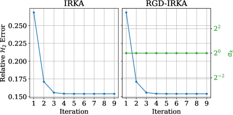
Figure 4: IRKA and RGD-IRKA results for the [GAB08] example, $r=2$, and initial Cauchy index of $0$

Next for $r=2$, we change the initialization to

$$\widehat{E}_{1}=I_{2},\ \widehat{A}_{1}=\begin{bmatrix}-1&0\\ 0&-2\end{bmatrix}\!,\ \widehat{B}_{1}=\mathds{1}_{2\times 1},\ \widehat{C}_{1}=\mathds{1}_{1\times 2},$$

which has Cauchy index of $2$. The results are shown in Figure 5. It shows that, in the SISO case, where the manifold $\Sigma_{r,m,p}^{-}(\mathbb{R})$ is disconnected and RGD-IRKA enforces the iterates to stay on the same connected component, a bad choice of the initial Cauchy index can lead to a bad ROM for RGD-IRKA, but IRKA still converges to a good local minimum since it jumps to a model with a different Cauchy index. Furthermore, we note that the pole-residue form of the ROM from RGD-IRKA is

$$\frac{0.97188}{s+0.27344}+\frac{8.4933}{s+6.9933\times 10^{12}}.$$

It suggests that, since RGD-IRKA is restricted to one connected component due to line search, the iterates converge to the boundary of the connected component, which are systems of lower order. We emphasize that Cauchy index initialization is only a potential concern in the SISO case.

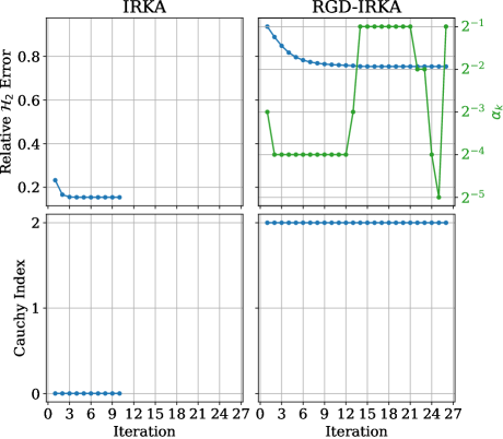
Figure 5: IRKA and RGD-IRKA results for the [GAB08] example, $r=2$, and initial Cauchy index of $2$

9.2 Example 2

Here we show results on the CD player example from the NICONET benchmark collection [CVD02], which is mimo MIMO system with $2$ inputs and $2$ outputs. Figure 6 shows the result for $r=6$, initialized with

$$\widehat{E}_{1}=I_{6},\ \widehat{A}_{1} =\operatorname{\mathsf{diag}}\lparen-1,-2,\dots,-6\rparen,\ \widehat{B}_{1}=\mathds{1}_{6\times 2},$$

$$\widehat{C}_{1} =\mathds{1}_{2\times 6}.$$

Note that, since the manifold $\Sigma_{r,m,p}^{-}(\mathbb{R})$ is now connected, Cauchy index is not necessary (and is not even defined). Here we observe convergence of IRKA with most iterates being unstable. On the other hand, RGD-IRKA converges faster and reaches a slightly better ROM (relative $\mathcal{H}_{2}$ errors are $1.90026\times 10^{-3}$ for IRKA and $1.11674\times 10^{-3}$ for RGD-IRKA).

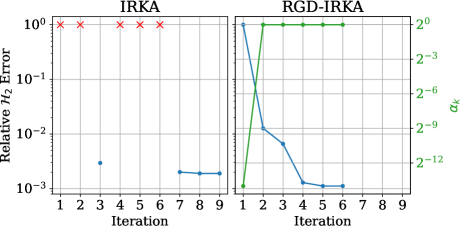
Figure 6: IRKA and RGD-IRKA results for the CD player example and $r=6$. Red crosses represent unstable models

10 Conclusion

We showed that IRKA can be interpreted as a Riemannian gradient descent method with a fixed step size. This interpretation directly leads to a development of a Riemannian gradient descent formulation of IRKA, called RGD-IRKA, that employs variable step size and line search, with guaranteed convergence and stability preservation. Numerical examples illustrated the benefits of RGD-IRKA.

With the Riemannian framework established for IRKA, applying other Riemannian optimization methods in this setting will be an interesting direction for future work. Understanding the RGD-IRKA formulation for structured dynamical systems will be another interesting topic to pursue.

References

• [ABG94] D. Alpay, L. Baratchart, and A. Gombani. On the differential structure of matrix-valued rational inner functions. In A. Feintuch and I. Gohberg, editors, Nonselfadjoint Operators and Related Topics, pages 30–66, Basel, 1994. Birkhäuser Basel. doi:10.1007/978-3-0348-8522-5_2.
• [ABG10] A. C. Antoulas, C. A. Beattie, and S. Gugercin. Interpolatory model reduction of large-scale dynamical systems. In J. Mohammadpour and K. M. Grigoriadis, editors, Efficient Modeling and Control of Large-Scale Systems, pages 3–58. Springer US, Boston, MA, 2010. doi:10.1007/978-1-4419-5757-3_1.
• [ABG20] A. C. Antoulas, C. A. Beattie, and S. Güğercin. Interpolatory methods for model reduction. Computational Science and Engineering 21. SIAM, Philadelphia, PA, 2020. doi:10.1137/1.9781611976083.
• [AM12] P.-A. Absil and J. Malick. Projection-like retractions on matrix manifolds. SIAM J. Optim., 22(1):135–158, 2012. doi:10.1137/100802529.
• [AMS08] P.-A. Absil, R. Mahony, and R. Sepulchre. Optimization Algorithms on Matrix Manifolds. Princeton University Press, Princeton, N.J. Woodstock, 2008. URL: https://press.princeton.edu/absil.
• [BD82] C. I. Byrnes and T. E. Duncan. On certain topological invariants arising in system theory. In New Directions in Applied Mathematics, pages 29–71. Springer New York, 1982. doi:10.1007/978-1-4612-5651-9_3.
• [Bou23] N. Boumal. An introduction to optimization on smooth manifolds. Cambridge University Press, Cambridge, England, March 2023.
• [Bro76] R. Brockett. Some geometric questions in the theory of linear systems. IEEE Trans. Autom. Control, 21(4):449–455, 1976. doi:10.1109/TAC.1976.1101301.
• [Cla66] J. M. C. Clark. The consistent selection of local coordinates in linear system identification. In Joint Automatic Control Conf., pages 576–580, 1966.
• [CVD02] Y. Chahlaoui and P. Van Dooren. A collection of benchmark examples for model reduction of linear time invariant dynamical systems. Technical Report 2002-2, SLICOT Working Note, 2002. Available from www.slicot.org.
• [Del85] D. F. Delchamps. Global structure of families of multivariable linear systems with an application to identification. Mathematical Systems Theory, 18(1):329–380, December 1985. doi:10.1007/bf01699476.
• [GAB06] S. Gugercin, A. C. Antoulas, and C. A. Beattie. A rational Krylov iteration for optimal $\mathcal{H}_{2}$ model reduction. In Proc. of the 17th International Symposium on Mathematical Theory of Networks and Systems, pages 1665–1667, 2006.
• [GAB08] S. Gugercin, A. C. Antoulas, and C. Beattie. $\mathcal{H}_{2}$ model reduction for large-scale linear dynamical systems. SIAM J. Matrix Anal. Appl., 30(2):609–638, 2008. doi:10.1137/060666123.
• [Haz77] M. Hazewinkel. Moduli and canonical forms for linear dynamical systems II: The topological case. Mathematical Systems Theory, 10(1):363–385, December 1977. doi:10.1007/bf01683285.
• [HK76] M. Hazewinkel and R. E. Kalman. On invariants, canonical forms and moduli for linear, constant, finite dimensional, dynamical systems. In G. Marchesini and S. K. Mitter, editors, Mathematical Systems Theory, pages 48–60, Berlin, Heidelberg, 1976. Springer Berlin Heidelberg. doi:10.1007/978-3-642-48895-5_4.
• [JW19] Y. Jiang and W. Wang. $H_{2}$ optimal model order reduction of the discrete system on the product manifold. Applied Mathematical Modelling, 69:593–603, 2019. doi:10.1016/j.apm.2019.01.012.
• [JX19] Y. Jiang and K. Xu. Model order reduction of port-Hamiltonian systems by Riemannian modified Fletcher–Reeves scheme. IEEE Transactions on Circuits and Systems II: Express Briefs, 66(11):1825–1829, 2019. doi:10.1109/TCSII.2019.2895872.
• [JX20] Y. Jiang and K. Xu. Riemannian modified Polak-Ribière-Polyak conjugate gradient order reduced model by tensor techniques. SIAM J. Matrix Anal. Appl., 41(2):432–463, 2020. doi:10.1137/19M1257147.
• [JX21] Y. Jiang and K. Xu. Frequency-limited reduced models for linear and bilinear systems on the Riemannian manifold. IEEE Trans. Autom. Control, 66(9):3938–3951, 2021. doi:10.1109/TAC.2020.3027643.
• [Kli11] W. P. A. Klingenberg. Riemannian Geometry. De Gruyter, 2011. doi:10.1515/9783110905120.
• [Lan95] S. Lang, editor. Differential and Riemannian Manifolds. Springer New York, 1995. doi:10.1007/978-1-4612-4182-9.
• [Lee12] J. M. Lee. Introduction to Smooth Manifolds. Springer New York, 2012. doi:10.1007/978-1-4419-9982-5.
• [LJX22] Z. Li, Y. Jiang, and K. Xu. Riemannian optimization model order reduction method for general linear port-Hamiltonian systems. IMA Journal of Mathematical Control and Information, 39(2):590–608, March 2022. doi:10.1093/imamci/dnac001.
• [ML66] L. Meier and D. G. Luenberger. Approximation of linear constant systems. In Joint Automatic Control Conf., pages 585–588, 1966.
• [ML67] L. Meier and D. G. Luenberger. Approximation of linear constant systems. IEEE Trans. Autom. Control, 12(5):585–588, 1967. doi:10.1109/TAC.1967.1098680.
• [Mli23] P. Mlinarić. Riemannian gradient descent IRKA experiments, November 2023. URL: https://github.com/pmli/rgd-irka-experiments/tree/v1.
• [MRS16] R. Milk, S. Rave, and F. Schindler. pyMOR – generic algorithms and interfaces for model order reduction. SIAM J. Sci. Comput., 38(5):S194–S216, 2016. doi:10.1137/15M1026614.
• [NAP08] Yasunori Nishimori, Shotaro Akaho, and Mark D. Plumbley. Natural conjugate gradient on complex flag manifolds for complex independent subspace analysis. In Artificial Neural Networks - ICANN 2008, pages 165–174. Springer Berlin Heidelberg, 2008. doi:10.1007/978-3-540-87536-9_18.
• [Sat17a] K. Sato. Riemannian optimal control and model matching of linear port-Hamiltonian systems. IEEE Trans. Autom. Control, 62(12):6575–6581, 2017. doi:10.1109/TAC.2017.2712905.
• [Sat17b] K. Sato. Riemannian optimal model reduction of linear second-order systems. IEEE Contr. Syst. Lett., 1(1):2–7, 2017. doi:10.1109/LCSYS.2017.2698178.
• [Sat18] K. Sato. Riemannian optimal model reduction of linear port-Hamiltonian systems. Automatica, 93:428–434, 2018. doi:10.1016/j.automatica.2018.03.051.
• [Sat19] K. Sato. Riemannian optimal model reduction of stable linear systems. IEEE Access, 7:14689–14698, 2019. doi:10.1109/ACCESS.2019.2892071.
• [SS15] H. Sato and K. Sato. Riemannian trust-region methods for $H^{2}$ optimal model reduction. In 54th IEEE Conference on Decision and Control (CDC), pages 4648–4655, 2015. doi:10.1109/CDC.2015.7402944.
• [SS16] H. Sato and K. Sato. A new $H^{2}$ optimal model reduction method based on Riemannian conjugate gradient method. In 55th IEEE Conference on Decision and Control (CDC), pages 5762–5768, 2016. doi:10.1109/CDC.2016.7799155.
• [SS18] K. Sato and H. Sato. Structure-preserving $H^{2}$ optimal model reduction based on the Riemannian trust-region method. IEEE Trans. Autom. Control, 63(2):505–512, 2018. doi:10.1109/TAC.2017.2723259.
• [WJ18] W. Wang and Y. Jiang. $H_{2}$ optimal model order reduction on the Stiefel manifold for the MIMO discrete system by the cross Gramian. Mathematical and Computer Modelling of Dynamical Systems, 24(6):610–625, 2018. doi:10.1080/13873954.2018.1519835.
• [WJ22] W. Wang and Y. Jiang. HSH-norm optimal MOR for the MIMO linear time-invariant systems on the Stiefel manifold. International Journal of Control, 95(12):3274–3282, 2022. doi:10.1080/00207179.2021.1971299.
• [XJ19] Kang-Li Xu and Yao-Lin Jiang. An unconstrained $H_{2}$ model order reduction optimisation algorithm based on the Stiefel manifold for bilinear systems. International Journal of Control, 92(4):950–959, 2019. doi:10.1080/00207179.2017.1376115.
• [XJ22] K. Xu and Y. Jiang. Riemannian optimization approach to structure-preserving model order reduction of integral-differential systems on the product of two Stiefel manifolds. Journal of the Franklin Institute, 359(9):4307–4330, 2022. doi:10.1016/j.jfranklin.2022.04.012.
• [XJY15] K. Xu, Y. Jiang, and Z. Yang. $H_{2}$ order-reduction for bilinear systems based on Grassmann manifold. Journal of the Franklin Institute, 352(10):4467–4479, 2015. doi:10.1016/j.jfranklin.2015.06.022.
• [XJY17] K. Xu, Y. Jiang, and Z. Yang. $H_{2}$ optimal model order reduction by two-sided technique on Grassmann manifold via the cross-gramian of bilinear systems. International Journal of Control, 90(3):616–626, 2017. doi:10.1080/00207179.2016.1186845.
• [XZ13] Y. Xu and T. Zeng. Fast optimal $\mathcal{H}_{2}$ model reduction algorithms based on Grassmann manifold optimization. Int. J. Numer. Anal. Model., 10(4):972–991, 2013. URL: http://www.math.ualberta.ca/ijnam/Volume-10-2013/No-4-13/2013-04-13.pdf.
• [YJ17] P. Yang and Y. Jiang. $H_{2}$ optimal model reduction of coupled systems on the Grassmann manifold. Mathematical Modelling and Analysis, 22(6):785–808, November 2017. doi:10.3846/13926292.2017.1381863.
• [YJX19] P. Yang, Y. Jiang, and K. Xu. A trust-region method for $H_{2}$ model reduction of bilinear systems on the Stiefel manifold. Journal of the Franklin Institute, 356(4):2258–2273, 2019. doi:10.1016/j.jfranklin.2019.01.024.
• [YL99] W.-Y. Yan and J. Lam. An approximate approach to $\mathcal{H}_{2}$ optimal model reduction. IEEE Trans. Autom. Control, 44(7):1341–1358, 1999. doi:10.1109/9.774107.