Gravitational waves radiated from axion string-wall networks

Abstract

We examine gravitational waves (GWs) emitted from axionic strings and domain walls (DWs) in the early universe using advanced 3D lattice simulations. Our study encompasses scenarios for domain wall numbers $N_{\rm DW}=1$ and $N_{\rm DW}>1$, which correspond to GWs primarily from strings and DWs, respectively. Simulations begin before the Peccei-Quinn (PQ) phase transition and conclude with the destruction of string-wall networks below the QCD energy scale, relevant to both QCD axions and axion-like particles (ALPs). For $N_{\rm DW}=1$, the GW energy density from axion strings appears undetectable for both QCD axions and ALPs. In contrast, for $N_{\rm DW}>1$, the GW spectrum is largely determined by the bias term’s coefficient, with the QCD axion model predicting undetectable GW emissions, while the ALPs model allows for a detectable GW signal in the nano-Hertz to the kilo-Hertz frequency range.

Introduction. Axions are ultralight pseudo-scalar particles realized by the PQ mechanism originally introduced to resolve the Strong CP problem in quantum chromodynamics (QCD) Peccei and Quinn (1977a, b); Wilczek (1978). Afterward, the QCD axion and more generally the axion-like particles (ALPs), as dark matter (DM) candidates gave rise to widespread interest Weinberg (1978); Abbott and Sikivie (1983); Dine and Fischler (1983); Preskill et al. (1983). Moreover, the post-inflationary PQ symmetry breaking scenario with accompanying axion topological defects, the axion string and DWs, that will radiate axion particles Kawasaki et al. (2015) and have impact on the form of axion relic abundance as well as the cosmic structure formation Hogan and Rees (1988); Kolb and Tkachev (1993, 1994a, 1994b); Zurek et al. (2007); Enander et al. (2017); Vaquero et al. (2019); Buschmann et al. (2020); Chang and Cui (2023). The thorough studies on those subjects may provide viable search avenues for axion models Marsh (2016); Borsanyi et al. (2016); Hlozek et al. (2015); Kawasaki and Nakayama (2013); Chang and Cui (2020, 2022); Auclair et al. (2023a); Brzeminski et al. (2022); Agrawal et al. (2022); Jain et al. (2021, 2022); Agrawal et al. (2020); Dessert et al. (2022), given that the direct experimental detection Shokair et al. (2014); Du et al. (2018); Brubaker et al. (2017a); Al Kenany et al. (2017); Brubaker et al. (2017b); Caldwell et al. (2017); Kahn et al. (2016); Ouellet et al. (2019a, b); Chaudhuri et al. (2015); Silva-Feaver et al. (2017) based on the axion particle per se is extremely difficult.

Besides, axion strings and DWs are known to be the stochastic gravitational wave backgrounds (SGWBs) sources that are important scientific goals of many GW detection experiments, such as pulsar timing array (PTA)Blasi et al. (2021); Samanta and Datta (2021); Ellis and Lewicki (2021); Bian et al. (2022a); Afzal et al. (2023); Bian et al. (2021, 2023, 2022b); Ferreira et al. (2023), LISAAuclair et al. (2023b); Boileau et al. (2022), and LIGO Abbott et al. (2021). After the spontaneous breaking of the $U(1)_{PQ}$ symmetry occurs at $T\sim f_{a}$ (with $f_{a}$ the axion decay constant), axion string forms and eventually evolves into the scaling regime Kibble (1976); Shellard and Battye (1998); Sikivie (2008); Kim and Carosi (2010); Yamaguchi et al. (1999); Yamaguchi and Yokoyama (2003); Hiramatsu et al. (2011a), and is expected to generate an SGWB with a very wide and nearly scale-invariant GW spectrum Gouttenoire et al. (2020); Auclair et al. (2020). As the universe cools, the $U(1)$ symmetry will be explicitly broken at a lower scale $\Lambda$ (e.g. $\Lambda_{\rm QCD}$ for QCD axion), and axion acquires a mass $m\sim\Lambda^{2}/f_{a}$ through non-perturbative effects Dine et al. (1981); Zhitnitsky (1980); Kim (1987). Meanwhile, DWs bounded by strings are formed. The fate of the string-wall system depends on the specific axion model and is characterized by the DW number $N_{\rm DW}$. In the KSVZ model Kim (1979); Shifman et al. (1980) with $N_{\rm DW}=1$, only one domain wall is attached to each string. The DWs are short-lived and quickly annihilate when $H(T_{\rm dec})\simeq m$ due to the tension of walls, thus strings will dominate the dynamics and SGWB of the system. In the $N_{\rm DW}>1$ case obtained by DFSZ model Dine et al. (1981); Zhitnitsky (1980), $N_{\rm DW}$ walls attached to a string, balance the tension among themselves and lead to stable DWs. However, the stable DWs would eventually dominate the universe and therefore conflict with cosmological observations Sikivie (1982); Zeldovich et al. (1974). The conventional way to solve this DW problem is to introduce a bias term Gelmini et al. (1989); Larsson et al. (1997) to explicitly break the $Z_{N_{\rm DW}}$ discrete symmetry so that the walls will annihilate under the pressure differences between different vacua before they overclose the universe. The bias term may originate from the fundamental physics at Planck scale Kamionkowski and March-Russell (1992); Holman et al. (1992); Dobrescu (1997); Barr and Seckel (1992); Dine (1992), and should lead to long-lived DWs due to limitations from the degree of CP violation Barr and Seckel (1992). The long-lived DWs will generate an SGWB that is much stronger than that of short-lived DWs, which may have sufficient observable amplitudes Hiramatsu et al. (2011b); Liu et al. (2021).

The previous simulations for pure global (axion) strings imply that the relevant SGWB would not be strong enough to be detected Figueroa et al. (2013). This can be explained by the GW emission being highly suppressed compared to particle radiation for global strings Baeza-Ballesteros et al. (2023); Saurabh et al. (2020). On the other hand, there are several semi-analytical and numerical studies on axion string-wall hybrid networks with $N_{\rm DW}=1$ or $N_{\rm DW}>1$. In the case of $N_{\rm DW}>1$, the early 2D lattice simulations Hiramatsu et al. (2011b) investigated the dynamics of the string-wall system including the bias term, where the corresponding GW spectrum is not measured. The later studiesHiramatsu et al. (2013) performed 3D lattice simulations to measure the spectra of axion and GWs radiated by long-lived DWs, however, the bias term is not included. In this Letter, we focus on the SGWB that is produced by axion-associated topological defects. We aim to conduct a relatively complete and realistic numerical study on the SGWB radiated by string-wall networks. We perform high-resolution 3D lattice simulations with $2200^{3}$ grid-sites for both the $N_{\rm DW}=1$ case and the $N_{\rm DW}>1$ case with different coefficient of bias term, and measure the GW spectrum. Our simulation begins before the PQ phase transition and ends at the annihilation of the string-wall network below the QCD confinement scale. Our studies show that it’s possible to probe or exclude axion models with current and forthcoming GW detectors, e.g. determine or constrain the model parameters such as $f_{a}$ and $m$, this will also be helpful for direct experimental searches on axion particles.

The simulation framework. Consider the Lagrangian of the PQ complex scalar field $\varphi$, given by

with $\lambda$ the PQ coupling constant, $v$ the PQ vacuum, $T$ the temperature, $m(T)$ the temperature-dependent QCD axion mass, $\theta={\rm Arg}(\varphi)$ the dimensionless axion field, $\Xi$ the coefficient of bias term. For the bias term, $\delta$ only determines the location of the true minimum of the potential in numerical simulations, so we can fix $\delta=0$ for all of our simulations, this will not affect the quantitative results Hiramatsu et al. (2011b). When $T>100$ ${\rm MeV}$, $m(T)$ can be parametrized as Wantz and Shellard (2010)

$$m(T)^{2}=\frac{\alpha_{a}\Lambda^{4}}{f_{a}^{2}(T/\Lambda)^{6.68}},$$ (1)

where $\alpha_{a}=1.68\times 10^{-7}$, $\Lambda=400\,\mathrm{MeV}$ and $f_{a}=v/N_{\rm DW}$. When $T\leq 100$ ${\rm MeV}$, the axion mass no longer grows and is substituted by a zero-temperature mass $m_{0}=5.707\times 10^{-5}(10^{11}\,\,{\rm GeV}/f_{a})$ eV Grilli di Cortona et al. (2016). Without loss of universality, we take the QCD axion scenario as a benchmark to perform simulations, and with our careful simulation setup, the numerical results can be applied to the ALPs with constant mass $m=m_{0}$ and the same axion decay constant $f_{a}$.

Our simulation is divided into two stages, namely the PQ era and the QCD era, which correspond to the spontaneous breaking of PQ symmetry near the scale of $T\sim v$ Kim (1979); Shifman et al. (1980); Dine et al. (1981); Zhitnitsky (1980); Srednicki (1985) and the explicit breaking near the QCD scale, respectively. In the PQ era, the second line in Eq. (LABEL:full_lagrangian) caused by QCD effects can be neglected. The critical temperature at which the system undergoes a second-order phase transition is $T_{\rm c}=\sqrt{3}v$. Our simulation begins at an initial temperature $T_{i}=2.4T_{\rm c}$, and we set $v=2\times 10^{17}$ ${\rm GeV}$ to ensure the simulation box can capture enough Hubble volumes. The initial configuration of $\varphi$ can be obtained by thermal spectrum. The fields are rescaled with the PQ vacuum $v$, while the comoving lattice spacing $\delta x$ (and time-step) are rescaled by $w_{*}=a_{i}H_{i}$ with the $a_{i}$ and $H_{i}$ being initial scale factor and Hubble parameter. For convenience, we use the rescaled conformal time $\tilde{\eta}$ $(=\eta/\eta_{i})$ with the initial conformal time being $\eta_{i}=1/(a_{i}H_{i})$ in our simulations. We fix $\tilde{\eta}=1$ to be the initial time at which $T=T_{i}$, so the PQ phase transition happens at $\tilde{\eta}=T_{\rm i}/T_{c}=2.4$. We set $\lambda=0.2$ here for concreteness.

The comoving side length of the simulation box and the number of grid points per side are set to $L_{\rm PQ}=1680/(a_{i}H_{i})$ and $N=2200$, respectively. So, the dimensionless comoving lattice spacing is about $\delta\tilde{x}=0.764$, and the time-step is chosen as $\delta\tilde{\eta}=0.02$. We use the second-order leap-frog algorithm adopted by ${\mathcal{C}osmoLattice}$ Figueroa et al. (2023, 2021) to evolve the equations of motion. After the PQ phase transition, the axion string network forms and evolves towards a scaling regime. We continue to evolve the string network until the final moment $\tilde{\eta}_{f}=105$ (for the convenience of calculating scaling parameter near $\tilde{\eta}_{f}=105$, we evolve the string network to $\tilde{\eta}=121$), see FIG. 1. At $\tilde{\eta}_{f}=105$, the simulation box contains $16^{3}$ Hubble volumes, and the string core width is 4.1 times the physical lattice spacing due to we have used the fat string algorithm to adjust $\lambda$ Moore et al. (2002).

For simulations in the QCD era, it can be extrapolated that the scaling regime of axion string networks in the PQ era has been maintained until the QCD energy scale Hindmarsh et al. (2020). Therefore, we take the field configurations at the final moment of PQ era as the initial configurations, while keeping the same number of Hubble volumes in the simulation box. In this way, we maintain the correct number density of axion strings per Hubble volume and the status of modes relative to the horizon.

Our simulation in the QCD era starts before the QCD phase transition, with an initial temperature $T_{1}=220$ ${\rm MeV}$. We reinterpret the comoving side length of the simulation box as $L_{\rm QCD}=16/(a_{1}H_{1})$, with $a_{1}$ ($H_{1}$) the initial scale factor (Hubble parameter). Therefore, the simulation box contains $16^{3}$ Hubble volumes identical to that at the final moment of the PQ era. Due to the scaling property of the axion string network, different PQ symmetry-breaking scales will finally lead to the same dimensionless field configurations after the string networks enter the scaling regime. So we can reinterpret the PQ vacuum as $v_{\rm re}=N_{\rm DW}\cdot f_{a}$ for different $N_{\rm DW}$, with fixed decay constant $f_{a}=1.8\times 10^{16}$ ${\rm GeV}$. Although there exist the astrophysical and cosmological bound for $f_{a}$ in the QCD axion scenario Raffelt (1990, 2008); Hiramatsu et al. (2011a), $4\times 10^{8}~{}{\rm GeV}<f_{a}<3\times 10^{11}~{}{\rm GeV}$, we set $f_{a}$ high enough in simulation to ensure that the DW forms shortly before the QCD phase transition. Thus, our simulation will encompass both the QCD phase transition and the state where the axion achieves zero temperature mass for a long time. Given that the coefficient of the bias term is a constant in a single simulation, the axion needs to reach zero temperature mass (constant mass) as soon as possible, this will help us to apply the simulation results to ALPs with constant mass.

We use the rescaled conformal time $\hat{\eta}$ $(=\eta/\eta_{1}=a/a_{1})$ to perform time iteration, with the initial conformal time $\eta_{1}=1/(a_{1}H_{1})$. Furthermore, we take into account the changes in the number of relativistic degrees of freedom near the QCD scale Wantz and Shellard (2010), which will affect the evolution of the scale factor and the measurement of the GW spectrum. The fields are rescaled with the reinterpreted PQ vacuum $v_{\rm re}$, and the comoving lattice spacing (and time-step) are rescaled with $\hat{w}=6a_{1}H_{1}$. So, the dimensionless comoving lattice spacing is $\delta\hat{x}\approx 0.0436$, and the time-step is chosen as $\delta\hat{\eta}=0.0064$.

To resolve the resolution of string throughout our simulation, we adjust the string width by defining the parameter $\tilde{\lambda}\equiv\lambda v_{\rm re}^{2}/m(\hat{\eta}_{\rm e})^{2}$, where $\hat{\eta}_{\rm e}\approx 1.16$ is the time at which $m=H$ is satisfied Buschmann et al. (2020). At the initial time, we set $\tilde{\lambda}=1900$ so that the string width is about 4.1 times the physical lattice spacing, $\delta_{\rm st}/\delta x_{\rm phy}$=4.1, which is equal to the ratio of the two at the final time of the PQ era. As the physical lattice spacing increases, when $\delta_{\rm st}/\delta x_{\rm phy}=1.5$ is satisfied, we use the fat string algorithm to adjust $\tilde{\lambda}$ to keep this ratio always hold for the rest time. After $\hat{\eta}\simeq 2.9$, the relation $\sigma_{\rm wall}>\mu_{\rm string}(t)/t$ is satisfied, with $\sigma_{\rm wall}\sim 8mf_{a}^{2}$ the DW tension, $\mu_{\rm string}(t)=\pi v_{\rm re}^{2}{\rm ln}(t/\delta_{\rm s})$ the mass energy density of string, and $\delta_{\rm st}\simeq 1/(\sqrt{\tilde{\lambda}}m(\hat{\eta}_{\rm e}))$ the string width, the dynamics and SGWB will dominated by the tension of DWs. Therefore, the artificial breaking of the ratio of string width to physical lattice spacing will not have a significant impact on the final simulation results.

When $m(\hat{\eta})=3H(\hat{\eta})$ is satisfied at $\hat{\eta}\approx 1.58$, axion begins to feel the pull of its mass, and DWs bounded by strings are formed. Afterward, as the temperature decreases to $100$ MeV at $\hat{\eta}\approx 3.32$, the axion mass and the surface mass density of DWs no longer change. We continue to evolve the equations of motion until the final time $\hat{\eta}=21$, at which the temperature is $T_{f}=18.4$ ${\rm MeV}$. At this time, the physical side length of the simulation box is greater than one Hubble length, and the string core width as well as the DW thickness ($\delta_{\rm dw}\sim 1/m_{0}$) are both greater than physical lattice spacing.

Results. In the PQ era, we measured the scaling parameters of the axion string in two ways, see FIG. 1. One is the method explained in Refs. Hiramatsu et al. (2013) ($\xi$, blue hollow points), we call it the traditional method, and the other is the standard scaling model Hindmarsh et al. (2020) based on the mean string separation ($\xi_{\rm s}$, red hollow point). At the final time ($\tilde{\eta}_{f}=105$), the string networks reach scaling regime approximately ($\xi_{\rm s}\approx 0.55$). We found that the scaling parameters exhibited logarithmic increase behavior under two measurement schemes. Several groups have reported logarithmic increase behavior while using the traditional method Gorghetto et al. (2018); Kawasaki et al. (2018); Vaquero et al. (2019); Buschmann et al. (2020). However, according to reference Hindmarsh et al. (2020), there should be no more logarithmic increase after adopting the standard scaling model. We preliminarily deduce that this may be caused by insufficient resolution of the Hubble volume, given that the simulation box contains too much Hubble volume during the PQ phase transition. We have prepared an additional PQ era specifically for measuring GWs radiated by pure global (axion) strings, where the string network stays in the scaling regime for a long time and the scaling parameters do not exhibit a logarithmic increase, see Supplemental Material. A thorough explanation of the logarithmic increase behavior is beyond the scope of this article, we leave this for future study.

Figure 1: Evolution of scaling parameters with rescaled conformal time $\tilde{\eta}$ and rescaled cosmic time $\tilde{t}=t/t_{i}$, with $t_{i}=1/(2H_{i})$ the initial cosmic time. In a radiation-dominated universe, the scaling parameter is equal to four times the number of infinite (long straight) strings per Hubble volume. The red and blue dashed lines represent the logarithmic fit of the scaling parameters in two measurement schemes. The black vertical dashed line represents the time we selected as the final moment of the PQ era.

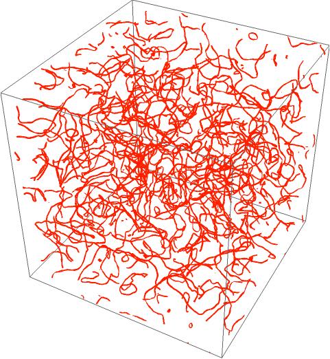
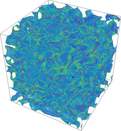
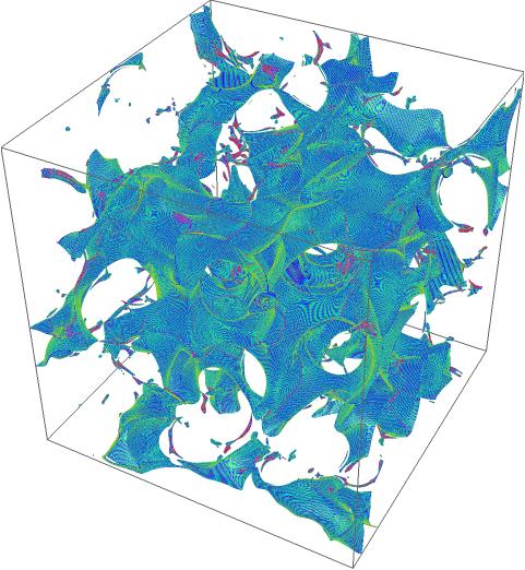
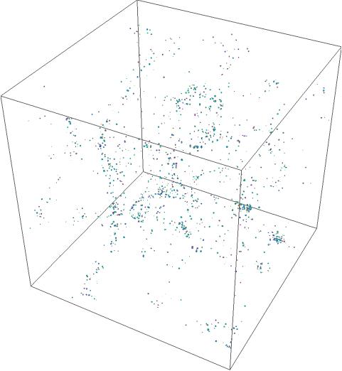
Figure 2: 3D snapshots of the string-wall networks at different times in the $1100^{3}$ sub-lattice, with $N_{\rm DW}=3$ and $\Xi=2.5\times 10^{-72}$. The four plots arranged from top-left to bottom-right were recorded at the time $\hat{\eta}$=1, 2.6, 6.6, and 13. The blue and the red region indicate where the DW and string exists, respectively.

In the QCD era, for simulations in the $N_{\rm DW}>1$ scenario, we fix $N_{\rm DW}=3$ as a benchmark, and choose $\Xi=[0$, $2.5\times 10^{-72}$, $5\times 10^{-72}$, $1.5\times 10^{-71}]$ to investigate the effects of the bias term. Our choice of $\Xi$ is based on two theoretical constraints with model parameters $f_{a}=1.8\times 10^{16}$ GeV and the corresponding zero-temperature axion mass $m=m_{0}$. The first constraint is that the decay of walls is required to occur before wall domination, so there is a lower bound on bias term, $\Xi\geqslant 8.96\times 10^{-37}N_{\rm DW}^{-3}\alpha(m/{\rm GeV})^{2}$, with $\alpha$ a numerical coefficient can be fixed from simulation. The second constraint comes from that we expect the axion mass to be dominated by non-perturbative effects rather than the bias term, $\Xi\leqslant\frac{1}{2}N_{\rm DW}^{-2}f_{a}^{-2}m^{2}$, otherwise, the cosmological history will be significantly modified Hiramatsu et al. (2013). By using the semi-analytical formula obtained from our simulation results (see Eq. (2)), we can reinterpret the model parameters like $N_{\rm DW}$, $f_{a}$, $m$ and $\Xi$ to obtain the correct scenario in the restricted parameter space of QCD axion or ALPs. We recorded the 3D distribution of the string-wall networks at different times (see FIG. 2), where we show that string configurations appear after PQ symmetry breaking (top-left plot), string-wall networks form after $m=3H$ (top-right plot) and decay latter (bottom two plots) as the Universe cools down. We find that the decay rate of the DW is proportional to $\Xi$ through the calculation of the comoving area density defined in the Supplemental Material.

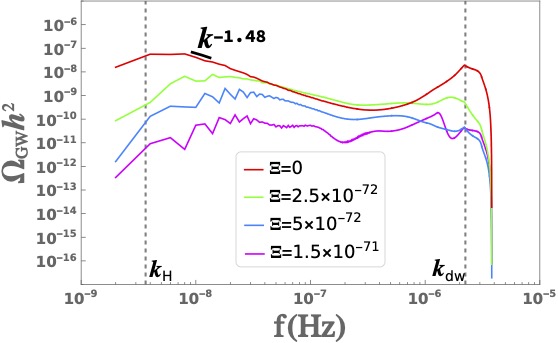
Figure 3: The GW power specra today for different values of $\Xi$ in the case of $N_{\rm DW}=3$. The two black dashed lines denote the dimensionless comoving momentum corresponding to the Hubble radius and the thickness of DW at $T_{\rm dec}$ in the case of $\Xi=2.5\times 10^{-72}$.

We then study the GW spectrum for the string-wall networks. Theoretically, when the DW dominates the GWs radiated from string-wall networks, the energy density of GWs today can be estimated by using the quadrupole formula Poisson (2008); Hiramatsu et al. (2013)

$$\frac{\rho_{\rm gw}(t_{0})}{\rho_{c}(t_{0})/h^{2}}=7.04\times 10^{-74}g_{*}(T_{\rm dec})^{-\frac{1}{3}}\epsilon_{\rm gw}\mathcal{A}^{2}N_{\rm DW}^{-6}\frac{\alpha^{2}m^{4}}{\Xi^{2}{\rm GeV}^{4}},$$ (2)

where $\epsilon_{gw}\approx 5$ and $\mathcal{A}\approx 1$ are GW efficiency parameter and area parameter of DWs in the case of $N_{\rm DW}=3$, and would be different for other $N_{\rm DW}$ Hiramatsu et al. (2013). The collapse of the DW occurs at the temperature when the pressure induced by bias term overcomes the DW tension, which can be estimated by $T_{\rm dec}=1.92\times 10^{9}\times g_{*}({T_{\rm dec}})^{-1/4}f_{a}N_{\rm DW}^{3/2}(\alpha m/{\rm GeV})^{-1/2}\Xi^{1/2}$, which close to the temperature when the value of comoving area density becomes 1% of that with $\Xi=0$ Hiramatsu et al. (2011b). We measure the GW spectra for different bias term to numerically check the justification of Eq. 2. As theoretically expected, the ratio of the energy density is found to be: $\rho_{\rm gw}(\Xi_{1})/\rho_{\rm gw}(\Xi_{2})\simeq(\Xi_{2}/\Xi_{1})^{2}=4,~{}\rho_{\rm gw}(\Xi_{2})/\rho_{\rm gw}(\Xi_{3})\simeq(\Xi_{3}/\Xi_{2})^{2}=9$, with $(\Xi_{1},\Xi_{2},\Xi_{3})=(2.5,5,15)\times 10^{-72}$. The numerical coefficient is determine to be $\alpha=22.1$ through our simulations for the three different bias terms. The GW spectra produced by string-wall networks at different $\Xi$ are shown in FIG. 3. For $\Xi>0$, the GW spectrum will have peaks at two characteristic scales $k_{\rm H}$ and $k_{\rm dw}$, corresponding to the Hubble radius and the thickness of the DW ($\delta_{\rm dw}$) at the decay temperature of DWs, with $k_{\rm H}=2\pi H(T_{\rm dec})\times a(T_{\rm dec})/(a_{1}H_{1})$ and $k_{\rm dw}=2\pi/\delta_{\rm dw}\times a(T_{\rm dec})/(a_{1}H_{1})$, see FIG. 3. The peak frequency corresponding to the Hubble radius at $T_{\rm dec}$ is $f_{\rm peak}=7.32\times 10^{-8}\times g_{*}(T_{\rm dec})^{1/6}(T_{\rm dec}/{\rm GeV})$ Hz. We find that the proportional relationship for the GWs energy density still holds for the peak amplitude (left peak) of the GW spectrum. Similarly, for the peak amplitude of GW spectrum $(\Omega_{\rm GW}h^{2})_{\rm peak}$, we directly substitute $\alpha$ with $\alpha_{\rm peak}=0.147$ in Eq. (2). In the case of $\Xi=0$, the GW spectrum decreases as  $k^{-1.48}$ near the left peak, different from the slope of $k^{-1}$ for DWs in previous simulations Saikawa (2017). Note that the right peaks of the four curves are relatively high, which may be due to the insufficient time for the DW to radiate GWs, resulting in the left peak not being high enough Li et al. (2023).

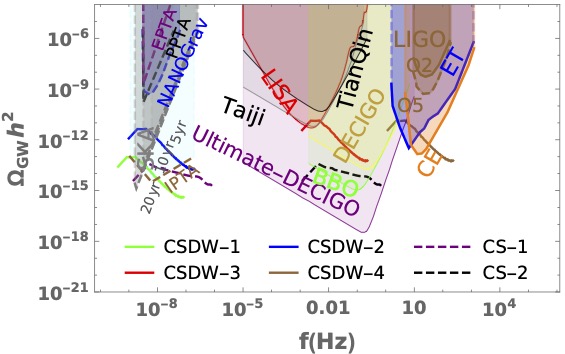
Figure 4: GWs spectra to be probed at present for ALPs. The four solid lines CSDW-1,2,3,4 represent peak amplitude of GWs produced by string-wall networks corresponds to the model parameters ($f_{a}/{\rm GeV}$, $m/{\rm GeV}$, $\Xi$) = ($5\times 10^{10}$, $10^{-11}$, $7\times 10^{-55}$), ($10^{6}$, $1$, $10^{-33}$), ($10^{11}$, $5\times 10^{2}$, $10^{-28}$), ($10^{13}$, $5\times 10^{4}$, $10^{-24}$) in the case of $N_{\rm DW}=3$. The two dashed lines CS-1,2 represent the GW spectrum radiated by pure cosmic (axion) strings corresponding to unrestricted model parameters ($f_{a}/{\rm GeV}$, $m/{\rm GeV}$) = ($6\times 10^{15}$,$10^{-21}$), ($6\times 10^{15}$,$10^{-9}$) in the case of $N_{\rm DW}=1$.

We first note that, for the QCD axion, the constraint from the experimental nEDM (neutron electric dipole moment) bound also sets the upper bound on the bias term which is connected with the strong CP-violation. And, that the axion abundance should not exceed the observed value of the abundance of cold dark matter (CDM) $\Omega_{\rm CDM}h^{2}=0.11$ leads to an upper bound on $f_{a}$ and a more stringent lower bound on $\Xi$ Hiramatsu et al. (2013). With these theoretical constraints together with constraints on dark radiation from axion Chang and Cui (2022); Gorghetto et al. (2021) and other existing experiment constraints O’Hare (2020), we found that the peak amplitude of GWs radiated by the string-wall network is too weak, and will not exceed $(\Omega_{\rm GW}h^{2})_{\rm peak}\lesssim 1.9\times 10^{-35}$ in the whole viable parameter region (the maximum is taken at $f_{a}=4\times 10^{8}$ GeV, $m=1.43\times 10^{-11}$ GeV, $\Xi=7.17\times{10^{-44}}$ for $N_{\rm DW}=3$).

For ALPs, they can greatly alleviate the limitation that comes from CDM abundance by behaving as dark radiation or decaying into Standard Model particles. We can also ignore the nEDM bound, given that ALPs can be unrelated to the strong CP problem in QCD. For this scenario, we found that there is a large range of parameter spaces that can lead to detectable GW signals radiated from string-wall networks. Based on Eq. 2 (replace $\alpha$ with $\alpha_{\rm peak}=0.147$), we present the detectability of SGWB from axion string-wall networks with various model parameters in FIG. 4, see the four benchmark scenarios of CSDW-$1,2,3,4$ (we fix $N_{\rm DW}=3$). We use the shape near the left peak in the case of $\Xi=0$ in FIG. 3 to draw the four curves of string-wall GW spectra, given that this is close to the shape of GW spectrum when $\Xi$ is relatively small.

For the $N_{\rm DW}=1$ scenario with the reinterpreted PQ vacuum $v_{\rm re}=1.8\times 10^{16}$ GeV. We numerically confirmed that the ratio of GWs radiated by string-walls to the GWs radiated by pure strings (with PQ vacuum $v=v_{\rm add}$), satisfies $\Omega_{\rm GW}(v=v_{\rm re})/\Omega_{\rm GW}(v=v_{\rm add})\approx(v_{\rm re}/v_{\rm add})^{4}$, consistent with the analytical calculation of GW spectrum for global strings: $\Omega_{\rm GW}h^{2}\propto(v/M_{\rm pl})^{4}$ Figueroa et al. (2013), see Supplemental Material. Therefore, it can be inferred that GWs are dominated by strings as generally expected. According to the GW spectrum of pure strings obtained from our simulation with peak amplitude $(\Omega_{\rm GW}h^{2})_{\rm peak}=3.41\times 10^{-10}$ and PQ vacuum $v_{\rm add}=6\times 10^{16}$ GeV, if we require the peak amplitude of GWs today satisfies $(\Omega_{\rm GW}h^{2})_{\rm peak}>10^{-15}$, then $v>2.41\times 10^{15}$ GeV is required. But according to the limitations on the $(f_{a},m)$ space of axion O’Hare (2020), the axion mass needs to meet $m\lesssim 10^{-30}$ GeV or $m\gtrsim 4\times 10^{4}$ GeV, corresponding to the GW peak frequency $f\lesssim 1.38\times 10^{-13}$ Hz or $f\gtrsim 2.75\times 10^{4}$ Hz, respectively. Therefore, the GWs radiated by the axion string are too weak to be probed, as shown by the benchmark scenario of CS-1 and CS-2 in FIG. 4.

Conclusion and discussion. The cosmic strings and DWs are generally predicted in many particle physics models beyond the Standard Model, both of them are important SGWB sources. In this Letter, we numerically studied the SGWB produced by string-wall networks in the axion models with different DW numbers and model parameters. Our simulation results apply to both QCD axion and general axion-like particles (ALPs). We found that in the $N_{\rm DW}=1$ case, for both QCD axion and ALPs, the string-dominated SGWB is too weak to be observed. In the $N_{\rm DW}>1$ case, the shape of the GW spectrum will depend on the coefficient of the bias term. For QCD axion, the resulting GWs are also not sufficient to be detected since the parameter space is more tightly restricted. For ALPs, we used the semi-analytic formulas obtained through numerical simulations to determine the peak amplitude and frequency of GWs given by parameter space. We found that ALPs have a considerable $(f_{a},m)$ parameter space that can create detectable GWs from nano-Hertz to kilo-Hertz frequency range. This makes it possible to probe axion models with current and upcoming gravitational wave detectors.

The axion string-wall also radiates free axions when radiating GWs. The resulting axion abundance today can be interpreted as cold dark matter, while the form in which axion abundance exists (e.g. axion minihalos Kolb and Tkachev (1994a); Vaquero et al. (2019); Buschmann et al. (2020)) is not fully understood. Research on this topic can help determine or constrain model parameters, thus forming a complementary and consistent image with the study of GWs, we leave this for later study.

Acknowledgements. We are grateful to Adrien Florio and Daniel G. Figueroa for helpful discussions on their public code ${\mathcal{C}osmoLattice}$. The numerical calculations in this study were carried out on the ORISE Supercomputer. This work is supported by the National Key Research and Development Program of China under Grant No. 2020YFC2201501 and 2021YFC2203004. L.B. is supported by the National Natural Science Foundation of China (NSFC) under Grants Nos. 12075041 and 12147102, 12322505. R.G.C is supported by the National Key Research and Development Program of China Grant No. 2020YFC2201502 and 2021YFA0718304 and by the National Natural Science Foundation of China Grants No. 11821505, No. 11991052, No. 11947302, No. 12235019. J.S. is supported by Peking University under Startup Grant No. 7101302974 and the National Natural Science Foundation of China under Grants No. 12025507, and No.12150015, and is supported by the Key Research Program of Frontier Science of the Chinese Academy of Sciences (CAS) under Grants No. ZDBS-LY-7003.

This supplemental material includes the details of our simulation and explanations of the results presented in the bulk text, as well as some additional results. We begin with a detailed description of our numerical scheme, including equations of motion and initial conditions. Then, we introduce the methods of identifying topological defects on a discrete lattice, together with the calculation of the scaling parameters of string and the comoving area density of the domain wall. Next, we explain the procedure of calculating the power spectrum of gravitational waves. Finally, we present the simulation results for the spectrum of gravitational waves in the case of $N_{\rm DW}=1$.

I Equations of motion

We perform lattice simulations in the radiation-dominated universe with spatially flat FLRW metric

$${\rm d}s^{2}=g_{\mu\nu}{\rm d}x^{\mu}{\rm d}x^{\nu}=a^{2}(\eta)(-{\rm d}\eta^{2}+{\rm d}\boldsymbol{x}^{2}),$$ (S1)

where $\eta=\int{\frac{{\rm d}t}{a(t)}}$ is the conformal time, and $a$ denote the scale factor. The field equations of motion can be obtained by varying the following action

$$S=-\int{d^{4}x\sqrt{-g}\left\{\frac{1}{2}\partial_{\mu}\varphi^{*}\partial^{\mu}\varphi+\frac{1}{4}\lambda(|\varphi|^{2}-v^{2})^{2}+\frac{\lambda}{6}T^{2}|\varphi|^{2}+\frac{m^{2}(T)v^{2}}{N_{\rm DW}^{2}}(1-\frac{|\varphi|}{v}{\rm cos}(N_{\rm DW}\theta))-\Xi v^{3}(\varphi e^{-i\delta}+{\rm h.c.})\right\}},$$ (S2)

with $\varphi=\phi_{1}+i\phi_{2}$ the PQ complex scalar. Note, that we multiply an additional factor $|\varphi|$ in front of the cosine term of the original QCD potential to avoid the singularity at $|\varphi|=0$. This modification prevents numerical instabilities in the simulation and does not affect the quantitative behavior of topological defects to a large extent Hiramatsu et al. (2012, 2013). In the form of the above action, we can get the equations of motion of $\phi_{1}$ and $\phi_{2}$ in curved space

$$\phi_{1}^{\prime\prime}+2\frac{a^{\prime}}{a}\phi_{1}^{\prime}-\nabla^{2}\phi_{1}$$

$$\ =-a^{2}\left\{\lambda\phi_{1}(\phi_{1}^{2}+\phi_{2}^{2}-v^{2}+\frac{1}{3}T^{2})-\frac{m^{2}(T)v}{N_{\rm DW}^{2}}({\rm cos}\theta{\rm cos}N_{\rm DW}\theta+N_{\rm DW}{\rm sin}\theta{\rm sin}N_{\rm DW}\theta)-2\Xi v^{3}{\rm cos}\delta\right\},$$ (S3)

$$\phi_{2}^{\prime\prime}+2\frac{a^{\prime}}{a}\phi_{2}^{\prime}-\nabla^{2}\phi_{2}$$

$$\ =-a^{2}\left\{\lambda\phi_{2}(\phi_{1}^{2}+\phi_{2}^{2}-v^{2}+\frac{1}{3}T^{2})-\frac{m^{2}(T)v}{N_{\rm DW}^{2}}({\rm sin}\theta{\rm cos}N_{\rm DW}\theta-N_{\rm DW}{\rm cos}\theta{\rm sin}N_{\rm DW}\theta)-2\Xi v^{3}{\rm sin}\delta\right\},$$ (S4)

with ${}^{\prime}={\rm d}/{\rm d}\eta$ and $\nabla_{i}=\partial/\partial x^{i}$.

For the convenience of numerical simulation, we introduce two parameters $f_{*}$ and $w_{*}$ to do the rescale of physical variables

$$\tilde{\phi}_{i}=\phi_{i}/f_{*},\quad{\rm d}\tilde{\eta}=\frac{1}{a}w_{*}{\rm d}t,\quad{\rm d}\tilde{x}^{i}=w_{*}{\rm d}x^{i},\quad\tilde{S}=(\frac{w_{*}}{f_{*}})^{2}S(f_{*}\tilde{\varphi}).$$ (S5)

The equations of motion expressed by dimensionless fields and space-time variables follow immediately from varying the dimensionless action $\tilde{S}$

$$\tilde{\phi}_{1}^{\prime\prime}+2\frac{a^{\prime}}{a}\tilde{\phi}_{1}^{\prime}-\tilde{\nabla}^{2}\tilde{\phi}_{1}$$

$$\ =-a^{2}\left\{\lambda\frac{f_{*}^{2}}{w_{*}^{2}}\tilde{\phi}_{1}(\tilde{\phi}_{1}^{2}+\tilde{\phi}_{2}^{2}-\frac{v^{2}}{f_{*}^{2}}+\frac{1}{3}\frac{T^{2}}{f_{*}^{2}})-\frac{m^{2}(T)v}{N_{\rm DW}^{2}f_{*}w_{*}^{2}}({\rm cos}\theta{\rm cos}N_{\rm DW}\theta+N_{\rm DW}{\rm sin}\theta{\rm sin}N_{\rm DW}\theta)-2\Xi\frac{v^{3}}{f_{*}w_{*}^{2}}{\rm cos}\delta\right\},$$ (S6)

$$\tilde{\phi}_{2}^{\prime\prime}+2\frac{a^{\prime}}{a}\tilde{\phi}_{2}^{\prime}-\tilde{\nabla}^{2}\tilde{\phi}_{2}$$

$$\ =-a^{2}\left\{\lambda\frac{f_{*}^{2}}{w_{*}^{2}}\tilde{\phi}_{2}(\tilde{\phi}_{1}^{2}+\tilde{\phi}_{2}^{2}-\frac{v^{2}}{f_{*}^{2}}+\frac{1}{3}\frac{T^{2}}{f_{*}^{2}})-\frac{m^{2}(T)v}{N_{\rm DW}^{2}f_{*}w_{*}^{2}}({\rm sin}\theta{\rm cos}N_{\rm DW}\theta-N_{\rm DW}{\rm cos}\theta{\rm sin}N_{\rm DW}\theta)-2\Xi\frac{v^{3}}{f_{*}w_{*}^{2}}{\rm sin}\delta\right\}$$ (S7)

with ${}^{\prime}={\rm d}/{\rm d}\tilde{\eta}$ and $\tilde{\nabla}_{i}=\partial/\partial\tilde{x}^{i}$ here.

To reduce the number of iterations required to solve equations of motion, we use rescaled conformal time $\eta_{\rm re}$ in simulations of the PQ era and QCD era. The rescaled conformal time is defined as

$$\eta_{\rm re}=\frac{\eta}{\eta_{i}}=\frac{a(\eta)}{a_{i}}=\frac{g_{*}(T)^{-1/3}T_{i}}{g_{*}(T_{i})^{-1/3}T(\eta)},$$ (S8)

where the physical quantities with subscript ”$i$” indicate that it was defined at the initial time of the PQ era or QCD era, respectively, and $g_{*}(T)$ denotes the number of temperature-dependent relativistic degrees of freedom. The choice of the initial conformal time $\eta_{i}$ is not arbitrary, since it is related to the evolution of the scale factor. The scale factor in the radiation-dominated universe is determined by the solution of Friedmann equations

$$a(\eta)=a_{i}\left(1+\frac{1}{p}a_{i}H_{i}\times(\eta-\eta_{i})\right)^{p},$$ (S9)

where $p\equiv 2/(3(1+w)-2)$ denote the pressure density of the background fluid, and $w=1/3$ is the equation of state for fluid. To make the scale factor meet the conditions in Eq. (S8) at the same time, the initial conformal time must be chosen as $\eta_{i}=1/(a_{i}H_{i})$. To distinguish, we denote the rescaled conformal time of the PQ era and the QCD era as $\tilde{\eta}$ and $\hat{\eta}$, respectively.

In the PQ era, the critical temperature of PQ phase transition is $T_{\rm crit}=\sqrt{3}v$, and we fix $\tilde{\eta}=1$ to be the initial rescaled conformal time which satisfying $T(\tilde{\eta}=1)=18T_{\rm crit}$. For convenience, we set $f_{*}=v$ and $w_{*}=a_{i}H_{i}$ to do the rescale in Eq. (S5). Since the temperature in the PQ era is much higher than the QCD energy scale $(T\gg\Lambda_{\rm QCD})$, the temperature-dependent axion mass is severely suppressed, so the axion mass and the bias term responsible for domain wall formation and decay, respectively, can be neglected. For simplicity, we fix the number of relativistic degrees of freedom in the PQ era to a typical value at high temperatures, that is $g_{*}=81$.

In the QCD era, $T\sim\Lambda_{\rm QCD}\ll v$, the contribution of temperature to the PQ complex scalar can be neglected, so we set $T=0$ throughout the simulation. But we still consider the temperature-dependent axion mass $m(T)$ and the number of relativistic degrees of freedom $g_{*}(T)=e^{\gamma(T)}$ Wantz and Shellard (2010), with

$$\gamma(T)\approx 1.21+0.572*(1+{\rm Tanh}[({\rm ln}(T)+8.77)/0.682])$$

$$+\ 0.33*(1+{\rm Tanh}[({\rm ln}(T)+2.95)/1.01])$$

$$+\ 0.579*(1+{\rm Tanh}[({\rm ln}(T)+1.8)/0.165])$$

$$+\ 0.138*(1+{\rm Tanh}[({\rm ln}(T)+0.162)/0.934])$$

$$+\ 0.108*(1+{\rm Tanh}[({\rm ln}(T)-3.76)/0.869]),$$

where the unit of $T$ is ${\rm GeV}$. We numerically solve the following equations to evolve scale factors and Hubble parameters Kolb and Turner (1990)

$$a\approx 3.699\times 10^{-10}g_{*}(T)^{-1/3}\frac{\rm Mev}{T},$$ (S11)

$$H\approx 1.66g_{*}(T)^{1/2}\frac{T^{2}}{M_{\rm pl}},$$

$$t=1/(2H)\approx 0.3012g_{*}(T)^{-1/2}\frac{M_{\rm pl}}{T^{2}},$$

with $M_{\rm pl}=1.22\times 10^{\rm 19}\ \text{GeV}$ the full planck mass. Then we can obtain the following relationships

$$a(T)=a(T_{i})\frac{g_{*}(T)^{-1/3}T_{i}}{g_{*}(T_{i})^{-1/3}T},\quad H(T)=H(T_{i})\frac{g_{*}(T)^{1/2}T^{2}}{g_{*}(T_{i})^{1/2}T_{i}^{2}}.$$ (S12)

We first set the initial temperature $T_{i}$ and scale factor $a(T_{i})$, and can obtain the scale factor and Hubble parameter at any temperature through the above equations.

II Initial Conditions

Our simulation is divided into two stages, the PQ era and the QCD era. At the start time of the PQ era, the temperature is much higher than the critical temperature of the PQ phase transition, so the scalar field can be considered to be in thermal equilibrium. Therefore, we can use the thermal spectrum to describe the amplitude and momentum distribution of each scalar component in momentum space Hiramatsu et al. (2011a)

$$\mathcal{P}_{\phi_{1}}(k)=\mathcal{P}_{\phi_{2}}(k)=\frac{n_{k}}{w_{k}}=\frac{1}{w_{k}}\frac{1}{e^{w_{k}/T}-1},\quad\mathcal{P}_{\dot{\phi}_{1}}(k)=\mathcal{P}_{\dot{\phi}_{2}}(k)=n_{k}w_{k}=\frac{w_{k}}{e^{w_{k}/T}-1},$$ (S13)

where $n_{k}$ is the occupation number of the Bose-Einstein distribution, $w_{k}=\sqrt{k^{2}/a^{2}+m_{\rm eff}^{2}}$ and $k$ are physical frequency and comoving momenta respectively, $m_{\rm eff}^{2}=\lambda(T^{2}/3-v^{2})$ is the initial effective mass square of each scalar field and overdots denote differentiation with respect to cosmic time.

In the continuum, the two-point correlation functions in momentum space can be written as

$$\langle\phi_{i}(\boldsymbol{{\rm k}})\phi_{j}(\boldsymbol{{\rm k}}^{\prime})\rangle =(2\pi)^{3}\mathcal{P}_{\phi}(k)\delta(\boldsymbol{{\rm k}}-\boldsymbol{{\rm k}}^{\prime})\delta_{ij},$$ (S14)

$$\langle\dot{\phi}_{i}(\boldsymbol{{\rm k}})\dot{\phi}_{j}(\boldsymbol{{\rm k}}^{\prime})\rangle =(2\pi)^{3}\mathcal{P}_{\dot{\phi}}(k)\delta(\boldsymbol{{\rm k}}-\boldsymbol{{\rm k}}^{\prime})\delta_{ij},$$

$$\langle\phi_{i}(\boldsymbol{{\rm k}})\dot{\phi}_{j}(\boldsymbol{{\rm k}}^{\prime})\rangle =0\,.$$

With appropriate rescaling Figueroa et al. (2021), we can reproduce the correlation functions equivalent to that in the continuum on a discrete lattice, which does not depend explicitly on the volume

$$\qquad\langle|\phi_{i}(\boldsymbol{{\rm k}})|^{2}\rangle =(\frac{N}{\delta x_{\rm phy}})^{3}\mathcal{P}_{\phi_{i}}(k),\qquad\langle\phi_{i}(\boldsymbol{{\rm k}})\rangle=0,$$ (S15)

$$\qquad\langle|\dot{\phi}_{i}(\boldsymbol{{\rm k}})|^{2}\rangle =(\frac{N}{\delta x_{\rm phy}})^{3}\mathcal{P}_{\dot{\phi}_{i}}(k),\qquad\langle\dot{\phi}_{i}(\boldsymbol{{\rm k}})\rangle=0,$$

where $N$ denote the number of points per side and $\delta x_{\rm phy}$ is the physical lattice spacing. We generate $\phi_{i}(\boldsymbol{{\rm k}})$ and $\dot{\phi}_{i}(\boldsymbol{{\rm k}})$ following Gaussian random distribution in momentum space, and contain all modes from infrared truncation $k_{\rm IR}$ to maximum momentum $k_{\rm max}=\sqrt{3}k_{\rm UV}$ of the simulation box, with $k_{\rm UV}$ the ultraviolet truncation in one direction. Finally, we can obtain the field in three-dimensional coordinate space by applying the discrete Fourier transform to the field in momentum space.

III Identification of string and domain wall

For identification of string core, we calculate the phase winding of each square loop with a side length of $\delta x$ in the comoving simulation box. The phase of $\varphi$ at four points of the square loop is defined in the range of $(0,2\pi]$. String penetrates the square loop if the minimum phase range which contains the four points is greater than $\pi$ and the phase changes continuously (see Fig. S1). For a specific square loop, assuming that the minimum phase at four points is $\theta_{\rm min}$, and the above criteria for string penetration can be converted into the following five sub-criteria: (1) $\theta_{\rm min}<\pi$. (2) There exists at least one phase at another point minus $\theta_{\rm min}$ is greater than $\pi$. (3) There exists at least one phase at another point minus $\theta_{\rm min}$ is smaller than $\pi$. (4) Denote the phase closest to $\pi$ in all phases greater than $\pi$ as $\theta_{a}$, and denote the phase closest to $\pi$ in all phases smaller than $\pi$ as $\theta_{b}$, it is required to meet $\theta_{a}-\theta_{b}<\pi$. (5) Calculate the difference between the phases at each of two adjacent points in a counterclockwise direction, the multiplication of the four differences is required to be negative.

We denote the number of square loops that meet the above five criteria simultaneously as $n_{\rm c}$. The total physical string length is the number of square loops penetrated by strings multiplied by physical lattice spacing and can be expressed as $l_{\rm phy}=(2/3)n_{\rm c}(a\delta x)$. We multiply a factor 2/3 to counteract the Manhattan effect Fleury and Moore (2016). Note, to ensure that the string identification scheme is always effective throughout the simulation, the physical string width should be at least twice greater than the physical lattice spacing at the final time (see right panel of Fig. S1).

Now we will introduce two methods for calculating scaling parameters. The first method we will refer to as the traditional method, based on the following formula Hiramatsu et al. (2013)

$$\xi=\frac{\rho_{\rm st}t^{2}}{\mu_{\rm st}},\quad\text{with}\ \rho_{\rm st}=\frac{\mu_{\rm st}l}{a^{2}V},$$ (S16)

where $\rho_{\rm st}$ is the energy density of long straight strings, $\mu_{\rm st}\simeq\pi v^{2}{\rm ln}(t/\delta_{\rm st})$ is the average mass energy of strings per unit length, $\delta_{\rm st}\simeq 1/(\sqrt{\lambda}v)$ is the string core width, and $t$ is the cosmic time, $l$ and $V$ are total comoving length of string and comoving volume of the simulation box, respectively. Then, the scaling parameters can be simplified as

$$\xi=\frac{lt^{2}}{a^{2}V}.$$ (S17)

The second method for calculating scaling parameters is mainly based on the mean string separation $L_{\rm m}$ Hindmarsh et al. (2020),

$$L_{\rm m}=\sqrt{V_{\rm phy}/l_{\rm phy}},$$ (S18)

where $V_{\rm phy}$ and $l_{\rm phy}$ are the physical volume of the simulation box and the total physical length of the string, respectively. After the string networks enter the scaling regime, $L_{\rm m}$ increases linearly with $t$, and the scaling parameter $\xi_{\rm s}$ tends to be a constant. Note that we use $\xi_{\rm s}$ to denote the scaling parameters here to distinguish it from the scaling parameters obtained in the first scheme. However, in numerical simulations, the formation and initial relaxation of string networks will introduce a timescale $t_{0}$, which can be considered to be the $t$-axis intercept of a linear fit to $L_{\rm m}(t)$. Therefore, $L_{\rm m}=\kappa(t-t_{0})$ is satisfied, with $\kappa$ is the slope obtained through linear fitting. Next, the scaling parameters can be expressed as

$$\xi_{\rm s}=\frac{l_{\rm phy}t^{2}}{V_{\rm phy}}=\frac{t^{2}}{L_{\rm m}^{2}}=\frac{1}{\kappa^{2}}\frac{t^{2}}{(t-t_{0})^{2}}\rightarrow\frac{1}{\kappa^{2}}.$$ (S19)

The final approximation can eliminate the influence of $t_{0}$ on the initial evolution of string networks since $t_{0}/t\rightarrow 0$ is satisfied over cosmological time scales.

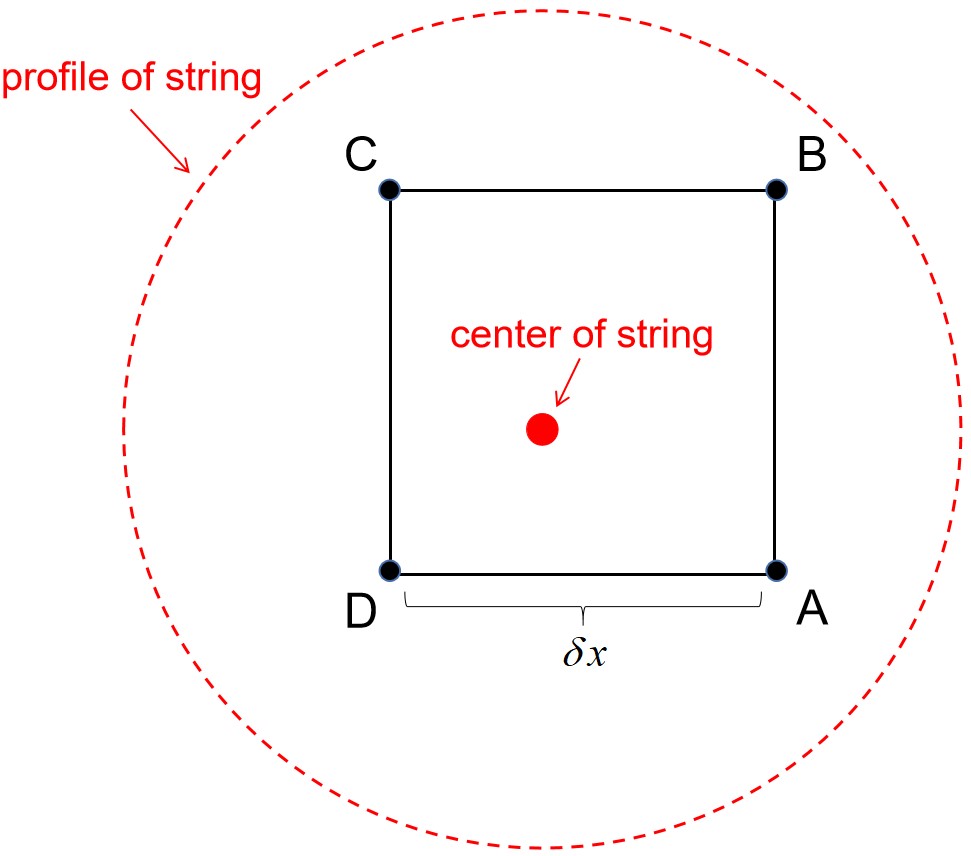
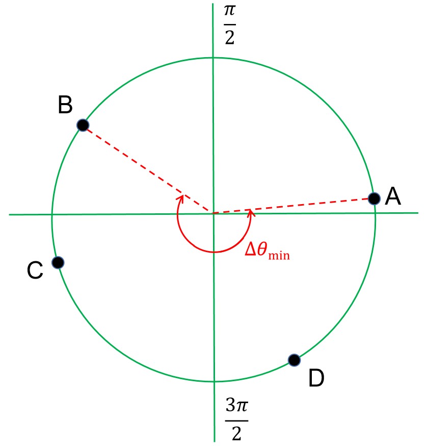
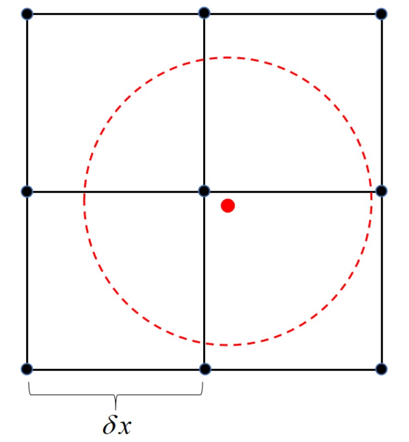
Figure S1: Illustration of the scheme for identifying global string. The left panel shows that a string penetrates a square loop on the lattice. If the center of the string is inside the plaquette and the four points on the plaquette are within the width of the string core, the phase change of the loop around the plaquette should be $2\pi$ due to the property of vortex-like defects. The middle panel shows the phase distribution of the complex scalar field at four points when the string penetrates the square loop, where there is a direction that allows the phase to change continuously and the minimum phase range containing four points is greater than $\pi\ (\Delta\theta_{\rm min}>\pi)$. The right panel illustrates that when the shrinking comoving width of the string is smaller than twice the comoving lattice spacing, it is not reliable to identify the string only by phase.

We can also identify where the domain wall exists according to the phase of the complex scalar field. When considering the non-zero axion mass and $N_{\rm DW}>1$, there will be $N_{\rm DW}$ minima of potential energy located at where $\theta/(2\pi/N_{\rm DW})$ is an integer, with $\theta\in(0,2\pi]$ the phase of $\varphi$ Hiramatsu et al. (2013). The domain wall is located at the boundary with higher potential energy between two minima. Firstly, we assign an integer vacuum number $n_{\rm v}$ to each lattice point to indicate which phase region they belong to. The vacuum number depends on which of the $N_{\rm DW}$ phases that minimize the potential energy is closest to the phase on the lattice point. For example, in the case of $N_{\rm DW}=3$, the three phases that minimize the potential energy are $2\pi/3$, $4\pi/3$, and $2\pi$ in ascending order (see Fig. S2). If the phase of $\varphi$ on a lattice point is $5\pi/6$, it is closest to the first phase which minimizes the potential energy, so the vacuum number is 1. After all the lattice points have been assigned the vacuum number, the domain wall intersects the link between the two adjacent lattice points when the vacuum number of the two lattice points is different.

In the case of $N_{\rm DW}=1$, the identification of domain wall is relatively simple, domain wall intersects the link if $\phi_{1}<0$ and $\phi_{2}$ have different signs at the two ends of the link Hiramatsu et al. (2011b).

To calculate the comoving area density of the domain wall, we first define the quantity $\delta$ that takes the value 1 at both ends of the link intersecting with the domain wall and equals 0 elsewhere. Then, the comoving area density can be expressed as Hiramatsu et al. (2010)

$$A/V=C\sum\limits_{\rm links}\delta\frac{|\nabla\theta|}{|\theta_{,x}|+|\theta_{,y}|+|\theta_{,z}|},$$ (S20)

where $\theta_{,i}\ (i=x,y,z)$ denote the spatial derivatives of the axion field $\theta(\boldsymbol{{\rm x}})$, and $C$ is a parameter chosen to satisfy $A/V=1$ when all the links have the value $\delta=1$.

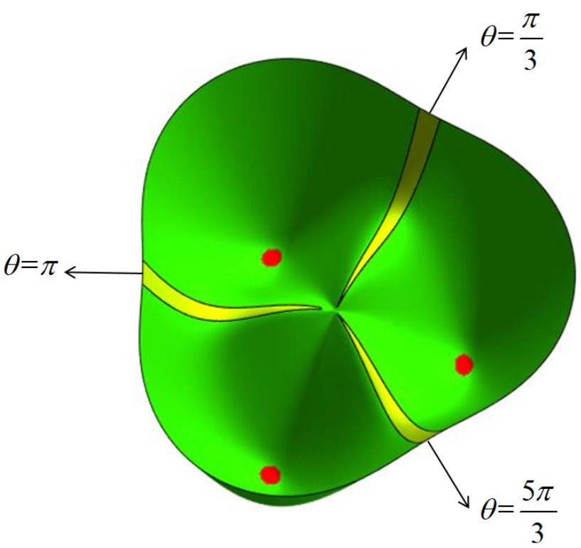
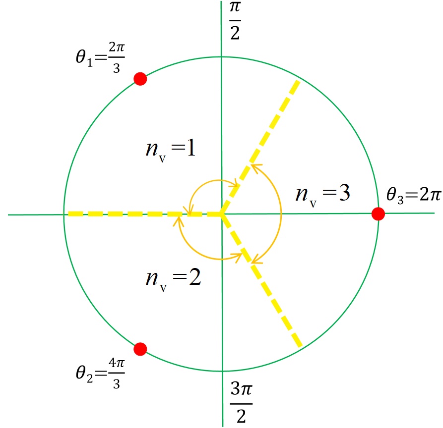
Figure S2: Illustration of the identification of domain walls in the case of $N_{\rm DW}=3$. The left panel shows a top view near the origin of potential, with the red dot indicating the position of potential minimums, and the yellow region representing the location of the domain wall, which is the boundary between the two potential minimums. The right panel interprets how to assign vacuum numbers according to the phase. The potential minimums are located at $\theta_{1}$, $\theta_{2}$ and $\theta_{3}$. Then, divide the entire phase region equally around each minimum, and assign different vacuum numbers to each divided region.

IV Calculation of GW energy density power spectrum

Topological defects with high energy density and non-zero quadrupole moment will cause anisotropic perturbations to the space-time background, while gravitational waves are described by spatial metric perturbations $h_{ij}$ around FLRW background

$${\rm d}s^{2}=-{\rm d}t^{2}+a^{2}(t)(\delta_{ij}+h_{ij}){\rm d}x^{i}{\rm d}x^{j},$$ (S21)

where $t$ denote the cosmic time, $h_{ij}$ are transverse and traceless which satisfying $\partial_{i}h_{ij}=0$ and $h_{ii}=0$.

The energy density of the stochastic GW background radiated by stochastic sources is usually defined as the 00 component of the stress-energy tensor $t_{\mu\nu}$:

$$\rho_{\rm GW}(t)=t_{00}=\frac{1}{32\pi G}\langle\partial_{\mu}{h}_{ij}^{\rm TT}(\boldsymbol{{\rm x}},t)\partial_{\nu}{h}^{{\rm TT},ij}(\boldsymbol{{\rm x}},t)\rangle|_{\mu=\nu=0}=\frac{1}{32\pi G}\langle\dot{h}_{ij}(\boldsymbol{{\rm x}},t)\dot{h}_{ij}(\boldsymbol{{\rm x}},t)\rangle,$$ (S22)

where $G$ is the Newton’s constant, the bracket $\langle...\rangle$ denotes spatial average. In momentum space, when $kV^{\frac{1}{3}}\gg 1$ is satisfied, the GW energy density can be expressed as

$$\rho_{\rm GW}(t) =\frac{1}{32\pi GV}\int_{V}{\frac{d^{3}\boldsymbol{{\rm k}}}{(2\pi)^{3}}\dot{h}_{ij}(\boldsymbol{{\rm k}},t)\dot{h}_{ij}^{*}(\boldsymbol{{\rm k}},t)}$$ (S23)

$$=\frac{1}{32\pi G}\frac{1}{(2\pi)^{3}V}\int{|\boldsymbol{{\rm k}}|^{3}{\rm d(ln}k)}\int{{\rm d}\Omega|\dot{h}_{ij}(\boldsymbol{{\rm k}},t)|^{2}}$$ (S24)

$$\equiv\int{\frac{{\rm d}\rho_{\rm GW}}{{\rm d}{\rm ln}k}{\rm d}{\rm ln}k},$$ (S25)

where ${\rm d}\Omega$ represents a solid angle measure in momentum space. The GW energy density power spectrum is defined as energy density per logarithmic interval and is typically normalized by the critical energy density, $\rho_{c}\equiv 3H^{2}/8\pi G$. The dimensionless GW power spectrum is finally expressed as

$$\Omega_{\rm GW} \equiv\frac{1}{\rho_{c}}\frac{{\rm d}\rho_{\rm GW}}{{\rm dln}k}$$ (S26)

$$=\frac{1}{32\pi G}\frac{1}{(2\pi)^{3}V}\int{{\rm d}\Omega|\boldsymbol{{\rm k}}|^{3}|\dot{h}_{ij}(\boldsymbol{{\rm k}},t)|^{2}}.$$ (S27)

where ${\rm d}\Omega$ represents a solid angle measure in momentum space.

After getting the GW power spectrum at the end time of our simulation, we need to convert it into today’s spectrum. We follow the scheme described in Price and Siemens (2008); Dufaux et al. (2007); Easther et al. (2008). Firstly, due to the increase in spatial volume and the decrease in GW frequency, the GW energy density scales as

$$\frac{\rho_{\rm GW,0}}{\rho_{\rm GW,e}}=\frac{a_{\rm e}^{4}}{a_{0}^{4}}.$$ (S28)

The subscripts ”0” and ”e” denote the quantities today and at the end of our simulation respectively, and the same is true for the following parts. We assume that entropy is always conserved, so the radiation energy density satisfies

$$\frac{\rho_{\rm rad,0}}{\rho_{\rm rad,e}}=\frac{a_{\rm e}^{4}}{a_{0}^{4}}\frac{g_{\rm e}^{1/3}}{g_{0}^{1/3}},$$ (S29)

with $g_{\rm e}(g_{0})$ the number of relativistic degrees of freedom at the end time of simulation (today). For example, we take $g_{\rm e}=81$ at the end of the simulation in the PQ era, while $g_{0}=3.36$. In the radiation-dominated era, the radiation energy density at the end of the simulation is approximately equal to the critical energy density, i.e., $\rho_{\rm rad,e}\approx\rho_{c,\rm e}=3H_{\rm e}^{2}/8\pi G$. Next, we also need to know the frequency of gravitational waves today, which is

$$f_{0} =\frac{k_{\rm p,0}}{2\pi}=\frac{k_{\rm co,e}}{2\pi a_{\rm e}}\frac{a_{\rm e}}{a_{0}}=\frac{k_{\rm co,e}}{2\pi a_{\rm e}}\left(\frac{\rho_{\rm rad,0}}{\rho_{\rm rad,e}}\right)^{1/4}\left(\frac{g_{0}}{g_{\rm e}}\right)^{1/12}$$

$$\approx\frac{k_{\rm co,e}}{a_{\rm e}\rho_{c,\rm e}^{1/4}}\left(\frac{g_{\rm 0}}{g_{\rm e}}\right)^{1/12}\times(5.87\times 10^{10}{\rm Hz})$$ (S30)

where $k_{\rm p,0}$ denote physical momentum today and $k_{\rm co,e}$ denote comoving momentum at the end of our simulation.

The GW power spectrum today can be expressed as

$$\Omega_{\rm GW,0}h^{2} =\frac{h^{2}}{\rho_{c,\rm 0}}\frac{{\rm d}\rho_{\rm GW,0}}{{\rm dln}k_{\rm p,0}}$$

$$=\Omega_{\rm rad,0}h^{2}\left(\frac{g_{\rm 0}}{g_{\rm e}}\right)^{1/3}\left\{\frac{1}{\rho_{c,\rm e}}\frac{{\rm d}\rho_{\rm GW,e}}{{\rm dln}k_{\rm co,e}}\right\},$$ (S31)

where $\Omega_{\rm rad,0}h^{2}=h^{2}\rho_{\rm rad,0}/\rho_{c,\rm 0}\approx 4.3\times 10^{-5}$ is the abundance of radiation today. Note that we multiplied by an additional factor $h^{2}$, to take into account the uncertainty of Hubble expansion rate today.

V Gravitational Waves in the case of $N_{\rm DW}=1$

In the $N_{\rm DW}=1$ case, the gravitational waves are generally expected to be dominated by strings. For the sake of rigor, we investigated the gravitational waves radiated by both pure string networks and string-wall hybrid networks.

To study the gravitational waves radiated by pure strings, we specifically prepared an additional PQ era. For this additional PQ era, we set the PQ vacuum $v_{\rm add}=6\times 10^{16}$ ${\rm GeV}$ to ensure the simulation box can capture large enough Hubble volumes. and our simulation begins at a initial temperature $T_{i}=18T_{\rm c}$. The scalar fields are rescaled with the PQ vacuum $v_{\rm add}$, and the comoving lattice spacing $\delta x$ (and time-step) are rescaled by $w_{*}=a_{i}H_{i}$ with the $a_{i}$ and $H_{i}$ being initial scale factor and Hubble parameter. It is convenient to use the rescaled conformal time $\tilde{\eta}$ $(=\eta/\eta_{i})$ with the initial conformal time being $\eta_{i}=1/w_{*}$ in our simulations. We fix $\tilde{\eta}=1$ to be the initial time at which $T=T_{i}$, so the PQ phase transition happens at $\tilde{\eta}=18$. We evolve the equations of motion in a simulation box of comoving side-length $L_{\rm PQ}=440/(a_{i}H_{i})$ and 1600 points per side. So, the dimensionless comoving lattice spacing is $\delta\tilde{x}=0.275$, and the time-step is chosen as $\delta\tilde{\eta}=0.008$. We continued to evolve the string network until the final moment $\tilde{\eta}_{f}=270$. At the end time, the simulation box contains 4 Hubble volumes to reduce the finite volume effects, and the physical string width $\delta_{\rm st}\sim 1/(\sqrt{\lambda}v_{\rm add})$ is about twice as large as the physical lattice spacing to obtain sufficient resolution (with $\lambda=0.2$).

We use both the definition in Eq. (S17) as well as the standard scaling model Eq. (S19) based on mean string separation to calculate the scaling parameter and achieve consistent results. We first measured the time evolution of mean string separation during the additional PQ era, see left panel of Fig. S3. After a certain period of evolution, the mean string separation increases linearly with cosmic time, indicating that the string networks have entered the scaling regime. By linear fitting, the slope is $\kappa=1.007$. So the scaling parameter is $\xi_{\rm s}=1/\kappa^{2}=0.99$, coherent with the value of scaling parameters calculated by Eq. (S17), see right panel of Fig. S3. The scaling parameters measured under two measurement methods do not exhibit logarithmic increase, consistent with previous studies Yamaguchi et al. (1999); Yamaguchi and Yokoyama (2003); Hiramatsu et al. (2011a); Hiramatsu et al. (2012); Kawasaki et al. (2015); Lopez-Eiguren et al. (2017).

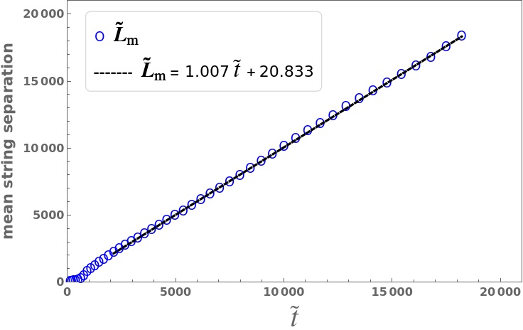
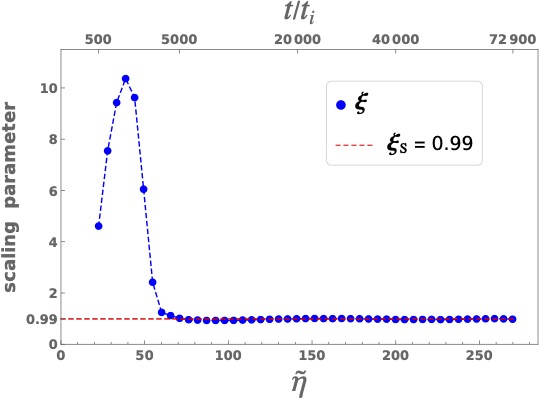
Figure S3: Left panel: Evolution of dimensionless mean string separation ${\tilde{L}_{\rm m}}$ with dimensionless cosmic time $\tilde{t}$ in the additional PQ era. The blue hollow points denote the dimensionless mean string separation calculated according to Eq. (S19). The black dashed line is a linear fit of the mean string separation and time after the string networks have entered the scaling regime. Right panel: Evolution of scaling parameters in rescaled conformal time $\tilde{\eta}$ and rescaled cosmic time $\tilde{t}=t/t_{i}$, with $t_{i}=1/(2H_{i})$ the initial cosmic time. The blue solid points denote the scaling parameter calculated according to Eq. (S17), and the red dashed line is the scaling parameter obtained by global fitting the mean string separation with cosmic time after $\tilde{\eta}=90$ according to the standard scaling model.

We then measured the GW spectrum in the additional PQ era, see FIG. S4. The GW spectrum changes its slope at two characteristic scales, the Hubble length and the string width at the final time, $k_{\rm H}=2\pi H({\tilde{\eta}_{f}})\times a({\tilde{\eta}_{f}})/(a_{i}H_{i})$ and $k_{\rm st}=2\pi/\delta_{\rm st}(\tilde{\eta}_{f})\times a({\tilde{\eta}_{f}})/(a_{i}H_{i})$, with $\delta_{\rm st}(\tilde{\eta}_{f})$ the physical string width. After redshift, the peak amplitude of GW spectrum today is $(\Omega_{\rm GW}h^{2})_{\rm add}=3.81\times 10^{-10}$. For the global (axion) string, the GW spectrum today will follow $\Omega_{\rm GW}h^{2}\propto(v/M_{\rm pl})^{4}$ according to analytic calculations  Fenu et al. (2009), with $M_{\rm pl}$ the full Planck mass. We will then compare this peak amplitude with the peak amplitude of gravitational waves radiated by string-wall hybrid networks with $N_{\rm DW}=1$ in the QCD era, thus verifying whether gravitational waves are dominated by strings.

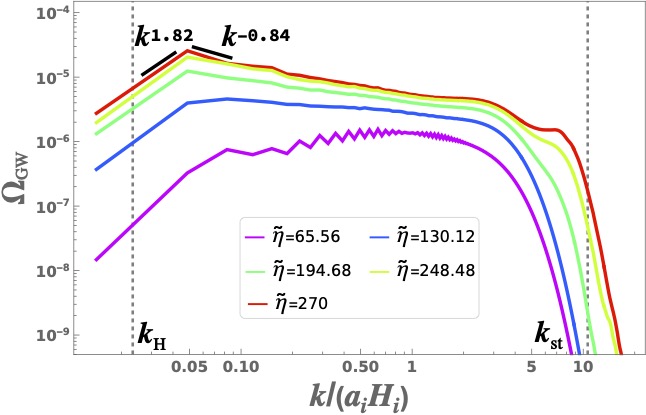
Figure S4: The GW spectrum measured at five different times in the additional PQ era.

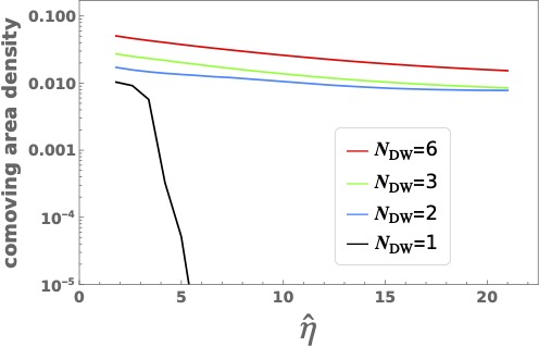
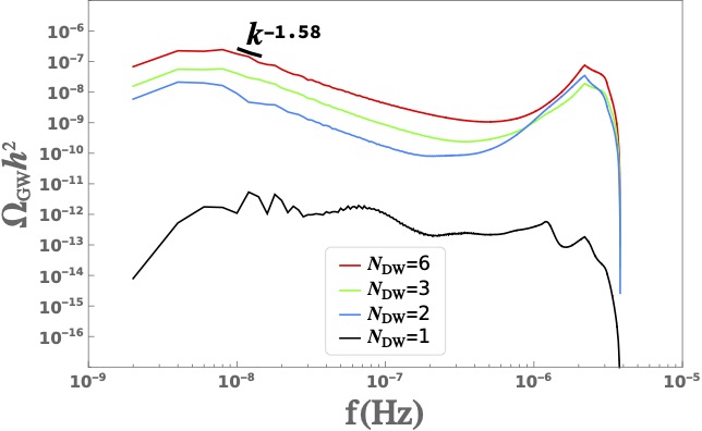
Figure S5: The left panel shows the time evolution of the comoving area density for domain walls at different values of $N_{\rm DW}$ with $\Xi$=0. The right panel shows the GW power spectrum today for different values of $N_{\rm DW}$.

In the QCD era with $N_{\rm DW}=1$, the string-wall network quickly collapses when $H=m$ is satisfied due to the tension of domain walls. The PQ vacuum is reinterpreted as $v_{\rm re}=1.8\times 10^{16}$ GeV. We first measured the comoving area density of the domain wall, see left panel of FIG. S5. Then, from the right panel, the peak amplitude of GW spectrum today in the $N_{\rm DW}=1$ case is $(\Omega_{\rm GW}h^{2})_{\rm QCD}=5.36\times 10^{-12}$. We numerically checked that $(\Omega_{\rm GW}h^{2})_{\rm add}/(\Omega_{\rm GW}h^{2})_{\rm QCD}\approx(v_{\rm add}/v_{\rm re})^{4}$, so $\Omega_{\rm GW}h^{2}\propto(v/M_{\rm pl})^{4}$ is satisfied, indicating GWs are dominated by strings as generally expected. For global string, the GW spectrum today follows $\Omega_{\rm GW}h^{2}\propto(v/M_{\rm pl})^{4}$ according to analytical calculations Fenu et al. (2009), with $M_{\rm pl}$ the full Planck mass. The string(-wall) network quickly collapses due to DW tension when $H(T_{\rm dec})=m$ is satisfied, thus the GW spectrum features the peak frequency $2\pi H(T_{\rm dec})/\rho_{c}^{1/4}(T_{\rm dec})\times(4.54\times 10^{10}){\rm Hz}$, with $\rho_{c}(T_{\rm dec})$ the critical energy density.

We also studied the influence of the domain wall number $N_{\rm DW}$ on the gravitational waves ($N_{\rm DW}=2,3,6$), and found that both the comoving area density and the energy density of gravitational waves are proportional to the domain wall number (see FIG. S5).

References

- Peccei and Quinn (1977a) R. D. Peccei and H. R. Quinn, Phys. Rev. Lett. 38, 1440 (1977a).
- Peccei and Quinn (1977b) R. D. Peccei and H. R. Quinn, Phys. Rev. D 16, 1791 (1977b).
- Wilczek (1978) F. Wilczek, Phys. Rev. Lett. 40, 279 (1978).
- Weinberg (1978) S. Weinberg, Phys. Rev. Lett. 40, 223 (1978).
- Abbott and Sikivie (1983) L. F. Abbott and P. Sikivie, Phys. Lett. B 120, 133 (1983).
- Dine and Fischler (1983) M. Dine and W. Fischler, Phys. Lett. B 120, 137 (1983).
- Preskill et al. (1983) J. Preskill, M. B. Wise, and F. Wilczek, Phys. Lett. B 120, 127 (1983).
- Kawasaki et al. (2015) M. Kawasaki, K. Saikawa, and T. Sekiguchi, Phys. Rev. D 91, 065014 (2015), eprint 1412.0789.
- Hogan and Rees (1988) C. J. Hogan and M. J. Rees, Phys. Lett. B 205, 228 (1988).
- Kolb and Tkachev (1993) E. W. Kolb and I. I. Tkachev, Phys. Rev. Lett. 71, 3051 (1993), eprint hep-ph/9303313.
- Kolb and Tkachev (1994a) E. W. Kolb and I. I. Tkachev, Phys. Rev. D 49, 5040 (1994a), eprint astro-ph/9311037.
- Kolb and Tkachev (1994b) E. W. Kolb and I. I. Tkachev, Phys. Rev. D 50, 769 (1994b), eprint astro-ph/9403011.
- Zurek et al. (2007) K. M. Zurek, C. J. Hogan, and T. R. Quinn, Phys. Rev. D 75, 043511 (2007), eprint astro-ph/0607341.
- Enander et al. (2017) J. Enander, A. Pargner, and T. Schwetz, JCAP 12, 038 (2017), eprint 1708.04466.
- Vaquero et al. (2019) A. Vaquero, J. Redondo, and J. Stadler, JCAP 04, 012 (2019), eprint 1809.09241.
- Buschmann et al. (2020) M. Buschmann, J. W. Foster, and B. R. Safdi, Phys. Rev. Lett. 124, 161103 (2020), eprint 1906.00967.
- Chang and Cui (2023) C.-F. Chang and Y. Cui (2023), eprint 2309.15920.
- Marsh (2016) D. J. E. Marsh, Phys. Rept. 643, 1 (2016), eprint 1510.07633.
- Borsanyi et al. (2016) S. Borsanyi, M. Dierigl, Z. Fodor, S. D. Katz, S. W. Mages, D. Nogradi, J. Redondo, A. Ringwald, and K. K. Szabo, Phys. Lett. B 752, 175 (2016), eprint 1508.06917.
- Hlozek et al. (2015) R. Hlozek, D. Grin, D. J. E. Marsh, and P. G. Ferreira, Phys. Rev. D 91, 103512 (2015), eprint 1410.2896.
- Kawasaki and Nakayama (2013) M. Kawasaki and K. Nakayama, Ann. Rev. Nucl. Part. Sci. 63, 69 (2013), eprint 1301.1123.
- Chang and Cui (2020) C.-F. Chang and Y. Cui, Phys. Dark Univ. 29, 100604 (2020), eprint 1910.04781.
- Chang and Cui (2022) C.-F. Chang and Y. Cui, JHEP 03, 114 (2022), eprint 2106.09746.
- Auclair et al. (2023a) P. Auclair et al. (LISA Cosmology Working Group), Living Rev. Rel. 26, 5 (2023a), eprint 2204.05434.
- Brzeminski et al. (2022) D. Brzeminski, A. Hook, and G. Marques-Tavares, JHEP 11, 061 (2022), eprint 2203.13842.
- Agrawal et al. (2022) P. Agrawal, A. Hook, J. Huang, and G. Marques-Tavares, JHEP 01, 103 (2022), eprint 2010.15848.
- Jain et al. (2021) M. Jain, A. J. Long, and M. A. Amin, JCAP 05, 055 (2021), eprint 2103.10962.
- Jain et al. (2022) M. Jain, R. Hagimoto, A. J. Long, and M. A. Amin, JCAP 10, 090 (2022), eprint 2208.08391.
- Agrawal et al. (2020) P. Agrawal, A. Hook, and J. Huang, JHEP 07, 138 (2020), eprint 1912.02823.
- Dessert et al. (2022) C. Dessert, A. J. Long, and B. R. Safdi, Phys. Rev. Lett. 128, 071102 (2022), eprint 2104.12772.
- Shokair et al. (2014) T. M. Shokair et al., Int. J. Mod. Phys. A 29, 1443004 (2014), eprint 1405.3685.
- Du et al. (2018) N. Du et al. (ADMX), Phys. Rev. Lett. 120, 151301 (2018), eprint 1804.05750.
- Brubaker et al. (2017a) B. M. Brubaker et al., Phys. Rev. Lett. 118, 061302 (2017a), eprint 1610.02580.
- Al Kenany et al. (2017) S. Al Kenany et al., Nucl. Instrum. Meth. A 854, 11 (2017), eprint 1611.07123.
- Brubaker et al. (2017b) B. M. Brubaker, L. Zhong, S. K. Lamoreaux, K. W. Lehnert, and K. A. van Bibber, Phys. Rev. D 96, 123008 (2017b), eprint 1706.08388.
- Caldwell et al. (2017) A. Caldwell, G. Dvali, B. Majorovits, A. Millar, G. Raffelt, J. Redondo, O. Reimann, F. Simon, and F. Steffen (MADMAX Working Group), Phys. Rev. Lett. 118, 091801 (2017), eprint 1611.05865.
- Kahn et al. (2016) Y. Kahn, B. R. Safdi, and J. Thaler, Phys. Rev. Lett. 117, 141801 (2016), eprint 1602.01086.
- Ouellet et al. (2019a) J. L. Ouellet et al., Phys. Rev. Lett. 122, 121802 (2019a), eprint 1810.12257.
- Ouellet et al. (2019b) J. L. Ouellet et al., Phys. Rev. D 99, 052012 (2019b), eprint 1901.10652.
- Chaudhuri et al. (2015) S. Chaudhuri, P. W. Graham, K. Irwin, J. Mardon, S. Rajendran, and Y. Zhao, Phys. Rev. D 92, 075012 (2015), eprint 1411.7382.
- Silva-Feaver et al. (2017) M. Silva-Feaver et al., IEEE Trans. Appl. Supercond. 27, 1400204 (2017), eprint 1610.09344.
- Blasi et al. (2021) S. Blasi, V. Brdar, and K. Schmitz, Phys. Rev. Lett. 126, 041305 (2021), eprint 2009.06607.
- Samanta and Datta (2021) R. Samanta and S. Datta, JHEP 05, 211 (2021), eprint 2009.13452.
- Ellis and Lewicki (2021) J. Ellis and M. Lewicki, Phys. Rev. Lett. 126, 041304 (2021), eprint 2009.06555.
- Bian et al. (2022a) L. Bian, J. Shu, B. Wang, Q. Yuan, and J. Zong, Phys. Rev. D 106, L101301 (2022a), eprint 2205.07293.
- Afzal et al. (2023) A. Afzal et al. (NANOGrav), Astrophys. J. Lett. 951 (2023), eprint 2306.16219.
- Bian et al. (2021) L. Bian, R.-G. Cai, J. Liu, X.-Y. Yang, and R. Zhou, Phys. Rev. D 103, L081301 (2021), eprint 2009.13893.
- Bian et al. (2023) L. Bian, S. Ge, J. Shu, B. Wang, X.-Y. Yang, and J. Zong (2023), eprint 2307.02376.
- Bian et al. (2022b) L. Bian, S. Ge, C. Li, J. Shu, and J. Zong (2022b), eprint 2212.07871.
- Ferreira et al. (2023) R. Z. Ferreira, A. Notari, O. Pujolas, and F. Rompineve, JCAP 02, 001 (2023), eprint 2204.04228.
- Auclair et al. (2023b) P. Auclair, S. Babak, H. Quelquejay Leclere, and D. A. Steer, Phys. Rev. D 108, 043519 (2023b), eprint 2305.11653.
- Boileau et al. (2022) G. Boileau, A. C. Jenkins, M. Sakellariadou, R. Meyer, and N. Christensen, Phys. Rev. D 105, 023510 (2022), eprint 2109.06552.
- Abbott et al. (2021) R. Abbott et al. (LIGO Scientific, Virgo, KAGRA), Phys. Rev. Lett. 126, 241102 (2021), eprint 2101.12248.
- Kibble (1976) T. W. B. Kibble, J. Phys. A 9, 1387 (1976).
- Shellard and Battye (1998) E. P. S. Shellard and R. A. Battye, Phys. Rept. 307, 227 (1998), eprint astro-ph/9808220.
- Sikivie (2008) P. Sikivie, Lect. Notes Phys. 741, 19 (2008), eprint astro-ph/0610440.
- Kim and Carosi (2010) J. E. Kim and G. Carosi, Rev. Mod. Phys. 82, 557 (2010), [Erratum: Rev.Mod.Phys. 91, 049902 (2019)], eprint 0807.3125.
- Yamaguchi et al. (1999) M. Yamaguchi, M. Kawasaki, and J. Yokoyama, Phys. Rev. Lett. 82, 4578 (1999), eprint hep-ph/9811311.
- Yamaguchi and Yokoyama (2003) M. Yamaguchi and J. Yokoyama, Phys. Rev. D 67, 103514 (2003), eprint hep-ph/0210343.
- Hiramatsu et al. (2011a) T. Hiramatsu, M. Kawasaki, T. Sekiguchi, M. Yamaguchi, and J. Yokoyama, Phys. Rev. D 83, 123531 (2011a), eprint 1012.5502.
- Gouttenoire et al. (2020) Y. Gouttenoire, G. Servant, and P. Simakachorn, JCAP 07, 032 (2020), eprint 1912.02569.
- Auclair et al. (2020) P. Auclair et al., JCAP 04, 034 (2020), eprint 1909.00819.
- Dine et al. (1981) M. Dine, W. Fischler, and M. Srednicki, Phys. Lett. B 104, 199 (1981).
- Zhitnitsky (1980) A. R. Zhitnitsky, Sov. J. Nucl. Phys. 31, 260 (1980).
- Kim (1987) J. E. Kim, Phys. Rept. 150, 1 (1987).
- Kim (1979) J. E. Kim, Phys. Rev. Lett. 43, 103 (1979).
- Shifman et al. (1980) M. A. Shifman, A. I. Vainshtein, and V. I. Zakharov, Nucl. Phys. B 166, 493 (1980).
- Sikivie (1982) P. Sikivie, Phys. Rev. Lett. 48, 1156 (1982).
- Zeldovich et al. (1974) Y. B. Zeldovich, I. Y. Kobzarev, and L. B. Okun, Zh. Eksp. Teor. Fiz. 67, 3 (1974).
- Gelmini et al. (1989) G. B. Gelmini, M. Gleiser, and E. W. Kolb, Phys. Rev. D 39, 1558 (1989).
- Larsson et al. (1997) S. E. Larsson, S. Sarkar, and P. L. White, Phys. Rev. D 55, 5129 (1997), eprint hep-ph/9608319.
- Kamionkowski and March-Russell (1992) M. Kamionkowski and J. March-Russell, Phys. Lett. B 282, 137 (1992), eprint hep-th/9202003.
- Holman et al. (1992) R. Holman, S. D. H. Hsu, T. W. Kephart, E. W. Kolb, R. Watkins, and L. M. Widrow, Phys. Lett. B 282, 132 (1992), eprint hep-ph/9203206.
- Dobrescu (1997) B. A. Dobrescu, Phys. Rev. D 55, 5826 (1997), eprint hep-ph/9609221.
- Barr and Seckel (1992) S. M. Barr and D. Seckel, Phys. Rev. D 46, 539 (1992).
- Dine (1992) M. Dine, in Conference on Topics in Quantum Gravity (1992), eprint hep-th/9207045.
- Hiramatsu et al. (2011b) T. Hiramatsu, M. Kawasaki, and K. Saikawa, JCAP 08, 030 (2011b), eprint 1012.4558.
- Liu et al. (2021) J. Liu, R.-G. Cai, and Z.-K. Guo, Phys. Rev. Lett. 126, 141303 (2021), eprint 2010.03225.
- Figueroa et al. (2013) D. G. Figueroa, M. Hindmarsh, and J. Urrestilla, Phys. Rev. Lett. 110, 101302 (2013), eprint 1212.5458.
- Baeza-Ballesteros et al. (2023) J. Baeza-Ballesteros, E. J. Copeland, D. G. Figueroa, and J. Lizarraga (2023), eprint 2308.08456.
- Saurabh et al. (2020) A. Saurabh, T. Vachaspati, and L. Pogosian, Phys. Rev. D 101, 083522 (2020), eprint 2001.01030.
- Hiramatsu et al. (2013) T. Hiramatsu, M. Kawasaki, K. Saikawa, and T. Sekiguchi, JCAP 01, 001 (2013), eprint 1207.3166.
- Wantz and Shellard (2010) O. Wantz and E. P. S. Shellard, Phys. Rev. D 82, 123508 (2010), eprint 0910.1066.
- Grilli di Cortona et al. (2016) G. Grilli di Cortona, E. Hardy, J. Pardo Vega, and G. Villadoro, JHEP 01, 034 (2016), eprint 1511.02867.
- Srednicki (1985) M. Srednicki, Nucl. Phys. B 260, 689 (1985).
- Figueroa et al. (2023) D. G. Figueroa, A. Florio, F. Torrenti, and W. Valkenburg, Comput. Phys. Commun. 283, 108586 (2023), eprint 2102.01031.
- Figueroa et al. (2021) D. G. Figueroa, A. Florio, F. Torrenti, and W. Valkenburg, JCAP 04, 035 (2021), eprint 2006.15122.
- Moore et al. (2002) J. N. Moore, E. P. S. Shellard, and C. J. A. P. Martins, Phys. Rev. D 65, 023503 (2002), eprint hep-ph/0107171.
- Hindmarsh et al. (2020) M. Hindmarsh, J. Lizarraga, A. Lopez-Eiguren, and J. Urrestilla, Phys. Rev. Lett. 124, 021301 (2020), eprint 1908.03522.
- Raffelt (1990) G. G. Raffelt, Phys. Rept. 198, 1 (1990).
- Raffelt (2008) G. G. Raffelt, Lect. Notes Phys. 741, 51 (2008), eprint hep-ph/0611350.
- Gorghetto et al. (2018) M. Gorghetto, E. Hardy, and G. Villadoro, JHEP 07, 151 (2018), eprint 1806.04677.
- Kawasaki et al. (2018) M. Kawasaki, T. Sekiguchi, M. Yamaguchi, and J. Yokoyama, PTEP 2018, 091E01 (2018), eprint 1806.05566.
- Poisson (2008) E. Poisson, Classical and Quantum Gravity 25, 209002 (2008).
- Saikawa (2017) K. Saikawa, Universe 3, 40 (2017), eprint 1703.02576.
- Li et al. (2023) Y. Li, L. Bian, and Y. Jia (2023), eprint 2304.05220.
- Gorghetto et al. (2021) M. Gorghetto, E. Hardy, and H. Nicolaescu, JCAP 06, 034 (2021), eprint 2101.11007.
- O’Hare (2020) C. O’Hare (2020), URL https://cajohare.github.io/AxionLimits/.
- Hiramatsu et al. (2012) T. Hiramatsu, M. Kawasaki, K. Saikawa, and T. Sekiguchi, Phys. Rev. D 85, 105020 (2012), [Erratum: Phys.Rev.D 86, 089902 (2012)], eprint 1202.5851.
- Kolb and Turner (1990) E. W. Kolb and M. S. Turner, The Early Universe, vol. 69 (1990), ISBN 978-0-201-62674-2.
- Fleury and Moore (2016) L. Fleury and G. D. Moore, JCAP 01, 004 (2016), eprint 1509.00026.
- Hiramatsu et al. (2010) T. Hiramatsu, M. Kawasaki, and K. Saikawa, JCAP 05, 032 (2010), eprint 1002.1555.
- Price and Siemens (2008) L. R. Price and X. Siemens, Phys. Rev. D 78, 063541 (2008), eprint 0805.3570.
- Dufaux et al. (2007) J. F. Dufaux, A. Bergman, G. N. Felder, L. Kofman, and J.-P. Uzan, Phys. Rev. D 76, 123517 (2007), eprint 0707.0875.
- Easther et al. (2008) R. Easther, J. T. Giblin, and E. A. Lim, Phys. Rev. D 77, 103519 (2008), eprint 0712.2991.
- Lopez-Eiguren et al. (2017) A. Lopez-Eiguren, J. Lizarraga, M. Hindmarsh, and J. Urrestilla, JCAP 07, 026 (2017), eprint 1705.04154.
- Fenu et al. (2009) E. Fenu, D. G. Figueroa, R. Durrer, and J. Garcia-Bellido, JCAP 10, 005 (2009), eprint 0908.0425.