Time-dependent coupled cluster with orthogonal adaptive basis functions: General formalism and application to the vibrational problem

Abstract

We derive equations of motion for bivariational wave functions with orthogonal adaptive basis sets and specialize the formalism to the coupled cluster ansatz. The equations are related to the biorthogonal case in a transparent way, and similarities and differences are analyzed. We show that the amplitude equations are identical in the orthogonal and biorthogonal formalisms, while the linear equations that determined the basis set time evolution differ by symmetrization. Applying the orthogonal framework to the nuclear dynamics problem, we introduce and implement the orthogonal time-dependent modal vibrational coupled cluster (oTDMVCC) method and benchmark it against exact reference results for four triatomic molecules as well as a 5D trans-bithiophene model. We confirm numerically that the biorthogonal TDMVCC hierarchy converges to the exact solution, while oTDMVCC does not. The differences between TDMVCC and oTDMVCC are found to be small for three of the five cases, but we also identify one case where the formal deficiency of the oTDMVCC approach results in clear and visible errors relative to the exact result. For the remaining example, oTDMVCC exhibits rather modest but visible errors.

I Introduction

The cc method is a highly useful approach for computing the electronic and vibrational structure of molecules. Its benefits include polynomial-scaling cost, size extensivity and fast convergence of the cc hierarchy, leading in many cases to a favorable balance between cost and accuracy. These advantages ultimately stem from the exponential cc parameterization. However, it is also well known that the cc ansatz only works well when the amplitudes are sufficiently small and the reference describes a large part of the wave function. Conversely, if the overlap between the wave function and the reference decreases, the amplitudes grow and the ansatz tends to break down. This kind of situation is easily encountered in explicitly time-dependent or dynamical settings, where large-amplitude motion such as ionization (in electronic structure) or dissociation (in vibrational structure) is commonplace. It is quite obvious that a static reference is ill-suited for describing such processes. However, much less violent phenomena, e.g. the ivr of water, can also lead to the breakdown of the cc ansatz.Madsen et al. (2020a) This weakness of the cc approach can sometimes be alleviated by choosing a dynamical single-particle basis, which in turn induces a dynamical reference that adapts to the wave function at any given time.

Historically, the idea of optimizing the basis set in a cc computation emerged in ground state theory with the so-called bccChiles and Dykstra (1981); Handy et al. (1989); Raghavachari et al. (1990); Hampel, Peterson, and Werner (1992) method. Here, the basis is optimized such that the singles projections vanish (in other words, the singles vanish identically in the Brueckner basis). The bcc theory attracted considerable attention in the 1990s, in part due to a perceived robustness towards symmetry breaking.Stanton, Gauss, and Bartlett (1992); Barnes and Lindh (1994); Xie et al. (1996) It was later discovered that this robustness is not universalCrawford and Stanton (2000) and that the bcc response function contains spurious second-order polesAiga, Sasagane, and Itoh (1994); Koch, Kobayashi, and Jørgensen (1994). bcc has since fallen somewhat out of fashion.

A related idea is to optimize the basis such that the cc energy is minimized. Purvis and Bartlett (1982); Scuseria and Schaefer (1987); Sherrill et al. (1998); Krylov et al. (1998); Pedersen, Koch, and Hättig (1999) When unitary (orthogonal) basis set transformations are used, we will refer to this method as occ (similar acronyms such as OO-CC are also encountered in the literature). In occ, the single excitations are excluded from the outset (i.e. $T=T_{2}+T_{3}+\cdots$), since $\exp(T_{1})$ is redundant with the basis set rotations. Although bcc and occ are conceptually quite similar, it turns out that the occ hierarchy does not converge to the fci limitKöhn and Olsen (2005), which is obviously a disadvantage. For the examples studied by Köhn and OlsenKöhn and Olsen (2005) (ozone and $\mathrm{CH_{2}}$), this deficiency of occ starts to show at the quadruples (OCCDTQ) or quintuples (OCCDTQ5) level. At the doubles (OCCD) and triples (OCCDT) levels, occ and bcc appear to be comparable in accuracy. Pedersen et al.Pedersen, Fernández, and Koch (2001) later introduced nocc. The purpose of using a non-unitary (non-orthogonal) basis set transformation was to simplify response equations, but it was later shown by MyhreMyhre (2018) that nocc does in fact recover the fci limit.

The concept of using optimized or adaptive basis functions for simulating real-time dynamics has a long history in the nuclear dynamics community, where the mctdhMeyer, Manthe, and Cederbaum (1990); Beck et al. (2000) method has been very successful. mctdh employs a complete expansion inside an adaptive active space and thus yields the exact solution for the given choice of space. The analogous electron dynamics method is denoted mctdhf.Zanghellini et al. (2003); Kato and Kono (2004); Nest, Klamroth, and Saalfrank (2005); Caillat et al. (2005) Both of these methods involve an exponentially scaling computational effort, so it is highly relevant to investigate lower-scaling alternatives, e.g. based on the cc ansatz. Real-time time-dependent cc with static basis functions has been considered in the literature for vibrational,Hansen et al. (2019); Hansen, Madsen, and Christiansen (2020); Madsen et al. (2020b) electron,Schönhammer and Gunnarsson (1978); Huber and Klamroth (2011); Pedersen and Kvaal (2019); Skeidsvoll, Balbi, and Koch (2020) and nucleonHoodbhoy and Negele (1978, 1979); Pigg et al. (2012) dynamics (see also Ref. 36 for a recent review), but we will focus specifically on combining adaptive basis functions with the time-dependent cc ansatz. This idea was first taken up in 2012 by Kvaal, who introduced the oatdccKvaal (2012) method for electron dynamics. oatdcc uses biorthogonal adaptive orbitals and also allows the basis to be split into an active and a secondary part (only the active orbitals are correlated). This yields a highly flexible ansatz that converges to the exact limit, i.e. mctdhf. In 2018, Sato et al. proposed the time-dependent OCC (tdocc)Sato et al. (2018) method, which uses orthogonal orbitals and presumably does not converge to the exact limit. However, TD-OCCDT calculations seem to agree very well with higher-level calculations, Sato et al. (2018); Pathak, Sato, and Ishikawa (2020, 2021) which indicates that the use of an orthogonal basis does not introduce large errors in practice.

In the context of nuclear or vibrational dynamics, our group has introduced the tdmvccMadsen et al. (2020a) method, which uses an adaptive active space inspired by mctdh (formally speaking, tdmvcc can be considered a vibrational analogue of oatdcc). Again, the use of a biorthogonal basis guarantees the convergence to the exact solution, i.e. mctdh.

Splitting a biorthogonal basis into active and secondary parts leads to the peculiar situation that the active ket and bra bases are allowed to span different spaces. Although it is consistent with the formalism, we have found that this feature sometimes leads to numerical instability.Højlund et al. (2022) In Ref. 41 we proposed a scheme that effectively locks the active bra and ket spaces together, while still allowing non-unitary transformations within the active space. Although this scheme was shown to solve the stability problem without sacrificing accuracy, we certainly feel there is more to be learned about time-dependent cc with adaptive basis functions. In this paper we therefore consider the use of orthogonal, adaptive basis functions in vibrational cc. The resulting method (which is analogous to tdocc) is denoted orthogonal tdmvcc, or otdmvcc for short.

Time-dependent cc equations are often derived using Arponen’s tdbvpArponen (1983). The original version of this principle uses a complex-valued action, which must be a holomorphic or complex analytic function of the wave function parameters, as explained by KvaalKvaal (2012). We will see that the use of an orthogonal basis leads to a non-holomorphic action, which has some important mathematical consequences that are best explained using the terminology of complex analysisStein and Shakarchi (2003). For the convenience of the reader and for the clarity of our exposition, we provide a brief overview of some aspects of complex analysis (see Appendix A) that we will use throughout the paper.

The paper is organized as follows: Section II covers the theory, including the tdbvp for holomorphic and non-holomorphic parameterizations and derivations of the eom. This is followed by a brief description of our computer implementation in Sec. III and a few numerical examples in Sec. IV. Section V summarizes our findings and concludes with an outlook on future work.

II Theory

II.1 The time-dependent bivariational principle

In Ref. 41, we considered a complex bivariational Lagrangian,

$$\mathcal{L}=\langle\Psi^{\prime}|(i\partial_{t}-H)|\Psi\rangle=\mathcal{L}(\mathbf{y},\dot{\mathbf{y}},t),$$ (1)

where the bra and ket states are formally independent. We showed the well-known fact that stationary points ($\delta\mathcal{S}=0$) of the action-like functional

$$\mathcal{S}=\int_{t_{0}}^{t_{1}}\mathcal{L}\differential{t}$$ (2)

correspond to the solutions of a set of ele,

$$0=\partialderivative{\mathcal{L}}{y_{i}}-\derivative{t}\partialderivative{\mathcal{L}}{\dot{y}_{i}},$$ (3)

for the wave function parameters $y_{i}$. This formalism requires the Lagrangian to be a complex analytic or holomorphicStein and Shakarchi (2003) function of the complex parameters $y_{i}$, implying that complex conjugation cannot appear in the wave function parameterization.Kvaal (2012) This restriction rules out the use of orthogonal basis sets, since in that case the bra basis functions are simply the complex conjugate of the ket basis functions. Instead, one should a biorthogonal basis.

One might be tempted to ignore these formal considerations and simply write down $\mathcal{L}$ with an orthogonal basis set, which would then make $\mathcal{L}$ a complex-valued, non-holomorphic function. As explained in Appendix A, we can consider such a function $\mathcal{L}$ as depending on $y_{i}$ and $y_{i}^{*}$, which are treated as independent variables. Making the corresponding action-like functional stationary again leads to a set of ele,

$$0 =\partialderivative{\mathcal{L}}{y_{i}}-\derivative{t}\partialderivative{\mathcal{L}}{\dot{y}_{i}},$$ (4a)

$$0 =\partialderivative{\mathcal{L}}{y_{i}^{*}}-\derivative{t}\partialderivative{\mathcal{L}}{\dot{y}_{i}^{*}}.$$ (4b)

The trouble is that these equations are not each other’s complex conjugate since $\mathcal{L}$ is complex. As an example, note that

$$\left(\partialderivative{\mathcal{L}}{y_{i}}\right)^{\!*}=\partialderivative{\mathcal{L}^{*}}{y_{i}^{*}}\neq\partialderivative{\mathcal{L}}{y_{i}^{*}}.$$ (5)

The consequence is that Eqs. (4) do not have a consistent solution (this kind of situation is also explained in Appendix A). We can attempt to solve Eqs. (4) while treating $y_{i}$ and $y_{i}^{*}$ as truly independent, but the solution will not respect the obvious requirement that $(\mathrm{d}y_{i}/\mathrm{d}t)^{*}=(\mathrm{d}y_{i}^{*}/\mathrm{d}t)$, i.e. complex conjugate pairs do not remain each other’s complex conjugate. Such a formalism is thus inconsistent, as also noted by KvaalKvaal (2012).

In this paper we consider instead a manifestly real Lagrangian,

$$\bar{\mathcal{L}}=\tfrac{1}{2}(\mathcal{L}+\mathcal{L}^{*})=\bar{\mathcal{L}}(\mathbf{y},\dot{\mathbf{y}},\mathbf{y}^{*},\dot{\mathbf{y}}^{*},t),$$ (6)

that depends on the wave function parameters, the complex conjugate parameters and the time derivative of both. As usual, we define an action-like functional,

$$\bar{\mathcal{S}}=\int_{t_{0}}^{t_{1}}\bar{\mathcal{L}}\differential{t},$$ (7)

which is made stationary ($\delta\bar{\mathcal{S}}=0$) with respect to variations in the parameters $y_{i}$ and the complex conjugate parameters $y_{i}^{*}$. The resulting ele are:

$$0 =\partialderivative{\bar{\mathcal{L}}}{y_{i}}-\derivative{t}\partialderivative{\bar{\mathcal{L}}}{\dot{y}_{i}},$$ (8a)

$$0 =\partialderivative{\bar{\mathcal{L}}}{y_{i}^{*}}-\derivative{t}\partialderivative{\bar{\mathcal{L}}}{\dot{y}_{i}^{*}}.$$ (8b)

Since $\bar{\mathcal{L}}$ is real, the two sets of ele are exactly each other’s complex conjugate ensuring that the eom for $y_{i}$ and $y_{i}^{*}$ are also each other’s complex conjugate in the sense that $(\mathrm{d}y_{i}/\mathrm{d}t)^{*}=(\mathrm{d}y_{i}^{*}/\mathrm{d}t)$. Having settled this point, we only need to solve either Eq. (8a) or (8b). Real Lagrangians like Eq. (6) have previously been considered in the literature. Pedersen and Koch (1997, 1998); Sato et al. (2018); Kristiansen et al. (2022)

It is quite possible some parameters $\alpha_{i}\in\mathbf{y}$ appear only as $\alpha_{i}$ and never as $\alpha_{i}^{*}$ in the bra and ket states, meaning $\mathcal{L}$ is a holomorphic function of $\alpha_{i}$. In that case the ele of Eq. (8a) simplify in the following way:

$$0 =\partialderivative{\bar{\mathcal{L}}}{\alpha_{i}}-\derivative{t}\partialderivative{\bar{\mathcal{L}}}{\dot{\alpha}_{i}}$$

$$=\frac{1}{2}\left(\partialderivative{\mathcal{L}}{\alpha_{i}}-\derivative{t}\partialderivative{\mathcal{L}}{\dot{\alpha}_{i}}\right)+\frac{1}{2}\left(\partialderivative{\mathcal{L}}{\alpha_{i}^{*}}-\derivative{t}\partialderivative{\mathcal{L}}{\dot{\alpha}_{i}^{*}}\right)^{*}$$

$$=\frac{1}{2}\left(\partialderivative{\mathcal{L}}{\alpha_{i}}-\derivative{t}\partialderivative{\mathcal{L}}{\dot{\alpha}_{i}}\right)$$ (9)

We recover a set of ele based on the complex Lagrangian $\mathcal{L}$, which we will refer to as being complex bivariational. Similarly, we will use the term real bivariational when referring to equations based on the real Lagrangian. Equation (9) then shows that the real and complex bivariational principles are equivalent for the special subset of parameters $\alpha_{i}$. For parameterizations that are holomorphic in all parameters, e.g. time-dependent cc with static basis functions, the two principles yield fully equivalent eom.

II.2 Parameterization

II.2.1 Time-dependent basis sets

The wave function is parameterized using time-dependent orthonormal basis functions (denoted modals or orbitals), that are in turn expanded in a primitive orthonormal basis. Rather than working directly with the concrete basis functions, we employ a sq formalism for vibrational structureChristiansen (2004) based on creation and annihilation operators (not ladder operators) that obey the following commutator relations:

$$[a^{m^{\smash{\prime}}}_{\mspace{-1.0mu}\alpha^{m^{\smash{\prime}}}},a^{m\mspace{-0.5mu}\raisebox{0.90417pt}{$\scriptstyle\dagger$}}_{\mspace{0.0mu}\beta^{m}}] =\delta_{mm^{\prime}}\delta_{\alpha^{m}\beta^{m}}$$ (10a)

$$[a^{m^{\smash{\prime}}}_{\mspace{-1.0mu}\alpha^{m^{\smash{\prime}}}},a^{m}_{\mspace{0.0mu}\beta^{m}}] =0$$ (10b)

$$[a^{m^{\smash{\prime}}\mspace{-0.5mu}\raisebox{1.80835pt}{$\scriptstyle\dagger$}}_{\mspace{0.0mu}\alpha^{m^{\smash{\prime}}}},a^{m\mspace{-0.5mu}\raisebox{0.90417pt}{$\scriptstyle\dagger$}}_{\mspace{0.0mu}\beta^{m}}] =0.$$ (10c)

We use indices $m$ and $m^{\prime}$ to enumerate the vibrational modes (which are distinguishable degrees of freedom), while the indices $\alpha^{m}$ and $\beta^{m}$ indicate the modal basis functions for each individual mode. The well-known electronic structure sq formalismHelgaker, Jørgensen, and Olsen (2000) is defined in terms of anti-commutators rather than commutators, which reflects the very different physical nature of electronic and nuclear motion. However, the one-mode shift operators,

$$E^{m}_{{\alpha}^{m}{\beta}^{m}}=a^{m\mspace{-0.5mu}\raisebox{0.90417pt}{$\scriptstyle\dagger$}}_{\mspace{0.0mu}\alpha^{m}}a^{m}_{\mspace{0.0mu}\beta^{m}},$$ (11)

satisfy essentially the same commutator as their electronic counterparts:

$$[E^{m}_{{\alpha}^{m}{\beta}^{m}},E^{m^{\prime}}_{{\gamma}^{m^{\smash{\prime}}}\!{\delta}^{m^{\smash{\prime}}}}]=\delta_{mm^{\prime}}(\delta_{\beta^{m}\gamma^{m}}E^{m}_{{\alpha}^{m}{\delta}^{m}}-\delta_{\alpha^{m}\delta^{m}}E^{m}_{{\gamma}^{m}{\beta}^{m}}).$$ (12)

This means that our derivations carry over to electronic structure after removing mode indices as appropriate.

$$\tilde{a}^{m\mspace{-0.5mu}\raisebox{0.90417pt}{$\scriptstyle\dagger$}}_{\mspace{0.0mu}p^{m}}=\sum_{\alpha}a^{m\mspace{-0.5mu}\raisebox{0.90417pt}{$\scriptstyle\dagger$}}_{\mspace{0.0mu}\alpha^{m}}V^{m}_{\mspace{-2.0mu}\alpha^{m}p^{m}}.$$ (13)

The tilde on the left-hand side indicates the time-dependence of the creation operator. We use $\alpha^{m}$, $\beta^{m}$ to denote primitive indices, while $p^{m}$, $q^{m}$, $r^{m}$, $s^{m}$ denote generic time-dependent indices. The time-dependent basis is split into an active basis indexed by $t^{m}$, $u^{m}$, $v^{m}$, $w^{m}$ and a secondary basis indexed by $x^{m}$, $y^{m}$. We use the symbols $N$ and $N_{\mspace{-2.0mu}\mathrm{\scriptscriptstyle A}}$ for the total number of basis functions per mode and the number of active basis functions per mode, respectively. Collecting the basis set coefficients in square matrices $\mathbf{V}^{m}$, we obtain the following block structure:

$$\mathbf{V}^{m} =\left[\begin{array}[]{c | c}{\mathbf{V}^{m}_{\!\!\mathrm{\scriptscriptstyle A}}}&\,\mathbf{V}^{m}_{\!\!\mathrm{\scriptscriptstyle S}}\rule[-4.30554pt]{0.0pt}{0.0pt}\end{array}\right].$$ (15)

Using the same matrix notation, we write the orthonormality constraint as

$$\mathbf{V}^{m\dagger}\,\mathbf{V}^{m}=\mathbf{1}^{m}.$$ (16)

We also need to consider the corresponding consistency conditionsDirac (1950); Ohta (2000, 2004), i.e. the time derivative of the constraints:

$$\mathbf{0}=\dot{\mathbf{V}}^{m\dagger}\,\mathbf{V}^{m}+\mathbf{V}^{m\dagger}\,\dot{\mathbf{V}}^{m}.$$ (17)

The consistency conditions are trivially satisfied if

$$\dot{\mathbf{V}}^{m\dagger}\,\mathbf{V}^{m} =+i\mathbf{G}^{m},$$ (18a)

$$\mathbf{V}^{m\dagger}\,\dot{\mathbf{V}}^{m} =-i\mathbf{G}^{m},$$ (18b)

where $\mathbf{G}^{m}$ is a Hermitian but otherwise arbitrary time-dependent matrix, which is typically denoted the constraint matrix. The corresponding constraint operator is defined as

$$g=\sum_{m}g^{m}=\sum_{m}\sum_{p^{m}q^{m}}g^{m}_{{p}^{m}{q}^{m}}\tilde{E}^{m}_{{p}^{m}{q}^{m}}.$$ (19)

Using Eq. (18b) and the unitarity of $\mathbf{V}^{m}$ now yields the eom for the basis set coefficients,

$$i\dot{\mathbf{V}}^{m}=\mathbf{V}^{m}\mathbf{G}^{m}.$$ (20)

This shows that the time evolution of the basis set is generated by the constraint matrices, which must be determined from the basis set ele.

II.2.2 Wave function expansion

We consider wave function expansions of the form

$$\ket{\Psi} =\ket{\Psi(\bm{\alpha},\mathbf{V})},$$ (21a)

$$\bra{\Psi^{\prime}} =\bra{\Psi^{\prime}(\bm{\alpha},\mathbf{V}^{*})}$$ (21b)

where $\bm{\alpha}$ denotes a vector of complex configurational parameters as opposed to the basis set parameters $\mathbf{V}=\{\mathbf{V}^{m}\}$. We make the restriction from the outset that the bra and ket states depend only on $\bm{\alpha}$ and not on $\bm{\alpha}^{*}$. The ket state depends on the basis set coefficients $\mathbf{V}$ themselves, while the bra state depends only on the complex conjugate basis set coefficients, as indicated in Eq. (21b). Finally, the wave function is required to be contained in the active space, i.e. the space spanned by the active basis functions. Although this means that the secondary basis functions are not explicitly present in the wave function, we find it instructive to derive eom for the full matrices $\mathbf{V}^{m}$, including the active and secondary blocks.

II.3 Equations of motion

II.3.1 Configurational parameters

The Lagrangian is (by ansatz) a holomorphic function of the configurational parameters $\alpha_{i}$, so the real bivariational ele (based on $\bar{\mathcal{L}}$) simplify to a set of complex bivariational ele (based on $\mathcal{L}$) as shown in Eq. (9). The complex bivariational case was considered in Ref. 41, so rather than deriving the eom from scratch, we simply cite the result:

$$i\dot{\alpha}_{i} =\sum_{j}(\mathbf{M}^{-1})_{ij}\bigg{(}h_{j}-\sum_{m}\sum_{p^{m}q^{m}}A_{{j}({m}\,{p}^{m}{q}^{m})}g^{m}_{{p}^{m}{q}^{m}}\bigg{)}$$ (22)

Here, we have defined an anti-symmetric matrix $\mathbf{M}$ with elements

$$M_{ij}=\Big{\langle}\partialderivative{\Psi^{\prime}}{\alpha_{i}}\mspace{2.0mu}\Big{|}\mspace{1.5mu}\partialderivative{\Psi}{\alpha_{j}}\Big{\rangle}-\Big{\langle}\partialderivative{\Psi^{\prime}}{\alpha_{j}}\mspace{2.0mu}\Big{|}\mspace{1.5mu}\partialderivative{\Psi}{\alpha_{i}}\Big{\rangle}$$ (23)

and a vector $\mathbf{h}$ that contains energy derivatives:

$$h_{i} =\partialderivative{\mathcal{H}}{\alpha_{i}},\quad\mathcal{H}=\langle\Psi^{\prime}|H|\Psi\rangle.$$ (24)

The matrix $\mathbf{A}$ holds derivatives of the one-mode density matrices,

$$A_{{j}({m}\,{p}^{m}{q}^{m})} =\partialderivative{\rho^{m}_{\mspace{0.0mu}q^{m}p^{m}}}{\alpha_{j}},\quad\rho^{m}_{\mspace{0.0mu}q^{m}p^{m}}=\langle\Psi^{\prime}|\tilde{E}^{m}_{{p}^{m}{q}^{m}}|\Psi\rangle.$$ (25)

The notation $(m\,p^{m}q^{m})$ is understood to denote a single compound index.

II.3.2 Basis set parameters

Before considering the basis set equations derived from the real Lagrangian $\bar{\mathcal{L}}$, we recall the analogous equations from Ref. 41:

$$\mathbf{0}=\mathbf{F}^{m}-\big{(}\bm{\rho}^{m}\mathbf{G}^{m}-\mathbf{G}^{m}\bm{\rho}^{m}\big{)}+i\dot{\bm{\rho}}^{m},$$ (26)

The matrix $\mathbf{F}^{m}$ has elements

$$F^{m}_{{q}^{m}{p}^{m}} =\langle\Psi^{\prime}|[H,\tilde{E}^{m}_{{p}^{m}{q}^{m}}]|\Psi\rangle$$

$$=\langle\Psi^{\prime}|[H,\tilde{a}^{m\mspace{-0.5mu}\raisebox{0.90417pt}{$\scriptstyle\dagger$}}_{\mspace{0.0mu}p^{m}}]\tilde{a}^{m}_{\mspace{0.0mu}q^{m}}|\Psi\rangle-\langle\Psi^{\prime}|\tilde{a}^{m\mspace{-0.5mu}\raisebox{0.90417pt}{$\scriptstyle\dagger$}}_{\mspace{0.0mu}p^{m}}[\tilde{a}^{m}_{\mspace{0.0mu}q^{m}},H]|\Psi\rangle$$ (27)

and is thus the difference between the generalized mean-field or Fock matrices $\tilde{\mathbf{F}}^{\prime m}$ and $\tilde{\mathbf{F}}^{m}$:

$$\tilde{F}^{\prime m}_{{q}^{m}{p}^{m}} =\langle\Psi^{\prime}|[H,\tilde{a}^{m\mspace{-0.5mu}\raisebox{0.90417pt}{$\scriptstyle\dagger$}}_{\mspace{0.0mu}p^{m}}]\tilde{a}^{m}_{\mspace{0.0mu}q^{m}}|\Psi\rangle,$$ (28a)

$$\tilde{F}^{m}_{{q}^{m}{p}^{m}} =\langle\Psi^{\prime}|\tilde{a}^{m\mspace{-0.5mu}\raisebox{0.90417pt}{$\scriptstyle\dagger$}}_{\mspace{0.0mu}p^{m}}[\tilde{a}^{m}_{\mspace{0.0mu}q^{m}},H]|\Psi\rangle.$$ (28b)

We showed in Ref. 41 that the element indexed by $(q^{m}p^{m})$ of the complex bivariational constraint equations, Eq. (26), can be written as

$$\sum_{m^{\prime}}\sum_{r^{m^{\prime}}s^{m^{\prime}}}\bigg{[}C_{({m}\,{p}^{m}{q}^{m})({m^{\prime}}{r}^{m^{\smash{\prime}}}\!{s}^{m^{\smash{\prime}}})}+\sum_{ij}A_{{i}({m}\,{p}^{m}{q}^{m})}(\mathbf{M}^{-1})_{ij}A_{{j}({m^{\prime}}{r}^{m^{\smash{\prime}}}\!{s}^{m^{\smash{\prime}}})}\bigg{]}g^{m^{\prime}}_{{r}^{m^{\smash{\prime}}}\!{s}^{m^{\smash{\prime}}}}\\ =\langle\Psi^{\prime}|[H,\tilde{E}^{m}_{{p}^{m}{q}^{m}}]|\Psi\rangle+\sum_{ij}A_{{i}({m}\,{p}^{m}{q}^{m})}(\mathbf{M}^{-1})_{ij}h_{j}$$ (29)

with the definition

$$C_{({m}\,{p}^{m}{q}^{m})({m^{\prime}}{r}^{m^{\smash{\prime}}}\!{s}^{m^{\smash{\prime}}})} =\langle\Psi^{\prime}|[\tilde{E}^{m^{\prime}}_{{r}^{m^{\smash{\prime}}}\!{s}^{m^{\smash{\prime}}}},\tilde{E}^{m}_{{p}^{m}{q}^{m}}]|\Psi\rangle$$

$$=\delta_{mm^{\prime}}(\delta_{s^{m}p^{m}}\rho^{m}_{\mspace{0.0mu}q^{m}r^{m}}-\delta_{r^{m}q^{m}}\rho^{m}_{\mspace{0.0mu}s^{m}p^{m}}).$$ (30)

In matrix notation, Eq. (29) reads

$$(\mathbf{C}+\mathbf{A}^{\mspace{-3.0mu}\mathsf{T}}\mathbf{M}^{-1}\mathbf{A})\mathbf{g}=\mathbf{f}+\mathbf{A}^{\mspace{-3.0mu}\mathsf{T}}\mathbf{M}^{-1}\mathbf{h}$$ (31)

or, even more compactly,

$$\mathbf{C}^{\prime}\mathbf{g}=\mathbf{f}^{\prime}\mathbf{h}.$$ (32)

The vector $\mathbf{g}$ simply contains all constraint elements for all modes. Equation (32) leads to generic or non-Hermitian (i.e. neither Hermitian nor anti-Hermitian) constraint matrices and biorthonormal basis functions.

The real Lagrangian considered in this paper leads to Hermitian constraint matrices and orthonormal basis functions. The derivation of the constraint equations is not complicated and can be found in Appendix B. The result simply reads

$$\mathbf{0} =\mathbb{A}\Big{[}\mathbf{F}^{m}-\big{(}\bm{\rho}^{m}\mathbf{G}^{m}-\mathbf{G}^{m}\bm{\rho}^{m}\big{)}+i\dot{\bm{\rho}}^{m}\Big{]},$$ (33)

where $\mathbb{A}[\,\cdot\,]$ denotes the anti-Hermitian part of a square matrix (later, we will use $\mathbb{H}[\,\cdot\,]$ for the Hermitian part). It is interesting to note that Eq. (33) (derived from a real Lagrangian) is exactly the anti-Hermitian part of Eq. (26) (derived from a complex Lagrangian). This shows very clearly how the symmetrization of the Lagrangian induces a symmetrization of the constraint equations.

The elementwise representation of Eq. (33) is obtained by taking element $(q^{m}p^{m})$ of Eq. (29), subtracting from it the complex conjugate of element $(p^{m}q^{m})$ and multiplying the result by one half. Using the fact that the constraint matrices are Hermitian, the result reads

$$\sum_{m^{\prime}}\sum_{r^{m^{\prime}}s^{m^{\prime}}}\begin{aligned} t]{2}\frac{1}{2}\bigg{[}\;&C_{({m}\,{p}^{m}{q}^{m})({m^{\prime}}{r}^{m^{\smash{\prime}}}\!{s}^{m^{\smash{\prime}}})}{}+{}&&\sum_{ij}A_{{i}({m}\,{p}^{m}{q}^{m})}(\mathbf{M}^{-1})_{ij}A_{{j}({m^{\prime}}{r}^{m^{\smash{\prime}}}\!{s}^{m^{\smash{\prime}}})}\\ -&C_{({m}\,{q}^{m}{p}^{m})({m^{\prime}}{s}^{m^{\smash{\prime}}}\!{r}^{m^{\smash{\prime}}})}^{*}{}-{}&&\sum_{ij}A_{{i}({m}\,{q}^{m}{p}^{m})}^{*}(\mathbf{M}^{-1})^{*}_{ij}A_{{j}({m^{\prime}}{s}^{m^{\smash{\prime}}}\!{r}^{m^{\smash{\prime}}})}^{*}\bigg{]}g^{m^{\prime}}_{{r}^{m^{\smash{\prime}}}\!{s}^{m^{\smash{\prime}}}}\end{aligned}\\ \begin{aligned} t]{3}=\;\frac{1}{2}\bigg{[}&\langle\Psi^{\prime}|[H,\tilde{E}^{m}_{{p}^{m}{q}^{m}}]|\Psi\rangle{}&&+{}&&\sum_{ij}A_{{i}({m}\,{p}^{m}{q}^{m})}(\mathbf{M}^{-1})_{ij}h_{j}\\ -&\langle\Psi^{\prime}|[H,\tilde{E}^{m}_{{q}^{m}{p}^{m}}]|\Psi\rangle^{*}{}&&-{}&&\sum_{ij}A_{{i}({m}\,{q}^{m}{p}^{m})}^{*}(\mathbf{M}^{-1})_{ij}^{*}h_{j}^{*}\bigg{]}.\end{aligned}$$ (34)

Note how the modal indices are exchanged in the complex conjugate terms:

$$(p^{m}q^{m}) \rightarrow(q^{m}p^{m}),$$

$$(r^{m^{\prime}}s^{m^{\prime}}) \rightarrow(s^{m^{\prime}}r^{m^{\prime}}).$$ (35)

This exchange of indices can be performed by a block diagonal permutation matrix $\mathbf{S}$ with elements

$$S_{({m}\,{p}^{m}{q}^{m})({m^{\prime}}{r}^{m^{\smash{\prime}}}\!{s}^{m^{\smash{\prime}}})} =\delta_{mm^{\prime}}S^{m}_{(p^{m}q^{m})(r^{m}s^{m})},$$ (36a)

$$S^{m}_{(p^{m}q^{m})(r^{m}s^{m})} =\delta_{p^{m}s^{m}}\delta_{q^{m}r^{m}}.$$ (36b)

This allows us to write Eq. (34) as

$$\tfrac{1}{2}(\mathbf{C}^{\prime}-\mathbf{S}\mathbf{C}^{\prime*}\mathbf{S})\mathbf{g}=\tfrac{1}{2}(\mathbf{f}^{\prime}-\mathbf{S}\mathbf{f}^{\prime*})$$ (37)

or, with obvious definitions,

$$\bar{\mathbf{C}}^{\prime}\mathbf{g}=\bar{\mathbf{f}}^{\prime}.$$ (38)

It is easy to verify that $\mathbf{S}=\mathbf{S}^{-1}=\mathbf{S}^{\mspace{-3.0mu}\mathsf{T}}$, which enables a concise statement of the symmetries of Eq. (38):

$$\mathbf{S}\bar{\mathbf{C}}^{\prime}\mathbf{S} =-\mathbf{C}^{\prime*},$$ (39a)

$$\mathbf{S}\bar{\mathbf{f}}^{\prime} =-\mathbf{f}^{\prime*}.$$ (39b)

These symmetries embody the Hermiticity of the constraint matrices. Table 1 provides an overview of the effect of symmetrizing the Lagrangian.

Table 1: Effect of symmetrizing the Lagrangian. See text for definitions.

	Complex Lagrangian	Real Lagrangian
Lagrangian	$\mathcal{L}$	$\tfrac{1}{2}(\mathcal{L}+\mathcal{L}^{*})$
Basis set	Biorthogonal	Orthogonal
Constraint matrix	Generic	Hermitian
Ket basis evolution	$\dot{\mathbf{U}}^{m}=-i\mathbf{U}^{m}\mathbf{G}^{m}$	$\dot{\mathbf{V}}^{m}=-i\mathbf{V}^{m}\mathbf{G}^{m}$
Bra basis evolution	$\dot{\mathbf{W}}^{m}=+i\mathbf{G}^{m}\mathbf{U}^{m}$	$\dot{\mathbf{V}}^{m\dagger}=+i\mathbf{G}^{m}\mathbf{V}^{m\dagger}$
Constraint eqs. (a)	$\mathbf{0}=\mathbf{F}^{m}-\big{(}\bm{\rho}^{m}\mathbf{G}^{m}-\mathbf{G}^{m}\bm{\rho}^{m}\big{)}+i\dot{\bm{\rho}}^{m}$	$\mathbf{0}=\mathbb{A}\big{[}\mathbf{F}^{m}-\big{(}\bm{\rho}^{m}\mathbf{G}^{m}-\mathbf{G}^{m}\bm{\rho}^{m}\big{)}+i\dot{\bm{\rho}}^{m}\big{]}$
Constraint eqs. (b)	$\mathbf{C}^{\prime}\mathbf{g}=\mathbf{f}^{\prime}\mathbf{h}$	$(\mathbf{C}^{\prime}-\mathbf{S}\mathbf{C}^{\prime*}\mathbf{S})\mathbf{g}=\mathbf{f}^{\prime}-\mathbf{S}\mathbf{f}^{\prime*}$

II.3.3 Analysis of the basis set equations

Before performing the analysis, it is convenient to introduce some notation to denote various kinds of indices and pairs of indices; see Figs. 1 and 2. The vibrational case differs from the electronic case by having a separate basis set for each mode (and thus a separate set of indices) and by having only one reference (or occupied) index per mode. These differences have some consequences in terms of the concrete appearance of the final working equations. The general analysis, however, remains valid in both cases.

Figure 1: Summary of index conventions used throughout the text.

Figure 2: Summary of index pair conventions used throughout the text.

With the notation in place, we need to consider the different blocks of Eq. (34). The first important point is that

$$A_{{i}({m}\,{p}^{m}{q}^{m})}=\partialderivative{\rho^{m}_{\mspace{0.0mu}q^{m}p^{m}}}{\alpha_{i}}=0\quad\text{if $p^{m}$ or $q^{m}$ is secondary}$$ (40)

since the wave function is completely contained within the active space. The second important point is that the $C_{({m}\,{p}^{m}{q}^{m})({m^{\prime}}{r}^{m^{\smash{\prime}}}\!{s}^{m^{\smash{\prime}}})}$ elements vanish in many cases (this is easily shown using second quantization commutator relations and killer conditions). Using these simplications, Eq. (38) reduces to

$$\left[\begin{array}[]{c | c | c | c}{{}^{aa}\bar{\mathbf{C}}^{\prime}}&\mathbf{0}&\mathbf{0}&\mathbf{0}\rule{0.0pt}{12.91663pt}\\ \hline\cr\mathbf{0}&\mathbf{0}&\;{{}^{tb}\bar{\mathbf{C}}{}}&\mathbf{0}\rule{0.0pt}{12.91663pt}\\ \hline\cr\mathbf{0}&\;{{}^{bt}\bar{\mathbf{C}}{}}&\mathbf{0}&\mathbf{0}\rule{0.0pt}{12.91663pt}\\ \hline\cr\mathbf{0}&\mathbf{0}&\mathbf{0}&\hskip 8.61108pt\mathbf{0}{\hskip 7.74998pt}\rule{0.0pt}{12.91663pt}\end{array}\right]\left[\begin{array}[]{c}{{}^{a}\mathbf{g}}\rule{0.0pt}{12.91663pt}\\ \hline\cr{{}^{t}\mathbf{g}}\rule{0.0pt}{12.91663pt}\\ \hline\cr{{}^{b}\mathbf{g}}\rule{0.0pt}{12.91663pt}\\ \hline\cr{{}^{s}\mathbf{g}}\rule{0.0pt}{12.91663pt}\end{array}\right]=\left[\begin{array}[]{c}{{}^{a}\bar{\mathbf{f}}^{\prime}}\rule{0.0pt}{12.91663pt}\\ \hline\cr{{}^{t}\bar{\mathbf{f}}}\rule{0.0pt}{12.91663pt}\\ \hline\cr{{}^{b}\bar{\mathbf{f}}}\rule{0.0pt}{12.91663pt}\\ \hline\cr\mathbf{0}\rule{0.0pt}{12.91663pt}\end{array}\right]$$ (53)

or, equivalently,

$${{}^{aa}\bar{\mathbf{C}}^{\prime}}\;{{}^{a}\mathbf{g}} ={{}^{a}\bar{\mathbf{f}}^{\prime}},$$ (54a)

$${{}^{tb}\bar{\mathbf{C}}}\;{{}^{b}\mathbf{g}} ={{}^{t}\bar{\mathbf{f}}},$$ (54b)

$${{}^{bt}\bar{\mathbf{C}}}\;{{}^{t}\mathbf{g}} ={{}^{b}\bar{\mathbf{f}}}.$$ (54c)

Several comments are in order: (i) the ${{}^{s}\mathbf{g}}$ elements are redundant and may be chosen freely (in a Hermitian fashion); (ii) the concrete structure of Eq. (54a) (which is important from an implementation point of view) depends on the wave function type, e.g. coupled cluster; (iii) the absence of primes in Eqs. (54b) and (54c) indicates the absence of terms involving the $A_{{i}({m}\,{p}^{m}{q}^{m})}$ elements; and (iv) only one of Eqs. (54b) and (54c) needs to be solved since the constraint matrices are Hermitian.

It is a simple matter (see Appendix C) to show that Eq. (54c) reduces to

$${{}^{t}\mathbf{G}^{m}}\;\mathbb{H}[{{}^{a\!}}\bm{{\mathchoice{\raisebox{1.0pt}{$\displaystyle\rho$}}{\raisebox{1.0pt}{$\textstyle\rho$}}{\raisebox{1.0pt}{$\scriptstyle\rho$}}{\raisebox{1.0pt}{$\scriptscriptstyle\rho$}}}}^{m}] =\tfrac{1}{2}({{}^{t}\tilde{\mathbf{F}}^{m}}+{{}^{b}\tilde{\mathbf{F}}^{\prime m\dagger}})$$ (55a)

$$=\tfrac{1}{2}\mathbf{V}^{m\dagger}_{\!\!\mathrm{\scriptscriptstyle S}}(\check{\mathbf{F}}^{m}_{\!\!\mathrm{\scriptscriptstyle A}}+\check{\mathbf{F}}^{\prime m\dagger}_{\!\!\mathrm{\scriptscriptstyle A}}),$$ (55b)

where we have introduced the half-transformed mean-field matrices $\check{\mathbf{F}}^{m}$ and $\check{\mathbf{F}}^{\prime m}$:

$$\check{F}^{\prime m}_{{q}^{m}{\alpha}^{m}} =\langle\Psi^{\prime}|[H,a^{m\mspace{-0.5mu}\raisebox{0.90417pt}{$\scriptstyle\dagger$}}_{\mspace{0.0mu}\alpha^{m}}]\tilde{a}^{m}_{\mspace{0.0mu}q^{m}}|\Psi\rangle,$$ (56a)

$$\check{F}^{m}_{{\alpha}^{m}{q}^{m}} =\langle\Psi^{\prime}|\tilde{a}^{m\mspace{-0.5mu}\raisebox{0.90417pt}{$\scriptstyle\dagger$}}_{\mspace{0.0mu}q^{m}}[a^{m}_{\mspace{0.0mu}\alpha^{m}},H]|\Psi\rangle.$$ (56b)

II.3.4 Secondary-space projection

Writing the active and secondary parts explicitly (and dropping the mode index for simplicity), Eq. (20) reads

$$i\left[\begin{array}[]{c | c}\dot{\mathbf{V}}_{\!\!\mathrm{\scriptscriptstyle A}}}{&{\,}\dot{\mathbf{V}}_{\!\!\mathrm{\scriptscriptstyle S}}\rule{0.0pt}{10.33327pt}\end{array}\right]=\left[\begin{array}[]{c | c}\mathbf{V}_{\!\!\mathrm{\scriptscriptstyle A}}}{&{\,}\mathbf{V}_{\!\!\mathrm{\scriptscriptstyle S}}\rule{0.0pt}{10.33327pt}\end{array}\right]\left[\begin{array}[]{c | c}{{}^{a}\mathbf{G}}{}&{\,}{{}^{b}\mathbf{G}}\rule{0.0pt}{10.33327pt}\\ \hline\cr{{}^{t}\mathbf{G}}{}&{\,}{{}^{s}\mathbf{G}}\rule{0.0pt}{10.33327pt}\end{array}\right].$$ (61)

Assuming that we are able to solve Eq. (54a) for ${{}^{a}\mathbf{G}}$, the time derivative of the active basis functions becomes

$$i\dot{\mathbf{V}}_{\!\!\mathrm{\scriptscriptstyle A}} =\mathbf{V}_{\!\!\mathrm{\scriptscriptstyle A}}\,{{}^{a}\mathbf{G}}+\mathbf{V}_{\!\!\mathrm{\scriptscriptstyle S}}\,{{}^{t}\mathbf{G}}$$

$$=\mathbf{V}_{\!\!\mathrm{\scriptscriptstyle A}}\,{{}^{a}\mathbf{G}}+\mathbf{V}_{\!\!\mathrm{\scriptscriptstyle S}}^{\phantom{\dagger}}\mspace{-2.0mu}\mathbf{V}_{\!\!\mathrm{\scriptscriptstyle S}}^{\dagger}\tfrac{1}{2}(\check{\mathbf{F}}_{\!\!\mathrm{\scriptscriptstyle A}}+\check{\mathbf{F}}^{\prime\dagger}_{\!\!\mathrm{\scriptscriptstyle A}})\,(\mathbb{H}[^{a\!}\bm{{\mathchoice{\raisebox{1.0pt}{$\displaystyle\rho$}}{\raisebox{1.0pt}{$\textstyle\rho$}}{\raisebox{1.0pt}{$\scriptstyle\rho$}}{\raisebox{1.0pt}{$\scriptscriptstyle\rho$}}}}\,])^{-1}$$

$$=\mathbf{V}_{\!\!\mathrm{\scriptscriptstyle A}}\,{{}^{a}\mathbf{G}}+\mathbf{Q}\tfrac{1}{2}(\check{\mathbf{F}}_{\!\!\mathrm{\scriptscriptstyle A}}+\check{\mathbf{F}}^{\prime\dagger}_{\!\!\mathrm{\scriptscriptstyle A}})\,(\mathbb{H}[^{a\!}\bm{{\mathchoice{\raisebox{1.0pt}{$\displaystyle\rho$}}{\raisebox{1.0pt}{$\textstyle\rho$}}{\raisebox{1.0pt}{$\scriptstyle\rho$}}{\raisebox{1.0pt}{$\scriptscriptstyle\rho$}}}}\,])^{-1}$$ (62)

with the secondary-space projector $\mathbf{Q}$ given by

$$\mathbf{Q}=\mathbf{V}_{\!\!\mathrm{\scriptscriptstyle S}}^{\phantom{\dagger}}\mspace{-2.0mu}\mathbf{V}_{\!\!\mathrm{\scriptscriptstyle S}}^{\dagger}=\mathbf{1}-\mathbf{V}_{\!\!\mathrm{\scriptscriptstyle A}}^{\phantom{\dagger}}\mspace{-2.0mu}\mathbf{V}_{\!\!\mathrm{\scriptscriptstyle A}}^{\dagger}.$$ (63)

Equations (II.3.4) and (63) allow us to propagate the active basis functions without reference to secondary-space quantities. For an mctdh state, the density matrices are Hermitian and $\check{\mathbf{F}}=\check{\mathbf{F}}^{\prime\dagger}$, in which case Eq. (II.3.4) reduces to the standard mctdh expressionBeck et al. (2000).

II.4 Application to coupled cluster

In this section we consider cc expansions of the form

$$\ket{\Psi} =\exp(T)\ket{\Phi}$$ (64a)

$$\bra{\Psi^{\prime}} =\bra{\Phi}L\exp(-T)$$ (64b)

where

$$T =\sum_{\mu}t_{\mu}\tilde{\tau}_{\mu} =t_{0}+T_{2}+T_{3}+\ldots$$ (65a)

$$L =\sum_{\mu}l_{\mu}\tilde{\tau}_{\mu}^{\dagger} =l_{0}+L_{2}+L_{3}+\ldots$$ (65b)

Note that single excitations are not included in the wave function since they are redundant with the basis set transformations.Kvaal (2012); Sato et al. (2018); Madsen et al. (2020a); Pedersen, Koch, and Hättig (1999); Pedersen, Fernández, and Koch (2001) Ordering the amplitudes like $\bm{\alpha}=(\mathbf{s},\mathbf{l})$, one easily applies Eq. (23) to show that

$$\mathbf{M}=\left[\begin{array}[]{c | c}\mathbf{0}&-\mathbf{1}\\ \hline\cr+\mathbf{1}&\mathbf{0}\end{array}\right],\quad\mathbf{M}^{-1}=\left[\begin{array}[]{c | c}\mathbf{0}&+\mathbf{1}\\ \hline\cr-\mathbf{1}&\mathbf{0}\end{array}\right],$$ (70)

while Eqs. (24) and (25) yield

$$h^{\prime}_{t_{\mu}} =\partialderivative{\mathcal{H}^{\prime}}{t_{\mu}} =\langle\Psi^{\prime}|[H-g,\tilde{\tau}_{\mu}]|\Psi\rangle,$$ (71a)

$$h^{\prime}_{l_{\mu}} =\partialderivative{\mathcal{H}^{\prime}}{l_{\mu}} =\langle\mu^{\prime}|e^{-T}(H-g)|\Psi\rangle,$$ (71b)

$$A_{{t_{\mu}}({m}\,{p}^{m}{q}^{m})} =\partialderivative{\rho^{m}_{\mspace{0.0mu}q^{m}p^{m}}}{t_{\mu}} =\langle\Psi^{\prime}|[\tilde{E}^{m}_{{p}^{m}{q}^{m}},\tilde{\tau}_{\mu}]|\Psi\rangle,$$ (72a)

$$A_{{l_{\mu}}({m}\,{p}^{m}{q}^{m})} =\partialderivative{\rho^{m}_{\mspace{0.0mu}q^{m}p^{m}}}{l_{\mu}} =\langle\mu^{\prime}|e^{-T}\tilde{E}^{m}_{{p}^{m}{q}^{m}}|\Psi\rangle.$$ (72b)

The amplitude eom follow from Eq. (22):

$$i\dot{t}_{\mu} =+\langle\mu^{\prime}|e^{-T}(H-g)|\Psi\rangle,$$ (73a)

$$i\dot{l}_{\mu} =-\langle\Psi^{\prime}|[H-g,\tilde{\tau}_{\mu}]|\Psi\rangle.$$ (73b)

Our main concern is the active-space constraint equations. Referring to Eqs. (34) and (38) and using the equations above, the active-space elements read

$$2\bar{C}^{\prime}_{({m}\,{t}^{m}{u}^{m})({m^{\prime}}{v}^{m^{\smash{\prime}}}\!{w}^{m^{\smash{\prime}}})}=\langle\Psi^{\prime}|[\tilde{E}^{m^{\prime}}_{{v}^{m^{\smash{\prime}}}\!{w}^{m^{\smash{\prime}}}},\tilde{E}^{m}_{{t}^{m}{u}^{m}}]|\Psi\rangle-\langle\Psi^{\prime}|[\tilde{E}^{m^{\prime}}_{{w}^{m^{\smash{\prime}}}\!{v}^{m^{\smash{\prime}}}},\tilde{E}^{m}_{{u}^{m}{t}^{m}}]|\Psi\rangle^{*}\\ \begin{aligned} t]{2}&+&&\sum_{\mu}\Big{(}\langle\Psi|[\tilde{E}^{m}_{{t}^{m}{u}^{m}},\tau_{\mu}]|\Psi\rangle\langle\mu|e^{-T}\tilde{E}^{m^{\prime}}_{{v}^{m^{\smash{\prime}}}\!{w}^{m^{\smash{\prime}}}}|\Psi\rangle-\langle\Psi|[\tilde{E}^{m^{\prime}}_{{v}^{m^{\smash{\prime}}}\!{w}^{m^{\smash{\prime}}}},\tau_{\mu}]|\Psi\rangle\langle\mu|e^{-T}\tilde{E}^{m}_{{t}^{m}{u}^{m}}|\Psi\rangle\Big{)}\\ &-&&\sum_{\mu}\Big{(}\langle\Psi|[\tilde{E}^{m}_{{u}^{m}{t}^{m}},\tau_{\mu}]|\Psi\rangle\langle\mu|e^{-T}\tilde{E}^{m^{\prime}}_{{w}^{m^{\smash{\prime}}}\!{v}^{m^{\smash{\prime}}}}|\Psi\rangle-\langle\Psi|[\tilde{E}^{m^{\prime}}_{{w}^{m^{\smash{\prime}}}\!{v}^{m^{\smash{\prime}}}},\tau_{\mu}]|\Psi\rangle\langle\mu|e^{-T}\tilde{E}^{m}_{{u}^{m}{t}^{m}}|\Psi\rangle\Big{)}^{*}\end{aligned}$$ (74)

and

$$2\bar{f}^{\prime}_{(m\,{t}^{m}{u}^{m})}=\langle\Psi^{\prime}|[H,\tilde{E}^{m}_{{t}^{m}{u}^{m}}]|\Psi\rangle-\langle\Psi^{\prime}|[H,\tilde{E}^{m}_{{u}^{m}{t}^{m}}]|\Psi\rangle^{*}\\ \begin{aligned} t]{2}&+&&\sum_{\mu}\Big{(}\langle\Psi|[\tilde{E}^{m}_{{t}^{m}{u}^{m}},\tau_{\mu}]|\Psi\rangle\langle\mu|e^{-T}H|\Psi\rangle-\langle\Psi|[H,\tau_{\mu}]|\Psi\rangle\langle\mu|e^{-T}\tilde{E}^{m}_{{t}^{m}{u}^{m}}|\Psi\rangle\Big{)}\\ &-&&\sum_{\mu}\Big{(}\langle\Psi|[\tilde{E}^{m}_{{u}^{m}{t}^{m}},\tau_{\mu}]|\Psi\rangle\langle\mu|e^{-T}H|\Psi\rangle-\langle\Psi|[H,\tau_{\mu}]|\Psi\rangle\langle\mu|e^{-T}\tilde{E}^{m}_{{u}^{m}{t}^{m}}|\Psi\rangle\Big{)}^{*}.\end{aligned}$$ (75)

The full expressions appear quite complicated, but it turns out that many elements simplify considerably or vanish completely. The full analysis is somewhat tedious, but we can luckily reuse the main points from Ref. 1. Here, it was shown that blocks having at least one index pair of type passive ($i^{m}i^{m}$) or forward $(a^{m}b^{m})$ vanish; see Fig. (2) for details on the index pair nomenclature. This property is conserved after symmetrization, so the overall structure of the active-space equations is

$$\left[\begin{array}[]{c | c | c | c}{{}^{uu}\bar{\mathbf{C}}}^{\prime}&{{}^{ud}\bar{\mathbf{C}}}&\mathbf{0}&\mathbf{0}\rule{0.0pt}{12.91663pt}\\ \hline\cr{{}^{du}\bar{\mathbf{C}}}&{{}^{dd}\bar{\mathbf{C}}}^{\prime}&\mathbf{0}&\mathbf{0}\rule{0.0pt}{12.91663pt}\\ \hline\cr\mathbf{0}&\mathbf{0}&\mathbf{0}&\mathbf{0}\rule{0.0pt}{12.91663pt}\\ \hline\cr\mathbf{0}&\mathbf{0}&{\hskip 7.3194pt}\mathbf{0}}{&\hskip 7.3194pt\mathbf{0}{\hskip 6.45831pt}\rule{0.0pt}{12.91663pt}\end{array}\right]\left[\begin{array}[]{c}{{}^{u}\mathbf{g}}\rule{0.0pt}{12.91663pt}\\ \hline\cr{{}^{d}\mathbf{g}}\rule{0.0pt}{12.91663pt}\\ \hline\cr{{}^{f\!}\mathbf{g}}\rule{0.0pt}{12.91663pt}\\ \hline\cr{{}^{p}\mathbf{g}}\rule{0.0pt}{12.91663pt}\end{array}\right]=\left[\begin{array}[]{c}{{}^{u}\bar{\mathbf{f}}^{\prime}}\rule{0.0pt}{12.91663pt}\\ \hline\cr{{}^{d}\bar{\mathbf{f}}^{\prime}}\rule{0.0pt}{12.91663pt}\\ \hline\cr\mathbf{0}\rule{0.0pt}{12.91663pt}\\ \hline\cr\mathbf{0}\rule{0.0pt}{12.91663pt}\end{array}\right].$$ (88)

We see that the forward and passive constraint elements are redundant while the up and down elements (which mix the occupied and virtual spaces) are non-redundant. The non-zero elements in Eq. (88) can be computed by noting that

$$\langle\Psi|[\tilde{E}^{m}_{{a}^{m}{i}^{m}},\tau_{\mu}]|\Psi\rangle =0,$$ (89a)

$$\langle\mu|e^{-T}\tilde{E}^{m}_{{a}^{m}{i}^{m}}|\Psi\rangle =0.$$ (89b)

The former holds trivially since the two excitation operators $\tilde{E}^{m}_{{a}^{m}{i}^{m}}$ and $\tau_{\mu}$ commute, while the latter holds since single excitations are excluded from the wave function (see the appendix of Ref. 1 for a proof). Combining these properties with Eqs. (74) and (75) now yields

$${{}^{ud}\bar{C}_{({m}\,{a}^{m}{i}^{m})({m^{\prime}}{i}^{m^{\smash{\prime}}}\!{b}^{m^{\smash{\prime}}})}} =\frac{1}{2}\Big{(}\langle\Psi^{\prime}|[\tilde{E}^{m^{\prime}}_{{i}^{m^{\smash{\prime}}}\!{b}^{m^{\smash{\prime}}}},\tilde{E}^{m}_{{a}^{m}{i}^{m}}]|\Psi\rangle-\langle\Psi^{\prime}|[\tilde{E}^{m^{\prime}}_{{b}^{m^{\smash{\prime}}}\!{i}^{m^{\smash{\prime}}}},\tilde{E}^{m}_{{i}^{m}{a}^{m}}]|\Psi\rangle^{*}\Big{)}$$

$$=\delta_{mm^{\prime}}\big{(}\delta_{a^{m}b^{m}}\mathbb{H}[\bm{{\mathchoice{\raisebox{1.0pt}{$\displaystyle\rho$}}{\raisebox{1.0pt}{$\textstyle\rho$}}{\raisebox{1.0pt}{$\scriptstyle\rho$}}{\raisebox{1.0pt}{$\scriptscriptstyle\rho$}}}}^{m}]_{i^{m}i^{m}}-\mathbb{H}[\bm{{\mathchoice{\raisebox{1.0pt}{$\displaystyle\rho$}}{\raisebox{1.0pt}{$\textstyle\rho$}}{\raisebox{1.0pt}{$\scriptstyle\rho$}}{\raisebox{1.0pt}{$\scriptscriptstyle\rho$}}}}^{m}]_{b^{m}a^{m}}\big{)}$$ (90)

$${{}^{dd}\bar{C}^{\prime}_{({m}\,{i}^{m}{a}^{m})({m^{\prime}}{i}^{m^{\smash{\prime}}}\!{b}^{m^{\smash{\prime}}})}} =\frac{1}{2}\begin{aligned} \sum_{\mu}\Big{(}&\langle\Psi|[\tilde{E}^{m}_{{i}^{m}{a}^{m}},\tau_{\mu}]|\Psi\rangle\langle\mu|e^{-T}\tilde{E}^{m^{\prime}}_{{i}^{m^{\smash{\prime}}}\!{b}^{m^{\smash{\prime}}}}|\Psi\rangle\\ -&\langle\Psi|[\tilde{E}^{m^{\prime}}_{{i}^{m^{\smash{\prime}}}\!{b}^{m^{\smash{\prime}}}},\tau_{\mu}]|\Psi\rangle\langle\mu|e^{-T}\tilde{E}^{m}_{{i}^{m}{a}^{m}}|\Psi\rangle\Big{)},\end{aligned}$$ (91)

$${{}^{d\!}\bar{f}^{\prime}_{(m\,{i}^{m}{a}^{m})}}=\frac{1}{2}\Big{(}\langle\Psi^{\prime}|[H,\tilde{E}^{m}_{{i}^{m}{a}^{m}}]|\Psi\rangle-\langle\Psi^{\prime}|[H,\tilde{E}^{m}_{{a}^{m}{i}^{m}}]|\Psi\rangle^{*}\Big{)}\\ \begin{aligned} t]{2}{}+\frac{1}{2}\sum_{\mu}\Big{(}\langle\Psi|[\tilde{E}^{m}_{{i}^{m}{a}^{m}},\tau_{\mu}]|\Psi\rangle\langle\mu|e^{-T}H|\Psi\rangle-\langle\Psi|[H,\tau_{\mu}]|\Psi\rangle\langle\mu|e^{-T}\tilde{E}^{m}_{{i}^{m}{a}^{m}}|\Psi\rangle\Big{)}.\end{aligned}$$ (92)

The remaining elements are given by symmetry; see Eqs. (34) and (39):

$${{}^{du}\bar{C}_{({m}\,{i}^{m}{a}^{m})({m^{\prime}}{b}^{m^{\smash{\prime}}}\!{i}^{m^{\smash{\prime}}})}} =-{{}^{ud}\bar{C}^{*}_{({m}\,{a}^{m}{i}^{m})({m^{\prime}}{i}^{m^{\smash{\prime}}}\!{b}^{m^{\smash{\prime}}})}},$$ (93a)

$${{}^{uu}\bar{C}^{\prime}_{({m}\,{a}^{m}{i}^{m})({m^{\prime}}{b}^{m^{\smash{\prime}}}\!{i}^{m^{\smash{\prime}}})}} =-{{}^{dd}\bar{C}^{\prime*}_{({m}\,{i}^{m}{a}^{m})({m^{\prime}}{i}^{m^{\smash{\prime}}}\!{b}^{m^{\smash{\prime}}})}},$$ (93b)

$${{}^{u\!}\bar{f}^{\prime}_{(m\,{a}^{m}{i}^{m})}} =-{{}^{d\!}\bar{f}^{\prime*}_{(m\,{i}^{m}{a}^{m})}}.$$ (93c)

We remark that the summations over $\mu$ in Eqs. (91) and (92) vanish if $T$ and $L$ are truncated after the doubles.Madsen et al. (2020a) This has the effect that $\bar{\mathbf{C}}^{\prime}$ becomes block diagonal in the mode index, i.e. the oTDMVCC$[2]$ constraint equations can be solved one mode at a time, which is a significant simplification that is also observed for TDMVCC$[2]$. In other words, the oTDMVCC$[2]$ and TDMVCC$[2]$ methods involve the same computational effort. For excitation levels higher than $n=2$, the oTDMVCC$[n]$ equations involve mode-mode coupling, while the TDMVCC$[n]$ equations can still be solved mode by mode.Madsen et al. (2020a) Effectively, the symmetrization of the constraint equations replaces many small sets of linear equations (one set for each mode) with one large set. The oTDMVCC$[n]$ hierarchy is thus more involved in terms of implementation and computational effort.

In the electronic structure case, the detailed expressions look slightly different. They are stated in Appendix D for the interested reader and can be compared to the work on tdocc by Sato et al.Sato et al. (2018)

III Implementation

The otdmvcc method has been implemented in the midasChristiansen et al. (2023). At the two-mode excitation level and for Hamiltonians with one- and two-mode couplings (oTDMVCC[2]/H2), the code uses the efficient TDMVCC[2]/H2 implementation of Ref. 53, which allows computations on large systems. The only modification necessary was the symmetrization of mean-field and density matrices, which carries negligible cost.

For higher excitation and coupling levels, the implementation is based on the fsmr framework introduced in Ref. 27. This is essentially a fci code, so the computational effort scales exponentially with respect to the number of modes. To solve the active-space constraint equations, Eq. (54a), we compute the matrix ${{}^{aa}\bar{\mathbf{C}}^{\prime}}$ and perform a svd:

$${{}^{aa}\bar{\mathbf{C}}^{\prime}}=\bm{\mathcal{U}}\mathbf{\Sigma}\bm{\mathcal{V}}^{\dagger}.$$ (94)

The svd is regularized to avoid singularities before the inverse is computed:

$${{}^{aa}\bar{\mathbf{C}}^{\prime}_{\mathrm{reg}}}=\bm{\mathcal{U}}\big{(}\mathbf{\Sigma}+\exp(-\mathbf{\Sigma}/\epsilon_{\mathrm{reg}})\big{)}\bm{\mathcal{V}}^{\dagger}.$$ (95)

Here, $\epsilon_{\mathrm{reg}}$ is a small regularization parameter (typically, $\epsilon_{\mathrm{reg}}=10^{-8}$). The constraint elements are finally obtained as

$${{}^{a}\mathbf{g}}=\left[\begin{array}[]{c}{{}^{u}\mathbf{g}}\\ \hline\cr{{}^{d}\mathbf{g}}\end{array}\right]=\big{(}{{}^{aa}\bar{\mathbf{C}}^{\prime}_{\mathrm{reg}}}\big{)}^{-1}\;{{}^{a}\bar{\mathbf{f}}^{\prime}}.$$ (98)

The symmetries of ${{}^{aa}\bar{\mathbf{C}}^{\prime}}$ ensure that ${{}^{u}\mathbf{g}}={{}^{d}\mathbf{g}^{*}}$ to numerical precision so that the constraint matrices are properly Hermitian. However, this also means that we are, in a sense, solving twice for the same constraint elements. It is clear that an efficient, scalable implementation should (i) utilize the symmetries at hand and (ii) use iterative solvers. Such refinements are, however, beyond the scope of this paper.

To improve numerical stability, the secondary-space projector in Eq. (63) is replaced by a modified projector

$$\mathbf{Q}_{\mathrm{mod}}=\mathbf{1}-\mathbf{V}_{\!\!\mathrm{\scriptscriptstyle A}}^{\phantom{\dagger}}(\mathbf{V}_{\!\!\mathrm{\scriptscriptstyle A}}^{\dagger}\mathbf{V}_{\!\!\mathrm{\scriptscriptstyle A}}^{\phantom{\dagger}})^{-1}\,\mathbf{V}_{\!\!\mathrm{\scriptscriptstyle A}}^{\dagger}.$$ (99)

This procedure, which is commonly used in the mctdhBeck et al. (2000) community, ensures that $\mathbf{Q}_{\mathrm{mod}}$ remains a proper projector, even if the basis is not strictly orthonormal due to numerical noise and integration error.

Proving the correctness of the implementation is somewhat challenging since the otdmvcc method does not formally converge to the tdfvci or mctdh limit. Perfect agreement with an exact reference calculation can therefore not be expected. The tdmvcc hierarchy, on the other hand, does converge to the exact solution, and we have shown that the tdmvcc and otdmvcc methods differ only by symmetrization of the constraint equations. We have thus written a new implementation for the tdmvcc constraint equations that explicitly constructs and inverts the full matrix ${}^{aa}\mathbf{C}^{\prime}$ (rather than solving the equations mode by mode). This code was validated against a tdfvci calculation. The otdmvcc code computes ${}^{aa}\mathbf{C}^{\prime}$ and explicitly applies the symmetrization to obtain ${}^{aa}\bar{\mathbf{C}}^{\prime}$.

IV Numerical examples

We consider a few numerical examples in order to study the convergence of the otdmvcc hierarchy relative to the tdfvci ($N=N_{\mspace{-2.0mu}\mathrm{\scriptscriptstyle A}}$, i.e. no basis splitting) and mctdh ($N>N_{\mspace{-2.0mu}\mathrm{\scriptscriptstyle A}}$) limits. Two examples from Refs. 1 and 54 are studied in detail, and three additional examples are assessed. We also compare with the tdmvccMadsen et al. (2020a); Højlund et al. (2022) hierarchy, which is known to converge correctly to tdfvci and mctdh. The original tdmvcc method is not always numerically stable when $N>N_{\mspace{-2.0mu}\mathrm{\scriptscriptstyle A}}$ for reasons that were analyzed in Ref. 41. For the present calculations we observed no problems, but we note that the so-called restricted polar tdmvcc approach of Ref. 41 restores stability in difficult cases.

The first example is the ivr of water after excitation of the symmetric stretch to $n=2$. The initial state is the harmonic oscillator state $[0,2,0]$ corresponding to the harmonic part of the pes. The wave function is then propagated on the full anharmonic and coupled pes at the oTDMVCC[2–3], TDMVCC[2–3] and tdfvci levels. The calculations use $N=8$ primitive and $N_{\mspace{-2.0mu}\mathrm{\scriptscriptstyle A}}=8$ active basis function per mode, and the propagation time is $10\,000\text{\,}\mathrm{a}\mathrm{u}$ ($\sim$$242\text{\,}\mathrm{f}\mathrm{s}$).

We have furthermore considered the ivr of ozone, sulfur dioxide and hydrogen sulfide using the pes of Ref. 55. The computational setup is identical to that of the water calculation, apart from the simulation time, which has been adjusted to reflect the different characteristic time scales of the molecules. Ozone and sulfur dioxide have thus been propagated for $30\,000\text{\,}\mathrm{a}\mathrm{u}$ ($\sim$$363\text{\,}\mathrm{f}\mathrm{s}$), while hydrogen sulfide has been propagated for $15\,000\text{\,}\mathrm{a}\mathrm{u}$ ($\sim$$726\text{\,}\mathrm{f}\mathrm{s}$).

The final example is the $S_{1}\rightarrow S_{0}$ emission of the 5D trans-bithiophene model from Ref. 56. The molecule has 42 vibrational modes in total; the model includes the normal coordinates $Q_{10}$, $Q_{12}$, $Q_{19}$, $Q_{34}$ and $Q_{51}$. The initial state is taken as the vscf ground state of the $S_{1}$ electronic surface. The wave packed is then placed on the $S_{0}$ surface and allowed to propagate for a total time of $10\,000\text{\,}\mathrm{a}\mathrm{u}$ ($\sim$$242\text{\,}\mathrm{f}\mathrm{s}$). The calculation is repeated at the oTDMVCC[2–5], TDMVCC[2–5] and mctdh levels using $N=30$ and $N_{\mspace{-2.0mu}\mathrm{\scriptscriptstyle A}}=4$.

In all cases we used the dop853Hairer, Nørsett, and Wanner (2009) integrator with tight absolute and relative tolerances $\tau_{\mathrm{abs}}=\tau_{\mathrm{rel}}=10^{-14}$. A regularization parameter of $\epsilon_{\mathrm{reg}}=10^{-8}$ was used in all computations. We report acf,

$$S(t)=\braket{\Psi^{\prime}(0)}{\Psi(t)},$$ (100)

and expectation values of the displacement coordinates $Q$. For a bivariational ansatz such as cc, we take the physical expectation value of a Hermitian operator $\Omega$ to be

$$\langle\Omega\rangle=\mathrm{Re}\langle\Psi^{\prime}|\Omega|\Psi\rangle.$$ (101)

The imaginary part is generally non-zero (except when the wave function is exact) and is typically discarded since it has no physical meaning. It can be useful, however, as a diagnostic for the sensibleness of the wave function. In the supplementary material we show $\mathrm{Im}\langle\Psi^{\prime}|Q|\Psi\rangle$ and find that it is generally small and converges to zero for the tdmvcc hierarchy. For the otdmvcc hierarchy, the imaginary part is typically larger, and does not go to zero. The supplementary material also contains additional details on, e.g., energy conservation. Generally, we find that the physical energy $E=\mathrm{Re}(\mathcal{H})=\mathrm{Re}\langle\Psi^{\prime}|H|\Psi\rangle$ is conserved as one should expect when the Hamiltonian is time-independent. tdmvcc (complex action) also conserves $\mathrm{Im}(\mathcal{H})$, while otdmvcc (real action) does not, except for certain special cases that are discussed in Sec. IV.5.

For calculations with $N=N_{\mspace{-2.0mu}\mathrm{\scriptscriptstyle A}}$, we also consider the Hilbert space angle between the ket state $\ket{\Psi}$ and the tdfvci state, i.e.

$$\theta=\arccos(\frac{\absolutevalue{\braket{\Psi_{\textsc{TDFVCI}}}{\Psi}}}{\sqrt{\braket{\Psi_{\textsc{TDFVCI}}}{\Psi_{\textsc{TDFVCI}}}\braket{\Psi}{\Psi}}}).$$ (102)

One can similarly define a Hilbert space bra angle, which is generally different from the ket angle. Bra angles are shown in the supplementary material.

IV.1 Water

IV.1.1 Hilbert space angles

Looking at the Hilbert space angles in Fig. 3, it is evident that oTDMVCC[3] is not equivalent to tdfvci, i.e. the otdmvcc hierarchy does not converge to the exact limit in contrast to the tdmvcc hierarchy. We also note that oTDMVCC[2] and TDMVCC[2] perform identically (up to noise from the numerical integration).

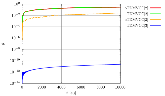
Figure 3: Hilbert space ket angles for water at the oTDMVCC[2–3] and TDMVCC[2–3] levels with $N=8$ and $N_{\mspace{-2.0mu}\mathrm{\scriptscriptstyle A}}=8$ for all modes. The angles are computed relative to tdfvci.

IV.1.2 acf

Figure 4(a) shows that oTDMVCC[3] and TDMVCC[3] are both visually converged with respect to the tdfvci reference, while oTDMVCC[2] and TDMVCC[2] exhibit a visible but rather modest error. Although oTDMVCC[3] produces visually converged acf, the absolute error (Fig. 4(b)) clearly shows that the tdfvci result is not exactly reproduced.

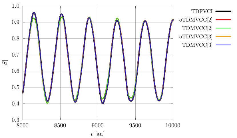
(a) Autocorrelation function

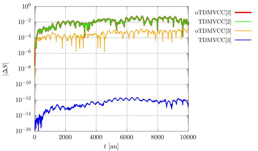
(b) Absolute error in autocorrelation function

Figure 4: ivr of water at the oTDMVCC[2–3] and TDMVCC[2–3] levels with $N=8$ and $N_{\mspace{-2.0mu}\mathrm{\scriptscriptstyle A}}=8$ for all modes. (a) acf. (b) Absolute error in the acf (relative to tdfvci).

IV.1.3 Expectation values

Figure 5 shows the expectation value of the displacement coordinates $Q_{0}$ (bend) and $Q_{1}$ (symmetric stretch). The remaining mode $Q_{2}$ (asymmetric stretch) is not shown since it couples only very weakly to $Q_{0}$ and $Q_{1}$ and is barely displaced during the simulation. Again, we observe that oTDMVCC[3] and TDMVCC[3] are visually identical to tdfvci. oTDMVCC[2] and TDMVCC[2] show small errors in $\langle Q_{1}\rangle$ (Fig. 5(b)) and somewhat larger errors in $\langle Q_{0}\rangle$, especially at later times. The absolute errors (Fig. 6) again demonstrate the non-convergence of the otdmvcc hierarchy.

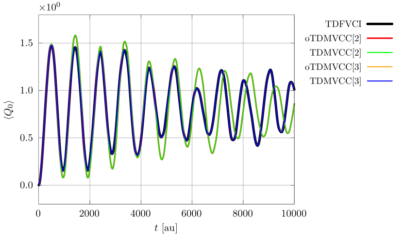
(a)

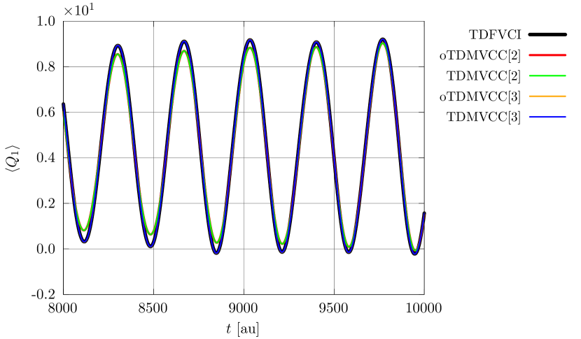
(b)

Figure 5: ivr of water at the oTDMVCC[2–3] and TDMVCC[2–3] levels with $N=8$ and $N_{\mspace{-2.0mu}\mathrm{\scriptscriptstyle A}}=8$ for all modes. (a) Expectation value of $Q_{0}$ (bend). (b) Expectation value of $Q_{1}$ (symmetric stretch).

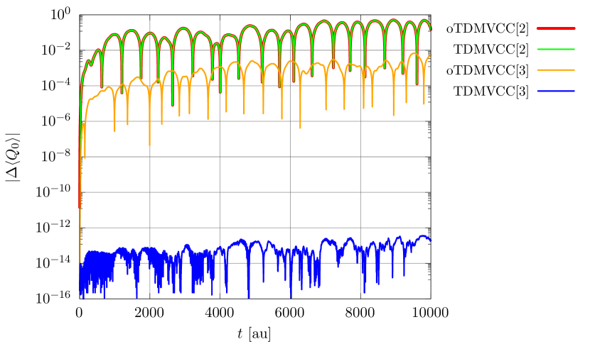
(a)

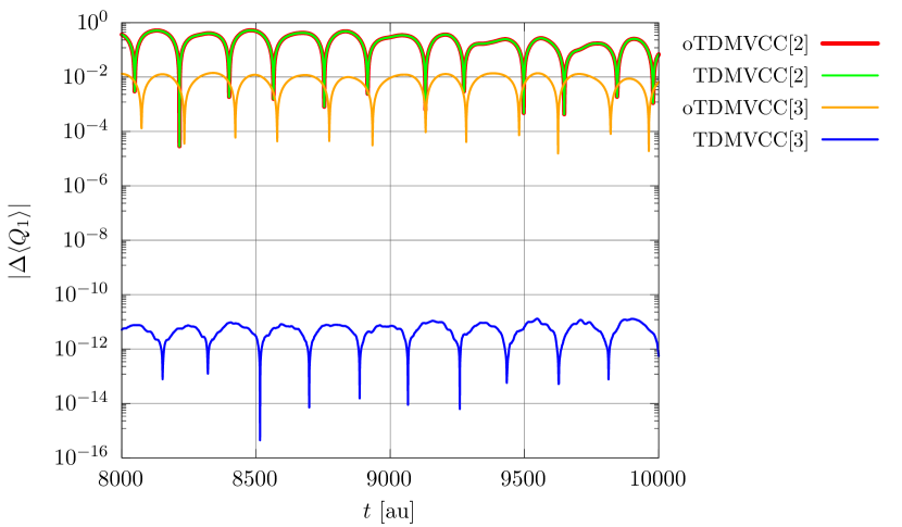
(b)

Figure 6: ivr of water at the oTDMVCC[2–3] and TDMVCC[2–3] levels with $N=8$ and $N_{\mspace{-2.0mu}\mathrm{\scriptscriptstyle A}}=8$ for all modes. (a) Absolute error in the expectation value of $Q_{0}$ (bend). (b) Absolute error in the expectation value of $Q_{1}$ (symmetric stretch).

IV.2 Ozone and sulfur dioxide

These molecules behave similarly to water in terms of convergence to tdfvci (the results can be found in the supplementary material). oTDMVCC[3] is always visually converged for sulfur dioxide, while small errors can sometimes be seen for ozone.

IV.3 Hydrogen sulfide

IV.3.1 acf

The hydrogen sulfide case is interesting because it stands out from the remaining triatomic molecules (water, ozone and sulfur dioxide). We note, for example, that the oTDMVCC[2] and TDMVCC[2] acf in Fig. 7 are quite far from the exact result. The prediction at the doubles level is in fact qualitatively wrong, which suggests that the validity of the cc ansatz is challenged. We remark that oTDMVCC[2] and TDMVCC[2] appear to be exactly equivalent, even in this seemingly difficult case. This surprising fact is discussed in more detail in Sec. IV.5.

oTDMVCC[3] restores qualitative agreement with tdfvci, but errors are still clearly visible. Only TDMVCC[3] succeeds in reproducing the correct result, which we see as an indication that the formal deficiency of the orthogonal formalism can have practical consequences.

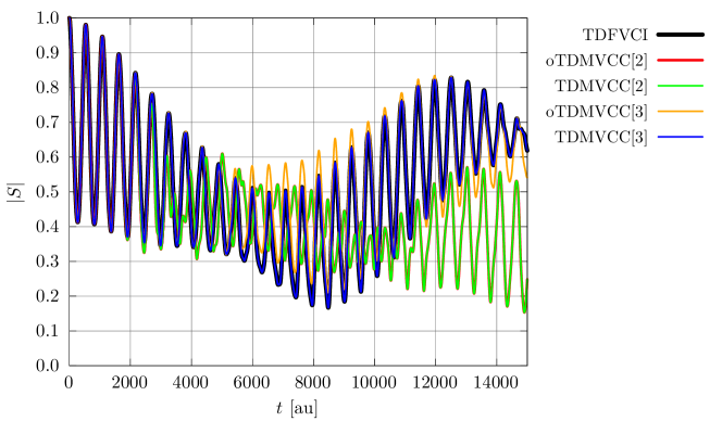
Figure 7: acf for the ivr of hydrogen sulfide at the oTDMVCC[2–3] and TDMVCC[2–3] levels with $N=8$ and $N_{\mspace{-2.0mu}\mathrm{\scriptscriptstyle A}}=8$ for all modes.

IV.3.2 Expectation values

For the $Q_{0}$ and $Q_{1}$ expectation values (Fig. 8), the picture is much the same as for the acf. The oTDMVCC[2]/TDMVCC[2] errors are rather large for $\langle Q_{0}\rangle$ (Fig. 8(a)), while the error in $\langle Q_{1}\rangle$ (Fig. 8(b)) is less striking. In the latter case, the overall shape of the curve is quite reasonable, but the period of the motion is not correct. oTDMVCC[3] agrees reasonably well with the tdfvci result, which could be takes as an indication that the wave function is in some sense well-behaved, in spite of the apparent error. However, Fig. 9 shows that $\mathrm{Im}\langle\Psi^{\prime}|Q|\Psi\rangle$ is in fact quite large compared to $\langle Q\rangle=\mathrm{Re}\langle\Psi^{\prime}|Q|\Psi\rangle$ for $Q_{0}$ and $Q_{1}$. Although a large imaginary part has no experimental meaning, we take it as yet another clear sign that the oTDMVCC wave function is generally not able to reproduce the exact wave function. We will only comment explicitly on the unphysical imaginary part for the hydrogen sulfide case, where it is largest. However, as shown in the supplementary material, we also find significant imaginary parts in otdmvcc calculations at full excitation level for some of the other molecules.

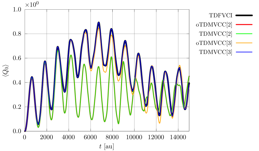
(a)

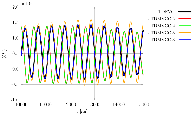
(b)

Figure 8: ivr of hydrogen sulfide at the oTDMVCC[2–3] and TDMVCC[2–3] levels with $N=8$ and $N_{\mspace{-2.0mu}\mathrm{\scriptscriptstyle A}}=8$ for all modes. (a) Expectation value of $Q_{0}$ (bend). (b) Expectation value of $Q_{1}$ (symmetric stretch).

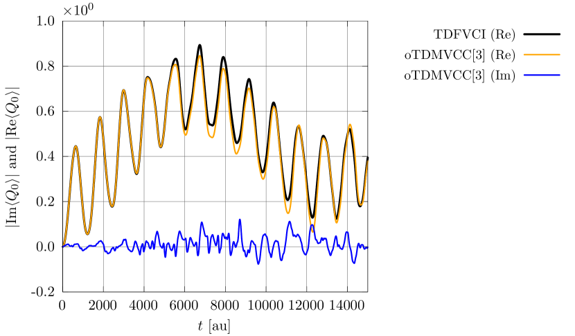
(a)

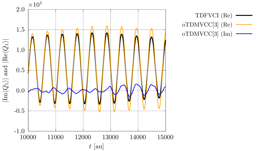
(b)

Figure 9: ivr of hydrogen sulfide at the oTDMVCC[3] level with $N=8$ and $N_{\mspace{-2.0mu}\mathrm{\scriptscriptstyle A}}=8$ for all modes. $\mathrm{Re}\langle\Psi^{\prime}|Q|\Psi\rangle$ and $\mathrm{Im}\langle\Psi^{\prime}|Q|\Psi\rangle$ for (a) $Q_{0}$ (bend) and (b) $Q_{1}$ (symmetric stretch).

IV.3.3 Amplitude norms

The fact that oTDMVCC[3] deviates visibly from TDMVCC[3] is reflected by the amplitude norms in Fig. 10 (the remaining triatomic molecules are also shown for comparison). We note the following: (i) For water and sulfur dioxide, the amplitude norms are small and there is good agreement between $T$ and $L$, and between oTDMVCC[3] and TDMVCC[3]; (ii) For ozone, the amplitudes are comparatively large and differ visibly; and (iii) For hydrogen sulfide, the amplitudes are again large and differ by a significant amount (the difference is particularly large between the TDMVCC[3] $T$ and $L$ amplitudes). At the same time, the TDMVCC[3] basis set shows considerable non-orthogonality in the hydrogen sulfide case (see Figs. S48–S50 in the supplementary material). We interpret this as a symptom that the cc ansatz is straining to describe the hydrogen sulfide dynamics correctly. The TDMVCC[3] is able to reproduce tdfvci (as it should), but only by using rather large amplitudes and the full flexibility of having a biorthogonal basis set. The oTDMVCC[3] ansatz is simply not sufficiently flexible in this particular case.

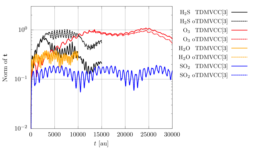
(a) $T$ amplitude norm

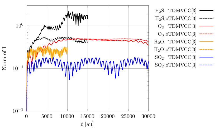
(b) $L$ amplitude norm

Figure 10: oTDMVCC[3] and TDMVCC[3] amplitude vector norms for the ivr of water, ozone, sulfur dioxide and hydrogen sulfide. Note that full and dotted lines may coincide.

IV.4 5D trans-bithiophene

IV.4.1 acf

For trans-bithiophene, the acf is almost visually converged already at the oTDMVCC[2] and TDMVCC[2] levels (Fig. 11(a)). The differences between the various levels only become visible when looking rather closely (Fig. 11(b)), and it is revealed that oTDMVCC[2] and TDMVCC[2] are very similar (though not quite identical), while showing a small error relative to the mctdh reference. TDMVCC[5] lies exactly on top of the mctdh trace, while the remaining calculations are very close to it. The precise ranking is given in terms of the average absolute error in Fig. 12. We note that the TDMVCC$[n]$ error is less than or equal to the oTDMVCC$[n]$ error for all $n$, and that the errors are always small.

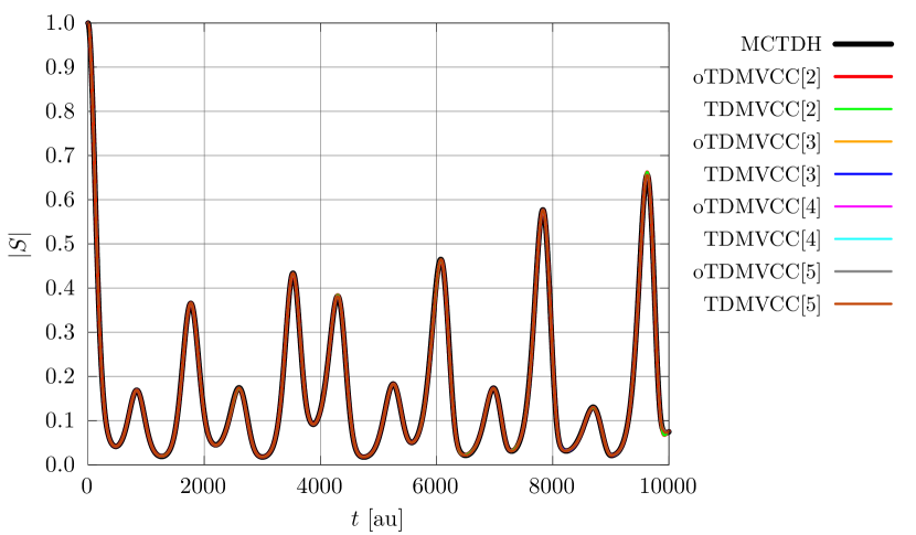
(a) Full time interval

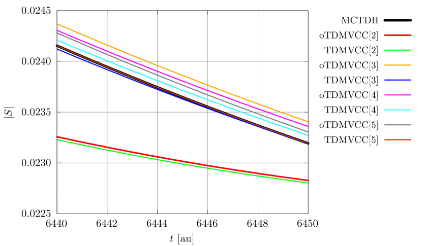
(b) Excerpt

Figure 11: acf for a 5D trans-bithiophene model at the oTDMVCC[2–5] and TDMVCC[2–5] levels with $N=30$ and $N_{\mspace{-2.0mu}\mathrm{\scriptscriptstyle A}}=4$ for all modes.

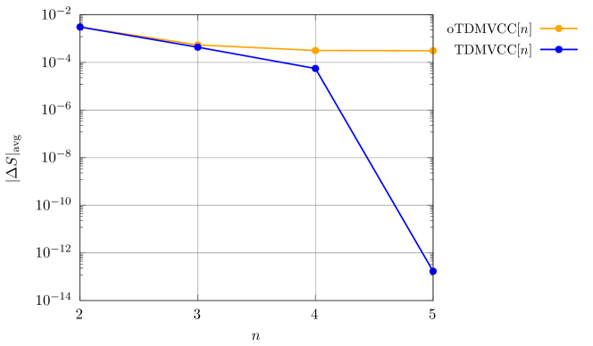
Figure 12: Average error in the acf for a 5D trans-bithiophene model at the oTDMVCC[2–5] and TDMVCC[2–5] levels with $N=30$ and $N_{\mspace{-2.0mu}\mathrm{\scriptscriptstyle A}}=4$ for all modes. The errors are computed relative to mctdh (the first $100\text{\,}\mathrm{a}\mathrm{u}$ have been excluded from the average).

IV.4.2 Expectation values

Figure 13 displays the expectation value $\langle Q_{10}\rangle$ and the absolute error relative to mctdh. The results all appear converged to the unaided eye (Fig. 13(a)), but the absolute error (Fig. 13(b)) shows that this is not exactly the case. It is clear that oTDMVCC[2]/TDMVCC[2] and oTDMVCC[3]/TDMVCC[3] yield pairwise near-identical values of $\langle Q_{10}\rangle$ and that TDMVCC[5] is fully converged. The relative quality of oTDMVCC[4], TDMVCC[4] and oTDMVCC[5] is not obvious from Fig. 13(b), but it is resolved quite clearly by Fig. 14: oTDMVCC[4] performs slightly better than both TDMVCC[4] and, surprisingly, oTDMVCC[5]. We note the strong oscillations in the absolute error (Fig. 13(b)) near $t=0$. These are caused by the singular initial density matrices (due to the vscf initial state), which make the eom somewhat difficult to integrate. We have thus chosen to exclude the first $100\text{\,}\mathrm{a}\mathrm{u}$ from the computation of the average shown in Fig. 14.

The expectation values for the remaining modes in the 5D model system are provided in the supplementary material (see Figs. S58–S65). These modes behave in much the same way as $Q_{10}$, also with respect to the ranking of the various levels of theory.

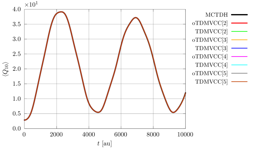
(a) Expectation value

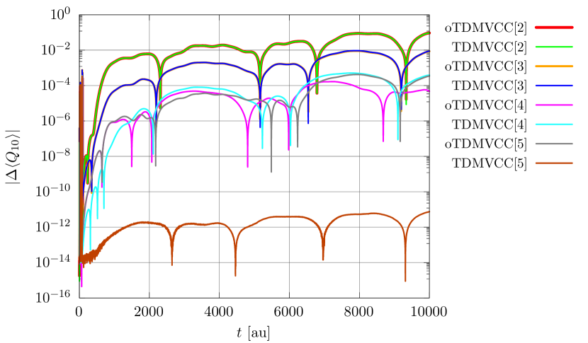
(b) Absolute error in expectation value

Figure 13: 5D trans-bithiophene model at the oTDMVCC[2–5] and TDMVCC[2–5] levels with $N=30$ and $N_{\mspace{-2.0mu}\mathrm{\scriptscriptstyle A}}=4$ for all modes. (a) Expectation value of $Q_{10}$. (b) Absolute error in the expectation value (relative to mctdh).

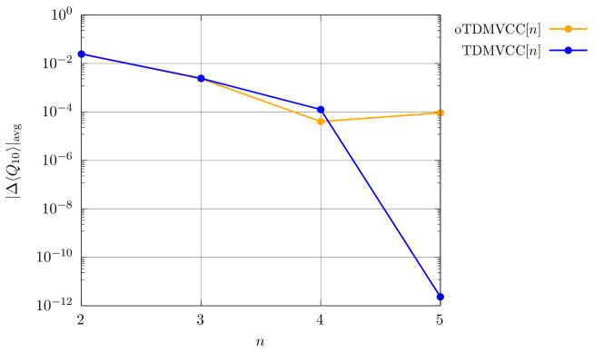
Figure 14: Average absolute error in the expectation value of $Q_{10}$ for a 5D trans-bithiophene model at the oTDMVCC[2–5] and TDMVCC[2–5] levels with $N=4$ and $N_{\mspace{-2.0mu}\mathrm{\scriptscriptstyle A}}=4$ for all modes. The errors are computed relative to mctdh (the first $100\text{\,}\mathrm{a}\mathrm{u}$ have been excluded from the average).

IV.5 Are oTDMVCC[2] and TDMVCC[2] equivalent?

For the triatomic molecules, our results show that oTDMVCC[2] are TDMVCC[2] are identical up to numerical precision (this is confirmed by inspecting the Hilbert space angles between the oTDMVCC[2] and TDMVCC[2] wave functions; see Fig. S51). It is not surprising that the two methods should yield similar predictions in many cases, but we find the agreement rather striking, in particular for the demanding case of hydrogen sulfide. Here, one might expect to see a clear manifestation of the difference between the orthogonal and biorthogonal formalisms, especially since such a difference is visible at the triples level.

We explain this surprising result with the following observations: First, we note that the oTDMVCC[2] and TDMVCC[2] expansions assume a very particular form for two- and three-mode systems:

$$\ket{\Psi} =e^{T}\ket{\Phi}$$

$$=e^{t_{0}}(1+T_{2})\ket{\Phi},$$ (103a)

$$\bra{\Psi^{\prime}} =\bra{\Phi^{\prime}}Le^{-T}$$

$$=\bra{\Phi^{\prime}}(l_{0}+L_{2})(1+T_{2})e^{-t_{0}}$$

$$=\bra{\Phi^{\prime}}\big{(}(l_{0}+L_{2}T_{2})+L_{2}\big{)}e^{-t_{0}}$$

$$\equiv\bra{\Phi^{\prime}}(l_{0}^{\prime}+L_{2})e^{-t_{0}}.$$ (103b)

This is essentially a CI-type expansion, although with a somewhat peculiar normalization. The second observation is that the vscf initial state has an orthogonal basis and satisfies $\bra{\Psi^{\prime}}=\ket{\Psi}^{\dagger}$. We thus have an initial state with symmetry between bra and ket, and a parameterization that allows this symmetry to be maintained. Numerically, we find that the one-mode density matrices stay Hermitian and that the mean fields satisfy $\check{\mathbf{F}}=\check{\mathbf{F}}^{\prime\dagger}$ for each mode (see Figs. S11, S22, S33 and S44). In essence, we get variational rather than bivariational time evolution for this special case. This also has the effect that expectation values like $\langle\Psi^{\prime}|Q|\Psi\rangle$ and $\langle\Psi^{\prime}|H|\Psi\rangle$ are strictly real, as can be seen in the supplementary material.

For trans-bithiophene, oTDMVCC[2] are TDMVCC[2] are very similar, and one must look closely (e.g. Fig 11(b)) to see a difference. It is of course difficult to define precisely what it means for two calculations to be strictly identical due to the presence of integration error and numerical noise. However, if we take the agreement between TDMVCC[5] and mctdh (Fig 11(b)) as a benchmark for perfect agreement, then it is clear that oTDMVCC[2] are TDMVCC[2] are not exactly identical. We are also not able to see any mathematical reason that the oTDMVCC[2] and TDMVCC[2] equations should generally be equivalent.

V Summary and outlook

The eom for bivariational wave functions with orthogonal, adaptive basis functions have been derived from a tdbvp. The use of an orthogonal basis makes the parameterization non-holomorphic (non-analytic in the complex sense), which necessitates the use of a manifestly real action functional in the derivations. We relate the orthogonal formalism (real action) to the corresponding biorthogonal formalism (complex action) in a transparent way and analyze similarities and differences. The general eom are then specialized to the cc ansatz and implemented for the nuclear dynamics problem. We denote the resulting method as otdmvcc (orthogonal tdmvcc) in order to distinguish it from tdmvcc, which uses a biorthogonal basis set. The otdmvcc amplitude equations are unchanged relative to the biorthogonal case, while the linear equations that determine the basis set time evolution (the so-called constraint equations) are symmetrized in a particular manner. Although the orthogonal and biorthogonal formalisms thus rely on the same matrix elements, the symmetrization has some consequences for the practical implementation of the constraint equations. In particular, the orthogonal formalism leads to constraint equations that couple all modes, in contrast to the biorthogonal constraint equations that can be solved one mode at a time. At the doubles level, certain simplification occur so that the oTDMVCC[2] constraint equations can also be solved mode by mode. The computational cost of oTDMVCC[2] is thus identical to that of TDMVCC[2]. At higher excitation levels, the orthogonal formalism generally involves a larger computational and implementation effort.

It is knownKöhn and Olsen (2005) that cc with orthogonal optimized or adaptive basis functions does not converge to the exact solution, even when the cluster expansion is complete. The precise convergence behavior is, however, not well understood, although electron dynamics studies by Sato and coworkersSato et al. (2018); Pathak, Sato, and Ishikawa (2020, 2021) indicate that no substantial error is introduced by using an orthogonal basis. We benchmarked all members of the oTDMVCC and TDMVCC hierarchies against tdfvci or mctdh for a number of triatomics (water, ozone, sulfur dioxide and hydrogen sulfide) and for a 5D model of the trans-bithiophene molecule. It is confirmed very clearly that TDMVCC converges to the exact limit, while oTDMVCC does not. For 5D trans-bithiophene, the oTDMVCC[5] observables are visually converged relative to the exact result, and differences are only revealed on close inspection. Water and sulfur dioxide behave similarly in the sense that the oTDMVCC[3] results appear fully converged to the unaided eye. For ozone, small errors are visible at the oTDMVCC[3] level, while hydrogen sulfide shows very clear differences between oTDMVCC[3] and TDMVCC[3]/TDFVCI (which are equivalent for a three-mode system). This difference correlates with rather large amplitudes, which indicates that the coupled cluster expansion is struggling in order to describe the wave function. In this difficult case, only TDMVCC[3] is able to reproduce TDFVCI due to the added flexibility of having a biorthogonal basis. Based on the examples at hand, our conclusion is thus that the orthogonal and biorthogonal formalisms agree quite closely in many cases, although noticeable differences are certainly possible.

We have emphasized two drawbacks of the oTDMVCC hierarchy, namely the lack of convergence to the exact limit and the fact that it involves larger sets of linear equations compared to the TDMVCC method. However, the TDMVCC method also has a drawback in the sense that it can sometimes be prone to numerical instability when the basis is split into and active and a secondary basis.Højlund et al. (2022) The so-called restricted polar scheme presented in Ref. 41 solves the stability problem without deteriorating accuracy, but the scheme is not fully bivariational. It is thus highly pertinent to investigate new formalisms that combine the following desirable properties in a fully bivariational way: (i) Numerical stability; (ii) convergence to the exact solution; and (iii) simple linear equations. Such a formalism is the subject of current research in our group.

Supplementary material

The supplementary material contains results for ozone and sulfur dioxide, as well as additional details for water, hydrogen sulfide and 5D trans-bithiophene.

Author declarations

Conflict of Interest

The authors have no conflicts to disclose.

Author Contributions

Mads Greisen Højlund: Conceptualization (equal); Data curation (lead); Formal analysis (equal); Investigation (lead); Software (lead); Visualization (lead); Writing – original draft (lead); Writing – review & editing (equal). Alberto Zoccante: Conceptualization (equal); Formal analysis (equal); Writing – review & editing (equal). Ove Christiansen: Conceptualization (equal); Formal analysis (equal); Funding acquisition (lead); Project administration (lead); Supervision (lead); Writing – review & editing (equal).

Data availability

The data that supports the findings of this study are available within the article and its supplementary material.

Appendix A Complex analysis

This appendix covers a few basic aspects of complex analysis. Our description is strongly inspired by Chapter 2.2 of Ref. 43 to which we refer the reader for further details. For simplicity of notation, we consider only functions of a single complex variable, e.g. $f:\Omega\rightarrow\mathbb{C}$, where the domain $\Omega$ is an open set in $\mathbb{C}$. We are free to write the function $f$ and its argument $z$ in terms of real and imaginary parts, i.e.

$$z=x+iy,$$ (A1)

$$f(z)=f(x,y)=u(x,y)+iv(x,y),$$ (A2)

where $x,y,u,v$ are real. As an entry point to our discussion, let us consider a common kind of problem, namely the problem of making $f$ stationary:

$$\partialderivative{f}{x}=0,\quad\partialderivative{f}{y}=0.$$ (A3)

Here, $\partial/\partial x$ and $\partial/\partial y$ denote partial derivatives in the ordinary, real sense. Separating $f$ into real and imaginary parts, this is obviously equivalent to

$$\partialderivative{u}{x}=0,\quad\partialderivative{v}{x}=0,\quad\partialderivative{u}{y}=0,\quad\partialderivative{v}{y}=0,$$ (A4)

which are four real equations with two real unknowns. Such a system cannot have a solution unless $f$ has some additional structure that eliminates two of the equations. We will discuss two kinds of structure that are relevant to our work, one which is mathematically trivial and one which has far-reaching consequences. The first case can be stated as

$$f(x,y)=\alpha+\beta g(x,y),$$ (A5)

where $g$ is a real-valued function and $\alpha,\beta$ are complex numbers. This includes $f$ being real, which is of course a common situation, or purely imaginary. Making $f$ stationary with respect to $x$ and $y$ is now a matter of solving two real equations with two real unknowns:

$$\partialderivative{g}{x}=0,\quad\partialderivative{g}{y}=0.$$ (A6)

A solution need not exist, of course, but we cannot rule out the possibility without more information.

In the second case, $f$ is holomorphic. The function $f$ is holomorphic (or complex differentiable) at the point $z_{0}\in\Omega$ if the quotient

$$\frac{f(z_{0}+h)-f(z_{0})}{h}$$ (A7)

converges to a limit when $h\rightarrow 0$. In that case, the limit is denoted by $f^{\prime}(z_{0})$, and is called the derivative of $f$ at $z_{0}$:

$$f^{\prime}(z_{0})=\lim_{h\rightarrow 0}\frac{f(z_{0}+h)-f(z_{0})}{h}.$$ (A8)

Although this definition looks exactly like the definition of a real derivative, it should be emphasized that $h$ is complex number that may approach $0$ from any direction. This turns out to have profound implications. A holomorphic function is, for example, infinitely differentiable, i.e. the existence of the first derivative guarantees the existence of all higher derivatives.Stein and Shakarchi (2003) Holomorphic functions are also analytic in the sense that they are given (locally) by a convergent power series expansion.Stein and Shakarchi (2003)

One can easily show (by taking $h$ to be real and then purely imaginary) that the existence of $f^{\prime}(z_{0})$ implies

$$f^{\prime}(z_{0})=\partialderivative{f}{x}\/(z_{0})=\frac{1}{i}\partialderivative{f}{y}\/(z_{0})$$ (A9)

or, after separating real and imaginary parts,

$$\partialderivative{u}{x}=\partialderivative{v}{y},\quad\partialderivative{u}{y}=-\partialderivative{v}{x}.$$ (A10)

These are the Cauchy-Riemann conditions, which connect real and complex analysis. We note that the Cauchy-Riemann conditions eliminate two equations in Eq. (A4), so that we are left with two real equations with two real unknowns. Equation (A9) also implies that

$$\partialderivative{f}{z}\/(z_{0}) \equiv\frac{1}{2}\left(\partialderivative{f}{x}\/(z_{0})+\frac{1}{i}\partialderivative{f}{y}\/(z_{0})\right) =f^{\prime}(z_{0}),$$ (A11)

$$\partialderivative{f}{z^{*}}\/(z_{0}) \equiv\frac{1}{2}\left(\partialderivative{f}{x}\/(z_{0})-\frac{1}{i}\partialderivative{f}{y}\/(z_{0})\right) =0,$$ (A12)

if $f$ is holomorphic. Here, we have defined the differential operators $\partial/\partial z$ and $\partial/\partial z^{*}$, which are sometimes called Wirtinger derivatives. These derivatives are, in principle, nothing more that a shorthand for a certain combination of real derivatives, but they are nonetheless very convenient. Equation (A11) means that $\partial/\partial z$ agrees with the complex partial derivative for holomorphic functions, while Eq. (A12) states that holomorphic functions have no formal dependence on $z^{*}$. For non-holomorphic functions (where the complex derivative does not exist), the Wirtinger derivatives still have meaning provided the real derivatives $\partial/\partial x$ and $\partial/\partial y$ exist. With the definition of Wirtinger derivatives, the optimization problem in Eq. (A3) is equivalent to

$$\partialderivative{f}{z}=0,\quad\partialderivative{f}{z^{*}}=0,$$ (A13)

where $z$ and $z^{*}$ are considered as independent variables. For a holomorphic function $f$, the latter equation is identically zero, and we are simply left with

$$\partialderivative{f}{z}=0.$$ (A14)

For a non-holomorphic function $f$, both equations must generally be considered.

Wirtinger derivatives have a number of pleasant properties that greatly simplify practical calculations:

$$\left(\partialderivative{f}{z}\right)^{\!*} =\partialderivative{f^{*}}{z^{*}}$$ (A15)

$$\left(\partialderivative{f}{z^{*}}\right)^{\!*} =\partialderivative{f^{*}}{z}$$ (A16)

$$\partialderivative{z}\/(fg) =\partialderivative{f}{z}g+f\partialderivative{g}{z}\quad$$ (product rule) (A17)

$$\partialderivative{z^{*}}\/(fg) =\partialderivative{f}{z^{*}}g+f\partialderivative{g}{z^{*}}\quad$$ (product rule) (A18)

$$\partialderivative{z}\/(f\circ g) =\left(\partialderivative{f}{z}\circ g\right)\partialderivative{g}{z}+\left(\partialderivative{f}{z^{*}}\circ g\right)\partialderivative{g^{*}}{z}\quad$$ (chain rule) (A19)

$$\partialderivative{z^{*}}\/(f\circ g) =\left(\partialderivative{f}{z}\circ g\right)\partialderivative{g}{z^{*}}+\left(\partialderivative{f}{z^{*}}\circ g\right)\partialderivative{g^{*}}{z^{*}}\quad$$ (chain rule) (A20)

$$\partialderivative{z}{z^{*}} =\partialderivative{z^{*}}{z} =0,$$ (A21)

$$\partialderivative{z}{z} =\partialderivative{z^{*}}{z^{*}} =1.$$ (A22)

The mechanics of computing Wirtinger derivatives is thus essentially identical to that of computing real derivatives, provided we think about $z$ and $z^{*}$ as independent variables. In addition, we never need to think about real and imaginary parts explicitly.

An important mapping that is not holomorphic is complex conjugation, $f(z)=z^{*}$. Indeed,

$$\frac{f(z_{0}+h)-f(z_{0})}{h}=\frac{h^{*}}{h},$$ (A23)

which has no limit as $h\rightarrow 0$. This is easily checked by taking $h$ to be real (in which case the quotient equals $1$) and then purely imaginary (in which case the quotient equals $-1$). Another common function is the square modulus, $f(z)=\absolutevalue{z}^{2}=zz^{*}$, which is non-holomorphic due to the presence of $z^{*}$. In spite of this, we can make $f$ stationary without resorting to real and imaginary parts by making use of the Wirtinger derivatives:

$$\partialderivative{f}{z}=z^{*}=0,\quad\partialderivative{f}{z^{*}}=z=0.$$ (A24)

The solution is obviously $z=0$. It is noted that since $f$ is real, the two equations are each other’s complex conjugate, so that one equation is effectively eliminated.

For non-holomorphic functions like Eq. (A5) we find that the optimization problem becomes

$$\partialderivative{f}{z}=\beta\partialderivative{g}{z}=0,\quad\partialderivative{f}{z^{*}}=\beta\partialderivative{g}{z^{*}}=0.$$ (A25)

or, equivalently,

$$\partialderivative{g}{z}=0,\quad\partialderivative{g}{z^{*}}=0.$$ (A26)

Since $g$ is real, the two equations are simply each other’s complex conjugate, so we only need to solve one of them.

For generic non-holomorphic functions we cannot hope for a solution. As an example, consider $f(z)=z^{2}+z^{*}$. Attempting to make this function stationary yields

$$\partialderivative{f}{z}=2z=0,\quad\partialderivative{f}{z^{*}}=1=0,$$ (A27)

which has no solution. This mirrors the discussion after Eq. (A4).

Appendix B Basis set eom

We can reuse the derivation of the complex Lagrangian $\mathcal{L}$ from Ref. 41 since the wave function does not depend on $\bm{\alpha}^{*}$. The modifications necessary to account for an orthonormal (rather than biorthonormal) basis are straight forward and the result reads

$$\mathcal{L} =\langle\Psi^{\prime}|(i\partial_{t}-H)|\Psi\rangle$$

$$=i\sum_{j}\dot{\alpha}_{j}m_{j}-\mathcal{H}^{\prime}$$ (B1)

where $m_{j}$ depends only on the configurational parameters:

$$m_{j}(\bm{\alpha})=\Big{\langle}\Psi^{\prime}\mspace{2.0mu}\Big{|}\mspace{1.5mu}\partialderivative{\Psi}{\alpha_{j}}\Big{\rangle}.$$ (B2)

The quantity $\mathcal{H}^{\prime}$ is a modified energy function defined as

$$\mathcal{H}^{\prime}(\bm{\alpha},\mathbf{V},\dot{\mathbf{V}},\mathbf{V}^{*})=\langle\Psi^{\prime}|(H-g)|\Psi\rangle=\mathcal{H}-\mathcal{G}.$$ (B3)

This function contains a proper energy function,

$$\mathcal{H}(\bm{\alpha},\mathbf{V},\mathbf{V}^{*})=\langle\Psi^{\prime}|H|\Psi\rangle,$$ (B4)

and a constraint function,

$$\mathcal{G}(\bm{\alpha},\dot{\mathbf{V}},\mathbf{V}^{*}) =\langle\Psi^{\prime}|g|\Psi\rangle$$ (B5a)

$$=\sum_{m}\sum_{p^{m}q^{m}}\rho^{m}_{\mspace{0.0mu}q^{m}p^{m}}g^{m}_{{p}^{m}{q}^{m}}$$ (B5b)

$$=i\sum_{m}\sum_{p^{m}q^{m}}\rho^{m}_{\mspace{0.0mu}q^{m}p^{m}}\Big{(}\sum_{\alpha^{m}}V^{m*}_{\mspace{-2.0mu}\alpha^{m}p^{m}}\dot{V}^{m}_{\mspace{-2.0mu}\alpha^{m}q^{m}}\Big{)}.$$ (B5c)

We have used Eqs. (19) and (18b) and defined a one-mode density matrix $\bm{\rho}^{m}$ with elements

$$\rho^{m}_{\mspace{0.0mu}q^{m}p^{m}}(\bm{\alpha})=\langle\Psi^{\prime}|\tilde{E}^{m}_{{p}^{m}{q}^{m}}|\Psi\rangle.$$ (B6)

Note the reversed indices. Having determined $\mathcal{L}$, we are ready to compute $\bar{\mathcal{L}}$ as

$$\bar{\mathcal{L}} =\tfrac{1}{2}(\mathcal{L}+\mathcal{L}^{*})$$

$$=\tfrac{i}{2}\sum_{j}(\dot{\alpha}_{j}m_{j}-\dot{\alpha}_{j}^{*}m_{j}^{*})-\tfrac{1}{2}(\mathcal{H}^{\prime}+\mathcal{H}^{\prime*})$$ (B7)

Using the real Lagrangian from Eq. (B), the basis set ele read

$$0 =\partialderivative{\bar{\mathcal{L}}}{V^{m}_{\mspace{-2.0mu}\alpha^{m}q^{m}}}-\derivative{t}\partialderivative{\bar{\mathcal{L}}}{\dot{V}^{m}_{\mspace{-2.0mu}\alpha^{m}q^{m}}}$$

$$=\frac{1}{2}\derivative{t}\partialderivative{(\mathcal{H}^{\prime}+\mathcal{H}^{\prime*})}{\dot{V}^{m}_{\mspace{-2.0mu}\alpha^{m}q^{m}}}-\frac{1}{2}\partialderivative{(\mathcal{H}^{\prime}+\mathcal{H}^{\prime*})}{V^{m}_{\mspace{-2.0mu}\alpha^{m}q^{m}}}.$$ (B8)

The four terms are easily computed using Eqs. (B3), (B4) and (B5c). One finds that

$$\derivative{t}\partialderivative{\mathcal{H}^{\prime}}{\dot{V}^{m}_{\mspace{-2.0mu}\alpha^{m}q^{m}}} =-i\derivative{t}\sum_{p^{m}}\rho^{m}_{\mspace{0.0mu}q^{m}p^{m}}V^{m*}_{\mspace{-2.0mu}\alpha^{m}p^{m}}$$

$$=-i\sum_{p^{m}}\big{(}\dot{\rho}^{m}_{\mspace{0.0mu}q^{m}p^{m}}V^{m*}_{\mspace{-2.0mu}\alpha^{m}p^{m}}+\rho^{m}_{\mspace{0.0mu}q^{m}p^{m}}\dot{V}^{m*}_{\mspace{-2.0mu}\alpha^{m}p^{m}}\big{)},$$ (B9)

$$\derivative{t}\partialderivative{\mathcal{H}^{\prime*}}{\dot{V}^{m}_{\mspace{-2.0mu}\alpha^{m}q^{m}}} =0,$$ (B10)

$$\partialderivative{\mathcal{H}^{\prime}}{V^{m}_{\mspace{-2.0mu}\alpha^{m}q^{m}}} =\partialderivative{\mathcal{H}}{V^{m}_{\mspace{-2.0mu}\alpha^{m}q^{m}}}$$

$$=\check{F}^{\prime m}_{{q}^{m}{\alpha}^{m}},$$ (B11)

$$\partialderivative{\mathcal{H}^{\prime*}}{V^{m}_{\mspace{-2.0mu}\alpha^{m}q^{m}}} =\bigg{(}\partialderivative{\mathcal{H}}{V^{m*}_{\mspace{-2.0mu}\alpha^{m}q^{m}}}\bigg{)}^{\!*}+i\sum_{p^{m}}\rho^{m*}_{\mspace{0.0mu}p^{m}q^{m}}\dot{V}^{m*}_{\mspace{-2.0mu}\alpha^{m}p^{m}}$$

$$=\check{F}^{m*}_{{\alpha}^{m}{q}^{m}}+i\sum_{p^{m}}\rho^{m*}_{\mspace{0.0mu}p^{m}q^{m}}\dot{V}^{m*}_{\mspace{-2.0mu}\alpha^{m}p^{m}}$$ (B12)

Equations (B) and (B) introduce the half-transformed mean-field matrices $\check{\mathbf{F}}^{\prime m}$ and $\check{\mathbf{F}}^{m}$ with elements

$$\check{F}^{\prime m}_{{q}^{m}{\alpha}^{m}} =\partialderivative{\mathcal{H}}{V^{m}_{\mspace{-2.0mu}\alpha^{m}q^{m}}} =\langle\Psi^{\prime}|[H,a^{m\mspace{-0.5mu}\raisebox{0.90417pt}{$\scriptstyle\dagger$}}_{\mspace{0.0mu}\alpha^{m}}]\tilde{a}^{m}_{\mspace{0.0mu}q^{m}}|\Psi\rangle,$$ (B13a)

$$\check{F}^{m}_{{\alpha}^{m}{q}^{m}}, =\partialderivative{\mathcal{H}}{V^{m*}_{\mspace{-2.0mu}\alpha^{m}q^{m}}} =\langle\Psi^{\prime}|\tilde{a}^{m\mspace{-0.5mu}\raisebox{0.90417pt}{$\scriptstyle\dagger$}}_{\mspace{0.0mu}q^{m}}[a^{m}_{\mspace{0.0mu}\alpha^{m}},H]|\Psi\rangle.$$ (B13b)

The concrete expressions in terms of commutators hold in the vibrational caseMadsen et al. (2020a) and in the electronic caseHøjlund et al. (2022) after removal of mode indices. The corresponding fully transformed mean-field matrices are given by

$$\tilde{\mathbf{F}}^{\prime m} =\check{\mathbf{F}}^{\prime m}\mathbf{V}^{m},$$ (B14a)

$$\tilde{\mathbf{F}}^{m} =\mathbf{V}^{m\dagger}\check{\mathbf{F}}^{m}$$ (B14b)

with elements

$$\tilde{F}^{\prime m}_{{q}^{m}{p}^{m}} =\langle\Psi^{\prime}|[H,\tilde{a}^{m\mspace{-0.5mu}\raisebox{0.90417pt}{$\scriptstyle\dagger$}}_{\mspace{0.0mu}p^{m}}]\tilde{a}^{m}_{\mspace{0.0mu}q^{m}}|\Psi\rangle,$$ (B15a)

$$\tilde{F}^{m}_{{q}^{m}{p}^{m}} =\langle\Psi^{\prime}|\tilde{a}^{m\mspace{-0.5mu}\raisebox{0.90417pt}{$\scriptstyle\dagger$}}_{\mspace{0.0mu}p^{m}}[\tilde{a}^{m}_{\mspace{0.0mu}q^{m}},H]|\Psi\rangle.$$ (B15b)

The ele can now be written in matrix notation as

$$\mathbf{0} =-\frac{1}{2}\big{(}\check{\mathbf{F}}^{\prime m}+\check{\mathbf{F}}^{m\dagger}\big{)}-i\mathbb{H}[\bm{\rho}^{m}]\dot{\mathbf{V}}^{m\dagger}-\frac{i}{2}\dot{\bm{\rho}}^{m}\mathbf{V}^{m\dagger}$$ (B16)

where $\mathbb{H}[\,\cdot\,]$ denotes the Hermitian part of a square matrix. Multiplication of Eq. (B16) by $\mathbf{V}^{m}$ from the right then yields

$$\mathbf{0} =-\frac{1}{2}\big{(}\tilde{\mathbf{F}}^{\prime m}+\tilde{\mathbf{F}}^{m\dagger}\big{)}+\mathbb{H}[\bm{\rho}^{m}]\mathbf{G}^{m}-\frac{i}{2}\dot{\bm{\rho}}^{m}$$ (B17)

where we have used the unitarity of $\mathbf{V}^{m}$ as well as Eqs. (18a) and (B14). In order to proceed, we subtract Eq. (B17) from the Hermitian conjugate of Eq. (B17):

$$\mathbf{0} =\mathbb{A}(\mathbf{F}^{m})-\big{(}\mathbb{H}[\bm{\rho}^{m}]\mathbf{G}^{m}-\mathbf{G}^{m}\mathbb{H}[\bm{\rho}^{m}]\big{)}+i\mathbb{H}[\dot{\bm{\rho}}^{m}],$$

$$=\mathbb{A}\Big{[}\mathbf{F}^{m}-\big{(}\bm{\rho}^{m}\mathbf{G}^{m}-\mathbf{G}^{m}\bm{\rho}^{m}\big{)}+i\dot{\bm{\rho}}^{m}\Big{]}.$$ (B18)

Here, $\mathbb{A}$ denotes the anti-Hermitian part of a square matrix. The matrix $\mathbf{F}^{m}$ is defined as

$$\mathbf{F}^{m}=\tilde{\mathbf{F}}^{\prime m}-\tilde{\mathbf{F}}^{m}$$ (B19)

and has the elements

$$F^{m}_{{q}^{m}{p}^{m}}=\langle\Psi^{\prime}|[H,\tilde{E}^{m}_{{p}^{m}{q}^{m}}]|\Psi\rangle.$$ (B20)

Appendix C Simplification of Eq. (54c)

The element-wise form of Eq. (54c) reads

$$\frac{1}{2}\sum_{m^{\prime}}\sum_{y^{m^{\prime}}u^{m^{\prime}}}\Big{[}C_{({m}\,{t}^{m}{x}^{m})({m^{\prime}}{y}^{m^{\smash{\prime}}}\!{u}^{m^{\smash{\prime}}})}-C_{({m}\,{x}^{m}{t}^{m})({m^{\prime}}{u}^{m^{\smash{\prime}}}\!{y}^{m^{\smash{\prime}}})}^{*}\Big{]}g^{m^{\prime}}_{{y}^{m^{\smash{\prime}}}\!{u}^{m^{\smash{\prime}}}}\\ =\frac{1}{2}\Big{[}\langle\Psi^{\prime}|[H,\tilde{E}^{m}_{{t}^{m}{x}^{m}}]|\Psi\rangle-\langle\Psi^{\prime}|[H,\tilde{E}^{m}_{{x}^{m}{t}^{m}}]|\Psi\rangle^{*}\Big{]}.$$ (C1)

This left-hand side is simplified using Eqs. (30), while the right-hand side is re-written by expanding the commutators and using the killer conditions:

$$-\frac{1}{2}\sum_{m^{\prime}}\sum_{y^{m^{\prime}}u^{m^{\prime}}}\delta_{mm^{\prime}}\delta_{x^{m}y^{m}}\big{(}\rho^{m}_{\mspace{0.0mu}u^{m}t^{m}}+\rho^{m*}_{\mspace{0.0mu}t^{m}u^{m}}\big{)}g^{m^{\prime}}_{{y}^{m^{\smash{\prime}}}\!{u}^{m^{\smash{\prime}}}}\\ \begin{aligned} &=\begin{multlined}\frac{1}{2}\Big{[}\langle\Psi^{\prime}|[H,\tilde{a}^{m\mspace{-0.5mu}\raisebox{0.90417pt}{$\scriptstyle\dagger$}}_{\mspace{0.0mu}t^{m}}]\tilde{a}^{m}_{\mspace{0.0mu}x^{m}}|\Psi\rangle-\langle\Psi^{\prime}|\tilde{a}^{m\mspace{-0.5mu}\raisebox{0.90417pt}{$\scriptstyle\dagger$}}_{\mspace{0.0mu}t^{m}}[\tilde{a}^{m}_{\mspace{0.0mu}x^{m}},H]|\Psi\rangle\\ -\langle\Psi^{\prime}|[H,\tilde{a}^{m\mspace{-0.5mu}\raisebox{0.90417pt}{$\scriptstyle\dagger$}}_{\mspace{0.0mu}x^{m}}]\tilde{a}^{m}_{\mspace{0.0mu}t^{m}}|\Psi\rangle^{*}+\langle\Psi^{\prime}|\tilde{a}^{m\mspace{-0.5mu}\raisebox{0.90417pt}{$\scriptstyle\dagger$}}_{\mspace{0.0mu}x^{m}}[\tilde{a}^{m}_{\mspace{0.0mu}t^{m}},H]|\Psi\rangle^{*}\Big{]}\end{multlined}\frac{1}{2}\Big{[}\langle\Psi^{\prime}|[H,\tilde{a}^{m\mspace{-0.5mu}\raisebox{0.90417pt}{$\scriptstyle\dagger$}}_{\mspace{0.0mu}t^{m}}]\tilde{a}^{m}_{\mspace{0.0mu}x^{m}}|\Psi\rangle-\langle\Psi^{\prime}|\tilde{a}^{m\mspace{-0.5mu}\raisebox{0.90417pt}{$\scriptstyle\dagger$}}_{\mspace{0.0mu}t^{m}}[\tilde{a}^{m}_{\mspace{0.0mu}x^{m}},H]|\Psi\rangle\\ -\langle\Psi^{\prime}|[H,\tilde{a}^{m\mspace{-0.5mu}\raisebox{0.90417pt}{$\scriptstyle\dagger$}}_{\mspace{0.0mu}x^{m}}]\tilde{a}^{m}_{\mspace{0.0mu}t^{m}}|\Psi\rangle^{*}+\langle\Psi^{\prime}|\tilde{a}^{m\mspace{-0.5mu}\raisebox{0.90417pt}{$\scriptstyle\dagger$}}_{\mspace{0.0mu}x^{m}}[\tilde{a}^{m}_{\mspace{0.0mu}t^{m}},H]|\Psi\rangle^{*}\Big{]}\\ &=-\frac{1}{2}\Big{[}\langle\Psi^{\prime}|\tilde{a}^{m\mspace{-0.5mu}\raisebox{0.90417pt}{$\scriptstyle\dagger$}}_{\mspace{0.0mu}t^{m}}[\tilde{a}^{m}_{\mspace{0.0mu}x^{m}},H]|\Psi\rangle+\langle\Psi^{\prime}|[H,\tilde{a}^{m\mspace{-0.5mu}\raisebox{0.90417pt}{$\scriptstyle\dagger$}}_{\mspace{0.0mu}x^{m}}]\tilde{a}^{m}_{\mspace{0.0mu}t^{m}}|\Psi\rangle^{*}\Big{]}\end{aligned}$$ (C2)

Reducing the sums and introducing the mean-field matrices from Eqs. (28) now yields

$${{}^{t}\mathbf{G}^{m}}\;\mathbb{H}[{{}^{a\!}}\bm{{\mathchoice{\raisebox{1.0pt}{$\displaystyle\rho$}}{\raisebox{1.0pt}{$\textstyle\rho$}}{\raisebox{1.0pt}{$\scriptstyle\rho$}}{\raisebox{1.0pt}{$\scriptscriptstyle\rho$}}}}^{m}] =\tfrac{1}{2}({{}^{t}\tilde{\mathbf{F}}^{m}}+{{}^{b}\tilde{\mathbf{F}}^{\prime m\dagger}})$$ (C3a)

$$=\tfrac{1}{2}\mathbf{V}^{m\dagger}_{\!\!\mathrm{\scriptscriptstyle S}}(\check{\mathbf{F}}^{m}_{\!\!\mathrm{\scriptscriptstyle A}}+\check{\mathbf{F}}^{\prime m\dagger}_{\!\!\mathrm{\scriptscriptstyle A}}).$$ (C3b)

The latter expression follows directly from Eq. (B14).

Appendix D Constraint equations in electronic coupled cluster theory

The electronic structure equivalents of Eqs. (II.4), (91) and (92) are obtained by substituting $i^{m}\rightarrow i$ and $i^{m^{\prime}}\rightarrow j$ and then deleting all remaining mode indices:

$${{}^{ud}\bar{C}_{(ai)(jb)}} =\frac{1}{2}\Big{(}\langle\Psi^{\prime}|[\tilde{E}_{jb},\tilde{E}_{ai}]|\Psi\rangle-\langle\Psi^{\prime}|[\tilde{E}_{bj},\tilde{E}_{ia}]|\Psi\rangle^{*}\Big{)}$$

$$=\delta_{ab}\mathbb{H}[\bm{{\mathchoice{\raisebox{1.0pt}{$\displaystyle\rho$}}{\raisebox{1.0pt}{$\textstyle\rho$}}{\raisebox{1.0pt}{$\scriptstyle\rho$}}{\raisebox{1.0pt}{$\scriptscriptstyle\rho$}}}}]_{ij}-\delta_{ij}\mathbb{H}[\bm{{\mathchoice{\raisebox{1.0pt}{$\displaystyle\rho$}}{\raisebox{1.0pt}{$\textstyle\rho$}}{\raisebox{1.0pt}{$\scriptstyle\rho$}}{\raisebox{1.0pt}{$\scriptscriptstyle\rho$}}}}]_{ba}$$ (D1)

$${{}^{dd}\bar{C}^{\prime}_{(ia)(jb)}} =\frac{1}{2}\sum_{\mu}\Big{(}\langle\Psi|[\tilde{E}_{ia},\tau_{\mu}]|\Psi\rangle\langle\mu|e^{-T}\tilde{E}_{jb}|\Psi\rangle-\langle\Psi|[\tilde{E}_{jb},\tau_{\mu}]|\Psi\rangle\langle\mu|e^{-T}\tilde{E}_{ia}|\Psi\rangle\Big{)},$$ (D2)

$${{}^{d}\bar{f}^{\prime}_{(ia)}}=\frac{1}{2}\Big{(}\langle\Psi^{\prime}|[H,\tilde{E}_{ia}]|\Psi\rangle-\langle\Psi^{\prime}|[H,\tilde{E}_{ai}]|\Psi\rangle^{*}\Big{)}\\ \begin{aligned} t]{2}{}+\frac{1}{2}\sum_{\mu}\Big{(}\langle\Psi|[\tilde{E}_{ia},\tau_{\mu}]|\Psi\rangle\langle\mu|e^{-T}H|\Psi\rangle-\langle\Psi|[H,\tau_{\mu}]|\Psi\rangle\langle\mu|e^{-T}\tilde{E}_{ia}|\Psi\rangle\Big{)}.\end{aligned}$$ (D3)

References

- Madsen et al. (2020a) N. K. Madsen, M. B. Hansen, O. Christiansen, and A. Zoccante, J. Chem. Phys. 153, 174108 (2020a).
- Chiles and Dykstra (1981) R. A. Chiles and C. E. Dykstra, J. Chem. Phys. 74, 4544 (1981).
- Handy et al. (1989) N. C. Handy, J. A. Pople, M. Head-Gordon, K. Raghavachari, and G. W. Trucks, Chem. Phys. Lett. 164, 185 (1989).
- Raghavachari et al. (1990) K. Raghavachari, J. A. Pople, E. S. Replogle, M. Head-Gordon, and N. C. Handy, Chem. Phys. Lett. 167, 115 (1990).
- Hampel, Peterson, and Werner (1992) C. Hampel, K. A. Peterson, and H.-J. Werner, Chem. Phys. Lett. 190, 1 (1992).
- Stanton, Gauss, and Bartlett (1992) J. F. Stanton, J. Gauss, and R. J. Bartlett, J. Chem. Phys. 97, 5554 (1992).
- Barnes and Lindh (1994) L. A. Barnes and R. Lindh, Chem. Phys. Lett. 223, 207 (1994).
- Xie et al. (1996) Y. Xie, W. D. Allen, Y. Yamaguchi, and H. F. Schaefer, J. Chem. Phys. 104, 7615 (1996).
- Crawford and Stanton (2000) T. D. Crawford and J. F. Stanton, J. Chem. Phys. 112, 7873 (2000).
- Aiga, Sasagane, and Itoh (1994) F. Aiga, K. Sasagane, and R. Itoh, Int. J. Quantum Chem. 51, 87 (1994).
- Koch, Kobayashi, and Jørgensen (1994) H. Koch, R. Kobayashi, and P. Jørgensen, Int. J. Quantum Chem. 49, 835 (1994).
- Purvis and Bartlett (1982) G. D. Purvis and R. J. Bartlett, J. Chem. Phys. 76, 1910 (1982).
- Scuseria and Schaefer (1987) G. E. Scuseria and H. F. Schaefer, Chem. Phys. Lett. 142, 354 (1987).
- Sherrill et al. (1998) C. D. Sherrill, A. I. Krylov, E. F. C. Byrd, and M. Head-Gordon, J. Chem. Phys. 109, 4171 (1998).
- Krylov et al. (1998) A. I. Krylov, C. D. Sherrill, E. F. C. Byrd, and M. Head-Gordon, J. Chem. Phys. 109, 10669 (1998).
- Pedersen, Koch, and Hättig (1999) T. B. Pedersen, H. Koch, and C. Hättig, J. Chem. Phys. 110, 8318 (1999).
- Köhn and Olsen (2005) A. Köhn and J. Olsen, J. Chem. Phys. 122, 084116 (2005).
- Pedersen, Fernández, and Koch (2001) T. B. Pedersen, B. Fernández, and H. Koch, J. Chem. Phys. 114, 6983 (2001).
- Myhre (2018) R. H. Myhre, J. Chem. Phys. 148, 094110 (2018).
- Meyer, Manthe, and Cederbaum (1990) H.-D. Meyer, U. Manthe, and L. S. Cederbaum, Chem. Phys. Lett. 165, 73 (1990).
- Beck et al. (2000) M. H. Beck, A. Jäckle, G. A. Worth, and H.-D. Meyer, Phys. Rep. 324, 1 (2000).
- Zanghellini et al. (2003) J. Zanghellini, M. Kitzler-Zeiler, C. Fabian, T. Brabec, and A. Scrinzi, Laser Phys. 13, 1064 (2003).
- Kato and Kono (2004) T. Kato and H. Kono, Chem. Phys. Lett. 392, 533 (2004).
- Nest, Klamroth, and Saalfrank (2005) M. Nest, T. Klamroth, and P. Saalfrank, J. Chem. Phys. 122, 124102 (2005).
- Caillat et al. (2005) J. Caillat, J. Zanghellini, M. Kitzler, O. Koch, W. Kreuzer, and A. Scrinzi, Phys. Rev. A 71, 012712 (2005).
- Hansen et al. (2019) M. B. Hansen, N. K. Madsen, A. Zoccante, and O. Christiansen, J. Chem. Phys. 151, 154116 (2019).
- Hansen, Madsen, and Christiansen (2020) M. B. Hansen, N. K. Madsen, and O. Christiansen, J. Chem. Phys. 153, 044133 (2020).
- Madsen et al. (2020b) N. K. Madsen, A. B. Jensen, M. B. Hansen, and O. Christiansen, J. Chem. Phys. 153, 234109 (2020b).
- Schönhammer and Gunnarsson (1978) K. Schönhammer and O. Gunnarsson, Phys. Rev. B 18, 6606 (1978).
- Huber and Klamroth (2011) C. Huber and T. Klamroth, J. Chem. Phys. 134, 054113 (2011).
- Pedersen and Kvaal (2019) T. B. Pedersen and S. Kvaal, J. Chem. Phys. 150, 144106 (2019).
- Skeidsvoll, Balbi, and Koch (2020) A. S. Skeidsvoll, A. Balbi, and H. Koch, Phys. Rev. A 102, 023115 (2020).
- Hoodbhoy and Negele (1978) P. Hoodbhoy and J. W. Negele, Phys. Rev. C 18, 2380 (1978).
- Hoodbhoy and Negele (1979) P. Hoodbhoy and J. W. Negele, Phys. Rev. C 19, 1971 (1979).
- Pigg et al. (2012) D. A. Pigg, G. Hagen, H. Nam, and T. Papenbrock, Phys. Rev. C 86, 014308 (2012).
- Sverdrup Ofstad et al. (2023) B. Sverdrup Ofstad, E. Aurbakken, Ø. Sigmundson Schøyen, H. E. Kristiansen, S. Kvaal, and T. B. Pedersen, WIREs Comput. Mol. Sci. 13, e1666 (2023).
- Kvaal (2012) S. Kvaal, J. Chem. Phys. 136, 194109 (2012).
- Sato et al. (2018) T. Sato, H. Pathak, Y. Orimo, and K. L. Ishikawa, J. Chem. Phys. 148, 051101 (2018).
- Pathak, Sato, and Ishikawa (2020) H. Pathak, T. Sato, and K. L. Ishikawa, J. Chem. Phys. 152, 124115 (2020).
- Pathak, Sato, and Ishikawa (2021) H. Pathak, T. Sato, and K. L. Ishikawa, J. Chem. Phys. 154, 234104 (2021).
- Højlund et al. (2022) M. G. Højlund, A. B. Jensen, A. Zoccante, and O. Christiansen, J. Chem. Phys. 157, 234104 (2022).
- Arponen (1983) J. Arponen, Ann. Phys. 151, 311 (1983).
- Stein and Shakarchi (2003) E. M. Stein and R. Shakarchi, Complex Analysis, Princeton Lectures in Analysis No. 2 (Princeton University Press, Princeton, N.J, 2003).
- Pedersen and Koch (1997) T. B. Pedersen and H. Koch, J. Chem. Phys. 106, 8059 (1997).
- Pedersen and Koch (1998) T. B. Pedersen and H. Koch, J. Chem. Phys. 108, 12 (1998).
- Kristiansen et al. (2022) H. E. Kristiansen, B. S. Ofstad, E. Hauge, E. Aurbakken, Ø. S. Schøyen, S. Kvaal, and T. B. Pedersen, J. Chem. Theory Comput. 18, 3687 (2022).
- Christiansen (2004) O. Christiansen, J. Chem. Phys. 120, 2140 (2004).
- Helgaker, Jørgensen, and Olsen (2000) T. Helgaker, P. Jørgensen, and J. Olsen, Molecular Electronic-Structure Theory (Wiley, Chichester ; New York, 2000).
- Dirac (1950) P. A. M. Dirac, Can. J. Math. 2, 129 (1950).
- Ohta (2000) K. Ohta, Chem. Phys. Lett. 329, 248 (2000).
- Ohta (2004) K. Ohta, Phys. Rev. A 70, 022503 (2004).
- Christiansen et al. (2023) O. Christiansen, D. G. Artiukhin, F. Bader, I. H. Godtliebsen, E. M. Gras, W. Győrffy, M. B. Hansen, M. B. Hansen, M. G. Højlund, N. M. Høyer, R. B. Jensen, A. B. Jensen, E. L. Klinting, J. Kongsted, C. König, D. Madsen, N. K. Madsen, K. Monrad, G. Schmitz, P. Seidler, K. Sneskov, M. Sparta, B. Thomsen, D. Toffoli, and Alberto Zoccante, “MidasCpp,” (2023).
- Jensen et al. (2023) A. B. Jensen, M. G. Højlund, A. Zoccante, N. K. Madsen, and O. Christiansen, “Efficient time-dependent vibrational coupled cluster computations with time-dependent basis sets at the two-mode coupling level: Full and hybrid TDMVCC[2],” (2023), arxiv:2308.15245 [submitted to J. Chem. Phys.] .
- Højlund, Zoccante, and Christiansen (2023) M. G. Højlund, A. Zoccante, and O. Christiansen, J. Chem. Phys. 158, 204104 (2023).
- Majland et al. (2023) M. Majland, R. Berg Jensen, M. Greisen Højlund, N. Thomas Zinner, and O. Christiansen, Chem. Sci. 14, 7733 (2023).
- Madsen et al. (2019) D. Madsen, O. Christiansen, P. Norman, and C. König, Phys. Chem. Chem. Phys. 21, 17410 (2019).
- Hairer, Nørsett, and Wanner (2009) E. Hairer, S. P. Nørsett, and G. Wanner, Solving Ordinary Differential Equations I: Nonstiff Problems, 2nd ed., Springer Series in Computational Mathematics No. 8 (Springer, Heidelberg ; London, 2009).