Emergence of odd elasticity in a microswimmer using deep reinforcement learning

Abstract

We investigate the emergence of odd elasticity in an elastic microswimmer model by using Deep Q-Network with a reinforcement learning method. Although the swimming velocity decreases for an elastic microswimmer with prescribed dynamics in the large-frequency regime, the fully trained elastic microswimmer adapts a waiting strategy to avoid the velocity decrease. For the trained microswimmers, we evaluate the performance of the cycles by the product of the loop area (called non-reciprocality) and the loop frequency, and show that the average swimming velocity is proportional to the performance. By calculating the force-displacement correlations, we obtain the effective odd elasticity of the microswimmer to characterize its non-reciprocal dynamics. The emergent odd elasticity is closely related to the loop frequency of the cyclic deformation. The present work provides us with a clue to reveal the emergence of various non-reciprocal phenomena in active systems by using machine learning.

I Introduction

Active systems composed of self-driven units play a crucial role in biological processes as they are able to convert microscopic energy into macroscopic work Marchetti2013HydrodynamicsMatter ; Roadmap20 ; Shanker22 . To achieve sustainable work at the microscopic scale, active units must go through non-reciprocal cyclic motions Dey19 ; HK22 . For example, cyclic state transitions of enzymatic molecules are driven by catalytic chemical reactions Dey16 ; Aviram18 , which can be described by simple coarse-grained models Echeverria11 ; Mikhailov15 ; Hosaka20 . To evaluate the functionality of an enzyme, we previously defined a physical quantity called non-reciprocality that represents the area enclosed by a trajectory in the conformational space Yasuda21-a ; Kobayashi23b . According to Purcell’s scallop theorem for microswimmers moving in a viscous fluid Purcell77 ; Lauga09a ; Laugabook , the average swimming velocity is proportional to the non-reciprocality and the loop frequency of the cyclic body motion as long as the deformation is small. It was also reported that the crawling speed of a cell on a substrate is determined by the non-reciprocality Leoni15 ; Lenoi17 ; Tarama18 .

Recently, Scheibner et al. introduced the concept of odd elasticity that is useful to characterize non-equilibrium active systems Scheibner2020OddElasticity ; Fruchar2023 . Odd elasticity arises from antisymmetric (odd) components of the elastic modulus tensor violating the energy conservation law, and it can exist in active materials braverman2021 ; bililign21 ; surowka2022 ; Fossati23 , biological systems Tan22 , and active robots Ishimoto22 ; Ishimoto23 ; Coulais2021 . We emphasize here that the concept of odd elasticity is not limited to elastic materials but can be extended to various dynamical systems Yasuda22-machlup ; Yasuda22 . One useful example is a microswimmer with odd elasticity that can exhibit a directional locomotion in the presence of thermal agitations Yasuda21 . In fact, the average velocity of an odd microswimmer is proportional to the odd elasticity. In the model of a stochastic enzyme, on the other hand, we have quantified the average work per cycle in terms of effective odd elasticity Kobayashi23b . Hence, odd elasticity is a crucial quantity to characterize non-equilibrium micromachines such as proteins, enzymes, microswimmers, and robots.

Despite the importance of odd elasticity in active systems, its physical origin still needs to be better understood Mitarai02 . One possibility is to use Onsager’s variational principle DoiSoftMatterPhysics to derive dynamical equations for an active system with odd elasticity Lin23 . The obtained non-reciprocal equations Fruchart2021 manifest the physical origin of the odd elastic constant that is proportional to the non-equilibrium driving force Lin23 . On the other hand, odd elasticity may not be innate to micromachines, but can be an ability acquired after many experiences and training processes. In this work, considering an elastic three-sphere microswimmer model Pande15 ; Pande17 ; Yasuda17c , we utilize machine learning techniques to account for the emergence of odd elasticity. With this approach, a microswimmer can automatically obtain the most efficient swimming strategy without prescribing any deformation dynamics.

In recent years, machine learning has been widely applied to active systems as a powerful tool to unravel the complexities of biological systems cichos2020 ; stark2021 ; hartl2021 ; stark2023 . Notably, the application of reinforcement learning techniques are capable and versatile in training various microswimmers. These methods have been used to navigate them through complex and dynamical environments with remarkable adaptability, such as path-planning in turbulent flows or noisy surroundings schneider2019 ; alageshan2020 ; landin2021 ; nasiri2023 . Furthermore, machine learning has been applied to optimize the local motion and intricate navigation of microswimmers with complex structures or higher degrees of freedom tsang2020 ; zou2022 ; qin2023 . These approaches have been further extended to more difficult tasks, such as cooperative swimming and predation models borra2022 ; zhu2022 ; liu2023 .

The main aim of this paper is to reveal the emergence of odd elasticity in an elastic microswimmer model by using Deep Q-Network with reinforcement learning method. Although the swimming velocity decreases for an elastic microswimmer model with prescribed dynamics in the large-frequency regime Yasuda17c , the fully trained microswimmer in the current work adapts a waiting strategy to avoid the velocity decrease. From the obtained numerical data, we quantify the performance and effective odd elasticity of the trained microswimmer. The estimated cycle performance, which is the product of the non-reciprocality (loop area) and the loop frequency, coincides well with the swimming velocity by using a proper scale factor. We also demonstrate that the emergent odd elasticity of the microswimmer is closely related to the loop frequency of the cyclic deformation. The present work provides us with a clue to reveal the emergence of various non-reciprocal phenomena in active systems by using machine learning.

In Sec. II, we review the model of an elastic microswimmer with prescribed dynamics Yasuda17c . In Sec. III, we explain the deep reinforcement learning technique to train the elastic microswimmer. In Sec. IV, we describe the physical properties of the fully trained microswimmer. In particular, we shall discuss the emergence of limit cycles, cycle performance, average velocity, and effective odd elasticity. In Sec. V, we briefly mention the training progression of an elastic microswimmer. A summary of our work and some discussion are given in Sec. VI.

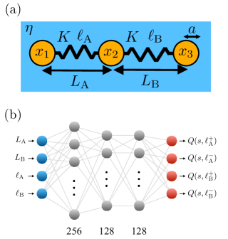
Figure 1: (a) An elastic microswimmer consists of three spheres of radius $a$ positioned along a one-dimensional coordinate system, denoted by $x_{i}$ ($i=1,2,3$). The three spheres are connected by two harmonic springs with the elastic constant $K$ and the time-dependent natural lengths $\ell_{\alpha}$ ($\alpha=\rm{A,B}$). The spring extensions are denoted by $L_{\rm A}=x_{2}-x_{1}$ and $L_{\rm B}=x_{3}-x_{2}$. The microswimmer is immersed in a viscous fluid with the shear viscosity $\eta$ and $\tau=6\pi\eta a/K$ gives the hydrodynamic relaxation time. (b) Schematic of the neural network architecture that predicts Q-values for each action from an input observation of $L_{\alpha}$ and $\ell_{\alpha}$. The blue and red columns represent the input and output layers, respectively. The grey columns are the three linear hidden layers with dimensions 256, 128, and 128.

II Elastic microswimmer with prescribed dynamics

Figure 2: The scaling function $G(\hat{\Omega})$ in Eq. (12) that describes the frequency dependence of the average swimming velocity $\overline{V}$ of an elastic swimmer with prescribed dynamics of the natural lengths given by Eqs. (9) and (10).

We first review the elastic three-sphere microswimmer model introduced by the present authors Yasuda17c ; Kuroda19 ; Era21 ; Yasuda2023 and others Pande15 ; Pande17 . As illustrated in Fig. 1(a), the microswimmer consists of three spheres of radius $a$ positioned along a one-dimensional coordinate system, denoted by $x_{i}$ ($i=1,2,3$). One can assume $x_{1}<x_{2}<x_{3}$ without loss of generality. Unlike the original three-sphere microswimmer model by Najafi and Golestanian Golestanian2004 ; Golestanian2008 , the three spheres are connected by two harmonic springs, each with a time-dependent natural length $\ell_{\alpha}$ ($\alpha=\rm{A,B}$) and having the same spring elastic constant $K$. Such an elastic microswimmer is immersed in a viscous fluid with the shear viscosity $\eta$. Although $a$ and $K$ can differ between the spheres and the springs, respectively Kobayashi23a ; Yasuda17c ; Golestanian2008 , we consider here the symmetric case. This elastic microswimmer model Yasuda17c reduces to the original three-sphere model with rigid arms Golestanian2004 ; Golestanian2008 when $K$ is infinitely large.

When the spring lengths $L_{\rm A}=x_{2}-x_{1}$ and $L_{\rm B}=x_{3}-x_{2}$ deviate from their natural lengths $\ell_{\alpha}$, the elastic forces $f_{i}$ acting on each sphere are given by

$$f_{1} =K(L_{\rm A}-\ell_{\rm A}),$$ (1)

$$f_{2} =-K(L_{\rm A}-\ell_{\rm A})+K(L_{\rm B}-\ell_{\rm B}),$$ (2)

$$f_{3} =-K(L_{\rm B}-\ell_{\rm B}).$$ (3)

Due to hydrodynamic interactions described by the Stokes mobility and the Oseen tensor, the forces $f_{i}$ and the sphere velocities $v_{i}=\dot{x}_{i}=dx/dt$ (dot indicates the time derivative) are related by Golestanian2004 ; Golestanian2008

$$v_{1} =\frac{f_{1}}{6\pi\eta a}+\frac{f_{2}}{4\pi\eta L_{\rm A}}+\frac{f_{3}}{4\pi\eta(L_{\rm A}+L_{\rm B})},$$ (4)

$$v_{2} =\frac{f_{1}}{4\pi\eta L_{\rm A}}+\frac{f_{2}}{6\pi\eta a}+\frac{f_{3}}{4\pi\eta L_{\rm B}},$$ (5)

$$v_{3} =\frac{f_{1}}{4\pi\eta(L_{\rm A}+L_{\rm B})}+\frac{f_{2}}{4\pi\eta L_{\rm B}}+\frac{f_{3}}{6\pi\eta a},$$ (6)

where the conditions $a/L_{\alpha}\ll 1$ are assumed. For the elastic microswimmer, the the force-free condition, $f_{1}+f_{2}+f_{3}=0$, is automatically satisfied, ensuring a self-propelled motion without any external force.

When $L_{\rm\alpha}$ and $\ell_{\alpha}$ are given, the dynamics of the microswimmer are deterministic and the total swimming velocity $V=(v_{1}+v_{2}+v_{3})/3$ is given by

$$V= \frac{1}{12\pi\eta}\biggl{[}\left(\frac{1}{L_{\rm A}+L_{\rm B}}-\frac{1}{L_{\rm B}}\right)f_{1}$$

$$+\left(\frac{1}{L_{\rm A}+L_{\rm B}}-\frac{1}{L_{\rm A}}\right)f_{3}\biggr{]}.$$ (7)

For relatively small deformations of the springs, we can define the small displacements with respect to the average spring length $\ell$ as $u_{\alpha}=L_{\alpha}-\ell$ ($\alpha=\rm{A,B}$). Within the small-amplitude approximation, $u_{\alpha}/\ell\ll 1$, Golestanian and Ajdari calculated the average swimming velocity of a three-sphere microswimmer up to the leading order as Golestanian2008

$$\overline{V}=\frac{7a}{24\ell^{2}}\overline{(u_{\rm A}\dot{u}_{\rm B}-\dot{u}_{\rm A}u_{\rm B})}.$$ (8)

Here the averaging, indicated by the bar, is performed by time integration in a full cycle and further divided by the total time of period. The above expression indicates that $\overline{V}$ is determined by the product of the closed loop area and the loop frequency Shapere89 .

The explicit form of $\overline{V}$ of an elastic microswimmer can be obtained by specifying a prescribed cyclic change in the natural spring lengths $\ell_{\alpha}$. Previously, we used the following sinusoidal forms Yasuda17c ; Yasuda2023

$$\ell_{\rm A} =\ell+d_{\rm A}\cos(\Omega t),$$ (9)

$$\ell_{\rm B} =\ell+d_{\rm B}\cos(\Omega t-\phi),$$ (10)

where $\ell$ is the constant natural length, $d_{\alpha}$ are the amplitudes of the oscillatory change, $\Omega$ is the common frequency, and $\phi$ is the phase difference between the two cyclic changes. When the natural lengths undergo this prescribed cycle, the spring lengths relax to their new natural lengths obeying Eqs. (1)-(6) with a hydrodynamic relaxation time $\tau=6\pi\eta a/K$.

Then the average swimming velocity of an elastic microswimmer with the prescribed dynamics was calculated to be Yasuda17c ; Yasuda2023

$$\overline{V}=\frac{7ad_{\rm A}d_{\rm B}}{24\ell^{2}\tau}G(\hat{\Omega})\sin\phi,$$ (11)

where $\hat{\Omega}=\Omega\tau$ is the dimensionless frequency and $G(\hat{\Omega})$ is the scaling function

$$G(\hat{\Omega})=\frac{3\hat{\Omega}(3+\hat{\Omega}^{2})}{9+10\hat{\Omega}^{2}+\hat{\Omega}^{4}}.$$ (12)

We see that $\overline{V}$ is non-zero when $\phi\neq 0,\pi$ corresponding to the non-reciprocal deformation, and $|\overline{V}|$ is maximized when $\phi=\pm\pi/2$.

In Fig. 2, we plot the frequency dependence of $\overline{V}$ given by Eq. (12). In the small-frequency limit of $\hat{\Omega}\ll 1$, the average velocity increases as $\overline{V}\sim\hat{\Omega}$ Golestanian2004 ; Golestanian2008 . In the larger-frequency limit of $\hat{\Omega}\gg 1$, however, the average velocity decreases as $\overline{V}\sim\hat{\Omega}^{-1}$ Yasuda17c ; Yasuda2023 . The crossover frequency between these two regimes is approximately $\hat{\Omega}\approx 1$. In the large-frequency regime, the mechanical response is delayed because it takes time for the springs to relax to their natural lengths. Such a decrease in the swimming velocity is a drawback of an elastic microswimmer as long as its internal dynamics are prescribed. A similar crossover behavior and a decrease in the average velocity were predicted for the Najafi-Golestanian microswimmer model in a viscoelastic fluid Yasuda2017 ; YasudaKuroda20 .

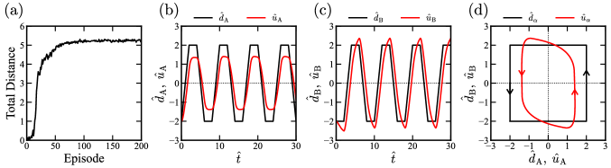
Figure 3: (a) Training curve of an elastic microswimmer when the actuation velocity is $\hat{U}=2$. The total distance achieved by the microswimmer within an episode is plotted as a function of the trained episodes. (b), (c) Periodic dynamics of the natural length deviations $\hat{d}_{\alpha}=\hat{\ell}_{\alpha}-\hat{\ell}$ (black) and the the spring extensions $\hat{u}_{\alpha}=\hat{L}_{\alpha}-\hat{\ell}$ (red) obtained from the fully trained microswimmer with 200 episodes of experience. The dimensionless time is defined by $\hat{t}=t/\tau$, and the parameters are $\hat{U}=2$ and $\hat{\ell}=10$. The oscillation phase difference between (b) and (c) is approximately $\pi/2$, with a fore-aft amplitude difference. (d) The configuration space trajectory of $\hat{d}_{\alpha}$ (black) and $\hat{u}_{\alpha}$ (red) when $\hat{U}=2$. Both $\hat{d}_{\alpha}$ and $\hat{u}_{\alpha}$ form counterclockwise cyclic loops.

III Elastic microswimmer directed by reinforcement learning

Using an elastic microswimmer model, we apply a machine learning method to direct its movement rather than prescribing the motion of the natural lengths $\ell_{\alpha}$, as described in the previous section. We combine Deep Q-Network (DQN) with reinforcement learning Dayan1992 ; mnih2013 ; sutton2018 to train the actuation of a microswimmer and obtain the optimized dynamics for the natural lengths. In particular, we shall investigate how a trained microswimmer adapts to a new strategy to avoid the decrease in the average swimming velocity when the actuation is faster than the hydrodynamic time scale $\tau$.

As shown in Fig. 1(b), our artificial intelligence (AI) uses the spring lengths $L_{\rm\alpha}$ and the natural lengths $\ell_{\rm\alpha}$ as an observation (state) input and performs an action to change either $\ell_{\rm A}$ or $\ell_{\rm B}$ with an actuation velocity $U$, i.e., the rate of changes in the natural lengths. Specifically, the output action space is discrete and consists of four actions $\ell_{\alpha}^{\pm}$ corresponding to the increase and decrease of $\ell_{\alpha}$. When the natural lengths $\ell_{\alpha}$ change, the spring lengths $L_{\alpha}$ tend to relax toward the new natural lengths according to Eqs. (1)-(6). Hereafter, we choose the sphere radius $a$ and the hydrodynamic relaxation time $\tau=6\pi\eta a/K$ as the units for length and time, respectively. The dimensionless quantities are then denoted with a hat such as $\hat{L}_{\alpha}=L_{\alpha}/a$, $\hat{\ell}_{\alpha}=\ell_{\alpha}/a$, and $\hat{U}=U\tau/a$. During the training process, we constrain the natural lengths to be in the range $8\leq\hat{\ell}_{\alpha}\leq 12$. In our model, the actuation velocity $\hat{U}$ is a control parameter and can be contrasted with the frequency $\hat{\Omega}$ in Sec. II. We train the microswimmers at different actuation velocities ranging from $\hat{U}=0.1$ to $10$, with an increment of $0.1$. Each training session comprises 200 episodes, and each episode contains 1,200 decisions made by the AI.

To optimize the locomotion of the microswimmer, we initiate each episode with a random state and employ the Epsilon Greedy Algorithm (EGA) to further balance between exploration and exploitation during training process sutton2018 . Actions are determined successively by the AI in each decision step in which the natural lengths $\hat{\ell}_{\alpha}$ are changed by $\pm 1$ with a given actuation velocity $\hat{U}$. Hence, consecutive decisions are made at intervals of $\Delta\hat{t}_{\rm dec}=1/\hat{U}$. Since the numerical time step $\Delta\hat{t}_{\rm{num}}=0.01$ is used to solve the hydrodynamic equations in Eqs. (1)-(6), the relation $\Delta\hat{t}_{\rm dec}/\Delta\hat{t}_{\rm num}=100/\hat{U}$ ensures adequate numerical time steps between successive actions for $0.1\leq\hat{U}\leq 10$.

In our model, successive actions are consistently taken at intervals of $\Delta\hat{t}_{\rm dec}$. This means that the subsequent action is executed immediately after $\hat{\ell}_{\alpha}$ has evolved by $\pm 1$, irrespective of whether the spring lengths $\hat{L}_{\alpha}$ have fully relaxed to the new natural lengths $\ell_{\alpha}$ or not. In specific situations, the machine can conduct a waiting strategy where it refrains from changing any natural lengths for $\Delta\hat{t}_{\rm{dec}}$. Such a decision arises from actions that violate the natural length constraints. For example, taking $\hat{\ell}_{\rm A}^{+}$ is not allowed when $\hat{\ell}_{\rm A}=12$, which is the maximum value in our model. In this case, no change is applied to $\hat{\ell}_{\rm A}$ and the consecutive action is conducted after $\Delta\hat{t}_{\rm dec}$.

The training process is formulated as a Markov decision process (MDP) with the memoryless property sutton2018 , ensuring that the immediate reward depends only on the current state and action. Within the MDP method, the training of the DQN is guided by Bellman’s equation that is used to iteratively update the prediction of the Q-value function (the expected cumulative future reward) in every decision step Dayan1992 ; mnih2013 ; sutton2018 . In our model, Bellman’s equation is given by

$$Q(s_{t},a_{t})=r_{t}+\gamma\max_{a^{\prime}}Q(s_{t+1},a^{\prime}),$$ (13)

where $Q(s_{t},a_{t})$ represents the Q-value of taking an action $a_{t}\in\hat{\ell}_{\alpha}^{\pm}$ in state $s_{t}=(\hat{L}_{\alpha},\hat{\ell}_{\alpha})$ at time $t$, and $r_{t}$ denotes the reward obtained after taking action $a_{t}$ in state $s_{t}$. The reward is defined as the positive displacement of the whole microswimmer during a decision step. The coefficient $\gamma$ represents the discount factor that balances the importance between immediate rewards and future rewards. We choose $\gamma=0.99$ for farsightedness to prioritize long-term cumulative rewards. By updating the network with Bellman’s equation in every decision step, our DQN efficiently learns the optimal policy for controlling the dynamics of the natural lengths $\hat{\ell}_{\alpha}$.

In Fig. 3(a), we show the training curve of a microswimmer when the actuation velocity is $\hat{U}=2$. As a function of the trained episodes, we plot the total distance, namely, the net displacement from the initial position that the microswimmer can achieve within an episode. During the training process, the total distance continuously increases over the episodes, indicating enhanced locomotion ability. After about 100 episodes, the microswimmer reaches an optimal swimming distance within the fixed total time. The small fluctuations that remain after reaching the optimal total distance are due to random initial conditions and EGA used for the training. Details of the training process will be separately discussed later in Sec. V.

IV Fully trained elastic microswimmer

In this section, we discuss the dynamic properties of the microswimmers which have been trained for 200 episodes. Besides the emergence of limit cycles, we shall discuss the performance and effective odd elasticity of trained microswimmers.

IV.1 Emergence of limit cycles

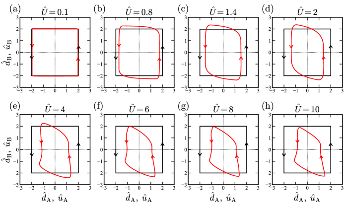
Figure 4: Limit cycles of microswimmers trained with different $\hat{U}$-values ranging from $0.1$ to $10$. Black and red lines represent the natural length deviations $\hat{d}_{\alpha}$ and the spring extensions $\hat{u}_{\alpha}$, respectively. The plot in (d) for $\hat{U}=2$ is identical to that in Fig. 3(d).

Figure 5: The dimensionless spring amplitudes $|\hat{u}_{\alpha}|$ as a function of $\hat{U}$. These amplitudes exhibit fore-aft asymmetry.

Figure 6: Performance of the fully trained microswimmer at various actuation velocities $\hat{U}$. (a) The dimensionless non-reciprocality $\hat{R}=R/a^{2}$ defined in Eq. (14) as a function of $\hat{U}$. This quantity represents the enclosed area of the red loops made of $u_{\alpha}$ in Fig. 4. (b) The dimensionless loop frequency $1/\hat{T}=\tau/T$ as a function of $\hat{U}$. When $\hat{U}\leq 2$, the loop frequency increases linearly with $\hat{U}$ as fitted by the dotted line ($1/\hat{T}=\hat{U}/16$). (c) The dimensionless cycle performance $\hat{R}/\hat{T}$ (calculated from (a) and (b)) as a function of $\hat{U}$. (d) The dimensionless average swimming velocity $\hat{\overline{V}}=\overline{V}\tau/a$ as a functions of $\hat{U}$. Both $\hat{R}/\hat{T}$ in (c) and $\hat{\overline{V}}$ in (d) show the same $\hat{U}$-dependence except a numerical factor. The ratio between these quantities is $\hat{\overline{V}}\hat{T}/\hat{R}\approx 6.57\times 10^{-3}$. The interpretation of this ratio is discussed in the text.

In Figs. 3(b) and (c), we present the cyclic motions of the fully trained swimmer when $\hat{U}=2$. The black lines represent the deviation of the natural lengths from its average value, i.e., $\hat{d}_{\alpha}=\hat{\ell}_{\alpha}-\hat{\ell}$ ($\alpha=\rm{A,B}$), where we chose $\hat{\ell}=10$ because we have the constraint $8\leq\hat{\ell}_{\alpha}\leq 12$. The red lines represent the spring extensions $\hat{u}_{\alpha}=\hat{L}_{\alpha}-\hat{\ell}$ ($\alpha=\rm{A,B}$). Both $\hat{u}_{\rm A}$ and $\hat{u}_{\rm B}$ in Figs. 3(b) and (c), respectively, exhibit periodic motions with a phase difference of approximately $\pi/2$, corresponding to the maximum efficiency for swimming.

In Fig. 3(d), we present the configuration space trajectory of the same trained microswimmer over one cycle. The trajectory of the natural lengths $\hat{d}_{\alpha}$ (shown in black) forms a counterclockwise square in the range $-2\leq\hat{d}_{\alpha}\leq 2$. The spring extensions $\hat{u}_{\alpha}$ (shown in red) also exhibit a limit cycle in the configuration space. This means that the fully trained elastic microswimmer has acquired non-reciprocal spring motion owing to training, and performs effective locomotion through the optimized limit cycle.

To investigate the dependence on the actuation velocity $\hat{U}$, we plot in Figs. 4(a)-(h) the configuration space trajectories for different values ranging from $\hat{U}=0.1$ to $10$ (Fig. 4(d) and Fig. 3(d) are the same). In all the cases, the natural lengths $\hat{d}_{\alpha}$ (shown in black) follow the same counterclockwise square shape. When the actuation velocity is small, such as $\hat{U}\leq 2$ in Figs. 4(a)-(d), the hydrodynamic relaxation process can catch up with the change in the natural lengths, and the cycles of the spring extensions $\hat{u}_{\alpha}$ (shown in red) are close to the square-shaped trajectory. In this regime, the enclosed area within the loop decreases when $\hat{U}$ is increased, as we quantify in the next subsection.

For larger actuation velocity $\hat{U}>2$, corresponding to Figs. 4(e)-(h), the hydrodynamic relaxation becomes the slower mode. This situation is similar to the case of $\hat{\Omega}>1$ in Sec. II. For the trained microswimmer, however, the AI adapts a waiting strategy once the natural lengths reach the maximum or minimum values ($\hat{d}_{\alpha}=\pm 2$) in order for the spring extensions $\hat{u}_{\alpha}$ to relax sufficiently.

This waiting strategy allows the spring lengths to catch up with the large actuation velocity $\hat{U}$ and to prevent the enclosed area from further decreasing.

Since the dynamics are no longer dominated by the actuation velocity $\hat{U}$, the trajectories of $\hat{u}_{\alpha}$ become less squared and less symmetric for $\hat{U}>2$. As a result, the distinctions between different loop shapes become less pronounced in Figs. 4(e)-(h).

Another notable result in Fig. 4 is the fore-aft amplitude asymmetry between $\hat{u}_{\rm A}$ and $\hat{u}_{\rm B}$. In Fig. 5, we plot the amplitudes $|\hat{u}_{\alpha}|$ as a function of $\hat{U}$. Starting from the value $|\hat{u}_{\alpha}|=2$, $|\hat{u}_{\rm A}|$ and $|\hat{u}_{\rm B}|$ decreases and increases, respectively, as $\hat{U}$ is increased. Notice that the maximum amplitude can be up to $|\hat{u}_{\rm B}|/\hat{\ell}\approx 0.25$. When $\hat{U}>2$, however, $|\hat{u}_{\alpha}|$ are almost independent of $\hat{U}$. The asymmetric fore-aft amplitude arises from the non-reciprocal swimming cycle, which is linked to the asymmetric order in which $\ell_{\alpha}$ changes.

IV.2 Cycle performance and swimming velocity

Next, we discuss the performance of the acquired cyclic motion and the average swimming velocity of the fully trained microswimmers. Following our work on catalytic enzymes Yasuda21-a ; Kobayashi23b , we consider the following quantity called non-reciprocality

$$R=\frac{1}{2}\int_{0}^{T}dt\,(u_{\rm A}\dot{u}_{\rm B}-\dot{u}_{\rm A}u_{\rm B}),$$ (14)

where $T$ is the period of one cycle. We note again that $R$ represents the area enclosed by the loop trajectory in the configuration space Shapere89 . Then the dimensionless average velocity $\hat{\overline{V}}=\overline{V}\tau/a$ obtained from Eq. (8) can be rewritten in terms of the dimensionless non-reciprocality $\hat{R}=R/a^{2}$ as

$$\hat{\overline{V}}=\frac{7}{12\hat{\ell}^{2}}\frac{\hat{R}}{\hat{T}},$$ (15)

where $\hat{T}=T/\tau$. We shall call $1/\hat{T}$ as the dimensionless loop frequency. The quantity $\hat{R}/\hat{T}$ can be regarded as the performance of a cyclic motion and directly determines the swimming velocity when the deformation is small.

In Fig. 6(a), we plot the non-reciprocality $\hat{R}$ as a function of $\hat{U}$ for fully trained microswimmers. As indicated in Fig. 4, the enclosed area $\hat{R}$ decreases as $\hat{U}$ increases. In Fig. 6(b), the loop frequency $1/\hat{T}$ is plotted as a function of $\hat{U}$. When $\hat{U}\leq 2$, the loop frequency increases linearly with $\hat{U}$ (shown by the dotted line) to minimize the loop period. For $\hat{U}>2$, however, the dependence of $1/\hat{T}$ on $\hat{U}$ deviates from the linear relation. This is because the actuation velocity $\hat{U}$ outpaces the hydrodynamic relaxation rate, and the AI adapts the waiting strategy to adjust to the slow hydrodynamic mode. The slope of the dashed line is $1/16$ ($1/\hat{T}=\hat{U}/16$), and hence the dimensionless waiting time at $\hat{d}_{\alpha}=\pm 2$ is estimated by $\hat{T}-16/\hat{U}$. The finite waiting time appears as a transition for $U>2$. The actual performance of the microswimmer can be evaluated by the quantity $\hat{R}/\hat{T}$, as plotted in Fig. 6(c) as a function of $\hat{U}$. We find that the cycle performance increases monotonically with $\hat{U}$ and eventually approaches the value $\hat{R}/\hat{T}\approx 1.75$ that is bounded by the hydrodynamic relaxation process.

To check the validity of Eq. (15), we plot in Fig. 6(d) the average swimming velocity $\hat{\overline{V}}$ obtained from the actual displacement of the microswimmers. Clearly, both $\hat{R}/\hat{T}$ and $\hat{\overline{V}}$ in Figs. 6(c) and (d), respectively, show almost the same dependence on $\hat{U}$ except the numerical factor. The obtained ratio from Figs. 6(c) and (d) is $\hat{\overline{V}}\hat{T}/\hat{R}\approx 6.57\times 10^{-3}$ within the studied $\hat{U}$-range. This value can be compared with the geometrical pre-factor $7/(12\hat{\ell}^{2})\approx 5.83\times 10^{-3}$ in Eq. (15) when $\hat{\ell}=10$. A small difference between these pre-factors comes from the assumption $u_{\alpha}/\ell\ll 1$ used in Eq. (8) or Eq. (15). As already shown in Fig. 5, the spring deformations can be $\hat{u}_{\alpha}/\hat{\ell}\approx 0.2$ or even larger for our trained microswimmers. Hence higher order contributions need to be taken into account in Eq. (15) to reproduce the average swimming velocity achieved by reinforcement learning.

The behavior of $\overline{V}$ in Fig. 6(d) for the trained microswimmer is in sharp contrast to that of an elastic microswimmer whose natural spring motions are prescribed. In Sec. II, we showed in Eq. (11) and Fig. 2 that the average velocity decreases when $\hat{\Omega}>1$ Yasuda17c ; Yasuda2023 . For the fully trained microswimmer, however, the AI adapts a waiting strategy for $\hat{U}>2$ and the swimming velocity does not decrease even for larger actuation velocity $\hat{U}$. Such an efficient strategy is possible when the microswimmer is directed by the machine learning scheme.

IV.3 Effective even and odd elasticities

Figure 7: (a) The effective off-diagonal even elasticity $\hat{k^{\prime}}=k^{\prime}/K$ for fully trained microswimmers as a function of $\hat{U}$ [see Eq. (19)]. The $\hat{U}$-dependence is similar to that of the non-reciprocality $\hat{R}$ in Fig. 6(a). (b) The effective odd elasticity $\hat{k}^{\rm o}=k^{\rm o}/K$ as a function of $\hat{U}$ [see Eq. (20)]. The $\hat{U}$-dependence closely resembles that of the loop frequency $1/\hat{T}$ in Fig. 6(b).

Finally, we explain the method to extract the effective even and odd elasticities of the trained microswimmer from the numerical data. A direct way is to assume the following odd-elastic Hookean relations between the forces and the spring extensions Yasuda22 ; Kobayashi23b ; Fruchart2021 :

$$\begin{pmatrix}F_{\rm A}\\ F_{\rm B}\end{pmatrix}=\begin{pmatrix}k^{\rm e}&k^{\prime}+k^{\rm o}\\ k^{\prime}-k^{\rm o}&k^{\rm e}\end{pmatrix}\begin{pmatrix}u_{\rm A}\\ u_{\rm B}\end{pmatrix}.$$ (16)

In the above, the forces $F_{\alpha}$ are given by the Stokes’ law $F_{\alpha}=-6\pi\eta a\dot{u}_{\alpha}$ and $u_{\alpha}=L_{\alpha}-\ell$ as before. In the elastic matrix, $k^{\rm e}$ and $k^{\prime}$ represent the diagonal and off-diagonal even elasticities, respectively, while $k^{\rm o}$ represents the effective odd elasticity. The diagonal even elasticity $k^{\rm e}$ should be distinguished from the spring elastic constant $K$ in the elastic microswimmer model. Given the fact that our data demonstrate sustained oscillations without amplitude decay, we assume in the following that $k^{\rm e}$ vanishes, i.e., $k^{\rm e}=0$. The off-diagonal even elasticity $k^{\prime}$ quantifies the fore-aft amplitude asymmetry as described in Fig. 5, whereas the odd elasticity $k^{\rm o}$ quantifies the non-reciprocal dynamics of the microswimmer Kobayashi23b ; Yasuda22 .

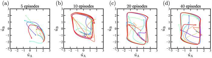
Figure 8: The configuration space trajectories at different training stages; (a) 5, (b)10, (c) 20, and (d) 40 episodes for a microswimmer with $\hat{U}=2$. Each trajectory is initiated from a distinct initial state, indicated by different colored dots. Training beyond the stage (d) aims to approach the optimized limit cycle shown in Fig. 4(d) for 200 episodes.

To obtain $k^{\prime}$ and $k^{\rm o}$ from the numerical data, we calculate the cross-correlations $\overline{F_{\rm A}u_{\rm B}}$ and $\overline{F_{\rm B}u_{\rm A}}$ averaged over one period of the deformation cycle. This is possible since the trained dynamics for the two springs are periodic with the same frequency and a finite phase difference. Since these correlations are given by

$$\overline{F_{\rm A}u_{\rm B}} =\left(k^{\prime}+k^{\rm o}\right)\overline{u^{2}_{\rm B}},$$ (17)

$$\overline{F_{\rm B}u_{\rm A}} =\left(k^{\prime}-k^{\rm o}\right)\overline{u^{2}_{\rm A}},$$ (18)

the effective (off-diagonal) even and odd elastic coefficients can be obtained from

$$k^{\prime} =\frac{1}{2}\left(\frac{\overline{F_{\rm A}u_{\rm B}}}{\overline{u_{\rm B}^{2}}}+\frac{\overline{F_{\rm B}u_{\rm A}}}{\overline{u_{\rm A}^{2}}}\right),$$ (19)

$$k^{\rm o} =\frac{1}{2}\left(\frac{\overline{F_{\rm A}u_{\rm B}}}{\overline{u_{\rm B}^{2}}}-\frac{\overline{F_{\rm B}u_{\rm A}}}{\overline{u_{\rm A}^{2}}}\right),$$ (20)

where all the related correlations can be directly calculated from the numerical data.

In Figs. 7(a) and (b), we plot dimensionless even elasticity $\hat{k}^{\prime}=k^{\prime}/K$ and odd elasticity $\hat{k}^{\rm o}=k^{\rm o}/K$, respectively, as a function of $\hat{U}$. Both $\hat{k}^{\prime}$ and $\hat{k}^{\rm o}$ vanish when $\hat{U}=0$. We recognize that the behavior of $\hat{k}^{\prime}$ is similar to that of $\hat{R}$ in Fig. 6(a) (except a constant shift), while the data of $\hat{k}^{\rm o}$ closely resembles that of $1/\hat{T}$ in Fig. 6(b). These results indicate that $\hat{k}^{\prime}$ characterizes the extent of amplitude asymmetry that decreases the enclosed area, while $\hat{k}^{\rm o}$ directly reflects the loop frequency. Since $1/\hat{T}\propto\hat{k}^{\rm o}$, we confirm that the average swimming velocity $\overline{V}$ in Eq. (15) is proportional to the odd elasticity $k^{\rm o}$, i.e., $\overline{V}\propto k^{\rm o}$. Notably, the odd elasticity $\hat{k}^{\rm o}$ is proportional to the actuation velocity up to $\hat{U}\leq 2$, similar to $1/\hat{T}$. These results clearly demonstrate the emergence of odd elasticity in microswimmers directed by deep reinforcement learning.

The fact that the effective odd elasticity $\hat{k}^{\rm o}$ is proportional to the loop frequency $1/\hat{T}$ is consistent with our model of a stochastic odd microswimmer in which the presence of odd elasticity was implemented Yasuda21 ; Kobayashi23a . In the odd microswimmer model, the probability flux forms a closed loop and the eigenvalues of the corresponding frequency matrix are proportional to the odd elasticity. For the time-correlation functions in general odd Langevin systems Yasuda22 , it was shown that odd elasticity determines the frequency of the sinusoidal component both in their symmetric and anti-symmetric parts. All these results are in accordance with the original claim that the work per cycle is generally given by the product of odd elasticity and closed loop area in active systems Scheibner2020OddElasticity ; Fruchar2023 .

V Training progression of elastic microswimmer

In this section, we discuss briefly the dynamic evolution of swimming behavior during the training process. The plots in Figs. 8(a)-(d) illustrate the configuration space trajectories $\hat{u}_{\alpha}$ ($\alpha=\rm{A,B}$) at distinct stages of training in Fig. 3(a), namely, 5, 10, 20, and 40 episodes, respectively, when $\hat{U}=2$. Each trajectory starts from a different initial state denoted by colored dots.

In the initial stage of training, as shown in Fig. 8(a), the swimming behavior is relatively restricted. Starting from different initial states, the system only evolves towards the point $(2,-2)$, showing limited exploration of the motion possibilities. This early stage primarily focuses on optimizing short-term rewards and cyclic motion does not emerge yet. As the microswimmer gains more training experience, its behavior progressively improves. After approximately 10 episodes, as shown in Fig. 8(b), the microswimmer begins to explore long-term rewards accessible through cyclic motions. Enclosed loops emerge in the configuration space, and the microswimmer starts to recognize the dynamics required for sustainable cyclic locomotion.

In Fig. 8(c) at around 20 training episodes, the shape of loops becomes clearer and more refined. This stage shows the swimmer’s ability to fine-tune its motion strategy toward the optimal cyclic pattern to maximize long-term rewards. After training for 40 episodes, the microswimmer achieves the optimized limit cycle as shown in Fig. 8(d). Importantly, this optimized cycle is robust across various initial conditions, and it will eventually approach the limit cycle shown in Fig. 4(d). Notice that the effective odd elasticity discussed in the previous section can be extracted for fully trained microswimmers after such as 200 episodes.

VI Summary and discussion

Using deep reinforcement learning (Deep Q-Network), we have investigated how effective odd elasticity emerges when optimizing the swimming ability of a model elastic microswimmer Pande15 ; Pande17 ; Yasuda17c . One of the key findings is the optimized natural-length dynamics without the need for prescribed motion. Notably, we observed a strategy transition when the actuation velocity is $\hat{U}\approx 2$ (Fig. 4). For larger $\hat{U}$, the trained microswimmers adapt to the hydrodynamic slow relaxation and avoid the velocity decrease. This waiting strategy significantly improves the swimming ability compared to the elastic microswimmer with prescribed dynamics having large-frequency oscillations. The trained microswimmer exhibits fore-aft asymmetry in the spring amplitudes (Fig. 5), which is generally difficult to predict and implement in the prescribed dynamics.

By calculating the force-displacement correlations for fully trained microswimmers, we have extracted the effective even and odd elasticities, $k^{\prime}$ and $k^{\rm o}$, respectively (Fig. 7). We have shown that the $U$-dependencies of $k^{\prime}$ and $k^{\rm o}$ closely resemble to those of the non-reciprocality $R$ in Fig. 6(a) and the loop frequency $1/T$ in Fig. 6(b), respectively. From the numerical data, we have further confirmed that the average swimming velocity $\overline{V}$ is proportional to the cycle performance $R/T$, (Figs. 6(c) and (d)), as predicted in Eq. (15). These results clarify the proportionality relation between the average velocity and odd elasticity, $\overline{V}\propto k^{\rm o}$. Our study offers a way to reveal the emergence of odd elasticity in various active systems using a machine learning approach.

If we assume that the energy injected through the non-reciprocal process balances with the dissipation due to the net motion of a microswimmer, its power (work per unit time) scales as $\dot{W}\sim(\eta a\overline{V})\times\overline{V}\propto(k^{\rm o})^{2}$. Here, $\eta a\overline{V}$ corresponds to the dissipative force, and we have used the relation $\overline{V}\propto k^{\rm o}$ Kobayashi23b . For an odd microswimmer, it was further shown that all the extracted work due to odd elasticity is converted into the entropy production rate Yasuda21 . Hence, odd elasticity is useful to characterize non-reciprocal dynamics of active micromachines, including not only microswimmers but also other molecular motors Yasuda22-machlup ; Yasuda22 .

In our machine learning model, we adopted a relatively simple discrete Deep Q-Network (DQN) algorithm to train elastic microswimmers. Since the swimming ability is directly related to the strength of non-reciprocal forces, the optimized dynamics are to adjust one of the natural lengths to either its maximum or minimum value before changing the other. For such strategies, the microswimmer does not need to change the two natural lengths simultaneously and continuous-action algorithms are unnecessary. To validate this argument, we have also employed the other continuous-action algorithms such as Deep Deterministic Policy Gradient (DDPG) Lillicrap2015 and Soft Actor-Critic (SAC) Haarnoja2018 . Both of these methods resulted in the same strategy as the discrete DQN algorithm. Although these continuous-action algorithms are helpful for more complicated microswimmers, the discrete DQN algorithm used in this work is sufficient for an elastic microswimmer moving in a one-dimensional space.

Microswimmers composed of biomaterials are often soft and exhibit viscoelastic responses. This softness is crucial not only because of the inevitable interaction with viscoelastic environments but also due to their versatile functionalities schamel2014 ; walker2015 ; wu2018 ; medina2018 ; huang2019 ; Striggow2020 ; soto2022 , such as mechanical signal sensing xu2019 ; huo2020 , cargo loading and unloading alapan2028 ; xu2020 , and navigation through intricate channels vutukuri2020 . Hence, a crossover between the elasticity and viscosity generally exists for the large- and small-frequency limits of microswimmers. For such systems, we have shown that a transition in the swimming strategy around the crossover actuation velocity is desired for the optimized performance because a simple prescribed periodic motion becomes less efficient in the large-frequency regime. The strategy transition found in this paper can generally exist in various other microswimmer models.

Finally, we comment that the even and odd elasticities obtained from the numerical data are assumed to be linear. In a more general scenario, however, these elasticities can be non-linear Fruchar2023 . Since a diagonal positive elasticity generally leads to a decaying oscillation Lin23 , non-linearity is commonly required for odd-elastic systems to exhibit a stable limit cycle Ishimoto22 . The inclusion of non-linear elasticity can describe more general cases such as the spontaneous onset of oscillations with a specific amplitude that is regulated by the ratio of linear and non-linear even elasticities Ishimoto23 . In the present work, the oscillation amplitudes are determined by the constraint that clips the natural lengths, and hence the linear approach is more suitable.

Applications that use machine learning to optimize gait-switching for microswimmer navigation have been widely studied in the recent literatures cichos2020 ; stark2021 ; hartl2021 ; stark2023 ; alageshan2020 ; landin2021 ; schneider2019 ; nasiri2023 ; tsang2020 ; zou2022 ; qin2023 ; liu2023 ; borra2022 ; zhu2022 . These works have provided strong insight into the value that machine learning can discover for the optimized dynamics of microswimmers. Besides focusing on performance optimization, we have emphasized the possibility of extracting useful information such as non-reciprocality and odd elasticity. In future studies, we aim to establish universal relations between performance and odd elasticity for different types of microswimmers Laugabook .

- (1) M. C. Marchetti, J. F. Joanny, S. Ramaswamy, T. B. Liverpool, J. Prost, M. Rao, and R. A. Simha, Rev. Mod. Phys. 85, 1143 (2013).
- (2) G. Gompper et al., J. Condens. Matter Phys. 32, 193001 (2020).
- (3) S. Shankar, A. Souslov, M. J. Bowick, M. C. Marchetti, and V. Vitelli, Nat. Rev. Phys. 4, 380-398 (2022).
- (4) K. K. Dey, Angew. Chem. Int. Ed. 58, 2208 (2019).
- (5) Y. Hosaka and S. Komura, Biophys. Rev. Lett. 17, 51 (2022).
- (6) K. K. Dey, F. Wong, A. Altemose, and A. Sen, Curr. Opin. Colloid Interface Sci. 21, 4 (2016).
- (7) H. Y. Aviram, M. Pirchi, H. Mazal, Y. Barak, I. Riven and G. Haran, Proc. Natl. Acad. Sci. U. S. A. 115, 3243 (2018).
- (8) C. Echeverria, Y. Togashi, A. S. Mikhailov, and R. Kapral, Phys. Chem. Chem. Phys. 13, 10527 (2011).
- (9) A. S. Mikhailov and R. Kapral, Proc. Natl. Acad. Sci. U. S. A. 112, E3639 (2015).
- (10) Y. Hosaka, S. Komura, and A. S. Mikhailov, Soft Matter 16, 10734-10749 (2020).
- (11) K. Yasuda and S. Komura, Phys. Rev. E 103, 062113 (2021).
- (12) A. Kobayashi, K. Yasuda, K. Ishimoto, L.-S. Lin, I. Sou, Y. Hosaka, and S. Komura, J. Phys. Soc. Jpn. 92, 074801 (2023).
- (13) E. M. Purcell, Am. J. Phys. 45, 3 (1977).
- (14) E. Lauga and T. R. Powers, Rep. Prog. Phys. 72, 096601 (2009).
- (15) E. Lauga, The Fluid Dynamics of Cell Motility, (Cambridge Univ. Press, Cambridge, 2020)
- (16) M. Leoni and P. Sens, Phys. Rev. E 91, 022720 (2015).
- (17) M. Leoni and P. Sens, Phys. Rev. Lett. 118, 228101 (2017).
- (18) M. Tarama and R. Yamamoto, J. Phys. Soc. Jpn. 87, 044803 (2018).
- (19) C. Scheibner, A. Souslov, D. Banerjee, P. Surówka, W. T. Irvine, and V. Vitelli, Nat. Phys. 16, 475 (2020).
- (20) M. Fruchart, C. Scheibner, and V. Vitelli, Annu. Rev. Condens. Matter Phys.14, 471-510 (2023).
- (21) L. Braverman, C. Scheibner, B. VanSaders, and V. Vitelli, Phys. Rev. Lett. 127, 268001 (2021).
- (22) E. S. Bililign, F. B. Usabiaga, Y. A. Ganan, A. Poncet, V. Soni, S. Magkiriadou, M. J. Shelley, D. Bartolo, and W. T. Irvine, Nat. Phys. 8, 212-218 (2022).
- (23) P Surówka, A Souslov, F Jülicher, and D Banerjee, arXiv:2210.13606
- (24) M. Fossati, C. Scheibner, M. Fruchart, and V. Vitelli, arXiv:2210.03669
- (25) T. H. Tan, A. Mietke, J. Li, Y. Chen, H. Higinbotham, P. J. Foster, S. Gokhale, J. Dunkel, and N. Fakhri, Nature 607, 287 (2022).
- (26) K. Ishimoto, C. Moreau, and K. Yasuda, Phys. Rev. E 105, 064603 (2022).
- (27) K. Ishimoto, C. Moreau, and K. Yasuda, PRX Life 1, 023002 (2023).
- (28) M. Brandenbourger, C. Scheibner, J. Veenstra, V. Vitelli, and C. Coulais, arXiv:2108.08837
- (29) K. Yasuda, A. Kobayashi, L.-S. Lin, Y. Hosaka, I. Sou, and S. Komura, J. Phys. Soc. Jpn. 91, 015001 (2022).
- (30) K. Yasuda, K. Ishimoto, A. Kobayashi, L.-S. Lin, I. Sou, Y. Hosaka, and S. Komura, J. Chem. Phys. 157, 095101 (2022).
- (31) K. Yasuda, Y. Hosaka, I. Sou, and S. Komura, J. Phys. Soc. Jpn. 90, 075001 (2021).
- (32) N. Mitarai, H. Hayakawa, and H. Nakanishi, Phys. Rev. Lett. 88, 174301 (2002).
- (33) M. Doi, Soft Matter Physics (Oxford University Press, Oxford 2013).
- (34) L.-S. Lin, K. Yasuda, K. Ishimoto, Y. Hosaka, and S. Komura, J. Phys. Soc. Jpn. 92, 033001 (2023).
- (35) M. Fruchart, R. Hanai, P. B. Littlewood, and V. Vitelli, Nature 592, 363 (2021).
- (36) K. Yasuda, Y. Hosaka, M. Kuroda, R. Okamoto, and S. Komura, J. Phys. Soc. Jpn. 86, 093801 (2017).
- (37) J. Pande and A.-S. Smith, Soft Matter 11, 2364 (2015).
- (38) J. Pande, L. Merchant, T. Krüger, J. Harting, and A.-S. Smith, New J. Phys. 19, 053024 (2017).
- (39) F. Cichos, K. Gustavsson, B. Mehlig, and G. Volpe, Nat. Mach. Intell. 2, 94 (2020).
- (40) H. Stark, Sci Robot. 6, eabh1977 (2021).
- (41) B. Hartl, M. Hübl, G. Kahl, and A. Zöttl, Proc. Natl Acad. Sci. USA 118, e2019683118 (2021).
- (42) M. Putzke and H. Stark, Eur. Phys. J. E 46, 48 (2023).
- (43) E. Schneider and H. Stark, EPL 127, 64003 (2019).
- (44) J. K. Alageshan, A. K. Verma, J. Bec, and R. Pandit, Phys. Rev. E 101, 043110 (2020).
- (45) S. Muiños-Landin, A. Fischer, V. Holubec, and F. Cichos, Sci. Robot. 6, eabd9285 (2021).
- (46) M. Nasiri, H. Löwen, and B. Liebchen, EPL 142, 17001 (2023).
- (47) A. C. H. Tsang, P. W. Tong, S. Nallan, and O. S. Pak, Phys. Rev. Fluids 5, 074101 (2020).
- (48) Z. Zou, Y. Liu, Y.-N. Young, O. S. Pak, and A. C. H. Tsang, Commun. Phys. 5, 158 (2022).
- (49) K. Qin, Z. Zou, L. Zhu, and O. S. Pak, Phys. Fluids 35, 032003 (2023).
- (50) F. Borra, L. Biferale, M. Cencini, and A. Celani, Phys. Rev. Fluids 7, 023103 (2022).
- (51) G. Zhu, W. Z. Fang, and L. Zhu, J. Fluid Mech. 944, A3 (2022).
- (52) Y. Liu, Z. Zou, O. S. Pak, and A. C. H. Tsang, Sci. Rep. 13, 9397 (2023).
- (53) M. Kuroda, K. Yasuda, and S. Komura, J. Phys. Soc. Jpn. 88, 054804 (2019).
- (54) K. Era, Y. Koyano, Y. Hosaka, K. Yasuda, H. Kitahata, and S. Komura, EPL 133, 34001 (2021).
- (55) K. Yasuda, Y. Hosaka, and S. Komura, J. Phys. Soc. Jpn. 92, 121008 (2023).
- (56) A. Najafi and R. Golestanian, Phys. Rev. E 69, 062901 (2004).
- (57) R. Golestanian and A. Ajdari, Phys. Rev. E 77, 036308 (2008).
- (58) A. Kobayashi, K. Yasuda, L.-S. Lin, I. Sou, Y. Hosaka, and S. Komura, J. Phys. Soc. Jpn. 92, 034803 (2023).
- (59) A. Shapere and F. Wilczek, J. Fluid Mech. 198, 557 (1989).
- (60) K. Yasuda, R. Okamoto, and S. Komura, J. Phys. Soc. Jpn. 86, 043801 (2017).
- (61) K. Yasuda, M. Kuroda, and S. Komura, Phys. Fluids 32, 093102 (2020).
- (62) C. J. Watkins and P. Dayan, Mach. Learn. 8, 279-292 (1992).
- (63) V. Mnih, K. Kavukcuoglu, D. Silver, A. Graves, I. Antonoglou, D. Wierstra, and M. Riedmiller, arXiv:1312.5602
- (64) R. S. Sutton and A. G. Barto, Reinforcement Learning: An Introduction (MIT Press, Cambridge, 2018).
- (65) T. P. Lillicrap, J. J. Hunt, A. Pritzel, N. Heess, T. Erez, Y. Tassa, D. Silver, and D Wierstra, arXiv:1509.02971
- (66) T. Haarnoja, A. Zhou, P. Abbeel, and S. Levine, PMLR 80, 1861-1870 (2018).
- (67) D. Schamel , A. G. Mark, J. G. Gibbs, C. Miksch, K. I. Morozov, A. M. Leshansky, and P. Fischer, ACS Nano 8, 8794-8801 (2014).
- (68) D. Walker, B. T. Käsdorf, H. H. Jeong, O. Lieleg, and P. Fischer, Sci. Adv. 1, e1500501 (2015).
- (69) Z. Wu, J. Troll, H.-H. Jeong, Q. Wei, M. Stang, F. Ziemssen, Z. Wang, M. Dong, S. Schnichels, T. Qiu, and P. Fischer, Sci. Adv. 4, eaat4388 (2018).
- (70) M. Medina-Sánchez, V. Magdanz, M. Guix, V. M. Fomin, and O. G. Schmidt, Adv. Funct. Mater. 28, 1707228 (2018).
- (71) H. W. Huang, F. E. Uslu, P. Katsamba, E. Lauga, M. S. Sakar, and B. J. Nelson, Sci. Adv. 5, eaau1532 (2019).
- (72) F. Striggow, M. Medina-Sánchez, G. K. Auernhammer, V. Magdanz, B. M. Friedrich, and O. G. Schmidt, Small 16, 2000213 (2020).
- (73) F. Soto, E. Karshalev, F. Zhang, B. E. F. de Avila, A. Nourhani, and J. Wang, Chem. Rev. 122, 5, 5365-5403 (2022).
- (74) T. Xu, J. Zhang, M. Salehizadeh, O. Onaizah, and E. Diller, Sci. Robot. 4, eaav4494 (2019).
- (75) X. Huo, Y. Wu, A. Boymelgreen, and G. Yossifon, Langmuir 36, 6963-6970 (2020).
- (76) Y. Alapan, O. Yasa, O. Schauer, J. Giltinan, A. F. Tabak, V. Sourjik, and M. Sitti, Sci. Robot. 3, eaar4423 (2018).
- (77) H. Xu, M. Medina-Sánchez, M. F. Maitz, C. Werner, and O. G. Schmidt, ACS Nano 14, 2982-2993 (2020).
- (78) H. R. Vutukuri, M. Hoore, C. Abaurrea-Velasco, L. van Buren, A. Dutto, T. Auth, D. A. Fedosov, G. Gompper, and J. Vermant, Nature 586, 52-56 (2020).