The continuum limit of k-space cavity angular momentum is controlled by an infinite range difference operator.

Abstract

A wavepacket (electromagnetic or otherwise) within an isotropic and homogeneous space can be quantized on a regular lattice of discrete $\mathbf{k}$-vectors. Each $\mathbf{k}$-vector is associated with a temporal frequency $\omega$; together, $\mathbf{k}$ and $\omega$ represent a propagating plane-wave. While the total energy and total linear momentum of the packet can be readily apportioned among its individual plane-wave constituents, the same cannot be said about the packet’s total angular momentum. One can show, in the case of a reasonably smooth (i.e., continuous and differentiable) wave packet, that the overall angular momentum is expressible as an integral over the k-space continuum involving only the Fourier transform of the field and its $\mathbf{k}$-space gradients. In this sense, the angular momentum is a property not of individual plane-waves, but of plane-wave pairs that are adjacent neighbors in the space inhabited by the $\mathbf{k}$-vectors, and can be said to be localized in the $\mathbf{k}$-space. Strange as it might seem, this hallmark property of angular momentum does not automatically emerge from an analysis of a discretized $\mathbf{k}$-space. In fact, the discrete analysis shows the angular momentum to be distributed among $\mathbf{k}$-vectors that pair not only with nearby $\mathbf{k}$-vectors but also with those that are far away. The goal of the present paper is to resolve the discrepancy between the discrete calculations and those performed on the continuum, by establishing the conditions under which the highly non-local sum over plane-wave pairs in the discrete $\mathbf{k}$-space would approach the localized distribution of the angular momentum across the continuum of the $\mathbf{k}$-space.

1 Introduction

According to the classical theory of electrodynamics, an electromagnetic (EM) wavepacket propagating in free space carries energy, linear momentum, and angular momentum ^{4, 5, 10, 11, 12, 13, 16}. The knowledge of the wavepacket’s electric-field profile in spacetime, $\mathbf{E}(\mathbf{r},t)$, is generally all that is needed to compute its remaining physical properties⁷. The magnetic field distribution $\mathbf{H}(\mathbf{r},t)$ is readily computable from the (four-dimensional) Fourier transform of $\mathbf{E}(\mathbf{r},t)$, whence the Poynting vector $\mathbf{S}(\mathbf{r},t)=\mathbf{E}(\mathbf{r},t)\crossproduct\mathbf{H}(\mathbf{r},t)$ yields the rate of flow of EM energy per unit area per unit time⁷. The linear momentum density is subsequently determined as $\mathbf{P}(\mathbf{r},t)=\mathbf{S}(\mathbf{r},t)/c^{2}$, and the angular momentum density as $\mathbf{J}(\mathbf{r},t)=(\mathbf{r}\crossproduct\mathbf{S}(\mathbf{r},t))\textfractionsolidus c^{2}$ , the latter encompassing both spin and orbital angular momenta of the wavepacket ^{4, 10, 12, 16}. Quantization of the EM field in free space entails the confinement of the field to a large, fictitious, $L\crossproduct L\crossproduct L$ cube within the Cartesian $xyz$ coordinate system, followed by imposition of periodic boundary conditions at the cube’s facets and evaluation of the field’s energy and linear and angular momenta contained within the cube in the limit when $L\rightarrow\infty$. In this scheme, the propagating plane-wave modes of the EM field are found to have $\mathbf{E}$-field amplitude $\mathbf{E}_{0}^{(n)}e^{i[k^{(n)}\cdot r-\omega^{(n)}t]}$ and H-field amplitude $\mathbf{H}_{0}^{(n)}e^{i[k^{(n)}\cdot r-\omega^{(n)}t]}$, where

$$\mathbf{k}^{(n)}=\frac{2\pi}{L}(n_{x}\hat{\mathbf{x}}+n_{y}\hat{\mathbf{y}}+n_{z}\hat{\mathbf{z}}),\;\;\ \omega^{(n)}=c\absolutevalue{\mathbf{k}^{(n)}},\;\;\mathbf{H}_{0}^{(n)}=\frac{(\mathbf{k}^{(n)}\crossproduct\mathbf{E}_{0}^{(n)})}{\mu_{0}\omega^{(n)}}.$$

Here, $n_{x},n_{y},n_{z}$ are positive, zero, or negative integers, $\omega^{(n)}\geq 0$ is the mode’s temporal frequency, $c=(\mu_{0}\varepsilon_{0})^{-\frac{1}{2}}$ is the speed of light in vacuum, and $\mu_{0}$ and $\varepsilon_{0}$ are the permeability and permittivity of free space, respectively. Each mode of the EM field can have a polarization state—i.e., linear, circular, or elliptical—specified by one or the other member of a pair of generally complex-valued, mutually orthogonal, unit-vectors $(\hat{e}_{1},\hat{e}_{2})$, where

$$\hat{e}_{1}\cdot\hat{e}_{1}^{*}=\hat{e}_{2}\cdot\hat{e}_{2}^{*}=1,\;\;\hat{e}_{1}\cdot\hat{e}_{2}^{*}=0,\;\;\hat{e}_{1}\cdot\mathbf{k}^{(n)}=\;\;\hat{e}_{2}\cdot\mathbf{k}^{(n)}=0.$$

The total energy content of a wavepacket consisting of a superposition of discrete plane-waves can be shown to be the sum of the energies of the individual modes. Similarly, the linear momentum of the packet can be expressed as the sum of the linear momenta of its individual plane-wave constituents. However, these individual (discrete) plane-waves do not carry angular momentum (neither spin nor orbital); the overall angular momentum of the packet arises from interference between distinct pairs of plane-waves. A problem with the aforementioned discretization scheme is that the packet’s total angular momentum does not appear to converge toward the well-known continuum limit when $L\rightarrow\infty$¹⁷.

In accordance with the standard method of computing the angular momentum for a smooth (i.e., continuous and differentiable) EM wavepacket^{4, 10, 12}, those pairs of plane-waves that participate in generating the packet’s angular momentum are localized in the k-space, in the sense that a plane-wave and its immediate neighbors (in k-space) are the only pairs whose mutual interference contributes to the packet’s overall angular momentum¹⁷. Stated differently, the interference between two plane-waves whose k-vectors are not near-neighbors should give rise to an angular momentum density $\mathbf{j}(\mathbf{r},t)$ that averages out to zero when integrated over the entire xyz-space. In the case of spin angular momentum, one can show that the E-fields of adjacent plane-waves contribute in an “additive” way, so that each plane-wave member of the continuum appears to possess its own spin angular momentum—even though, in reality, this angular momentum arises from interference between each plane-wave and its adjacent k-space neighbors¹⁷. In contrast, in the case of orbital angular momentum, the E-fields of adjacent plane-waves are found to contribute in a “subtractive” way, so that the packet’s orbital angular momentum cannot be apportioned among the individual plane-wave members of the continuum; rather, it is the k-space gradients of the E-field components (i.e., local derivatives of $E_{x},E_{y},E_{z}$ with respect to $k_{x},k_{y},k_{z})$ that participate in the creation of the packet’s orbital angular momentum¹⁷. This localization of the angular momentum within the k-space—be it the association of spin with individual k-vectors, or the allocation of orbital angular momentum in proportion to the k-space gradient of the EM field—is something that does not emerge naturally from a discretized k-space in the limit when $L\rightarrow\infty$.

In the present paper, we address the discrepancy between the discrete and continuum formulations of the EM angular momentum by examining a simplified model in which a scalar wave in two-dimensional (2D) Cartesian $xy$-space exhibits a similar discrepancy. In Sec.2, we study the solution of the scalar wave equation in a homogeneous and isotropic 2D space, derive expressions for the energy $\mathcal{E}$, linear momentum $\mathcal{P}$, and angular momentum $\mathcal{J}$ of the corresponding wavepackets, and explore the conditions under which $\mathcal{E}$, $\mathcal{P}$, and $\mathcal{J}$ are conserved. In Secs.3 and 4, we expand the 2D field into plane-wave modes, and proceed to take a closer look at the conserved entities energy and linear momentum, first in the infinite continuum of the $k_{x}k_{y}$-space and, subsequently, within an $L\crossproduct L$ square cavity in the $xy$-plane harboring a spectrum of 2D plane-waves in a regularly discretized $k_{x}k_{y}$-space. The idea of assigning delocalized field quantities like energy, linear momentum and angular momentum to individual building blocks for the fields, and thereby localizing them in the space of building blocks, is very old. It was as far as we know first done by Darwin¹for the electromagnetic field using plane waves. More recently¹⁴ is was used for obtaining gauge independent separation of the angular momentum of the electromagnetic field into spin and orbital angular momentum. As compared to the electromagnetic field, the scalar field has, as expected, only orbital angular momentum. However, in spite of this important difference between the electromagnetic field and scalar field, it will be seen in Sec.5 that the continuum limit of the scalar 2D wavepacket’s angular momentum $\mathcal{J}$ in the discretized $k_{x}k_{y}$-space exhibits the same type of discrepancy as mentioned earlier in the context of 3D vector EM fields in the $xyz$-space. A conjecture that promises to resolve the discrepancy is proposed toward the end of Sec.5. The proposed conjecture involves an operation performed on a function of a single variable, say, f(x), that combines a large number of samples taken from f(x) at regular intervals $\triangle=\frac{2\pi}{L}$, for instance, at $x_{n}=x_{0}\pm n\triangle$ for all integer values of $n$. As it turns out, in the limit when $\triangle\rightarrow 0$, the end result of this highly non-local operation approaches the derivative of f(x) at $x=x_{0}$. The validity of the conjecture would then reveal that the highly non-local operations in the discretized k-space that lead to the angular momentum $\mathcal{J}$ of a wavepacket (as discussed in Sec.5), do indeed yield the desired continuum result in the limit when $L\rightarrow\infty$. In Sec.6.1, we provide numerical examples to demonstrate the validity of the conjecture for selected functions f(x). Analytical evidence in support of the conjecture is provided in Sec.6.2 and, finally, a rigorous proof of the conjecture (along with a sufficiency condition for its validity) is offered in Sec.6.3. In this way, the discrepancy between the continuum results for the angular momentum of a wavepacket and the corresponding results obtained over a finely discretized k-space is resolved.

2 Conserved quantities for a 2D scalar field

The defining equation for a 2D scalar field is the 2D linear wave equation

$$\partial_{tt}u-c^{2}\nabla^{2}u=0,$$ (1)

where $u=u(t,x,y)$ is the scalar field and $\nabla^{2}=\partial_{xx}+\partial_{yy}$.

It is well known that the 2D wave equation is variational with Lagrangian density given by

$$\mathcal{L}=\frac{1}{2}u_{t}^{2}-\frac{1}{2}(\nabla u)^{2}.$$ (2)

Observe that the Lagrangian density is of the general type

$$\mathcal{L}=\mathcal{L}(t,x,y,u,u_{t},u_{x},u_{y}).$$

In the context of Noether’s theorem^{6, 15}, the Lagrangian,

$$L[u]=\int_{\mathbb{R}^{3}}dtdxdy\;\mathcal{L}(t,x,y,u,u_{t},u_{x},u_{y}),$$

corresponding to a Lagrangian density of this type, is said to be ${\it invariant}$ under an infinitesimal variation of the form

$$u(t,x,y)\rightarrow u(t,x,y)+\epsilon\eta(t,x,y),$$

if there exists functions $F_{1},F_{2}$ and $F_{3}$ such that

$$\frac{\partial\mathcal{L}}{\partial u}\eta+\frac{\partial\mathcal{L}}{\partial{u_{t}}}\eta_{t}+\frac{\partial\mathcal{L}}{\partial{u_{x}}}\eta_{x}+\frac{\partial\mathcal{L}}{\partial{u_{y}}}\eta_{y}=\partial_{t}F_{1}+\partial_{x}F_{2}+\partial_{y}F_{3}.$$ (3)

Given this, there exists a local conservation law of the form

$$\partial_{t}j_{1}+\partial_{x}j_{2}+\partial_{y}j_{3}=0,$$

where the components of the Noether ${\it current}$ are given by

$$j_{1} =F_{1}-\eta\frac{\partial\mathcal{L}}{\partial{u_{t}}},$$

$$j_{2} =F_{2}-\eta\frac{\partial\mathcal{L}}{\partial{u_{x}}},$$

$$j_{3} =F_{3}-\eta\frac{\partial\mathcal{L}}{\partial{u_{y}}}.$$ (4)

2.1 Energy

Consider an infinitesimal time translation of the form

$$t\rightarrow t+\epsilon.$$ (5)

This infinitesimal time translation induces a variation on scalar fields of the form

$$u(t,x,y)\rightarrow u(t,x,y)+\epsilon u_{t}(t,x,y).$$ (6)

Thus, for this case

$$\eta(t,x,y)=u_{t}(t,x,y).$$

Using (2), we now have

$$\frac{\partial\mathcal{L}}{\partial u}\eta+\frac{\partial\mathcal{L}}{\partial{u_{t}}}\eta_{t}+\frac{\partial\mathcal{L}}{\partial{u_{x}}}\eta_{x}+\frac{\partial\mathcal{L}}{\partial{u_{y}}}\eta_{y}$$

$$= u_{t}u_{tt}-c^{2}u_{x}u_{tx}-c^{2}u_{y}u_{ty}$$

$$= \partial_{t}(\frac{1}{2}u_{t}^{2}-\frac{1}{2}c^{2}u_{x}^{2}-\frac{1}{2}c^{2}u_{y}^{2})$$

$$= \partial_{t}\mathcal{L}.$$

Thus, according to (3), the Lagrangian (2), corresponding to the Lagrangian density for the 2D wave equation (1), is invariant under the variation (6). For this case we clearly have

$$F_{1} =\mathcal{L},$$

$$F_{2} =F_{3}=0.$$

The components of the Noether current corresponding to the infinitesimal time translation (5) are thus

$$j_{1}= F_{1}-\eta\frac{\partial\mathcal{L}}{\partial u_{t}}$$

$$= (\frac{1}{2}u_{t}^{2}-\frac{1}{2}c^{2}u_{x}^{2}-\frac{1}{2}c^{2}u_{y}^{2})-u_{t}^{2}$$

$$= -(\frac{1}{2}u_{t}^{2}+\frac{1}{2}c^{2}u_{x}^{2}+\frac{1}{2}c^{2}u_{y}^{2}),$$

$$j_{2}= F_{2}-\eta\frac{\partial\mathcal{L}}{\partial u_{x}}$$

$$= (-u_{t})(-c^{2}u_{x})=c^{2}u_{t}u_{x},$$

$$j_{3}= F_{3}-\eta\frac{\partial\mathcal{L}}{\partial u_{y}}$$

$$= (-u_{t})(-c^{2}u_{y})=c^{2}u_{t}u_{y}.$$

Defining for convenience the quantities

$$e(t,\mathbf{x})= \frac{1}{2}u_{t}^{2}+\frac{1}{2}c^{2}u_{x}^{2}+\frac{1}{2}c^{2}u_{y}^{2},$$

$$\mathbf{j}(t,\mathbf{x})= -c^{2}u_{t}\nabla u,$$

the local conservation law, corresponding to time translation, can be written in the form

$$\partial_{t}e+\nabla\cdot\mathbf{j}=0.$$ (7)

The positive quantity $e(t,\mathbf{x})$ is by definition the energy density, and $j(t,\mathbf{x})$ the energy flux density for the scalar field.

For any domain $A$ in the plane with boundary curve $S$ and unit normal on $S$, pointing out of $A$, we get from (7) that

$$\frac{d\mathcal{E}}{dt}=-\int_{S}dl\;\mathbf{j}\cdot\mathbf{n}=c^{2}\int_{S}dl\;u_{t}\nabla u\cdot\mathbf{n}$$

Here $\mathcal{E}$ is the time dependent total energy of the scalar field inside the domain $A$

$$\mathcal{E}(t)=\int_{A}d\mathbf{x}\;e(t,\mathbf{x}).$$

Whether or not the energy of the scalar field inside $A$ is conserved, depends on the domain, and the boundary conditions the scalar field satisfies at the boundary of that domain.

The energy will clearly be conserved if we assume that the domain D is so large, or the scalar field so localized, that it is negligible in a sufficiently small region around the boundary.

If we cannot assume that the scalar field is negligible in a sufficiently small region around the boundary, the energy can still be conserved if, on any section of the boundary, either $u$ is constant in time, or $\nabla u\cdot\mathbf{n}=0$.

2.2 Linear Momentum

Consider an infinitesimal space translation along a direction $\mathbf{a}=(a,b)$, with $a^{2}+b^{2}=1$,

$$\mathbf{x}=(x,y)\rightarrow\mathbf{x}+\epsilon\;\mathbf{a}.$$

This infinitesimal space translation induces a corresponding variation on scalar fields of the form

$$u(t,x,y)\rightarrow u(t,x,y)+\epsilon(a\;u_{x}+b\;u_{y}).$$

Thus, for this case

$$\eta(t,x,y)=a\;u_{x}+b\;u_{y},$$

and for this variation we have

$$\frac{\partial\mathcal{L}}{\partial u}\;\eta+\frac{\partial\mathcal{L}}{\partial u_{t}}\ \eta_{t}+\frac{\partial\mathcal{L}}{\partial u_{x}}\;\eta_{x}+\frac{\partial\mathcal{L}}{\partial u_{y}}\;\eta_{y}$$

$$=\frac{\partial\mathcal{L}}{\partial u_{t}}\;(a\;u_{xt}+b\;u_{yt})+\frac{\partial\mathcal{L}}{\partial u_{x}}\;(a\;u_{xx}+b\;u_{xy})+\frac{\partial\mathcal{L}}{\partial u_{y}}\;(a\;u_{xy}+b\;u_{yy})$$

$$=a\;(\frac{\partial\mathcal{L}}{\partial u_{t}}\;u_{xt}+\frac{\partial\mathcal{L}}{\partial u_{x}}\;u_{xx}+\frac{\partial\mathcal{L}}{\partial u_{y}}\;u_{xy})$$

$$+b\;(\frac{\partial\mathcal{L}}{\partial u_{t}}\;u_{yt}+\frac{\partial\mathcal{L}}{\partial u_{x}}\;u_{xy}+\frac{\partial\mathcal{L}}{\partial u_{y}}\;u_{yy})$$

$$=a\;\partial_{x}\mathcal{L}+b\;\partial_{y}\mathcal{L},$$

so the functional is invariant with $F_{1}=0,\;F_{2}=a\;\mathcal{L},\;F_{3}=b\;\mathcal{L}$.

The components of the Noether current are from (4)

$$j_{1} =-(a\;u_{x}+b\;u_{y})\;u_{t}=-u_{t}\;(a\;u_{x}+b\;u_{y}),$$

$$j_{2} =\;a(\frac{1}{2}\;u_{t}^{2}-\frac{1}{2}\;c^{2}\;u_{x}^{2}-\frac{1}{2}\;c^{2}\;u_{y}^{2})-(a\;u_{x}+b\;u_{y})\;(-c^{2}\;u_{x})$$

$$=\frac{1}{2}\;a\;u_{t}^{2}-\frac{1}{2}\;a\;c^{2}\;u_{x}^{2}-\frac{1}{2}\;a\;c^{2}\;u_{y}^{2}+a\;c^{2}\;u_{x}^{2}+b\;c^{2}\;u_{x}\;u_{y}$$

$$=\frac{1}{2}\;a\;u_{t}^{2}+\frac{1}{2}\;a\;c^{2}\;u_{x}^{2}-\frac{1}{2}\;a\;c^{2}\;u_{y}^{2}+b\;c^{2}\;u_{x}\;u_{y},$$

$$j_{3} =b\;(\frac{1}{2}\;u_{t}^{2}-\frac{1}{2}\;c^{2}\;u_{x}^{2}-\frac{1}{2}\;c^{2}\;u_{y}^{2})-(a\;u_{x}+b\;u_{y})\;(-c^{2}\;u_{y})$$

$$=\frac{1}{2}\;b\;u_{t}^{2}-\frac{1}{2}\;b\;c^{2}\;u_{x}^{2}+\frac{1}{2}\;b\;c^{2}\;u_{y}^{2}+a\;c^{2}\;u_{x}\;u_{y},$$

and the conservation law is

$$\partial_{t}j_{1}+\partial_{x}j_{2}+\partial_{y}j_{3}=0.$$

In order to simplify the conservation law we introduce a vector $\mathbf{p}$ and a Cartesian tensor $f_{\mathbf{p}}$ of rank 2, defined by

$$\mathbf{p}(t,\mathbf{x}) =-u_{t}\;\gradient{u},$$

$$f_{\mathbf{p}}(t,\mathbf{x}) =c^{2}\;\gradient{u}\;\gradient{u}-\frac{1}{2}\;c^{2}\;\Tr(\gradient{u}\;\gradient{u})\;I+\frac{1}{2}\;u_{t}^{2}\;I,$$

where $I$ is the identity matrix.

Using these quantities, we can write the local conservation law in the form

$$\partial_{t}(\mathbf{a}\dotproduct\mathbf{p})+\divergence{(\mathbf{a}\dotproduct f_{\mathbf{p}})}=0.$$ (8)

The argument leading up to (8) is true for all vectors $\mathbf{a}$. We therefore have the conservation law

$$\partial_{t}\mathbf{p}+\divergence{f_{\mathbf{p}}}=0.$$ (9)

By definition, $\mathbf{p}$ is the linear momentum density and $f_{\mathbf{p}}$ is the linear momentum flux density.
The total linear momentum inside some domain $A$ is

$$\mathcal{P}=\int_{A}d\mathbf{x}\;\mathbf{p}=-\int_{A}d\mathbf{x}\;u_{t}\;\gradient{u},$$ (10)

and from (9) we get

$$\frac{d\mathcal{P}}{dt}= \int_{A}d\mathbf{x}\;\partial_{t}\mathbf{p}=-\int_{S}dl\;f_{\mathbf{P}}\dotproduct\mathbf{n}$$

$$= -\int_{S}dl\;\left\{(\frac{1}{2}u_{t}^{2}-\frac{1}{2}c^{2}(\nabla u)^{2})\mathbf{n}+c^{2}\nabla u\;\partial_{\mathbf{n}}u\right\}.$$ (11)

Like for the energy, the linear momentum will clearly be conserved if we assume that the domain D is so large, or the scalar field so localized, that it is negligible in a sufficiently small region around the boundary. If the field is not negligible near the boundary, neither vanishing u, nor vanishing flux of u, at the boundary, will ensure that the total momentum of the scalar field inside A is conserved.

2.3 Angular Momentum

Consider an infinitesimal rotation of the form

$$(x,y)\rightarrow(x,y)+\epsilon(-y,x).$$

This infinitesimal rotation induces a variation on scalar fields of the form

$$u(t,x,y)\rightarrow u(t,x,y)+\epsilon(xu_{y}-yu_{x}).$$ (12)

Thus, for this case

$$\eta(t,x,y)=xu_{y}-yu_{x},$$

and for this variation we have

$$\frac{\partial\mathcal{L}}{\partial u}\;\eta+\frac{\partial\mathcal{L}}{\partial u_{t}}\ \eta_{t}+\frac{\partial\mathcal{L}}{\partial u_{x}}\;\eta_{x}+\frac{\partial\mathcal{L}}{\partial u_{y}}\;\eta_{y}$$

$$=u_{t}(xu_{y}-yu_{x})_{t}-c^{2}u_{x}(xu_{y}-yu_{x})_{x}-c^{2}(xu_{y}-yu_{x})_{y}$$

$$=u_{t}(xu_{yt}-yu_{xt})-c^{2}u_{x}(u_{y}+xu_{xy}-yu_{xx})-c^{2}u_{y}(xu_{yy}-u_{x}-yu_{xy})$$

$$=(xu_{t}u_{yt}-yu_{t}u_{xt})-c^{2}(u_{x}u_{y}+xu_{x}u_{xy}-yu_{x}u_{xx})$$

$$-c^{2}(xu_{y}u_{yy}-u_{y}u_{x}-yu_{y}u_{xy})$$

$$=xu_{t}u_{yt}-yu_{t}u_{xt}-c^{2}u_{x}u_{y}-c^{2}xu_{x}u_{xy}+c^{2}yu_{x}u_{xx}$$

$$-c^{2}xu_{y}u_{yy}+c^{2}u_{y}u_{x}+c^{2}yu_{y}u_{xy}$$

$$=\frac{1}{2}(xu_{t}^{2})_{y}-\frac{1}{2}(yu_{t}^{2})_{x}-c^{2}(\frac{1}{2}x(u_{x}^{2}+u_{y}^{2}))_{y}$$

$$+c^{2}(\frac{1}{2}y(u_{x}^{2}+u_{y}^{2}))_{x}$$

$$=\frac{1}{2}\left\{-yu_{t}^{2}+c^{2}y(u_{x}^{2}+u_{y}^{2})\right\}_{x}+\frac{1}{2}\left\{xu_{t}^{2}-c^{2}x(u_{x}^{2}+u_{y}^{2})\right\}_{y}.$$

So the functional is invariant with

$$F_{1} =0,$$

$$F_{2} =\frac{1}{2}\left(-yu_{t}^{2}+c^{2}y(u_{x}^{2}+u_{y}^{2})\right),$$

$$F_{3} =\frac{1}{2}\left(xu_{t}^{2}-c^{2}x(u_{x}^{2}+u_{y}^{2})\right).$$ (13)

Using (12) and (13) in the formula for the components of the Noether current (4), we find that

$$j_{1} =F_{1}-\eta\frac{\partial\mathcal{L}}{\partial_{u_{t}}}$$

$$=-u_{t}(xu_{y}-yu_{x}),$$

$$j_{2} =F_{2}-\eta\frac{\partial\mathcal{L}}{\partial_{u_{x}}}$$

$$=-\frac{1}{2}yu_{t}^{2}-\frac{1}{2}c^{2}yu_{x}^{2}+\frac{1}{2}c^{2}yu_{y}^{2}+c^{2}xu_{x}u_{y},$$

$$j_{3} =F_{3}-\eta\frac{\partial\mathcal{L}}{\partial_{u_{y}}}$$

$$=\frac{1}{2}xu_{t}^{2}-\frac{1}{2}c^{2}xu_{x}^{2}+\frac{1}{2}c^{2}xu_{y}^{2}-c^{2}yu_{x}u_{y},$$

and the local conservation law is

$$\partial_{t}j_{1}+\partial_{x}j_{2}+\partial_{y}j_{3}=0.$$

As for energy and linear momentum, in order to simplify the local conservation law, we introduce a scalar quantity $j$ and a vector quantity $f_{j}$

$$j(t,\mathbf{x})= -u_{t}\;\mathbf{x}\crossproduct\nabla u,$$

$$f_{j}(t,\mathbf{x})= \mathbf{x}^{\perp}\cdot f_{\mathbf{p}}.$$

Note that the cross product of all plane vectors points in the $z$ direction; the scalar $m$ is here understood to be the $z$ component of the cross product $\mathbf{x}\crossproduct\nabla u$. We have also here introduced the notation $\mathbf{x}^{\perp}=(-y,x)$.

Observe that the relation between linear momentum density and angular momentum density

$$j=\mathbf{x}\crossproduct\mathbf{p},$$

is the same as for the electromagnetic field, and is the one our intuition would lead us to expect. Using these quantities, we can write the local conservation law for angular momentum in the form

$$\partial_{t}j+\nabla\cdot f_{j}=0.$$

By definition, $j$ is the angular momentum density and $f_{j}$ is the angular momentum flux density.
The total angular momentum inside some domain $A$ is

$$\mathcal{J}=\int_{A}d\mathbf{x}\;j=-\int_{A}d\mathbf{x}\;u_{t}\;\mathbf{x}\crossproduct\nabla u.$$ (14)

Like for the energy and the linear momentum, the angular momentum inside the domain $A$ is conserved if we assume that the domain D is so large, or the scalar field so localized, that it is negligible in a sufficiently small region around the boundary. If the scalar field is not negligible in a small region around the boundary, the total angular momentum of the scalar field inside $A$ is in general not conserved. An exception to this general rule occur when $A$ takes the form of a circular disk. For this case the angular momentum is conserved if, on any section of the boundary, either $u=$const or $\partial_{\mathbf{n}}u=0$.

3 Conserved quantities in term of mode expansions

In this section we are going to find formulas for the conserved quantities of energy, linear momentum, and angular momentum, in terms of complete sets of stationary mode solutions to the scalar field equation. We will consider two separate cases. In the first case, which we denote by the continuum, the domain $A$ is the whole plane. In the second case the domain is a square with side lengths $L$, with the scalar field satisfying periodic boundary conditions on the boundary of the square.

3.1 The continuum

For the continuum we will look for solutions to the equation for the scalar field

$$\partial_{tt}u-c^{2}\nabla^{2}u=0,$$ (15)

of the form

$$u(t,\mathbf{x})=e^{i(\mathbf{k}\cdot\mathbf{x}-\omega t)}.$$

Here $\mathbf{k}=(k_{x},k_{y})$, and the frequency $\omega$ is positive. For modes to exist we must have

$$\omega^{2}=c^{2}k_{x}^{2}+c^{2}k_{y}^{2}.$$

Given that $\omega>0$, this equation has exactly two solutions

$$\omega=\pm\omega(k),$$

where

$$\omega(k) =ck,$$

$$k \equiv\norm{\mathbf{k}}=(k_{x}^{2}+k_{y}^{2})^{\frac{1}{2}}.$$

These are the two branches of the dispersion relation for the scalar field equation (15).

The two different branches of the dispersion relation give rise to two different families of modes

$$e^{i(\mathbf{k}\cdot\mathbf{x}-\omega(k)t)},\;\;e^{i(\mathbf{k}\cdot\mathbf{x}+\omega(k)t)}.$$

These modes, also known as plane waves, are known to be complete, and using them we can write the general complex solution to equation (15) in the form

$$u(t,\mathbf{x})=\int d\mathbf{k}\;e^{i\mathbf{k}\cdot\mathbf{x}}\left\{A(\mathbf{k})e^{-i\omega(k)t}+B(\mathbf{k})e^{i\omega(k)t}\right\},$$ (16)

where $A(\mathbf{k})$ and $B(\mathbf{k})$ are the spectral amplitudes defining the solution. In this formula the integral goes over the whole 2D space of $\mathbf{k}$-vectors.

We are here focused on real solutions, and the reality of $u(t,\mathbf{x})$ is ensured by imposing the condition

$$B(\mathbf{k})=A(-\mathbf{k})^{*},$$ (17)

on the spectral amplitudes.

3.1.1 Energy

Let us rewrite the previously found space-time formula for the total energy of the scalar field into the form

$$\mathcal{E}=\mathcal{E}_{1}+\mathcal{E}_{2},$$ (18)

where

$$\mathcal{E}_{1} =\frac{1}{2}\int d\mathbf{x}\;u_{t}^{2},$$

$$\mathcal{E}_{2} =\frac{1}{2}c^{2}\int d\mathbf{x}\;(\nabla u)^{2},$$ (19)

and where the integrals goes over the whole 2D physical space. Note that $\mathcal{E}_{1}$ can be interpreted as the kinetic energy, and $\mathcal{E}_{2}$ as the potential energy for the scalar field.

From the mode expansion (16) of the scalar field we immediately have

$$u_{t}= \int d\mathbf{k}\;(-i\omega(k))e^{i\mathbf{k}\cdot\mathbf{x}}\left\{A(\mathbf{k})e^{-i\omega(k)t}-B(\mathbf{k})e^{i\omega(k)t}\right\},$$

$$\nabla u= \int d\mathbf{k}\;(i\mathbf{k})e^{i\mathbf{k}\cdot\mathbf{x}}\left\{A(\mathbf{k})e^{-i\omega(k)t}+B(\mathbf{k})e^{i\omega(k)t}\right\}.$$ (20)

From these first of these expressions we get

$$u_{t}^{2} =\int d\mathbf{k}\;d\mathbf{k}^{\prime}\;(-\omega\omega^{\prime})e^{i(\mathbf{k}+\mathbf{k}^{\prime})\cdot\mathbf{x}}$$

$$\left\{Ae^{-i\omega t}-Be^{i\omega t}\right\}\left\{A^{\prime}e^{-i\omega^{\prime}t}-B^{\prime}e^{i\omega^{\prime}t}\right\}$$

$$=\int d\mathbf{k}\;d\mathbf{k}^{\prime}\;(-\omega\omega^{\prime})e^{i(\mathbf{k}+\mathbf{k}^{\prime})\cdot\mathbf{x}}$$

$$\left\{AA^{\prime}e^{-i(\omega+\omega^{\prime})t}-AB^{\prime}e^{-i(\omega-\omega^{\prime})t}-BA^{\prime}e^{i(\omega-\omega^{\prime})t}+BB^{\prime}e^{i(\omega+\omega^{\prime})t}\right\}.$$ (21)

Here we use the compact notation $A^{\prime}=A(\mathbf{k}^{\prime})$, $\omega^{\prime}=\omega(k^{\prime})$, etc.

From the second of the two expressions (20) we get in a similar way

$$(\nabla u)^{2} =\int d\mathbf{k}\;d\mathbf{k}^{\prime}\;(-\mathbf{k}\mathbf{k}^{\prime})e^{i(\mathbf{k}+\mathbf{k}^{\prime})\cdot\mathbf{x}}$$

$$\left\{Ae^{-i\omega t}+Be^{i\omega t}\right\}\left\{A^{\prime}e^{-i\omega^{\prime}t}+B^{\prime}e^{i\omega^{\prime}t}\right\}$$

$$=\int d\mathbf{k}\;d\mathbf{k}^{\prime}\;(-\mathbf{k}\mathbf{k}^{\prime})e^{i(\mathbf{k}+\mathbf{k}^{\prime})\cdot\mathbf{x}}$$

$$\left\{AA^{\prime}e^{-i(\omega+\omega^{\prime})t}+AB^{\prime}e^{-i(\omega-\omega^{\prime})t}+BA^{\prime}e^{i(\omega-\omega^{\prime})t}+BB^{\prime}e^{i(\omega+\omega^{\prime})t}\right\}.$$ (22)

Inserting the expressions (21) and (22) into the formulas (19), and performing the integration over physical space, we get

$$\mathcal{E}_{1} =\frac{1}{2}(2\pi)^{2}\int d\mathbf{k}\;d\mathbf{k}^{\prime}\;(-\omega\omega^{\prime})\delta(\mathbf{k}+\mathbf{k}^{\prime})$$

$$\left\{AA^{\prime}e^{-i(\omega+\omega^{\prime})t}-AB^{\prime}e^{-i(\omega-\omega^{\prime})t}-BA^{\prime}e^{i(\omega-\omega^{\prime})t}+BB^{\prime}e^{i(\omega+\omega^{\prime})t}\right\}$$

$$=\frac{1}{2}(2\pi)^{2}\int d\mathbf{k}\;\omega^{2}\left\{\absolutevalue{A(\mathbf{k})}^{2}+\absolutevalue{B(\mathbf{k})}^{2}\right\}$$

$$-\frac{1}{2}(2\pi)^{2}\int d\mathbf{k}\;\omega^{2}A(\mathbf{k})B(\mathbf{k})^{*}e^{-2i\omega t}$$

$$-\frac{1}{2}(2\pi)^{2}\int d\mathbf{k}\;\omega^{2}B(\mathbf{k})A(\mathbf{k})^{*}e^{2i\omega t},$$ (23)

and

$$\mathcal{E}_{2} =\frac{1}{2}c^{2}(2\pi)^{2}\int d\mathbf{k}\;d\mathbf{k}^{\prime}\;(-\mathbf{k}\mathbf{k}^{\prime})\delta(\mathbf{k}+\mathbf{k}^{\prime})$$

$$\left\{AA^{\prime}e^{-i(\omega+\omega^{\prime})t}+AB^{\prime}e^{-i(\omega-\omega^{\prime})t}+BA^{\prime}e^{i(\omega-\omega^{\prime})t}+BB^{\prime}e^{i(\omega+\omega^{\prime})t}\right\}$$

$$=\frac{1}{2}(2\pi)^{2}\int d\mathbf{k}\;c^{2}k^{2}\left\{\absolutevalue{A(\mathbf{k})}^{2}+\absolutevalue{B(\mathbf{k})}^{2}\right\}$$

$$+\frac{1}{2}(2\pi)^{2}\int d\mathbf{k}\;c^{2}k^{2}A(\mathbf{k})B(\mathbf{k})^{*}e^{-2i\omega t}$$

$$+\frac{1}{2}(2\pi)^{2}\int d\mathbf{k}\;c^{2}k^{2}B(\mathbf{k})A(\mathbf{k})^{*}e^{2i\omega t}.$$

Finally inserting (22) and (23) into the expression for the energy (18), we get

$$\mathcal{E} =\mathcal{E}_{1}+\mathcal{E}_{2}$$

$$=\frac{1}{2}(2\pi)^{2}\int d\mathbf{k}\;(\omega^{2}+c^{2}k^{2})\left\{\absolutevalue{A(\mathbf{k})}^{2}+\absolutevalue{B(\mathbf{k})}^{2}\right\}$$

$$+\frac{1}{2}(2\pi)^{2}\int d\mathbf{k}\;(-\omega^{2}+c^{2}k^{2})A(\mathbf{k})B(\mathbf{k})^{*}e^{-2i\omega t}$$

$$+\frac{1}{2}(2\pi)^{2}\int d\mathbf{k}\;(-\omega^{2}+c^{2}k^{2})B(\mathbf{k})A(\mathbf{k})^{*}e^{2i\omega t}$$

$$=(2\pi)^{2}\int d\mathbf{k}\;\omega^{2}\left\{\absolutevalue{A(\mathbf{k})}^{2}+\absolutevalue{B(\mathbf{k})}^{2}\right\},$$

where in the last step we used the dispersion relation.

Note that the formula for total energy of the scalar field, expressed in terms of spectral amplitudes, is time invariant, as it should be. Also note that the total energy in the scalar field is simply a sum over the individual energies in all the plane waves that are used to construct the field.This is what our intuition leads us to expect as well.

3.1.2 Linear momentum

Using expressions (20) and the expression for the total linear momentum of the scalar field (10), we have

$$\mathcal{P} =-\int d\mathbf{x}\;u_{t}\nabla U$$

$$=-\int d\mathbf{x}\int d\mathbf{k}d\mathbf{k}^{\prime}\omega\mathbf{k}^{\prime}\;e^{i(\mathbf{k}+\mathbf{k}^{\prime})\cdot\mathbf{x}}$$

$$\left\{Ae^{-i\omega t}-Be^{i\omega t}\right\}\left\{A^{\prime}e^{-i\omega^{\prime}t}+B^{\prime}e^{i\omega^{\prime}t}\right\}$$

$$=-(2\pi)^{2}\int d\mathbf{k}d\mathbf{k}^{\prime}\omega\mathbf{k}^{\prime}\;\delta(\mathbf{k}+\mathbf{k}^{\prime})$$

$$\left\{AA^{\prime}e^{-i(\omega+\omega^{\prime})t}+AB^{\prime}e^{-i(\omega-\omega^{\prime})t}-BA^{\prime}e^{i(\omega-\omega^{\prime})t}-BB^{\prime}e^{i(\omega+\omega^{\prime})t}\right\}$$

$$=(2\pi)^{2}\int d\mathbf{k}\;\omega\left\{\mathbf{k}\absolutevalue{A(\mathbf{k})}^{2}-\mathbf{k}\absolutevalue{B(\mathbf{k})}^{2}\right\}$$

$$\;\;\;\;+(2\pi)^{2}\int d\mathbf{k}\;\omega\mathbf{k}A(\mathbf{k})A(-\mathbf{k})e^{-2i\omega t}$$

$$\;\;\;\;-(2\pi)^{2}\int d\mathbf{k}\;\omega\mathbf{k}B(\mathbf{k})B(-\mathbf{k})e^{2i\omega t}.$$ (24)

Observe that the integrand in the each of last two time dependent terms of (24) is an odd function of $\mathbf{k}$, when restricted to circles $\omega(k)=$const. From this it follows that both those terms vanish.

Thus, the formula for total linear momentum of the scalar field, expressed in terms of spectral amplitudes, is time invariant, as it should be, and takes the form

$$\mathcal{P} =(2\pi)^{2}\int d\mathbf{k}\;\omega\left\{\mathbf{k}\absolutevalue{A(\mathbf{k})}^{2}-\mathbf{k}\absolutevalue{B(\mathbf{k})}^{2}\right\}.$$

As was the case for the total energy, we note that the total linear momentum in the scalar field is simply a sum over the individual momenta in all the plane waves that are used to construct the field. This is again what our intuition should lead us to expect.

3.1.3 Angular momentum

Using expressions (20) and the expression for the total angular momentum of the scalar field (14), we have

$$\mathcal{J} =-\int d\mathbf{x}\;u_{t}\;\mathbf{x}\crossproduct\nabla u$$ (25)

$$=-\int d\mathbf{x}\int d\mathbf{k}d\mathbf{k}^{\prime}\omega^{\prime}\;(\mathbf{x}\crossproduct\mathbf{k})\;e^{i(\mathbf{k}+\mathbf{k}^{\prime})\cdot\mathbf{x}}$$

$$\left\{A^{\prime}e^{-i\omega^{\prime}t}-B^{\prime}e^{i\omega^{\prime}t}\right\}\left\{Ae^{-i\omega t}+Be^{i\omega t}\right\}$$

$$=-\int d\mathbf{k}d\mathbf{k}^{\prime}\omega^{\prime}\;S(\mathbf{k},\mathbf{k}^{\prime})$$

$$\left\{A^{\prime}Ae^{-i(\omega^{\prime}+\omega)t}+A^{\prime}Be^{-i(\omega^{\prime}-\omega)t}-B^{\prime}Ae^{i(\omega^{\prime}-\omega)t}-B^{\prime}Be^{i(\omega^{\prime}+\omega)t}\right\},$$ (26)

where

$$S(\mathbf{k},\mathbf{k}^{\prime}) =\int d\mathbf{x}\;(\mathbf{x}\crossproduct\mathbf{k})e^{i(\mathbf{k}+\mathbf{k}^{\prime})\cdot\mathbf{x}}$$

$$=\int d\mathbf{x}\;(xk_{y}-yk_{x})e^{i(\mathbf{k}+\mathbf{k}^{\prime})\cdot\mathbf{x}}$$

$$=-i\int d\mathbf{x}\;(k_{y}\partial_{k_{x}}-k_{x}\partial_{k_{y}})e^{i(\mathbf{k}+\mathbf{k}^{\prime})\cdot\mathbf{x}}$$

$$=i\;(\mathbf{k}\crossproduct\nabla_{\mathbf{k}})\int d\mathbf{x}\;e^{i(\mathbf{k}+\mathbf{k}^{\prime})\cdot\mathbf{x}}$$

$$=i(2\pi)^{2}\;(\mathbf{k}\crossproduct\nabla_{\mathbf{k}})\delta(\mathbf{k}+\mathbf{k}^{\prime}).$$ (27)

Inserting (27) into (26) we get

$$\mathcal{J} =-i(2\pi)^{2}\int d\mathbf{k}d\mathbf{k}^{\prime}\omega^{\prime}(\mathbf{k}\crossproduct\nabla_{\mathbf{k}})\delta(\mathbf{k}+\mathbf{k}^{\prime})\;$$

$$\left\{A^{\prime}Ae^{-i(\omega^{\prime}+\omega)t}+A^{\prime}Be^{-i(\omega^{\prime}-\omega)t}-B^{\prime}Ae^{i(\omega^{\prime}-\omega)t}-B^{\prime}Be^{i(\omega^{\prime}+\omega)t}\right\}$$

$$=i(2\pi)^{2}\int d\mathbf{k}d\mathbf{k}^{\prime}\omega^{\prime}\delta(\mathbf{k}+\mathbf{k}^{\prime})(\mathbf{k}\crossproduct\nabla_{\mathbf{k}})\;$$

$$\left\{A^{\prime}Ae^{-i(\omega^{\prime}+\omega)t}+A^{\prime}Be^{-i(\omega^{\prime}-\omega)t}-B^{\prime}Ae^{i(\omega^{\prime}-\omega)t}-B^{\prime}Be^{i(\omega^{\prime}+\omega)t}\right\},$$

where we have used the rules for distributional derivatives, and the fact that the differential operator commutes with functions of $\mathbf{k}^{\prime}$. Thus

$$\omega(\mathbf{k}^{\prime})(\mathbf{k}\crossproduct\nabla_{\mathbf{k}})=(\mathbf{k}\crossproduct\nabla_{\mathbf{k}})\omega(\mathbf{k}^{\prime}).$$

The formula for $\mathcal{J}$ now simplifies into

$$\mathcal{J} =-i(2\pi)^{2}\int d\mathbf{k}\;\omega\left\{B(-\mathbf{k})(\mathbf{k}\crossproduct\nabla_{\mathbf{k}})A(\mathbf{k})-A(-\mathbf{k})(\mathbf{k}\crossproduct\nabla_{\mathbf{k}})B(\mathbf{k})\right\}$$

$$+i(2\pi)^{2}\int d\mathbf{k}\;\omega\;A(-\mathbf{k})(\mathbf{k}\crossproduct\nabla_{\mathbf{k}})A(\mathbf{k})e^{-2i\omega t}$$

$$-i(2\pi)^{2}\int d\mathbf{k}\;\omega\;B(-\mathbf{k})(\mathbf{k}\crossproduct\nabla_{\mathbf{k}})B(\mathbf{k})e^{2i\omega t}.$$ (28)

The integrand of the last two terms are time dependent, and since the total angular momentum of the scalar field is conserved, they must both cancel. That they do so is not immediately obvious, but observe that for the first of the two time dependent terms in (28), we have

$$i(2\pi)^{2}\int d\mathbf{k}\;\omega\;A(-\mathbf{k})(\mathbf{k}\crossproduct\nabla_{\mathbf{k}})A(\mathbf{k})e^{-2i\omega t}$$

$$=\frac{1}{2}i(2\pi)^{2}\int d\mathbf{k}\;\omega\;\left\{A(-\mathbf{k})(\mathbf{k}\crossproduct\nabla_{\mathbf{k}})A(\mathbf{k})+A(-\mathbf{k})(\mathbf{k}\crossproduct\nabla_{\mathbf{k}})A(\mathbf{k})\right\}e^{-2i\omega t}$$

$$=\frac{1}{2}i(2\pi)^{2}\int d\mathbf{k}\;\omega\;\left\{A(-\mathbf{k})(\mathbf{k}\crossproduct\nabla_{\mathbf{k}})A(\mathbf{k})+A(\mathbf{k})(\mathbf{k}\crossproduct\nabla_{\mathbf{k}})A(-\mathbf{k})\right\}e^{-2i\omega t}$$

$$=\frac{1}{2}i(2\pi)^{2}\int d\mathbf{k}\;\omega\;(\mathbf{k}\crossproduct\nabla_{\mathbf{k}})(A(\mathbf{k})A(-\mathbf{k}))e^{-2i\omega t}.$$

Note that on each circle $C$, defined by $\omega(k)=$const, we end up having to solving an integral of the form

$$\int_{C}dl\;\mathbf{k}\crossproduct\nabla_{\mathbf{k}}\phi,$$

where $\phi$ is a scalar function. We conclude, from a version of Stokes theorem^{2, 15}, that this integral is zero. One can also show this fact explicitly by doing the integral using polar coordinates. Thus, the last two terms in (28) both cancel.

The formula for total angular momentum of the scalar field, expressed in terms of spectral amplitudes, becomes time invariant, as it should be, and takes the form

$$\mathcal{J} =-i(2\pi)^{2}\int d\mathbf{k}\;\omega\left\{A(\mathbf{k})^{*}(\mathbf{k}\crossproduct\nabla_{\mathbf{k}})A(\mathbf{k})-B(\mathbf{k})^{*}(\mathbf{k}\crossproduct\nabla_{\mathbf{k}})B(\mathbf{k})\right\}.$$

It is perhaps not immediately clear, like it was for the formulas for the total energy and linear momentum, that the formula for the total angular momentum actually produces a real quantity.

Using the properties (17) for the spectral amplitudes $A$ and $B$, we have however

$$\mathcal{J}^{*} =i(2\pi)^{2}\int d\mathbf{k}\;\omega\left\{A(\mathbf{k})(\mathbf{k}\crossproduct\nabla_{\mathbf{k}})A(\mathbf{k})^{*}-B(\mathbf{k})(\mathbf{k}\crossproduct\nabla_{\mathbf{k}})B(\mathbf{k})^{*}\right\}$$

$$=i(2\pi)^{2}\int d\mathbf{k}\;\omega\left\{A(-\mathbf{k})(\mathbf{k}\crossproduct\nabla_{\mathbf{k}})A(-\mathbf{k})^{*}-B(-\mathbf{k})(\mathbf{k}\crossproduct\nabla_{\mathbf{k}})B(-\mathbf{k})^{*}\right\}$$

$$=-i(2\pi)^{2}\int d\mathbf{k}\;\omega\left\{A(\mathbf{k})^{*}(\mathbf{k}\crossproduct\nabla_{\mathbf{k}})A(\mathbf{k})-B(\mathbf{k})^{*}(\mathbf{k}\crossproduct\nabla_{\mathbf{k}})B(\mathbf{k})\right\}$$

$$=\mathcal{J},$$

so $\mathcal{J}$ is indeed real. Note that contrary to the cases of energy and linear momentum, the total angular momentum of a scalar field is not simply the sum of the angular momenta of the individual modes. Individual modes do not have angular momentum. Angular momentum rather arise from relations between individual plane wave modes. This would be very clear if we discretize the continuum formula for the angular momentum. Then he partial derivatives will turn into difference operators that clearly show that the angular momentum in the field arise from relations between nearby plane waves in $\mathbf{k}$-space.

3.2 A square cavity

For a scalar field in a square cavity

$$A=[-\frac{L}{2},\frac{L}{2}]\crossproduct[-\frac{L}{2},\frac{L}{2}],$$

the modes and dispersion relation are the same as for the continuum

$$u(t,\mathbf{x})=e^{i(\mathbf{k}\cdot\mathbf{x}-\omega(k)t)},\;\;e^{i(\mathbf{k}\cdot\mathbf{x}+\omega(k)t)},$$

where $\omega(k)=ck$.

However, not all these plane waves satisfy the required periodic boundary conditions

$$u(t,x-\frac{L}{2},y) =u(t,x+\frac{L}{2},y),$$

$$u(t,x,y-\frac{L}{2}) =u(t,x,y+\frac{L}{2}).$$

These conditions lead to a discrete set of possible $\mathbf{k}$-vectors, and corresponding frequencies

$$\mathbf{k}_{\mathbf{n}} =\left(\frac{2\pi}{L}\right)(n_{x},n_{y}),$$

$$\omega_{n} =\left(\frac{2\pi c}{L}\right)(n_{x}^{2}+n_{y}^{2})^{\frac{1}{2}}.$$ (29)

Here the quantities $n_{x}$ and $n_{y}$ run over all integers, and we have defined $n=\norm{\mathbf{n}}=(n_{x}^{2}+n_{y}^{2})^{\frac{1}{2}}$.

The plane wave modes for the scalar field in the square cavity are then of the form

$$a_{\mathbf{n}}e^{i(\mathbf{k}_{\mathbf{n}}\cdot\mathbf{x}-\omega_{n}t)},\;\;\;b_{\mathbf{n}}e^{i(\mathbf{k}_{\mathbf{n}}\cdot\mathbf{x}+\omega_{n}t)}.$$

Here, $a_{\mathbf{n}}$ and $b_{\mathbf{n}}$ are the discrete spectral amplitudes.

The general real solution to the scalar field in a square cavity is then of the form

$$u(t,\mathbf{x}) =\sum_{\mathbf{n}}e^{i\mathbf{k}_{\mathbf{n}}\cdot\mathbf{x}}\left\{a_{\mathbf{n}}e^{-i\omega_{\mathbf{n}}t}+b_{\mathbf{n}}e^{i\omega_{\mathbf{n}}t}\right\},$$ (30)

where we have imposed the conditions

$$b_{\mathbf{n}}=a_{-\mathbf{n}}^{*}.$$

Our next goal is to find formulas for the conserved quantities in terms of the discrete modes for the scalar field.

In this context it is useful to know that the total energy and the total linear momentum of the scalar field in the cavity are conserved. We do not need to assume that the scalar field vanishes in a region close to the boundary.

For the total angular momentum this is not true. This occurs because, while the energy and linear momentum flux densities satisfy periodic boundary conditions, if the scalar field does, this is not the case for the angular momentum flux density. The culprit is the factor $\mathbf{x}^{\perp}$ occurring in the angular momentum flux density. It destroys periodicity.

Thus in order to ensure that all three of total energy, linear momentum, and angular momentum, are conserved, we must assume that the scalar field decays so fast away from the origin that it is vanishingly small close to the boundary of the cavity.

3.2.1 Energy

As for the continuum case we proceed by splitting the space-time formula for the energy into the sum of two pieces

$$\mathcal{E}=\mathcal{E}_{1}+\mathcal{E}_{2},$$

where

$$\mathcal{E}_{1} =\frac{1}{2}\int_{A}d\mathbf{x}\;u_{t}^{2},$$

$$\mathcal{E}_{2} =\frac{1}{2}c^{2}\int_{A}d\mathbf{x}\;(\nabla u)^{2}.$$ (31)

These integrals now go over the cavity only, not the whole physical space, like for the continuum case.

Starting with the expansion of the scalar field in terms of discrete cavity modes (30) we have

$$u_{t}=\sum_{\mathbf{n}}\;(-i\omega_{n})e^{i\mathbf{k}_{\mathbf{n}}\cdot\mathbf{x}}\left\{a_{\mathbf{n}}e^{-i\omega_{n}t}-b_{\mathbf{n}}e^{i\omega_{n}t}\right\},$$

$$\nabla u=\sum_{\mathbf{n}}\;(i\mathbf{k}_{\mathbf{n}})e^{i\mathbf{k}_{\mathbf{n}}\cdot\mathbf{x}}\left\{a_{\mathbf{n}}e^{-i\omega_{n}t}+b_{\mathbf{n}}e^{i\omega_{n}t}\right\}.$$ (32)

Inserting these expression into the formula for $\mathcal{E}_{1}$ from (31) we have

$$\mathcal{E}_{1} =-\frac{1}{2}\int_{A}d\mathbf{x}\sum_{\mathbf{n}\mathbf{n}^{\prime}}\;\omega\omega^{\prime}e^{i(\mathbf{k}+\mathbf{k}^{\prime})\cdot\mathbf{x}}$$

$$\left\{ae^{-i\omega t}-be^{i\omega t}\right\}\left\{a^{\prime}e^{-i\omega^{\prime}t}-b^{\prime}e^{i\omega^{\prime}t}\right\}$$

$$=-\frac{1}{2}\sum_{\mathbf{n}\mathbf{n}^{\prime}}\;\omega\omega^{\prime}S_{\mathbf{n}\mathbf{n}^{\prime}}$$

$$\left\{aa^{\prime}e^{-i(\omega+\omega^{\prime})t}-ab^{\prime}e^{-i(\omega-\omega^{\prime})t}-ba^{\prime}e^{i(\omega-\omega^{\prime})t}+bb^{\prime}e^{i(\omega+\omega^{\prime})t}\right\},$$ (33)

where we are using the compact notation $a=a_{\mathbf{n}},a^{\prime}=a_{\mathbf{n}^{\prime}}$, etc.

The quantity $S_{\mathbf{n}\mathbf{n}^{\prime}}$ is by definition

$$S_{\mathbf{n}\mathbf{n}^{\prime}} =\int_{A}d\mathbf{x}\;e^{i(\mathbf{k}_{\mathbf{n}}+\mathbf{k}_{\mathbf{n}^{\prime}})}$$

$$=L^{2}\delta_{\mathbf{n}-\mathbf{n}^{\prime}},$$ (34)

where $\delta_{\mathbf{p}}$ is the Kronecker delta.

Inserting (34) into the expression for the kinetic energy (33) we get

$$\mathcal{E}_{1} =\frac{L^{2}}{2}\sum_{\mathbf{n}}\;\omega_{n}^{2}\left\{\absolutevalue{a_{\mathbf{n}}}^{2}+\absolutevalue{b_{\mathbf{n}}}^{2}\right\}$$

$$-\frac{L^{2}}{2}\sum_{\mathbf{n}}\;\omega_{n}^{2}a_{\mathbf{n}}a_{-\mathbf{n}}e^{-2i\omega_{n}}$$

$$-\frac{L^{2}}{2}\sum_{\mathbf{n}}\;\omega_{n}^{2}b_{\mathbf{n}}b_{-\mathbf{n}}e^{2i\omega_{n}}.$$ (35)

An entirely similar calculation leads to the following formula for $\mathcal{E}_{2}$

$$\mathcal{E}_{2} =\frac{L^{2}}{2}\sum_{\mathbf{n}}\;c^{2}\mathbf{k}_{\mathbf{n}}^{2}\left\{\absolutevalue{a_{\mathbf{n}}}^{2}+\absolutevalue{b_{\mathbf{n}}}^{2}\right\}$$

$$+\frac{L^{2}}{2}\sum_{\mathbf{n}}\;c^{2}\mathbf{k}_{\mathbf{n}}^{2}a_{\mathbf{n}}a_{-\mathbf{n}}e^{-2i\omega_{n}t}$$

$$+\frac{L^{2}}{2}\sum_{\mathbf{n}}\;c^{2}\mathbf{k}_{\mathbf{n}}^{2}b_{\mathbf{n}}b_{-\mathbf{n}}e^{2i\omega_{n}t}.$$ (36)

Adding together the expressions for $\mathcal{E}_{1}$ and $\mathcal{E}_{2}$, (35) and (36), and using the dispersion relation (29), we get the following simple expression of the total energy, of the scalar field in a square cavity, expressed in terms of discrete cavity modes

$$\mathcal{E}=L^{2}\sum_{\mathbf{n}}\;\omega_{n}^{2}\left\{\absolutevalue{a_{\mathbf{n}}}^{2}+\absolutevalue{b_{\mathbf{n}}}^{2}\right\}.$$

As in the continuum case, we note that the total energy of the scalar field in the cavity is a sum over the energies residing in individual plane wave modes that buil the scalar field.

3.2.2 Linear momentum

In this section we will find a formula for the total linear momentum of the scalar field inside the square cavity. Using the expressions (32) we have

$$\mathcal{P} =-\int_{A}d\mathbf{x}\;u_{t}\nabla u$$

$$=-\int_{A}d\mathbf{x}\sum_{\mathbf{n}\mathbf{n}^{\prime}}\;\omega\mathbf{k}^{\prime}e^{i(\mathbf{k}+\mathbf{k}^{\prime})\cdot\mathbf{x}}$$

$$\left\{ae^{-i\omega t}-be^{i\omega t}\right\}\left\{a^{\prime}e^{-i\omega^{\prime}t}+b^{\prime}e^{i\omega^{\prime}t}\right\}$$

$$=-\sum_{\mathbf{n}\mathbf{n}^{\prime}}\;\omega\mathbf{k}^{\prime}L^{2}\delta_{\mathbf{n}-\mathbf{n}^{\prime}}$$

$$\left\{aa^{\prime}e^{-i(\omega+\omega^{\prime})t}+ab^{\prime}e^{-i(\omega-\omega^{\prime})t}-ba^{\prime}e^{i(\omega-\omega^{\prime})t}-bb^{\prime}e^{i(\omega+\omega^{\prime})t}\right\}$$

$$=L^{2}\sum_{\mathbf{n}}\;\omega_{n}\left\{\mathbf{k}_{\mathbf{n}}\absolutevalue{a_{\mathbf{n}}}^{2}-\mathbf{k}_{\mathbf{n}}\absolutevalue{b_{\mathbf{n}}}^{2}\right\}$$

$$+L^{2}\sum_{\mathbf{n}}\;\omega_{n}\mathbf{k}_{\mathbf{n}}a_{\mathbf{n}}a_{-\mathbf{n}}e^{-2i\omega_{n}t}$$

$$-L^{2}\sum_{\mathbf{n}}\;\omega_{n}\mathbf{k}_{\mathbf{n}}b_{\mathbf{n}}b_{-\mathbf{n}}e^{2i\omega_{n}t}.$$ (37)

Note that when $\mathbf{n}\rightarrow-\mathbf{n}$

$$\omega_{n}\mathbf{k}_{\mathbf{n}}a_{\mathbf{n}}a_{-\mathbf{n}}e^{-2i\omega_{n}t}\rightarrow\omega_{n}\mathbf{k}_{-\mathbf{n}}a_{-\mathbf{n}}a_{\mathbf{n}}e^{-2i\omega_{n}t}=-\omega_{n}\mathbf{k}_{\mathbf{n}}a_{\mathbf{n}}a_{-\mathbf{n}}e^{-2i\omega_{n}t}.$$ (38)

Because of this, the second, time dependent term in (37), vanishes. For a similar reason, the third, time dependent term in (37), also vanishes.

Thus, we get the following simple expression of the total linear momentum, of the scalar field in a square cavity, expressed in terms of discrete cavity modes

$$\mathcal{P}=L^{2}\sum_{\mathbf{n}}\;\omega_{n}\left\{\mathbf{k}_{\mathbf{n}}\absolutevalue{a_{\mathbf{n}}}^{2}-\mathbf{k}_{\mathbf{n}}\absolutevalue{b_{\mathbf{n}}}^{2}\right\}.$$

As for the energy we observe that the total linear momentum of the scalar field in the cavity is the sum over the linear momenta of the individual plane wave modes building the field.

3.2.3 Angular momentum

In this section we will find a formula for the total angular of the scalar field inside the square cavity. Using the expressions (32) we have

$$\mathcal{J} =-\int_{A}d\mathbf{x}\;u_{t}\;\mathbf{x}\crossproduct\nabla u$$

$$=-\sum_{\mathbf{n}\mathbf{n}^{\prime}}\;\omega^{\prime}S_{\mathbf{n}^{\prime}\mathbf{n}}$$

$$\left\{a^{\prime}ae^{-i(\omega+\omega^{\prime})t}+a^{\prime}be^{-i(\omega-\omega^{\prime})t}-b^{\prime}ae^{i(\omega-\omega^{\prime})t}-b^{\prime}be^{i(\omega+\omega^{\prime})t}\right\},$$ (39)

where the symbol $S_{\mathbf{n}^{\prime}\mathbf{n}}$ is defined by

$$S_{\mathbf{n}^{\prime}\mathbf{n}}=\int_{A}d\mathbf{x}\;(\mathbf{x}\crossproduct\mathbf{k})e^{i(\mathbf{k}_{\mathbf{n}}+\mathbf{k}_{\mathbf{n}^{\prime}})}.$$

Evaluating this integral is an elementary, but somewhat tedious exercise, and we will not detail the solution here. The final expression is rather simple and given by

$$S_{\mathbf{n}^{\prime}\mathbf{n}}=iL^{2}\left(n_{x}\delta_{n_{x}+n_{x}^{\prime}}\frac{(-1)^{\absolutevalue{n_{y}+n_{y}^{\prime}}}}{n_{y}+n_{y}^{\prime}}-n_{y}\delta_{n_{y}+n_{y}^{\prime}}\frac{(-1)^{\absolutevalue{n_{x}+n_{x}^{\prime}}}}{n_{x}+n_{x}^{\prime}}\right).$$ (40)

Note that in order for this formula to be correct, we must let $\frac{(-1)^{0}}{0}$ be assigned the value $0$, whenever it occurs.

For the formula (40), it is evident that $S_{\mathbf{n}^{\prime}\mathbf{n}}$ can be nonzero only when

$$n_{x}^{\prime}=-n_{x},\;\;\;\;\text{and}\;\;\;n_{y}^{\prime}\neq-n_{y},$$

or if

$$n_{y}^{\prime}=-n_{y},\;\;\;\;\text{and}\;\;\;n_{x}^{\prime}\neq-n_{x}.$$

For these two cases, $S_{\mathbf{n}^{\prime}\mathbf{n}}$ takes the form

$$S_{\mathbf{n}^{\prime}\mathbf{n}} =iL^{2}n_{x}P_{n_{y}+n_{y}^{\prime}},\;\;\;\mathbf{n}=(n_{x},n_{y}),\mathbf{n}^{\prime}=(-n_{x},n_{y}^{\prime}),$$

$$S_{\mathbf{n}^{\prime}\mathbf{n}} =-iL^{2}n_{y}P_{n_{x}+n_{x}^{\prime}},\;\;\;\mathbf{n}=(n_{x},n_{y}),\mathbf{n}^{\prime}=(n_{x}^{\prime},-n_{y}),$$

where

$$P_{q} =\frac{(-1)^{\absolutevalue{q}}}{q},\;\;\;q\neq 0,$$

$$P_{0} =0.$$

The formula (39) for the total angular momentum consists of four terms. Let us denote the contribution to the angular momentum from these four terms by $\mathcal{J}_{i},i=1,\dots 4$.

For the first of these terms, $\mathcal{J}_{1}$, we have

$$\mathcal{J}_{1} =-iL^{2}\sum_{n_{x},n_{y},n_{y}^{\prime}}\;n_{x}P_{n_{y}+n_{y}^{\prime}}\omega_{-n_{x},n_{y}^{\prime}}a_{-n_{x},n_{y}^{\prime}}a_{n_{x},n_{y}}e^{-i(\omega_{n_{x},n_{y}}+\omega_{-nx,ny^{\prime}})t}$$

$$+iL^{2}\sum_{n_{x},n_{x}^{\prime},n_{y}}\;n_{y}P_{n_{x}+n_{x}^{\prime}}\omega_{n_{x}^{\prime},-n_{y}}a_{n_{x}^{\prime},-n_{y}}a_{n_{x},n_{y}}e^{-i(\omega_{n_{x},n_{y}}+\omega_{n_{x}^{\prime},-n_{y}})t}.$$

Note that in this formula, and in the ones to follow, we have introduced the notation

$$\omega_{p,q}=\frac{2\pi c}{L}(p^{2}+q^{2})^{\frac{1}{2}}.$$

We evidently have that

$$\omega_{-p,q}=\omega_{p,-q}=\omega_{p,q}.$$

We will rewrite formula $\mathcal{J}_{1}$ into a form that will be more convenient when we in the next section will consider the continuum limit, $L\rightarrow\infty$.

$$\mathcal{J}_{1}=-iL^{2}\sum_{n_{x},n_{y}}a_{n_{x},n_{y}}e^{-i\omega_{n_{x},n_{y}}}\{n_{x}\sum_{n_{y}^{\prime}}P_{n_{y}+n_{y}^{\prime}}\omega_{n_{x},n_{y}^{\prime}}a_{-n_{x},n_{y}^{\prime}}e^{-i\omega_{n_{x},n_{y}^{\prime}}t}$$

$$-n_{y}\sum_{n_{x}^{\prime}}P_{n_{x}+n_{x}^{\prime}}\omega_{n_{x}^{\prime},n_{y}}a_{n_{x}^{\prime},-n_{y}}e^{-i\omega_{n_{x}^{\prime},n_{y}}t}\}$$

$$n_{y}+n_{y}^{\prime}=u,\;n_{x}+n_{x}^{\prime}=v$$

$$=-iL^{2}\sum_{n_{x},n_{y}}a_{n_{x},n_{y}}e^{-i\omega_{n_{x},n_{y}}}\{n_{x}\sum_{u}P_{u}\omega_{n_{x},-n_{y}+u}a_{-n_{x},-n_{y}+u}e^{-i\omega_{n_{x},-n_{y}+u}t}$$

$$-n_{y}\sum_{v}P_{v}\omega_{-n_{x}+v,n_{y}}a_{-n_{x}+v,-n_{y}}e^{-i\omega_{-n_{x}+v,n_{y}}t}\}$$

$$n_{x}\rightarrow-n_{x},\;n_{y}\rightarrow-n_{y}$$

$$=iL^{2}\sum_{n_{x},n_{y}}a_{-n_{x},-n_{y}}e^{-i\omega_{n_{x},n_{y}}}\{n_{x}\sum_{u}P_{u}\omega_{n_{x},n_{y}+u}a_{n_{x},n_{y}+u}e^{-i\omega_{n_{x},n_{y}+u}t}$$

$$-n_{y}\sum_{v}P_{v}\omega_{n_{x}+v,n_{y}}a_{n_{x}+v,n_{y}}e^{-i\omega_{n_{x}+v,n_{y}}t}\}.$$

For any sequence $\alpha_{\mathbf{n}}=\alpha_{n_{x},n_{y}}$ define two operators

$$\Lambda_{x}(\alpha)_{nx,ny} =\sum_{s}\;P_{s}\alpha_{n_{x}+s,n_{y}},$$

$$\Lambda_{y}(\alpha)_{n_{x},n_{y}} =\sum_{s}\;P_{s}\alpha_{n_{x},n_{y}+s}.$$

Given these two operators, we can write $\mathcal{J}_{1}$ in the form

$$\mathcal{J}_{1} =iL^{2}\sum_{n_{x},n_{y}}a_{-n_{x},-n_{y}}e^{-i\omega_{n_{x},n_{y}}}\left\{n_{x}\Lambda_{y}(f_{1})_{n_{x},n_{y}}-n_{y}\Lambda_{x}(f_{1})_{n_{x},n_{y}}\right\}$$

$$=iL^{2}\sum_{\mathbf{n}}a_{-\mathbf{n}}e^{-i\omega_{n}t}\left\{n_{x}\Lambda_{y}(f_{1})_{\mathbf{n}}-n_{y}\Lambda_{x}(f_{1})_{\mathbf{n}}\right\},$$

where

$$(f_{1})_{\mathbf{n}}=\omega_{n}a_{\mathbf{n}}e^{-i\omega_{n}t}.$$

In a similar way we get the following formulas for the other components of the total angular momentum, $\mathcal{J}_{j},j=2,3,4$

$$\mathcal{J}_{2} =iL^{2}\sum_{\mathbf{n}}b_{-\mathbf{n}}e^{-i\omega_{n}t}\left\{n_{x}\Lambda_{y}(f_{2})_{\mathbf{n}}-n_{y}\Lambda_{x}(f_{2})_{\mathbf{n}}\right\},$$

$$\mathcal{J}_{3} =-iL^{2}\sum_{\mathbf{n}}a_{-\mathbf{n}}e^{i\omega_{n}t}\left\{n_{x}\Lambda_{y}(f_{3})_{\mathbf{n}}-n_{y}\Lambda_{x}(f_{3})_{\mathbf{n}}\right\},$$

$$\mathcal{J}_{4} =-iL^{2}\sum_{\mathbf{n}}b_{-\mathbf{n}}e^{i\omega_{n}t}\left\{n_{x}\Lambda_{y}(f_{4})_{\mathbf{n}}-n_{y}\Lambda_{x}(f_{4})_{\mathbf{n}}\right\},$$

where

$$(f_{2})_{\mathbf{n}} =\omega_{\mathbf{n}}a_{\mathbf{n}}e^{i\omega_{n}t},$$

$$(f_{3})_{\mathbf{n}} =\omega_{\mathbf{n}}b_{\mathbf{n}}e^{-i\omega_{n}t},$$

$$(f_{4})_{\mathbf{n}} =\omega_{n}b_{\mathbf{n}}e^{i\omega_{n}t}.$$

The total angular momentum of the scalar field in the cavity is now given by

$$\mathcal{J}=\sum_{j=1}^{4}\;\mathcal{J}_{j}.$$

From this formula, it is clear that, like for the continuum case, the angular momentum in the cavity resides not in the individual plane waves, but rather resides in relations between the the waves. In contrast to what we observed for the continuum case, here, the angular momentum does not arise from the relations between nearby modes. The formula seems to be telling us that the total angular momentum is the sum over quantities that quantify relations between each individual plane waves and all other plane waves. For a finite sized cavity, angular momentum seems to be totally delocalized in $\mathbf{k}$-space.

4 The continuum limit for a square cavity

In this section we will derive the continuum limit of the formulas for the total energy, linear momentum, and angular momentum for the square cavity.

4.1 Energy

Recall that the formula for the total energy of a scalar field in a square cavity takes the form

$$\mathcal{E}=L^{2}\sum_{\mathbf{n}}\;\omega_{n}^{2}\left\{\absolutevalue{a_{\mathbf{n}}}^{2}+\absolutevalue{b_{\mathbf{n}}}^{2}\right\}.$$ (41)

For a fixed size of the cavity, the allowed $\mathbf{k}$-vectors form a uniform square grid in the 2D space of all possible $\mathbf{k}$-vectors. This square grid is unbounded, but the density of the grid is fixed by the distance between nearest neighbors. This distance will be denoted by $\triangle$

$$\triangle=\left(\frac{2\pi}{L}\right).$$

Thus we have

$$\triangle k_{x}=\triangle k_{y}=\triangle.$$ (42)

Note that in the continuum limit, which is defined by letting $L$ approach infinity, the distance $\triangle$ approaches zero.

Since the spectral amplitudes, $A(\mathbf{k})$ and $B(\mathbf{k})$, determining the scalar field for the continuum case (16), are ${\it densities}$ in $\mathbf{k}$-space, we must have

$$a_{\mathbf{n}} =\triangle\mathbf{k}\;A(\mathbf{k}_{\mathbf{n}}),$$

$$b_{\mathbf{n}} =\triangle\mathbf{k}\;B(\mathbf{k}_{\mathbf{n}}),$$ (43)

where

$$\triangle\mathbf{k}=\triangle k_{x}\triangle k_{y}=\triangle^{2}.$$ (44)

Inserting (43) into (41), we get

$$\mathcal{E}= L^{2}\triangle^{2}\sum_{\mathbf{n}}\;\triangle\mathbf{k}\;\omega_{n}^{2}\left\{\absolutevalue{A(\mathbf{k}_{\mathbf{n}})}^{2}+\absolutevalue{B(\mathbf{k}_{\mathbf{n}})}^{2}\right\}$$

$$=(2\pi)^{2}\sum_{\mathbf{n}}\;\triangle\mathbf{k}\;\omega_{n}^{2}\left\{\absolutevalue{A(\mathbf{k}_{\mathbf{n}})}^{2}+\absolutevalue{B(\mathbf{k}_{\mathbf{n}})}^{2}\right\}$$

$$\rightarrow(2\pi)^{2}\int d\mathbf{k}\;\omega^{2}\left\{\absolutevalue{A(\mathbf{k})}^{2}+\absolutevalue{B(\mathbf{k})}^{2}\right\},$$

in the continuum limit, $L\rightarrow\infty$.

Thus, in the continuum limit, the discrete mode formula for total energy of the scalar field in the square cavity approaches the continuum mode formula. This is exactly what one should expect.

4.2 Linear momentum

Recall that the formula for the total linear momentum for the scalar field in a square cavity takes the form

$$\mathcal{P}=L^{2}\sum_{\mathbf{n}}\;\omega_{n}\left\{\mathbf{k}_{\mathbf{n}}\absolutevalue{a_{\mathbf{n}}}^{2}-\mathbf{k}_{\mathbf{n}}\absolutevalue{b_{\mathbf{n}}}^{2}\right\}$$

Proceeding as in the case of the total energy we now have

$$\mathcal{P} =L^{2}\triangle^{2}\sum_{\mathbf{n}}\;\triangle\mathbf{k}\;\omega_{n}\left\{\mathbf{k}_{\mathbf{n}}\absolutevalue{A(\mathbf{k}_{\mathbf{n}})}^{2}-\mathbf{k}_{\mathbf{n}}\absolutevalue{B(\mathbf{k}_{\mathbf{n}})}^{2}\right\}$$

$$=(2\pi)^{2}\sum_{\mathbf{n}}\;\triangle\mathbf{k}\;\omega_{n}\left\{\mathbf{k}_{\mathbf{n}}\absolutevalue{A(\mathbf{k}_{\mathbf{n}})}^{2}-\mathbf{k}_{\mathbf{n}}\absolutevalue{B(\mathbf{k}_{\mathbf{n}})}^{2}\right\}$$

$$\rightarrow(2\pi)^{2}\int d\mathbf{k}\;\omega\left\{\mathbf{k}\absolutevalue{A(\mathbf{k})}^{2}-\mathbf{k}\absolutevalue{B(\mathbf{k})}^{2}\right\}.$$

Thus, in the continuum limit, the formula for the total momentum of the scalar field inside the cavity approaches the continuum mode formula. This is also just what we should expect.

We have previously made a note of the fact that energy and momentum in the scalar field resides in each individual plane wave comprising the field. This is the reason why deriving the continuum limit for the energy and linear momentum was so unproblematic.

The continuum limit for the angular momentum in the cavity, where the angular momentum does not reside in the individual plane wave modes, but rather is totally delocalized in $\mathbf{k}$-space, we will have to work much harder to determine.

4.3 Angular momentum

Recall that the formula for the total angular momentum for the scalar field in a square cavity is the sum of four terms, $\mathcal{J}_{i},i=1,\dots,4$.

The formula for $\mathcal{J}_{1}$ was found to be

$$\mathcal{J}_{1} =iL^{2}\sum_{\mathbf{n}}a_{-\mathbf{n}}e^{-i\omega_{n}t}\left\{n_{x}\Lambda_{y}(f_{1})_{\mathbf{n}}-n_{y}\Lambda_{x}(f_{1})_{\mathbf{n}}\right\}.$$ (45)

In this section it is convenient to rewrite the operators $\Lambda_{x}$ and $\Lambda_{y}$. Using the fact the $P_{-s}=-P_{s}$, we have

$$\Lambda_{x}(a)_{\mathbf{n}} =\sum_{s}\;P_{s}a_{n_{x}+s,n_{y}}$$

$$=\sum_{s=-\infty}^{-1}\;P_{s}a_{n_{x}+s,n_{y}}+\sum_{s=1}^{\infty}\;P_{s}a_{n_{x}+s,n_{y}}$$

$$=\sum_{s=1}^{\infty}\;P_{s}\left(a_{n_{x}+s,n_{y}}-a_{n_{x}-s,n_{y}}\right).$$

The operator $\Lambda_{y}$ is rewritten in a similar way.

Now, using formulas (42), (43) and (44), we have

$$(f_{1})_{\mathbf{n}} =\omega_{n}a_{\mathbf{n}}e^{-i\omega_{n}}$$

$$=\triangle\mathbf{k}\;\omega(k_{n})A(\mathbf{k}_{\mathbf{n}})e^{-i\omega(k_{n})t}.$$ (46)

We now define a function $F_{1}$ in $\mathbf{k}$-space by the formula

$$F_{1}(\mathbf{k})=\omega(k)A(\mathbf{k})e^{-i\omega(k)t}.$$ (47)

Given this, (46) can be written in the form

$$(f_{1})_{\mathbf{n}} =\triangle\mathbf{k}\;F_{1}(\mathbf{k}_{\mathbf{n}})$$

$$\Updownarrow$$

$$(f_{1})_{n_{x},n_{y}} =\triangle\mathbf{k}\;F_{1}(\triangle n_{x},\triangle n_{y}).$$

We now prepare the operators $\Lambda_{x}$ and $\Lambda_{y}$ for taking of the continuum limit.

$$(\Lambda_{x})(f_{1})_{\mathbf{n}} =\sum_{s=1}^{\infty}\frac{(-1)^{s}}{s}\left((f_{1})_{n_{x}+s,n_{y}}-(f_{1})_{n_{x}-s,n_{y}}\right)$$

$$=\triangle\mathbf{k}\;\sum_{s=1}^{\infty}\frac{(-1)^{s}}{s}\left(F_{1}(\triangle(n_{x}+s),\triangle n_{y})-F_{1}(\triangle(n_{x}-s),\triangle n_{y})\right)$$

$$=\triangle\mathbf{k}\;\sum_{s=1}^{\infty}\frac{(-1)^{s}}{s}\left(F_{1}(\triangle n_{x}+\triangle s,\triangle n_{y})-F_{1}(\triangle n_{x}-\triangle s,\triangle n_{y})\right)$$

$$=-\triangle^{3}\;\mathbb{D}_{x}^{L}(F_{1})(\mathbf{k}_{\mathbf{n}}),$$ (48)

where we have defined a new operator $\mathbb{D}_{x}^{L}$, acting on functions $G(\mathbf{k})$ defined on $\mathbf{k}$-space

$$\mathbb{D}_{x}^{L}(G)(\mathbf{k})=\sum_{s=1}^{\infty}(-1)^{(s-1)}\frac{G(\mathbf{k}+(\triangle s,0))-G(\mathbf{k}-(\triangle s,0))}{\triangle s}.$$

Treating the operator $\Lambda_{y}$ in the same way we find that

$$(\Lambda_{y})(f_{1})_{\mathbf{n}} =-\triangle^{3}\;\mathbb{D}_{y}^{L}(F_{1})(\mathbf{k}_{\mathbf{n}}),$$ (49)

where the operator $\mathbb{D}_{y}^{L}$ is defined by

$$\mathbb{D}_{y}^{L}(G)(\mathbf{k})=\sum_{s=1}^{\infty}(-1)^{(s-1)}\frac{G(\mathbf{k}+(0,\triangle s))-G(\mathbf{k}-(0,\triangle s))}{\triangle s}.$$

Inserting (48) and (49) into (45), and again using (43) and (44) we have

$$\mathcal{J}_{1}=iL^{2}\sum_{\mathbf{n}}a_{-\mathbf{n}}e^{-i\omega_{n}t}\left\{n_{x}\Lambda_{y}(f_{1})_{\mathbf{n}}-n_{y}\Lambda_{x}(f_{1})_{\mathbf{n}}\right\}$$

$$=-i(2\pi)^{2}\sum_{\mathbf{n}}\triangle\mathbf{k}\;A(-\mathbf{k}_{\mathbf{n}})e^{-i\omega(k_{n})t}\left\{\triangle n_{x}\mathbb{D}_{y}^{L}(F_{1})(\mathbf{k}_{\mathbf{n}})-\triangle n_{y}\mathbb{D}_{x}^{L}(F_{1})(\mathbf{k}_{\mathbf{n}})\right\}$$

$$\rightarrow-i(2\pi)^{2}\int d\mathbf{k}A(-\mathbf{k})e^{-i\omega(k)t}\left\{k_{x}\mathbb{D}_{y}(F_{1})(\mathbf{k})-k_{y}\mathbb{D}_{x}(F_{1})(\mathbf{k})\right\}.$$ (50)

The two operators $\mathbb{D}_{x}$ and $\mathbb{D}_{y}$ are the continuum limits of $\mathbb{D}_{x}^{L}$ and $\mathbb{D}_{y}^{L}$ in the sense that

$$\mathbb{D}_{x}(G)(\mathbf{k}) =\lim_{L\rightarrow\infty}\left(\mathbb{D}_{x}^{L}(G)(\mathbf{k})\right)$$

$$=\lim_{L\rightarrow\infty}\sum_{s=1}^{\infty}(-1)^{(s-1)}\frac{G(\mathbf{k}+(\triangle s,0))-G(\mathbf{k}-(\triangle s,0))}{\triangle s},$$

$$\mathbb{D}_{y}(G)(\mathbf{k}) =\lim_{L\rightarrow\infty}\left(\mathbb{D}_{y}^{L}(G)(\mathbf{k})\right)$$

$$=\lim_{L\rightarrow\infty}\sum_{s=1}^{\infty}(-1)^{(s-1)}\frac{G(\mathbf{k}+(0,\triangle s))-G(\mathbf{k}-(0,\triangle s))}{\triangle s}.$$

It is clear from these formulas that the operators $\mathbb{D}_{x}^{L}(G)$ and $\mathbb{D}_{y}^{L}(G)$ are highly non-local. For example, computing the value of $\mathbb{D}_{x}^{L}(G)(\mathbf{k})$, at some chosen point $\mathbf{k}$, will involve wave numbers arbitrarily distant from $\mathbf{k}$, no matter the value of $L$. What the continuum limit of such highly non-local entities are, is not evident at all.

Nevertheless, in order to find the continuum limit for the total angular momentum in a square cavity, the precise nature of the two operators $\mathbb{D}_{x}(G)$ $\mathbb{D}_{y}(G)$ must be understood.

4.3.1 A simplifying assumption; the factor-of-two problem

We start by observing that if we define the following operator, $\mathbb{D}$, acting on functions, $f(x)$, on the real line

$$\mathbb{D}(f)(x)=\lim_{L\rightarrow\infty}\sum_{s=1}^{\infty}(-1)^{(s-1)}\frac{f(x+\triangle s)-f(x-\triangle s)}{\triangle s},$$

then both $\mathbb{D}_{x}$ and $\mathbb{D}_{y}$ will be fully understood, if $\mathbb{D}$ is. Recall here that $\triangle=\frac{2\pi}{L}$.

We evidently can rewrite the previous formula into the form

$$\mathbb{D}(f)(x)=\lim_{L\rightarrow\infty}\frac{f(x+\triangle)-f(x-\triangle)}{\triangle}+\lim_{L\rightarrow\infty}R(f)(x,L),$$ (51)

where we have defined

$$R(f)(x,L)=\sum_{s=2}^{\infty}(-1)^{(s-1)}\frac{f(x+\triangle s)-f(x-\triangle s)}{\triangle s}.$$

Observe that ${\it if}$ we postulate that the last term in (51) vanishes

$$\lim_{L\rightarrow\infty}R(f)(x,L)=0,$$

we get simply

$$\mathbb{D}(f)(x)=2f^{\prime}(x).$$

Returning to the discussion in the previous section we conclude that, assuming the postulate, we have

$$\mathbb{D}_{x}(G)(\mathbf{k}) =2\partial_{k_{x}}G(\mathbf{k}),$$

$$\mathbb{D}_{y}(G)(\mathbf{k}) =2\partial_{k_{y}}G(\mathbf{k}).$$

Given this we have

$$\left\{k_{x}\mathbb{D}_{y}(F_{1})(\mathbf{k})-k_{y}\mathbb{D}_{x}(F_{1})(\mathbf{k})\right\} =2\left\{k_{x}\partial_{k_{y}}F_{1}(\mathbf{k})-k_{y}\partial_{k_{x}}F_{1}(\mathbf{k})\right\}$$

$$=2(\mathbf{k}\crossproduct\nabla_{\mathbf{k}})F_{1}(\mathbf{k}).$$

Note that here, as elsewhere in this paper, we identify vectors pointing along the z-axis with their z-component.

Using the definition of the function $F_{1}$ from (47) we have

$$(\mathbf{k}\crossproduct\nabla_{\mathbf{k}})F_{1}(\mathbf{k}) =(\mathbf{k}\crossproduct\nabla_{\mathbf{k}})(\omega(k)A(\mathbf{k})e^{-i\omega(k)t})$$

$$=\omega(k)\;(\mathbf{k}\crossproduct\nabla_{\mathbf{k}})A(\mathbf{k})\;e^{-i\omega(k)t}.$$

This formula is true because

$$(\mathbf{k}\crossproduct\nabla_{\mathbf{k}})\omega(k)=\frac{\omega^{\prime}(k)}{\norm{\mathbf{k}}}(\mathbf{k}\crossproduct\mathbf{k})=0.$$

Thus, from our postulate, the continuum limit of $\mathcal{J}_{1}$ derived in the previous section (49), turns into

$$\mathcal{J}_{1}\rightarrow-2i(2\pi)^{2}\int d\mathbf{k}\;\omega A(-\mathbf{k})(\mathbf{k}\crossproduct\nabla_{\mathbf{k}})A(\mathbf{k})^{-2i\omega t}.$$

We have earlier, on page 3.1.3, proved that an expression like this vanishes. In a similar way we find that $\mathcal{J}_{4}$ vanishes in the continuum limit.

For $\mathcal{J}_{2}$, using the same approach as for $\mathcal{J}_{1}$, as detailed in this and the previous section, we have

$$\mathcal{J}_{2}=iL^{2}\sum_{\mathbf{n}}b_{-\mathbf{n}}e^{-i\omega_{n}t}\left\{n_{x}\Lambda_{y}(f_{2})_{\mathbf{n}}-n_{y}\Lambda_{x}(f_{2})_{\mathbf{n}}\right\}$$

$$=-i(2\pi)^{2}\sum_{\mathbf{n}}\triangle\mathbf{k}\;B(-\mathbf{k}_{\mathbf{n}})e^{-i\omega(k_{n})t}\left\{\triangle n_{x}\mathbb{D}_{y}^{L}(F_{2})(\mathbf{k}_{\mathbf{n}})-\triangle n_{y}\mathbb{D}_{x}^{L}(F_{2})(\mathbf{k}_{\mathbf{n}})\right\}$$

$$\rightarrow-i(2\pi)^{2}\int d\mathbf{k}B(-\mathbf{k})e^{-i\omega(k)t}\left\{k_{x}\mathbb{D}_{y}(F_{2})(\mathbf{k})-k_{y}\mathbb{D}_{x}(F_{2})(\mathbf{k})\right\},$$

where now

$$F_{2}(\mathbf{k})=\omega(k)A(\mathbf{k})e^{i\omega(k)t}.$$

Thus we get

$$\mathcal{J}_{2} \rightarrow-2i(2\pi)^{2}\int d\mathbf{k}\;\omega B(-\mathbf{k})(\mathbf{k}\crossproduct\nabla_{\mathbf{k}})A(\mathbf{k}).$$

Following the exact same approach we find that

$$\mathcal{J}_{3} \rightarrow 2i(2\pi)^{2}\int d\mathbf{k}\;\omega A(-\mathbf{k})(\mathbf{k}\crossproduct\nabla_{\mathbf{k}})B(\mathbf{k}),$$

from which we conclude that the continuum limit for the total angular momentum $\mathcal{J}$ is

$$\mathcal{J} \rightarrow-2i(2\pi)^{2}\int d\mathbf{k}\;\omega\left\{B(-\mathbf{k})(\mathbf{k}\crossproduct\nabla_{\mathbf{k}})A(\mathbf{k})-A(-\mathbf{k})(\mathbf{k}\crossproduct\nabla_{\mathbf{k}})B(\mathbf{k})\right\}.$$

We almost get the correct continuum limit using our postulate; it is however too large by a factor of 2.

4.3.2 A conjecture and a resolution of the factor of two problem

Defining $\tilde{\mathcal{J}}$ to be the exact continuum limit of the sum of $\mathcal{J}_{2}$ and $\mathcal{J}_{3}$, found using the exact same approach as on page 4.3, we have

$$\tilde{\mathcal{J}}=-i(2\pi)^{2}\int d\mathbf{k}\big{\{}B(-\mathbf{k})e^{-i\omega(k)t}\left(k_{x}\mathbb{D}_{y}(F_{2})(\mathbf{k})-k_{y}\mathbb{D}_{x}(F_{2})(\mathbf{k})\right)$$

$$-A(-\mathbf{k})e^{i\omega(k)t}\left(k_{x}\mathbb{D}_{y}(F_{3})(\mathbf{k})-k_{y}\mathbb{D}_{x}(F_{3})(\mathbf{k})\right)\big{\}},$$

where

$$F_{2}(\mathbf{k}) =\omega(k)A(\mathbf{k})e^{i\omega(k)t},$$

$$F_{3}(\mathbf{k}) =\omega(k)B(\mathbf{k})e^{-i\omega(k)t}.$$

Recall that the total angular momentum for a scalar field in the continuum is

$$\mathcal{J} =-i(2\pi)^{2}\int d\mathbf{k}\;\omega\big{\{}B(-\mathbf{k})(\mathbf{k}\crossproduct\nabla_{\mathbf{k}})A(\mathbf{k})$$

$$-A(-\mathbf{k})(\mathbf{k}\crossproduct\nabla_{\mathbf{k}})B(\mathbf{k})\big{\}}.$$

Since the operators $\mathbb{D}_{x}$ and $\mathbb{D}_{y}$ at this point are unresolved formal limits of the extremely non-local operators $\mathbb{D}_{x}^{L}$ and $\mathbb{D}_{y}^{L}$, it is not at all evident that expression $\tilde{\mathcal{J}}$ contains all the time independent terms, or that its time dependent terms vanish. At this point we know so little about the nature of the operators $\mathbb{D}_{x}$ and $\mathbb{D}_{y}$ that we just can’t decide one way or the other.

There is however a strong formal similarity between the formulas for $\mathcal{J}$ and $\tilde{\mathcal{J}}$. In fact, if we simply assume the correspondence

$$\left(k_{x}\mathbb{D}_{y}(F_{2})(\mathbf{k})-k_{y}\mathbb{D}_{x}(F_{2})(\mathbf{k})\right) =\omega(\mathbf{k}\crossproduct\nabla_{\mathbf{k}})A(\mathbf{k})e^{i\omega(k)t},$$

$$\left(k_{x}\mathbb{D}_{y}(F_{3})(\mathbf{k})-k_{y}\mathbb{D}_{x}(F_{3})(\mathbf{k})\right) =\omega(\mathbf{k}\crossproduct\nabla_{\mathbf{k}})B(\mathbf{k})e^{-i\omega(k)t},$$

then $\tilde{\mathcal{J}}=\mathcal{J}$, and the continuum limit of the total angular momentum of a scalar field in a square cavity will be exactly equal to the correct expression, with no factor of two appearing.

From what we did in the previous section, it is also clear that if the correspondence holds, then the terms $\mathcal{J}_{1}$ and $\mathcal{J}_{4}$ vanish in the continuum limit.

Furthermore, it follows from our work in the previous subsection that the correspondence will be correct if the following conjecture holds

$$\mathbb{D}(f)(x)=f^{\prime}(x),$$ (52)

where we recall from that section that

$$\mathbb{D}(f)(x)=\lim_{L\rightarrow\infty}\sum_{s=1}^{\infty}(-1)^{(s-1)}\frac{f(x+\triangle s)-f(x-\triangle s)}{\triangle s}.$$

At this point we have presented neither numerical evidence nor any mathematical investigations that supports the conjecture.

5 The $\mathbb{D}$ operator

In this section we will investigate the $\mathbb{D}$ operator introduced in the previous section. Our goal is to supply some numerical evidence, an exact analytical calculation of $\mathbb{D}(f)$ for a special function, and a proof of the conjecture (52), for a large class of functions.

In this section we will also extend $\mathbb{D}$ to functions of a complex variable and furnish numerical evidence that the extended operator coincides with the well known complex derivative.

5.1 Numerical evidence in support of the conjecture

In this numerical section, for any function $f(x)$ we consider, we evidently cannot take the limit as $L$ approaches infinity. This is what is required in order to calculate $\mathbb{D}(f)$. In order to not confuse the presentation, we introduce here the notation

$$\mathbb{D}^{L}(f)(x)=\sum_{s=1}^{\infty}(-1)^{(s-1)}\frac{f(x+\triangle s)-f(x-\triangle s)}{\triangle s}.$$

Thus $\mathbb{D}(f)(x)=\lim_{L\rightarrow\infty}\mathbb{D}^{L}(f)(x)$.

In this section we are restricted to fixed but large values of $L$, and we consider the calculation to support the conjecture if for a chosen accuracy goal, $\mathbb{D}^{L}(f)(x)\approx f^{\prime}(x)$ to that accuracy.

5.1.1 Shifted Gaussian

Let us start by considering a shifted Gaussian

$$f(x)=\sqrt{\frac{\pi}{\gamma}}e^{-\gamma(x-x_{0})^{2}}.$$

For the calculations presented in this section we have used the parameter values $\gamma=1$ and $x_{0}=20$ for the Gaussian function. We evaluate $\mathbb{D}^{L}(f)$ at the point $\bar{x}=18$, and for the four first figures we use $L=10^{5}$. We terminate the alternating infinite series defining $\mathbb{D}^{L}$ for a $s=s_{m}$ such that the truncation error for the series is less than a prescribed accuracy goal for $\mathbb{D}^{L}(f)(\bar{x})$. Given this, $s_{m}$ is a function of $L$. Since the series is now finite, the calculation of $\mathbb{D}^{L}(f)(\bar{x})$ only uses points on the x-axis inside the interval $[\bar{x}-s_{m}\triangle,\bar{x}+s_{m}\triangle]$. This is the sample interval for the calculation. The accuracy goal for the calculations in this section is set to $10^{-8}$.

In figure 1, we show the Gaussian function, the point where $\mathbb{D}^{L}(f)$ is evaluated, and the sample interval for the choice $L=10^{5}$. The figure clearly illustrates the non-locality of the $\mathbb{D}$ operator.

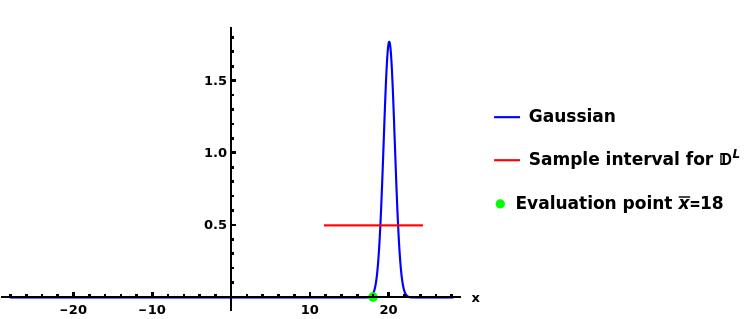
Figure 1: Gaussian function together with evaluation point $\bar{x}$, and sample interval used for calculating $\mathbb{D}^{L}(f)(\bar{x})$. $L=10^{5}$

In figure 2, we show the terms in the series defining the quantity $\mathbb{D}^{L}(f)(\bar{x})$. It is worth noting that for the given value of $L$, and an accuracy goal of $10^{-8}$ we need to include $10^{5}$ terms in our series. This is easy to handle numerically for the Gaussian, but for functions that decay slower than a Gaussian, and for larger values of $L$, and higher accuracy, the calculations quickly become very challenging. We will soon see examples of this.

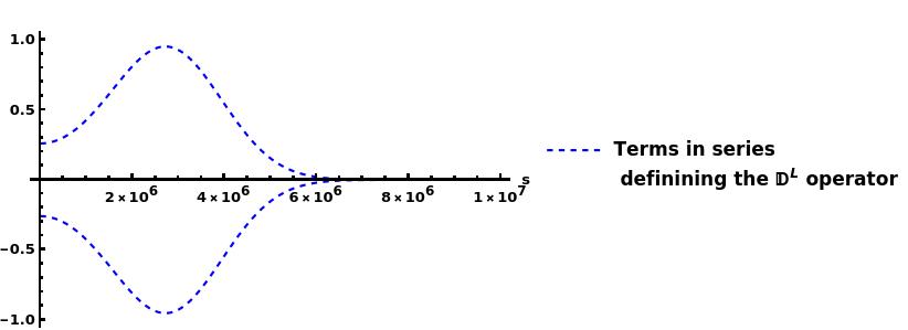
Figure 2: Sequence of terms in the infinite series defining the quantity $\mathbb{D}^{L}(f)(\bar{x})$ operator. $L=10^{5}$, accuracy goal $10^{-8}$.

In figure 3 we show the partial sums of the series for the quantity $\mathbb{D}^{L}(f)(\bar{x})$, where we sum the series from $s=1$, to $s=s_{*}$, for $s^{*}=1,\dots,s_{m}$. If the calculation is to converge, the graph in the figure needs to settle down for increasing values of $s_{*}$. We see that eventually it does, but that it actually grows for a large stretch of $s_{*}$ values. This is typical for what occurs while evaluating the $\mathbb{D}^{L}$ operator. The growth phase for the partial sums can stretch to very large values of $s_{*}$, and during this phase, the values of the partial sums can grow extremely large, until they eventually settle down. Handling this growth phase numerically in general requires arbitrary precision arithmetic.

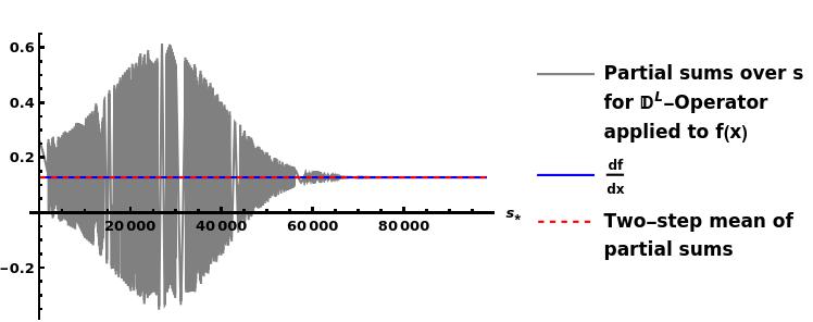
Figure 3: Partial sums of the infinite series defining the $\mathbb{D}^{L}$ operator. $L=10^{5}$

In the figure we also include the exact value for the derivative of $f$ in $x=\bar{x}$. This is the blue horizontal line in the figure. We observe that not only do the partial sums settle down, but they settle down to the exact value for the derivative. Or, to be precise, we find that the difference between $\mathbb{D}^{L}(f)(\bar{x})$ and $f^{\prime}(\bar{x})$ when $s_{*}=s_{m}$ is less than $10^{-8}$ which was the prescribed precision goal.

In the figure we also show a curve that represents the sliding mean of each pair of consecutive terms in the partial sums. This is the red dotted curve in the figure. This curve appears in the figure to coincide with the exact value for the derivative for essentially all the partial sums, starting with $s_{*}=2$. It seems to tell us that the non-locality of the $\mathbb{D}$ operator is perhaps only apparent; when evaluating the series determining $\mathbb{D}^{L}(f)(\bar{x})$, only the first few terms in the sum contribute to the final value, and that this final value comes from the remainder of the near-cancellation of the first few alternation terms. Consecutive terms, further out in the sum, are the non-local terms that sample values of the Gaussian far from $x=\bar{x}$, cancel up to a remainder that is too small to show up in the plot. This is however not the whole story.

In figure 4 we leave out the partial sums, retaining only the sliding mean of the partial sums, and the exact value of the derivative, this is now the red dotted curve. Zooming in on these two curves, we see that partial sums which sample values of the Gaussian far from the evaluation point do give a contribution to the value of $\mathbb{D}^{L}(f)(\bar{x})$. It is small, but these non-local contributions are needed in order to approximate the exact value $f^{\prime}(\bar{x})$ to the specified accuracy.

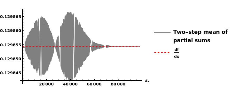
Figure 4: Two-step mean of the partial sums. $L=10^{5}$

Recall however that according to the conjecture, $\mathbb{D}^{L}(f)(\bar{x})$ only needs to coincide with $f^{\prime}(\bar{x})$ in the limit when $L$ approaches infinity. Thus, the fact that the figures show non-locality for $\mathbb{D}^{L}$ is not surprising.

In figures 5 and 6 we increase $L$ to the value $L=10^{7}$ and redo the calculations. The curves in the figures look very much the same as before, but in figure 6 we see that even if the non-locality appears to be about as extensive as for the smaller value of $L$ in figure 4, the size of the contribution of the non-local terms to the final sum is smaller.

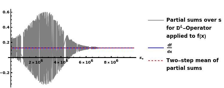
Figure 5: Partial sums of the infinite series defining the $\mathbb{D}^{L}$ operator; $L=10^{7}$

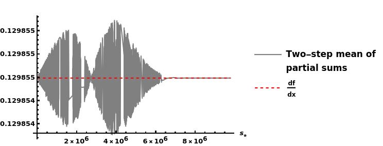
Figure 6: Two-step mean of the partial sums; ; $L=10^{7}$

One should of course not expect to be able to calculate $f^{\prime}(\bar{x})$ to arbitrary precision for fixed $L$ by including enough terms in the series defining $\mathbb{D}^{L}$.

Notwithstanding that, for a function as nice as a Gaussian we can for our chosen value of $L=10^{5}$, squeeze the difference between $\mathbb{D}^{L}(f)(\bar{x})$ and $f^{\prime}(\bar{x})$ down to at most $10^{-996}$, and no more. This accuracy is achieved by summing up $10^{6}$ terms in the sum. In order to reach this accuracy we did the calculations with a 1000 digit accuracy. This is of course a very high accuracy, and that it is achievable for the Gaussian after only summing up $10^{6}$ terms is most certainly dependent on the fact that the Gaussian decays exponentially away from its center point $x_{0}$. For functions that decay more slowly, like the Lorentzian function which we will discuss next, to find the achievable accuracy, for a fixed value of $L$, requires many more terms than for the Gaussian.

5.1.2 Lorentzian

For the Lorentzian

$$f(x)=\frac{1}{1+x^{2}},$$

we pick the point where we want to evaluate $\mathbb{D}^{L}(f)$ to be $\bar{x}=2$, and we let, as for the Gaussian, $L=10^{5}$. Furthermore, we seek the same accuracy goal as for the Gaussian, $10^{-8}$.

In figure 7 we show the Lorentzian, the evaluation point, and part of the sample interval. The actual sample interval was much larger and approximately given by $[-60,64]$.

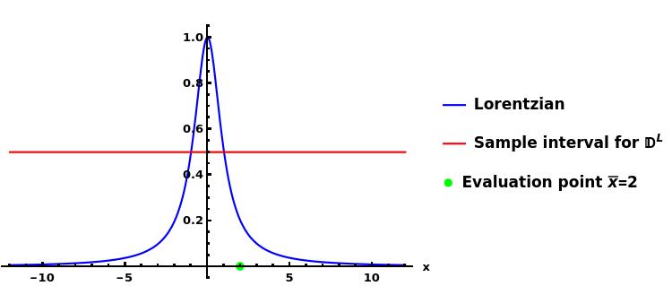
Figure 7: Lorentzian function together with evaluation point $\bar{x}$, and part of the sample interval used for calculating $\mathbb{D}^{L}(f)(\bar{x})$. $L=10^{5}$

The next two figures, 8 and 9, correspond to the figures, 5 and 6 for the Gaussian case. We observe that the quantity $\mathbb{D}^{L}(f)(\bar{x})$ behaves qualitatively very much like for the Gaussian case.

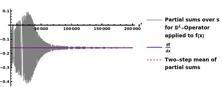
Figure 8: Partial sums of the infinite series defining the $\mathbb{D}^{L}$ operator. $L=10^{5}$

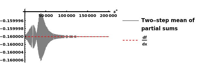
Figure 9: Two-step mean of the partial sums. $L=10^{5}$

For our fixed value of $L$, adding more terms in the series keeps increasing the accuracy, as in the Gaussian case, but for the Lorentzian the accuracy levels off at $10^{-1921}$ after summing $10^{550}$ terms.

Note that to achieve this kind of accuracy, we are not actually summing up the required $10^{550}$ terms, but rather are relying on well known methods that estimate the sum of alternating sums, without actually computing all the terms³.

5.1.3 Square root

For the square root

$$f(x)=\sqrt{x},\;\;x>0,$$

we pick the point where we want to evaluate $\mathbb{D}^{L}(f)$ to be $\bar{x}=1$, and we let the value of $L$, and the accuracy be the same as for the Gaussian and the Lorentzian.

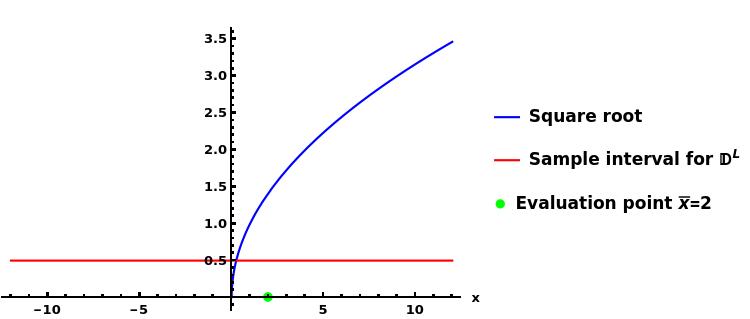
Figure 10: Square root function together with evaluation point $\bar{x}$, and part of the sample interval used for calculating $\mathbb{D}^{L}(f)(\bar{x})$. $L=10^{5}$

In figure 10 we show the square root, the evaluation point, and part of the sample interval. Like for the Lorentzian, the actual sample interval for the square root is much larger than shown. We find that for the accuracy we ask for, $10^{-8}$, the number of terms the series defining the quantity $\mathbb{D}^{L}(f)(\bar{x})$ is much too large to sum up directly. For example, summing up $10^{10}$ terms only give us the accuracy $10^{-2}$. In order to achieve the desired accuracy of $10^{-8}$, we must use the estimation methods like we did for the Lorentzian. If we do this we can achieve our desired accuracy of $10^{-8}$. The sampling interval we need for the square root in order to achieve this accuracy is enormous, and very much larger than for the Gaussian and the Lorentzian. This must surely be connected to the fact that the square root doesn’t decrease at all when $x$ grows, it actually increases.

Summing the series for the quantity $\mathbb{D}^{L}(f)(\bar{x})$, using the estimation method, we find that we need ca. $10^{20}$ terms in order to achieve an accuracy of $10^{-8}$. With respect to the achievable accuracy for the assumed value of $L$, we found that it is at least $10^{-55}$.

There is however an issue that arises while calculating $\mathbb{D}^{L}(f)(\bar{x})$ for the square root; the sample interval include negative $x$-values already for an accuracy of $10^{-8}$. For the computations we are doing in this paper, the square root function is defined to have a branch cut on the negative real axis. The values of the square root along the negative axis takes on purely imaginary values. So how come the quantity $\mathbb{D}^{L}(f)(\bar{x})$ is real? The only way this can occur is if all the imaginary parts in the series for the $\mathbb{D}^{L}$-operator cancel, up to the accuracy of the calculation. Computational investigations verify that this is indeed so. However, we don’t have a transparent mathematical explanation for why cancellation of all imaginary quantities takes place.

5.1.4 Tent function

For the tent function

$$f(x)=\left\{\begin{aligned} x+1,&\;\;\;-1\leq x\leq 0&\\ -x+1,&\;\;\;\;\;\;\;\;0\leq x\leq 1&\\ 0,&\;\;\;\;\;\;\;\;\;\absolutevalue{x}>1&\\ \end{aligned}\right.,$$

we pick the point where we want to evaluate $\mathbb{D}^{L}(f)$ to be $\bar{x}=-1/2$, and the same accuracy, $10^{-8}$ as the other examples above. In order to achieve this accuracy for the tent functions we need to increase the value of $L$ to $10^{7}$ and sum up ca. $10^{7}$ terms. Note that this $L$ is two orders of magnitude larger than the values of $L$ we needed for the Gaussian and Lorentzian cases.

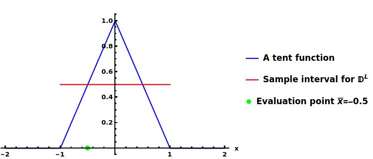
Figure 11: The tent function together with evaluation point $\bar{x}$, and the sample interval used for calculating $\mathbb{D}^{L}(f)(\bar{x})$. $L=10^{7}$

Figure 11,we shows the tent function, the chosen evaluation point, and the sample interval. Clearly, since the tent function has compact support, the sample interval can never be larger than the support. For the parameters we are using, the sample interval is as large as it can be, $[-1,1]$.

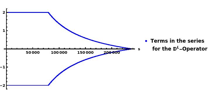
Figure 12: Sequence of terms in the infinite series defining the quantity $\mathbb{D}^{L}(f)(\bar{x})$, $L=10^{7}$, accuracy goal $10^{-8}$.

In figure 12 show the terms in the sequence defining the quantity $\mathbb{D}^{L}(f)(\bar{x})$, and in figure 13 we show the function $\mathbb{D}^{L}(f)(x)$. It is evident that $\mathbb{D}^{L}(f)(x)\approx f^{\prime}(x)$ for all $x$ where $f(x)$ is differentiable.

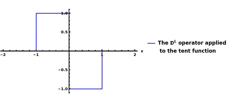
Figure 13: The function $\mathbb{D}^{L}(f)(x)$

Note that even if the tent function is not differentiable at the points ${-1,0,1}$, we can still try to apply the $\mathbb{D}^{L}$-operator to the tent function at these points. The numerical calculations we have done strongly indicate that

$$\mathbb{D}(f)(x)=\frac{1}{2}\left(\lim_{x->x^{+}}f^{\prime}(x)+\lim_{x->x^{-}}f^{\prime}(x)\right)=\{\frac{1}{2},0,-\frac{1}{2}\},\;\;\;\;\text{for}\;\;\;\;\;\;x\in\{-1,0,1\}.$$

5.1.5 Truncated ramp function

Here we explore the $\mathbb{D}$-operator for the case of discontinuous functions by introducing the following truncated ramp function

$$f(x)=\left\{\begin{aligned} 0,&\;\;\;\;\;\;\;\;x\leq-1&\\ x+1,&\;\;\;-1\leq x\leq 0&\\ 1-\frac{1-h}{l}x,&\;\;\;\;\;\;\;\;0\leq x<l&\\ 0,&\;\;\;\;\;\;\;\;\;x\geq l&\\ \end{aligned}\right.,$$

The function is continuous everywhere, except at the point $x=l$, and is continuously differentiable everywhere else, except for $x=-1,0,l$. The size of the drop at the point of discontinuity is given by $h$.

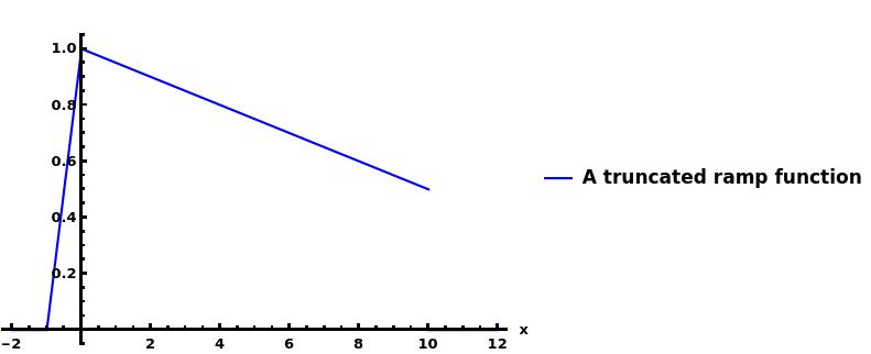
Figure 14: The truncated ramp function for $h=0.5$, and $l=10$.

Figure 14 is a graph of the truncated ramp function for the case $l=10$, and $h=0.5$. The function has compact support, and a formula for sum of the series determining $\mathbb{D}^{L}(f)(\bar{x})$ can be found. In figures 15 and 16 we use this formula to plot, for increasing value of $L$, $\mathbb{D}^{L}(f)(\bar{x})$, with $\bar{x}=-0.67$. At this point we have $f^{\prime}(\bar{x})=1$.

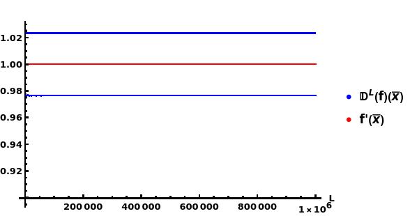
Figure 15: $\mathbb{D}^{L}(f)(\bar{x})$ for increasing value of $L$,together with the derivative of the truncated ramp function for the case $\bar{x}=-0.67$, $h=0.5$, and $l=10$

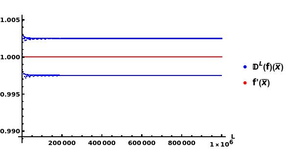
Figure 16: Same as figure 18, but now for $l=100$

These two figures tell us that as the distance between where we want to compute $\mathbb{D}(f)(\bar{x})$, and the point of discontinuity, increases, the fluctuating value of $\mathbb{D}^{L}(f)(\bar{x})$ gets ever closer to the exact value of the derivative $f^{\prime}(\bar{x})$. However, as far as we can tell from our numerics, no matter how far away from $x=\bar{x}$ the point of discontinuity is, the fluctuating values of $\mathbb{D}^{L}(f)(\bar{x})$ never settle down, and thus $\mathbb{D}(f)(\bar{x})$ does not exist.

Keeping $l$ fixed, but reducing the size of the drop at the point of discontinuity leads to the same behavior for the fluctuating values of $\mathbb{D}^{L}(f)(\bar{x})$. Thus no matter how small the drop at the discontinuity is, $\mathbb{D}(f)(\bar{x})$ does not exist.

5.1.6 Hat function

In this subsection we introduce the following hat function

$$f(x)=\left\{\begin{aligned} 0,&\;\;\;\;\;\;\;\;x\leq 0&\\ 1,&\;\;\;\;\;\;\;\;0<x<l&\\ 0,&\;\;\;\;\;\;\;\;\;x\geq 0&\\ \end{aligned}\right.,$$

where $l>0$.

For this simple function we can also find an exact formula for the quantity $\mathbb{D}^{L}(f)(\bar{x})$. The hat function, which is clearly discontinuous, reinforces the insight we got from the previous subsection with respect to the behavior of the quantity $\mathbb{D}^{L}(f)(\bar{x})$ for increasing $L$.

If we let the evaluation point be $\bar{x}=\frac{l}{2}-1$, the distance between the evaluation point and both points of discontinuity increases when $l$ increases. At this point we have $f^{\prime}(\bar{x})=0$.

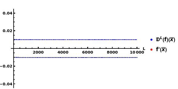
Figure 17: The sequence $\mathbb{D}^{L}(f)(\frac{l}{2}-1)$ for $l=20$, and increasing $L$ in the range $1\leq L\leq 10^{4}$.

In figure 17 we plot the sequence $\mathbb{D}^{L}(f)(\bar{x})$ for increasing values of $L$ in the range $1\leq L\leq 10^{3}$. The value of the sequence fluctuates around the correct value of the derivative. The amplitude of the fluctuations are on the order of $10^{-2}$.

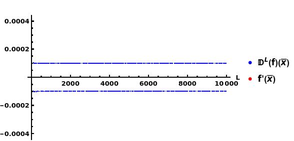
Figure 18: The same as in figure 17, but now $l=200$.

In figure 18 we increase $l$ to the value $l=200$ while keeping the evaluation point fixed. The evaluation point is now further from the two points of discontinuity than in figure 17. We see that the sequence $\mathbb{D}^{L}(f)(\bar{x})$ for increasing $L$ fluctuate around the correct value of the derivative, but the amplitude of the fluctuations are now of order $10^{-4}$.

From the formula it is easy to verify that for the symmetrically placed point $\bar{x}=\frac{l}{2}$, we find $\mathbb{D}(f)(\bar{x})=f^{\prime}(\bar{x})=0$. Thus, for this symmetrically placed point the conjecture holds.

Based on this and more numerical calculations, for other discontinuous functions, that we don’t show here, we conjecture that we will get similar results for any function that is discontinuous at one or more points. Thus, it does not matter how smooth it is away from the points of discontinuity, the mere presence of a discontinuity, anywhere, will in general invalidate our original conjecture (52), except perhaps for some special symmetrically placed points where the influence from the points of discontinuity cancel.

One could say that the existence of discontinuities unmask the apparent locality of the $\mathbb{D}$-operator we have seen while applying it to smooth functions.

The numerical calculations in this section, together with many more that we are not reporting here, strongly indicate that our original conjecture (52) is true for many, perhaps most functions. However, approximate numerical calculations, even if the accuracy is very high, are not a substitute for exact analytical calculations and mathematical proofs.

This is of course a truism, but for the particular case of the $\mathbb{D}^{L}$ operator, it is still worth stressing. The reason being that the numerical calculations of this operator sometimes involve trying to sum an astronomical number of terms, in a series where consecutive terms cancel to a very high accuracy. Without using arbitrary precision arithmetic, the calculation of the $\mathbb{D}^{L}$-operator would not be possible. For the most part, the calculations would also fail if we did not use methods that estimate the sum, without actually summing the, sometimes, impossibly large number of terms involved.

All of the above make it of paramount importance to seek exact results in terms of analytic summation of the series for special functions, and mathematical proofs for sizable classes of functions. In the following sections we will do both.

5.2 Analytical evidence in support of the conjecture

In this subsection we are going to prove that

$$\mathbb{D}(e^{ikx})=ike^{ikx}.$$ (53)

Observe that

$$\mathbb{D}(e^{ikx}) =\lim_{L\rightarrow\infty}\sum_{s=1}^{\infty}(-1)^{(s-1)}\frac{e^{ik(x+\triangle s)}-e^{ik(x-\triangle s)}}{\triangle s}$$

$$=e^{ikx}\lim_{L\rightarrow\infty}\sum_{s=1}^{\infty}(-1)^{(s-1)}\frac{e^{ik\triangle s}-e^{-ik\triangle s}}{\triangle s}$$

$$=2ike^{ikx}\lim_{L\rightarrow\infty}\sum_{s=1}^{\infty}(-1)^{(s-1)}\frac{\sin{k\triangle s}}{k\triangle s}.$$

In order for (53) to be true, we must have

$$\lim_{L\rightarrow\infty}\sum_{s=1}^{\infty}(-1)^{(s-1)}\operatorname{sinc}{k\triangle s}=\frac{1}{2}.$$ (54)

We will now show that (54) does in fact hold.

Introducing the function $\operatorname{sinc}{x}=\frac{sin{x}}{x}$, which is a function well known from signal analysis and the theory of the Fourier transform, we evidently have

$$\sum_{s=1}^{\infty}(-1)^{(s-1)}\operatorname{sinc}{k\triangle s}$$

$$=\sum_{p=1}^{\infty}\operatorname{sinc}{k\triangle(2p+1)}-\sum_{p=1}^{\infty}\operatorname{sinc}{k\triangle 2p}.$$ (55)

Both series in (55) can be summed exactly, using for example the symbolic computing system Mathematica. We have

$$\sum_{s=1}^{\infty}(-1)^{(s-1)}\operatorname{sinc}{k\triangle s}=$$

$$\left(\frac{i}{4\triangle k}\right)\Big{\{}-\log\left(1-e^{-i\triangle k}\right)+\log\left(1+e^{-i\triangle k}\right)+\log\left(1-e^{-2i\triangle k}\right)$$

$$+\log\left(1-e^{i\triangle k}\right)-\log\left(1+e^{i\triangle k}\right)-\log\left(1-e^{2i\triangle k}\right)\Big{\}}$$

$$=\left(\frac{1}{2\triangle k}\right)\Big{\{}\text{Arg}(1+e^{i\triangle k})+\text{Arg}(1-e^{2i\triangle k})-\text{Arg}(1-e^{i\triangle k})\Big{\}},$$ (56)

where we have used the definition of the complex logarithm and where Arg is the principal argument function with values in the interval $(-\pi,\pi]$.

We are only interested in the expression (56) in the limit when $L$ approach infinity. This corresponds to $\triangle$ approaching zero.

In this limit, the second term in (56) takes the asymptotic form

$$\text{Arg}(1-e^{2i\triangle k}) \approx-\text{Arg}\left(-\frac{(\triangle k)^{4}}{24}+\frac{i(\triangle k)^{3}}{6}+\frac{(\triangle k)^{2}}{2}-i\triangle k\right)$$

$$\approx-\tan^{-1}\left(\frac{1}{\triangle k}-\frac{\triangle k}{6}\right).$$ (57)

In a similar way, we find that the third term in (56) takes the asymptotic form

$$\text{Arg}(1-e^{i\triangle k}) \approx-\tan^{-1}\left(\frac{2}{\triangle k}-\frac{\triangle k}{6}\right).$$ (58)

Note that in each of formulas (57) and (58) there are troublesome terms that approach infinity when $\triangle$ approach zero. However, note also that in the expression (56) the third term is subtracted from the the second term.

Using the trigonometric identity

$$\tan^{-1}a-\tan^{-1}b=\tan^{-1}\left(\frac{a-b}{1+ab}\right),$$

we find that

$$\text{Arg}(1-e^{2i\triangle k})-\text{Arg}(1-e^{i\triangle k})\approx\frac{\tan^{-1}\left(\frac{\triangle k}{2}\right)}{2\triangle k}.$$

The asymptotic expression for the first term in (56) does not contain any troublesome terms that approach infinity and is simply

$$\text{Arg}(1+e^{i\triangle k})\approx\frac{\tan^{-1}\left(\frac{\triangle k}{2}\right)}{2\triangle k}.$$

Thus we finally have

$$\sum_{s=1}^{\infty}(-1)^{(s-1)}\operatorname{sinc}{k\triangle s}\approx\frac{\tan^{-1}\left(\frac{\triangle k}{2}\right)}{\triangle k}\approx\frac{1}{2},$$

which shows that in the limit when $L\rightarrow\infty$, the identity (54) does indeed hold.

Using the results proven above we can immediately conclude that

Proposition 1.

Let

$$a_{-N},a_{-N+1},\cdots,a_{N-1},a_{N},$$

be a set of $2N+1$ complex numbers, and let

$$k_{n}=\frac{2\pi n}{L},\;n=-N,\cdots,N.$$

Then the conjecture is true for the function

$$f(x)=\sum_{n=-N}^{N}\;a_{n}e^{ik_{n}x}.$$

It is well known that functions of the type described in the proposition can approximate any function of period $L$, arbitrarily well.

5.3 Proving the conjecture

Recall that the conjecture, as stated, is

$$\mathbb{D}(f)(x)=f^{\prime}(x).$$

In the following we will assume the the functions referred to in the conjecture are real valued and defined on the whole of $\mathbb{R}$.

Let us start by rewriting the $\mathbb{D}$ operator in the following way

$$\mathbb{D}(f)(x_{0}) =\lim_{L\rightarrow\infty}\;\sum_{s=1}^{\infty}(-1)^{(s-1)}\frac{f(x_{0}+\triangle s)-f(x_{0}-\triangle s)}{\triangle s}$$

$$=\lim_{\triangle\rightarrow 0}\;\sum_{s\neq 0}(-1)^{(s-1)}\frac{f(x_{0}+\triangle s)}{\triangle s}$$

$$=\lim_{\triangle\rightarrow 0}\;\left\{\left(\sum_{s\neq 0}(-1)^{(s-1)}\frac{\delta(x-x_{0}-\triangle s)}{\triangle s}\right)(f)\right\}$$

$$=\lim_{\triangle\rightarrow 0}\;\left\{\mathbf{\mathcal{D}}(x-x_{0})(f)\right\},$$ (59)

where we have used the fact that $\triangle=\frac{2\pi}{L}$, and where we have defined a distribution

$$\mathbf{\mathcal{D}}(x-x_{0})=\sum_{s\neq 0}(-1)^{(s-1)}\frac{\delta(x-x_{0}-\triangle s)}{\triangle s}.$$ (60)

Next, observe that if ${\operatorname{comb}}$ is the Dirac comb distribution, we have

$$\left(-\left(\frac{1}{\triangle}\operatorname{sinc}{\left(\frac{x-x_{0}}{\triangle}\right)}\right)^{\prime}\operatorname{comb}{\left(\frac{x-x_{0}}{\triangle}\right)}\right)$$

$$=-\frac{1}{\triangle^{2}}\operatorname{sinc}^{\prime}{\left(\frac{x-x_{0}}{\triangle}\right)}\operatorname{comb}{\left(\frac{x-x_{0}}{\triangle}\right)}$$

$$=-\frac{1}{\triangle^{2}}\left(\frac{\cos\pi\left(\frac{x-x_{0}}{\triangle}\right)}{\frac{x-x_{0}}{\triangle}}-\frac{\sin\pi\left(\frac{x-x_{0}}{\triangle}\right)}{\pi\left(\frac{x-x_{0}}{\triangle}\right)^{2}}\right)\operatorname{comb}{\left(\frac{x-x_{0}}{\triangle}\right)}$$

$$=-\frac{1}{\triangle^{2}}\sum_{s\neq 0}\left(\frac{\cos s\pi}{s}-\frac{\sin s\pi}{\pi s^{2}}\right)\delta\left(\frac{x-x_{0}}{\triangle}-s\right)$$

$$=\sum_{s\neq 0}(-1)^{s-1}\frac{\delta\left(\frac{x-x_{0}}{\triangle}-s\right)}{s\triangle^{2}}$$

$$=\sum_{s\neq 0}(-1)^{s-1}\frac{\delta\left(x-x_{0}-\triangle s\right)}{s\triangle},$$ (61)

where we have made use of the fact that

$$\frac{\cos x\pi}{x}-\frac{\sin x\pi}{\pi x^{2}}\rightarrow 0,\;\text{when}\;x\rightarrow 0.$$

Using (60) and (61) we see that the distribution $\mathbf{\mathcal{D}}(x-x_{0})$ can be written in the form

$$\mathbf{\mathcal{D}}(x-x_{0})=-\left(\frac{1}{\triangle}\operatorname{sinc}{\left(\frac{x-x_{0}}{\triangle}\right)}\right)^{\prime}\operatorname{comb}{\left(\frac{x-x_{0}}{\triangle}\right)}.$$ (62)

We are now going to compute the Fourier transform of the distribution (62). For that purpose we note that in this paper we are using the following convention for the Fourier transform

$$F(k) =\frac{1}{\sqrt{2\pi}}\int_{-\infty}^{\infty}dx\;f(x)\;e^{ikx},$$

$$f(x) =\frac{1}{\sqrt{2\pi}}\int_{-\infty}^{\infty}dk\;F(k)\;e^{-ikx}.$$ (63)

Using this convention, we have for any function, or distribution, f,

$$f\left(\frac{x-x_{0}}{\triangle}\right)\; \rightarrow\;\triangle e^{ikx_{0}}\;F(\triangle k),$$

$$f^{\prime}\left(\frac{x-x_{0}}{\triangle}\right)\; \rightarrow\;-ik\triangle^{2}e^{ikx_{0}}\;F(\triangle k).$$

Note that with our convention (63), the Fourier transform of the Dirac $\operatorname{comb}$ is not equal to itself. We rather have

$$\operatorname{comb}(x)\rightarrow\frac{1}{\sqrt{2\pi}}\operatorname{comb}(k).$$

From these simple facts we have

$$\mathbf{\mathcal{D}}(x-x_{0}) \rightarrow-\left(\frac{1}{\triangle^{2}}\right)\left(-ik\triangle^{2}e^{ikx_{0}}\;\operatorname{rect}(\triangle k)\right)*\left(\frac{\triangle}{\sqrt{2\pi}}e^{ikx_{0}}\;\operatorname{comb}(\triangle k)\right)$$

$$=\left(ike^{ikx_{0}}\operatorname{rect}(\triangle k)\right)*\left(\frac{\triangle}{\sqrt{2\pi}}e^{ikx_{0}}\operatorname{comb}(\triangle k)\right)$$

$$=\frac{i}{\sqrt{2\pi}}e^{ikx_{0}}\sum_{s=-\infty}^{\infty}(k-\frac{s}{\triangle})\operatorname{rect}(\triangle k-s),$$ (64)

where we have used the fact that the Fourier transform of the $\operatorname{sinc}$ function is a rectangle

$$\operatorname{rect}(k)=\left\{\begin{aligned} 1,\;\;\;\absolutevalue{k}\leq\frac{1}{2}\\ 0.\;\;\;\absolutevalue{k}>\frac{1}{2}\\ \end{aligned}\right..$$

The Fourier transform of $\mathbf{\mathcal{D}}(x-x_{0})$ takes for $x_{0}=0$ the form of a periodic piecewise linear function of slope equal one, and period $\frac{1}{\triangle}$. A classical saw tooth function.

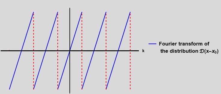
Figure 19: The real part of the Fourier transform of $\mathbf{\mathcal{D}}(x-x_{0})$ for $x_{0}=0$ and $\triangle=1$.

Using our convention for the Fourier transform, it is a simple matter to verify that the Fourier transform of the distribution $-\delta^{\prime}(x-x_{0})$ is given by

$$-\delta^{\prime}(x-x_{0})\rightarrow\frac{ik}{\sqrt{2\pi}}e^{ikx_{0}}.$$ (65)

Now, from (59) we have for the Fourier transform of $\mathbb{D}(f)(x_{0})$,

$$\mathbb{D}(f)(x_{0}) \rightarrow\lim_{\triangle\rightarrow 0}\;\left\{\left(\frac{i}{\sqrt{2\pi}}e^{ikx_{0}}\sum_{s=-\infty}^{\infty}(k-\frac{s}{\triangle})\operatorname{rect}(\triangle k-s)\right)(F)\right\}$$

$$=\lim_{\triangle\rightarrow 0}\;\left\{\int_{-\infty}^{\infty}dk\;F(k)\frac{i}{\sqrt{2\pi}}e^{ikx_{0}}\sum_{s=-\infty}^{\infty}(k-\frac{s}{\triangle})\operatorname{rect}(\triangle k-s)\right\}$$ (66)

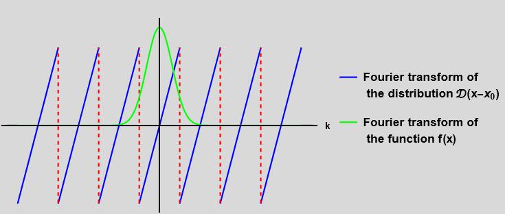
Figure 20: The real part of the integrand from formula (66) for the case when $\triangle=1$, $x_{0}=0$ and the Fourier transform of f(x) is a Gaussian centered at $k=0$

Observe that when we take the limit when $\triangle\rightarrow 0$, the first period of the periodic piecewise linear function (64), which is displayed in figure 19, will grow without bound.

From this observation, together with identity (65) and figure 20, we can now immediately conclude that

Proposition 2.

The conjecture is true for any function f(x) whose Fourier transform has compact support.

Thus, compact support for the Fourier transform of a function $f(x)$ is a sufficient condition for the truth of the statement

$$D(f)(x)=f^{\prime}(x).$$

This sufficient condition is however very strong, most of our numerical evidence concerns itself with functions whose Fourier transform does not have compact support. It is well known that functions whose Fourier transform has compact support are in fact analytic.

We will next show that the conjecture is also true for functions whose Fourier transform does not have compact support, but rather decay sufficiently fast for large $k$. In order to show this we rewrite (66) in the following way

$$\mathbb{D}(f)(x_{0}) \rightarrow\lim_{\triangle\rightarrow 0}\;\left\{\int_{-\infty}^{\infty}dk\;F(k)\frac{i}{\sqrt{2\pi}}e^{ikx_{0}}\sum_{s=-\infty}^{\infty}(k-\frac{s}{\triangle})\operatorname{rect}(\triangle k-s)\right\}$$

$$=\lim_{\triangle\rightarrow 0}\;\int_{-\infty}^{\infty}dk\;F(k)\frac{ik}{\sqrt{2\pi}}e^{ikx_{0}}\sum_{s=-\infty}^{\infty}\operatorname{rect}(\triangle k-s)$$

$$-\lim_{\triangle\rightarrow 0}\;\int_{-\infty}^{\infty}dk\;F(k)\frac{i}{\sqrt{2\pi}}e^{ikx_{0}}\sum_{s=-\infty}^{\infty}\frac{s}{\triangle}\operatorname{rect}(\triangle k-s)$$

$$=\int_{-\infty}^{\infty}dk\;F(k)\frac{ik}{\sqrt{2\pi}}e^{ikx_{0}}$$

$$-\lim_{\triangle\rightarrow 0}\;\frac{i}{\sqrt{2\pi}}\sum_{s=-\infty}^{\infty}\int_{-\infty}^{\infty}dk\;F(k)e^{ikx_{0}}\frac{s}{\triangle}\operatorname{rect}(\triangle k-s).$$ (67)

The first term in (67) is according to (65) the Fourier transform of the distribution $-\delta^{\prime}(x-x_{0})$ applied to the Fourier transform, $F(k)$, of our function $f(x)$. Thus, if the second term in (67) is zero, we can conclude that

$$D(f)(x_{0})=-\delta^{\prime}(x-x_{0})(f).$$ (68)

Thus, the conjecture is true for functions for which the second term in (67) is exactly zero.

Observe that

$$\frac{i}{\sqrt{2\pi}}\sum_{s=-\infty}^{-1}\int_{-\infty}^{\infty}dk\;F(k)e^{ikx_{0}}\frac{s}{\triangle}\operatorname{rect}(\triangle k-s)$$

$$=-\frac{i}{\sqrt{2\pi}}\sum_{s=1}^{\infty}\int_{-\infty}^{\infty}dk\;F(k)e^{ikx_{0}}\frac{s}{\triangle}\operatorname{rect}(\triangle k+s))$$

$$=-\frac{i}{\sqrt{2\pi}}\sum_{s=1}^{\infty}\int_{-\infty}^{\infty}dk\;F(-k)e^{-ikx_{0}}\frac{s}{\triangle}\operatorname{rect}(-\triangle k+s))$$

$$=-\frac{i}{\sqrt{2\pi}}\sum_{s=1}^{\infty}\int_{-\infty}^{\infty}dk\;F(k)^{*}e^{-ikx_{0}}\frac{s}{\triangle}\operatorname{rect}(\triangle k-s))$$

$$=\left\{\frac{i}{\sqrt{2\pi}}\sum_{s=1}^{\infty}\int_{-\infty}^{\infty}dk\;F(k)e^{ikx_{0}}\frac{s}{\triangle}\operatorname{rect}(\triangle k-s))\right\}^{*}.$$ (69)

From (69), (67), the definition of convergence for a doubly infinite series, and the discussion above leading up to (68), we can now conclude that

Lemma 1.

Let $f(x)$ be a function whose Fourier transform is a function, $F(k)$. Then the conjecture is true for $f(x)$, at $x=x_{0}$, if and only if

$$\lim_{\triangle\rightarrow 0}\;S(x_{0},\triangle)=0,$$

where

$$S(x_{0},\triangle)=\sum_{s=1}^{\infty}\frac{s}{\triangle}\int_{\frac{s-\frac{1}{2}}{\triangle}}^{\frac{s+\frac{1}{2}}{\triangle}}dk\;F(k)e^{ikx_{0}}.$$

This lemma tells us exactly what we need to do to verify that the conjecture is true for any particular $f(x)$.

Let us for example assume that the Fourier transform of $f(x)$, $F(k)$, has a bound

$$\absolutevalue{F(k)}\leq\alpha\;s^{-\gamma},\;\;\text{where}\;\;\gamma>2.$$

Given this, we have

$$\absolutevalue{S(x_{0},\triangle)} \leq\alpha\sum_{s=1}^{\infty}\frac{s}{\triangle}\int_{\frac{s-\frac{1}{2}}{\triangle}}^{\frac{s+\frac{1}{2}}{\triangle}}dk\;k^{-\gamma}$$

$$=\frac{\alpha}{\gamma-1}\sum_{s=1}^{\infty}\frac{s}{\triangle}\left(\left(\frac{s-\frac{1}{2}}{\triangle}\right)^{1-\gamma}-\left(\frac{s+\frac{1}{2}}{\triangle}\right)^{1-\gamma}\right)$$

$$=\frac{\alpha\triangle^{\gamma-2}}{\gamma-1}\sum_{s=1}^{\infty}s\left(\left(s-\frac{1}{2}\right)^{1-\gamma}-\left(s+\frac{1}{2}\right)^{1-\gamma}\right),$$ (70)

and since

$$s\left(\left(s-\frac{1}{2}\right)^{1-\gamma}-\left(s+\frac{1}{2}\right)^{1-\gamma}\right)\sim(\gamma-1)\;s^{-(\gamma-1)},\;\;\;\text{when}\;\;s\rightarrow\infty,$$

the infinite series in (70) converges. Given this, and the assumption that $\gamma>2$, it is now evident that

$$\lim_{\triangle\rightarrow 0}\;S(x_{0},\triangle)=0.$$

Thus we have

Theorem 1.

Let $f(x)$ be a function whose Fourier transform, $F(k)$, satisfies the bound

$$\absolutevalue{F(k)}\leq\alpha\;k^{-\gamma},\;\;\;\text{for}\;k>c,$$

for some numbers $\alpha>0,c>0$, and $\gamma>2$.

Then

$$\mathbb{D}(f)(x)=f^{\prime}(x),\;\;\;\text{for all}\;x\in\mathbb{R}$$

Note that the required bound on the Fourier transform in the theorem does hold for the shifted Gaussian and the Lorentzian, but does not hold for the square root, and the triangle function, for which our numerics indicate strongly that the conjecture is true. Thus, theorem 1 is fine, as far as it goes, but is certainly not the final word with respect to the truth of the conjecture.

5.4 Complex functions

In this section we generalize the $\mathbb{D}$ operator to an operator on functions, $f(z)$, of a complex variable. The formula for the operator is

$$\mathbb{D}_{\xi}(f)(z)=\lim_{L\rightarrow\infty}\sum_{s=1}^{\infty}(-1)^{(s-1)}\frac{f(z+\xi\triangle s)-f(z-\xi\triangle s)}{\xi\triangle s},$$

where $\xi$ is a complex number of unit length, $\absolutevalue{\xi}=1$. Thus for the operator $\mathbb{D}_{\xi}$ our sampling occur along a straight line in the complex plane. The direction of the line is determined by the complex number $\xi$.

Let us consider the complex function

$$f(z)=\arcsin(z).$$

Let us pick the point where we want to evaluate $\mathbb{D}_{\xi}(f)$ to be $\bar{z}=0.5i$, let $L=10^{4}$, the accuracy be $10^{-6}$, and let $\xi=\frac{1}{\sqrt{2}}(1+i)$. In figure 21 we show a plot of the complex argument of $f(z)$, together with the evaluation point and a small section of the sample line. The branch cuts for the function are marked with gray.

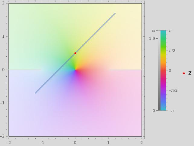
Figure 21: Plot of argument of the $\arcsin$, together with the evaluation point $\bar{z}$ and part of the sample line. The branch cuts are displayed in gray.

We find that in order to achieve the desired accuracy we need to include $10^{10}$ terms in the series defining the quantity $\mathbb{D}_{\xi}(f)(\bar{z})$. This is the highest accuracy we can reach in a reasonable time while directly summing up the terms in the series. Summing up the series using estimation methods, we find that using $10^{20}$ terms in the series, and calculating with $25$ digits accuracy, $\mathbb{D}_{\xi}(f)(\bar{z})=f^{\prime}(z)$ within machine precision.

We have also observed using numerical computations that the quantity $\mathbb{D}_{\xi}(f)(\bar{z})$ does not appear to depend on $\xi$, meaning that the quantity is independent on which sample line, through the point $\bar{z}$, we use. Since $f(z)=\arcsin(z)$ is analytic at the point $\bar{z}=0.5i$, this is perhaps not so unexpected. If our $\mathbb{D}_{\xi}$ operator is equal to the complex derivative, this is of course exactly what would have to happen. On the same theme, we find that if we apply our operator to a complex function that is not analytic, for example $f(z)=\absolutevalue{z}$, then the quantity $\mathbb{D}_{\xi}(f)(z)$ does depend on the direction of the sample line.

We have done investigations like the above for several different functions of a complex variable, and all these cases support the complex version of the original conjecture (52),

$$\mathbb{D}_{\xi}(f)(\bar{z})=\frac{df}{dz}(\bar{z}),$$

independently of $\xi$, if $f$ is analytic in $z=\bar{z}$.

Our original conjecture, which was inspired by deriving the continuum limit of the total angular momentum of a scalar field in a square cavity, was restricted to functions defined on the real axis. The sample line was also restricted to being located on the real axis. However, if a function on the real axis can be extended to complex variables, one can apply the extended $\mathbb{D}_{\xi}$ operator discussed in this section to compute $\mathbb{D}_{\xi}(f)(x)$ for x on the real line, where the sample line now is in the complex plane. We have investigated several such situations where the extended function is analytic in a domain containing the real axis. In all such cases we find that

$$\mathbb{D}_{\xi}(f)(x)=\mathbb{D}(f)(x),$$

independently of $\xi$. Thus, $\mathbb{D}_{\xi}$ is truly an extension of $\mathbb{D}$.

6 Acknowledgment

The authors are thankful for support from the Department of mathematics and statistics at the Arctic University of Norway, from the Arizona Center for Mathematical Sciences at the University of Arizona, and for the support from the Air Force Office for Scientific Research under Grant No. FA9550-19-1-0032. The authors are also thankful for very insightful discussions and very constructive critique of the ideas appearing in the paper from Miro Kolesik at the Wyant College of Optical Sciences, Arizona, USA.

References

- 1 C. G. Darwin, “Notes on the Theory of Radiation,” Proc. Roy. Soc. London A 136, 36-52 (1932).
- 2 D. S. Jones, ”The theory of electromagnetism”, page 14, Pergamon Press, (1964).
- 3 Wolfram Research (1988), NSum, Wolfram Language function, https://reference.wolfram.com/language/ref/NSum.html (updated 2007).
- 4 C. Cohen-Tannoudji, J. Dupont-Roc, and G. Grynberg, Photons and Atoms: Introduction to Quantum Electrodynamics, Wiley, New York (1989). See complement BI, Eq.(11).
- 5 H. A. Haus and J. L. Pan, “Photon spin and the paraxial wave equation,” Am. J. Phys. 61, 818-821 (1993).
- 6 S. Weinberg, ”The quantum theory of fields”, Volume 1, page 306, Cambridge, (1995).
- 7 J.D. Jackson,Classical Electrodynamics (3rd edition), Wiley, New York (1999).
- 8 S. M. Barnett, “Optical angular-momentum flux,” J. Opt. B: Quantum Semiclassical Optics 4, S7-16 (2002).
- 9 L. Allen, S. M. Barnett, and M. J. Padgett,” Optical Angular Momentum”, Institute of Physics Publishing, Bristol, United Kingdom (2003).
- 10 G. Grynberg, A. Aspect, and C. Fabre,Introduction to Quantum Optics, Cambridge University Press, Cambridge, United Kingdom (2010).
- 11 S. M. Barnett, “Rotation of electromagnetic fields and the nature of optical angular momentum,” J. Mod. Opt. 57, 1339-1343 (2010).
- 12 M. Mansuripur,“Spin and orbital angular momenta of electromagnetic waves in free space,”Physical Review A 84, 033838 (2011)
- 13 L. Marrucci, E. Karimi, S. Slussarenko, B. Piccirillo, E. Santamato, E. Nagali, and F. Sciarrino, “Spin-to-orbital conversion of the angular momentum of light and its classical and quantum applications,” J. Opt. 13, 064001 (2011).
- 14 I. Bialynicki-Birula and Z. Bialynicka-Birula, “Canonical separation of angular momentum of light into its orbital and spin parts,” arXive:1105.5728v1 [quant-ph] 28 May 2011.
- 15 P. K. Jakobsen, ”Topics in applied Mathematics and nonlinear waves”, (2019), doi.org/10.48550/arXiv.1904.07702.
- 16 M. Mansuripur, “Spin and orbital angular momenta of electromagnetic waves in classical and quantum electro-dynamics,” Proceedings of SPIE 12656, Spintronics XVI 1265604 (2023); doi: 10.1117/12.2675779.
- 17 M. Mansuripur, “Electromagnetic angular momentum of quantized wavepackets in free space,” Proceedings of SPIE 12649, Optical Trapping and Optical Micromanipulation XX, 126490A (2023); doi: 10.1117/12.2675775