Dynamic Regret and Cumulative Constraint Violation Analysis for Distributed Online Constrained Convex Optimization
with Event-Triggered Communication

Abstract

This paper focuses on the distributed online convex optimization problem with time-varying inequality constraints over a network of agents, where each agent collaborates with its neighboring agents to minimize the cumulative network-wide loss over time. To reduce communication overhead between the agents, we propose a distributed event-triggered online primal–dual algorithm over a time-varying directed graph. Dynamic network regret and network cumulative constraint violation are leveraged to measure the performance of the algorithm. Based on the natural decreasing parameter sequences, we establish sublinear dynamic network regret and network cumulative constraint violation bounds. The theoretical results broaden the applicability of event-triggered online convex optimization to the regime with inequality constraints. Finally, a numerical simulation example is provided to verify the theoretical results.

I INTRODUCTION

Distributed optimization has wide applications in sensor networks [1], machine learning [2] and power systems [3], where a network of agents aims at minimizing the average of all the local cost functions by exchanging local information of the agents. It can be traced back at least to [4, 5]. The past decades have witnessed the rapid development of the classical distributed optimization, see recent survey papers [6, 7, 8]. However, the local loss functions are static over time, which may not be applicable to dynamic and uncertain environments[9].

Distributed online convex optimization is a promising framework due to its powerful modeling capability for many problems in dynamic, uncertain and even adversarial environments. In distributed online convex optimization, the agents collaboratively make decisions without knowing their local loss functions at the current iteration, and then the time-varying local loss functions are privately revealed. The goal is to minimize the cumulative network-wide loss over time. In general, static regret is the standard performance metric to evaluate the online algorithms, which measures the difference of the cumulative loss between the decision sequence and the best fixed decision in hindsight. Various distributed online algorithms have been developed in recent years, and the decision sequence of each agent induced by the online algorithms achieves sublinear static regret, see [10, 11, 12, 13, 14, 15, 16, 17, 18, 19], recent survey paper [20] and references herein. To name a few, the authors of [10] develop a projection-based distributed online subgradient descent algorithm to avoid sharing sensitive information and storing information in a central location such that online convex optimization has intrinsic privacy-preserving properties. Using Bregman divergence in lieu of Euclidean distance for projection, the authors of [11] propose a decentralized online mirror descent algorithm to deal with large-scale optimization.

In the literature, most of existing distributed online algorithms at each iteration require local information exchange between the agents via the underlying communication network, which may cause tremendous communication overhead in many practical applications, e.g., large-scale multi-agent systems and sensor networks with small battery capacity. To tackle this challenge, the authors of [21] introduce event-triggered communication to the algorithm in [10] and then propose two event-triggered algorithms with full-information feedback and bandit feedback over a fixed graph, respectively. Moreover, sublinear static regret is achieved for the two event-triggered algorithms when their event-triggering threshold sequences are non-increasing and converge to zero. Using one-point and two-point subgradient estimators, the event-triggered algorithm with bandit feedback is developed in [22] in fix delayed bandit feedback setting and sublinear static regret is achieved. To handle large-scale optimization and reduce communication overhead, the authors of [23] develop an event-triggered version of the algorithm in [11] and sublinear static regret is achieved. It is pointed out that algorithms that achieve performance close to the best static regret may perform poorly in terms of dynamic regret in [24]. Simply put, dynamic regret is a more stringent performance metric, which measures the difference of the cumulative loss between the decision sequence and the best decision sequence selected by a clairvoyant that knows the sequence of loss functions in advance. Take advantage of the first and second moments of the gradient of the local loss functions, the authors of [25] develop the event-triggered algorithm with full-information feedback in [21] by imposing adaptive updating step–sizes, and analyze dynamic regret.

Most existing distributed online algorithms normally require exact projections onto a constraint set at each iteration, which is characterized by inequality constraints and a simple closed convex set, e.g., a box or a ball, see [26, 15, 16, 18, 17, 27]. However, the projection operators lead to extreme computation burden when the constraint set is complicated. To facilitate calculation, most of the aforementioned online algorithms directly removed the inequality constraints. Inspired by cumulative constraints in [28, 29], the authors of [30] consider cumulative constraints for the distributed online convex optimization problem to circumvent this dilemma. In this setting, the inequality constraints are allowed to violate at each iteration such that performing a projection is computationally cheap. To solve this new problem, a distributed online algorithm with full-information feedback is proposed in [30] by modifying the standard centralized primal–dual algorithm, where the agents at each iteration need to share their decisions through a communication network. To reduce communication overhead, we propose a distributed event-triggered online primal–dual algorithm over a time-varying directed graph by integrating event-triggered communication into the algorithm in [30], where the algorithm at each iteration only performs projections onto the simple closed convex set, and each agent broadcasts its current local decision to its neighboring agents only if norm of the difference between the decision and the last broadcasted decision is not less than the current event-triggering threshold.

The contributions are as follows.

• To the best of our knowledge, this paper is the first to consider time-varying constraints for distributed online convex optimization with event-triggered communication. Compared to the online algorithms with event-triggered communication in [21, 23, 25, 22], the proposed algorithm substantially reduces the computational complexity of projection operators. Moreover, the communication topology is modeled by a uniformly jointly strongly connected time-varying directed graph rather than a fixed graph in [21, 23, 25, 22].

• We show in Theorem 1 the proposed algorithm achieves sublinear dynamic network regret and network cumulative constraint violation if the path-length of the benchmark grows sublinearly and the non-increasing event-triggering threshold sequence converges to zero. With two classes of natural decreasing event-triggering threshold sequences, we establish in Corollaries 1 and 2 sublinear dynamic network regret and network cumulative constraint violation bounds. These bounds recover the results achieved by the centralized online algorithm in [31], and the event-triggered online algorithm in [25].

• We specially design in Theorem 2 the parameter sequences, which avoid the impact of the event-triggering threshold on the updating step–sizes of the local primal variables, and then establish sublinear dynamic network regret and network cumulative constraint violation bounds. These bounds recover the results achieved by the centralized online algorithms in [31], the distributed online algorithms in [30], and the event-triggered online algorithm in [25].

The remainder of this paper is as follows. Section II presents the problem formulation. Section III provides the distributed event-triggered online primal–dual algorithm and the performance metrics. Section IV analyzes the performance of the proposed algorithm. Section V demonstrates numerical simulations. Finally, Section VI concludes the paper. All proofs are given in Appendix.

Notations: ${\mathbb{N}_{+}}$, $\mathbb{R}$, ${\mathbb{R}^{p}}$ and $\mathbb{R}_{+}^{p}$ denote the set of all positive integers, real numbers, $p$-dimensional vectors and nonnegative vectors, respectively. $[n]$ denotes the set $\{{1,\cdot\cdot\cdot,n}\}$ for any $n\in{\mathbb{N}_{+}}$. Given vectors $x$ and $y$, ${x^{T}}$ denotes the transpose of the vector $x$, and $\langle{x,y}\rangle$ and $x\otimes y$ denote the standard inner and Kronecker product of the vectors $x$ and $y$, respectively. ${\mathbf{0}_{m}}$ denotes the $m$-dimensional column vector whose components are all $0$. $\mathrm{col}({q_{1}},\cdot\cdot\cdot,{q_{n}})$ denotes the concatenated column vector of ${q_{i}}\in{\mathbb{R}^{{m_{i}}}}$ for $i\in[n]$. For a set $\mathbb{K}\in{\mathbb{R}^{p}}$, ${\mathcal{P}_{\mathbb{K}}}(\cdot)$ denotes a projection operator, i.e., ${\mathcal{P}_{\mathbb{K}}}(x)=\arg{\min_{y\in{\mathbb{K}}}}{\|{x-y}\|^{2}}$, $\forall x\in{\mathbb{R}^{p}}$, and $[\cdot]_{+}$ denotes ${\mathcal{P}_{\mathbb{R}_{+}^{p}}}(\cdot)$. For a scalar function $f:{\mathbb{R}^{p}}\to\mathbb{R}$, $\partial f(x)$ denotes the subgradient of $f$ at $x$.

II PROBLEM FORMULATION AND MOTIVATION

In this section, we formulate the distributed online convex optimization problem with time-varying inequality constraints, and then present the motivation of algorithm design.

Consider a repeated game with $T$ iterations over a network of $n$ agents. At iteration $t$, the agents indexed by $i\in[n]$ exchange information with their neighboring agents via a time-varying directed graph $\mathcal{G}_{t}$, and then select decisions ${x_{i,t}}\in\mathbb{X}$ without knowing the local loss functions ${f_{i,t}}:\mathbb{X}\to\mathbb{R}$ and constraint functions ${g_{i,t}}:\mathbb{X}\to{\mathbb{R}^{{m_{i}}}}$. After that, the local loss functions ${f_{i,t}}$ and constraint functions ${g_{i,t}}$ are privately revealed. Accordingly, the agents suffer losses ${f_{i,t}}({{x_{i,t}}})$. The goal of the network is to minimize the network-wide loss accumulated over $T$ iterations $\frac{1}{n}\sum\nolimits_{i=1}^{n}{\sum\nolimits_{t=1}^{T}{{f_{t}}\left({{x_{i,t}}}\right)}}$. In particular, at iteration $t$,

$${f_{t}}(x) =\frac{1}{n}\sum\limits_{j=1}^{n}{{f_{j,t}}(x)},$$ (1)

$${g_{t}}(x) ={\rm{col}}\big{(}{{g_{1,t}}(x),\cdot\cdot\cdot,{g_{n,t}}(x)}\big{)},$$ (2)

are the global loss and constraint functions of the network, respectively. Let the set of the feasible decision sequences

$${\mathcal{X}_{T}}=\{{({{x_{1}},\cdot\cdot\cdot,{x_{T}}}):{g_{t}}({{x_{t}}})\leq{\mathbf{0}_{m}},{x_{t}}\in\mathbb{X},\forall t\in[T]}\},$$ (3)

and the set of the feasible static decision sequences

$${\mathcal{\hat{X}}_{T}}=\{{({x,\cdot\cdot\cdot,x}):{g_{t}}(x)\leq{\mathbf{0}_{m}},x\in\mathbb{X},\forall t\in[T]}\},$$ (4)

are non-empty, where $m=\sum\nolimits_{j=1}^{n}{{m_{j}}}$.

The time-varying directed graph ${\mathcal{G}_{t}}=({\mathcal{V},{\mathcal{E}_{t}}})$, where $\mathcal{V}=[n]$ is the set of agents and ${\mathcal{E}_{t}}\subseteq\mathcal{V}\times\mathcal{V}$ is the set of edges at iteration $t$. A directed edge $({j,i})\in{\mathcal{E}_{t}}$ implies that agent $i$ can receive information from agent $j$ at iteration $t$. The sets of in- and out-neighbors of agent $i$ at iteration $t$ are $\mathcal{N}_{i}^{in}({{\mathcal{G}_{t}}})=\{{j\in[n]|({j,i})\in{\mathcal{E}_{t}}}\}$ and $\mathcal{N}_{i}^{out}({{\mathcal{G}_{t}}})=\{{j\in[n]|({i,j})\in{\mathcal{E}_{t}}}\}$, respectively. A directed graph is strongly connected if there exists at least one sequence of consecutive directed edges from any agent to any other agent. The associated mixing matrix ${W_{t}}\in{\mathbb{R}^{n\times n}}$ satisfies that ${[{{W_{t}}}]_{ij}}>0$ if $({j,i})\in{\mathcal{E}_{t}}$ or $i=j$, and ${[{{W_{t}}}]_{ij}}=0$ otherwise.

In this paper, the following assumptions are made, which are commonly adopted in distributed online convex optimization, see [21, 23, 25, 22, 30], and recent survey paper [20] and references herein.

Assumption 1.

(i) The set $\mathbb{X}$ is convex and closed. Moreover, it is bounded by $R(\mathbb{X})$, i.e., for any $x\in\mathbb{X}$

$$\|x\|\leq R(\mathbb{X}).$$ (5)

(ii) For all $i\in[n]$, $t\in{\mathbb{N}_{+}}$, the local loss functions ${f_{i,t}}$ and constraint functions ${g_{i,t}}$ are convex, and there exists a constant ${F_{1}}$ such that

$$|{{f_{i,t}}(x)-{f_{i,t}}(y)}| \leq{F_{1}},$$ (6a)

$$\|{{g_{i,t}}(x)}\| \leq{F_{1}},x,y\in\mathbb{X}.$$ (6b)

(iii) For all $i\in[n]$, $t\in{\mathbb{N}_{+}}$, the subgradients $\partial{f_{i,t}}(x)$ and $\partial{g_{i,t}}(x)$ exist, and there exists a constant ${F_{2}}$ such that

$$\|{\partial{f_{i,t}}(x)}\| \leq{F_{2}},$$ (7a)

$$\|{\partial{g_{i,t}}(x)}\| \leq{F_{2}},x\in\mathbb{X}.$$ (7b)

Assumption 2.

For $t\in{\mathbb{N}_{+}}$, the time-varying directed graph $\mathcal{G}_{t}$ satisfies that

(i) There exists a constant $w\in({0,1})$, such that ${[{{W_{t}}}]_{ij}}\geq w$ if ${[{{W_{t}}}]_{ij}}>0$.

(ii) The mixing matrix ${W_{t}}$ is doubly stochastic, i.e., ${\sum\nolimits_{i=1}^{n}{[{{W_{t}}}]}_{ij}}={\sum\nolimits_{j=1}^{n}{[{{W_{t}}}]}_{ij}}=1$, $\forall i,j\in[n]$.

(iii) There exists an integer $B>0$ such that the time-varying directed graph $({\mathcal{V},\cup_{l=0}^{B-1}{\mathcal{E}_{t+l}}})$ is strongly connected.

The authors of [30] consider cumulative constraints for the distributed online convex optimization problem, and propose a distributed online algorithm with full-information feedback, where the agents at each iteration need to share their decisions through a communication network. However, network resources are limited such that frequent communication between the agents may cause network congestion in many practical applications, e.g., large-scale multi-agent systems and sensor networks with small battery capacity. To reduce communication overhead, this paper integrates event-triggered communication into the algorithm.

III DISTRIBUTED EVENT-TRIGGERED ONLINE PRIMAL–DUAL ALGORITHM

In this section, we propose a distributed event-triggered online primal–dual algorithm. Moreover, we present the performance metrics to evaluate the algorithm.

III-A Algorithm Description

By integrating event-triggered communication into the algorithm with full-information feedback in [30], the distributed event-triggered online primal–dual algorithm is proposed from the perspective of each agent, which is presented in pseudo-code as Algorithm 1.

Algorithm 1 Distributed Event-Triggered Online Primal–Dual Algorithm

0:  Non-increasing and positive sequences $\{{\alpha_{t}}\}$, $\{{\beta_{t}}\}$, $\{{\gamma_{t}}\}$, and $\{{\tau_{t}}\}$.

0:  For $i\in[n]$, initialize ${x_{i,1}}\in\mathbb{X}$, ${{\hat{x}}_{i,1}}={x_{i,1}}$ and ${q_{i,1}}={\mathbf{0}_{{m_{i}}}}$, and broadcast ${{\hat{x}}_{i,1}}$ to $\mathcal{N}_{i}^{out}({{\mathcal{G}_{1}}})$ and receive ${{\hat{x}}_{j,1}}$ from $j\in\mathcal{N}_{i}^{in}({{\mathcal{G}_{1}}})$.

  for $t=1,\cdot\cdot\cdot,T-1$ do

     for $i=1,\cdot\cdot\cdot,n$ in parallel do

        Observe $\partial{f_{i,t}}({x_{i,t}})$, $\partial{[{g_{i,t}}({x_{i,t}})]_{+}}$, and ${{{[{g_{i,t}}({x_{i,t}})]}_{+}}}$;

        Update

$${z_{i,t+1}} =\sum\limits_{j=1}^{n}{{{[{W_{t}}]}_{ij}}{{\hat{x}}_{j,t}}},$$ (8)

$${\omega_{i,t+1}} =\partial{f_{i,t}}({x_{i,t}})+\partial{[{g_{i,t}}({x_{i,t}})]_{+}}{q_{i,t}},$$ (9)

$${x_{i,t+1}} ={\mathcal{P}_{\mathbb{X}}}({z_{i,t+1}}-{\alpha_{t+1}}{\omega_{i,t+1}}),$$ (10)

$${q_{i,t+1}} =\Big{[}({1-{\beta_{t+1}}{\gamma_{t+1}}}){q_{i,t}}+{\gamma_{t+1}}\Big{(}{{{[{g_{i,t}}(x_{i,t})]}_{+}}}$$

$$\;\;\;\;{+{{\big{(}{\partial{{[{{g_{i,t}}({x_{i,t}})}]}_{+}}}\big{)}}^{T}}({{x_{i,t+1}}-{x_{i,t}}})}\Big{)}\Big{]}_{+}.$$ (11)

        if $\|{{x_{i,t+1}}-{{\hat{x}}_{i,t}}}\|\geq{\tau_{t+1}}$ then

           Set ${{\hat{x}}_{i,t+1}}={x_{i,t+1}}$, and broadcast ${{{\hat{x}}_{i,t+1}}}$ to $\mathcal{N}_{i}^{out}({{\mathcal{G}_{t+1}}})$.

        else

           Set ${{\hat{x}}_{i,t+1}}={{\hat{x}}_{i,t}}$, and do not broadcast.

        end if

     end for

  end for

  $\{x_{i,t}\}$.

In Algorithm 1, for $t\in[T]$ with $t\geq 2$ and ${i\in[n]}$, by the consensus protocol (8), agent $i$ computes ${z_{i,t}}\in\mathbb{X}$ via the time-varying directed graph $\mathcal{G}_{t}$, In addition, by the primal–dual protocol (9)–(11), agent $i$ updates its local primal variable ${x_{i,t}}\in\mathbb{X}$ and dual variable ${q_{i,t}}\in\mathbb{R}_{+}^{{m_{i}}}$, where ${\omega_{i,t}}$ is the updating direction of the local primal variable, and ${\alpha_{t}}$ and ${\gamma_{t}}$ are the updating step–sizes of the local primal and dual variables, respectively. The current decision of agent $i$ is broadcasted only if norm of the difference between the decision and the last broadcasted decision is not less than the current event-triggering threshold ${{\tau_{t}}}$. The following common assumption is made for the event-triggering threshold, which is adopted in [21, 23, 25, 22].

Assumption 3.

The event-triggering threshold sequence $\{{\tau_{t}}\geq 0\}$ satisfies ${\tau_{t+1}}\leq{\tau_{t}}$ for all $t\geq 2$.

III-B Performance Metrics

We adopt network regret and cumulative constraint violation as performance metrics to evaluate Algorithm 1 as in [30], which are defined as

$${\rm{Net}\mbox{-}\rm{Reg}}({\{{{x_{i,t}}}\},{y_{[T]}}}) :=\frac{1}{n}\sum\limits_{i=1}^{n}{\sum\limits_{t=1}^{T}{{f_{t}}({{x_{i,t}}})}}-\sum\limits_{t=1}^{T}{{f_{t}}({{y_{t}}})},$$ (12)

$${\rm{Net}\mbox{-}\rm{Vio}}({\{{{x_{i,t}}}\}}) :=\frac{1}{n}\sum\limits_{i=1}^{n}{\sum\limits_{t=1}^{T}{\|{{{[{{g_{t}}({{x_{i,t}}})}]}_{+}}}\|}},$$ (13)

respectively, where ${y_{\left[T\right]}}=\left({{y_{1}},\cdot\cdot\cdot,{y_{T}}}\right)$ is a benchmark. When the benchmark is the optimal dynamic decision sequence $x_{[T]}^{*}=({x_{1}^{*},\cdots,x_{T}^{*}})$, which solves the constrained convex optimization problem

$$\begin{array}[]{l}\min{\rm{}}\;\;\;{f_{t}}({{x}}),\\ {\rm{s}}{\rm{.t}}{\rm{.}}\;\;\;\;\;{\rm{}}{g_{t}}({{x}})\leq{\mathbf{0}_{m}},{\rm{}}\forall t\in[T].\end{array}$$ (16)

In this case, ${\rm{Net\mbox{-}Reg}}({\{{{x_{i,t}}}\},x_{[T]}^{*}})$ is called dynamic network regret. When the benchmark is the optimal static decision sequence $\hat{x}_{[T]}^{*}=({{{\hat{x}}^{*}},\cdot\cdot\cdot,{{\hat{x}}^{*}}})$, which solves the constrained convex optimization problem

$$\begin{array}[]{l}\min{\rm{}}\;\;\;\sum\limits_{t=1}^{T}{{f_{t}}(x)},\\ {\rm{s.t.}}\;\;\;\;\;\;{\rm{}}{g_{t}}(x)\leq{\mathbf{0}_{m}},{\rm{}}\forall t\in[T].\end{array}$$ (19)

In this case, ${\rm{Net\mbox{-}Reg}}({\{{{x_{i,t}}}\},\hat{x}_{[T]}^{*}})$ is called static network regret. Recall that the sets (3) and (4) are non-empty, so the two benchmarks exist. Note that the network cumulative constraint violation is more strict than the network constraint violation adopted in [26, 15, 16, 18, 17, 27] since it avoids constraint violations at some iterations to be canceled out by strictly feasible decisions at other iterations.

IV DYNAMIC REGRET AND CUMULATIVE CONSTRAINT VIOLATION

In this section, we establish dynamic network regret and network cumulative constraint violation bounds for Algorithm 1 based on the natural decreasing parameter sequences.

Firstly, we specially design the updating step–size sequences of the local primal and dual variables, and the regularization parameter sequence of Algorithm 1, and show in the following theorem that sublinear network regret and network cumulative constraint violation are achieved for any benchmark ${y_{[T]}}$ if the path-length of the benchmark grows sublinearly, and the event-triggering threshold sequence converges to zero.

Theorem 1.

Suppose Assumptions 1–3 hold. Let $\{{{x_{i,t}}}\}$ be the sequences generated by Algorithm 1 with

$${\alpha_{t}}=\sqrt{\frac{{{\Psi_{t}}}}{t}},{\beta_{t}}=\frac{1}{{{t^{\kappa}}}},{\gamma_{t}}=\frac{1}{{{t^{1-\kappa}}}},\forall t\in{\mathbb{N}_{+}},$$ (20)

where ${\Psi_{t}}=\sum\nolimits_{k=1}^{t}{{\tau_{k}}}$, $\kappa\in({0,1})$ are constants. Then, for any $T\in{\mathbb{N}_{+}}$ and any comparator sequence ${y_{[T]}}\in{\mathcal{X}_{T}}$,

$${{\rm{Net}\mbox{-}\rm{Reg}}({\{{{x_{i,t}}}\},{y_{[T]}}})} =\mathcal{O}({T^{\kappa}}+\sqrt{{\Psi_{T}}T}+\sqrt{{{\Psi_{T}}^{-1}}T}{P_{T}}),$$ (21)

$${{\rm{Net}\mbox{-}\rm{Vio}}({\{{{x_{i,t}}}\}})} =\mathcal{O}({T^{1-\kappa/2}}+\sqrt[4]{{{\Psi_{T}}{T^{3}}}}).$$ (22)

where ${P_{T}}=\sum\nolimits_{t=1}^{T-1}{\|{{y_{t+1}}-{y_{t}}}\|}$ is the path-length of the benchmark ${y_{[T]}}$.

Proof. The proof is presented in Appendix B. Remark 1. The proof in this paper has nontrivial difference compared to the proof of Theorem 1 in [30]. In our Algorithm 1, the agents broadcast the current local decisions only if the event-triggering conditions are satisfied, such that the decision sequence induced is different with Algorithm 1 without event-triggered communication in [30] although the updating rules are same. This critical difference leads to challenges in theoretical proof because we need to reanalyse all results related to the local decisions, e.g., the disagreement among agents, the global loss and constraint, dynamic network regret and network cumulative constraint violation bounds. To tackle this challenge, we derive the upper bounds for the difference between the last broadcasted local decisions and the current local decisions using the current event-triggering threshold. Consequently, the established dynamic network regret and network cumulative constraint violation bounds also subject to event-triggering threshold.

Remark 2. The bounds (15) and (16) characterize the impact of event-triggering threshold on dynamic network regret and network cumulative constraint violation based on $\sqrt{{\Psi_{T}}T}$ and $\sqrt{{{\Psi_{T}}^{-1}}T}$, and the trade-off between dynamic network regret and network cumulative constraint violation based on $\kappa$ and $1-\kappa/2$. Moreover, note that $\sqrt{{\Psi_{T}}T}$ and $\sqrt{{{\Psi_{T}}^{-1}}T}$ are derived from the specially designed ${\alpha_{t}}$, which clearly characterize how ${\tau_{t}}$ causes the difference between the bound (15) and the well-known regret bound $\mathcal{O}({\sqrt{T}})$ established by the centralized online algorithm in [32]. If $\mathop{\lim}\limits_{t\to\infty}{\tau_{t}}=0$, we have $\sum\nolimits_{k=1}^{t}{{\tau_{k}}}$ grows sublinearly. Therefore, the dynamic network regret and network cumulative constraint violation are sublinear if the path-length ${P_{T}}$ also grows sublinearly.

We then select the event-triggering threshold sequence produced by ${\tau_{t}}=1/{t^{\theta}}$ in the following corollary, which is adopted by the distributed online algorithms in [21, 23, 25, 22] since $1/{t^{\theta}}$ naturally satisfies two conditions: 1) it is non-increasing; 2) it converges to zero.

Corollary 1.

Under the same conditions as in Theorem 1 with ${\tau_{t}}=1/{t^{\theta}}$ and $\theta>0$, for any $T\in{\mathbb{N}_{+}}$, it holds that

$${{\rm{Net}\mbox{-}\rm{Reg}}({\{{{x_{i,t}}}\},{y_{[T]}}})}$$

$$=\left\{\begin{array}[]{l}\mathcal{O}({{T^{\max\{{\kappa,1-\theta/2}\}}}+{T^{\theta/2}}{P_{T}}}),\;\;\;\;\;\;\;\;\;\;\mathrm{if}\;0<\theta<1,\\ \mathcal{O}\big{(}{{T^{\kappa}}+\sqrt{T\log(T)}+\sqrt{\frac{T}{{\log(T)}}}{P_{T}}}\big{)},\mathrm{if}\;\theta=1,\\ \mathcal{O}({{T^{\max\{{\kappa,1/2}\}}}+{T^{1/2}}{P_{T}}}),\;\;\;\;\;\;\;\;\;\;\;\;\;\;\mathrm{if}\;\theta>1,\end{array}\right.$$ (26)

$${{\rm{Net}\mbox{-}\rm{Vio}}({\{{{x_{i,t}}}\}})}$$

$$=\left\{\begin{array}[]{l}\mathcal{O}({{T^{\max\{{1-\kappa/2,1-\theta/4}\}}}}),\;\;\;\;\;\;\;\;\;\;\;\;\;\;\;\;\;\;\;\;\mathrm{if}\;0<\theta<1,\\ \mathcal{O}({{T^{1-\kappa/2}}+\sqrt[4]{{{T^{3}}\log(T)}}}),\;\;\;\;\;\;\;\;\;\;\;\;\;\;\mathrm{if}\;\theta=1,\\ \mathcal{O}({{T^{\max\{{1-\kappa/2,3/4}\}}}}),\;\;\;\;\;\;\;\;\;\;\;\;\;\;\;\;\;\;\;\;\;\;\;\;\mathrm{if}\;\theta>1.\end{array}\right.$$ (30)

Remark 3. The bounds (17) and (18) are sublinear if the path-length ${P_{T}}$ grows sublinearly. If $\theta>1$, the bounds recover the results achieved by the centralized online algorithm in [31] and the event-triggered online algorithm in [25].

In addition, we select the event-triggering threshold sequence produced by $1/{c^{t}}$ in the following corollary, which is adopted in distributed optimization, see [33, 34, 35, 36, 37].

Corollary 2.

Under the same conditions as in Theorem 1 with ${\tau_{t}}=1/{c^{t}}$ and $c>1$, for any $T\in{\mathbb{N}_{+}}$, it holds that

$${{\rm{Net}\mbox{-}\rm{Reg}}({\{{{x_{i,t}}}\},{y_{[T]}}})} =\mathcal{O}({{T^{\max\{{\kappa,1/2}\}}}+{T^{1/2}}{P_{T}}}),$$ (31)

$${{\rm{Net}\mbox{-}\rm{Vio}}({\{{{x_{i,t}}}\}})} =\mathcal{O}({{T^{\max\{{1-\kappa/2,3/4}\}}}}).$$ (32)

Remark 4. The bounds (19) and (20) recover the results achieved in Corollary 1 with $\theta>1$. Moreover, the bounds recover the results achieved by the centralized online algorithm in [31] and the event-triggered online algorithm in [25].

In (14), the event-triggering threshold also affects the updating step–size of the local primal variable in addition to communication between the agents. To avoid that, we specially design new parameter sequences for Algorithm 1, and sublinear dynamic network regret and network cumulative constraint violation are achieved in the following theorem.

Theorem 2.

Suppose Assumptions 1–3 hold. Let $\{{{x_{i,t}}}\}$ be the sequences generated by Algorithm 1 with

$${\alpha_{t}}=\frac{{{\alpha_{0}}}}{{{t^{{\theta_{1}}}}}},{\beta_{t}}=\frac{1}{{{t^{{\theta_{2}}}}}},{\gamma_{t}}=\frac{1}{{{t^{1-{\theta_{2}}}}}},{\tau_{t}}=\frac{{{\tau_{0}}}}{{{t^{{\theta_{3}}}}}},\forall t\in{\mathbb{N}_{+}},$$ (33)

where ${\theta_{1}}\in({0,1})$ and ${\theta_{2}}\in({0,1})$ are constants. Then, for any $T\in{\mathbb{N}_{+}}$ and any comparator sequence ${y_{[T]}}\in{\mathcal{X}_{T}}$,

$${{\rm{Net}\mbox{-}\rm{Reg}}({\{{{x_{i,t}}}\},{y_{[T]}}})}$$

$$=\left\{\begin{array}[]{l}\mathcal{O}\big{(}{\alpha_{0}}{T^{1-{\theta_{1}}}}+{T^{{\theta_{2}}}}+\frac{{{\tau_{0}}}}{{{\alpha_{0}}}}{T^{1+{\theta_{1}}-{\theta_{3}}}}\\ \;\;\;\;\;\;\;\;\;\;\;\;\;\;\;\;\;\;\;+\frac{{{T^{{\theta_{1}}}}({1+{P_{T}}})}}{{{\alpha_{0}}}}\big{)},\;\;\;\;\mathrm{if}\;{\theta_{3}}<1+{\theta_{1}},\\ \mathcal{O}\big{(}{\alpha_{0}}{T^{1-{\theta_{1}}}}+{T^{{\theta_{2}}}}+\frac{{{\tau_{0}}}}{{{\alpha_{0}}}}\log(T)\\ \;\;\;\;\;\;\;\;\;\;\;\;\;\;\;\;\;\;\;+\frac{{{T^{{\theta_{1}}}}({1+{P_{T}}})}}{{{\alpha_{0}}}}\big{)},\;\;\;\;\mathrm{if}\;{\theta_{3}}=1+{\theta_{1}},\\ \mathcal{O}\big{(}{\alpha_{0}}{T^{1-{\theta_{1}}}}+{T^{{\theta_{2}}}}+\frac{{{\tau_{0}}}}{{{\alpha_{0}}}}\\ \;\;\;\;\;\;\;\;\;\;\;\;\;\;\;\;\;\;\;+\frac{{{T^{{\theta_{1}}}}({1+{P_{T}}})}}{{{\alpha_{0}}}}\big{)},\;\;\;\;\mathrm{if}\;{\theta_{3}}>1+{\theta_{1}},\end{array}\right.$$ (40)

$${{\rm{Net}\mbox{-}\rm{Vio}}({\{{{x_{i,t}}}\}})}$$

$$=\left\{\begin{array}[]{l}\mathcal{O}(\sqrt{{\alpha_{0}}}{T^{1-{\theta_{1}}/2}}+{T^{1-{\theta_{2}}/2}}\\ \;\;\;\;\;\;\;\;\;\;\;\;\;\;\;\;\;\;\;+\sqrt{{\tau_{0}}}{T^{1-{\theta_{3}}/2}}),\;\;\mathrm{if}\;0<{\theta_{3}}<1,\\ \mathcal{O}\big{(}\sqrt{{\alpha_{0}}}{T^{1-{\theta_{1}}/2}}+{T^{1-{\theta_{2}}/2}}\\ \;\;\;\;\;\;\;\;\;\;\;\;\;\;\;\;\;\;\;+\sqrt{{\tau_{0}}T\log(T)}\big{)},\mathrm{if}\;{\theta_{3}}=1,\\ \mathcal{O}(\sqrt{{\alpha_{0}}}{T^{1-{\theta_{1}}/2}}+{T^{1-{\theta_{2}}/2}}\\ \;\;\;\;\;\;\;\;\;\;\;\;\;\;\;\;\;\;\;+\sqrt{{\tau_{0}}}{T^{1/2}}),\;\;\;\;\;\;\;\mathrm{if}\;{\theta_{3}}>1.\end{array}\right.$$ (47)

Proof. The proof is presented in Appendix C. Remark 5. The bounds (22) and (23) characterize the impact of event-triggering threshold on dynamic network regret and network cumulative constraint violation, that is, the larger ${\tau_{0}}$ is, the larger the bounds are. It indicates that there exists a trade-off between communication overhead and the performance of Algorithm 1. When ${\tau_{0}}=0$, i.e., without event-triggered communication, the bounds are the same as the results achieved by distributed online algorithms in [30] when choosing ${\theta_{1}}={\theta_{2}}$.

Remark 6. It should be pointed out that the smallest network cumulative constraint violation bounds in Corollary 1 and 2 are $\mathcal{O}({{T^{3/4}}})$, which are reduced to $\mathcal{O}({{T^{1/2}}})$ in Theorem 2. Moreover, the smallest dynamic network regret bounds in Corollary 1 and 2 are $\mathcal{O}({{T^{1/2}}})$, which are recovered in Theorem 2. In addition, the bounds (22) and (23) recover the results achieved by the centralized online algorithms in [31], the distributed online algorithms in [30], and the event-triggered online algorithm in [25].

Remark 7. By replacing the any benchmark ${y_{[T]}}$ with the optimal static decision sequence $\hat{x}_{[T]}^{*}$, we have ${P_{T}}\equiv 0$, and then the static network regret and cumulative constraint violation bounds for Algorithm 1 with corresponding parameter sequences can be easily established based on the results in Theorems 1 and 2, and Corollaries 1 and 2, respectively. which are the same as (15)–(20), (22), and (23) with ${P_{T}}\equiv 0$, respectively. The bounds recover the results achieved by the centralized online algorithm in [32], the distributed online algorithms in [16, 30], and the event-triggered online algorithms in [21, 23, 22].

V NUMERICAL EXAMPLE

Consider a distributed online linear regression problem with time-varying linear inequality constraints over a network of $n$ agents in [30]. At each iteration $t$, agent $i$ for $i\in[n]$ accesses to the local loss and constraint functions, i.e., ${f_{i,t}}(x)=\frac{1}{2}{({{A_{i,t}}x-{\vartheta_{i,t}}})^{2}}$ and ${g_{i,t}}(x)={B_{i,t}}x-{b_{i,t}}$, where each component of ${A_{i,t}}\in{\mathbb{R}^{{q_{i}}\times p}}$ is generated from the uniform distribution in the interval $[{-1,1}]$, ${\vartheta_{i,t}}={A_{i,t}}{\mathbf{1}_{p}}+{\zeta_{i,t}}$ with ${\vartheta_{i,t}}\in{\mathbb{R}^{{q_{i}}}}$ and ${\zeta_{i,t}}$ being a standard normal random vector, and each component of ${B_{i,t}}\in{\mathbb{R}^{{m_{i}}\times p}}$ and ${b_{i,t}}\in{\mathbb{R}^{{m_{i}}}}$ is generated from the uniform distribution in the interval $[{0,2}]$ and $[{0,1}]$, respectively. Moreover, $\mathbb{X}\subseteq{\mathbb{R}^{p}}$. We set $n=100$, ${q_{i}}=4$, $p=10$, ${m_{i}}=2$, $\mathbb{X}={[{-5,5}]^{p}}$. In addition, we use a random graph to model the underlying communication network. Specifically, connections between the agents are random and the probability of two agents being connected is $0.1$, and edges $({i,i+1})$ for $i\in[{n-1}]$ always exist. ${[{{W_{t}}}]_{ij}}=\frac{1}{n}$ if $({j,i})\in{\mathcal{E}_{t}}$ and ${[{{W_{t}}}]_{ii}}=1-\sum\nolimits_{j=1}^{n}{{{[{{W_{t}}}]}_{ij}}}$.

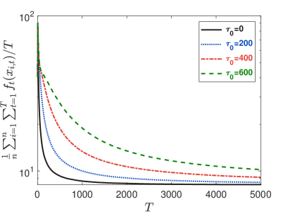
Figure 1: Evolutions of $\frac{1}{n}\sum\nolimits_{i=1}^{n}{\sum\nolimits_{t=1}^{T}{{f_{t}}({{x_{i,t}}})}}/T$.

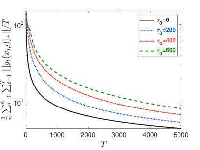
Figure 2: Evolutions of $\frac{1}{n}\sum\nolimits_{i=1}^{n}{\sum\nolimits_{t=1}^{T}{\|{{{[{{g_{t}}({{x_{i,t}}})}]}_{+}}}\|}}/T$.

Figure 3: Number of triggers.

Set ${\alpha_{t}}=1/{t^{1/2}}$, ${\beta_{t}}=1/{t^{1/2}}$, ${\gamma_{t}}=1/{t^{1/2}}$ and ${\tau_{t}}={\tau_{0}}/t$ for Algorithm 1. To explore the impact of different event-triggering threshold sequences on network regret and cumulative constraint violation, we select ${\tau_{0}}=0$, ${\tau_{0}}=200$, ${\tau_{0}}=400$, ${\tau_{0}}=600$ and ${\tau_{0}}=800$, respectively. With different values of ${\tau_{0}}$, Figs. 1–3 illustrate the evolutions of the average cumulative loss $\frac{1}{n}\sum\nolimits_{i=1}^{n}{\sum\nolimits_{t=1}^{T}{{f_{t}}({{x_{i,t}}})}}/T$, the average cumulative constraint violation $\frac{1}{n}\sum\nolimits_{i=1}^{n}{\sum\nolimits_{t=1}^{T}{\|{{{[{{g_{t}}({{x_{i,t}}})}]}_{+}}}\|}}/T$, and total number of triggers, respectively. Fig. 1 shows the larger ${\tau_{0}}$ is, the larger the average cumulative loss is. Fig. 2 shows the larger ${\tau_{0}}$ is, the larger the average cumulative constraint violation is. Fig. 3 shows the larger ${\tau_{0}}$ is, the less total number of triggers is. The results show the trade-off between the performance of Algorithm 1 and total number of communications, which conform to our theoretical results.

VI CONCLUSIONS

This paper considered the distributed online convex optimization problem with time-varying inequality constraints. We proposed the distributed event-triggered online primal–dual algorithm to reduce communication overhead via a time-varying directed graph. We analyzed the network regret and cumulative constraint violation of the proposed algorithm. Our results broaden the applicability of event-triggered online convex optimization to the regime with inequality constraints. Moreover, distributed settings, time-varying inequality constraints, cumulative constraint violation, time-varying directed graph and event-triggered communication were considered. The future directions are to consider the dynamic event-triggered communication such that total number of communications can be further reduced, and consider bandit feedback due to the unavailability of gradient information.

APPENDIX

VI-A Preliminary Lemmas

To prove Theorems 1 and 2, some preliminary results are derived in this section.

Lemma 1.

Suppose Assumption 2 hold. For all $i\in[n]$ and $t\in{\mathbb{N}_{+}}$, ${{\hat{x}}_{i,t}}$ generated by Algorithm 1 satisfy

$$\|{{{\hat{x}}_{i,t}}-{{\bar{x}}_{t}}}\| \leq\tau{\lambda^{t-2}}\sum\limits_{j=1}^{n}{\|{{{\hat{x}}_{j,1}}}\|}+\frac{1}{n}\sum\limits_{j=1}^{n}{\|{\hat{\varepsilon}_{j,t-1}^{x}}\|}+\|{\hat{\varepsilon}_{i,t-1}^{x}}\|$$

$$\;\;+\tau\sum\limits_{s=1}^{t-2}{{\lambda^{t-s-2}}}\sum\limits_{j=1}^{n}{\|{\hat{\varepsilon}_{j,s}^{x}}\|},$$ (48)

where ${{\bar{x}}_{t}}=\frac{1}{n}\sum\nolimits_{j=1}^{n}{{{\hat{x}}_{j,t}}}$ and $\hat{\varepsilon}_{i,t-1}^{x}={{\hat{x}}_{i,t}}-{z_{i,t}}$.

Proof. The proof is presented in Lemma 4 of [30].

Lemma 2.

Suppose Assumptions 1 and 2 hold, and ${\gamma_{t}}{\beta_{t}}\leq 1$, $t\in{\mathbb{N}_{+}}$. For all $i\in[n]$ and $t\in{\mathbb{N}_{+}}$, the sequences ${q_{i,t}}$ generated by Algorithm 1 satisfy

$${\Delta_{i,t}}({{\mu_{i}}}) \leq{\varpi_{1}}{\gamma_{t}}+q_{i,t-1}^{T}{b_{i,t}}-\mu_{i}^{T}{[{{g_{i,t-1}}({{x_{i,t-1}}})}]_{+}}$$

$$\;\;+\frac{1}{2}{\beta_{t}}{\|{{\mu_{i}}}\|^{2}}+{F_{2}}\|{{\mu_{i}}}\|\|{{x_{i,t}}-{x_{i,t-1}}}\|.$$ (49)

where ${\Delta_{i,t}}({{\mu_{i}}})=\frac{1}{{2{\gamma_{t}}}}\big{(}{{{\|{{q_{i,t}}-{\mu_{i}}}\|}^{2}}-({1-{\beta_{t}}{\gamma_{t}}}){{\|{{q_{i,t-1}}-{\mu_{i}}}\|}^{2}}}\big{)}$ with ${{\mu_{i}}}$ being an arbitrary vector in $\mathbb{R}_{+}^{{m_{i}}}$, ${\varpi_{1}}=2{({{F_{1}}+{F_{2}}R(\mathbb{X})})^{2}}$, and ${b_{i,t}}={[{{g_{i,t-1}}({{x_{i,t-1}}})}]_{+}}+{\big{(}{\partial{{[{{g_{i,t-1}}({{x_{i,t-1}}})}]}_{+}}}\big{)}^{T}}({{x_{i,t}}-{x_{i,t-1}}})$

Proof. The proof is presented in Lemma 5 of [30].

Lemma 3.

Suppose Assumptions 1–3 hold. For all $i\in[n]$, let $\{{{x_{i,t}}}\}$ be the sequences generated by Algorithm 1 and $\{{{y_{t}}}\}$ be an arbitrary sequence in $\mathbb{X}$, then

$$\;\;\;\;\;\frac{1}{n}\sum\limits_{i=1}^{n}{{f_{t}}({{x_{i,t}}})}-{f_{t}}({{y_{t}}})$$

$$\leq\frac{1}{n}\sum\limits_{i=1}^{n}{q_{i,t}^{T}\big{(}{{{[{{g_{i,t}}({{y_{t}}})}]}_{+}}-{b_{i,t+1}}}\big{)}-\frac{1}{{2n{\alpha_{t+1}}}}}\sum\limits_{i=1}^{n}{{{\|\varepsilon_{i,t}^{x}\|}^{2}}}$$

$$\;\;+\frac{1}{n}\sum\limits_{i=1}^{n}{{F_{2}}({2\|{{{\hat{x}}_{i,t}}-{{\bar{x}}_{t}}}\|+\|{{x_{i,t}}-{x_{i,t+1}}}\|})}+2{F_{2}}{\tau_{t}}$$

$$\;\;+\frac{1}{{2n{\alpha_{t+1}}}}\sum\limits_{i=1}^{n}({{\|{{y_{t}}-{z_{i,t+1}}}\|}^{2}}-{{\|{{y_{t+1}}-{z_{i,t+2}}}\|}^{2}}$$

$$\;\;+{{\|{{y_{t+1}}-{{\hat{x}}_{i,t+1}}}\|}^{2}}-{{\|{{y_{t}}-{x_{i,t+1}}}\|}^{2}}).$$ (50)

where $\varepsilon_{i,t}^{x}={x_{i,t+1}}-{z_{i,t+1}}$.

Proof. From Assumption 1, for $i\in[n]$, $t\in{\mathbb{N}_{+}}$, $x,y\in\mathbb{X}$, we have

$$|{{f_{i,t}}(x)-{f_{i,t}}(y)}| \leq{F_{2}}\|{x-y}\|,$$ (51a)

$$\|{{g_{i,t}}(x)-{g_{i,t}}(y)}\| \leq{F_{2}}\|{x-y}\|.$$ (51b)

From Algorithm 1, for any $t\in{\mathbb{N}_{+}}$, if $\|{{x_{i,t+1}}-{{\hat{x}}_{i,t}}}\|\geq{\tau_{t+1}}$, then $\|{{{\hat{x}}_{i,t+1}}-{x_{i,t+1}}}\|\leq{\tau_{t+1}}$. If $\|{{x_{i,t+1}}-{{\hat{x}}_{i,t}}}\|<{\tau_{t+1}}$, then ${{\hat{x}}_{i,t+1}}={{\hat{x}}_{i,t}}$ and we still have $\|{{{\hat{x}}_{i,t+1}}-{x_{i,t+1}}}\|\leq{\tau_{t+1}}$. Therefore, we always have $\|{{{\hat{x}}_{i,t}}-{x_{i,t}}}\|\leq{\tau_{t}}$ for any $t\geq 2$, $i\in[n]$. Recall that ${{\hat{x}}_{i,1}}={x_{i,1}}$. Thus, $\|{{{\hat{x}}_{i,t}}-{x_{i,t}}}\|\leq{\tau_{t}}$ for any $t\geq 1$, $i\in[n]$.

From (27a) and $\|{{{\hat{x}}_{i,t}}-{x_{i,t}}}\|\leq{\tau_{t}}$, we have

$$\;\;\;\;\;\frac{1}{n}\sum\limits_{i=1}^{n}{{f_{t}}({{x_{i,t}}})}$$

$$=\frac{1}{n}\sum\limits_{i=1}^{n}{{f_{i,t}}({{x_{i,t}}})}+\frac{1}{{{n^{2}}}}\sum\limits_{i=1}^{n}{\sum\limits_{j=1}^{n}{\big{(}{{f_{j,t}}({{x_{i,t}}})-{f_{j,t}}({{x_{j,t}}})}\big{)}}}$$

$$\leq\frac{1}{n}\sum\limits_{i=1}^{n}{{f_{i,t}}({{x_{i,t}}})}+\frac{{{F_{2}}}}{{{n^{2}}}}\sum\limits_{i=1}^{n}{\sum\limits_{j=1}^{n}{\|{{x_{i,t}}-{x_{j,t}}}\|}}$$

$$\leq\frac{1}{n}\sum\limits_{i=1}^{n}{{f_{i,t}}({{x_{i,t}}})}+\frac{{2{F_{2}}}}{n}\sum\limits_{i=1}^{n}{\|{{{\hat{x}}_{i,t}}-{{\bar{x}}_{t}}}\|}+2{F_{2}}{\tau_{t}}.$$ (52)

It then follows from the proof of Lemma 6 of [30] that (26) holds.

Lemma 4.

Suppose Assumptions 1–3 hold, and ${\gamma_{t}}{\beta_{t}}\leq 1$, $t\in{\mathbb{N}_{+}}$. For all $i\in[n]$, let $\{{{x_{i,t}}}\}$ be the sequences generated by Algorithm 1. Then, for any comparator sequence ${y_{[T]}}\in~{}{\mathcal{X}_{T}}$,

$$\;\;\;\;\;{{\rm{Net}\mbox{-}\rm{Reg}}({\{{{x_{i,t}}}\},{y_{[T]}}})}$$

$$\leq 4{F_{2}}{\varpi_{2}}+{\varpi_{1}}\sum\limits_{t=1}^{T}{{\gamma_{t}}}+10{\varpi_{6}}\sum\limits_{t=1}^{T}{\alpha_{t}}+{\varpi_{7}}\sum\limits_{t=1}^{T}{{\tau_{t}}}$$

$$\;\;+2R(\mathbb{X})\sum\limits_{t=1}^{T}{\frac{{{\tau_{t+1}}}}{{{\alpha_{t+1}}}}}+\frac{{2R{{(\mathbb{X})}^{2}}}}{{{\alpha_{T+1}}}}+\frac{{2R(\mathbb{X})}}{{{\alpha_{T}}}}{P_{T}}$$

$$\;\;-\frac{1}{{2n}}\sum\limits_{t=1}^{T}{\sum\limits_{i=1}^{n}{({\frac{1}{{{\gamma_{t}}}}-\frac{1}{{{\gamma_{t+1}}}}+{\beta_{t+1}}})}}{\|{{q_{i,t}}}\|^{2}},$$ (53)

$$\;\;\;\;\;\frac{1}{n}\sum\limits_{i=1}^{n}{{\|{\sum\limits_{t=1}^{T}{{{[{{g_{t}}({{x_{i,t}}})}]}_{+}}}}\|^{2}}}$$

$$\leq 8n{F_{1}}{F_{2}}{\varpi_{2}}T+2n{F_{1}}{\varpi_{10}}T\sum\limits_{t}^{T}{{\tau_{t}}}$$

$$\;\;+2\big{(}{\frac{1}{{{\gamma_{1}}}}+\sum\limits_{t=1}^{T}{({{\beta_{t}}+{\varpi_{9}}{\alpha_{t}}})}}\big{)}\big{(}n{F_{1}}T+4n{F_{2}}{\varpi_{2}}$$

$$\;\;+n{\varpi_{1}}\sum\limits_{t=1}^{T}{{\gamma_{t}}}+20n{\varpi_{6}}\sum\limits_{t=1}^{T}{{\alpha_{t}}}+2n{\varpi_{11}}\sum\limits_{t=1}^{T}{{\tau_{t}}}$$

$$\;\;+2nR(\mathbb{X})\sum\limits_{t=1}^{T}{\frac{{{\tau_{t+1}}}}{{{\alpha_{t+1}}}}}+\frac{{2nR{{(\mathbb{X})}^{2}}}}{{{\alpha_{T+1}}}}$$

$$\;\;-\frac{1}{2}\sum\limits_{t=1}^{T}{\sum\limits_{i=1}^{n}{({\frac{1}{{{\gamma_{t}}}}-\frac{1}{{{\gamma_{t+1}}}}+{\beta_{t+1}}}){\|{{q_{i,t}}-\mu_{ij}^{0}}\|^{2}}}}\big{)}.$$ (54)

where ${\varpi_{2}}=\frac{\tau}{{\lambda({1-\lambda})}}\sum\limits_{i=1}^{n}{\|{{{\hat{x}}_{i,1}}}\|}$, ${\varpi_{3}}=2{F_{2}}+\frac{{{n^{2}}{\tau^{2}}{F_{2}}}}{{2{{\left({1-\lambda}\right)}^{2}}}}$, ${\varpi_{4}}=2+\frac{{n\tau}}{{1-\lambda}}$, ${\varpi_{5}}=2{F_{2}}{\varpi_{2}}+\frac{{F_{2}^{2}}}{4}$, ${\varpi_{6}}=2{F_{2}}{\varpi_{3}}+{\varpi_{5}}$, ${\varpi_{7}}=4{F_{2}}{\varpi_{4}}+2{F_{2}}$, ${\varpi_{8}}=1+{\varpi_{4}}$, ${\varpi_{9}}=20{\varpi_{6}}$, ${\varpi_{10}}=3{F_{2}}{\varpi_{4}}+{F_{2}}{\varpi_{8}}$, ${\varpi_{11}}=2{F_{2}}{\varpi_{4}}+{F_{2}}$, and $\mu_{ij}^{0}=\frac{{\sum\nolimits_{t=1}^{T}{{{[{{g_{i,t}}({{x_{j,t}}})}]}_{+}}}}}{{\frac{1}{{{\gamma_{1}}}}+\sum\nolimits_{t=1}^{T}{({{\beta_{t}}+{\varpi_{9}}{\alpha_{t}}})}}}$.

Proof. ($\mathbf{i}$) We first provide a loose bound for network regret.

From (5), we have

$$\;\;\;\;\;{\|{{y_{t+1}}-{{\hat{x}}_{i,t+1}}}\|^{2}}-{\|{{y_{t}}-{x_{i,t+1}}}\|^{2}}$$

$$\leq\|{{y_{t+1}}-{y_{t}}-{{\hat{x}}_{i,t+1}}+{x_{i,t+1}}}\|\|{{y_{t+1}}-{x_{i,t+1}}+{y_{t}}-{x_{i,t+1}}}\|$$

$$\leq 4R(\mathbb{X})\|{{y_{t+1}}-{y_{t}}}\|+4R(\mathbb{X}){\tau_{t+1}}.$$ (55)

From (25), (26) and (31), we have

$$\;\;\;\;\;\frac{1}{n}\sum\limits_{i=1}^{n}{\big{(}{{\Delta_{i,t+1}}({{\mu_{i}}})+\mu_{i}^{T}{{[{{g_{i,t}}({{x_{i,t}}})}]}_{+}}-\frac{1}{2}{\beta_{t+1}}{{\|{{\mu_{i}}}\|}^{2}}}\big{)}}$$

$$\;\;+\frac{1}{n}\sum\limits_{i=1}^{n}{{f_{t}}({{x_{i,t}}})}-{f_{t}}({{y_{t}}})$$

$$\leq{\varpi_{1}}{\gamma_{t+1}}+\frac{1}{n}\sum\limits_{i=1}^{n}{{{\tilde{\Delta}}_{i,t+1}}({{\mu_{i}}})}$$

$$\;\;+\frac{1}{{2n{\alpha_{t+1}}}}\sum\limits_{i=1}^{n}{({{{\|{{y_{t}}-{z_{i,t+1}}}\|}^{2}}-{{\|{{y_{t+1}}-{z_{i,t+2}}}\|}^{2}}})}$$

$$\;\;+2{F_{2}}{\tau_{t}}+\frac{{2R(\mathbb{X}){\tau_{t+1}}}}{{{\alpha_{t+1}}}}+\frac{{2R(\mathbb{X})}}{{{\alpha_{t+1}}}}\|{{y_{t+1}}-{y_{t}}}\|,$$ (56)

where

$${{\tilde{\Delta}}_{i,t+1}}({{\mu_{i}}}) ={F_{2}}({\|{{\mu_{i}}}\|+1})\|{{x_{i,t}}-{x_{i,t+1}}}\|$$

$$\;\;+2{F_{2}}\|{{{\hat{x}}_{i,t}}-{{\bar{x}}_{t}}}\|-\frac{1}{{2{\alpha_{t+1}}}}{\|{\varepsilon_{i,t}^{x}}\|^{2}}.$$

From (5) and $\{{{\alpha_{t}}}\}$ is non-increasing, we have

$$\;\;\;\;\;\sum\limits_{t=1}^{T}{\frac{1}{{{\alpha_{t+1}}}}}({{{\|{{y_{t}}-{z_{i,t+1}}}\|}^{2}}-{{\|{{y_{t+1}}-{z_{i,t+2}}}\|}^{2}}})$$

$$=\sum\limits_{t=1}^{T}\big{(}{\frac{1}{{{\alpha_{t}}}}{{\|{{y_{t}}-{z_{i,t+1}}}\|}^{2}}-\frac{1}{{{\alpha_{t+1}}}}{{\|{{y_{t+1}}-{z_{i,t+2}}}\|}^{2}}}$$

$$\;\;+({\frac{1}{{{\alpha_{t+1}}}}-\frac{1}{{{\alpha_{t}}}}}){{\|{{y_{t}}-{z_{i,t+1}}}\|}^{2}}\big{)}$$

$$\leq\frac{1}{{{\alpha_{1}}}}{\|{{y_{1}}-{z_{i,2}}}\|^{2}}-\frac{1}{{{\alpha_{T+1}}}}{\|{{y_{T+1}}-{z_{i,T+2}}}\|^{2}}$$

$$\;\;+\sum\limits_{t=1}^{T}{({\frac{1}{{{\alpha_{t+1}}}}-\frac{1}{{{\alpha_{t}}}}})4R{(\mathbb{X})^{2}}}\leq\frac{{4R{(\mathbb{X})^{2}}}}{{{\alpha_{T+1}}}}.$$ (57)

From (33) and $\{{{\alpha_{t}}}\}$ is non-increasing, setting ${y_{T+1}}={y_{T}}$ and ${\mu_{i}}={0_{{m_{i}}}}$, summing (32) over $t\in\left[T\right]$ gives

$$\;\;\;\;\;{{\rm{Net}\mbox{-}\rm{Reg}}({\{{{x_{i,t}}}\},{y_{[T]}}})}+\frac{1}{n}\sum\limits_{t=1}^{T}{\sum\limits_{i=1}^{n}{{\Delta_{i,t+1}}({{\mathbf{0}_{{m_{i}}}}})}}$$

$$\leq{\varpi_{1}}\sum\limits_{t=1}^{T}{{\gamma_{t+1}}}+\frac{1}{n}\sum\limits_{t=1}^{T}{\sum\limits_{i=1}^{n}{{{\tilde{\Delta}}_{i,t+1}}({{\mathbf{0}_{{m_{i}}}}})}}+\sum\limits_{t=1}^{T}{2{F_{2}}{\tau_{t}}}$$

$$\;\;+\sum\limits_{t=1}^{T}{\frac{{2R(\mathbb{X}){\tau_{t+1}}}}{{{\alpha_{t+1}}}}}+\frac{{2R{{(\mathbb{X})}^{2}}}}{{{\alpha_{T+1}}}}+\frac{{2R(\mathbb{X})}}{{{\alpha_{T}}}}{P_{T}}.$$ (58)

We then establish a lower bound for network regret.

For any $T\in{\mathbb{N}_{+}}$, we have

$$\sum\limits_{t=1}^{T}{{\Delta_{i,t+1}}({{\mu_{i}}})} =\frac{1}{2}\sum\limits_{t=1}^{T}{({\frac{1}{{{\gamma_{t}}}}-\frac{1}{{{\gamma_{t+1}}}}+{\beta_{t+1}}}){{\|{{q_{i,t}}-{\mu_{i}}}\|}^{2}}}$$

$$\;\;+\frac{{{{\|{{q_{i,T+1}}-{\mu_{i}}}\|}^{2}}}}{{2{\gamma_{T+1}}}}-\frac{{{{\|{{\mu_{i}}}\|}^{2}}}}{{2{\gamma_{1}}}}.$$ (59)

Substituting ${\mu_{i}}={\mathbf{0}_{{m_{i}}}}$ into (35) yields

$$\sum\limits_{t=1}^{T}{{\Delta_{i,t+1}}({{\mathbf{0}_{{m_{i}}}}})}\geq\frac{1}{2}\sum\limits_{t=1}^{T}{({\frac{1}{{{\gamma_{t}}}}-\frac{1}{{{\gamma_{t+1}}}}+{\beta_{t+1}}}){{\|{{q_{i,t}}}\|}^{2}}}.$$ (60)

We have

$$\sum\limits_{t=1}^{T}{\sum\limits_{s=1}^{t-2}{{\lambda^{t-s-2}}\sum\limits_{j=1}^{n}{\|{\hat{\varepsilon}_{j,s}^{x}}\|}}} =\sum\limits_{t=1}^{T-2}{\sum\limits_{j=1}^{n}{\|{\hat{\varepsilon}_{j,t}^{x}}\|\sum\limits_{s=0}^{T-t-2}{{\lambda^{s}}}}}$$

$$\leq\frac{1}{{1-\lambda}}\sum\limits_{t=1}^{T-2}{\sum\limits_{j=1}^{n}{\|{\hat{\varepsilon}_{j,t}^{x}}\|}}.$$ (61)

and

$$\|{\hat{\varepsilon}_{i,t-1}^{x}}\| =\|{{{\hat{x}}_{i,t}}-{x_{i,t}}+{x_{i,t}}-{z_{i,t}}}\|$$

$$\leq\|{\varepsilon_{i,t-1}^{x}}\|+{\tau_{t}}.$$ (62)

From (24), (37) and (38), we have

$$\;\;\;\;\;\sum\limits_{t=1}^{T}{\|{{{\hat{x}}_{i,t}}-{{\bar{x}}_{t}}}\|}$$

$$\leq{\varpi_{2}}+\frac{1}{n}\sum\limits_{t=1}^{T}{\sum\limits_{j=1}^{n}{\|{\varepsilon_{j,t-1}^{x}}\|}}+\sum\limits_{t=1}^{T}{\|{\varepsilon_{i,t-1}^{x}}\|}$$

$$+\frac{\tau}{{1-\lambda}}\sum\limits_{t=1}^{T-2}{\sum\limits_{j=1}^{n}{\|{\varepsilon_{j,t}^{x}}\|}}+2\sum\limits_{t=1}^{T}{{\tau_{t}}}+\frac{{n\tau}}{{1-\lambda}}\sum\limits_{t=1}^{T-2}{{\tau_{t+1}}}.$$ (63)

For any ${\mu_{i}}\in{\mathbb{R}^{{m_{i}}}}$ and $a>0$, it follows from (39) that

$$\;\;\;\;\;\sum\limits_{t=1}^{T}{\sum\limits_{i=1}^{n}{\|{{\mu_{i}}}\|\|{{{\hat{x}}_{i,t}}-{{\bar{x}}_{t}}}\|}}$$

$$\leq{\varpi_{2}}\sum\limits_{i=1}^{n}{\|{{\mu_{i}}}\|}$$

$$+\frac{1}{n}\sum\limits_{t=2}^{T}{\sum\limits_{i=1}^{n}{\sum\limits_{j=1}^{n}{({\frac{1}{{4a{F_{2}}{\alpha_{t}}}}{{\|{\varepsilon_{i,t-1}^{x}}\|}^{2}}+a{F_{2}}{\alpha_{t}}{{\|{{\mu_{j}}}\|}^{2}}})}}}$$

$$+\sum\limits_{t=2}^{T}{\sum\limits_{i=1}^{n}{({\frac{1}{{4a{F_{2}}{\alpha_{t}}}}{{\|{\varepsilon_{i,t-1}^{x}}\|}^{2}}+a{F_{2}}{\alpha_{t}}{{\|{{\mu_{i}}}\|}^{2}}})}}$$

$$+\sum\limits_{t=2}^{T}{\sum\limits_{i=1}^{n}{\sum\limits_{j=1}^{n}{({\frac{1}{{2an{F_{2}}{\alpha_{t}}}}{{\|{\varepsilon_{i,t-1}^{x}}\|}^{2}}+\frac{{an{F_{2}}{\tau^{2}}{\alpha_{t}}}}{{2{{({1-\lambda})}^{2}}}}{{\|{{\mu_{j}}}\|}^{2}}})}}}$$

$$+\sum\limits_{t=1}^{T}{\sum\limits_{i=1}^{n}{2{\tau_{t}}\|{{\mu_{i}}}\|}}+\frac{{n\tau}}{{1-\lambda}}\sum\limits_{t=2}^{T}{\sum\limits_{i=1}^{n}{{\tau_{t}}\|{{\mu_{i}}}\|}}$$

$$\leq{\varpi_{2}}\sum\limits_{i=1}^{n}{\|{{\mu_{i}}}\|}+\sum\limits_{t=2}^{T}{\sum\limits_{i=1}^{n}{\frac{1}{{a{F_{2}}{\alpha_{t}}}}{{\|{\varepsilon_{i,t-1}^{x}}\|}^{2}}}}$$

$$+\sum\limits_{t=2}^{T}{\sum\limits_{i=1}^{n}{a{\varpi_{3}}{\alpha_{t}}{{\|{{\mu_{i}}}\|}^{2}}}}+{\varpi_{4}}\sum\limits_{t=1}^{T}{\sum\limits_{i=1}^{n}{{\tau_{t}}\|{{\mu_{i}}}\|}}.$$ (64)

For any ${\mu_{i}}\in{\mathbb{R}^{{m_{i}}}}$ and $a>0$, we have

$$\;\;\;\;\;\|{{\mu_{i}}}\|\|{{x_{i,t}}-{x_{i,t+1}}}\|$$

$$\leq\|{{\mu_{i}}}\|\|{{x_{i,t}}-{z_{i,t+1}}}\|+\|{{\mu_{i}}}\|\|{{z_{i,t+1}}-{x_{i,t+1}}}\|$$

$$\leq\|{{\mu_{i}}}\|\|{{x_{i,t}}-{z_{i,t+1}}}\|$$

$$\;\;+\frac{1}{{a{F_{2}}{\alpha_{t+1}}}}{\|{\varepsilon_{i,t}^{x}}\|^{2}}+\frac{{a{F_{2}}{\alpha_{t+1}}}}{4}{\|{{\mu_{i}}}\|^{2}}.$$ (65)

From (8) and ${\sum\nolimits_{i=1}^{n}{[{{W_{t}}}]}_{ij}}={\sum\nolimits_{j=1}^{n}{[{{W_{t}}}]}_{ij}}=1$, we have

$$\;\;\;\;\;\sum\limits_{i=1}^{n}{\|{{x_{i,t}}-{z_{i,t+1}}}\|}$$

$$\leq\sum\limits_{i=1}^{n}{({\|{{x_{i,t}}-{{\bar{x}}_{t}}}\|+\|{{{\bar{x}}_{t}}-{z_{i,t+1}}}\|})}$$

$$\leq\sum\limits_{i=1}^{n}{({\|{{x_{i,t}}-{{\hat{x}}_{i,t}}+{{\hat{x}}_{i,t}}-{{\bar{x}}_{t}}}\|+\|{{{\bar{x}}_{t}}-\sum\limits_{j=1}^{n}{{{[{{W_{t}}}]}_{ij}}{{\hat{x}}_{j,t}}}}\|})}$$

$$\leq\sum\limits_{i=1}^{n}{({\|{{{\hat{x}}_{i,t}}-{x_{i,t}}}\|+\|{{{\hat{x}}_{i,t}}-{{\bar{x}}_{t}}}\|})}$$

$$\;\;+\sum\limits_{i=1}^{n}{\sum\limits_{j=1}^{n}{{{[{{W_{t}}}]}_{ij}}\|{{{\bar{x}}_{t}}-\sum\limits_{j=1}^{n}{{{[{{W_{t}}}]}_{ij}}{{\hat{x}}_{j,t}}}}\|}}$$

$$\leq 2\sum\limits_{i=1}^{n}{\|{{{\hat{x}}_{i,t}}-{{\bar{x}}_{t}}}\|}+n{\tau_{t}}.$$ (66)

From (40)–(42), for any ${\mu_{i}}\in{\mathbb{R}^{{m_{i}}}}$ and $a>0$, we have

$$\;\;\;\;\;\sum\limits_{t=1}^{T}{\sum\limits_{i=1}^{n}{{F_{2}}\|{{\mu_{i}}}\|\|{{x_{i,t}}-{x_{i,t+1}}}\|}}$$

$$\leq\sum\limits_{t=1}^{T}{\sum\limits_{i=1}^{n}{2{F_{2}}\|{{\mu_{i}}}\|\|{{x_{i,t}}-{{\bar{x}}_{t}}}\|}}$$

$$+\sum\limits_{t=1}^{T}{\sum\limits_{i=1}^{n}{\frac{1}{{a{\alpha_{t+1}}}}{{\|{\varepsilon_{i,t}^{x}}\|}^{2}}}}+\sum\limits_{t=1}^{T}{\sum\limits_{i=1}^{n}{\frac{{aF_{2}^{2}{\alpha_{t+1}}}}{4}{{\|{{\mu_{i}}}\|}^{2}}}}$$

$$\leq 2{F_{2}}{\varpi_{2}}\sum\limits_{i=1}^{n}{\|{{\mu_{i}}}\|}+\sum\limits_{t=2}^{T}{\sum\limits_{i=1}^{n}{\frac{2}{{a{\alpha_{t}}}}{{\|{\varepsilon_{i,t-1}^{x}}\|}^{2}}}}$$

$$\;\;+\sum\limits_{t=2}^{T}{\sum\limits_{i=1}^{n}{4aF_{2}^{2}{\alpha_{t}}{{\|{{\mu_{i}}}\|}^{2}}}}+\sum\limits_{t=2}^{T}{\sum\limits_{i=1}^{n}{\frac{{a{n^{2}}{\tau^{2}}F_{2}^{2}{\alpha_{t}}}}{{{{({1-\lambda})}^{2}}}}{{\|{{\mu_{i}}}\|}^{2}}}}$$

$$\;\;+4{F_{2}}\sum\limits_{t=1}^{T}{\sum\limits_{i=1}^{n}{{\tau_{t}}\|{{\mu_{i}}}\|}}+\frac{{2n\tau{F_{2}}}}{{1-\lambda}}\sum\limits_{t=2}^{T}{\sum\limits_{i=1}^{n}{{\tau_{t}}\|{{\mu_{i}}}\|}}$$

$$\;\;+\sum\limits_{t=1}^{T}{\sum\limits_{i=1}^{n}{\frac{1}{{a{\alpha_{t+1}}}}{{\|{\varepsilon_{i,t}^{x}}\|}^{2}}}}+\sum\limits_{t=1}^{T}{\sum\limits_{i=1}^{n}{\frac{{aF_{2}^{2}{\alpha_{t+1}}}}{4}{{\|{{\mu_{i}}}\|}^{2}}}}$$

$$\leq 2{F_{2}}{\varpi_{2}}\sum\limits_{i=1}^{n}{\|{{\mu_{i}}}\|}+\sum\limits_{t=1}^{T}{\sum\limits_{i=1}^{n}{a{\varpi_{5}}{\alpha_{t}}{{\|{{\mu_{i}}}\|}^{2}}}}$$

$$\;\;+\sum\limits_{t=1}^{T}{\sum\limits_{i=1}^{n}{\frac{3}{{a{\alpha_{t+1}}}}{{\|{\varepsilon_{i,t}^{x}}\|}^{2}}}}+2{F_{2}}{\varpi_{4}}\sum\limits_{t=1}^{T}{\sum\limits_{i=1}^{n}{{\tau_{t}}\|{{\mu_{i}}}\|}}.$$ (67)

Choosing $\|{{\mu_{i}}}\|=1$ in (40) and (43) yields

$$\;\;\;\;\;\sum\limits_{t=1}^{T}{\sum\limits_{i=1}^{n}{2{F_{2}}\|{{{\hat{x}}_{i,t}}-{{\bar{x}}_{t}}}\|}}$$

$$\leq 2n{F_{2}}{\varpi_{2}}+2n{F_{2}}{\varpi_{4}}\sum\limits_{t=1}^{T}{{\tau_{t}}}$$

$$\;\;+\sum\limits_{t=2}^{T}{\sum\limits_{i=1}^{n}{({2a{F_{2}}{\varpi_{3}}{\alpha_{t}}+\frac{2}{{a{\alpha_{t}}}}{{\|{\varepsilon_{i,t-1}^{x}}\|}^{2}}})}},$$ (68)

and

$$\;\;\;\;\;\sum\limits_{t=1}^{T}{\sum\limits_{i=1}^{n}{{F_{2}}\left\|{{x_{i,t}}-{x_{i,t+1}}}\right\|}}$$

$$\leq 2n{F_{2}}{\varpi_{2}}+\sum\limits_{t=1}^{T}{an{\varpi_{5}}{\alpha_{t+1}}}$$

$$\;\;+\sum\limits_{t=1}^{T}{\sum\limits_{i=1}^{n}{\frac{3}{{a{\alpha_{t+1}}}}{{\left\|{\varepsilon_{i,t}^{x}}\right\|}^{2}}}}+2n{F_{2}}{\varpi_{4}}\sum\limits_{t=1}^{T}{{\tau_{t}}}.$$ (69)

From (43)–(45), and choosing $a=10$ yields

$$\;\;\;\;\;\sum\limits_{t=1}^{T}{\sum\limits_{i=1}^{n}{{{\tilde{\Delta}}_{i,t+1}}({{\mathbf{0}_{{m_{i}}}}})}}\;\;\;\;\;\;\;\;\;\;\;\;\;\;\;\;\;\;\;\;\;\;\;\;\;\;\;\;\;\;\;\;\;\;\;\;\;\;\;\;\;\;\;\;\;\;\;\;\;\;\;\;$$

$$\leq 4n{F_{2}}{\varpi_{2}}+4n{F_{2}}{\varpi_{4}}\sum\limits_{t=1}^{T}{{\tau_{t}}}+\sum\limits_{t=2}^{T}{20n{F_{2}}{\varpi_{3}}{\alpha_{t}}}$$

$$\;\;+\sum\limits_{t=1}^{T}{10n{\varpi_{5}}{\alpha_{t+1}}}+\sum\limits_{t=1}^{T}{\sum\limits_{i=1}^{n}{\frac{3}{{10{\alpha_{t+1}}}}}}{\|{\varepsilon_{i,t}^{x}}\|^{2}}$$

$$\;\;+\sum\limits_{t=2}^{T}{\sum\limits_{i=1}^{n}{\frac{2}{{10{\alpha_{t}}}}}}{\|{\varepsilon_{i,t-1}^{x}}\|^{2}}-\sum\limits_{t=1}^{T}{\sum\limits_{i=1}^{n}{\frac{1}{{2{\alpha_{t+1}}}}}}{\|{\varepsilon_{i,t}^{x}}\|^{2}}$$

$$\leq 4n{F_{2}}{\varpi_{2}}+4n{F_{2}}{\varpi_{4}}\sum\limits_{t=1}^{T}{{\tau_{t}}}+\sum\limits_{t=1}^{T}{10n{\varpi_{6}}{\alpha_{t}}}.$$ (70)

Combining (34), (36) and (46) yields (29).

($\mathbf{ii}$) We first provide a loose bound for network cumulative constraint violation.

We have

$$\;\;\;\;\;\mu_{i}^{T}{[{{g_{i,t}}({{x_{i,t}}})}]_{+}}$$

$$=\mu_{i}^{T}{[{{g_{i,t}}({{x_{j,t}}})}]_{+}}+\mu_{i}^{T}{[{{g_{i,t}}({{x_{i,t}}})}]_{+}}-\mu_{i}^{T}{[{{g_{i,t}}({{x_{j,t}}})}]_{+}}$$

$$\geq\mu_{i}^{T}{[{{g_{i,t}}({{x_{j,t}}})}]_{+}}-\|{{\mu_{i}}}\|\|{{{[{{g_{i,t}}({{x_{i,t}}})}]}_{+}}-{{[{{g_{i,t}}({{x_{j,t}}})}]}_{+}}}\|$$

$$\geq\mu_{i}^{T}{[{{g_{i,t}}({{x_{j,t}}})}]_{+}}-\|{{\mu_{i}}}\|\|{{g_{i,t}}({{x_{i,t}}})-{g_{i,t}}({{x_{j,t}}})}\|$$

$$\geq\mu_{i}^{T}{[{{g_{i,t}}({{x_{j,t}}})}]_{+}}-{F_{2}}\|{{\mu_{i}}}\|\|{{x_{i,t}}-{x_{j,t}}}\|$$

$$\geq\mu_{i}^{T}{[{{g_{i,t}}({{x_{j,t}}})}]_{+}}$$

$$\;\;-{F_{2}}\|{{\mu_{i}}}\|\|{{{\hat{x}}_{i,t}}-{x_{i,t}}}\|-{F_{2}}\|{{\mu_{i}}}\|\|{{{\hat{x}}_{i,t}}-{{\bar{x}}_{t}}}\|$$

$$\;\;-{F_{2}}\|{{\mu_{i}}}\|\|{{{\hat{x}}_{j,t}}-{x_{j,t}}}\|-{F_{2}}\|{{\mu_{i}}}\|\|{{{\hat{x}}_{j,t}}-{{\bar{x}}_{t}}}\|,$$ (71)

where the second inequality holds since projection operator is non-expansive, and the third inequality holds due to (27b).

Combining (32) and (47), setting ${y_{t}}=y$, and summing over $j\in[n]$ yields

$$\;\;\;\;\;\sum\limits_{i=1}^{n}{\big{(}{{\Delta_{i,t+1}}({{\mu_{i}}})+\frac{1}{n}\sum\limits_{j=1}^{n}{\mu_{i}^{T}{{[{{g_{i,t}}({{x_{j,t}}})}]}_{+}}}-\frac{1}{2}{\beta_{t+1}}{{\|{{\mu_{i}}}\|}^{2}}}\big{)}}$$

$$\;\;+\sum\limits_{i=1}^{n}{{f_{t}}({{x_{i,t}}})}-n{f_{t}}(y)$$

$$\leq n{\varpi_{1}}{\gamma_{t+1}}+\sum\limits_{i=1}^{n}{{{\hat{\Delta}}_{i,t+1}}({{\mu_{i}}})}+\frac{1}{n}{\check{\Delta}_{t}}+2n{F_{2}}{\tau_{t}}+\frac{{2nR(\mathbb{X}){\tau_{t+1}}}}{{{\alpha_{t+1}}}}$$

$$\;\;+\frac{1}{{2{\alpha_{t+1}}}}\sum\limits_{i=1}^{n}{({{{\|{y-{z_{i,t+1}}}\|}^{2}}-\|{y-{z_{i,t+2}}}\|})},$$ (72)

where

$${{\hat{\Delta}}_{i,t+1}}({{\mu_{i}}}) ={{\tilde{\Delta}}_{i,t+1}}({{\mu_{i}}})+{F_{2}}\|{{\mu_{i}}}\|\|{{{\hat{x}}_{i,t}}-{{\bar{x}}_{t}}}\|+{F_{2}}\|{{\mu_{i}}}\|{\tau_{t}},$$

$${\check{\Delta}_{t}} =\sum\limits_{i=1}^{n}{\sum\limits_{j=1}^{n}{{F_{2}}\|{{\mu_{i}}}\|\|{{{\hat{x}}_{j,t}}-{{\bar{x}}_{t}}}\|}}+\sum\limits_{i=1}^{n}{n{F_{2}}\|{{\mu_{i}}}\|{\tau_{t}}}.$$

Combining (40), (43)–(45), and choosing $a=20$ yields

$$\;\;\;\;\;\sum\limits_{t=1}^{T}{\sum\limits_{i=1}^{n}{{{\hat{\Delta}}_{i,t+1}}({{\mu_{i}}})}}$$

$$\leq 4n{F_{2}}{\varpi_{2}}+20n{\varpi_{6}}\sum\limits_{t=1}^{T}{{\alpha_{t}}}+4n{F_{2}}{\varpi_{4}}\sum\limits_{t=1}^{T}{{\tau_{t}}}$$

$$\;\;+3{F_{2}}{\varpi_{2}}\sum\limits_{i=1}^{n}{\|{{\mu_{i}}}\|}+20({{F_{2}}{\varpi_{3}}+{\varpi_{5}}})\sum\limits_{t=1}^{T}{\sum\limits_{i=1}^{n}{{\alpha_{t}}{{\|{{\mu_{i}}}\|}^{2}}}}$$

$$\;\;+3{F_{2}}{\varpi_{4}}\sum\limits_{t=1}^{T}{\sum\limits_{i=1}^{n}{{\tau_{t}}\|{{\mu_{i}}}\|}}-\sum\limits_{t=1}^{T}{\sum\limits_{i=1}^{n}{\frac{1}{{20{\alpha_{t+1}}}}}}{\|{\varepsilon_{i,t}^{x}}\|^{2}}.$$ (73)

From (39), we have

$$\;\;\;\;\;\sum\limits_{t=1}^{T}{\sum\limits_{i=1}^{n}{\sum\limits_{j=1}^{n}{\|{{\mu_{j}}}\|\|{{{\hat{x}}_{i,t}}-{{\bar{x}}_{t}}}\|}}}$$

$$\leq n{\varpi_{2}}\sum\limits_{j=1}^{n}{\|{{\mu_{j}}}\|}+2\sum\limits_{t=2}^{T}{\sum\limits_{i=1}^{n}{\sum\limits_{j=1}^{n}{\|{\varepsilon_{i,t-1}^{x}}\|\|{{\mu_{j}}}\|}}}$$

$$\;\;+\frac{{n\tau}}{{1-\lambda}}\sum\limits_{t=2}^{T}{\sum\limits_{i=1}^{n}{\sum\limits_{j=1}^{n}{\|{\varepsilon_{i,t-1}^{x}}\|\|{{\mu_{j}}}\|}}}+n{\varpi_{4}}\sum\limits_{t=1}^{T}{\sum\limits_{j=1}^{n}{{\tau_{t}}\|{{\mu_{j}}}\|}}$$

$$\leq n{\varpi_{2}}\sum\limits_{j=1}^{n}{\|{{\mu_{j}}}\|}$$

$$\;\;+\sum\limits_{t=2}^{T}{\sum\limits_{i=1}^{n}{\sum\limits_{j=1}^{n}{({\frac{1}{{2a{F_{2}}{\alpha_{t}}}}{{\|{\varepsilon_{i,t-1}^{x}}\|}^{2}}+2a{F_{2}}{\alpha_{t}}{{\|{{\mu_{j}}}\|}^{2}}})}}}$$

$$\;\;+\sum\limits_{t=2}^{T}{\sum\limits_{i=1}^{n}{\sum\limits_{j=1}^{n}{({\frac{1}{{2a{F_{2}}{\alpha_{t}}}}{{\|{\varepsilon_{i,t-1}^{x}}\|}^{2}}+\frac{{a{n^{2}}{F_{2}}{\tau^{2}}{\alpha_{t}}}}{{2{{({1-\lambda})}^{2}}}}{{\|{{\mu_{j}}}\|}^{2}}})}}}$$

$$\;\;+n{\varpi_{4}}\sum\limits_{t=1}^{T}{\sum\limits_{j=1}^{n}{{\tau_{t}}\|{{\mu_{j}}}\|}}$$

$$=n{\varpi_{2}}\sum\limits_{i=1}^{n}{\|{{\mu_{i}}}\|}+\sum\limits_{t=2}^{T}{\sum\limits_{i=1}^{n}{an{\varpi_{3}}{\alpha_{t}}{{\|{{\mu_{i}}}\|}^{2}}}}$$

$$\;\;+\sum\limits_{t=2}^{T}{\sum\limits_{i=1}^{n}{\frac{n}{{a{F_{2}}{\alpha_{t}}}}}}{\|{\varepsilon_{i,t-1}^{x}}\|^{2}}+n{\varpi_{4}}\sum\limits_{t=1}^{T}{\sum\limits_{i=1}^{n}{{\tau_{t}}\|{{\mu_{i}}}\|}}.$$ (74)

Choosing $a=20$ in (50) yields

$$\;\;\;\;\;\frac{1}{n}\sum\limits_{t=1}^{T}{{\check{\Delta}_{t}}}$$

$$\leq{F_{2}}{\varpi_{2}}\sum\limits_{i=1}^{n}{\|{{\mu_{i}}}\|}+\sum\limits_{t=1}^{T}{\sum\limits_{i=1}^{n}{20{F_{2}}{\varpi_{3}}{\alpha_{t}}{{\|{{\mu_{i}}}\|}^{2}}}}$$

$$\;\;+\sum\limits_{t=2}^{T}{\sum\limits_{i=1}^{n}{\frac{1}{{20{\alpha_{t}}}}{{\|{\varepsilon_{i,t-1}^{x}}\|}^{2}}}}+{F_{2}}{\varpi_{8}}\sum\limits_{t=1}^{T}{\sum\limits_{i=1}^{n}{{\tau_{t}}\|{{\mu_{i}}}\|}}.$$ (75)

Let ${h_{ij}}:\mathbb{R}_{+}^{{m_{i}}}\to\mathbb{R}$ be a function defined as

$${h_{ij}}({{\mu_{i}}}) =\mu_{i}^{T}\sum\limits_{t=1}^{T}{{{[{{g_{i,t}}({{x_{j,t}}})}]}_{+}}}$$

$$\;\;-\frac{1}{2}{\|{{\mu_{i}}}\|^{2}}\big{(}{\frac{1}{{{\gamma_{1}}}}+\sum\limits_{t=1}^{T}{({{\beta_{t}}+{\varpi_{9}}{\alpha_{t}}})}}\big{)}.$$ (76)

From (33), (35), (49), (51), and (52), summing (48) over $t\in[T]$ gives

$$\;\;\;\;\;\frac{1}{2}\sum\limits_{t=1}^{T}{\sum\limits_{i=1}^{n}{({\frac{1}{{{\gamma_{t}}}}-\frac{1}{{{\gamma_{t+1}}}}+{\beta_{t+1}}}){{\|{{q_{i,t}}-{\mu_{i}}}\|}^{2}}}}\;\;\;\;\;\;\;\;\;\;$$

$$\;\;+\frac{1}{n}\sum\limits_{i=1}^{n}{\sum\limits_{j=1}^{n}{{h_{ij}}({{\mu_{i}}})}}+n{{\rm{Net}\mbox{-}\rm{Reg}}({\{{{x_{i,t}}}\},{y}})}$$

$$\leq 4n{F_{2}}{\varpi_{2}}+n{\varpi_{1}}\sum\limits_{t=1}^{T}{{\gamma_{t}}}+20n{\varpi_{6}}\sum\limits_{t=1}^{T}{{\alpha_{t}}}+2n{\varpi_{11}}\sum\limits_{t=1}^{T}{{\tau_{t}}}$$

$$\;\;+4{F_{2}}{\varpi_{2}}\sum\limits_{i=1}^{n}{\|{{\mu_{i}}}\|}+{\varpi_{10}}\sum\limits_{t=1}^{T}{\sum\limits_{i=1}^{n}{{\tau_{t}}\|{{\mu_{i}}}\|}}\;\;\;\;\;\;\;\;\;\;\;\;\;\;$$

$$\;\;+2nR(\mathbb{X})\sum\limits_{t=1}^{T}{\frac{{{\tau_{t+1}}}}{{{\alpha_{t+1}}}}}+\frac{{2nR{{(\mathbb{X})}^{2}}}}{{{\alpha_{T+1}}}}.$$ (77)

Substituting ${\mu_{i}}=\mu_{ij}^{0}$ into (52) yields

$${h_{ij}}\left({\mu_{ij}^{0}}\right)=\frac{{{{\|{\sum\nolimits_{t=1}^{T}{{{[{{g_{i,t}}({{x_{j,t}}})}]}_{+}}}}\|}^{2}}}}{{2\big{(}{\frac{1}{{{\gamma_{1}}}}+\sum\nolimits_{t=1}^{T}{({{\beta_{t}}+{\varpi_{9}}{\alpha_{t}}})}}\big{)}}}.$$ (78)

From ${g_{t}}(x)={\rm{col}}\big{(}{{g_{1,t}}(x),\cdot\cdot\cdot,{g_{n,t}}(x)}\big{)}$, we have

$$\sum\limits_{i=1}^{n}{\sum\limits_{j=1}^{n}{{{\|\sum\limits_{t=1}^{T}{{{[{{g_{i,t}}({{x_{j,t}}})}]}_{+}}}}\|^{2}}}}=\sum\limits_{j=1}^{n}{{\|{\sum\limits_{t=1}^{T}{{{[{{g_{t}}({{x_{j,t}}})}]}_{+}}}}\|^{2}}}.$$ (79)

From (6a), we have

$$-{{\rm{Net}\mbox{-}\rm{Reg}}({\{{{x_{i,t}}}\},{y}})}\leq{F_{1}}T.$$ (80)

From (6b), we have

$$\|{\mu_{ij}^{0}}\|\leq\frac{{{F_{1}}T}}{{\frac{1}{{{\gamma_{1}}}}+\sum\nolimits_{t=1}^{T}{({{\beta_{t}}+{\varpi_{9}}{\alpha_{t}}})}}}.$$ (81)

Substituting ${\mu_{i}}=\mu_{ij}^{0}$ into (53), combining (54)–(57) yields (30).

VI-B Proof of Theorem 1

Based on Lemma 4, we are now ready to prove Theorem 1.

($\mathbf{i}$) For any constant $a\in\left[{0,1}\right)$ and $T\in{\mathbb{N}_{+}}$, it holds that

$$\sum\limits_{t=1}^{T}{\frac{1}{{{t^{a}}}}}\leq 1+\int\limits_{1}^{T}{\frac{1}{{{t^{a}}}}}dt=\frac{{{T^{1-a}}-a}}{{1-a}}\leq\frac{{{T^{1-a}}}}{{1-a}}.$$ (82)

Form (58), we have

$$\sum\limits_{t=1}^{T}{\sqrt{\frac{{{\Psi_{t}}}}{t}}}\leq\sqrt{{\Psi_{T}}}\sum\limits_{t=1}^{T}{\frac{1}{{\sqrt{t}}}}\leq 2\sqrt{T{\Psi_{T}}}.$$ (83)

From Cauchy–Schwarz inequality, we have

$$\sum\limits_{t=1}^{T}{\frac{{{\tau_{t+1}}}}{{\sqrt{\frac{{{\Psi_{t+1}}}}{{t+1}}}}}}\leq\sum\limits_{t=1}^{T}{\sqrt{{\tau_{t+1}}}}\leq\sum\limits_{t=1}^{T}{\sqrt{{\tau_{t}}}}\leq\sqrt{T{\Psi_{T}}}.$$ (84)

From (14), we have

$$\frac{t}{{{t^{\kappa}}}}-\frac{{t+1}}{{{{\left({t+1}\right)}^{\kappa}}}}+\frac{1}{{{t^{\kappa}}}}=\frac{{t+1}}{{{t^{\kappa}}}}-\frac{{t+1}}{{{{\left({t+1}\right)}^{\kappa}}}}>0.$$ (85)

Combining (14), (29), (58)–(61) yields

$$\;\;\;\;\;{{\rm{Net}\mbox{-}\rm{Reg}}({\{{{x_{i,t}}}\},{y_{[T]}}})}$$

$$\leq 4{F_{2}}{\varpi_{2}}+\frac{{{\varpi_{1}}}}{\kappa}{T^{\kappa}}+20{\varpi_{6}}\sqrt{T{\Psi_{T}}}+{\varpi_{7}}{\Psi_{T}}$$

$$+2R(\mathbb{X})\sqrt{T{\Psi_{T}}}+2\sqrt{2}R{(\mathbb{X})^{2}}\sqrt{\frac{T}{{{\Psi_{T}}}}}$$

$$+2R(\mathbb{X})\sqrt{\frac{T}{{{\Psi_{T}}}}}{P_{T}},$$ (86)

which gives (15).

($\mathbf{ii}$) From Cauchy–Schwarz inequality, we have

$${\big{(}{\frac{1}{n}\sum\limits_{i=1}^{n}{\|{\sum\limits_{t=1}^{T}{{{[{{g_{t}}({{x_{i,t}}})}]}_{+}}}}\|}}\big{)}^{2}}\leq\frac{1}{n}\sum\limits_{i=1}^{n}{{\|{\sum\limits_{t=1}^{T}{{{[{{g_{t}}({{x_{i,t}}})}]}_{+}}}}\|^{2}}}.$$ (87)

Combining (14), (30), (58)–(61) yields

$$\;\;\;\;\;\frac{1}{n}\sum\limits_{i=1}^{n}{{\|{\sum\limits_{t=1}^{T}{{{[{{g_{t}}({{x_{i,t}}})}]}_{+}}}}\|^{2}}}$$

$$\leq 8n{F_{1}}{F_{2}}{\varpi_{2}}T+2n{F_{1}}{\varpi_{10}}T{\Psi_{T}}$$

$$+2n(1+\frac{{{T^{1-\kappa}}}}{{1-\kappa}}+2{\varpi_{9}}\sqrt{T{\Psi_{T}}})\big{(}{F_{1}}T+4{F_{2}}{\varpi_{2}}$$

$$+\frac{{{\varpi_{1}}}}{\kappa}{T^{\kappa}}+40{\varpi_{6}}\sqrt{T{\Psi_{T}}}+2{\varpi_{11}}{\Psi_{T}}$$

$$+2R(\mathbb{X})\sqrt{T{\Psi_{T}}}+2\sqrt{2}R{(\mathbb{X})^{2}}\sqrt{\frac{T}{{{\Psi_{T}}}}}\big{)}.$$ (88)

Combining (63), (64) and

$$\;\;\;\;\;\sum\limits_{t=1}^{T}{\|{{{[{{g_{t}}({{x_{i,t}}})}]}_{+}}}\|}\leq{\sum\limits_{t=1}^{T}{\|{{{[{{g_{t}}({{x_{i,t}}})}]}_{+}}}\|}_{1}}$$

$$={\|{\sum\limits_{t=1}^{T}{{{[{{g_{t}}({{x_{i,t}}})}]}_{+}}}}\|_{1}}\leq\sqrt{m}\|{\sum\limits_{t=1}^{T}{{{[{{g_{t}}({{x_{i,t}}})}]}_{+}}}}\|.$$ (89)

yields (16).

VI-C Proof of Theorem 2

For any $T\geq 3$, it holds that

$$\sum\limits_{t=1}^{T}{\frac{1}{t}}\leq 1+\int\limits_{1}^{T}{\frac{1}{t}}dt\leq 1+\log\left(T\right)\leq 2\log\left(T\right).$$ (90)

For any constant $b>1$ and $T\in{\mathbb{N}_{+}}$, there exists a constant $M>0$ such that

$$\sum\limits_{t=1}^{T}{\frac{1}{{{t^{b}}}}}\leq M.$$ (91)

($\mathbf{i}$) Combining (21) with ${\theta_{3}}\in({0,1})$ and ${\theta_{3}}>{\theta_{1}}$, (29), (58) and (61) yields

$$\;\;\;\;\;{{\rm{Net}\mbox{-}\rm{Reg}}({\{{{x_{i,t}}}\},{y_{[T]}}})}$$

$$\leq 4{F_{2}}{\varpi_{2}}+\frac{{{\varpi_{1}}{T^{{\theta_{2}}}}}}{{{\theta_{2}}}}+\frac{{10{\varpi_{6}}{\alpha_{0}}{T^{1-{\theta_{1}}}}}}{{1-{\theta_{1}}}}+\frac{{4R(\mathbb{X}){\tau_{0}}{T^{1+{\theta_{1}}-{\theta_{3}}}}}}{{({1+{\theta_{1}}-{\theta_{3}}}){\alpha_{0}}}}$$

$$\;\;+\frac{{{\varpi_{7}}{\tau_{0}}{T^{1-{\theta_{3}}}}}}{{1-{\theta_{3}}}}+\frac{{4R{{(\mathbb{X})}^{2}}{T^{{\theta_{1}}}}}}{{{\alpha_{0}}}}+\frac{{2R(\mathbb{X}){T^{{\theta_{1}}}}{P_{T}}}}{{{\alpha_{0}}}}.$$ (92)

Combining (21) with ${\theta_{3}}=1$, (29), (58), (61) and (66) yields

$$\;\;\;\;\;{{\rm{Net}\mbox{-}\rm{Reg}}({\{{{x_{i,t}}}\},{y_{[T]}}})}$$

$$\leq 4{F_{2}}{\varpi_{2}}+\frac{{{\varpi_{1}}{T^{{\theta_{2}}}}}}{{{\theta_{2}}}}+\frac{{10{\varpi_{6}}{\alpha_{0}}{T^{1-{\theta_{1}}}}}}{{1-{\theta_{1}}}}+\frac{{4R(\mathbb{X}){\tau_{0}}{T^{{\theta_{1}}}}}}{{{\theta_{1}}{\alpha_{0}}}}$$

$$\;\;+2{\varpi_{7}}{\tau_{0}}\log(T)+\frac{{4R{{(\mathbb{X})}^{2}}{T^{{\theta_{1}}}}}}{{{\alpha_{0}}}}+\frac{{2R(\mathbb{X}){T^{{\theta_{1}}}}{P_{T}}}}{{{\alpha_{0}}}}.$$ (93)

Combining (21) with ${\theta_{3}}>1$ and ${\theta_{3}}<1+{\theta_{1}}$, (29), (58), (61), (66) and (67) yields

$$\;\;\;\;\;{{\rm{Net}\mbox{-}\rm{Reg}}({\{{{x_{i,t}}}\},{y_{[T]}}})}$$

$$\leq 4{F_{2}}{\varpi_{2}}+\frac{{{\varpi_{1}}{T^{{\theta_{2}}}}}}{{{\theta_{2}}}}+\frac{{10{\varpi_{6}}{\alpha_{0}}{T^{1-{\theta_{1}}}}}}{{1-{\theta_{1}}}}+\frac{{4R(\mathbb{X}){\tau_{0}}{T^{1+{\theta_{1}}-{\theta_{3}}}}}}{{\left({1+{\theta_{1}}-{\theta_{3}}}\right){\alpha_{0}}}}$$

$$\;\;+{\varpi_{7}}{\tau_{0}}M+\frac{{4R{{(\mathbb{X})}^{2}}{T^{{\theta_{1}}}}}}{{{\alpha_{0}}}}+\frac{{2R(\mathbb{X}){T^{{\theta_{1}}}}{P_{T}}}}{{{\alpha_{0}}}}.$$ (94)

Combining (21) with ${\theta_{3}}>1$ and ${\theta_{3}}=1+{\theta_{1}}$, (29), (58), (61), (66) and (67) yields

$$\;\;\;\;\;{{\rm{Net}\mbox{-}\rm{Reg}}({\{{{x_{i,t}}}\},{y_{[T]}}})}$$

$$\leq 4{F_{2}}{\varpi_{2}}+\frac{{{\varpi_{1}}{T^{{\theta_{2}}}}}}{{{\theta_{2}}}}+\frac{{10{\varpi_{6}}{\alpha_{0}}{T^{1-{\theta_{1}}}}}}{{1-{\theta_{1}}}}+\frac{{4R(\mathbb{X}){\tau_{0}}\log(T)}}{{{\alpha_{0}}}}$$

$$\;\;+\frac{{4R(\mathbb{X}){\tau_{0}}\log 2}}{{{\alpha_{0}}}}+{\varpi_{7}}{\tau_{0}}M+\frac{{4R{{(\mathbb{X})}^{2}}{T^{{\theta_{1}}}}}}{{{\alpha_{0}}}}$$

$$\;\;+\frac{{2R(\mathbb{X}){T^{{\theta_{1}}}}{P_{T}}}}{{{\alpha_{0}}}}.$$ (95)

Combining (21) with ${\theta_{3}}>1$ and ${\theta_{3}}>1+{\theta_{1}}$, (29), (58), (61), (66) and (67) yields

$$\;\;\;\;\;{{\rm{Net}\mbox{-}\rm{Reg}}({\{{{x_{i,t}}}\},{y_{[T]}}})}$$

$$\leq 4{F_{2}}{\varpi_{2}}+\frac{{{\varpi_{1}}{T^{{\theta_{2}}}}}}{{{\theta_{2}}}}+\frac{{10{\varpi_{6}}{\alpha_{0}}{T^{1-{\theta_{1}}}}}}{{1-{\theta_{1}}}}+\frac{{2R(\mathbb{X}){\tau_{0}}M}}{{{\alpha_{0}}}}$$

$$\;\;+{\varpi_{7}}{\tau_{0}}M+\frac{{4R{{(\mathbb{X})}^{2}}{T^{{\theta_{1}}}}}}{{{\alpha_{0}}}}+\frac{{2R(\mathbb{X}){T^{{\theta_{1}}}}{P_{T}}}}{{{\alpha_{0}}}}.$$ (96)

From (68)–(72), we have (22).

($\mathbf{ii}$) Combining (21) with ${\theta_{3}}\in({0,1})$ and ${\theta_{3}}>{\theta_{1}}$, (30), (58) and (61) yields

$$\;\;\;\;\;\frac{1}{n}\sum\limits_{i=1}^{n}{{\|{\sum\limits_{t=1}^{T}{{{[{{g_{t}}({{x_{i,t}}})}]}_{+}}}}\|^{2}}}$$

$$\leq 8n{F_{1}}{F_{2}}{\varpi_{2}}T+\frac{{2n{F_{1}}{\varpi_{10}}{\tau_{0}}{T^{2-{\theta_{3}}}}}}{{1-{\theta_{3}}}}$$

$$\;\;+2n({1+\frac{{{T^{1-{\theta_{2}}}}}}{{1-{\theta_{2}}}}+\frac{{{\varpi_{9}}{\alpha_{0}}{T^{1-{\theta_{1}}}}}}{{1-{\theta_{1}}}}})({F_{1}}T+4{F_{2}}{\varpi_{2}}$$

$$\;\;+\frac{{{\varpi_{1}}{T^{{\theta_{2}}}}}}{{{\theta_{2}}}}+\frac{{20{\varpi_{6}}{\alpha_{0}}{T^{1-{\theta_{1}}}}}}{{1-{\theta_{1}}}}+\frac{{2{\varpi_{11}}{\tau_{0}}{T^{1-{\theta_{3}}}}}}{{1-{\theta_{3}}}}$$

$$\;\;+\frac{{4R(\mathbb{X}){\tau_{0}}{T^{1+{\theta_{1}}-{\theta_{3}}}}}}{{({1+{\theta_{1}}-{\theta_{3}}}){\alpha_{0}}}}+\frac{{4R{{(\mathbb{X})}^{2}}{T^{{\theta_{1}}}}}}{{{\alpha_{0}}}}).$$ (97)

Combining (21) with ${\theta_{3}}=1$, (30), (58), (61) and (66) yields

$$\;\;\;\;\;\frac{1}{n}\sum\limits_{i=1}^{n}{{\|{\sum\limits_{t=1}^{T}{{{[{{g_{t}}({{x_{i,t}}})}]}_{+}}}}\|^{2}}}$$

$$\leq 8n{F_{1}}{F_{2}}{\varpi_{2}}T+4n{F_{1}}{\varpi_{10}}{\tau_{0}}T\log(T)$$

$$\;\;+2n({1+\frac{{{T^{1-{\theta_{2}}}}}}{{1-{\theta_{2}}}}+\frac{{{\varpi_{9}}{\alpha_{0}}{T^{1-{\theta_{1}}}}}}{{1-{\theta_{1}}}}})({F_{1}}T+4{F_{2}}{\varpi_{2}}$$

$$\;\;+\frac{{{\varpi_{1}}{T^{{\theta_{2}}}}}}{{{\theta_{2}}}}+\frac{{20{\varpi_{6}}{\alpha_{0}}{T^{1-{\theta_{1}}}}}}{{1-{\theta_{1}}}}+4{\varpi_{11}}{\tau_{0}}\log(T)$$

$$\;\;+\frac{{4R(\mathbb{X}){\tau_{0}}{T^{{\theta_{1}}}}}}{{{\theta_{1}}{\alpha_{0}}}}+\frac{{4R{{(\mathbb{X})}^{2}}{T^{{\theta_{1}}}}}}{{{\alpha_{0}}}}).$$ (98)

Combining (21) with ${\theta_{3}}>1$ and ${\theta_{3}}<1+{\theta_{1}}$, (30), (58), (61), (66) and (67) yields

$$\;\;\;\;\;\frac{1}{n}\sum\limits_{i=1}^{n}{{\|{\sum\limits_{t=1}^{T}{{{[{{g_{t}}({{x_{i,t}}})}]}_{+}}}}\|^{2}}}$$

$$\leq 8n{F_{1}}{F_{2}}{\varpi_{2}}T+2n{F_{1}}{\varpi_{10}}{\tau_{0}}MT$$

$$\;\;+2n({1+\frac{{{T^{1-{\theta_{2}}}}}}{{1-{\theta_{2}}}}+\frac{{{\varpi_{9}}{\alpha_{0}}{T^{1-{\theta_{1}}}}}}{{1-{\theta_{1}}}}})({F_{1}}T+4{F_{2}}{\varpi_{2}}$$

$$\;\;+\frac{{{\varpi_{1}}{T^{{\theta_{2}}}}}}{{{\theta_{2}}}}+\frac{{20{\varpi_{6}}{\alpha_{0}}{T^{1-{\theta_{1}}}}}}{{1-{\theta_{1}}}}+2{\varpi_{11}}{\tau_{0}}M$$

$$\;\;+\frac{{4R(\mathbb{X}){\tau_{0}}{T^{1+{\theta_{1}}-{\theta_{3}}}}}}{{({1+{\theta_{1}}-{\theta_{3}}}){\alpha_{0}}}}+\frac{{4R{{(\mathbb{X})}^{2}}{T^{{\theta_{1}}}}}}{{{\alpha_{0}}}}).$$ (99)

Combining (21) with ${\theta_{3}}>1$ and ${\theta_{3}}=1+{\theta_{1}}$, (30), (58), (61), (66) and (67) yields

$$\;\;\;\;\;\frac{1}{n}\sum\limits_{i=1}^{n}{{\|{\sum\limits_{t=1}^{T}{{{[{{g_{t}}({{x_{i,t}}})}]}_{+}}}}\|^{2}}}$$

$$\leq 8n{F_{1}}{F_{2}}{\varpi_{2}}T+2n{F_{1}}{\varpi_{10}}{\tau_{0}}MT$$

$$\;\;+2n({1+\frac{{{T^{1-{\theta_{2}}}}}}{{1-{\theta_{2}}}}+\frac{{{\varpi_{9}}{\alpha_{0}}{T^{1-{\theta_{1}}}}}}{{1-{\theta_{1}}}}})({F_{1}}T+4{F_{2}}{\varpi_{2}}$$

$$\;\;+\frac{{{\varpi_{1}}{T^{{\theta_{2}}}}}}{{{\theta_{2}}}}+\frac{{20{\varpi_{6}}{\alpha_{0}}{T^{1-{\theta_{1}}}}}}{{1-{\theta_{1}}}}+2{\varpi_{11}}{\tau_{0}}M+\frac{{4R(\mathbb{X}){\tau_{0}}\log(T)}}{{{\alpha_{0}}}}$$

$$\;\;+\frac{{4R(\mathbb{X}){\tau_{0}}\log 2}}{{{\alpha_{0}}}}+\frac{{4R{{(\mathbb{X})}^{2}}{T^{{\theta_{1}}}}}}{{{\alpha_{0}}}}).$$ (100)

Combining (21) with ${\theta_{3}}>1$ and ${\theta_{3}}>1+{\theta_{1}}$, (30), (58), (61), (66) and (67) yields

$$\;\;\;\;\;\frac{1}{n}\sum\limits_{i=1}^{n}{{\|{\sum\limits_{t=1}^{T}{{{[{{g_{t}}({{x_{i,t}}})}]}_{+}}}}\|^{2}}}$$

$$\leq 8n{F_{1}}{F_{2}}{\varpi_{2}}T+2n{F_{1}}{\varpi_{10}}{\tau_{0}}MT$$

$$\;\;+2n({1+\frac{{{T^{1-{\theta_{2}}}}}}{{1-{\theta_{2}}}}+\frac{{{\varpi_{9}}{\alpha_{0}}{T^{1-{\theta_{1}}}}}}{{1-{\theta_{1}}}}})({F_{1}}T+4{F_{2}}{\varpi_{2}}$$

$$\;\;+\frac{{{\varpi_{1}}{T^{{\theta_{2}}}}}}{{{\theta_{2}}}}+\frac{{20{\varpi_{6}}{\alpha_{0}}{T^{1-{\theta_{1}}}}}}{{1-{\theta_{1}}}}+2{\varpi_{11}}{\tau_{0}}M$$

$$\;\;+\frac{{2R(\mathbb{X}){\tau_{0}}M}}{{{\alpha_{0}}}}+\frac{{4R{{(\mathbb{X})}^{2}}{T^{{\theta_{1}}}}}}{{{\alpha_{0}}}}).$$ (101)

Combining (63), (65) and (73)–(77) yields (23).

References

- [1] M. Rabbat and R. Nowak, “Distributed optimization in sensor networks,” in International Symposium on Information Processing in Sensor Networks, 2004, pp. 20–27.
- [2] A. Nedić, “Distributed gradient methods for convex machine learning problems in networks: Distributed optimization,” IEEE Signal Processing Magazine, vol. 37, no. 3, pp. 92–101, 2020.
- [3] D. K. Molzahn, F. Dörfler, H. Sandberg, S. H. Low, S. Chakrabarti, R. Baldick, and J. Lavaei, “A survey of distributed optimization and control algorithms for electric power systems,” IEEE Transactions on Smart Grid, vol. 8, no. 6, pp. 2941–2962, 2017.
- [4] J. Tsitsiklis, D. Bertsekas, and M. Athans, “Distributed asynchronous deterministic and stochastic gradient optimization algorithms,” IEEE Transactions on Automatic Control, vol. 31, no. 9, pp. 803–812, 1986.
- [5] D. P. Bertsekas and J. N. Tsitsiklis, Parallel and Distributed Computation: Numerical Methods. Prentice Hall, 1989.
- [6] Y. Cao, W. Yu, W. Ren, and G. Chen, “An overview of recent progress in the study of distributed multi-agent coordination,” IEEE Transactions on Industrial Informatics, vol. 9, no. 1, pp. 427–438, 2012.
- [7] A. Nedić and J. Liu, “Distributed optimization for control,” Annual Review of Control, Robotics, and Autonomous Systems, vol. 1, pp. 77–103, 2018.
- [8] T. Yang, X. Yi, J. Wu, Y. Yuan, D. Wu, Z. Meng, Y. Hong, H. Wang, Z. Lin, and K. H. Johansson, “A survey of distributed optimization,” Annual Reviews in Control, vol. 47, pp. 278–305, 2019.
- [9] Y. Xiong, J. Xu, K. You, J. Liu, and L. Wu, “Privacy-preserving distributed online optimization over unbalanced digraphs via subgradient rescaling,” IEEE Transactions on Control of Network Systems, vol. 7, no. 3, pp. 1366–1378, 2020.
- [10] F. Yan, S. Sundaram, S. Vishwanathan, and Y. Qi, “Distributed autonomous online learning: Regrets and intrinsic privacy-preserving properties,” IEEE Transactions on Knowledge and Data Engineering, vol. 25, no. 11, pp. 2483–2493, 2012.
- [11] S. Shahrampour and A. Jadbabaie, “Distributed online optimization in dynamic environments using mirror descent,” IEEE Transactions on Automatic Control, vol. 63, no. 3, pp. 714–725, 2017.
- [12] S. Lee, A. Nedić, and M. Raginsky, “Stochastic dual averaging for decentralized online optimization on time-varying communication graphs,” IEEE Transactions on Automatic Control, vol. 62, no. 12, pp. 6407–6414, 2017.
- [13] W. Zhang, P. Zhao, W. Zhu, S. C. Hoi, and T. Zhang, “Projection-free distributed online learning in networks,” in International Conference on Machine Learning. 2017, pp. 4054–4062.
- [14] D. Yuan, D. W. Ho, and G. Jiang, “An adaptive primal–dual subgradient algorithm for online distributed constrained optimization,” IEEE Transactions on Cybernetics, vol. 48, no. 11, pp. 3045–3055, 2017.
- [15] D. Yuan, A. Proutiere, and G. Shi, “Distributed online linear regressions,” IEEE Transactions on Information Theory, vol. 67, no. 1, pp. 616–639, 2021.
- [16] ——, “Distributed online optimization with long-term constraints,” IEEE Transactions on Automatic Control, vol. 67, no. 3, pp. 1089–1104, 2022.
- [17] X. Yi, X. Li, L. Xie, and K. H. Johansson, “Distributed online convex optimization with time-varying coupled inequality constraints,” IEEE Transactions on Signal Processing, vol. 68, pp. 731–746, 2020.
- [18] X. Li, X. Yi, and L. Xie, “Distributed online optimization for multi-agent networks with coupled inequality constraints,” IEEE Transactions on Automatic Control, vol. 66, no. 8, pp. 3575–3591, 2020.
- [19] ——, “Distributed online convex optimization with an aggregative variable,” IEEE Transactions on Control of Network Systems, vol. 9, no. 1, pp. 438–449, 2022.
- [20] X. Li, L. Xie, and N. Li, “A survey on distributed online optimization and online games,” Annual Reviews in Control, vol. 56, pp. 100904, 2023.
- [21] X. Cao and T. Başar, “Decentralized online convex optimization with event-triggered communications,” IEEE Transactions on Signal Processing, vol. 69, pp. 284–299, 2021.
- [22] M. Xiong, B. Zhang, D. Yuan, Y. Zhang, and J. Chen, “Event-triggered distributed online convex optimization with delayed bandit feedback,” Applied Mathematics and Computation, vol. 445, pp. 127865, 2023.
- [23] A. K. Paul, A. D. Mahindrakar, and R. K. Kalaimani, “Distributed online mirror descent algorithm with event triggered communication,” in International Federation of Automatic Control, 2022, pp. 448–453.
- [24] O. Besbes, Y. Gur, and A. Zeevi, “Non-stationary stochastic optimization,” Operations Research, vol. 63, no. 5, pp. 1227–1244, 2015.
- [25] K. Oakamoto, N. Hayashi, and S. Takai, “Distributed online adaptive gradient descent with event-triggered communication,” IEEE Transactions on Control of Network Systems, 2023, DOI:10.1109/TCNS.2023.3294432.
- [26] M. Mahdavi, R. Jin, and T. Yang, “Trading regret for efficiency: Online convex optimization with long term constraints,” Journal of Machine Learning Research, vol. 13, no. 1, pp. 2503–2528, 2012.
- [27] X. Yi, X. Li, T. Yang, L. Xie, T. Chai, and K. H. Johansson, “Distributed bandit online convex optimization with time-varying coupled inequality constraints,” IEEE Transactions on Automatic Control, vol. 66, no. 10, pp. 4620–4635, 2022.
- [28] J. Yuan and A. Lamperski, “Online convex optimization for cumulative constraints,” in Advances in Neural Information Processing Systems, 2018, pp. 6140–6149.
- [29] X. Yi, X. Li, T. Yang, L. Xie, T. Chai, and K. H. Johansson, “Regret and cumulative constraint violation analysis for online convex optimization with long term constraints,” in International Conference on Machine Learning, 2021, pp. 11 998–12 008.
- [30] ——, “Regret and cumulative constraint violation analysis for distributed online constrained convex optimization,” IEEE Transactions on Automatic Control, vol. 68, no. 5, pp. 2875–2890, 2023.
- [31] E. C. Hall and R. M. Willett, “Online convex optimization in dynamic environments,” IEEE Journal of Selected Topics in Signal Processing, vol. 9, no. 4, pp. 647–662, 2015.
- [32] M. Zinkevich, “Online convex programming and generalized infinitesimal gradient ascent,” in International Conference on Machine Learning, 2003, pp. 928–936.
- [33] G. S. Seyboth, D. V. Dimarogonas, and K. H. Johansson, “Event-based broadcasting for multi-agent average consensus,” Automatica, vol. 49, no. 1, pp. 245–252, 2013.
- [34] D. Yang, W. Ren, X. Liu, and W. Chen, “Decentralized event-triggered consensus for linear multi-agent systems under general directed graphs,” Automatica, vol. 69, pp. 242–249, 2016.
- [35] L. Ding, Q. Han, X. Ge, and X. Zhang, “An overview of recent advances in event-triggered consensus of multiagent systems,” IEEE Transactions on Cybernetics, vol. 48, no. 4, pp. 1110–1123, 2017.
- [36] X. Ge, Q. Han, L. Ding, Y. Wang, and X. Zhang, “Dynamic event-triggered distributed coordination control and its applications: A survey of trends and techniques,” IEEE Transactions on Systems, Man, and Cybernetics: Systems, vol. 50, no. 9, pp. 3112–3125, 2020.
- [37] R. Yang, L. Liu, and G. Feng, “Cooperative output tracking of unknown heterogeneous linear systems by distributed event-triggered adaptive control,” IEEE Transactions on Cybernetics, vol. 52, no. 1, pp. 3–15, 2022.