Switching particle systems for foraging ants
showing phase transitions in path selections

Abstract

Switching interacting particle systems studied in probability theory are the stochastic processes of hopping particles on a lattice consisting of slow particles and fast particles, where the switching between these two types of particles happens randomly with a given transition rate. In the present paper, we show that such stochastic processes of many particles are useful in modeling group behaviors of ants. Recently the situation-depending switching between two distinct types of primarily relied cues for ants in selecting foraging paths has been experimentally studied by the research group of the last author of this paper. We propose a discrete-time interacting random-walk model on a square lattice, in which two kinds of hopping rules are included. We report the numerical simulation results which exhibit the global changes in selected homing paths from trailing paths of the ‘pheromone road’ to nearly-optimal-paths depending on the switching parameters. By introducing two kinds of order parameters characterizing the switching-parameter dependence of homing-duration distributions, we discuss such global changes as phase transitions realized in path selections of ants. Critical phenomena associated with the continuous phase transitions are also studied.

Keywords: Switching interacting particle systems; Group behaviors of ants; Switching of cues in foraging path selections; Interacting random-walk model; Order parameters; Phase transitions and critical phenomena

1 Introduction

For the reaction-diffusion systems with double diffusivity, the interacting particle systems in one dimension were introduced as the microscopic models, in which we have two types of particles; fast particles and slow particles [4]. The fast particle hops at rate 1 and the slow particles at rate $\epsilon\in[0,1)$. The switching between these two types of particles happens at rate $\gamma\in(0,\infty)$. An alternative view of the models is to consider two layers of particles such that the hopping rate for the bottom layer is 1, while that for the top layer is $\epsilon<1$, and to let particles change layers at rate $\gamma$. It is interesting to know that a motivation to study such switching particle systems came from population genetics [4]. Individuals live in colonies can behave as being either active or dormant. Active individuals undergo clonal reproduction via resampling within a colony and migrate between colonies by hopping around. They can become dormant and then suspend resampling and migration until they become active again. Dormant individuals reside in a seed bank. A useful review on the important roles of dormancy in life sciences is given by [8]. In the switching interacting particle systems the active (resp. dormant) individuals are represented by the fast (resp. slow) particles. For other mathematical models and their analysis for the population dynamics with seed-banks, see [2, 3, 5, 6].

The purpose of the present paper is to show the usefulness of the notion of switching interacting particle systems for modeling the interesting group behaviors of ants in foraging [7].

1.1 Switching particle systems modeling individual switching behaviors

Various species of ants make long foraging trails through a positive feedback process of secretion and tracking of recruit pheromone, which enables them to shuttle efficiently between the nest and food sources. A recent combinatorial study of experiments and mathematical modeling for a species of garden ant suggested, however, a situation-dependent switching of the primarily relied cues from chemical ones (e.g. recruit pheromone) to other ones, mostly probably visual cues [10].

In order to explain the sharp changes of path patterns of ant trails, which were experimentally observed depending on geometrical setting of the nest and the food source on a plane (see Section 1.2 below), Ogihara et al. proposed a kind of multi-agent model [10]. Foraging ants are represented by biased random walkers on a lattice, whose hopping probabilities to the nearest-neighboring sites are weighted depending on the time-evolutionary field of pheromone. The local intensity of pheromone field is increased by the secretion of pheromone by exploring ants as well as by homing ants. (The pheromone field is decreased by evaporation with a constant rate.) In addition to such a pheromone-mediated-walk of ants, a visual-cues-mediated-walk is considered for the homing ants, which tends to realize an optimal path to the nest. They introduced a parameter $\alpha$ for each ant at each time, which measures the conflict between the optimal path and the redundant path made by pheromone-mediated-walk [10]. In order to make switching from the pheromone-mediated-walk to the visual-cues-mediated-walk, they assumed a critical value $\alpha_{\rm c}$, and when $\alpha>\alpha_{\rm c}$ the switching occurs and the direction of the hopping is aligned toward the nest.

In the present paper, another mathematical model for foraging path selections by ants is proposed following the idea of switching interacting particle systems [4]. We consider a discrete-time interacting random-walk model of hopping particles on a square lattice (a cellular automaton model) [1, 9]. The exploring ants in the outward trip from the nest to the food source are represented by random walkers in an exploring-period, while the homing ants in the return trip from the food source to the nest are represented by random walkers in a homing-period. We regard the exploring and homing ants performing the pheromone-mediated-walk as the slow particles, and the homing ants adopting the visual-cues-mediated-walk as the fast particles:

pheromone-mediated-walk $$\iff\mbox{slow particle},$$

visual-cues-mediated-walk $$\iff\mbox{fast particle}.$$ (1.1)

In an exploring-period, all particles are slow, while in a homing-period, switching transitions can occur from the slow particles to the fast particles, which represent ‘pioneering ants’ establishing shorter paths to the nest. On the other hand, the pioneering ants may have higher risk to encounter enemies than the ants following the previous redundant path among many other ants. So the fast particles should be switched back to the slow particles in order to avoid such risk. The switching between the two types of particle behavior occurs randomly at each time step as

$$\mbox{slow particle $\Longrightarrow$ fast particle \quad with probability $\gamma_{\rm sf}$},$$

$$\mbox{fast particle $\Longrightarrow$ slow particle \quad with probability $\gamma_{\rm fs}$}.$$ (1.2)

We will study the dependence of the global changes of homing-paths on the parameters $\gamma_{\rm sf}$ and $\gamma_{\rm fs}$. Notice that, since here we consider a discrete-time stochastic model, $\gamma_{\rm sf}$ and $\gamma_{\rm fs}$ are not transition rates but transition probabilities taking values in $[0,1]$.

1.2 Experiments suggesting phase transitions

Now we give a brief review of the experiments for the forage path selections by ants reported by the research group of the last author of the present paper (the Nishimori group). The following experiments showed the clear evidence of the switching phenomena of primarily relied cues used by ants from the recruit pheromone to the visual information [10].

They used Lasius Japonicus, a species of garden ant in Japan, raised in plastic boxes of size $23\times 12\times 3.5$ cm equipped with special floors and walls covered by plaster to keep the inner humidity. Each box contained about 200–300 of ants and it is covered by a black plate to protect ants from lights. From the remaining part of ants captured from the same natural colony, recruit pheromone was extracted using a method of column chromatography. Experimental processes were recorded by video camera. More detailed setting, see the original paper [10].

In the box, they put a food source at a separated position from the nest in the box. They realized a conflicting situation such that homing directions for ants from the food source indicated by chemical cues and by visual cues discord from each other as follows.

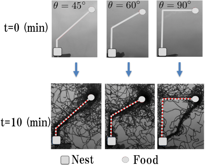
Figure 1: Three types of experimental settings and results of observed paths of ants reported by the Nishimori group.

1.  At the beginning of each experiment, the preliminarily extracted recruit pheromone was applied along one of the three kinds of polygonal lines connecting the nest and the food source, which we will call the ‘pheromone road’ in this paper. There one folding point was included in the lines with the turning angles $\theta\in\{45^{\circ},60^{\circ},90^{\circ}\}$ (see Fig.1). The preliminarily extracted pheromone has a sufficiently high density to keep strong attraction of ants until the end of each experiment.

2.  It is considered from another experiment of the Nishimori group that Lasius Japonicus can figure out the landmark at the distance of the order of 10 cm [11]. Hence ants in the present setup will be able to recognize the nest direction from the food source. This direction along the optimal path from the food source to the nest is different from the direction from the food sources indicated by the ‘pheromone road’ as mentioned above.

After getting food at the food source, ants start homing walk, and a conflict between the direction along the ‘pheromone road’ and the straight direction to the nest required ants to make decision on which they rely chemical cues or visual cues. The degree $\alpha$ of this conflict becomes larger as the angle $\theta$ increases.

Figure 1 shows the results. In the upper pictures, the initially prepared ‘pheromone roads’ are indicated by light-gray lines, each of them have a folding point with turning angle $\theta=45^{\circ},60^{\circ}$, and $90^{\circ}$, respectively. Lower pictures show trajectories of foraging ants recorded during the middle time period (about 10 min) of each experiment with duration 60 min. Only in the case of $\theta=90^{\circ}$, a direct path between the nest and the food source was established, whereas in other cases, no direct path was established until the end of experiment at time $t=60$ min.

It was claimed [10] that the change of the dominant path from trailing paths of the ‘pheromone road’ to the direct path did not associate with a continuous geometrical change of path, and instead, the direct path spontaneously emerged only in the case of $\theta=90^{\circ}$.

The above observation in experiments suggests that, if we introduce suitable parameters which control individual motion of ants, there are critical values of parameters and the change of dominant path can occur only in the ‘supercritical regime’ of parameters. In the present paper, we introduce two kinds of order parameters characterizing global changes of path patterns of foraging ants in homing walks from the food source to the nest. Roughly speaking, they are given by

$$M =\frac{\sharp\{\mbox{pioneering ants and their followers}\}}{\sharp\{\mbox{homing ants}\}},$$

$$\widetilde{M} =\frac{\sharp\{\mbox{ants trailing the `pheromone road'}\}}{\sharp\{\mbox{homing ants}\}},$$ (1.3)

where $\sharp\{\mbox{elements}\}$ denotes the total number of elements in a set $\{\mbox{elements}\}$. The precise definition of $M$ and $\widetilde{M}$ will be given in Section 3. We will discuss the possibility to regard the global changes of path patterns as continuous phase transitions associated with critical phenomena [1, 9, 12].

2 Discrete-time Stochastic Model on a Square Lattice

2.1 Switching random walks interacting through pheromone field

[General setting]   Consider an $(L-1)\times(L-1)$ square region on a square lattice. The set of vertices (sites) is given by

$$V_{L}:=\{v=(x,y):x\in\{0,1,\dots,L-1\},y\in\{0,1,\dots,L-1\}\}.$$ (2.1)

We write the Euclidean distance between two vertices $v_{1},v_{2}\in V_{L}$ as $|v_{1}-v_{2}|$.

With discrete time

$$t\in\mathbb{N}_{0}:=\{0,1,\dots\},$$ (2.2)

we consider a set of random walks of a given number of particles, $N\in\mathbb{N}:=\{1,2,\dots\}$, on $V_{L}$. They are interacting with each other through a time-dependent pheromone field as explained below. We do not impose, however, any exclusive interaction between particles. Hence each vertex $v\in V_{L}$ can be occupied by any number of particles at each time.

The nest and food source are assumed to be located at the origin $v_{\rm n}:=(0,0)$ and at the most upper-right vertex $v_{\rm f}:=(L-1,L-1)$, respectively.

All particles start from $v_{\rm n}$ at $t=0$ and perform drifted walk toward $v_{\rm f}$. After arriving at $v_{\rm f}$, each particle immediately starts drifted walk from $v_{\rm f}$ toward $v_{\rm n}$ and then returns to $v_{\rm n}$. In this way, particles shuttle between $v_{\rm n}$ and $v_{\rm f}$ for a given time period $T$. When the particle is in a time period for walking from $v_{\rm n}$ to $v_{\rm f}$, we say that it is in an exploring-period, and when it is in a time period for walking from $v_{\rm f}$ to $v_{\rm n}$, it is said to be in a homing-period.

We will denote the two types of hopping rules, which represent the slow mode and the fast mode of the drifted random walk, respectively. The particles are labeled by $j=1,\dots,N$. At each time $t\in\mathbb{N}_{0}$, the state of a particle is specified by

$$\mbox{the location}:\,\,v\in V_{L},$$

$$\mbox{and the types of hopping : the slow mode (s) or the fast mode (f)}.$$

Hence, at each time $t\in\mathbb{N}_{0}$, the $N$-particle configuration is given by a set

$$X(t):=\{X_{j}(t):j=1,\dots,N\}$$ (2.3)

of pairs of random variables:

$$X_{j}(t)=(v_{j}(t),\sigma_{j}(t)),\quad v_{j}(t)\in V_{L},\quad\sigma_{j}(t)\in\{{\rm s},{\rm f}\},$$ (2.4)

$j=1,\dots,N$. We will define a discrete-time stochastic process $(X(t))_{t\in\mathbb{N}_{0}}$.

[Time-dependent pheromone field]

The pheromone is put on vertices and its intensity is expressed by a nonnegative integer,

$$f(v,t)\in\mathbb{N}_{0},\quad v\in V_{L},\quad t\in\mathbb{N}_{0}.$$ (2.5)

That is, $f(v,t)=f\in\mathbb{N}_{0}$ means that there are $f$ units of pheromone on the vertex $v\in V_{L}$ at time $t\in\mathbb{N}_{0}$. Define the $\Gamma$-shaped subset of $V_{L}$,

$$\Gamma_{L,\ell}= \{(x,y)\in V_{L}:0\leq x\leq\ell-1,0\leq y\leq L-1\}$$

$$\cup\{(x,y)\in V_{L}:0\leq x\leq L-1,L-\ell\leq y\leq L-1\}.$$ (2.6)

We will call $\Gamma_{L,\ell}$ the $\Gamma$-region, which represents the ‘pheromone road’. The variable $\ell$ indicates the width of the $\Gamma$-region. See Fig.2.

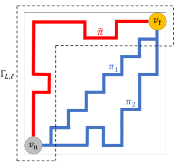
Figure 2: Setting of the model on the square region $V_{L}$ is illustrated. Paths from the food source $v_{\rm f}$ to the nest $v_{\rm n}$ in the homing-period are classified. The path $\widetilde{\pi}$ shown by a red line is an example of $\Gamma$-path which is completely included in the $\Gamma$-region, $\Gamma_{L,\ell}$. Two examples of nearly-optimal-paths are given by $\pi_{1}$ and $\pi_{2}$ drawn by blue lines. Some parts of paths are outside of $\Gamma_{L,\ell}$ and each homing duration $A$ satisfies $2(L-1)\leq A\leq 2(L-1)+\langle\Delta A_{0}\rangle/2$.

With a parameter $f_{0}\in\mathbb{N}$, the initial value of the pheromone field is given by

$$f(v,0)=\begin{cases}f_{0},&\mbox{if $v\in\Gamma_{L,\ell}$},\cr 0,&\mbox{if $v\in V_{L}\setminus\Gamma_{L,\ell}$},\end{cases}$$ (2.7)

where $V_{L}\setminus\Gamma_{L,\ell}$ denotes the complement of $\Gamma_{L,\ell}$ in $V_{L}$. With parameters $f_{1},f_{2}\in\mathbb{N}_{0}$, for each arrival of a particle at each vertex $v\in V_{L}$, secretion of pheromone by an ant is represented by the following increment of the intensity,

$$f\to\begin{cases}f+f_{1},&\mbox{in an exploring-period},\cr f+f_{2},&\mbox{in a homing-period}.\end{cases}$$ (2.8)

If $v\in V_{L}\setminus\Gamma_{L,\ell}$, each unit of pheromone evaporates with probability $q$ independently at each time step $t\to t+1$. That is, at the time step $t\to t+1$,

$$f\to f-n\quad\mbox{with probability}\quad\binom{f}{n}q^{n}(1-q)^{f-n},\quad n=0,1,\dots,f.$$ (2.9)

If $v\in\Gamma_{L,\ell}$, however, only excess of $f$ over $f_{0}$ evaporates. That is, if and only if $f>f_{0}$,

$$f\to f-n\quad\mbox{with probability}\quad\binom{f-f_{0}}{n}q^{n}(1-q)^{f-f_{0}-n},\quad n=0,1,\dots,f-f_{0}.$$ (2.10)

[Hopping rule in an exploring-period]   When ants are in an exploring-period, they are all in the slow mode; $\sigma_{j}(t)\equiv{\rm s}$. For $X_{j}(t)=(v_{j}(t),{\rm s})$, we define a set of the nearest-neighboring vertices of $v_{j}(t)$ as

$$\Lambda^{\rm s}_{j}(t) :=\begin{cases}\{v\in V_{L}:|v-v_{j}(t)|=1\}=\{(1,0),(0,1)\},&\mbox{if $v_{j}(t)=v_{\rm n}$},\cr\{v\in V_{L}:|v-v_{j}(t)|=1,v\not=v_{j}(t-1)\},&\mbox{if $v_{j}(t)\in V_{L}\setminus\{v_{\rm n}\}$}.\end{cases}$$ (2.11)

Then at each time step $t\to t+1$,

$$v_{j}(t)\to v\quad\mbox{with probability}\quad\frac{f(v,t)}{\sum_{w\in\Lambda^{\rm s}_{j}(t)}f(w,t)},\quad\mbox{if and only if $v\in\Lambda^{\rm s}_{j}(t)$},$$ (2.12)

provided that $\sum_{w\in\Lambda^{\rm s}_{j}(t)}f(w,t)>0$. If $\sum_{w\in\Lambda^{\rm s}_{j}(t)}f(w,t)=0$; that is, $f(v,t)=0$ for all $v\in\Lambda^{\rm s}_{j}(t)$, then

$$v_{j}(t)\to v\quad\mbox{with probability}\quad\frac{1}{|\Lambda_{j}^{\rm s}(t)|},\quad\mbox{if and only if $v\in{\Lambda}^{\rm s}_{j}(t)$},$$ (2.13)

where $|\Lambda_{j}^{\rm s}(t)|$ denotes the total number of vertices in $\Lambda^{\rm s}_{j}(t)$. Notice that the previous position $v_{j}(t-1)$ is not included in $\Lambda^{\rm s}_{j}(t)$ in order to forbid backward walking.

(Prohibition against cyclic motions) In an exploring-period, if $v_{j}(t+1)-v_{j}(t)\in\{(-1,0),(0,-1)\}$, that is, the step is leftward or downward, the hopping is regarded as a retrograde motion. We prohibit any succession of such retrograde motions in order to avoid cyclic motions of walkers. When the particle is in the domain $\Gamma_{L,\ell}$, this prohibition rule is strengthened so that all downward steps are forbidden, if $0\leq x\leq\ell-1$, and all leftward steps are forbidden, if $L-\ell\leq y\leq L-1$.

[Hopping rules in a homing-period]

(Slow mode)   For $X_{j}(t)=(v_{j}(t),{\rm s})$ in a homing-period, we define a set of the nearest-neighboring vertices of $v_{j}(t)$ as

$$\widetilde{\Lambda}^{\rm s}_{j}(t) :=\begin{cases}\{v\in V_{L}:|v-v_{j}(t)|=1,v\not=v_{j}(t-1)\},\cr\hskip 142.26378pt\mbox{if $v_{j}(t)\in V_{L}\setminus\{v_{\rm f}\}$},\cr\{v\in V_{L}:|v-v_{j}(t)|=1\}=\{(L-2,L-1),(L-1,L-2)\},\cr\hskip 142.26378pt\mbox{if $v_{j}(t)=v_{\rm f}$}.\end{cases}$$ (2.14)

Notice that the previous position $v_{j}(t-1)$ is not included in $\widetilde{\Lambda}^{\rm s}_{j}(t)$ also in order to forbid backward walking. Then at each time step $t\to t+1$,

$$v_{j}(t)\to v\quad\mbox{with probability}\quad\frac{f(v,t)}{\sum_{w\in\widetilde{\Lambda}^{\rm s}_{j}(t)}f(w,t)}.\quad\mbox{if and only if $v\in\widetilde{\Lambda}^{\rm s}_{j}(t)$},$$ (2.15)

provided that $\sum_{w\in\widetilde{\Lambda}^{\rm s}_{j}(t)}f(w,t)>0$. If $\sum_{w\in\widetilde{\Lambda}^{\rm s}_{j}(t)}f(w,t)=0$; that is, $f(v,t)=0$ for all $v\in\widetilde{\Lambda}^{\rm s}_{j}(t)$, then

$$v_{j}(t)\to v\quad\mbox{with probability}\quad\frac{1}{|\widetilde{\Lambda}_{j}^{\rm s}(t)|},\quad\mbox{if and only if $v\in\widetilde{\Lambda}^{\rm s}_{j}(t)$}.$$ (2.16)

(Prohibition against cyclic motions) In a homing-period, if $v_{j}(t+1)-v_{j}(t)\in\{(1,0),(0,1)\}$, that is, the step is rightward or upward, the hopping is regarded as a retrograde motion. We prohibit any succession of such retrograde motions in order to avoid cyclic motions of walkers. When the particle is in the domain $\Gamma_{L,\ell}$, this prohibition rule is strengthened so that all rightward steps are forbidden, if $L-\ell\leq y\leq L-1$, and all upward steps are forbidden, if $0\leq x\leq\ell-1$.

(Fast mode)   For $X_{j}(t)=(v_{j}(t),{\rm f})$ in a homing-period, we define a subset of the nearest-neighboring vertices of $v_{j}(t)$ as

$$\widetilde{\Lambda}^{\rm f}_{j}(t):=\{v\in V_{L}:|v-v_{j}(t)|=1,|v|<|v_{j}(t)|\}.$$ (2.17)

Then in the time step $t\to t+1$,

$$v_{j}(t)\to v\quad\mbox{with probability}\quad\frac{1}{|\widetilde{\Lambda}_{j}^{\rm f}(t)|},\quad\mbox{if and only if $v\in\widetilde{\Lambda}^{\rm f}_{j}(t)$}.$$ (2.18)

Note that since we have considered the system in a subset $V_{L}$ of the square lattice, $|\widetilde{\Lambda}^{\rm f}_{j}(t)|\in\{1,2\}$. If $x=0$ or $y=0$ in $v_{j}(t)=(x,y)$, $|\widetilde{\Lambda}^{\rm f}_{j}(t)|=1$, and hence, the hopping of the fast mode is deterministic.

(Switching)   We introduce parameters $\gamma_{\rm sf},\gamma_{\rm fs}\in[0,1]$. Then in the time step $t\to t+1$ in a homing-period, we change the mode of hopping as

$$\sigma_{j}(t) ={\rm s}\to{\rm f}\quad\mbox{with probability $\gamma_{\rm sf}$},$$

$$\sigma_{j}(t) ={\rm f}\to{\rm s}\quad\mbox{with probability $\gamma_{\rm fs}$}.$$ (2.19)

It means that the mode is not changed with probability $1-\gamma_{\rm sf}$ (resp. $1-\gamma_{\rm fs}$), when the particle is in the slow (resp. fast) mode at each time.

[Initial condition, update rule, random switching at food source, and time duration]

(i)   We start from the initial configuration such that all $N$ particles are in the slow mode and at the origin,

$$X_{j}(0)=(0,{\rm s}),\quad j=1,\dots,N.$$ (2.20)

(ii)   We perform hopping of particles and switching of the mode in a homing-period sequentially according to the numbering of particles $j=1,\dots,N$. The update of the pheromone field is done at each time step.

(iii)   When $v_{j}(t)=v_{\rm f}$, that is, an ant arrives at the food source, switching between the slow mode and the fast mode is randomly occurs:

$$\sigma_{j}(t+1)=\begin{cases}{\rm s},&\mbox{with probability 1/2},\cr{\rm f},&\mbox{with probability 1/2}.\end{cases}$$ (2.21)

(iv)   Let $\tau(n)$ be the time duration so that the total number of particles which have returned to the nest $v_{\rm n}$ at least once is $n$. We perform each numerical simulation up to time step

$$T=\tau(\kappa N),$$ (2.22)

where $\kappa$ is a parameter. That is, during $T$, totally $\kappa N$ particles shuttle between the nest and the food source.

2.2 Parameter setting

We set the parameters concerning the time-dependent pheromone field as

$$f_{0}=1000,\quad f_{1}=0,\quad f_{2}=10,\quad q=0.01.$$ (2.23)

We assume that the density of particles is fixed to be

$$\rho:=\frac{N}{L^{2}}=\frac{1}{8}=0.125,$$ (2.24)

the ratio of the width of the $\Gamma$-region defined by (2.6) with respect to $L$ is given by

$$\frac{\ell}{L}=\frac{1}{20},$$ (2.25)

and each simulation is done for the time duration (2.22) with

$$\kappa=4.$$ (2.26)

We have performed the numerical simulation of the present stochastic model on the square lattices with sizes $L=40$, $60$, and $80$. In the present paper, we will report the dependence of the simulation results on the switching parameters $\gamma_{\rm sf}$ and $\gamma_{\rm fs}$ which are changed in the interval $[0,1]$. We have confirmed that the numerical results given below are not changed qualitatively by changing the parameter setting (2.23)–(2.26). In particular, the setting (2.26) for the time duration of each simulation is sufficient to observe stable distributions of homing duration, which will be reported in Section 3. The validity of the $L$-dependence of parameters (2.24) and (2.25) will be discussed in Section 4.1. Systematic study of quantitative dependence of the model on the other parameters than $L,\ell,N$ and $\gamma_{\rm sf}$ (with the relation $\gamma_{\rm fs}=1-\gamma_{\rm sf}$) is considered as one of the future problems as discussed in the item (v) in Section 5. Table 1 summarizes the setting, changing, and fixed parameters of the present model.

Table 1: List of the setting, changing, and fixed parameters in the present discrete-time stochastic model on a square lattice

setting parameters		setting
$L$	system size	40, 60, 80
$\ell$	width of the $\Gamma$-region	$L/20$
$N$	number of particles	$\rho L^{2}=L^{2}/8$
changing parameters		range of value
$\gamma_{\rm sf}$	switching probability from slow mode to fast mode	$[0,1]$
$\gamma_{\rm fs}$	switching probability from fast mode to slow mode	$[0,1]$ or $1-\gamma_{\rm sf}$
fixed parameters		value
$f_{0}$	initial intensity of pheromone in the $\Gamma$-region	1000
$f_{1}$	amount of pheromone dropped by an exploring particle	0
$f_{2}$	amount of pheromone dropped by a homing particle	10
$q$	evaporation rate of pheromone	0.01
$\kappa$	time duration of simulation $T=\tau(\kappa N)$	4

3 Distributions of Homing Duration and Order Parameters

3.1 $\Gamma$-paths and order parameter $\widetilde{M}$

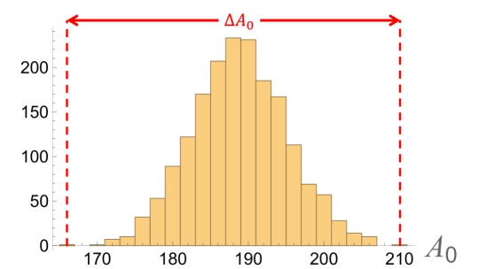
Figure 3: Histogram of the homing duration $A_{0}$ of particles in one sample of simulation, when $(\gamma_{\rm sf},\gamma_{\rm fs})=(0,1)$, in the system with size $L=60$. All particles are in the slow mode and trail $\Gamma$-paths. In this observed distribution, mean of $A_{0}$ is $188.9$, the maximum and minimum values are 210 and 166, respectively, and then $\Delta A_{0}=44$.

For each particle in the homing-period, we trace the path from the food source $v_{\rm f}$ to the nest $v_{\rm n}$,

$$\pi=\{v_{\rm f}=v_{0}\to v_{1}\to v_{2}\to\cdots\to v_{A}=v_{\rm n}\}.$$ (3.1)

Here the number of steps in $\pi$ indicating the path length is expressed by $A$. In the present paper, we call this random variable $A$ the homing duration.

First we consider the extreme case with $\gamma_{\rm sf}=0$ and $\gamma_{\rm fs}=1$. In this case all particles are in the slow mode following the ‘pheromone road’. Hence all paths in the homing-period are completely included in the $\Gamma$-region, $\Gamma_{L,\ell}$, defined by (2.6). In general, if the path in the homing-period is completely included in the $\Gamma$-region, then we say that the path is a $\Gamma$-path. (See Fig.2.) In this extreme case, we write the random variable of homing duration as $A_{0}$ by putting subscript 0. Figure 3 shows a typical distribution of homing duration $A_{0}$ in one sample of simulation for the system with size $L=60$. We notice that the minimal value of the homing duration is $2(L-1)=118$, which is realized by a $\Gamma$-shaped homing walk along the uppermost edges and then the leftmost edges of the square lattice. The observed distribution of $A_{0}$ in this simulation is, however, centered at a larger value $\simeq 189$. It means that the slow mode paths are far from optimal and include many redundant walks which are enhanced by the pheromone field. In the observed distribution, we measured the width $\Delta A_{0}$ defined by the difference between the observed maximum and minimum values of $A_{0}$. We calculated the averaged value $\langle\Delta A_{0}\rangle$ over several samples of numerical simulation. The results are the following:

$$\langle\Delta A_{0}\rangle =26.6\pm 1.8,\quad\mbox{for $L=40$}$$

$$\langle\Delta A_{0}\rangle =41.6\pm 2.7,\quad\mbox{for $L=60$}$$

$$\langle\Delta A_{0}\rangle =54.4\pm 3.2,\quad\mbox{for $L=80$},$$ (3.2)

where the errors are given by the standard deviations over ten samples of numerical simulation for the systems with sizes $L=40$ and $60$, and five samples for the system with size $L=80$. The above results show a linear dependence of $\langle\Delta A_{0}\rangle$ on size $L$,

$$\langle\Delta A_{0}\rangle\simeq 0.7L-0.83,$$ (3.3)

as shown by Fig.4.

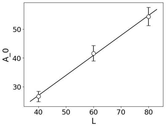
Figure 4: Dependence of $\langle\Delta A_{0}\rangle$ on $L$ is well described by a linear fitting; $\langle\Delta A_{0}\rangle\simeq 0.7L-0.83$. The errors are given by the standard deviations over ten samples of numerical simulation for the systems with sizes $L=40$ and $60$, and five samples for the system with size $L=80$.

We define $\widetilde{M}$ by the ratio of the number of observed particles following $\Gamma$-paths to the total number of homing particles in simulation; i.e. $\kappa N=\kappa L^{2}/8$ ;

$$\widetilde{M}:=\frac{\sharp\{\mbox{homing particle following a $\Gamma$-path}\}}{\kappa N}.$$ (3.4)

As mentioned above, $\widetilde{M}=1$, if $(\gamma_{\rm sf},\gamma_{\rm fs})=(0,1)$.

From now on we assume the relation

$$\gamma_{\rm sf}+\gamma_{\rm fs}=1.$$ (3.5)

As $\gamma_{\rm sf}$ increases from 0, $\widetilde{M}$ will decrease from 1, since particles in the fast mode appear and they make deviation from the ‘pheromone road’. In other words, $\widetilde{M}$ will play a role of the order parameter for the path selection which persists the original ‘pheromone road’ in the homing-period.

3.2 Nearly-optimal-paths and order parameter $M$

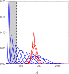
(a) Dependence on $\gamma_{\rm sf}$ with the relation $\gamma_{\rm fs}=1-\gamma_{\rm sf}$ of the distributions of homing duration $A$ of $\Gamma$-paths (shown by red curves) and of non-$\Gamma$-paths (by blue curves) for the system with $L=60$. Three distributions of $A$ are shown for the $\Gamma$-paths with $\gamma_{\rm sf}=0$, $0.1$, and $0.2$, and ten for the non-$\Gamma$-paths with $\gamma_{\rm sf}=0.1$, $0.2$, $0.3$, $0.4$, $0.5$, $0.6$, $0.7$, $0.8$, $0.9$, and $1$. In both cases, the right edge (the point at which the right tail of distribution becomes zero) decreases monotonically as $\gamma_{\rm sf}$ increases.

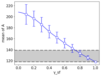
(b) Means of the distribution of $A$ for the non-$\Gamma$-paths (shown by the blue curves in (a)) are plotted versus $\gamma_{\rm sf}\in(0,1]$. The standard deviations of distribution of $A$ are shown by the error bars.

Figure 5: Distributions of homing duration $A$. The shaded region indicates the range of $A$, $2(L-1)\leq A\leq 2(L-1)+\langle\Delta A_{0}\rangle/2$, for the nearly-optimal-paths. For $L=60$, $2(L-1)=118$ and $\langle\Delta A_{0}\rangle/2=20.8$ by (3.2).

For the system with size $L=60$, Fig. 5 (a) shows the dependence of the distribution of homing duration $A$ on $\gamma_{\rm sf}$ with the relation (3.5). When $\gamma_{\rm sf}\gtrsim 0.3$, $\Gamma$-path is not observed any more and observed paths are dominated by non-$\Gamma$-paths. As $\gamma_{\rm sf}$ increases, the observed support of distribution of homing duration for the non-$\Gamma$-paths shifts to the lower-valued region of $A$. It means that as $\gamma_{\rm sf}$ increases, more pioneer walkers appear who build shorter paths from the food source to the nest, since particles can be in the fast mode more frequently. In addition to the shift to the left, we also see in Fig. 5 (a) that the bell-shaped distribution of $A$ for the the non-$\Gamma$-paths becomes sharper as $\gamma_{\rm sf}$ increases. Monotonic decrease of the mean $\langle A\rangle$ and the standard deviation $\sigma$ of the distribution of $A$ as the increment of $\gamma_{\rm sf}$ is shown by Fig. 5 (b) for the non-$\Gamma$-paths. This implies that the shorter paths are strengthened by followers of pioneer walkers via the interaction through pheromone field. As $\gamma_{\rm sf}$ approaches to 1, the distribution quickly sharpens and seems to be condensed to the shortest value of $A$, i.e. the length of the optimal path, $2(L-1)=118$. In other words, as $\gamma_{\rm sf}$ approaches to 1, a large amount of particles tend to trail the paths which are very near to the optimal path. We want to call such paths the nearly-optimal-paths.

In order to define the nearly-optimal-paths, we use the value $\langle\Delta A_{0}\rangle$ determined by the homing-duration distribution when $(\gamma_{\rm sf},\gamma_{\rm fs})=(1,0)$ in Section 3.1. That is, if the homing duration $A$ of the path satisfies the condition

$$2(L-1)\leq A\leq 2(L-1)+\frac{1}{2}\langle\Delta A_{0}\rangle,$$ (3.6)

then we say that it is a nearly-optimal-path. This range (3.6) of $A$ is indicated by a shaded region in Figs. 5 (a) and (b). Then we define another order parameter $M$ in addition to $\widetilde{M}$ by the ratio of the number of particles following nearly-optimal-paths in a homing-period to the total number of homing particles in simulation, $\kappa N$,

$$M:=\frac{\sharp\{\mbox{homing particle following a nearly-optimal-path}\}}{\kappa N}.$$ (3.7)

Figure 2 illustrates an example of $\Gamma$-path which contributes to the order parameter $\widetilde{M}$ and two examples of nearly-optimal-paths which contribute to the order parameter $M$. We will compare the dependence on $\gamma_{\rm sf}$ of these two kinds of order parameters $M$ and $\widetilde{M}$ with changing the system size $L$. The choice of $\langle\Delta A_{0}\rangle/2$ as a width in the condition (3.6) which defines the nearly-optimal-paths is to make the dependence of $M$ on $L$ be comparable with that of $\widetilde{M}$. The definitions (3.6) and (3.7) work well as shown below.

4 Phase Transitions and Critical Phenomena in Path Selections

4.1 Almost data-collapse with respect to system size

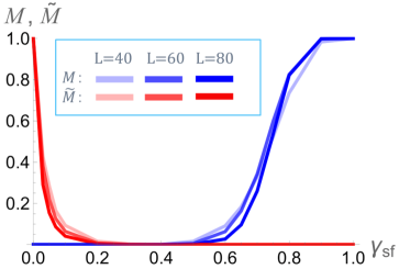
(a) Numerical results of $M_{L}$ and $\widetilde{M}_{L}$ for the finite systems with sizes $L=40$, $60$, and $80$.

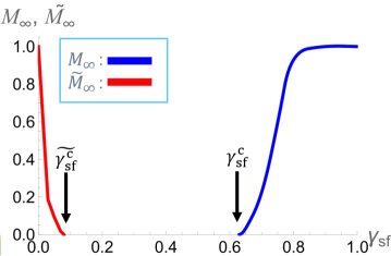
(b) $M_{\infty}$ and $\widetilde{M}_{\infty}$ for the infinite system estimated by the $1/L$-plots as explained in Section 4.2. The critical values $\gamma_{\rm sf}^{\rm c}\simeq 0.63$ and $\widetilde{\gamma_{\rm sf}^{\rm c}}\simeq 0.08$ estimated there are indicated by arrows.

Figure 6: Order parameters $M$ and $\widetilde{M}$ are plotted versus $\gamma_{\rm sf}\in[0,1]$, where $\gamma_{\rm fs}=1-\gamma_{\rm sf}$.

With the relation between parameters (3.5), Fig.6 (a) shows the $\gamma_{\rm sf}$-dependence of the two kinds of order parameters, $M$ and $\widetilde{M}$, for the systems with different sizes, $L=40$, $60$, and $80$. For the systems with sizes $L=40$, $60$, (resp. $80$) we have obtained 10 samples (resp. 3 samples) for each parameter $\gamma_{\rm sf}\in[0,1]$. The lines interpolate the averaged values of these samples. We have confirmed that the standard deviations are very small, e.g. $3.0\times 10^{-3}$ for $M$ at $\gamma_{\rm sf}=0.6$ and $1.5\times 10^{-2}$ for $\widetilde{M}$ at $\gamma_{\rm sf}=0.1$ for $L=60$, and hence error bars are omitted in Fig.6 (a). By definition, $\widetilde{M}\to 1$ as $\gamma_{\rm sf}\to 0$, and $M\to 1$ as $\gamma_{\rm sf}\to 1$. We see that when $\gamma_{\rm sf}$ is small, $M=0$ and $\widetilde{M}>0$, while when $\gamma_{\rm sf}$ is large, $M>0$ and $\widetilde{M}=0$. The rapid decrease of $\widetilde{M}$ around $\gamma_{\rm sf}\simeq 0.1$, and the rapid increase of $M$ around $\gamma_{\rm sf}\simeq 0.6$ indicate the global switching phenomena of path selections between the $\Gamma$-paths and the nearly-optimal-paths.

Figure 6 (a) shows that the differences of the values of $M$ and $\widetilde{M}$ caused by enlarging the system size $L$ are relatively small. Roughly speaking, this fact will be regarded as a kind of data collapse, which shows independence of the global switching phenomena in path selections on the size $L$ in the present model. In other words, our settings of the number of particles, $N=\rho L^{2}\propto L^{2}$, given by (2.24), the width of the $\Gamma$-region (‘pheromone road’), $\ell=L/20\propto L$, given by (2.25), and the condition (3.6) for the nearly-optimal-paths using the quantity, $\langle\Delta A_{0}\rangle\simeq aL+b$, (see (3.3)) are very simple but they provide a proper scaling property of the system with respect to the change of the system size $L$.

4.2 Evaluations of critical values and critical exponents

On the other hand, in the vicinity of the values of $\gamma_{\rm sf}$ at which $\widetilde{M}$ approaches zero ($\gamma_{\rm sf}\simeq 0.1$) and at which $M$ emerges ($\gamma_{\rm sf}\simeq 0.6$), the changes show systematic dependence on $L$. This observation suggests that we will have critical phenomena in the $L\to\infty$ limit and the present global switching phenomena in path selections can be considered as continuous phase transitions.

In order to explain our method to estimate the order parameters in the $L\to\infty$ limit, here we write the order parameters as $M_{L}$ and $\widetilde{M}_{L}$ for the system with size $L$. We assume the following simple dependence of the order parameters on the system size $L$,

$$M_{\infty}=M_{L}+\frac{c_{1}}{L},\quad\widetilde{M}_{\infty}=\widetilde{M}_{L}+\frac{\widetilde{c_{1}}}{L},\quad\mbox{as $L\to\infty$},$$ (4.1)

where $c_{1}$ and $\widetilde{c_{1}}$ are fitting parameters, and $M_{\infty}$ and $\widetilde{M}_{\infty}$ are the estimated values of the order parameters for the infinite system. (See the item (ii) in Section 5 for a possible improvement by introducing a critical exponent $\nu$.) Then if we plot the values of $M_{L}$ (resp. $\widetilde{M}_{L}$) with respect to $1/L$, the $L\to\infty$ limit of order parameter $M_{\infty}$ (resp. $\widetilde{M}_{\infty}$) will be evaluated by the ‘$y$-intercept’. The estimated curves of $M_{\infty}$ and $\widetilde{M}_{\infty}$ are shown for $\gamma_{\rm sf}\in[0,1]$ in Fig. 6 (b).

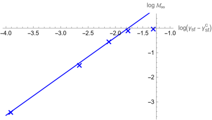
(a) Fitting with $\gamma_{\rm sf}^{\rm c}=0.63$ and $\beta=1.59$ for $M_{\infty}$.

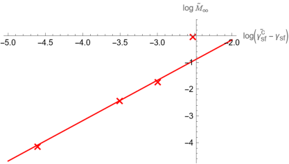
(b) Fitting with $\widetilde{\gamma_{\rm sf}^{\rm c}}=0.08$ and $\widetilde{\beta}=1.51$ for $\widetilde{M}_{\infty}$.

Figure 7: Log-log plots of the order parameters $M_{\infty}$ and $\widetilde{M}_{\infty}$ with respect to the deviations of the parameter $\gamma_{\rm sf}$ from its critical values, $\gamma_{\rm sf}-\gamma_{\rm sf}^{\rm c}$ and $\widetilde{\gamma_{\rm sf}^{\rm c}}-\gamma_{\rm sf}$, respectively. The slopes give the critical exponents $\beta$ and $\widetilde{\beta}$.

The results suggest that we can define the two kinds of critical values of $\gamma_{\rm sf}$ according to the two kinds of order parameters, $M_{\infty}$ and $\widetilde{M}_{\infty}$, as

$$\gamma_{\rm sf}^{\rm c}:=\inf\{\gamma_{\rm sf}:M_{\infty}>0\},\quad\widetilde{\gamma_{\rm sf}^{\rm c}}:=\sup\{\gamma_{\rm sf}:\widetilde{M}_{\infty}>0\}.$$ (4.2)

From the $1/L$-plots, we have evaluated the critical values as

$$\gamma_{\rm sf}^{\rm c}\simeq 0.63,\quad\widetilde{\gamma_{\rm sf}^{\rm c}}\simeq 0.08.$$ (4.3)

See Fig. 6 (b).

The continuous changes of $M$ and $\widetilde{M}$ at these critical points suggest that the phase transitions are continuous. Then the critical phenomena will be described by the following power laws as the functions of the parameter $\gamma_{\rm sf}$,

$$M_{\infty}(\gamma_{\rm sf}) \simeq c_{2}(\gamma_{\rm sf}-\gamma_{\rm sf}^{\rm c})^{\beta},\quad\gamma_{\rm sf}\gtrsim\gamma_{\rm sf}^{\rm c},$$

$$\widetilde{M}_{\infty}(\gamma_{\rm sf}) \simeq\widetilde{c_{2}}(\widetilde{\gamma_{\rm sf}^{\rm c}}-\gamma_{\rm sf})^{\widetilde{\beta}},\quad\gamma_{\rm sf}\lesssim\widetilde{\gamma_{\rm sf}^{\rm c}},$$ (4.4)

where $\beta$ and $\widetilde{\beta}$ are the critical exponents of order parameters $M$ and $\widetilde{M}$, respectively [1, 9, 12]. As shown by Fig.7, the power laws are observed and the log-log plots give the values

$$\beta\simeq 1.6,\quad\widetilde{\beta}\simeq 1.5.$$ (4.5)

5 Concluding Remarks and Future Problems

At the end of this paper, we list out the concluding remarks and possible future problems.

(i)  The interactions between ants are given through the pheromone field, which evolves in time affected by the previous behaviors of other ants. In the present study, we have studied such an interacting particle system by numerically simulating a cellular automaton model. What kind of theory is relevant to describe such kind of temporally inhomogeneous interaction with memory effects?

(ii)  In the finite-size scaling theory [1, 9, 12], the $1/L$-fitting (4.1) should be refined by introducing exponents $\nu$ and $\widetilde{\nu}$ as

$$M_{\infty}=M_{L}+\frac{c_{1}}{L^{\nu}},\quad\widetilde{M}_{\infty}=\widetilde{M}_{L}+\frac{\widetilde{c_{1}}}{L^{\widetilde{\nu}}},\quad\mbox{as $L\to\infty$}.$$ (5.1)

In the present study, we have obtained numerical results for only three sizes $L=40$, $60$, and $80$. Hence it is rather difficult to evaluate the values of $\nu$ and $\widetilde{\nu}$ by numerical fitting. We have assumed the mean-field value $\nu=\widetilde{\nu}=1$ in the fitting (4.1). The obtained numerical results (4.5) suggest $\beta=\widetilde{\beta}=3/2$. Systematic study of finite-size scaling based on larger scale simulation will be an important future problem. The correlation functions and the response functions of the present model for the group behavior of ants should be carefully considered in order to understand the critical phenomena described by the critical exponents $\nu$, $\delta$, and $\gamma$.

(iii)  Any effective theory is desired to describe the phase transitions and critical phenomena in the path selections for foraging ants. As mentioned in the item (ii) above, first we will try to establish the mean-field theory. Fractional values of critical exponents suggest the emergence of fractal structures in paths of ants at the moment when the nearly-optimal-paths are first established, as well as at the moment when the ‘pheromone road’ vanishes in the path selections of ants.

(iv)  By the definition (2.19), the parameters $\gamma_{\rm sf}$ and $\gamma_{\rm fs}$ can take any values in $[0,1]$ independently. We have assumed in the present paper, however, the special relation (3.5) between these two parameters. The present study on the global switching of path selections shall be generalized to the whole parameter space $(\gamma_{\rm sf},\gamma_{\rm fs})\in[0,1]^{2}$. As a result, we will obtain the phase diagram showing three types of phases; (a) the phase in which homing particles select the $\Gamma$-paths (i.e. trailing paths of the ‘pheromone road’) indicated by $\widetilde{M}>0$ and $M=0$, (b) the phase in which homing particles select the nearly-optimal-paths indicated by $\widetilde{M}=0$ and $M>0$, and (c) the intermediate phase.

(v)  As shown by Table 1, we have fixed many parameters except $L,\ell$, $N$ and $\gamma_{\rm sf}$ with the relation (3.5). More general and systematic study of the present model will be desired by investigating the dependence of the results on other parameters. For example, if we change the parameter $\kappa$, the time duration of numerical observation is changed. Then the transient or relaxation phenomena in the initial time period and longer-term behavior of the present processes will be clarified. It will be interesting research subject to study precise dependence of the results on the evaporation rate $q$ of pheromone, since this parameter will control the spatio-temporal correlations between particles via the pheromone field.

(vi)  The present study was motivated by the experiments reported by the group of the last author (HN) of this paper as briefly explained in Section 1.2 [10]. In our modeling, we adopted the setting with $\theta=90^{\circ}$ for the turning angle of the ‘pheromone road. (See Figs. 1 and 2 again.) The reason is that any global switching phenomena in path selections was not observed in other setting with $\theta=45^{\circ}$ and $\theta=60^{\circ}$. In the present model, we have introduced other parameters $\gamma_{\rm sf}$ and $\gamma_{\rm fs}$ (the switching parameters between the fast and slow modes) and showed that the global switching phenomena in path selections are realized as continuous phase transitions associated with the critical phenomena at the critical values $\gamma_{\rm sf}^{\rm c}$ and $\widetilde{\gamma_{\rm sf}^{\rm c}}$. This result suggests that even if we adopt the setting with $\theta=45^{\circ}$ or $\theta=60^{\circ}$, we will be able to observe such phase transitions provided that we properly choose the parameters $\gamma_{\rm sf}$ and $\gamma_{\rm fs}$. In order to simulate the models with the setting with $\theta=45^{\circ}$ or $\theta=60^{\circ}$ efficiently, we shall change the lattice from the present square lattice to the triangular or the honeycomb lattices. We expect that the critical phenomena associated with the phase transitions representing the global switching phenomena in path selections are universal and do not depend on any details of the lattice structure. If so, the present study on lattice models will provide the universal statements to the path selection phenomena observed in real foraging ants.

Acknowledgements   The present authors would like to thank Mitsugu Matsushita and Hirohiko Shimada for useful discussion on the present work. This work was supported by the Research Institute for Mathematical Sciences, an International Joint Usage/Research Center located in Kyoto University. MK is supported by the Grant-in-Aid for Scientific Research (C) (No.19K03674), (B) (No.23H01077), (A) (No.21H04432), and the Grant-in-Aid for Transformative Research Areas (A) (No.22H05105) of the Japan Society for the Promotion of Science (JSPS). HN is supported by the Grant-in-Aid for Scientific Research (B) (No.20H01871), and the Grant-in-Aid for Transformative Research Areas (A) (No.21H05293) and (A) (No.21H05297) of JSPS.

References

- [1] B. Chopard, M. Droz, Cellular Automata Modeling of Physical Systems, Cambridge University Press, Cambridge, UK, 1998.
- [2] F. den Hollander, S. Nandan, Spatially inhomogeneous populations with seed-banks: I. Duality, existence and clustering, J. Theor. Probab. 35 (2022) 1792–1841.
- [3] F. den Hollander, S. Nandan, Spatially inhomogeneous populations with seed-banks: II. Clustering regime, Stochastic Process. Appl. 150 (2022) 116–146.
- [4] S. Floreani, C. Giardinà, F. den Hollander, S. Nandan, F. Redig, Switching interacting particle systems: Scaling limits, uphill diffusion and boundary layer, J. Stat. Phys. 186 (2022) 33 (45 pages).
- [5] A. Greven, F. den Hollander, M. Oomen, Spatial populations with seed-bank: Well-posedness, duality and equilibrium, Electon, J. Probab. 27 (18) (2022) 1–88.
- [6] A. Greven, F. den Hollander, M. Oomen, Spatial populations with seed-bank: Renormalisation on the hierarchical group, to appear in Memoirs of AMS. arXiv:math.PR/2110.02714
- [7] B. Hölldobler, E. O. Wilson, The Ants, Harvard University Press, Cambridge, MA, 1990.
- [8] J. T. Lennon, F. den Hollander, M. Wilke-Berenguer, J. Blath, Principle of seed banks and the emergence of complexity from dormancy, Nat. Commun. 12 (2021) 4807 (16 pages).
- [9] J. Marro, R. Dickman, Nonequilibrium Phase Transitions in Lattice Models, Cambridge University Press, Cambridge, UK, 1999.
- [10] Y. Ogihara, O. Yamanaka, T. Akino, S. Izumi, A. Awazu, H. Nishimori, Switching of primarily relied information by ants: A combinatorial study of experiment and modeling, in: (eds.) T. Ohira, T. Uzawa (Eds.), Mathematical Approaches to Biological Systems –Networks, Oscillations, and Collective Motions, Springer-Verlag, 2015, pp.119–137.
- [11] S. Shinoda, Analysis of the influence of visual cues for foraging ants (in Japanese). Graduate Thesis, Department of Mathematics, Hiroshima University, 2013.
- [12] T. Vicsek, A. Zafeiris, Collective motion. Phys. Rep. 517 (2012) 71–140.