Quantum resource theory of Bell nonlocality in Hilbert space

Abstract

We introduce a Hilbert space based resource theory of Bell nonlocality with the aim of providing bona fide measures of quantum nonlocality depending only on the intrinsic properties of the quantum states being considered. We construct our theory by defining the set of local (or free) states, i.e., the states that do not violate the Clauser-Horne-Shimony-Holt inequality; the set of free operations, i.e., the transformations that do not create the nonlocality resource, which includes local operations and shared randomness; and suitable measures of nonlocality based either on geometric distances or relative entropies with respect to the set of local states. We discuss the basic axiomatic structure that is needed for a meaningful characterization and quantification of Bell nonlocality and we illustrate the general resource theory so developed by applying it to specific classes of quantum states, including two-qubit Werner states, Bell-diagonal states, and Bell-diagonal states at fixed convexity.

I Introduction

Quantum technologies rely on tasks which cannot be performed by protocols and devices based on the principles of classical physics. Whenever we succeed in pinpointing such tasks, we next wish to know more precisely which structural aspects of quantum laws are crucial for their implementations. In other words, we try to single out prima facie quantum resources Chitambar2019 ; Theurer2021 . Fundamental traits of quantum mechanics that are identified as essential quantum technology resources and whose quantum resource theories have been developed to a great extent include: superposition Theurer2017 , steering Gallego2015 , entanglement Plenio2007 ; Horodecki2009 ; Contreras2019 , discord Dakic2012 ; Pirandola2014 , coherence Streltsov2017 , quantum incompatibility and programmability Buscemi2020 , reference frame alignment Bartlett2007 ; Gour2008 , measurement sharpness Buscemi2023 , and quantum information in nonequilibrium thermodynamics Brandao2013 ; Gour2015 . Partial resource theories of Bell nonlocality define and include resource carriers different from quantum states DeVicente2014 ; Gallego2017 .

By identifying the general framework of resource theories we can distinguish their basic elements and features Chitambar2019 ; Theurer2021 ; Kuroiwa2020 ; Gonda2023 . For each given context, we first need to determine the set of objects we recognize as resource states. Next, we need to define the set of operations on the set that are identified as low-cost or free in the given context. These two basic elements already establish a structure or even a partial ordering in the set of the resource states. Indeed, one can distinguish classes of states that are related by the free operations. The order can be established between any two states if one of them can be obtained as the result of an operation acting on the other. Finally, defining a meaningful quantification (measure) of the resource can introduce a further ordering in the set. In such circumstances one can naturally identify the null-resource states and the maximum-resource states. Additional relations between the measure and the low-cost operations can be introduced by imposing that such transformations do not generate the resource when acting on null-resource states and/or cannot increase the resource, as measured by a meaningful quantifier. When composite systems are considered, the above-mentioned elements allow for distillation of the resource; this process amounts essentially to the localization of high-quality resource states in some subsystem via free operations acting on the larger system.

These features naturally appear in the paramount instance of quantum protocols based on entanglement Ekert1991 ; Bennett1993 ; Bennett1999a ; Horodecki2009 ; Devetak2004 ; Horodecki2005 . In this case the free transformations are the local operations and classical communication (LOCC), while the null-resource states are the separable states. Depending on the specific context and the relevant operations, one can introduce several significant quantifiers of entanglement, including the von Neumann entropy of entanglement, the relative entropy of entanglement, the distillable entanglement, the distillable key, the entanglement of formation, the entanglement negativity, and the squashed entanglement Plenio2007 ; Bennett1996 ; Devetak2005 ; Christandl2006 ; Christandl2004 ; Bennett1996a ; Wootters1998 ; Eisert1999 ; Plenio2005 . In particular, when considering the Hilbert space arena, entanglement quantifications inspired by the geometry of the set of quantum states can be suitably defined in terms of contractive distances Plenio2007 ; Wei2003 ; Uyanik2010 or relative entropies Vedral1997 with respect to the set of separable states.

In the present work we show that the geometric or entropic characterizations of entanglement in Hilbert space can be extended to quantum correlations stronger than entanglement, such as Bell nonlocality Barrett2005 ; Brunner2014 ; DeVicente2014 ; Gallego2017 ; Bell1964 ; Clauser1969 ; Mermin1990 ; Ardehali1992 ; Belinskii1993 ; Laskowski2004 ; Zukowski2002 ; Weihs1998 ; Aspect1999 ; Hensen2015 . As entanglement and Bell nonlocality coincide on pure states, in this case a Hilbert-space resource theory of entanglement is automatically also a resource theory of nonlocality. On the other hand, when considering general quantum states, while Bell nonlocality always implies entanglement Brunner2014 , the converse does not necessarily hold true, the first and paramount example of entangled but local states being that of Werner states Werner1989 . Therefore, a strict hierarchy between Bell nonlocality and entanglement is established, at least for finite-dimensional systems.

In general, we say that a quantum state is nonlocal if it is possible to perform an experiment with it that cannot be equivalently described using a local hidden variable model Brunner2014 . Hence, nonlocal states associated with suitable experiments necessarily violate some form of Bell inequality on the correlations of local measurements, e.g. the Clauser-Horne-Shimony-Holt (CHSH) inequality Clauser1969 . It then appears that Bell nonlocality is not a feature of the state only, but also a property of the selected experiment. In this sense, we see the difficulty in developing a resource theory of nonlocality on equal footing with the Hilbert space-based resource theory of entanglement. Indeed, previous research on Bell nonlocality as a resource has focused on conditional probability distributions of outcomes of experiments with respect to the randomized choices of experimental setups rather than on the specific features of the quantum states involved DeVicente2014 ; Gallego2017 .

From the above discussion, we see that in order to characterize and quantify the nonlocality of a quantum state in Hilbert space one needs a criterion assessing whether there exists at least one experiment with such state that violates a Bell-type inequality. For a given quantum system, we must define and characterize the set of bipartite states that do not violate the CHSH inequality with a single copy, even after stochastic local operations without communication. Fortunately, such a general characterization exists Masanes2008 . Moreover, at least for two-qubit systems, one can also obtain a complete parameterization of the set of local states Horodecki1995 ; Masanes2008 . Thus motivated, in the present work we introduce and investigate a general quantum resource theory of Bell nonlocality in Hilbert space, in full analogy with the quantum resource theory of entanglement. In particular, we introduce and discuss the relevant axiomatic properties that need to be satisfied by set of free states and free operations, we define the entropic and geometric measures of Bell nonlocality with respect to the set of local states, we determine the structure of the maximally nonlocal states, and we study the nonlocality of several important classes of two-qubit states.

The paper is organized as follows: In Sec. II we present a general discussion of quantum resource theories, while in Sec. III we review and discuss the definition and properties of Bell nonlocality. In Sec. IV we develop the explicit Hilbert space-based resource theory of Bell nonlocality and prove some basic theorems that put it on firm grounds. Next, in Sec. V we introduce the geometric and entropic measures of Bell nonlocality defined with respect to the set of local states in Hilbert space and provide a rigorous characterization of their properties. We then move to study concrete examples: in Sec. VI we review some basic features of two-qubit states and we prove some useful theorems on the properties related to their Bell nonlocality. Using the results obtained in Sec. VI, in Sec. VII we compute explicitly the geometric and entropic measures of Bell nonlocality for various classes of two-qubit states, including Werner states, Bell-diagonal states, and fixed-convexity Bell-diagonal states. Finally, in Sec. VIII we discuss our findings and ponder about some possible future lines of investigation.

II Quantum resource theories

The fundamental role of a resource theory is to distinguish resources, or instances under which a desired performance is achieved, and free instances under which the desired performance is not achieved. Indeed, resource theories can be used to quantify a desirable quantum effect, develop new protocols for its detection, and identify processes that optimize its use for the realization of a given task. In so-called static quantum resource theories the instances are given by quantum states. A central task in resource theories is then to identify the free states, that is the states that do not carry the desired resource. The second ingredient of the theory are the transformations that do not create the resource, and thus preserve at least the free states. We name them free operations or sometimes resource non-generating transformations. There are a few general properties that free operations should satisfy Theurer2021 ; Chitambar2019 :

• Free operations preserve the set of free states.

• Their concatenation is still a free operation.

• The trivial extension of a free operation is also a free operation (as a consequence, tensor products of free operations are free operations).

• The operation of adding an auxiliary system is free.

• The operation of discarding a subsystem (partial trace) is free.

Next, we need appropriate quantifiers measuring how valuable is a given resource state. Typically, there are a few properties that a well defined quantifier should satisfy. Depending on how many of such properties are satisfied, the quantifier may be known as a resource monotone or as a full-fledged resource measure. The fundamental axiomatic properties include:

1. Faithfulness: A faithful resource quantifier must vanish if and only if the state is free.

2. Monotonicity under free operations: A resource quantifier must be monotonically non-increasing under free operations.

3. Convexity: A resource quantifier should be convex (monotonic under mixing).

4. Monotonicity under subselection: A resource quantifier must be monotonically non-increasing under subselection (quantum operations for which the measurement outcomes are retained and suitably selected).

5. Computability: A resource quantifier should be computable analytically or numerically.

A further central question in resource theories is the definition of the states carrying the maximal amount of a resource. Considering the case of bipartite entanglement for the purpose of illustration, the maximally entangled pure state is determined by showing that it is possible to deterministically obtain any other pure state from the identified maximally entangled one via the application of the free operations. In the case of entanglement, the latter are the LOCC transformations. On the other hand, the notion of maximally resourceful states is not so clear in the multipartite case and for mixed states. For example, considering entanglement again, for mixed states one needs to define the rate of distillation and the entanglement cost. This shows that conditions of convertibility under free operations are significant issues in quantum resource theories.

III Bell nonlocality

Quantum nonlocality emerges naturally in the context of Bell inequalities Bell1964 ; Clauser1969 ; Laskowski2004 . Assume two observers, Alice and Bob, with space-like separation. Alice and Bob have two different pairs of observables each of them can measure. They do not communicate. They independently choose which observable to measure and write down the results of the measurements. The correlations between the observables are chosen by both and the results obtained by both are combined to form Bell inequalities. These inequalities must be satisfied in a classical world, in which we admit at most local hidden variable models and other tacitly accepted assumptions including the independence of the choices, realism, no loopholes in experiments. For bipartite local hidden variables theories we have the following relation between the conditional probabilities of the choice of an observable $x$ by Alice and an observable $y$ by Bob, and the results of the measurement $a$ by Alice, and the measurement $b$ by Bob:

$$p(a,b|x,y)=\sum_{\lambda}p(\lambda)p(a|x,\lambda)p(b|y,\lambda),$$ (1)

where we can take

$$p(a,b|x,y)={\rm Tr}(\rho^{AB}M_{a|x}\otimes M_{b|y}).$$ (2)

Here $M_{a|x}$ is a positive operator-valued measure (POVM) for output $a$ of observable $x$, and similarly $M_{b|y}$ for output $b$ of observable $y$. It is immediate to show that for separable states Eq. (2) implies Eq. (1). Therefore, nonlocal states are certainly entangled Horodecki1995 ; Werner1989 . However, some entangled states may be local Werner1989 ; Masanes2006 ). Bell inequality in CHSH form reads:

$$E(x,y)-E(x,y^{\prime})+E(x^{\prime},y)+E(x^{\prime},y^{\prime})\leq 2,$$ (3)

where $E(x,y)$ is the statistical averages of the outcomes of measurements of $x$ and $y$ of a given quantum state. For nonlocal states Eq. (2) cannot be satisfied, and therefore CHSH inequality Eq. (3) is violated.

IV Hilbert space based resource theory of Bell nonlocality

IV.1 General aspects

Having defined the main traits of Bell nonlocality via the CHSH inequality, we now discuss the general aspects and the basic elements of the corresponding resource theory.

Free states. Free states are the local states, that is the states that do not violate the CHSH inequality Eq. (3). In the case of two-qubit systems, the set of local states can be fully characterized Horodecki1995 ; Masanes2008 and will be discussed in detail in Section VI.3 below.

Free operations. The set of the free operations is made of the local operations and shared randomness (LOSR) Chitambar2019 ; Schmid2020a . They can be defined in general as follows:

$$\int_{\lambda}d\lambda\Phi^{A}_{\lambda}\otimes\Phi^{B}_{\lambda},$$ (4)

where $\Phi^{A}_{\lambda}$ and $\Phi^{B}_{\lambda}$ are completely positive and trace preserving (CPTP) maps. These transformations cannot take a local state out of the set of local states since they leave the hidden variable model invariant. As LOSR are also LOCC (the converse is not true), they inherit many properties that are proven true for the extensively studied class of LOCC transformations. Specifically, LOSR satisfy all the properties listed in Section II: concatenations and tensor products of LOSR, as well as the trivial extensions and the partial traces all belong to the LOSR class.

Convertibility under LOSR and maximally nonlocal states. Maximally nonlocal states cannot be defined in the same sense as maximally entangled states in the resource theory of entanglement, i.e., by the property that any pure state can be obtained from the pure maximally entangled state deterministically by LOCC transformations. Indeed, classical communication is crucial in the former derivation, and this feature is not available in the case of Bell nonlocality. However, we still can think of equivalence nonlocality classes of quantum states with respect to LOSR transformations, or hierarchies inside the set of states defined as a LOSR convertibility class from a given state, i.e., the class of states that can be derived from the given state by LOSR. Pragmatically, once some valid resource monotone and/or measure has been defined, we can then identify for each measure the corresponding maximally nonlocal state by determining the state that maximizes the given measure.

IV.2 Resource monotones and measures

IV.2.1 Geometric measures

For a given quantum state $\rho$ we take as measure $\mathcal{M}(\rho)$ of Bell nonlocality any contractive distance (with the exception of the Hilbert-Schmidt distance) $D$ between $\rho$ and the closest local state $\rho_{loc}$:

$$\mathcal{M}(\rho)=\min_{\rho_{loc}\in\sigma}D(\rho,\rho_{loc})\,,$$ (5)

where $\sigma\equiv\{\rho_{loc}\}$ denotes the set of local states.

IV.2.2 Relative entropy

Relative entropy is not a distance as it does not satisfy the triangle inequality and is not symmetric with respect to state interchange, but nonetheless it is widely used in the quantum information theory and the theory of entanglement because it enjoys nearly all of the monotonicity properties that are requested in a valid quantum resource theory. The relative entropy is defined as

$$S(\rho_{1}|\rho_{2})={\rm Tr}\rho_{1}\log_{2}\rho_{1}-{\rm Tr}\rho_{1}\log_{2}\rho_{2}.$$ (6)

For states that are diagonal in the same basis with eigenvalues $e^{1}_{i}$ and $e^{2}_{i}$ respectively we have

$$S(\rho_{1}|\rho_{2})=\sum_{i}e^{1}_{i}\log_{2}e^{1}_{i}-\sum_{i}e^{1}_{i}\log_{2}e^{2}_{i}.$$ (7)

Hence, we define the measure of Bell nonlocality based on the relative entropy as

$$\mathcal{M}_{Re}(\rho)=\min_{\rho^{loc}\in\sigma}S(\rho|\rho^{loc}).$$ (8)

IV.3 Properties

Let us now investigate whether the measures introduced above satisfy the axiomatic properties listed in Section II.

• Property 1 – vanishing on free states. By definition, this property is automatically satisfied by the relative entropy and by any chosen distance.

• Property 2 – monotonicity under LOSR. For any distance $D$ that is monotonically nonincreasing under an arbitrary CPTP map $\Phi$ that preserves the locality of a local state (LOSR do satisfy this property) we have

  $$\mathcal{M}(\rho)=\min_{\rho_{loc}\in\sigma}D(\rho,\rho_{loc})=D(\rho,\rho_{loc}^{min})\geq D(\Phi(\rho),\Phi(\rho_{loc}^{min}))\geq\min_{\rho_{loc}\in\sigma}D(\Phi(\rho),\rho_{loc})=\mathcal{M}(\Phi(\rho)).$$ (9)

  It follows that any distance that is nonincreasing under CPTP maps defines a measure of nonlocality that is nonincreasing under LOSR. Property 2 holds for the relative entropy as well, since the latter is contractive under CPTP maps by construction.

• Property 3 – convexity (nonincreasing under mixing of quantum states). Since the set of local states is convex any distance that is jointly convex induces a measure of nonlocality that is convex. Denoting by $a$ the convexity parameter with $0\leq a\leq 1$, we have:

  $$a\mathcal{M}(\rho_{1})+(1-a)\mathcal{M}(\rho_{2}) = a\min_{\rho_{loc}\in\sigma}D(\rho_{1},\rho_{loc})+(1-a)\min_{\rho_{loc}\in\sigma}D(\rho_{2},\rho_{loc})$$ (10)

  $$= aD(\rho_{1},\rho_{loc}^{min})+(1-a)D(\rho_{2},\rho_{loc}^{min^{\prime}})$$ (11)

  $$\geq D(a\rho_{1}+(1-a)\rho_{2},a\rho_{loc}^{min}+(1-a)\rho_{loc}^{min^{\prime}})$$ (12)

  $$\geq \min_{\rho_{loc}\in\sigma}D(a\rho_{1}+(1-a)\rho_{2},\rho_{loc})$$ (13)

  $$= \mathcal{M}(a\rho_{1}+(1-a)\rho_{2}).$$ (14)

  Joint convexity holds for the relative entropy by definition, and thus the latter is automatically nonincreasing under mixing.

• Property 4 – monotonicity under subselection. We require monotonicity under selective measurements on average:

  $$\mathcal{M}(\rho)\geq\sum_{i}p_{i}\mathcal{M}\left(\frac{\Lambda_{i}\rho\Lambda_{i}^{\dagger}}{p_{i}}\right),$$ (15)

  where the weights $p_{i}={\rm Tr}(\Lambda_{i}\rho\Lambda_{i}^{\dagger})$ and the set $\{\Lambda_{i}\}$ of Kraus operators is such that $\sum_{i}\Lambda_{i}^{\dagger}\Lambda_{i}=\mathbb{I}$ and $\Lambda_{i}\rho\Lambda_{i}^{\dagger}\in\sigma$ $\forall\rho^{loc}\in\sigma$. In a sense, property 4 might be considered even more important than property 2, since subselection is a process often readily available under controlled experimental conditions. On the other hand, the former is usually significantly harder to verify than the latter, which is certainly satisfied by all well behaved geometric and entropic measures. It should be noted that convexity (property 3) and monotonicity under subselection (property 4), automatically imply monotonicity under LOSR (property 2). The reverse is obviously not true in general. Focusing only on the relative entropy, proof of property 4 is quite straightforward, in analogy with what has been shown to hold for the resource theory of entanglement Vedral1998 and quantum coherence Baumgratz2014 , and we provide it in Section V.

• Property 5 – computability. This property depends on the distance. We will study this subject case by case in the following by computing explicitly various measures for selected classes of two-qubit states.

V Hilbert space measures of Bell nonlocality

Here we discuss the properties of the geometric and relative entropy based measures of Bell nonlocality as defined, respectively, by Eq. (5) and Eq. (8). Concerning the geometric measures, we will consider those associated to the Hilbert-Schmidt norm and to some of the most relevant contractive distances. In general, each distance provides a slightly different clue on the distinguishability of quantum states. Concerning the relative entropy of nonlocality, we will discuss explicitly its monotonicity under subselection.

V.1 Geometric measures

V.1.1 Hilbert-Schmidt distance

The Hilbert-Schmidt distance $D_{HS}(\rho_{1},\rho_{2})$ between two density operators $\rho_{1}$ and $\rho_{2}$ is defined trough the Hilbert-Schmidt norm as follows:

$$D_{HS}(\rho_{1},\rho_{2})\,=\,\|\rho_{1}-\rho_{2}\|_{HS}\,=\,\sqrt{{\rm Tr}\left[(\rho_{1}-\rho_{2})(\rho_{1}-\rho_{2})\right]}\,\,.$$ (16)

For convenience, we define the corresponding geometric measure of Bell nonlocality $\mathcal{M}_{HS}(\rho)$ through the squared distance:

$$\mathcal{M}_{HS}(\rho)\,=\,\min_{\rho^{loc}\in\sigma}D_{HS}^{2}(\rho,\rho^{loc})\,.$$ (17)

The Hilbert-Schmidt (HS) distance has no direct operational meaning and in general may not monotonic under all CPTP transformations Bengtsson2017 ; Piani2012 . For instance, it increases under a trivial extension of local subsystems. On the other hand, it provides easily computable bounds on valid contractive distances that are often more difficult to compute.

V.1.2 Hellinger distance

The Hellinger distance is defined as the Euclidean two-norm of the difference of the square roots of the density matrices (taking squares for computational convenience):

$$D_{He}(\rho_{1},\rho_{2})=\|\sqrt{\rho_{1}}-\sqrt{\rho_{2}}\|_{2}.$$ (18)

Given a pair of states that are diagonal in the same basis with, respectively, eigenvalues $\{e^{1}_{i}\}$ and $\{e^{2}_{i}\}$, one has:

$$D_{He}(\rho_{1},\rho_{2})=\sqrt{2-2\sum_{i}\sqrt{e^{(1)}_{i}e^{(2)}_{i}}}=\sqrt{\displaystyle\sum_{i=1}^{4}\bigg{(}\sqrt{e_{i}^{(1)}}-\sqrt{e_{i}^{(2)}}\bigg{)}^{2}}.$$ (19)

The above is the Euclidean norm in the $\sqrt{e_{i}}-$space and coincides with the classical Hellinger distance quantifying the distance between the two classical probability distributions Ref_Hellinger1909 . The corresponding Hellinger measure of Bell nonlocality is thus defined as

$$\mathcal{M}_{He}(\rho)=\min_{\rho^{loc}\in\sigma}D_{He}^{2}(\rho,\rho^{loc})\,.$$ (20)

V.1.3 Bures distance

The Bures distance is defined as Bengtsson2017

$$D_{B}=\sqrt{2\big{[}1-\sqrt{F(\rho_{1},\rho_{2}})\big{]}}\,,$$ (21)

where $F$ is the Uhlmann fidelity given by Uhlmann1976 ; Jozsa1994 ; Nielsen2005

$$F(\rho_{1},\rho_{2})=\bigg{(}\text{Tr}\bigg{[}\sqrt{\sqrt{\rho_{1}}\rho_{2}\sqrt{\rho_{1}}}\bigg{]}\bigg{)}^{2}\,.$$ (22)

In the case of commuting density operators, the Bures and Hellinger distances coincide. The corresponding Bures measure of Bell nonlocality reads

$$\mathcal{M}_{B}(\rho)=\min_{\rho^{loc}\in\sigma}D_{B}(\rho,\rho^{loc})\,.$$ (23)

V.1.4 Trace distance

The trace distance is defined as

$$D_{Tr}(\rho_{1},\rho_{2})=\frac{1}{2}\|\rho_{1}-\rho_{2}\|_{1}=\frac{1}{2}{\rm Tr}\left[\sqrt{(\rho_{1}-\rho_{2})(\rho_{1}-\rho_{2})}\right]\,,$$ (24)

where $\|\mathcal{O}\|_{1}\equiv\sqrt{\mathcal{O}^{\dagger}\mathcal{O}}$. For states that are diagonal in the same basis with eigenvalues $\{e^{1}_{i}\}$ and $\{e^{2}_{i}\}$ respectively, we have

$$D_{Tr}(\rho_{1},\rho_{2})=\frac{1}{2}{\rm Tr}|\rho_{1}-\rho_{2}|=\frac{1}{2}\sum_{i}|e_{i}^{1}-e^{2}_{i}|\,.$$ (25)

The corresponding trace-distance measure of Bell nonlocality reads

$$\mathcal{M}_{Tr}(\rho)=\min_{\rho^{loc}\in\sigma}D_{Tr}(\rho,\rho^{loc}).$$ (26)

The trace distance defines the probability of error in the Helstrom measurement which is the optimal measurement to distinguish two quantum states. It is jointly convex and nonincreasing under CPTP maps Bengtsson2017 ; Nielsen2005 . As a consequence, the corresponding measure of Bell nonlocality Eq. (26) satisfies monotonicity under LOSR and monotonicity under mixing (convexity).

V.2 Relative entropy

We will show here that the measure defined by Eq. (8) fulfills monotonicity under subselection, i.e.:

$$\mathcal{M}_{Re}(\rho)\geq\displaystyle\sum_{i}p_{i}\mathcal{M}_{Re}(\rho_{i}),$$ (27)

where $\{\Lambda{i}\}$ is any set of Kraus operators, with weights $p_{i}={\rm Tr}(\Lambda_{i}\rho\Lambda_{i}^{\dagger})$, under the hypothesis that the involved Kraus operators are free, i.e. preserve the free states: $\sum_{i}\Lambda_{i}^{\dagger}\Lambda_{i}=\mathbb{I}$ and $\Lambda_{i}\rho\Lambda_{i}^{\dagger}\in\sigma$ $\forall\rho^{loc}\in\sigma$, where $\sigma$ is the set of local states.

To obtain the last inequality, first of all note that since the relative entropy is invariant under the same unitary or isometry applied to both arguments, we can use the isometry $I=\sum_{i}|i\rangle_{aux}\otimes|i\rangle_{aux^{\prime}}\otimes V_{i}$ for any $V_{i}$ to derive the identity $S(\rho^{(1)}|\rho^{(2)})=S(I\rho^{(1)}I^{\dagger}|I\rho^{(2}I^{\dagger})$, for any couple of states $\rho^{(1)}$ and $\rho^{(2)}$, where $\{|i\rangle_{aux}\}_{i}$ is an orthogonal basis of an auxiliary system. Next, monotonicity of the relative entropy under the partial trace over the auxiliary system $aux$ implies

$$S(\rho^{(1)}|\rho^{(2)})\geq\sum_{i}S(\tilde{\rho}_{i}^{(1)}|\tilde{\rho}_{i}^{(2)}),$$ (28)

where we use unnormalized states $\tilde{\rho}_{i}^{(1)}=V_{i}\rho^{(1)}V_{i}^{\dagger}$ and $\tilde{\rho}_{i}^{(2)}=V_{i}\rho^{(2)}V_{i}^{\dagger}$. Following the argument derived in Vedral1998 we have

$$\sum_{i}S(\rho_{i}^{(1)}|\rho_{i}^{(2)})\geq\sum_{i}p_{i}S\left(\frac{\tilde{\rho}_{i}^{(1)}}{p_{i}}\bigg{|}\frac{\tilde{\rho}_{i}^{(2)}}{q_{i}}\right),$$ (29)

where $p_{i}={\rm Tr}\ \tilde{\rho}_{i}^{(1)}$ and $q_{i}={\rm Tr}\ \tilde{\rho}_{i}^{(2)}$. Identifying $\rho\equiv\rho^{(1)}$, assuming that $\rho^{loc}\equiv\rho^{(2)}$ is a local sate and $V_{i}$ are Kraus operators which preserve locality, such that $V_{i}\rho^{loc}V_{i}^{\dagger}/q_{i}$ is still a local state, we conclude that

$$\mathcal{M}_{Re}(\rho)\geq\sum_{i}p_{i}\mathcal{M}_{Re}\left(\frac{V_{i}\rho V_{i}^{\dagger}}{p_{i}}\right).$$ (30)

VI Application to two-qubit states: Formalism and Basic facts

Here we recollect some basic facts and derive some theorems that are necessary in order to apply the general framework outlined in the previous sections to the concrete instance of two-qubit states. An arbitrary two-qubit state $\rho$ can be represented as

$$\rho=\frac{1}{4}\sum_{i,j=0}^{3}\alpha_{ij}\sigma_{i}\otimes\sigma_{j},$$ (31)

where $\sigma_{0}=\mathbf{1}$ and the $\sigma_{i}$ ($i=1,2,3$) are the Pauli matrices satisfying ${\rm Tr}\sigma_{i}=0$, ${\rm Tr}\sigma_{i}\sigma_{j}=\delta_{ij}$, and the superposition coefficients read $\alpha_{00}=1$, $\alpha_{0i}=\text{Tr}\big{[}\rho\big{(}\mathbb{I}\otimes\sigma_{i}\big{)}\big{]}$, $\alpha_{i0}=\text{Tr}\big{[}\rho\big{(}\sigma_{i}\otimes\mathbb{I}\big{)}\big{]}$ and $\alpha_{ij}=\text{Tr}\big{[}\rho\big{(}\sigma_{i}\otimes\sigma_{j}\big{)}\big{]}$ for $i=1,2,3$; they can be recast in matrix form as follows:

$$\alpha=\begin{bmatrix}1&\vec{\alpha}_{0i}\\ \vec{\alpha}_{i0}&A\end{bmatrix},$$ (32)

where all entries are real, $\vec{\alpha}_{0i}$ is a row three-vector of elements $\{\alpha_{0i}\}$, $\vec{\alpha}_{i0}$ is a column three-vector of elements $\{\alpha_{i0}\}$, and $A$ is a $3\times 3$ real matrix. Explicitly:

$$\rho=\frac{1}{4}\bigg{(}\mathbf{1}+\sum_{i=1}^{3}\alpha_{0i}\mathbf{1}\otimes\sigma_{i}+\sum_{i=1}^{3}\alpha_{i0}\sigma_{i}\otimes\mathbf{1}+\sum_{i,j=1}^{3}A_{ij}\sigma_{i}\otimes\sigma_{j}\bigg{)}\,.$$ (33)

The condition $\text{Tr}[\rho^{2}]\leq 1$ leads to

$$\sum_{i}(\alpha_{0i}^{2}+\alpha_{i0}^{2})+\displaystyle\sum_{i,j}\alpha_{ij}^{2}\leq 3\,.$$ (34)

It is useful to consider the singular value decomposition of the matrix $A$:

$$A=O^{1}DO^{2},$$ (35)

where $O^{1}$ and $O^{2}$ are orthogonal matrices and $D$ is diagonal and non-negative. The orthogonal transformations correspond to local changes of basis:

$$\rho=\frac{1}{4}\bigg{(}\mathbf{1}+\sum_{i=1}^{3}\alpha_{0i}\mathbf{1}\otimes\sigma_{i}+\sum_{i=1}^{3}\alpha_{i0}\sigma_{i}\otimes\mathbf{1}+\sum_{k=1}^{3}D_{k}\bigg{(}\sum_{i}O^{1}_{ik}\sigma_{i}\bigg{)}\otimes\bigg{(}\sum_{j}O^{2}_{kj}\sigma_{j}\bigg{)}\bigg{)}.$$ (36)

VI.1 Bell-diagonal states

Given the Bell basis formed by the four maximally entangled Bell states

$$\ket{\Psi_{1}}=\frac{\ket{00}+\ket{11}}{\sqrt{2}}\,,\qquad\ket{\Psi_{2}}=\frac{\ket{00}-\ket{11}}{\sqrt{2}}\,,$$

$$\ket{\Psi_{3}}=\frac{\ket{01}+\ket{10}}{\sqrt{2}}\,,\qquad\ket{\Psi_{4}}=\frac{\ket{01}-\ket{10}}{\sqrt{2}}\,,$$ (37)

their convex combinations define the Bell-diagonal states:

$$\rho_{BD}=\displaystyle\sum_{i=1}^{4}e_{i}\ket{\Psi_{i}}\bra{\Psi_{i}}\,,$$ (38)

where $\{0\leq e_{i}\leq 1\}$, with $\displaystyle\sum_{i=1}^{4}e_{i}=1$. By resorting to the notation of Eq. (33), a generic Bell-diagonal state Eq. (38) can be rewritten as

$$\rho_{BD}=\frac{1}{4}\bigg{[}\mathcal{I}_{2}\otimes\mathcal{I}_{2}+\displaystyle\sum_{i=1}^{3}a_{i}\sigma_{i}\otimes\sigma_{i}\bigg{]}\,,$$ (39)

where $\mathcal{I}_{2}$ denotes the identity matrix in two dimensions. Matrix $\alpha$ of Eq. (32) can then be recast in the form

$$\alpha_{BD}=\begin{bmatrix}1&0&0&0\\ 0&a_{1}&0&0\\ 0&0&a_{2}&0\\ 0&0&0&a_{3}\end{bmatrix}\,.$$ (40)

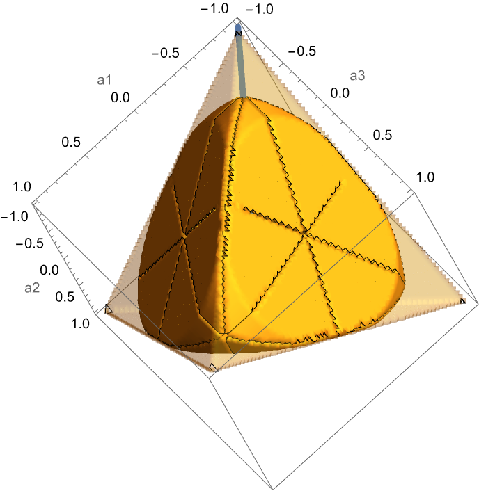
Figure 1: Semitransparent tetrahedron: set of Bell-diagonal states. The set is parameterized by the matrix elements $(a_{1},a_{2},a_{3})$ in Eq. (40). Solid figure inside the tetrahedron: set of local states. Solid grey line: set of Werner states.

Collecting the above results, for any Bell-diagonal state it is rather straightforward to derive the following formula relating the coefficients $\vec{a}=(1,a_{1},a_{2},a_{3})^{T}$ of the matrix $\alpha$ and the eigenvalues $\vec{e}=(e_{1},...,e_{4})^{T}$ of the density matrix:

$$\begin{bmatrix}1\\ a_{1}\\ a_{2}\\ a_{3}\end{bmatrix}=\begin{bmatrix}1&1&1&1\\ 1&1&-1&-1\\ 1&-1&1&-1\\ -1&1&1&-1\end{bmatrix}\begin{bmatrix}e_{1}\\ e_{2}\\ e_{3}\\ e_{4}\end{bmatrix}\,.$$ (41)

The matrix in the above expression is unitary upon multiplication by $1/2$. It follows that

$$\begin{bmatrix}e_{1}\\ e_{2}\\ e_{3}\\ e_{4}\end{bmatrix}=\frac{1}{4}\begin{bmatrix}1&1&1&-1\\ 1&1&-1&1\\ 1&-1&1&1\\ 1&-1&-1&-1\end{bmatrix}\begin{bmatrix}1\\ a_{1}\\ a_{2}\\ a_{3}\end{bmatrix}\,,$$ (42)

so that positivity and normalization of the sum of the eigenvalues allow to represent the set of all Bell-diagonal states parameterized by the three-dimensional vector $(a_{1},a_{2},a_{3})$ as shown in Fig. (1).

VI.2 Werner states

A particular subclass of the Bell-diagonal states are the Werner states $\rho_{w}$, described by one free parameter $|a_{1}|=|a_{2}|=|a_{3}|\equiv w$. Formally, a Werner state is a convex combination of the maximally mixed state with any one of the four Bell states. This class of states, first introduced by R. F. Werner Werner1989 , is important as it provides the paramount example of a set of states that for $\frac{1}{3}\leq w\leq\frac{1}{\sqrt{2}}$ are entangled but nevertheless local.

VI.3 Properties of local states

Let $(d_{1},d_{2},d_{3})$ be the singular values in the decomposition Eq. (35) and, without loss of generality let $d_{1}\geq d_{2}\geq d_{3}$. As proved in Ref. Horodecki1995 , a state is local if and only if

$$d_{1}^{2}+d_{2}^{2}\leq 1.$$ (43)

We prove the following:

Lemma 1. If $\rho$ is a local state with given $(\alpha_{0i},\alpha_{i0},A)$ then $\rho^{-}$ given by $(-\alpha_{0i},-\alpha_{i0},A)$ is also a local state.
Proof. It suffices to consider a local transformation that for $i=1,2,3$ changes $\sigma_{i}$ into $-\sigma_{i}$.

Lemma 2. For any local state $\rho$ with given $(\alpha_{0i},\alpha_{i0},A)$ there exists a local state $\rho^{\prime}$ with the same $A$ but $\alpha_{0i}=\alpha_{i0}=0$
Proof. Consider the convex combination

$$\rho^{\prime}=\frac{1}{2}\rho+\frac{1}{2}\rho^{-}.$$ (44)

Indeed, for such a combination we have

$$\alpha=\begin{bmatrix}\alpha_{00}&0\\ 0&A\end{bmatrix}.$$ (45)

Now, convex combinations of local states are local: by virtue of the property of shared randomness, if there exists a hidden variable model for each of the states in the combination, then there must exist a hidden variable model for their classical statistical mixture.

VI.4 Properties of symmetric states

Proposition 1. For any jointly convex and unitarily invariant functional $D$ of pairs of two-qubit density matrices

$$\min_{\rho^{loc}\in\sigma}D(\rho_{w},\rho^{loc})=\min_{\rho^{loc}_{w}\in\sigma}D(\rho_{w},\rho^{loc}_{w})\,,$$ (46)

where $\rho_{w}$ is a Werner state, $\rho^{loc}$ is a local state, and $\rho^{loc}_{w}$ is a local Werner state.

Proof. The proof is based on the following observations:

• Obs. 1. Invariance of Werner states under the same local unitary transformations on both subsystems:

  $$\forall\ {\rm unitary}\ U:\qquad\left(U\otimes U\right)\rho_{w}\left(U^{\dagger}\otimes U^{\dagger}\right)=\rho_{w}.$$ (47)

• Obs. 2. Local unitary transformations are resource non-generating (RNG) for nonlocality; in particular, $\left(U\otimes U\right)\rho^{loc}\left(U^{\dagger}\otimes U^{\dagger}\right)$ remains local.

• Obs. 3. Any convex combination of local states is a local state.

• Obs. 4. Twirling always projects on Werner states. Therefore, we have that for any given class of density matrices $\rho^{a}$

  $$\int dU\ \left(U\otimes U\right)\rho^{a}\left(U^{\dagger}\otimes U^{\dagger}\right)=\rho^{a}_{w}\,,$$ (48)

  where the integral is taken over the Haar measure on the set of unitary transformations.

From the unitary invariance of $D$ we have

$$D(\rho_{w},\rho^{loc}) = D\left(U\otimes U\rho_{w}U^{\dagger}\otimes U^{\dagger}\,,\,U\otimes U\rho^{loc}U^{\dagger}\otimes U^{\dagger}\right)$$ (49)

$$= \int dU\ D(U\otimes U\rho_{w}U^{\dagger}\otimes U^{\dagger}\,,\,U\otimes U\rho^{loc}U^{\dagger}\otimes U^{\dagger})$$ (50)

$$\geq D\bigg{(}\int dU\ U\otimes U\rho_{w}U^{\dagger}\otimes U^{\dagger}\,,\,\int dU\ U\otimes U\rho^{loc}U^{\dagger}\otimes U^{\dagger}\bigg{)}$$ (51)

$$= D(\rho_{w},\rho^{loc}_{w})\,.$$ (52)

Here the first and second lines come from unitary invariance of $D$; the third follows from the joint convexity; and the fourth from Obs. 1 - 4 above.

Similar propositions hold for general Bell-diagonal states; however, in the general case the proof holds for fairly smaller symmetry classes.

Proposition 2. For any jointly convex and unitarily invariant functional $D$ of pairs of two-qubit density matrices, the closest local state to a Bell-diagonal state is Bell-diagonal:

$$\min_{\rho_{loc}\in\sigma}f(\rho_{BD},\rho_{loc})=\min_{\rho_{BD,loc}\in\sigma}f(\rho_{BD},\rho_{BD,loc})\,,$$ (53)

where $\rho_{BD}$ denotes a Bell-diagonal state, $\rho_{loc}$ a local state, and $\rho_{BD,loc}$ a local Bell-diagonal state.

Proof. The symmetry class that we consider contains the simultaneous local $\pi$-rotations of qubits around the three Pauli axes. Rotation $R_{1}$ around $\sigma_{1}$ changes $\sigma_{2}$ and $\sigma_{3}$ to $-\sigma_{2}$ and $-\sigma_{3}$ respectively. Rotations $R_{2}$ and $R_{3}$ operate analogously. These transformations are local and unitary, therefore they cannot change the locality of a quantum state. Moreover, these transformations preserve Bell-diagonal states. Indeed, let us consider the general state representation Eq. (31). Under rotation $R_{1}$ we have the following transformation:

$$\alpha=\begin{pmatrix}1&a_{01}&a_{02}&a_{03}\\ a_{10}&a_{11}&a_{12}&a_{13}\\ a_{20}&a_{21}&a_{22}&a_{23}\\ a_{30}&a_{31}&a_{32}&a_{33}\end{pmatrix}\,\,\longrightarrow\,\,\alpha_{1}=\begin{pmatrix}1&a_{01}&-a_{02}&-a_{03}\\ a_{10}&a_{11}&-a_{12}&-a_{13}\\ -a_{20}&-a_{21}&a_{22}&a_{23}\\ -a_{30}&-a_{31}&a_{32}&a_{33}\end{pmatrix}.$$ (54)

The average $\rho^{\prime}=1/2(\rho+R_{1}(\rho))$ enjoys the representation

$$\alpha_{1}^{\prime}=\begin{pmatrix}1&a_{01}&0&0\\ a_{10}&a_{11}&0&0\\ 0&0&a_{22}&a_{23}\\ 0&0&a_{32}&a_{33}\end{pmatrix}.$$ (55)

Applying rotation $R_{2}$ to $\rho^{\prime}$ and averaging the result with $\rho^{\prime}$ leads to the state with diagonal representation Eq. (39), i.e. a Bell-diagonal state. The total transformation that projects a given state to a Bell-diagonal state takes the compact form

$$\rho\,\,\longrightarrow\,\,\frac{1}{2}\left(\frac{1}{2}(\rho+R_{1}(\rho))+R_{2}\left(\frac{1}{2}(\rho+R_{1}(\rho))\right)\right).$$ (56)

This transformation obviously preserves the Bell-diagonal states, does not change the locality, and is a composition of joint local unitaries and averaging. The proof of Proposition 2 is thus immediately completed by straightforwardly adapting the reasoning followed in the proof of Proposition 1.

VII Bell nonlocality of two-qubit states

Exploiting the results derived in the previous section, we can proceed to quantify the Bell nonlocality of two-qubit states using the Hilbert space based distance and relative entropy measures with respect to the set of local two-qubit states. Explicit examples will include Werner states, Bell-diagonal states, and reduced convex combinations of Bell states. These important classes of states are routinely considered in the study of quantum resource theories, starting from the pioneering investigations on entanglement and discord Wootters1997 ; Wootters1998 ; Henderson_Vedral2001 .

VII.1 Werner states

VII.1.1 Hilbert-Schmidt distance

Consider the squared Hilbert-Schmidt (HS) distance defined on a generic pair $\{\rho_{1},\rho_{2}\}$ of two-qubit states as induced by the HS norm Eq. (16). Using Eq. (31) and the properties of the Pauli matrices:

$$\|\rho_{1}-\rho_{2}\|_{HS}\,=\,\|\alpha_{1}-\alpha_{2}\|_{HS}\,.$$ (57)

It follows from Proposition 1, Eq. (46), that the closest local state to a Werner state is also a Werner state with $w\leq 1/\sqrt{2}$. Hence, for nonlocal Werner states, i.e. with $w\geq 1/\sqrt{2}$ :

$$\mathcal{M}_{HS}(\rho_{w})=\min_{\rho^{loc}_{w}\in\sigma}\left\|\rho_{w}-\rho^{loc}\right\|_{HS}^{2}=\left\|\frac{1}{\sqrt{2}}\mathbf{1}-w\mathbf{1}\right\|_{HS}^{2}=3\left(\frac{1}{\sqrt{2}}-w\right)^{2}\,,$$ (58)

where $\mathbf{1}$ is the identity matrix and $w\in\left(1/\sqrt{2},1\right]$. Correctly, the maximum is achieved by the maximally entangled Bell states corresponding to $w=1$ :

$$\mathcal{M}_{HS}^{max}\,=\,\frac{3}{2}\left(3-2\sqrt{2}\right)\,.$$ (59)

The behavior of the normalized HS geometric measure of nonlocality for Werner states $\widetilde{\mathcal{M}}_{HS}=\mathcal{M}_{HS}(\rho_{w})/\mathcal{M}_{HS}^{max}$ as a function of the $w$ parameter is reported in Fig. 2. The plot is a parabola, as the the HS distance is simply the Euclidean distance in the three-dimensional space of Fig. 1.

VII.1.2 Hellinger distance

Recalling again the consequences of Proposition 1, Eq. (46), the measure of Bell nonlocality for Werner states based on the (squared) Hellinger distance, Eq. (19), reads

$$\mathcal{M}_{He}(\rho_{w})=\min_{\rho_{w}^{loc}\in\sigma}D^{2}_{He}(\rho_{w},\rho_{w}^{loc})=2-\frac{1}{2}\left(3\sqrt{(1-w)\left(1-\frac{1}{\sqrt{2}}\right)}+\sqrt{(1+3w)\left(1+\frac{3}{\sqrt{2}}\right)}\right)\,,$$ (60)

where $w\in(1/\sqrt{2},1]$. Here we have used the relation between the eigenvalues of the state density matrix and the Werner parameter $w$ which is derived directly from Eq. (42). As $|a_{1}|=|a_{2}|+|a_{3}|=w$, the signs of the matrix elements $a_{i}$ identify the states corresponding to different corners of the state tetrahedron in Fig. 1. The Hellinger measure is maximized by the Bell states at $w=1$ :

$$\mathcal{M}_{He}^{max}=2-\sqrt{1+\frac{3}{\sqrt{2}}}\,\,.$$ (61)

The behavior of the normalized Hellinger geometric measure of Bell nonlocality for Werner states $\widetilde{\mathcal{M}}_{He}=\mathcal{M}_{He}(\rho_{w})/\mathcal{M}_{He}^{max}$ as a function of the $w$ parameter is shown in Fig. 2.

VII.1.3 Bures distance

In the case of commuting operators the Bures distance and the Hellinger distance coincide. This is indeed the case for Werner density matrices. Therefore, the Bures and Hellinger measures of nonlocality coincide on Werner states $\rho_{w}$:

$$\mathcal{M}_{Bu}(\rho_{w})=\mathcal{M}_{He}(\rho_{w})\,.$$ (62)

VII.1.4 Trace distance

The geometric measure of Bell nonlocality of Werner states based on the trace distance Eq. (24) reads:

$$\mathcal{M}_{Tr}(\rho_{w})=\min_{\rho_{w}^{loc}\in\sigma}D_{Tr}(\rho_{w},\rho_{w}^{loc})=\frac{3}{2}\left|w-\frac{1}{\sqrt{2}}\right|=\frac{3}{2}\left(w-\frac{1}{\sqrt{2}}\right)\,,$$ (63)

where the last equality follows from the fact that without loss of generality we can limit the analysis to the interval $w\in(1/\sqrt{2},1]$. The maximum value is achieved at $w=1$ by the Bell states:

$$\mathcal{M}_{Tr}^{max}=\frac{3}{2}\left(1-\frac{1}{\sqrt{2}}\right)\,.$$ (64)

The normalized trace measure of nonlocality for Werner states $\widetilde{\mathcal{M}}_{Tr}=\mathcal{M}_{Tr}(\rho_{w})/\mathcal{M}_{Tr}^{max}$ as a function of the $w$ parameter is shown in figure 2.

VII.1.5 Relative entropy

It is straightforward to verify that for a nonlocal Werner state in the interval $w\geq 1/\sqrt{2}\,$ its relative entropy Eq. (7) with respect to the set $\sigma$ of local states is minimized by the local state with $w=1/\sqrt{2}$ , so that:

$$\mathcal{M}_{Re}(\rho_{w})=\min_{\rho_{w}^{loc}\in\sigma}S(\rho_{w}|\rho_{w}^{loc}) = \frac{3(1-w)}{4}\log_{2}\left(\frac{3(1-w)}{4}\right)+\frac{1+3w}{4}\log_{2}\left(\frac{1+3w}{4}\right)+$$ (65)

$$- \frac{3(1-w)}{4}\log_{2}\left(\frac{\sqrt{2}-1}{4\sqrt{2}}\right)-\frac{1+3w}{4}\log_{2}\left(\frac{\sqrt{2}+3}{4\sqrt{2}}\right)\,.$$

The maximum value achieved by the Bell states at $w=1$ reads

$$\mathcal{M}_{Re}^{max}=2-\log_{2}{\bigg{(}1+\frac{3}{\sqrt{2}}\bigg{)}}\,.$$ (66)

The normalized relative entropy measure of Bell nonlocality for Werner states $\widetilde{\mathcal{M}}_{Re}=\mathcal{M}_{Re}(\rho_{w})/\mathcal{M}_{Re}^{max}$ as a function of the $w$ parameter is reported in Fig. 2.

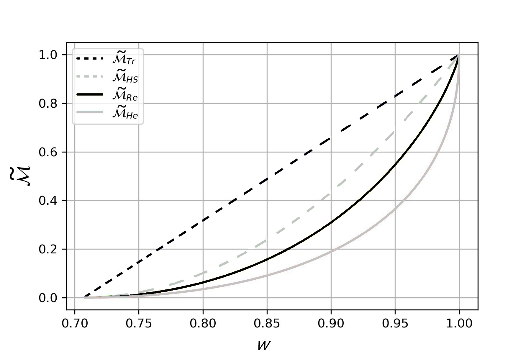
Figure 2: Normalized geometric measures of nonlocality for Werner states as a function of the Werner parameter $w$ in the interval $\frac{1}{\sqrt{2}}\leq w\leq 1$. Black dashed straight line: Trace measure $\widetilde{\mathcal{M}}_{Tr}$. Grey dashed curve: Hilbert-Schmidt measure $\widetilde{\mathcal{M}}_{HS}$. Black solid curve: Relative entropy measure $\widetilde{\mathcal{M}}_{Re}$. Grey solid curve: Hellinger measure $\widetilde{\mathcal{M}}_{He}$. All plotted quantities are dimensionless.

VII.2 Bell-diagonal states

VII.2.1 Hilbert-Schmidt distance

All Bell-diagonal states can be represented as points in a tetrahedron, as shown in Fig. 1, with vertices representing Bell states. The points are given by three dimensional vectors $\vec{\alpha}$ that appear in Eq. (57). This equation implies that the Euclidean distance in the space represented in Fig. 1 coincides with the HS distance in the space of density matrices of Bell-diagonal states. Moreover, for all Bell-diagonal states the closest local state is a Bell-diagonal state, as proved in Proposition 2, Eq. (53). The set of local states is represented by points in the solid figure inscribed inside the tetrahedron, see Fig. 1. Hence, the Euclidean distance between the points representing nonlocal Bell-diagonal states and the boundary of the solid figure yields the HS-based geometric measure of nonlocality. Exploiting the Horodecki locality criterion Eq. (43), the separation surface between local and nonlocal Bell-diagonal state is identified by the solutions of the equation

$$\max_{i,ji\neq j}\{a_{i}^{2}+a_{j}^{2}\}=1\,.$$ (67)

Combining the above with Proposition 2, Eq. (53), the minimum of the squared HS distance is determined as

$$\min_{\rho_{BD}^{loc}\in\sigma}\left\|\rho_{BD}-\rho_{BD}^{loc}\right\|_{HS}^{2}=\min_{a_{i}^{loc}}\frac{1}{2}\displaystyle\sum_{i=1}^{3}(a_{i}-a_{i}^{loc})^{2}\,,$$ (68)

with the provision that the states $\rho_{BD}$ belong to the surface Eq. (67).

Considering first the case $|a_{1}^{loc}|,|a_{2}^{loc}|>|a_{3}^{loc}|$, we can proceed to determine the minimum by introducing a Lagrange multiplier $\lambda$. The associated Lagrange variational function reads

$$\Gamma(a_{1}^{loc},a_{2}^{loc},a_{3}^{loc},\lambda)\equiv\displaystyle\sum_{i=1}^{3}(a_{i}-a_{i}^{loc})^{2}+\lambda[(a_{1}^{loc})^{2}+(a_{2}^{loc})^{2}-1]\,.$$ (69)

Vanishing of the gradient of $\Gamma$ leads to

$\begin{cases}(a_{1}-a_{1}^{loc})+\lambda a_{1}^{loc}=0,\\ (a_{2}-a_{2}^{loc})+\lambda a_{2}^{loc}=0,\\ (a_{3}-a_{3}^{loc})=0,\\ (a_{1}^{loc})^{2}+(a_{2}^{loc})^{2}-1=0.\end{cases}$

Denoting the minima by $\tilde{a}_{i}^{loc}$, the solution reads

$$\tilde{a}_{1}^{loc}=\frac{-a_{2}\pm\sqrt{a_{2}^{2}+4}}{2},$$

$$\tilde{a}_{2}^{loc}=\frac{-a_{1}\pm\sqrt{a_{1}^{2}+4}}{2},$$

$$\tilde{a}_{3}^{loc}=a_{3}.$$ (70)

By Eq. (68) the (un-normalized) HS geometric measure of nonlocality for Bell-diagonal states is thus

$$\mathcal{M}_{HS}(\rho_{BD})=\frac{1}{4}\left[(a_{1}-a_{2})^{2}+\frac{a_{1}^{2}+a_{2}^{2}}{2}+(a_{2}-a_{1})\bigg{(}\sqrt{a_{1}^{2}+4}-\sqrt{a_{2}^{2}+4}\bigg{)}+2\right].$$ (71)

The remaining cases $|a_{2}^{loc}|,|a_{3}^{loc}|>|a_{1}^{loc}|$ and $|a_{1}^{loc}|,|a_{3}^{loc}|>|a_{2}^{loc}|$ can be immediately found by symmetry and the global minimum is determined over all possible cases. For the maximally nonlocal Bell states the minimum is attained when $|a_{1}^{loc}|=|a_{2}^{loc}|=|a_{3}^{loc}|\equiv w^{2}$, with $w$ the Werner parameter. The constraints in Eq. (69) thus reduce to $2w^{2}=1$, i.e. $w=1/\sqrt{2}$, and $\mathcal{M}_{HS}$ achieves its maximum $\mathcal{M}_{HS}^{max}$, Eq. (59). Using Eqs. (41) and (42) the transformation from the matrix elements $\{a_{i}\}$ to the eigenvalues $\{e_{i}\}$ of the density matrix follows immediately. The behavior of the normalized HS measure of Bell nonlocality $\widetilde{\mathcal{M}}_{HS}=\mathcal{M}_{HS}/\mathcal{M}_{HS}^{max}$ for Bell-diagonal states as a function of the eigenvalues $e_{1}$, $e_{2}$ in the case of $e_{4}=0$ is reported in Fig. 3.

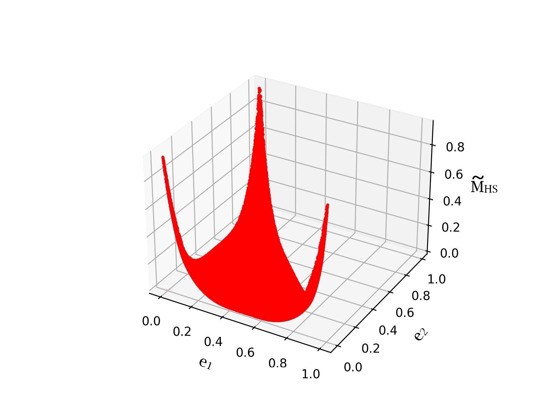
Figure 3: Normalized Hilbert-Schmidt measure $\widetilde{\mathcal{M}}_{HS}$ of Bell nonlocality for Bell-diagonal states as a function of the two free parameters $e_{1}$ and $e_{2}$, with $e_{4}=0$, $e_{3}=1-e_{1}-e_{2}$, and normalization coefficient $\mathcal{M}_{HS}^{max}$. The maximum $\widetilde{\mathcal{M}}_{HS}=1$ is reached in the three cases $(e_{1},e_{2},e_{3})=(1,0,0)$; $(e_{1},e_{2},e_{3})=(0,1,0)$; and $(e_{1},e_{2},e_{3})=(0,0,1)$. Each case corresponds to a different Bell state. The central region of minima is composed by local states, i.e. states with $\widetilde{\mathcal{M}}_{HS}=0$. All plotted quantities are dimensionless.

VII.2.2 Hellinger distance

Each of the eigenvalues $\{e_{i}^{k}\}$ of a density matrix $\rho_{k}$ is the probability that a system in state $\rho_{k}$ collapses in the eigenstate relative to that eigenvalue. For a Bell-diagonal state $\rho_{BD}$ the eigenstates are obviously the four Bell states. Recalling Proposition 2, Eq. (53), and Eq. (19) the minimization process on the Hellinger distance squared yields the Hellinger geometric measure of Bell nonlocality $\mathcal{M}_{He}(\rho_{BD})$ for Bell-diagonal states:

$$\mathcal{M}_{He}(\rho_{BD})=\min_{\rho_{BD}^{loc}\in\sigma}D^{2}_{He}(\rho_{BD},\rho_{BD}^{loc})=\min_{\rho^{loc}\in\sigma}\left\{\displaystyle\sum_{i=1}^{4}\bigg{(}\sqrt{e_{i}}-\sqrt{e_{i}^{loc}}\bigg{)}^{2}\right\}\,.$$ (72)

Using Eq.(42) we can rewrite the condition Eq. (67) in terms of the eigenvalues $\{e_{i}^{loc}\}$. Fixing, for instance, the case $|a_{1}|,|a_{2}|>|a_{3}|$, one has:

$$(e_{1}-e_{3})^{2}+(e_{2}-e_{4})^{2}\,>\,\frac{1}{2}\,.$$ (73)

For probabilities, their positivity $e_{i}>0$ and normalization condition $\displaystyle\sum_{i}e_{i}=1$ define a clove of a unitary $4-$sphere in the $\sqrt{e_{i}}-$space. Therefore, the set of nonlocal states with $|a_{1}|,|a_{2}|>|a_{3}|$ is represented in the $\sqrt{e_{i}}-$space by the intersection of the hypervolume Eq. (73) with the unitary semi-sphere centered in the origin. Since the distance in this space is the Euclidean one, the minimum in Eq. (72) in the case $|a_{1}^{loc}|,|a_{2}^{loc}|>|a_{3}^{loc}|$ is determined by imposing the constraint

$$(e_{1}^{loc}-e_{3}^{loc})^{2}+(e_{2}^{loc}-e_{4}^{loc})^{2}=\frac{1}{2}\,.$$ (74)

Recalling Eq. (19), the above relation identifying the region of separation between local and nonlocal state is obtained when $\sum_{i=1}^{4}\sqrt{e_{i}e_{i}^{loc}}$ is maximum. We can thus proceed by the method of Lagrange multipliers and introduce the following Lagrangian function

$$\Gamma(e_{i}^{loc},\lambda_{1},\lambda_{2})\equiv\displaystyle\sum_{i=1}^{4}\sqrt{e_{i}e_{i}^{loc}}+\lambda_{1}\bigg{[}(e_{1}^{loc}-e_{3}^{loc})^{2}+(e_{2}^{loc}-e_{4}^{loc})^{2}-\frac{1}{2}\bigg{]}+\lambda_{2}\left(\displaystyle\sum_{i=1}^{4}e_{i}^{loc}-1\right)\,.$$ (75)

Taking the gradient of $\Gamma$ and imposing its vanishing yields

$\begin{cases}\frac{1}{2}\sqrt{\frac{e_{1}}{e_{1}^{loc}}}+2\lambda_{1}(e_{1}^{loc}-e_{3}^{loc})+\lambda_{2}=0\\ \vspace{0.2cm}\par\frac{1}{2}\sqrt{\frac{e_{2}}{e_{2}^{loc}}}+2\lambda_{1}(e_{2}^{loc}-p_{4}^{loc})+\lambda_{2}=0,\\ \vspace{0.2cm}\par\frac{1}{2}\sqrt{\frac{e_{3}}{e_{3}^{loc}}}-2\lambda_{1}(e_{1}^{loc}-e_{3}^{loc})+\lambda_{2}=0,\\ \vspace{0.2cm}\par\par\frac{1}{2}\sqrt{\frac{e_{4}}{e_{4}^{loc}}}-2\lambda_{1}(e_{2}^{loc}-e_{4}^{loc})+\lambda_{2}=0,\\ \vspace{0.2cm}\par\par e_{1}^{loc}+e_{2}^{loc}+e_{3}^{loc}+e_{4}^{loc}=1,\\ \vspace{0.2cm}\par\par(e_{1}^{loc}-e_{3}^{loc})^{2}+(e_{2}^{loc}-e_{4}^{loc})^{2}=\frac{1}{2}\,.\end{cases}$

From the above relations one immediately determines the Lagrange multipliers:

$$\lambda_{1}=-\frac{\sqrt{\frac{e_{1}}{e_{1}^{loc}}}-\sqrt{\frac{e_{3}}{e_{3}^{loc}}}}{8(e_{1}^{loc}-e_{3}^{loc})}=-\frac{\sqrt{\frac{e_{2}}{e_{2}^{loc}}}-\sqrt{\frac{e_{4}}{e_{4}^{loc}}}}{8(e_{2}^{loc}-e_{4}^{loc})}\,,$$ (76)

$$\lambda_{2}=-\frac{1}{4}\bigg{(}\sqrt{\frac{e_{1}}{e_{1}^{loc}}}+\sqrt{\frac{e_{3}}{e_{3}^{loc}}}\bigg{)}=-\frac{1}{4}\bigg{(}\sqrt{\frac{e_{2}}{e_{2}^{loc}}}+\sqrt{\frac{e_{4}}{e_{4}^{loc}}}\bigg{)}\,,$$ (77)

so that

$\begin{cases}\sqrt{\frac{e_{1}}{e_{1}^{loc}}}+\sqrt{\frac{e_{3}}{e_{3}^{loc}}}=\sqrt{\frac{e_{2}}{e_{2}^{loc}}}+\sqrt{\frac{e_{4}}{e_{4}^{loc}}}\,,\\ \vspace{0.2cm}\par\par\bigg{(}\sqrt{\frac{e_{1}}{e_{1}^{loc}}}-\sqrt{\frac{e_{3}}{e_{3}^{loc}}}\bigg{)}(e_{2}^{loc}-e_{4}^{loc})=\bigg{(}\sqrt{\frac{e_{2}}{e_{2}^{loc}}}-\sqrt{\frac{e_{4}}{e_{4}^{loc}}}\bigg{)}(e_{1}^{loc}-e_{3}^{loc})\,,\\ \vspace{0.2cm}\par\par e_{1}^{loc}+e_{2}^{loc}+e_{3}^{loc}+e_{4}^{loc}=1\,,\\ \vspace{0.2cm}\par\par(e_{1}^{loc}-e_{3}^{loc})^{2}+(e_{2}^{loc}-e_{4}^{loc})^{2}=\frac{1}{2}\,.\end{cases}$

The remaining cases can be treated symmetrically; the absolute minimum is determined by the smallest value with respect to all the possible cases. In the case of Bell states, e.g. $e_{1}=1$, $e_{2}=e_{3}=e_{4}=0$, it is straightforward to verify that the minimum is reached for $e_{1}^{loc}=\frac{1+3t}{4}$, $e_{2}^{loc}=e_{3}^{loc}=e_{4}^{loc}=\frac{1-t}{4}$ , with $t=\frac{1}{\sqrt{2}}$. Therefore, as it must be, we find that the maximum value $\mathcal{M}_{He}^{max}$ of the Hellinger geometric measure of Bell nonlocality Eq. (72) coincides with that of the Hellinger measure for Werner states, Eq. (60), with Werner parameter $w=1$.

On the other hand, we see that the above minimization procedure cannot always yield a closed formula of the Hellinger measure of Bell nonlocality for generic Bell-diagonal states. This is implied by the type of bound on the set of local states and the form of the function one needs to minimize. Indeed, the above algebraic systems yields that in order to find the minimum one must determine the roots of a polynomial of the fifth order. Therefore, from the Abel-Ruffini-Seralian theorem it follows that it is impossible to obtain a closed analytical formula by quadratures for the roots in terms of the coefficients of the polynomial. Of course, the solutions can be determined to any desired degree of precision by standard approximation procedures such as, e.g., the Newton-Raphson method or the Laguerre iterative scheme. Alternatively, we can proceed analytically in special but relevant instances, such as the Bell states or, as we will show later on, the Bell-diagonal states with one free parameter.

VII.2.3 Bures distance

In analogy with the case of Werner states, also in the case of Bell-diagonal states the density operators commute and the Bures and Hellinger distances coincide, so that

$$\mathcal{M}_{Bu}(\rho_{BD})=\mathcal{M}_{He}(\rho_{BD})\,.$$ (78)

VII.2.4 Relative entropy

In the case of the relative entropy we assume that in order to determine the minimum in Eq. (7) we can continue to impose the constraint Eq. (74). In other words, we expect that also for the relative entropy of nonlocality of Bell-diagonal states the closest local state belongs to the same surface as for the Hellinger and Bures measures. Assuming the above hypothesis, the minimum in Eq. (7) is realized when

$$\sum_{i=1}^{3}e_{i}\log_{2}{e_{i}^{loc}}$$ (79)

achieves its maximum.
Fixing as usual, to begin with, the case $|a_{1}|,|a_{2}|>|a_{3}|$, the Lagrange function associated to the Lagrange multipliers takes the form

$$\Gamma(e_{i}^{loc},\lambda_{1},\lambda_{2})\equiv\displaystyle\sum_{i=1}^{4}e_{i}\log_{2}{e_{i}^{loc}}+\lambda_{1}[(e_{1}^{loc}-e_{3}^{loc})^{2}+(e_{2}^{loc}-e_{4}^{loc})^{2}-\frac{1}{2}]+\lambda_{2}\left(\displaystyle\sum_{i=1}^{4}e_{ij}^{loc}-1\right)\,,$$ (80)

which leads to

$\begin{cases}\frac{e_{1}}{e_{1}^{loc}\ln{2}}+2\lambda_{1}(e_{1}^{loc}-e_{3}^{loc})+\lambda_{2}=0,\\ \vspace{0.2cm}\par\frac{p_{01}}{e_{2}^{loc}\ln{2}}+2\lambda_{1}(e_{2}^{loc}-e_{4}^{loc})+\lambda_{2}=0,\\ \vspace{0.2cm}\par\frac{e_{3}}{e_{3}^{loc}\ln{2}}-2\lambda_{1}(e_{1}^{loc}-e_{3}^{loc})+\lambda_{2}=0,\\ \vspace{0.2cm}\par\frac{e_{4}}{e_{4}^{loc}\ln{2}}-2\lambda_{1}(e_{2}^{loc}-e_{4}^{loc})+\lambda_{2}=0,\\ \vspace{0.2cm}\par e_{1}^{loc}+e_{2}^{loc}+e_{3}^{loc}+e_{4}^{loc}=1,\\ \vspace{0.2cm}\par(e_{1}^{loc}-e_{2}^{loc})^{2}+(e_{3}^{loc}-e_{4}^{loc})^{2}=\frac{1}{2}.\end{cases}$

It is straightforward to show that the above relations reduce to

$\begin{cases}\frac{e_{1}}{e_{1}^{loc}}+\frac{e_{3}}{e_{3}^{loc}}=\frac{e_{2}}{e_{2}^{loc}}+\frac{e_{4}}{e_{4}^{loc}},\\ \vspace{0.2cm}\par\bigg{(}\frac{e_{3}}{e_{3}^{loc}}-\frac{e_{1}}{e_{1}^{loc}}\bigg{)}(e_{2}^{loc}-e_{4}^{loc})=\bigg{(}\frac{e_{4}}{e_{4}^{loc}}-\frac{e_{2}}{e_{2}^{loc}}\bigg{)}(e_{1}^{loc}-e_{3}^{loc}),\\ \vspace{0.2cm}\par e_{1}^{loc}+e_{2}^{loc}+e_{3}^{loc}+e_{4}^{loc}=1,\\ \vspace{0.2cm}\par(e_{1}^{loc}-e_{2}^{loc})^{2}+(e_{3}^{loc}-e_{4}^{loc})^{2}=\frac{1}{2}.\par\end{cases}$

In analogy with the case of the Hellinger measure, the above algebraic system is of higher order and not amenable to a solution by elementary quadratures. Therefore, in the following subsection we will consider the particular instance of one-parameter Bell-diagonal states that allows for the full analytical evaluation of the entire set of geometric and entropic measures of Bell nonlocality.

VII.3 Bell-diagonal states with one free parameter

Let us consider Bell-diagonal states that are convex combinations of only two of the four Bell states. For instance, let us choose $e_{2}=e_{4}=0$ , $e_{1}=p$ , and $e_{3}=1-p$ , with $p$ free parameter in the interval $[0,1]$. Such Bell-diagonal states represent all possible convex combinations of the first and third Bell states of Eq. (37). Moving to symplectic space and recalling Eqs. (42), this instance corresponds to $a_{1}=a$, $a_{2}=-a$, and $a_{3}=1$, with $a=2p-1$.

For this class of states the locality condition Eq. (43) is fulfilled only for $p=\frac{1}{2}$; therefore, such states are nonlocal for $0\leq p\leq 1$, with the exception of $p=\frac{1}{2}$. The behavior of the four normalized measures of Bell nonlocality as functions of the convex combination parameter $p$ in the half-interval $p\geq\frac{1}{2}$ is reported in Fig. 4. We see that all measures vanish at $p=\frac{1}{2}$ and reach their maximum at $p=1$, i.e. on the first Bell state. For all measures, the normalization coefficients turn out to be the same as the ones of the nonlocality measures for Werner states, in agreement with Proposition 1, Eq. (46), and Proposition 2, Eq. (53). The case $p\leq\frac{1}{2}$ is readily obtained by symmetry.

It is straightforward to verify that the above-described behavior is generic, i.e. it does not depend on the pair of Bell states that are chosen as entries of the convex combination.

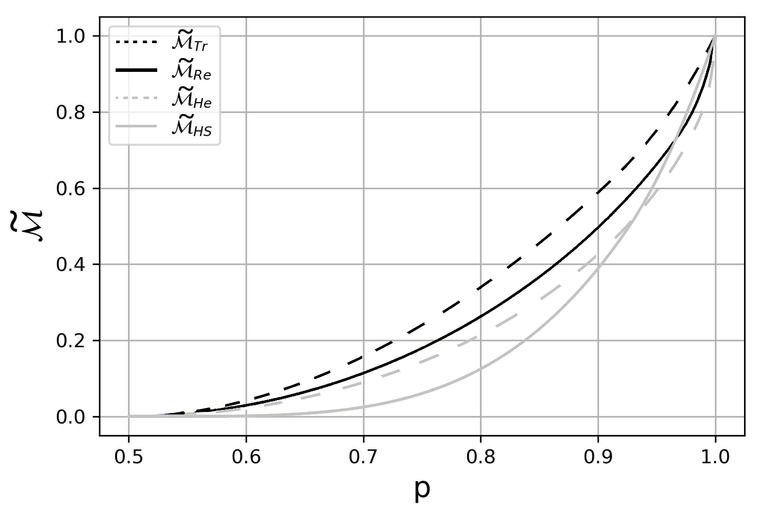
Figure 4: Normalized measures of Bell nonlocality for the convex combination of two Bell states as functions of the convex combination parameter $p$ in the interval $p\geq\frac{1}{2}$. The same behavior holds in the symmetric case $p\leq\frac{1}{2}$, with the maximum achieved in $p=0$. Black dashed curve: Trace measure $\widetilde{\mathcal{M}}_{Tr}$. Black solid curve: Relative entropy measure $\widetilde{\mathcal{M}}_{Re}$. Grey dashed curve: Hellinger measure $\widetilde{\mathcal{M}}_{He}$. Grey solid curve: Hilbert-Schmidt measure $\widetilde{\mathcal{M}}_{HS}$. All plotted quantities are dimensionless.

VIII Discussion and outlook

We have developed a general resource theory of Bell nonlocality whose defining elements are the state vectors in Hilbert space. We have identified the basic traits of such a theory, including the set of local states and the free operations, and we have discussed the concept of maximally nonlocal state. The qualification of Bell nonlocality that we have adopted is based on the concept of Local Operations and Shared Randomness (LOSR) that induces a broader perspective on quantum nonlocality and its relationship with entanglement theory, as advocated in Refs. Buscemi2012 ; Wolfe2020 ; Schmid2020b ; Rosset2020 ; Lipka2021 . The quantification of Bell nonlocality for quantum states in Hilbert space is naturally introduced in terms of geometric and entropic measures, in close methodological analogy with entanglement theory. Geometric measures define a structure and on ordering in the space of quantum states, and we have provided a detailed investigation of such structure for different classes of contractive distances (trace, Hellinger, Bures) in the case of two-qubit states by proving and exploiting the result that for contractive distances the closest local state to a Werner state is still a Werner state, and that an analogous result holds for Bell-diagonal states. We have confronted the ordering provided by contractive geometric measures of Bell nonlocality with the non-contractive Hilbert-Schmidt distance, and we have introduced the relative entropy of nonlocality as a further benchmark.

Generalizations and applications of the conceptual framework introduced in the present work are conceivable along different directions, such as the identification of the set of local states and the ordering of nonlocal states in finite-dimensional Hilbert spaces of dimension $D>2$, the extension to field-theoretical settings of elementary particle physics, and the use of the Hilbert space-based measures of Bell nonlocality as tools in the investigation and characterization of quantum collective phenomena and quantum phase transitions. Concerning the latter, a characterization of the ground states of quantum many-body systems in terms of Hilbert-space based measures of Bell nonlocality could provide novel and potentially profound insights on the degree of quantumness and quantumness hierarchies between different systems of quantum matter, in analogy with and complementing the very successful use of entanglement in condensed matter theory Laflorencie2016 ; Illuminati2022 .

The Hilbert-space characterization and quantification that we have introduced paves the way to the study of several important questions concerning quantum nonlocality. In entanglement theory, it is known that different entanglement measures can give rise to different orderings of quantum states; for instance, the entropy-based entanglement of formation and the entanglement negativity based on the PPT criterion induce a different ordering on the set of entangled Gaussian states Adesso2005 . Similar ordering issues might arise when determining the degree of Bell nonlocality of quantum states as quantified by the different geometric or entropic measures that we have introduced in the present work. A further important question concerns the characterization and quantification of extremal nonlocality in mixed states. In entanglement theory, maximally entangled mixed states are typically defined at fixed energy, or fixed degree of local and global entropies Adesso2003 ; Adesso2004 . An investigation along similar lined could lead to the identification of the maximally nonlocal mixed states at fixed global and/or local purities. In our opinion, a particularly challenging open problem whose eventual solution would bear far-reaching consequences revolves around the question whether the analogs of Werner states, i.e. mixed states that are local and yet entangled, exist in infinite-dimensional Hilbert spaces. In particular, it would be very interesting to determine the existence of Werner Gaussian states of two- and multimode continuous-variable systems, and to characterize their properties.

- (1) E. Chitambar and G. Gour, Quantum resource theories, Rev. Mod. Phys. 91, 025001 (2019).
- (2) T. A. Theurer, Resource theories of states and operations, Doctoral Dissertation, Universität Ulm (2021).
- (3) T. Theurer, N. Killoran, D. Egloff, and M. B. Plenio, Resource theory of superposition, Phys. Rev. Lett. 119, 230401 (2017).
- (4) R. Gallego and L. Aolita, Resource theory of steering, Phys. Rev. X 5, 041008 (2015).
- (5) R. Horodecki, P. Horodecki, M. Horodecki, and K. Horodecki, Quantum entanglement, Rev. Mod. Phys. 81, 865 (2009).
- (6) P. Contreras-Tejada, C. Palazuelos, and J. I. de Vicente, Resource theory of entanglement with a unique multipartite maximally entangled state, Phys. Rev. Lett. 122, 120503 (2019).
- (7) M. B. Plenio and S. Virmani, An introduction to entanglement measures, Quant. Inf. Comput. 7 1 , (2007).
- (8) Borivoje Dakić et al., Quantum discord as resource for remote state preparation, Nature Physics 8, 666 (2012).
- (9) Stefano Pirandola, Quantum discord as a resource for quantum cryptography, Scientific Reports 4, 6956 (2014).
- (10) A. Streltsov, G. Adesso, and M. B. Plenio, Quantum coherence as a resource, Rev. Mod. Phys. 89, 041003 (2017).
- (11) F. Buscemi, E. Chitambar, and W. Zhou, Complete resource theory of quantum incompatibility as quantum programmability, Phys. Rev. Lett. 124, 120401 (2020).
- (12) S. D. Bartlett, T. Rudolph, and R. W. Spekkens, Reference frames, superselection rules, and quantum information, Rev. Mod. Phys. 79, 555 (2007).
- (13) G. Gour and R. W. Spekkens, The resource theory of quantum reference frames: manipulations and monotones, New J. Phys. 10, 033023 (2008).
- (14) F. Buscemi, K. Kobayashi, and S. Minagawa, A complete and operational resource theory of measurement sharpness, Preprint arXiv:2303.07737 (2023).
- (15) F. G. S. L. Brandão, M. Horodecki, J. Oppenheim, J. M. Renes, and R. W. Spekkens, Resource theory of quantum states out of thermal equilibrium, Phys. Rev. Lett. 111, 250404 (2013).
- (16) G. Gour, M. P. Müller, V. Narasimhachar, R. W. Spekkens, and N. Y. Halpern, The resource theory of informational nonequilibrium in thermodynamics, Phys. Rep. 583, 1 (2015).
- (17) J. I. de Vicente, On nonlocality as a resource theory and nonlocality measures, J. Phys. A: Math. Theor. 47, 424017 (2014).
- (18) R. Gallego and L. Aolita, Nonlocality free wirings and the distinguishability between Bell boxes, Phys. Rev. A 95, 032118 (2017).
- (19) K. Kuroiwa and H. Yamasaki, General quantum resource theories: distillation, formation and consistent resource measures, Quantum 4, 355 (2020).
- (20) T. Gonda and R. W. Spekkens, Monotones in general resource theories, Compositionality 5, 7 (2023).
- (21) A. K. Ekert, Quantum cryptography based on Bell’s theorem, Phys. Rev. Lett. 67, 661 (1991).
- (22) C. H. Bennett, G. Brassard, C. Crépeau, R. Jozsa, A. Peres, and W. K. Wootters, Teleporting an unknown quantum state via dual classical and Einstein–Podolsky–Rosen channels, Phys. Rev. Lett. 70, 1895 (1993).
- (23) C. H. Bennett, P. W. Shor, J. A. Smolin, and A. V. Thapliyal, Entanglement-assisted classical capacity of noisy quantum channels, Phys. Rev. Lett. 83, 3081 (1999).
- (24) I. Devetak, A. W. Harrow, and A. Winter, A family of quantum protocols, Phys. Rev. Lett. 93, 230504 (2004).
- (25) K. Horodecki, M. Horodecki, P. Horodecki, and J. Oppenheim, Secure key from bound entanglement, Phys. Rev. Lett. 94, 160502 (2005).
- (26) I. Bengtsson and K. Życzkowski, Geometry of quantum states: an introduction to quantum entanglement (Cambridge University Press, Cambridge, 2017).
- (27) C. H. Bennett, G. Brassard, S. Popescu, B. Schumacher, J. A. Smolin, and W. K. Wootters, Purification of noisy entanglement and faithful teleportation via noisy channels, Phys. Rev. Lett. 76, 722 (1996).
- (28) C. H. Bennett, H. Bernstein, S. Popescu, and B. Schumacher, Concentrating partial entanglement by local operations, Phys. Rev. A 53, 2046 (1996).
- (29) I. Devetak and A. Winter, Distillation of secret key and entanglement from quantum states, Proc. of the Royal Soc. A: Math. Phys. Eng. Sci. 461, 207 (2005).
- (30) M. Christandl, The Structure of bipartite quantum States - insights from group theory and cryptography, Doctoral Dissertation, Preprint arXiv:0604183 (2006).
- (31) M. Christandl and A. Winter, ”Squashed Entanglement” - an additive entanglement measure, J. Math. Phys 45, 829 (2004).
- (32) W. K. Wootters, Entanglement of formation of an arbitrary state of two qubits, Phys. Rev. Lett. 80, 2245 (1998).
- (33) J. Eisert and M. B. Plenio, A comparison of entanglement measures, J. Mod. Opt. 46, 145 (1999).
- (34) M. B. Plenio, Logarithmic negativity: a full entanglement monotone that is not convex, Phys. Rev. Lett. 95, 090503 (2005).
- (35) T.-C. Wei and P. M. Goldbart, Geometric measure of entanglement and applications to bipartite and multipartite quantum states, Phys. Rev. A 68, 042307 (2003).
- (36) K. Uyanik and S. Turgut, Geometric measures of entanglement, Phys. Rev. A 81, 032306 (2010).
- (37) V. Vedral, M. B. Plenio, M. A. Rippin, and P. L. Knight, Quantifying entanglement, Phys. Rev. Lett. 78, 2275 (1997).
- (38) J. Barrett, N. Linden, S. Massar, S. Pironio, S. Popescu, and D. Roberts, Nonlocal correlations as an information-theoretic resource, Phys. Rev. A 71, 022101 (2005).
- (39) N. Brunner, D. Cavalcanti, S. Pironio, V. Scarani, and S. Wehner, Bell nonlocality, Rev. Mod. Phys. 86, 419 (2014).
- (40) J. S. Bell, On the Einstein Podolsky Rosen paradox, Physics 1, 195 (1964).
- (41) J. F. Clauser, M. A. Horne, A. Shimony, and R. A. Holt, Proposed experiment to test local hidden-variable theories, Phys. Rev. Lett. 23, 880 (1969).
- (42) N. D. Mermin, Extreme quantum entanglement in a superposition of macroscopically distinct states, Phys. Rev. Lett. 65, 1838 (1990).
- (43) M. Ardehali, Bell inequalities with a magnitude of violation that grows exponentially with the number of particles, Phys. Rev. A 46, 5375 (1992).
- (44) A.V. Belinskii and D. N. Klyshko, Interference of light and Bell’s theorem, Phys. Usp. 36, 653 (1993).
- (45) W. Laskowski, T. Paterek, M. Żukowski, and C. Brukner, Tight multipartite Bell’s inequalities involving many measurement settings, Phys. Rev. Lett. 93, 200401 (2004).
- (46) M. Żukowski and C. Brukner, Bell’s Theorem for General N-Qubit States, Phys. Rev. Lett. 88, 210401 (2002).
- (47) G. Weihs, T. Jennewein, C. Simon, H. Weinfurter, and A. Zeilinger, Violation of Bell’s inequality under strict Einstein locality conditions, Phys. Rev. Lett. 81, 5039 (1998).
- (48) A. Aspect, Bell’s inequality test: more ideal than ever, Nature 398, 189 (1999).
- (49) B. Hensen et al. Loophole-free Bell inequality violation using electron spins separated by 1.3 kilometres, Nature 526, 682 (2015).
- (50) R. F. Werner, Quantum states with Einstein-Podolsky-Rosen correlations admitting a hidden-variable model, Phys. Rev. A 40, 4277 (1989).
- (51) L. Masanes, Y.-C. Liang, and A. C. Doherty, All bipartite entangled states display some hidden nonlocality, Phys. Rev. Lett. 100, 090403 (2008).
- (52) R. Horodecki, P. Horodecki, and M. Horodecki, Violating Bell inequality by mixed spin- 1/2 states: necessary and sufficient condition, Phys. Lett. A 200, 340 (1995).
- (53) L. Masanes, Asymptotic violation of Bell inequalities and distillability, Phys. Rev. Lett 97, 050503 (2006).
- (54) D. Schmid, D. Rosset, and F. Buscemi, The type-independent resource theory of local operations and shared randomness, Quantum 4, 262 (2020).
- (55) V. Vedral and M. B. Plenio, Entanglement measures and purification procedures, Phys. Rev. A 57, 1619 (1998).
- (56) T. Baumgratz, M. Cramer, and M. B. Plenio, Quantifying coherence, Phys. Rev. Lett. 113, 140401 (2014).
- (57) M. Piani, Problem with geometric discord, Phys. Rev. A 86, 034101 (2012).
- (58) E. Hellinger, Neue begründung der theorie quadratischer formen von unendlichvielen veränderlichen, Journal für die reine und angewandte Mathematik (in German), 136, 210–271, doi:10.1515/crll.1909.136.210, 40.0393.01, S2CID 121150138 (1909).
- (59) A. Uhlmann, The “transition probability” in the state space of a *-algebra, Rep. Math. Phys. 9, 273 (1976).
- (60) R. Jozsa, Fidelity for mixed quantum states, J. Mod. Opt. 41, 2315 (1994).
- (61) M. A. Nielsen, and I. Chuang, Quantum computation and quantum information (Cambridge University Press, Cambridge 2002).
- (62) S. A. Hill and W. K. Wootters, Entanglement of a pair of quantum bits, Phys. Rev. Lett. 78, 5022 (1997).
- (63) L. Henderson and V. Vedral, Classical, quantum and total correlations, J. Phys. A 34, 6899 (2001).
- (64) F. Buscemi, All entangled quantum states are nonlocal, Phys. Rev. Lett. 108, 200401 (2012).
- (65) E. Wolfe, D. Schmid, A. B. Sainz, R. Kunjwal, and R. W. Spekkens, Quantifying Bell: the resource theory of nonclassicality of common-cause boxes, Quantum 4, 280 (2020).
- (66) D. Schmid, T. C. Fraser, R. Kunjwal, A. B. Sainz, E. Wolfe, and R. W. Spekkens, Understanding the interplay of entanglement and nonlocality: motivating and developing a new branch of entanglement theory, Preprint arXiv:2004.09194 (2020).
- (67) D. Rosset, D. Schmid, and F. Buscemi, Type-independent characterization of spacelike separated resources, Phys. Rev. Lett. 125, 210402 (2020).
- (68) P. Lipka-Bartosik, A. F. Ducuara, T. Purves, and P. Skrzypczyk, Operational significance of the quantum resource theory of Buscemi nonlocality, Phys. Rev. X Quantum 2, 020301 (2021).
- (69) N. Laflorencie, Quantum entanglement in condensed matter systems, Phys. Rep. 646, 1 (2016).
- (70) A. Maiellaro, A. Marino, and F. Illuminati, Topological squashed entanglement: nonlocal order parameter for one-dimensional topological superconductors, Phys. Rev. Res. 4, 033088 (2022).
- (71) G. Adesso and F. Illuminati, Gaussian measures of entanglement versus negativities: ordering of two-mode Gaussian states, Phys. Rev. A 72, 032334 (2005).
- (72) G. Adesso, F. Illuminati, and S. De Siena, Characterizing entanglement with global and marginal entropic measures, Phys. Rev. A 68, 062318 (2003).
- (73) G. Adesso, A. Serafini, and F. Illuminati, Extremal entanglement and mixedness in continuous variable systems, Phys. Rev. A 70, 022318 (2004).