Computer-assisted proofs of existence of KAM tori
in planetary dynamical models of $\upsilon$-And $\mathbf{b}$

Abstract

We reconsider the problem of the orbital dynamics of the innermost exoplanet of the $\upsilon$-Andromedæ system (i.e., $\upsilon$-And $\mathbf{b}$) into the framework of a Secular Quasi-Periodic Restricted Hamiltonian model. This means that we preassign the orbits of the planets that are expected to be the biggest ones in that extrasolar system (namely, $\upsilon$-And $\mathbf{c}$ and $\upsilon$-And $\mathbf{d}$). The Fourier decompositions of their secular motions are injected in the equations describing the orbital dynamics of $\upsilon$-And $\mathbf{b}$ under the gravitational effects exerted by those two exoplanets. By a computer-assisted procedure, we prove the existence of KAM tori corresponding to orbital motions that we consider to be very robust configurations, according to the analysis and the numerical explorations made in our previous article. The computer-assisted assisted proofs are successfully performed for two variants of the Secular Quasi-Periodic Restricted Hamiltonian model, which differs for what concerns the effects of the relativistic corrections on the orbital motion of $\upsilon$-And $\mathbf{b}$, depending on whether they are considered or not.

1 Introduction

The longstanding tradition of the study of the planetary orbital dynamics is mainly due to the fact that it is a fascinating problem. However, it also constitutes a prototypical example of system sharing some fundamental features with other models that are of great interest in physics. We limit ourselves to mention two of these properties characterizing also other fundamental dynamical problems. First, in the planetary models different time-scales of evolution are often easy to recognize: a fast dynamics, corresponding to the periods of orbital revolution and a secular one, which describes the slow deformation of the Keplerian orbits (see, e.g., [23] for an introduction including also some historical notes). Moreover, it is natural to consider systems with planets much bigger than others into the framework of hierarchical models. In such a situation, the dynamics of the subsystem including the major bodies can be studied separately. More precisely, it is possible to prescribe, first, the motion of such major bodies, by preliminarly determining a solution (that can be analytical or numerical) of the subsystem hosting the near totality of the mass, and then devote the focus on the orbital evolution of the smaller bodies under the gravitational attraction exerted by the larger ones. In the last decade, this approach allowed to obtain interesting results about the source of the long-term instability of the terrestrial planets of our Solar System (see, e.g., [1] and [19]). In our previous work (see [30]), the problem of the long-term stability of the possible orbital configurations of $\upsilon$-And $\mathbf{b}$ was numerically studied in the framework of a model that is both secular and hierarchical.

Four exoplanets orbiting around $\upsilon$-Andromedæ A, that is the brightest star of a binary hosting also the red dwarf $\upsilon$-Andromedæ B, have been detected so far (see [3] and [10]). Such exoplanets are named $\upsilon$-And $\mathbf{b}$, $\mathbf{c}$, $\mathbf{d}$ and ${\bf e}$ in alphabetic order going out from the main star. Since $\upsilon$-Andromedæ B is very far with respect to these other bodies (i.e., $\sim 750\,$AU), then it is usual to neglect its gravitational effects when the planetary system orbiting around $\upsilon$-Andromedæ A is studied. Let us also recall that none of the currently available observational methods allows us to know all the dynamical parameters characterizing an extrasolar planet. In particular, the technique used to detect these four exoplanets (i.e., the so called Radial Velocity method) provides just the minimal possible value of their masses. However, in the case of $\upsilon$-And $\mathbf{c}$ and $\upsilon$-And $\mathbf{d}$, which are expected to be the biggest planets in that extrasolar system, some additional data taken from the Hubble Space Telescope allowed to give a more accurate evaluation of their masses, although with remarkable uncertainties (see [31]). Moreover, the minimal mass of $\upsilon$-And e is one order of magnitude smaller than the one of $\upsilon$-And $\mathbf{d}$, therefore, its effects on the orbital dynamics of the innermost exoplanet of the system can be considered negligible. The question of the orbital stability of the three exoplanets closest to $\upsilon$-Andromedæ A is quite challenging, since numerical integrations revealed that unstable motions are frequent (see [12]). In order to study and to analyze such a kind of model, we propose the following strategy. First, by using a numerical criterion inspired from normal form theory and introduced in [26], we select the most robust orbital configuration of the subsystem including the exoplanets expected to be the biggest ones, that are $\upsilon$-And $\mathbf{c}$ and $\upsilon$-And $\mathbf{d}$. Such a configuration has to be considered quite probable because it has to persist under the perturbations exerted by both the innermost exoplanet, i.e., $\upsilon$-And $\mathbf{b}$, and the outermost one, namely, $\upsilon$-And $\bf{e}$. Furthermore, the average distance of $\upsilon$-And $\mathbf{b}$ from the star is about $1/12$ of the one of $\upsilon$-And $\mathbf{c}$, which is, in turn, $1/3$ with respect to that concerning $\upsilon$-And $\mathbf{d}$. Moreover, the minimal mass of $\upsilon$-And $\mathbf{b}$ is one order of magnitude smaller than the ones of $\upsilon$-And $\mathbf{c}$ and $\upsilon$-And $\mathbf{d}$, which are expected to be the largest ones. Therefore, it is very natural to assume that the mutual interaction between $\upsilon$-And $\mathbf{c}$ and $\upsilon$-And $\mathbf{d}$ is much more relevant with respect to those with the innermost exoplanet. For all these reasons, in [30], we modeled the long-term evolution of $\upsilon$-And $\mathbf{b}$ introducing a restricted four-body problem. In more details, the secular motions of the major exoplanets $\upsilon$-And $\mathbf{c}$ and $\upsilon$-And $\mathbf{d}$ (corresponding to the quasi-periodic orbit that is expected to be the most robust) were approximated by the truncated Fourier expansions provided by the well known technique of the Frequency Analysis (see, e.g., [24]). These quasi-periodic laws of motion were injected in the equations describing the orbital dynamics of $\upsilon$-And $\mathbf{b}$. Such a procedure allowed us to drastically simplify the problem, because we introduced a Secular Quasi-Periodic Restricted (hereafter, SQPR) Hamiltonian model having $2+3/2$ degrees of freedom instead of $9$, as it was for the original complete four-body problem, after the reduction of the center of mass. In [30], such a simplified model was analyzed in a mainly numerical way, with the aim to describe the regions of dynamical stability of $\upsilon$-And $\mathbf{b}$, as a function of the unknown initial values of the obital parameters, i.e., the longitudes of the node $\Omega$ and the inclination $\mathrm{i}$. In the present work this stability problem is reconsidered in a less extensive way, but with more mathematical purposes, in order to prove that there exist KAM tori which include a few possible particular orbits of $\upsilon$-And $\mathbf{b}$ that are in agreement with the currently available observations.

At least in a local sense, extremely strict upper bounds on the diffusion rate can be provided in the vicinity of invariant tori (see [34] for the explanation of the general strategy and [17] for an application to a planetary system). Therefore, the proof of the KAM theorem can also be seen as a cornerstone in the design of a strategy which aims at reaching results on the long-term stability of a Hamiltonian system with more than two Degrees Of Freedom (hereafter, often replaced by DOF). Usually, purely analytical proofs of existence of KAM tori are not enough to provide results of interest for the study of realistic physical models; therefore, in this context, a few different approaches have been developed in order to produce Computer-Assisted Proofs (hereafter, often replaced by CAPs). For instance, in the last decades the CAPs were successful in ensuring the stability of a few relevant models of planetary orbital dynamics with two DOF; this was done by applying a topological confinement argument after having preliminarly proved the existence of KAM tori acting as barriers for the motion (see, e.g., [28] and [8]). CAPs based on the so called “a-posteriori” approach (see, e.g., [4] and references therein) are able to prove the existence of KAM tori for values of the small parameters very close to their breakdown threshold in the simple and challenging framework of symplectic mappings (see [13]). In [5], this “a-posteriori” approach is adopted to give evidence of the existence of KAM invariant tori for an interesting dissipative model in Celestial Mechanics; the procedure is computer–assisted although it does not provide a complete proof of such a result. In the present work, we reconsider the problem of giving rigorous and complete CAPs of existence of KAM tori for a couple of variants of the same planetary Hamiltonian model, i.e., considering or not the effects of the relativistic corrections on the orbital motion of $\upsilon$-And $\mathbf{b}$. Our approach is based on a normal form method which recently succeeded in proving the existence of KAM tori that are invariant with respect to the slow dynamics of exoplanets whose orbits are trapped in some resonances (see [7] and [11]). In this paper, we further extend the range of the results obtained by using this CAP method (that constructs Kolmogorov normal forms), in such a way to be applied also to the SQPR Hamiltonian model describing the orbital dynamics of the exoplanet $\upsilon$-And $\mathbf{b}$. We emphasize that, as far as we know, in the context of KAM theory this is the first complete application of a CAP to a so realistic Hamiltonian model with more than 2 DOF. We also stress that most of the technical work that is needed in order to perform our CAP is deferred to a code, which can be downloaded from a public website. It is not uncommon to allow any interested user to have access to the main core of a CAP; for instance, the CAPD::DynSys library is freely available and was used to produce many Computer-Assisted Proofs for several dynamical systems (see [20] for an introduction and [21] for an example of application to the rigorous computation of Poincaré maps). In our opinion, using the code performing the CAPs as a “black-box”, allows to really focus on the main points of their strategy. In particular, a proof of existence of invariant tori based on a normal form method essentially follows a perturbative scheme. Therefore, most of the effort has to be devoted to the search of a good enough approximation of the wanted quasi-periodic solution, which will constitute the starting point for the launch of the code performing the CAP. This also explains why we focused nearly all the description of our work on the determination of such an approximation of the final Kolmogorov normal form.

The present paper is organized as follows. In Section 2 we recall the Secular Quasi-Periodic Restricted Hamiltonian describing the dynamics of $\upsilon$-And $\mathbf{b}$, subject to the gravitational effects of the exoplanets $\upsilon$-And $\mathbf{c}$ and $\mathbf{d}$. The application of the normal form algorithm constructing elliptic tori to the SQPR model is described in Section 3. Section 4 summarizes the reduction allowing to pass to a $2+2/2$ DOF Hamiltonian model, the description of the Kolmogorov normalization algorithm and its application (in junction with a Newton-like method) to the $2+2/2$ SQPR Hamiltonian model. The main result of the present work is presented in Section 5, where it is shown how the computational procedure above can be performed preliminarly in order to locate an approximation of the preselected orbit, which is a good enough starting point to successfully complete the CAP of existence of the wanted KAM torus. All this computational procedure is repeated in Section 6, starting from a version of the Secular Quasi-Periodic Restricted Hamiltonian model which includes also relativistic corrections; this allows us to appreciate the effects on the orbital dynamics due to General Relativity. Also in this case, at the end of the Section, it is shown how the CAP is successfully completed.

2 The secular quasi-periodic restricted (SQPR) Hamiltonian model

As explained in Section $2$ of [30], we need first to prescribe the orbits of the giant planets $\upsilon$-And $\mathbf{c}$ and $\upsilon$-And $\mathbf{d}$. Thus, we start from the Hamiltonian of the three-body problem (hereafter, $3$BP) in Poincaré heliocentric canonical variables, using the formulation based on the reduced masses $\beta_{2}\,$, $\beta_{3}\,$, that is

$$\mathcal{H}= \sum_{j=2}^{3}\left(\frac{{\bm{p}}_{j}\cdot{\bm{p}}_{j}}{2\,\beta_{j}}-\frac{\mathcal{G}\,m_{0}\,m_{j}}{r_{j}}\right)+\frac{{\bm{p}_{2}}\cdot{\bm{p}_{3}}}{m_{0}}-\frac{\mathcal{G}\,m_{2}\,m_{3}}{|{\bm{r}_{2}}-{\bm{r}_{3}}|}\,,$$ (1)

where $m_{0}$ is the mass of the star, $m_{j}\,$, ${\bm{r}}_{j}\,$, ${\bm{p}}_{j}\,$, $j=2,3$, are the masses, astrocentric position vectors and conjugated momenta of the planets, respectively, while $\mathcal{G}$ is the gravitational constant and $\beta_{j}=m_{0}m_{j}/(m_{0}+m_{j})$, $j=2,3$, are the reduced masses. Taking as initial orbital parameters for the outer planets those reported in Table 1 (and computing their corresponding values in the Laplace reference frame, i.e., the invariant reference frame orthogonal to the total angular momentum vector ${\bm{r}}_{2}\times{\bm{p}}_{2}+{\bm{r}}_{3}\times{\bm{p}}_{3}\,$), we numerically integrate the complete Hamiltonian (1) using a symplectic method of type $\mathcal{SBAB}_{3}\,$ (see [25]).

	$\upsilon$-And $\mathbf{c}$	$\upsilon$-And $\mathbf{d}$
$m\,[M_{J}]$	$15.9792$	$9.9578$
$a(0)\,[{\rm AU}]$	$0.829$	$2.53$
$\mathrm{e}(0)$	$0.239$	$0.31$
$\mathrm{i}(0)\,[^{\circ}]$	$6.865$	$25.074$
$M(0)\,[^{\circ}]$	$355$	$335$
$\omega(0)\,[^{\circ}]$	$245.809$	$254.302$
$\Omega(0)\,[^{\circ}]$	$229.325$	$7.374$

Table 1: Values of the masses and of the initial orbital parameters for $\upsilon$-And $\mathbf{c}$ and $\upsilon$-And $\mathbf{d}$, which are expected to correspond to their most robust orbital configuration, according to the numerical criterion discussed in [26]. These values are compatible with the observed data available, as reported in [31], and the corresponding initial conditions in terms of astrocentric positions and conjugated momenta can be easily determined (see, e.g., [35]).

The results produced by the numerical integrations can be expressed with respect to the secular canonical Poincaré variables $(\xi_{j},\eta_{j})$, $(P_{j},Q_{j})$ (momenta-coordinates) given by

$$\xi_{j}=\sqrt{2\Gamma_{j}}\cos(\gamma_{j})=\sqrt{2\Lambda_{j}}\,\sqrt{1-\sqrt{1-\mathrm{e}_{j}^{2}}}\cos(\varpi_{j})\,,$$ (2)

$$\eta_{j}=\sqrt{2\Gamma_{j}}\sin(\gamma_{j})=-\sqrt{2\Lambda_{j}}\,\sqrt{1-\sqrt{1-\mathrm{e}_{j}^{2}}}\sin(\varpi_{j})\,,\qquad j=1,\,2,\,3\,,\quad$$

$$P_{j}=\sqrt{2\Theta_{j}}\cos(\theta_{j})=2\sqrt{\Lambda_{j}}\,\sqrt[4]{1-\mathrm{e}_{j}^{2}}\,\sin\left(\frac{\mathrm{i}_{j}}{2}\right)\cos(\Omega_{j})\,,$$

$$Q_{j}=\sqrt{2\Theta_{j}}\sin(\theta_{j})=-2\sqrt{\Lambda_{j}}\,\sqrt[4]{1-\mathrm{e}_{j}^{2}}\,\sin\left(\frac{\mathrm{i}_{j}}{2}\right)\sin(\Omega_{j})\,$$

where $\Lambda_{j}=\beta_{j}\sqrt{\mu_{j}a_{j}}\,$, $\beta_{j}=m_{0}m_{j}/(m_{0}+m_{j})\,$, $\mu_{j}=\mathcal{G}\left(m_{0}+m_{j}\right)\,$, and $\mathrm{e}_{j}\,$, $\mathrm{i}_{j}\,$, $\omega_{j}\,$, $\Omega_{j}$, $\varpi_{j}=\omega_{j}+\Omega_{j}$ refer, respectively, to the eccentricity, inclination, argument of the periastron, longitudes of the node and of the periastron of the $j$-th planet.

A good reconstruction of the motion laws $t\mapsto(\xi_{j}(t),\eta_{j}(t))$, $t\mapsto(P_{j}(t),Q_{j}(t))$ ($j=2,3$), can be obtained by the computational method of Frequency Analysis (hereafter, FA; see, e.g., [24] ). Then, we use the FA to compute a quasi-periodic approximation of the secular dynamics of the giant planets $\upsilon$-And $\mathbf{c}$ and $\upsilon$-And $\mathbf{d}$, i.e., we determine two finite sets of harmonics with the corresponding Fourier coefficients

$$\Big{\{}\big{(}{k}_{j,s}\,,\,A_{j,s}\,,\,\vartheta_{j,s}\big{)}\in\mathbb{Z}^{3}\times\mathbb{R}_{+}\times[0,2\pi)\Big{\}}_{{j=2,3\phantom{1234}}\atop{s=1,\ldots,\mathcal{N}_{C}}}\ \ {\rm and}\ \ \Big{\{}\big{(}\tilde{k}_{j,s}\,,\,\tilde{A}_{j,s}\,,\,\tilde{\vartheta}_{j,s}\big{)}\in\mathbb{Z}^{3}\times\mathbb{R}_{+}\times[0,2\pi)\Big{\}}_{{j=2,3\phantom{1234}}\atop{s=1,\ldots,\tilde{\mathcal{N}}_{C}}}$$

such that

$$\xi_{j}(t)+i\eta_{j}(t)\simeq\sum_{s=1}^{\mathcal{N}_{C}}A_{j,s}e^{i({\bm{k}}_{j,s}\cdot{\bm{\theta}}(t)+\vartheta_{j,s})}\,,$$ (3)

$$P_{j}(t)+iQ_{j}(t)\simeq\sum_{s=1}^{\widetilde{\mathcal{N}}_{C}}\tilde{A}_{j,s}e^{i(\tilde{{\bm{k}}}_{j,s}\cdot{\bm{\theta}}(t)+\tilde{\vartheta}_{j,s})}\,,$$

$\forall\ j=2,3\,$, where the angular vector

$${\bm{\theta}}(t)=(\theta_{3}(t),\theta_{4}(t),\theta_{5}(t))=(\omega_{3}\,t,\omega_{4}\,t,\omega_{5}\,t):={\bm{\omega}}\,t$$ (4)

depends linearly on time and ${\bm{\omega}}\in\mathbb{R}^{3}$ is the fundamental angular velocity vector whose components are listed in the following:

$$\begin{aligned} &\omega_{3}=-2.43699358194622660\times 10^{-3}\ {\rm rad/yr},\\ &\omega_{4}=-1.04278712796661375\times 10^{-3}\ {\rm rad/yr},\\ &\omega_{5}=\phantom{-}4.88477275490260560\times 10^{-3}\ {\rm rad/yr}.\end{aligned}$$ (5)

Hereafter, the secular motion of the outer planets $t\mapsto(\xi_{j}(t),\eta_{j}(t),P_{j}(t),Q_{j}(t))$, $j=2,3$, is approximated as it is written in both the r.h.s. of formula (3). The numerical values of 18 Fourier components (because ${\mathcal{N}}_{C}=4$ and $\tilde{\mathcal{N}}_{C}=5$) which appear in the quasi-periodic decompositions of the motions laws as reported in Tables $2$, $3$, $4$, $5$ of [30].

Having preassigned the motion of the two outer planets $\upsilon$-And $\mathbf{c}$ and $\upsilon$-And $\mathbf{d}\,$, it is now possible to properly define the secular model for a quasi-periodic restricted four-body problem (hereafter, $4$BP). We start from the Hamiltonian of the $4$BP, given by

$$\mathcal{H}_{4BP}=\sum_{j=1}^{3}\left(\frac{{\bm{p}}_{j}\cdot{\bm{p}}_{j}}{2\,\beta_{j}}-\frac{\mathcal{G}\,m_{0}\,m_{j}}{r_{j}}\right)+\sum_{1\leq i<j\leq 3}\frac{{\bm{p}_{i}}\cdot{\bm{p}_{j}}}{m_{0}}-\sum_{1\leq i<j\leq 3}\frac{\mathcal{G}\,m_{i}\,m_{j}}{|{\bm{r}_{i}}-{\bm{r}_{j}}|}\,.$$ (6)

We recall that the so called secular model of order one in the masses is given by averaging with respect to the mean motion angles, i.e.,

$$\mathcal{H}_{sec}({\bm{\xi}},{\bm{\eta}},{\bm{P}},{\bm{Q}})=\>\int_{\mathbb{T}^{3}}\!\!\!\!\frac{\mathcal{H}_{4BP}({\bm{\Lambda}},{\bm{\lambda}},{\bm{\xi}},{\bm{\eta}},{\bm{P}},{\bm{Q}})}{8\pi^{3}}\,{\rm d}\lambda_{1}{\rm d}\lambda_{2}{\rm d}\lambda_{3}\,.$$ (7)

Due to the d’Alembert rules (see, e.g., [35] and [33]), it is well known that the secular Hamiltonian can be expanded in the following way:

$$\mathcal{H}_{sec}({\bm{\xi}},{\bm{\eta}},{\bm{P}},{\bm{Q}})=\sum_{s=0}^{\mathcal{N}/2}\sum_{\begin{subarray}{c}|{\bm{i}}|+|{\bm{l}}|+\quad\,\>\>\\ |{\bm{m}}|+|{\bm{n}}|=2s\end{subarray}}\!\!\!\!\!\!c_{{\bm{i}},{\bm{l}},{\bm{m}},{\bm{n}}}\prod_{j=1}^{3}\xi_{j}^{i_{j}}\eta_{j}^{l_{j}}P_{j}^{m_{j}}Q_{j}^{n_{j}}\,,$$ (8)

where hereafter $|{\bm{v}}|$ denotes the $l_{1}$–norm of any (real or integer) vector ${\bm{v}}$ and $\mathcal{N}$ is the order of truncation in powers of eccentricity and inclination. We fix $\mathcal{N}=8$ in all our computations.

In particular, in order to describe the dynamical secular evolution of the innermost planet $\upsilon$-And $\mathbf{b}\,$, it is sufficient to consider the interactions between the two pairs $\upsilon$-And $\mathbf{b}$, $\upsilon$-And $\mathbf{c}$ and $\upsilon$-And $\mathbf{b}$, $\upsilon$-And $\mathbf{d}$. In more details, let

$$\mathcal{H}^{\mathfrak{i}-\mathfrak{j}}_{sec}(\xi_{\mathfrak{i}},\eta_{\mathfrak{i}},P_{\mathfrak{i}},Q_{\mathfrak{i}},\xi_{\mathfrak{j}},\eta_{\mathfrak{j}},P_{\mathfrak{j}},Q_{\mathfrak{j}})=\sum_{s=0}^{\mathcal{N}/2}\sum_{\begin{subarray}{c}|{\bm{i}}|+|{\bm{l}}|+\quad\,\>\>\\ |{\bm{m}}|+|{\bm{n}}|=2s\end{subarray}}\!\!\!\!\!\!c_{{\bm{i}},{\bm{l}},{\bm{m}},{\bm{n}}}\prod_{j=\mathfrak{i},\mathfrak{j}}\xi_{j}^{i_{j}}\eta_{j}^{l_{j}}P_{j}^{m_{j}}Q_{j}^{n_{j}}\,$$ (9)

be the secular Hamiltonian derived from the three-body problem for the planets $\mathfrak{i}$ and $\mathfrak{j}$ (averaging with respect to the mean longitudes $\lambda_{\mathfrak{i}}\,$, $\lambda_{\mathfrak{j}}\,$). We can finally introduce the quasi-periodic restricted Hamiltonian model for the secular dynamics of $\upsilon$-And $\mathbf{b}\,$; it is given by the following $2+3/2$ degrees of freedom Hamiltonian:

$${\mathcal{H}_{sec,\,2+\frac{3}{2}}}$$

(10)

where the pairs of canonical coordinates referring to the planets $\upsilon$-And $\mathbf{c}$ and $\upsilon$-And $\mathbf{d}$ (that are $\xi_{2}\,$, $\eta_{2}\,$, …$P_{3}\,$, $Q_{3}$) are replaced by the corresponding finite Fourier decomposition written in formula (3) as a function of the angles ${\bm{\theta}}$, renamed as ${\bm{q}}$ according to the notation usually adopted in KAM theory, i.e.,

$${\bm{q}}=(q_{3}\,,\,q_{4}\,,\,q_{5}):=(\theta_{3}\,,\,\theta_{4}\,,\,\theta_{5})={\bm{\theta}}\,,$$ (11)

${\bm{\omega}}=(\omega_{3},\omega_{4},\omega_{5})$ is the fundamental angular velocity vector (defined in formula (LABEL:freq.fond.CD)) and ${\bm{p}}=(p_{3},p_{4},p_{5})$ is made by three so called “dummy actions”, which are conjugated to the angles ${\bm{q}}$. The equations of motion for the innermost planet, in the framework of the restricted quasi-periodic secular approximation, are described by

$$\begin{cases}\dot{q_{3}}=\partial\mathcal{H}_{sec,\,2+\frac{3}{2}}/\partial p_{3}=\omega_{3}\\ \dot{q_{4}}=\partial\mathcal{H}_{sec,\,2+\frac{3}{2}}/\partial p_{4}=\omega_{4}\\ \dot{q_{5}}=\partial\mathcal{H}_{sec,\,2+\frac{3}{2}}/\partial p_{5}=\omega_{5}\\ \dot{\xi}_{1}=-\partial\mathcal{H}_{sec,\,2+\frac{3}{2}}/\partial\eta_{1}=-\partial\big{(}\mathcal{H}^{1-2}_{sec}+\mathcal{H}^{1-3}_{sec}\big{)}/\partial\eta_{1}\\ \dot{\eta}_{1}=\partial\mathcal{H}_{sec,\,2+\frac{3}{2}}/\partial\xi_{1}=\partial\big{(}\mathcal{H}^{1-2}_{sec}+\mathcal{H}^{1-3}_{sec}\big{)}/\partial\xi_{1}\\ \dot{P}_{1}=-\partial\mathcal{H}_{sec,\,2+\frac{3}{2}}/\partial Q_{1}=-\partial\big{(}\mathcal{H}^{1-2}_{sec}+\mathcal{H}^{1-3}_{sec}\big{)}/\partial Q_{1}\\ \dot{Q}_{1}=\partial\mathcal{H}_{sec,\,2+\frac{3}{2}}/\partial P_{1}=\partial\big{(}\mathcal{H}^{1-2}_{sec}+\mathcal{H}^{1-3}_{sec}\big{)}/\partial P_{1}\end{cases}\,.$$ (12)

In [30] the above secular quasi-periodic restricted Hamiltonian model (with $2+3/2$ degrees of freedom) is introduced and validated through the comparison with several numerical integrations of the complete four-body problem, hosting planets $\mathbf{b}\,$, $\mathbf{c}\,$, $\mathbf{d}\,$ of the $\upsilon$-Andromedæ system.

Recall also that, as already expressed in Remark $3.1$ of [30], the SQPR Hamiltonian $\mathcal{H}_{sec,\,2+3/2}$ is invariant with respect to a particular class of rotations, admitting a constant of motion that could be reduced, so to decrease by one the number of degrees of freedom of the model (see Section 4.1 below). In particular, it is possible to verify the following invariance law:

$$\frac{\partial\mathcal{H}_{sec,\,2+3/2}}{\partial\gamma_{1}}+\frac{\partial\mathcal{H}_{sec,\,2+3/2}}{\partial\theta_{1}}+\frac{\partial\mathcal{H}_{sec,\,2+3/2}}{\partial q_{3}}+\frac{\partial\mathcal{H}_{sec,\,2+3/2}}{\partial q_{4}}+\frac{\partial\mathcal{H}_{sec,\,2+3/2}}{\partial q_{5}}=0,$$ (13)

being $p_{3}+p_{4}+p_{5}+\Gamma_{1}+\Theta_{1}$ preserved. This will be used in Section 4.

3 Application of the normal form algorithm constructing elliptic tori to the SQPR model of the dynamics of $\upsilon$-And $\mathbf{b}$

The canonical change of variables $({\bm{p}},{\bm{q}},\xi_{1},\eta_{1},P_{1},Q_{1})=\mathcal{A}({\bm{p}},{\bm{q}},{\bm{I}},{\bm{\alpha}})$ described by

$$\xi_{1}=\sqrt{2I_{1}}\cos(\alpha_{1})\,,\qquad \eta_{1}=\sqrt{2I_{1}}\sin(\alpha_{1})\,,$$ (14)

$$P_{1}=\sqrt{2I_{2}}\cos(\alpha_{2})\,,\qquad Q_{1}=\sqrt{2I_{2}}\sin(\alpha_{2})\,,$$

allows to rewrite the expansion of the SQPR Hamiltonian (10) as follows:

$$\mathcal{H}_{sec,\,2+3/2}({\bm{p}},{\bm{q}},{\bm{I}},{\bm{\alpha}})=\omega_{3}\,p_{3}+\omega_{4}\,p_{4}+\omega_{5}\,p_{5}$$ (15)

$$+\!\!\!\!\!\!\!\!\ \sum_{\begin{subarray}{c}l_{1}+l_{2}=0\\ (l_{1}\,,\,l_{2})\in\mathbb{N}^{2}\end{subarray}}^{\mathcal{N}_{L}}\sum_{\begin{subarray}{c}(k_{3}\,,\,k_{4}\,,\,k_{5})\in\mathbb{Z}^{3}\\ |{\bm{k}}|\leq\mathcal{N}_{S}K\end{subarray}}\!\!\!\!\!\!\!\!\!\!\!\!\!\!\!\!\!\!\!\!\!\!\!\sum_{\begin{subarray}{c}\qquad\qquad k_{j}=-l_{j},-l_{j}+2,\ldots,l_{j}\\ j=1,\,2\end{subarray}}\!\!\!\!\!\!\!\!\!\!\!\!\!\!\!\!\!\!\!\!\!c_{{\bm{l}},{\bm{k}}}(\sqrt{I_{1}})^{l_{1}}(\sqrt{I_{2}})^{l_{2}}e^{i(k_{1}\alpha_{1}+k_{2}\alpha_{2}+k_{3}q_{3}+k_{4}q_{4}+k_{5}q_{5})},$$

where ${\bm{k}}=(k_{1},\ldots,k_{5})\in\mathbb{Z}^{5}\,$ and the parameters $\mathcal{N}_{L}$ and $\mathcal{N}_{S}$ define the truncation order of the expansions in Taylor and Fourier series, respectively, in such a way to represent on the computer just a finite number of terms that are not too many to handle with. In our computations (without general relativistic corrections) we fix $\mathcal{N}_{L}=6$ as maximal power degree in square root of the actions and we include Fourier terms up to a maximal trigonometric degree of $8$, putting $\mathcal{N}_{S}=4\,$, $K=2\,$. The r.h.s. of the above equation can be expressed in the general and more compact form described by

$$\mathcal{H}^{(0)}({\bm{p}},{\bm{q}},{\bm{I}},{\bm{\alpha}})=\mathcal{H}_{sec,\,2+3/2}({\bm{p}},{\bm{q}},{\bm{I}},{\bm{\alpha}}) =\mathcal{E}^{(0)}+{\bm{\omega}}^{(0)}\cdot{\bm{p}}+{\bm{\Omega}}^{(0)}\cdot{\bm{I}}+\sum_{s=0}^{\mathcal{N}_{S}}\sum_{l=3}^{\mathcal{N}_{L}}f_{l}^{(0,s)}({\bm{q}},{\bm{I}},{\bm{\alpha}})$$ (16)

$$\phantom{=}+\sum_{s=1}^{\mathcal{N}_{S}}\sum_{l=0}^{2}f_{l}^{(0,s)}({\bm{q}},{\bm{I}},{\bm{\alpha}})\,,$$

whose structure is commented below. The algorithmic construction of the normal form corresponding to an invariant elliptic torus starts from the Hamiltonian $\mathcal{H}_{sec,\,2+3/2}$ rewritten in the same form as $\mathcal{H}^{(0)}$ in (16) and its computational procedure is fully detailed in Section $4.1$ of [30], where the approach explained in [27] is adapted to our purposes (see also [6] for an application to the problem of the FPU non-linear chains). In the present Section, this constructive method is briefly summarized in the following way.

In order to perform the generic $r$-th step of the normalization procedure, we first consider a Hamiltonian $\mathcal{H}^{(r-1)}$ written as follows:

$$\mathcal{H}^{(r-1)}({\bm{p}},{\bm{q}},{\bm{I}},{\bm{\alpha}}) =\mathcal{E}^{(r-1)}+{\bm{\omega}}^{(r-1)}\cdot{\bm{p}}+{\bm{\Omega}}^{(r-1)}\cdot{\bm{I}}+\sum_{s\geq 0}\sum_{l\geq 3}f_{l}^{(r-1,s)}({\bm{q}},{\bm{I}},{\bm{\alpha}})$$ (17)

$$\phantom{=}+\sum_{s\geq r}\sum_{l=0}^{2}f_{l}^{(r-1,s)}({\bm{q}},{\bm{I}},{\bm{\alpha}})\,,$$

where $\mathcal{E}^{(r-1)}$ is a constant term, with the physical dimension of the energy, $({\bm{p}},{\bm{q}})\in\mathbb{R}^{n_{1}}\times\mathbb{T}^{n_{1}}\,$, $({\bm{I}},{\bm{\alpha}})\in\mathbb{R}^{n_{2}}_{\geq 0}\times\mathbb{T}^{n_{2}}$ are action-angle variables and $({\bm{\omega}}^{(r-1)},{\bm{\Omega}}^{(r-1)})\in\mathbb{R}^{n_{1}}\times\mathbb{R}^{n_{2}}$ is an angular velocity vector (with $n_{1}=3$ and $n_{2}=2\,$). The symbol $f_{l}^{(r-1,s)}$ is used to denote a function of the variables $({\bm{q}},{\bm{I}},{\bm{\alpha}})$ which belongs to the class $\mathfrak{P}_{l,sK}\,$, such that $l$ is the total degree in the square root of the actions ${\bm{I}}$, $sK$ is the maximum of the trigonometric degree, in the angles $({\bm{q}},{\bm{\alpha}})\,$, for a fixed positive integer $K$ (that is convenient to put equal to $2$ in the present context); finally, the upper index $r-1$ refers to the number of normalization steps that have been already performed during the execution of the constructive algorithm. Let us stress that the Hamiltonian described in formula (16) can be rewritten in the form (17) with $r=1$, by just splitting the Fourier expansions in a suitable way. Therefore, the algorithm constructing the normal form for elliptic tori is applied by starting the first normalizazion step from a Hamiltonian of the type (17), with $r=1$, where the terms appearing in the second row (namely, $\sum_{l=0}^{2}\sum_{s\geq 1}f_{l}^{(0,s)}({\bm{q}},{\bm{I}},{\bm{\alpha}})\,$) are considered as the perturbation to remove. If the perturbing terms are small enough, they can be eliminated through a sequence of canonical transformations, leading the Hamiltonian to the following final form:

$$\mathcal{H}^{(\infty)}(\tilde{{\bm{p}}},\tilde{{\bm{q}}},\tilde{{\bm{I}}},\tilde{{\bm{\alpha}}}) =\mathcal{E}^{(\infty)}+{\bm{\omega}}^{(\infty)}\cdot\tilde{{\bm{p}}}+{\bm{\Omega}}^{(\infty)}\cdot\tilde{{\bm{I}}}+\sum_{s\geq 0}\sum_{l\geq 3}f_{l}^{(\infty,s)}(\tilde{{\bm{p}}},\tilde{{\bm{q}}},\tilde{{\bm{I}}},\tilde{{\bm{\alpha}}})\,,$$ (18)

with $f_{l}^{(\infty,s)}\in\mathfrak{P}_{l,sK}\,$. Therefore, for any initial conditions of type $({\bm{0}},\tilde{{\bm{q}}}_{0},{\bm{0}},\tilde{{\bm{\alpha}}})$ (where $\tilde{{\bm{q}}_{0}}\in\mathbb{T}^{n_{1}}$ and the value of $\tilde{{\bm{\alpha}}}\in\mathbb{T}^{n_{2}}$ does not play any role, since $(\tilde{{\bm{I}}},\tilde{{\bm{\alpha}}})=({\bm{0}},\tilde{{\bm{\alpha}}})$ corresponds to $(\xi_{1}\,,\,\eta_{1}\,,\,P_{1}\,,\,Q_{1})=(0,0,0,0)$ $\forall\ \tilde{{\bm{\alpha}}}$), the motion law $(\tilde{{\bm{p}}}(t),\tilde{{\bm{q}}}(t),\tilde{{\bm{I}}}(t),\tilde{{\bm{\alpha}}}(t))=({\bm{0}},\tilde{{\bm{q}}}_{0}+{\bm{\omega}}^{(\infty)}t,{\bm{0}},\tilde{{\bm{\alpha}}})$ is a solution of the Hamilton’s equations related to $\mathcal{H}^{(\infty)}\,$. This quasi-periodic solution (having ${\bm{\omega}}^{(\infty)}$ as constant angular velocity vector) lies on the $n_{1}$-dimensional invariant torus such that the values of the action coordinates are $\tilde{{\bm{p}}}={\bm{0}},$ $\tilde{{\bm{I}}}={\bm{0}}\,$.

The $r$-th normalization step consists of three substeps, each of them involving a canonical transformation which is expressed in terms of the Lie series having $\chi_{0}^{(r)}$, $\chi_{1}^{(r)}$, $\chi_{2}^{(r)}$ as generating function, respectively. Therefore, the new Hamiltonian that is introduced at the end of the $r$-th normalization step is defined as follows:

$$\mathcal{H}^{(r)}=\exp\left(L_{\chi_{2}^{(r)}}\right)\exp\left(L_{\chi_{1}^{(r)}}\right)\exp\left(L_{\chi_{0}^{(r)}}\right)\mathcal{H}^{(r-1)}\,,$$ (19)

where $\exp\left(L_{\chi}\right)\cdot=\sum_{j\geq 0}(L_{\chi}^{j}\cdot)/j!$ is the Lie series operator, $L_{\chi}\cdot=\{\cdot,\chi\}$ is the Lie derivative with respect to the dynamical function $\chi\,$, and $\{\cdot,\cdot\}$ represents the Poisson bracket. The generating functions $\chi_{0}^{(r)}$, $\chi_{1}^{(r)}$, $\chi_{2}^{(r)}$ are determined so as to remove the angular dependence in the perturbing terms that are at most quadratic in the square root of the actions ${\bm{I}}$ and of trigonometric degree $rK$ in the angles $({\bm{q}},{\bm{\alpha}})\,$, i.e., they belong to the classes of functions $\mathfrak{P}_{0,rK}\,$, $\mathfrak{P}_{1,rK}\,$ and $\mathfrak{P}_{2,rK}\,$, respectively.

Therefore, starting from (16), we perform $\mathcal{N}_{S}$ normalization steps, bringing the Hamiltonian $\mathcal{H}^{(0)}$ in the following truncated normal form:

$$\begin{aligned} \mathcal{H}^{(\mathcal{N}_{S})}({\bm{p}},{\bm{q}},{\bm{I}},{\bm{\alpha}})&=\mathcal{E}^{(\mathcal{N}_{S})}+{\bm{\omega}}^{(\mathcal{N}_{S})}\cdot{\bm{p}}+{\bm{\Omega}}^{(\mathcal{N}_{S})}\cdot{\bm{I}}+\sum_{s=0}^{\mathcal{N}_{S}}\sum_{l=3}^{\mathcal{N}_{L}}f_{l}^{(\mathcal{N}_{S},s)}({\bm{q}},{\bm{I}},{\bm{\alpha}})\,,\end{aligned}$$ (20)

where $f_{l}^{(\mathcal{N}_{S},s)}\in\mathfrak{P}_{l,sK}$ $\forall\ l=3,\,\ldots\,,\,\mathcal{N}_{L},\>s=0\,,\,\ldots\,,\,\mathcal{N}_{S}$ and the angular velocity vector related to the angles ${\bm{q}}$ is such that ${\bm{\omega}}^{(\mathcal{N}_{S})}={\bm{\omega}}^{(0)}=(\omega_{3},\omega_{4},\omega_{5})$, whose components are given in (LABEL:freq.fond.CD). This is due to the fact that the angular velocity vector ${\bm{\omega}}$ does not change during the above normalization procedure, since all the Hamiltonian terms, but ${\bm{\omega}}\cdot{\bm{p}}\,$, do not depend on the dummy variables $(p_{3},p_{4},p_{5})\,$; thus, the components of ${\bm{\omega}}=(\omega_{3},\omega_{4},\omega_{5})\in\mathbb{R}^{3}$ are written in formula (LABEL:freq.fond.CD), because they are still equal to the values corresponding to the fundamental periods of the secular dynamics of the outer exoplanets. Moreover, by the so called “Exchange Theorem” (see [18] and, e.g., [14]), $\mathcal{H}^{(\mathcal{N}_{S})}({\bm{p}},{\bm{q}},{\bm{I}},{\bm{\alpha}})=\mathcal{H}^{(0)}(\mathscr{C}^{(\mathcal{N}_{S})}({\bm{p}},{\bm{q}},{\bm{I}},{\bm{\alpha}}))$, where

$$\mathscr{C}^{(\mathcal{N}_{S})}({\bm{p}},{\bm{q}},{\bm{I}},{\bm{\alpha}})= \exp\left(L_{\chi_{2}^{(\mathcal{N}_{S})}}\right)\exp\left(L_{\chi_{1}^{(\mathcal{N}_{S})}}\right)\exp\left(L_{\chi_{0}^{(\mathcal{N}_{S})}}\right)\ldots$$ (21)

$$\qquad\qquad\qquad\qquad\qquad\ldots\exp\left(L_{\chi_{2}^{(1)}}\right)\exp\left(L_{\chi_{1}^{(1)}}\right)\exp\left(L_{\chi_{0}^{(1)}}\right)({\bm{p}},{\bm{q}},{\bm{I}},{\bm{\alpha}})\,.$$

4 KAM stability of $2+3/2$ DOF secular model of the innermost exoplanet orbiting in the $\upsilon$-Andromedæ system

In order to achieve our goal, it is convenient to adapt the Kolmogorov algorithm, in such a way to not keep fixed the angular velocity vector; such a slightly modified version of this classical normalization algorithm can be used in junction with a Newton-like method. As the main result of the present Chapter, we will show that the computational procedure explained in the following can be performed preliminarly in order to locate an approximation of the preselected orbit, which is a starting point good enough to successfully complete the CAP of existence of the wanted KAM torus.

4.1 Reduction of the angular momentum

After having performed $\mathcal{N}_{S}$ steps of the algorithm constructing the normal form for an elliptic torus (according to the prescriptions given in Subsection $4.1$ of [30] and briefly recalled in the previous Section), the SQPR model of the orbital dynamics of $\upsilon$-And $\mathbf{b}$ (taking into account, or not, the general relativity corrections) is described by the Hamiltonian written in (20), i.e.:

$$\mathcal{H}^{(\mathcal{N}_{S})}({\bm{p}},{\bm{q}},{\bm{I}},{\bm{\alpha}})=\mathcal{E}^{(\mathcal{N}_{S})}+{\bm{\omega}}\cdot{\bm{p}}+{\bm{\Omega}}^{(\mathcal{N}_{S})}\cdot{\bm{I}}+\sum_{s=0}^{\mathcal{N}_{S}}\sum_{l=3}^{\mathcal{N}_{L}}f_{l}^{(\mathcal{N}_{S},s)}({\bm{q}},{\bm{I}},{\bm{\alpha}})\,,$$

where the Taylor–Fourier expansion above is truncated up to order $\mathcal{N}_{L}$ with respect to the square root of the actions ${\bm{I}}$ and to the trigonometric degree $\mathcal{N}_{S}K$ in the angles $({\bm{q}},{\bm{\alpha}})$, while $\mathcal{E}^{(\mathcal{N}_{S})}\in\mathbb{R}$ and the summands $f_{l}^{(0,s)}\in\mathfrak{P}_{l,sK}\,$.

As already remarked at the end of Section 2, the Hamiltonian $\mathcal{H}_{sec,\,2+3/2}$ is invariant with respect to a particular class of rotations; thus, since the Lie series introduced in Section 3 preserve such invariance law, the same holds for $\mathcal{H}^{(\mathcal{N}_{S})}$. Therefore, it is convenient to reduce the number of DOF as we are going to explain. We consider the canonical transformation $({\bm{I}},{\bm{p}},{\bm{\alpha}},{\bm{q}})=\mathscr{F}(P_{1},P_{2},P_{3},P_{4},P_{5},Q_{1},Q_{2},Q_{3},Q_{4},Q_{5})$, expressed by the following generating function (in mixed coordinates):

$${S(I_{1},I_{2},p_{3},p_{4},p_{5},Q_{1},Q_{2},Q_{3},Q_{4},Q_{5})=}$$

where the translation vector $\big{(}I_{1_{\ast}}\,,\,I_{2_{\ast}}\big{)}$ includes two constant parameters that will be determined as explained in the next Sections. The corresponding canonical change of variables is explicitely given by

$$I_{1}=P_{1}+I_{1_{\ast}}\,,\qquad \alpha_{1}=Q_{1}+Q_{5},$$ (22)

$$I_{2}=P_{2}+I_{2_{\ast}}\,,\qquad \alpha_{2}=Q_{2}+Q_{5},$$

$$p_{3}=P_{3},\qquad q_{3}=Q_{3}+Q_{5},$$

$$p_{4}=P_{4},\qquad q_{4}=Q_{4}+Q_{5},$$

$$p_{5}=P_{5}-P_{1}-P_{2}-P_{3}-P_{4},\qquad q_{5}=Q_{5}\,.$$

After having expressed the Hamiltonian $\mathcal{H}^{(\mathcal{N}_{S})}$ as a function of the new canonical coordinates $(P_{1}$, $P_{2}$, $P_{3}$, $P_{4}$, $P_{5}$, $Q_{1}$, $Q_{2}$, $Q_{3}$, $Q_{4}$, $Q_{5})$, then one can easily check that

$$\frac{\partial\mathcal{H}^{(\mathcal{N}_{S})}}{\partial Q_{5}}=0\,;$$

in words, this is equivalent to say that $Q_{5}$ is a cyclic angle and, therefore, its conjugate momentum $P_{5}=I_{1}-I_{1_{\ast}}+I_{2}-I_{2_{\ast}}+p_{3}+p_{4}+p_{5}$ is a constant of motion. It is worth to add here some comments, in order to clarify the role of the pair $(P_{5}\,,\,Q_{5})$. Apart the modifications introduced by all the near-to-identity canonical transformations which define the normalization procedure described in Section 3, $q_{3}$ and $q_{4}$ correspond to the longitudes of the pericenters of $\upsilon$-And $\mathbf{c}$ and $\upsilon$-And $\mathbf{d}$, respectively, while $q_{5}$ refers to the longitude of the nodes of $\upsilon$-And $\mathbf{c}$ and $\upsilon$-And $\mathbf{d}$ (that are opposite each other, in the Laplace frame determined by taking into account just these two exoplanets). This identification is due to the way we have determined $(q_{3},q_{4},q_{5})$ by decomposing some specific signals of the secular dynamics of the outer exoplanets (this is made by using the Frequency Analysis as it is sketched in Section 2). Moreover, $q_{1}=\alpha_{1}$ and $q_{2}=\alpha_{2}$ correspond to the longitude of the pericenter and the longitude of the node of $\upsilon$-And $\mathbf{b}$, respectively. Therefore, it is not difficult to see that the dynamics of the model we are studying does depend just on the pericenters arguments of the three exoplanets and on the difference between the longitude of the nodes of $\upsilon$-And $\mathbf{b}$ and $\upsilon$-And $\mathbf{c}$, i.e., $\Omega_{1}-\Omega_{2}=\Omega_{1}-\Omega_{3}-\pi$. Since the Hamiltonian is invariant with respect to any rotation of the same angle that is applied to all the longitudes of the nodes, then the total angular momentum is preserved. Thus, $P_{5}$ is constant because it describes the total angular momentum.

We focus our analysis on the 2+2/2 DOF Hamiltonian

$$\mathcal{H}^{(\mathcal{N}_{S})}(P_{1}+I_{1_{\ast}},P_{2}+I_{2_{\ast}},P_{3},P_{4},P_{5}-P_{1}-P_{2}-P_{3}-P_{4},Q_{1}+Q_{5},Q_{2}+Q_{5},Q_{3}+Q_{5},Q_{4}+Q_{5},Q_{5})\,,$$

where we have stressed the parametric role of the constant values of $I_{{\ast}}=\big{(}I_{1_{\ast}}\,,\,I_{2_{\ast}}\big{)}$ and the angular momentum $P_{5}$ is replaced by its constant value, which can be fixed according to the initial conditions, i.e., $P_{5}=P_{5}(0)=I_{1}(0)-I_{1_{\ast}}+I_{2}(0)-I_{2_{\ast}}+p_{3}(0)+p_{4}(0)+p_{5}(0)$. The Taylor expansion around $P_{1}=0$, $P_{2}=0$ of the previous expression of $\mathcal{H}^{(\mathcal{N}_{S})}$ can be written as follows:

$$\mathcal{H}_{K}^{(0)}({\bm{P}},{\bm{Q}};\,{\bm{I}}_{\ast})=\mathcal{E}^{(0)}({\bm{I}}_{\ast})+\big{(}{\bm{\omega}}^{(0)}({\bm{I}}_{\ast})\big{)}\cdot{\bm{P}}+\sum_{s=0}^{\tilde{\mathcal{N}}_{S}}\sum_{l=2}^{\tilde{\mathcal{N}}_{L}}f_{l}^{(0,s)}({\bm{P}},{\bm{Q}};{\bm{I}}_{\ast})+\sum_{s=1}^{\tilde{\mathcal{N}}_{S}}\sum_{l=0}^{1}f_{l}^{(0,s)}({\bm{P}},{\bm{Q}};{\bm{I}}_{\ast})\,,$$ (23)

where $({\bm{P}},{\bm{Q}}):=(P_{1},P_{2},P_{3},P_{4},Q_{1},Q_{2},Q_{3},Q_{4})\,$, and ${\bm{\omega}}^{(0)}({\bm{I}}_{\ast})\in\mathbb{R}^{4}$ is defined so that

$$\omega_{1}^{(0)}({\bm{I}}_{\ast})=\frac{\partial\left\langle\mathcal{H}_{K}^{(0)}\right\rangle_{{\bm{Q}}}}{\partial P_{1}}\Bigg{|}_{\begin{subarray}{c}P_{1}=0\\ P_{2}=0\end{subarray}}\,, \omega_{2}^{(0)}({\bm{I}}_{\ast})=\frac{\partial\left\langle\mathcal{H}_{K}^{(0)}\right\rangle_{{\bm{Q}}}}{\partial P_{2}}\Bigg{|}_{\begin{subarray}{c}P_{1}=0\\ P_{2}=0\end{subarray}}\,, \omega_{3}^{(0)}=\omega_{3}-\omega_{5}\,, \omega_{4}^{(0)}=\omega_{4}-\omega_{5}\,.$$ (24)

The parameter $\tilde{\mathcal{N}}_{L}$ denotes the order of truncation with respect to the actions ${\bm{P}}$ and $\tilde{\mathcal{N}}_{S}\tilde{K}$ is the maximal trigonometric degree in the angles ${\bm{Q}}\,$. Moreover, $\mathcal{E}^{(0)}=\left\langle\mathcal{H}_{K}^{(0)}\right\rangle_{{\bm{Q}}}\Big{|}_{{\bm{P}}={\bm{0}}}\in\mathbb{R}$ (i.e. $\mathcal{E}^{(0)}\in\mathcal{P}_{0,0}$) and the summands can be rearranged so that $f_{l}^{(0,s)}\in\mathcal{P}_{l,s\tilde{K}}\,$. For a fixed positive integer $\tilde{K}$ and $\forall\ l\geq 0,\,s\geq 0$, the class of functions $\mathcal{P}_{l,s\tilde{K}}$ is defined in such a way that

$$\mathcal{P}_{l,s\tilde{K}}=\Bigg{\{}f:\mathbb{R}^{n}\times\mathbb{T}^{n}\rightarrow\mathbb{R}\,:\,f({\bm{P}},{\bm{Q}})=\sum_{\begin{subarray}{c}{\bm{j}}\in\mathbb{N}^{n}\\ |{\bm{j}}|=l\end{subarray}}\sum_{\begin{subarray}{c}{\bm{k}}\in\mathbb{Z}^{n}\\ |{\bm{k}}|\leq s\tilde{K}\end{subarray}}c_{{\bm{j}},{\bm{k}}}\,{\bm{P}}^{{\bm{j}}}e^{i\,{\bm{k}}\cdot{\bm{Q}}}\Bigg{\}}\,,$$ (25)

with $n$ denoting the number of degrees of freedom (i.e., $n=4$ in the model we are studying). Since every coefficient $c_{{\bm{j}},{\bm{k}}}\in\mathbb{C}$, then the following relation holds true: $c_{{\bm{j}},-{\bm{k}}}=\bar{c}_{{\bm{j}},{\bm{k}}}\,$. Let us also recall that in the symbol $f_{l}^{(0,s)}$ the first upper index denotes the normalization step.

4.2 Algorithmic construction of the Kolmogorov normal form without fixing the angular velocity vector

For most of the present Subsection, we are going to follow rather closely the approach described in Section 2.3 of [27]. However, the following explanation has to be detailed enough in order to make the subsequent application of the Newton-like method well defined. We are going to describe an algorithm that aims to bring the Hamiltonian

$$\mathcal{K}^{(0)}({\bm{P}},{\bm{Q}})=\mathcal{E}^{(0)}+{\bm{\omega}}^{(0)}\cdot{\bm{P}}+\sum_{s\geq 0}\sum_{l\geq 2}f_{l}^{(0,s)}({\bm{P}},{\bm{Q}})+\sum_{s\geq 1}\sum_{l=0}^{1}f_{l}^{(0,s)}({\bm{P}},{\bm{Q}})$$ (26)

with $f_{l}^{(0,s)}\in\mathcal{P}_{l,s\tilde{K}}$, in Kolmogorov normal form; this means that we want to remove the last series appearing in the expansion (26), i.e., $\sum_{s\geq 1}\sum_{l=0}^{1}f_{l}^{(0,s)}({\bm{P}},{\bm{Q}})$ which has to be considered smaller than the rest of the Hamiltonian. In fact, because of the Fourier decay of $f_{l}^{(0,s)}\in\mathcal{P}_{l,s\tilde{K}}$ (whose expansion is generically described in (25)), a suitable choice of the positive integer parameter $\tilde{K}$ and an eventual reordering of the monomials allow to write the expansion (26) (and (23)) in such a way that $f_{l}^{(0,s)}=\mathcal{O}(\varepsilon^{s})\,$. Thus, the goal is to lead the Hamiltonian to the following Kolmogorov normal form:

$$\mathcal{K}^{(\infty)}({\bm{P}},{\bm{Q}})=\mathcal{E}^{(\infty)}+{\bm{\omega}}^{(\infty)}\cdot{\bm{P}}+\mathcal{O}(||{\bm{P}}||^{2}),$$ (27)

admitting, as solution, the quasi-periodic motion (having ${\bm{\omega}}^{(\infty)}$ as angular velocity vector) on the invariant torus corresponding to ${\bm{P}}={\bm{0}}\,$.

In order to check how the structure of the classes of functions is preserved by the normalization algorithm, the following statement plays an essential role.

Lemma 4.1.

Let us consider two generic functions $g\in\mathcal{P}_{l,s\tilde{K}}$ and $h\in\mathcal{P}_{m,r\tilde{K}}\,$, where $\tilde{K}$ is a fixed positive integer number. Then

$$\{g,h\}=L_{h}\,g\,\in\,\mathcal{P}_{l+m-1,\,(r+s)\tilde{K}}\qquad\forall\,l,\,m,\,s\,\in\,\mathbb{N}\,,$$

where we trivially extend the definition (25) in such a way that $\mathcal{P}_{-1,\,s\tilde{K}}=\{0\}$ $\forall\ s\in\mathbb{N}$.

We describe the generic $r$-th normalization step, starting from the Hamiltonian

$$\begin{split}\mathcal{K}^{(r-1)}({\bm{P}},{\bm{Q}})=\mathcal{E}^{(r-1)}+{\bm{\omega}}^{(r-1)}\cdot{\bm{P}}+\sum_{s\geq 0}\sum_{l\geq 2}f_{l}^{(r-1,s)}({\bm{P}},{\bm{Q}})+\sum_{s\geq r}\sum_{l=0}^{1}f_{l}^{(r-1,s)}({\bm{P}},{\bm{Q}})\,,\end{split}$$ (28)

where $({\bm{P}},{\bm{Q}})$ are action-angle variables, ${\bm{\omega}}^{(r-1)}\in\mathbb{R}^{n}$, $\mathcal{E}^{(r-1)}\in\mathbb{R}$ is an energy value and $f_{l}^{(r-1,s)}\in\mathcal{P}_{l,s\tilde{K}}\,$. The first upper index (i.e., $r-1$) denotes the number of normalization steps that has been already performed; therefore, the expansion (26) of $\mathcal{K}^{(0)}$ is coherent with the one of $\mathcal{K}^{(r-1)}$ in (28) when $r=1$.

In order to bring the Hamiltonian in Kolmogorov normal form, a sequence of canonical transformations is performed with the aim to remove the (small) perturbing terms, that are represented by the last series appearing in the expansion (28). Thus, the $r$-th normalization step consists of two substeps, each of them involving two canonical transformations, that are defined by Lie series. Their generating functions are $\chi_{1}^{(r)}({\bm{Q}})$ and $\chi_{2}^{(r)}({\bm{P}},{\bm{Q}})$, respectively; thus, the new Hamiltonian at the end of the $r$-th normalization step is defined as

$$\mathcal{K}^{(r)}=\exp\left(L_{\chi_{2}^{(r)}}\right)\exp\left(L_{\chi_{1}^{(r)}}\right)\mathcal{K}^{(r-1)}\,.$$ (29)

More precisely, $\mathcal{K}^{(r)}({\bm{P}},{\bm{Q}})=\mathcal{K}^{(0)}(\mathcal{T}^{(r)}({\bm{P}},{\bm{Q}}))\,$, where

$$\mathcal{T}^{(r)}({\bm{P}},{\bm{Q}})=\exp\left(L_{\chi_{2}^{(r)}}\right)\exp\left(L_{\chi_{1}^{(r)}}\right)\ldots\exp\left(L_{\chi_{2}^{(1)}}\right)\exp\left(L_{\chi_{1}^{(1)}}\right)({\bm{P}},{\bm{Q}})\,.$$ (30)

First substep (of the r-th normalization step)

The first substep aims to remove the perturbing term $f_{0}^{(r-1,r)}\,$; thus, the first generating function $\chi_{1}^{(r)}({\bm{Q}})$ is determined solving the following homological equation:

$$\{{\bm{\omega}}^{(r-1)}\cdot{\bm{P}},\chi_{1}^{(r)}\}+f_{0}^{(r-1,r)}({\bm{Q}})=\left\langle f_{0}^{(r-1,r)}\right\rangle_{{\bm{Q}}}\ .$$ (31)

After having expanded the perturbing term as $f_{0}^{(r-1,r)}({\bm{Q}})=\sum_{|{\bm{k}}|\leq r\tilde{K}}c_{{\bm{k}}}^{(r-1)}e^{i{\bm{k}}\cdot{\bm{Q}}}\,$, one easily gets

$$\chi_{1}^{(r)}({\bm{Q}})=\sum_{0<|{\bm{k}}|\leq r\tilde{K}}\frac{c_{{\bm{k}}}^{(r-1)}}{i\,{\bm{k}}\cdot{\bm{\omega}}^{(r-1)}}e^{i{\bm{k}}\cdot{\bm{Q}}}\,,$$

which is well defined provided that the non-resonance condition ${\bm{k}}\cdot{\bm{\omega}}^{(r-1)}\neq 0$ is satisfied $\forall\,\,{\bm{k}}\in\mathbb{Z}^{n}\setminus\{{\bm{0}}\}$ such that $0<|{\bm{k}}|\leq r\tilde{K}\,$. At the end of this first normalization substep, (by the abuse of notation that is usual in the Lie formalism, i.e., the new canonical coordinates are denoted with the same symbols as the old ones) the intermediate Hamiltonian can be written as follows:

$$\widehat{\mathcal{K}}^{(r)}=\exp L_{\chi_{1}^{(r)}}\mathcal{K}^{(r-1)}=\mathcal{E}^{(r)}+{\bm{\omega}}^{(r-1)}\cdot{\bm{P}}+\sum_{s\geq 0}\sum_{l\geq 2}\widehat{f}_{l}^{(r,s)}({\bm{P}},{\bm{Q}})+\sum_{s\geq r}\sum_{l=0}^{1}\widehat{f}_{l}^{(r,s)}({\bm{P}},{\bm{Q}})\,.$$ (32)

From a practical point of view, in order to define $\widehat{f}_{l}^{(r,s)}$, it can be more comfortable to refer to a definition structured in such a way to mimic more closely what is usually done in any programming language. Thus, it can be convenient to first define the new summands as the old ones, so that $\widehat{f}_{l}^{(r,s)}=f_{l}^{(r-1,s)}$ $\forall\,l\geq 0\,$, $s\geq 0\,$. Hence, each term generated by Lie derivatives with respect to $\chi_{1}^{(r)}$ is added to the corresponding class of functions. Thus, by abuse, we redefine these new symbols so that

$$\widehat{f}_{l-j}^{(r,s+jr)}\hookleftarrow\frac{1}{j!}L_{\chi_{1}^{(r)}}^{j}f_{l}^{(r-1,s)}\qquad\forall\,l\geq 1,\,\,1\leq j\leq l,\,\,s\geq 0\,$$

where with the notation $a\hookleftarrow b$ we mean that the quantity $a$ is redefined so as to be equal $a+b\,$. It is easy to see that, since $\chi_{1}^{(r)}$ depends on ${\bm{Q}}$ only, then its Lie derivative decreases by $1$ the degree in ${\bm{P}}$, while the trigonometrical degree in the angles ${\bm{Q}}$ is increased by $r\tilde{K}$, because of Lemma 4.1. By applying repeatedly Lemma 4.1 to the formulæ above, one can easily verify that for all the Hamiltonian terms appearing in the expansion (32) it holds true that $\widehat{f}_{l}^{(r,s)}\in\mathcal{P}_{l,s\tilde{K}}\,$; moreover, it is also very easy to check (by induction) that $\widehat{f}_{l}^{(r,s)}=\mathcal{O}(\varepsilon^{s})$. Moreover, in view of (31) we also set $\widehat{f}_{0}^{(r,r)}=0$ and we update the energy so that $\mathcal{E}^{(r)}=\mathcal{E}^{(r-1)}+\left\langle f_{0}^{(r-1,r)}\right\rangle_{{\bm{Q}}}\,$.

Second substep (of the r-th normalization step)

The second substep aims to remove the perturbing term $\widehat{f}_{1}^{(r,r)}\,$; thus, the generating function $\chi_{2}^{(r)}({\bm{P}},{\bm{Q}})$ can be determined by solving the following homological equation:

$$\{{\bm{\omega}}^{(r-1)}\cdot{\bm{P}},\chi_{2}^{(r)}\}+\widehat{f}_{1}^{(r,r)}({\bm{P}},{\bm{Q}})=\left\langle\widehat{f}_{1}^{(r,r)}\right\rangle_{{\bm{Q}}}\,.$$ (33)

Since in the first substep the non-resonance condition has been assumed to be true, we get

$$\chi_{2}^{(r)}({\bm{P}},{\bm{Q}})=\sum_{|{\bm{j}}|=1}\!\!\!\!\!\!\!\!\!\sum_{\qquad 0<|{\bm{k}}|\leq r\tilde{K}}\frac{c_{{\bm{j}},{\bm{k}}}^{(r)}}{i\,{\bm{k}}\cdot{\bm{\omega}}^{(r-1)}}\,{\bm{P}}^{{\bm{j}}}e^{i{\bm{k}}\cdot{\bm{Q}}}\,,$$

where $\widehat{f}_{1}^{(r,r)}=\sum_{|{\bm{j}}|=1}\,\sum_{|{\bm{k}}|\leq r\tilde{K}}c_{{\bm{j}},{\bm{k}}}^{(r)}\,{\bm{P}}^{{\bm{j}}}e^{i{\bm{k}}\cdot{\bm{Q}}}\,$. Thus, the Hamiltonian at the end of the $r$-th normalization step can be written (by the usual abuse of notation on the new variables, renamed as the old ones) as follows:

$$\mathcal{K}^{(r)} =\exp L_{\chi_{2}^{(r)}}\widehat{\mathcal{K}}^{(r)}=\exp L_{\chi_{2}^{(r)}}\exp L_{\chi_{1}^{(r)}}\mathcal{K}^{(r-1)}$$ (34)

$$=\mathcal{E}^{(r)}+{\bm{\omega}}^{(r)}\cdot{\bm{P}}+\sum_{s\geq 0}\sum_{l\geq 2}f_{l}^{(r,s)}({\bm{P}},{\bm{Q}})+\sum_{s\geq r+1}\sum_{l=0}^{1}f_{l}^{(r,s)}({\bm{P}},{\bm{Q}})\,,$$

where, first, we introduce $f_{l}^{(r,s)}=\widehat{f}_{l}^{(r,s)}$ $\forall\,l\geq 0\,$, $s\geq 0\,$ and then, by abuse, we redefine these new symbols so that

$$f_{1}^{(r,jr)}\hookleftarrow\frac{1}{j!}L^{j}_{\chi_{2}^{(r)}}\left({\bm{\omega}}^{(r-1)}\cdot{\bm{P}}\right)\quad{\rm and}\quad f_{l}^{(\,r,s+jr)}\hookleftarrow\frac{1}{j!}L_{\chi_{2}^{(r)}}^{j}\widehat{f}_{l}^{(r,s)}\quad\forall\,l\geq 0,\,j\geq 1,\,s\geq 0\,,$$

since the Lie derivative with respect to $\chi_{2}^{(r)}$ does not change the degree in ${\bm{P}}$, while it increases the trigonometrical degree in the angles ${\bm{Q}}$ by $r\tilde{K}$. In view of the previous homological equation (33) we also set $f_{1}^{(r,r)}=0$ and we redefine the angular velocity vector so that

$${\bm{\omega}}^{(r)}\cdot{\bm{P}}={\bm{\omega}}^{(r-1)}\cdot{\bm{P}}+\left\langle\widehat{f}_{1}^{(r,r)}\right\rangle_{{\bm{Q}}}\,.$$

Finally, if we denote with $({\bm{P}}^{(r)},{\bm{Q}}^{(r)})$ the so called normalized coordinates after $r$ normalization steps, i.e., $\mathcal{K}^{(r)}({\bm{P}}^{(r)},{\bm{Q}}^{(r)})\,$, then they are related to the original ones (that are referring to $\mathcal{K}^{(0)}\,$, i.e. $({\bm{P}}^{(0)},{\bm{Q}}^{(0)})=({\bm{P}},{\bm{Q}})\,$) by the following equation:

$$({\bm{P}}^{(0)},{\bm{Q}}^{(0)})=\exp\left(L_{\chi_{2}^{(r)}}\right)\exp\left(L_{\chi_{1}^{(r)}}\right)\ldots\exp\left(L_{\chi_{2}^{(1)}}\right)\exp\left(L_{\chi_{1}^{(1)}}\right)({\bm{P}},{\bm{Q}})\bigg{|}_{\begin{subarray}{c}{\bm{P}}={\bm{P}}^{(r)}\\ {\bm{Q}}={\bm{Q}}^{(r)}\end{subarray}}\,;$$ (35)

in the following we will adopt the symbol $\mathcal{T}^{(r)}$ to denote the canonical transformation above, i.e., $({\bm{P}}^{(0)},{\bm{Q}}^{(0)})=\mathcal{T}^{(r)}({\bm{P}}^{(r)},{\bm{Q}}^{(r)})$, that can be fully justified by using repeteadly the Exchange Theorem.

It is now convenient to explain how the Kolmogorov normalization algorithm can be used in junction with a Newton-like method. For the sake of definiteness, as a first approximation of the translation vector ${\bm{I}}_{\ast}$ we are looking for, let us consider the values at the time $t=0$ of the actions ${\bm{I}}_{\ast}^{(0)}=\big{(}I_{1_{\ast}}(0)\,,\,I_{2_{\ast}}(0)\big{)}$ in correspondence with the initial conditions of the selected orbit. After having fixed a translation vector ${\bm{I}}_{\ast}^{({n_{{\cal N}}})}$ (where the upper index ${n_{{\cal N}}}$ just counts the number of times the Newton method is iterated) we apply the algorithm for the construction of the Kolmogorov normal form, starting from the Hamiltonian $\mathcal{K}^{(0)}$, described in formula (26). From a practical point of view, such an algorithm can be explicitly performed up to a finite number $\bar{r}\,$ of normalization step. Thus, this part of the computational procedure provides us the expansion of $\mathcal{K}^{(\bar{r})}({\bm{P}},{\bm{Q}};\,{\bm{I}}_{\ast}^{({n_{{\cal N}}})})$, which is of the same type with respect to that described in (34), but we rewrite it in such a way to emphasize its parametric dependence on the translation vector, i.e.,

$$\mathcal{K}^{(\bar{r})}({\bm{P}},{\bm{Q}};\,{\bm{I}}_{\ast}^{({n_{{\cal N}}})}) =\mathcal{E}^{(\bar{r})}({\bm{I}}_{\ast}^{({n_{{\cal N}}})})+\big{(}{\bm{\omega}}^{(\bar{r})}({\bm{I}}_{\ast}^{({n_{{\cal N}}})})\big{)}\cdot{\bm{P}}+\sum_{s\geq 0}\sum_{l\geq 2}f_{l}^{(\bar{r},s)}({\bm{P}},{\bm{Q}};\,{\bm{I}}_{\ast}^{({n_{{\cal N}}})})$$ (36)

$$\phantom{=}+\sum_{s\geq\bar{r}+1}\sum_{l=0}^{1}f_{l}^{(\bar{r},s)}({\bm{P}},{\bm{Q}};\,{\bm{I}}_{\ast}^{({n_{{\cal N}}})})\,.$$

The Hamiltonian above refers to an approximation of the final invariant torus whose angular velocity vector is ${\bm{\omega}}^{(\bar{r})}({\bm{I}}_{\ast}^{({n_{{\cal N}}})})$. Of course, if the ${n_{{\cal N}}}$-th numerical approximation ${\bm{I}}_{\ast}^{({n_{{\cal N}}})}$ is close enough to the translation vector ${\bm{I}}_{\ast}$ we are looking for, then also ${\bm{\omega}}^{(\bar{r})}({\bm{I}}_{\ast}^{({n_{{\cal N}}})})$ will be close to the angular velocity vector, namely ${\bm{\omega}}^{(*)}$, we are targeting. In order to find a better approximation of the translation vector ${\bm{I}}_{\ast}$ (and, consequently, of the preselected quasi-periodic orbit) we can proceed by applying the Newton method. Thus, the approximations of the initial translation vector are iteratively computed so that

$${{\bm{I}}}_{\ast}^{({n_{{\cal N}}})}={\bm{I}}_{\ast}^{({n_{{\cal N}}}-1)}+\Delta{{\bm{I}}}_{\ast}^{({n_{{\cal N}}}-1)}\,,\qquad{n_{{\cal N}}}\geq 1$$

where the correction $\Delta{{\bm{I}}}_{\ast}^{({n_{{\cal N}}}-1)}$ is given by the following refinement formula:

$$\Delta{\bm{\omega}}({{\bm{I}}}_{\ast}^{({n_{{\cal N}}}-1)})+\mathcal{J}({{\bm{I}}}_{\ast}^{({n_{{\cal N}}}-1)})\Delta{{\bm{I}}}_{\ast}^{({n_{{\cal N}}}-1)}=0\,,$$

where $\Delta{\bm{\omega}}({{\bm{I}}}_{\ast}^{({n_{{\cal N}}}-1)})=\big{(}\omega_{1}^{(\bar{r})}({{\bm{I}}}_{\ast}^{({n_{{\cal N}}}-1)})-\omega_{1}^{(*)}\,,\,\omega_{2}^{(\bar{r})}({{\bm{I}}}_{\ast}^{({n_{{\cal N}}}-1)})-\omega_{2}^{(*)}\big{)}$ and the $2\times 2$ Jacobian matrix $\mathcal{J}({{\bm{I}}}^{({n_{{\cal N}}}-1)}_{\ast})$ of the function ${{\bm{I}}}_{\ast}^{({n_{{\cal N}}}-1)}\mapsto\big{(}\omega_{1}^{(\bar{r})}({{\bm{I}}}_{\ast}^{({n_{{\cal N}}}-1)})\,,\,\omega_{2}^{(\bar{r})}({{\bm{I}}}_{\ast}^{({n_{{\cal N}}}-1)})\big{)}$ is evaluated numerically by the finite difference method since an explicit analytic expression of such a complicated function is not available. As usual, the Newton method will be iterated until the discrepancy $\|\Delta{\bm{\omega}}({{\bm{I}}}_{\ast}^{({n_{{\cal N}}})})\|_{\infty}$ is smaller than a prefixed tolerance threshold.

4.3 Applications of the Kolmogorov normalization algorithm to the SQPR Hamiltonian model with $2+2/2$ DOF

Here, we want to construct the Kolmogorov normal form, as it has been explained in the previous Section, taking as starting Hamiltonian $\mathcal{K}^{(0)}({\bm{P}},{\bm{Q}})=\mathcal{H}_{K}^{(0)}({\bm{P}},{\bm{Q}};\,{\bm{I}}_{\ast})$ defined in formula (23). In its expansion the parametric dependency on the translation vector ${\bm{I}}_{{\ast}}=\big{(}I_{1_{\ast}}\,,\,I_{2_{\ast}}\big{)}$ is emphasized for each Hamiltonian summand. The initial canonical transformation (22) is fully determined when the components of ${\bm{I}}_{{\ast}}$ are fixed. In our strategy, we aim to choose the values of $I_{1_{\ast}}$ and $I_{2_{\ast}}$ in such a way that, at the end of the algorithm à la Kolmogorov, the wanted angular velocity vector ${\bm{\omega}}^{(*)}$ is approached by the one that is introduced at the end of each normalization step, i.e., ${\bm{\omega}}^{(r)}({\bm{I}}_{\ast})$ with $r=0,\,1,\,\ldots\,\bar{r}\,$. We can determine the angular velocity vector of the selected orbit by performing a numerical integration of the original $2+3/2$ DOF Hamiltonian model, described in formula (10) and applying the frequency analysis method to the discretized signals $t\mapsto\sqrt{2\Lambda_{1}}\,\sqrt{1-\sqrt{1-\big{(}\mathrm{e}_{1}(t)\big{)}^{2}}}\,e^{-i\varpi_{1}(t)}\,$, $t\mapsto 2\sqrt{\Lambda_{1}}\,\sqrt[4]{1-\big{(}\mathrm{e}_{1}(t)\big{)}^{2}}\,\sin\big{(}\frac{\mathrm{i}_{1}(t)}{2}\big{)}\,e^{-i\Omega_{1}(t)}$ (see (2) to recall the definition of the Poincaré canonical variables). Let us denote with $\tilde{\omega}_{1}$ and $\tilde{\omega}_{2}$ the values of the fundamental angular velocities corresponding to these two signals, respectively. Taking into account the canonical transformation (22), then we can finally provide the values of the components of the angular velocity vector ${\bm{\omega}}^{(*)}$, i.e.,

$$\omega_{1}^{(*)}=\tilde{\omega}_{1}-\omega_{5}\,,\quad\omega_{2}^{(*)}=\tilde{\omega}_{2}-\omega_{5}\,,\quad\omega_{3}^{(*)}=\omega_{3}-\omega_{5}\,,\quad\omega_{4}^{(*)}=\omega_{4}-\omega_{5}\,,$$ (37)

where the values of $(\omega_{3},\omega_{4},\omega_{5})\in\mathbb{R}^{3}$ are related to the fundamental periods of the two outer exoplanets and are given in equation (LABEL:freq.fond.CD). We remark that since the actions $P_{3}$ and $P_{4}$ play the role of dummy variables during the Kolmogorov normalization algorithm, just the first two components of the angular velocity vector are updated at the end of every $r$-th step of such a computational procedure, i.e., $\omega_{1}^{(r)}({\bm{I}}_{\ast})$ and $\omega_{2}^{(r)}({\bm{I}}_{\ast})$. We can now apply the Kolmogorov normalization algorithm in junction with a Newton-like method, as explained in previous Section 4.2, starting from the Hamiltonian $\mathcal{H}_{K}^{(0)}$, defined in formula (23), and performing $\bar{r}=\tilde{\mathcal{N}}_{S}\,$ normalization steps by using Mathematica as an algebraic manipulator. Thus, we obtain the following truncated Hamiltonian

(40)

which is in Kolmogorov normal form. Indeed, it refers to an (approximately) invariant torus, whose energy level is equal to $\mathcal{E}^{(\tilde{\mathcal{{N}}}_{S})}({\bm{I}}_{\ast}^{({n_{{\cal N}}})})$ and the corresponding angular velocity vector is ${\bm{\omega}}^{(\tilde{\mathcal{{N}}}_{S})}({\bm{I}}_{\ast}^{({n_{{\cal N}}})})=\big{(}\omega_{1}^{(\tilde{\mathcal{{N}}}_{S})}({\bm{I}}_{\ast}^{({n_{{\cal N}}})})\,,\,\omega_{2}^{(\tilde{\mathcal{{N}}}_{S})}({\bm{I}}_{\ast}^{({n_{{\cal N}}})})\,,\,\omega_{3}^{(*)}\,,\,\omega_{4}^{(*)}\big{)}$, where the last two components are defined in formula (37). In order to find ${\bm{I}}_{\ast}^{({n_{{\cal N}}})}$, we iterate the Newton method until $\|\Delta{\bm{\omega}}({{\bm{I}}}_{\ast}^{({n_{{\cal N}}})})\|_{\infty}$ is smaller than a prefixed tolerance threshold. Therefore, if such a condition is reached, we will have constructed a Kolmogorov normal form corresponding to an invariant torus approximating the preselected quasi-periodic orbit in a so accurate way that $\big{(}\omega_{1}^{(\tilde{\mathcal{{N}}}_{S})}({{\bm{I}}}_{\ast}^{({n_{{\cal N}}})})\,,\,\omega_{2}^{(\tilde{\mathcal{{N}}}_{S})}({{\bm{I}}}_{\ast}^{({n_{{\cal N}}})})\big{)}\simeq\big{(}\omega_{1}^{(*)}\,,\,\omega_{2}^{(*)}\big{)}$. In our application the initial approximation provided by the initial conditions, i.e. ${\bm{I}}_{\ast}^{(0)}=\big{(}I_{1_{\ast}}(0)\,,\,I_{2_{\ast}}(0)\big{)}$, is good enough to successfully perform the Newton method that stops regularly with a final discrepancy that gets smaller than the tolerance threshold, which is fixed so to be equal to $10^{-10}$.

5 Invariant tori in the SQPR Hamiltonian model with $2+2/2$ DOF

5.1 Results produced by the semi-analytic integration of the non-relativistic Hamiltonian model

In order to compare the numerical procedure with the semi-analytical one, we start with the numerical integration of the SQPR Hamiltonian model with $2+3/2$ DOF, whose corresponding equations of motion are reported in formula (12). As values of the initial orbital parameters we choose $a_{1}(0)\,$, $\mathrm{e}_{1}(0)\,$, $M_{1}(0)$ and $\omega_{1}(0)\,$ as reported in Table 2. For this study we decide to consider the case with $(\mathrm{i}_{1}(0),\Omega_{1}(0))=(17^{\circ},5^{\circ})$ because it approximately corresponds to the center of the stability region for what concerns the orbital dynamics of $\upsilon$-And $\mathbf{b}$, according to the numerical explorations discussed in Section $3$ of [30].

	$\upsilon$-And $\bf{b}$
$m\,[M_{J}]$	$0.674$
$a(0)\,[{\rm AU}]$	$0.0594$
$\mathrm{e}(0)$	$0.011769$
$\mathrm{i}(0)\,[^{\circ}]$	$17.$
$M(0)\,[^{\circ}]$	$103.53$
$\omega(0)\,[^{\circ}]$	$51.14$
$\Omega(0)\,[^{\circ}]$	$5.$

Table 2: Values of the initial orbital parameters for $\upsilon$-And $\mathbf{b}$. The chosen value of the mass is the minimal one according to [31]. The values $a_{1}(0)\,$, $\mathrm{e}_{1}(0)\,$, $M_{1}(0)$ and $\omega_{1}(0)$ are reported from the stable prograde trial PRO2 of [12] (Table $3\,$). The values of initial inclination and longitude of the node (denoted with $\mathrm{i}_{1}(0)$ and $\Omega_{1}(0)$, respectively) are taken from [30]; see the text for more details. The corresponding initial orbital parameters in the Laplace reference frame can be easily determined (see, e.g., [29]).

Concerning the semi-analytical approach, we start from the $2+2/2$DOF Hamiltonian, namely (23). For the construction of the Kolmogorov normal form (without fixing the angular velocity vector) explained in Section 4.2 and applied in the previous Section 4.3, we adopt $\tilde{\mathcal{N}}_{L}=2\,$, $\tilde{K}=2\,$, $\tilde{\mathcal{N}}_{S}=6\,$ as parameters ruling the truncations of the expansions. In particular, ${n_{{\cal N}}}=3$ iterations of the Newton method are enough to reach the condition $\|{\bm{\omega}}^{(\tilde{\mathcal{{N}}}_{S})}({{\bm{I}}}_{\ast}^{(3)})-{\bm{\omega}}^{(*)}\|_{\infty}<10^{-10}$, which allows us to successfully conclude the search for the initial translation vector that approximates well enough the one we are looking for, namely the unknown ${{\bm{I}}}_{\ast}\,$. This means that we start from

$$\mathcal{H}_{K}^{(0)}({\bm{P}},{\bm{Q}};\,{\bm{I}}_{\ast}^{(3)})=\mathcal{E}^{(0)}({\bm{I}}^{({3})}_{\ast})+\big{(}{\bm{\omega}}^{(0)}({\bm{I}}^{({3})}_{\ast})\big{)}\cdot{\bm{P}}+\sum_{s=0}^{\tilde{\mathcal{N}}_{S}}\sum_{l=2}^{\tilde{\mathcal{N}}_{L}}f_{l}^{(0,s)}({\bm{P}},{\bm{Q}};{\bm{I}}_{\ast}^{({3})})+\sum_{s=1}^{\tilde{\mathcal{N}}_{S}}\sum_{l=0}^{1}f_{l}^{(0,s)}({\bm{P}},{\bm{Q}};{\bm{I}}_{\ast}^{({3})})\,,$$

with $\tilde{\mathcal{N}}_{L}=2\,$, $\tilde{K}=2\,$, $\tilde{\mathcal{N}}_{S}=6\,$ and, after $\tilde{\mathcal{N}}_{S}$ normalization steps, we arrive at the Hamiltonian (40), i.e.,

$$\mathcal{H}_{K}^{(\tilde{\mathcal{{N}}}_{S})}({\bm{P}},{\bm{Q}};\,{\bm{I}}_{\ast}^{({3})})=\mathcal{E}^{(\tilde{\mathcal{{N}}}_{S})}({\bm{I}}_{\ast}^{({3})})+\big{(}{\bm{\omega}}^{(\tilde{\mathcal{{N}}}_{S})}({\bm{I}}_{\ast}^{({3})})\big{)}\cdot{\bm{P}}+\mathcal{O}(||{\bm{P}}||^{2})\,.$$

We focus on the last Kolmogorov normalization that is performed at the end of the Newton method, i.e., the one corresponding to the initial translation vector ${{\bm{I}}}_{\ast}^{({3})}$. In spite of the fact that Mathematica allows to deal just with a few normalization steps in the case of a system with $2+2/2$ DOF, looking at Figure 1, one can appreciate that the decay of the norms of the generating functions $\chi_{1}^{(r)}$ and $\chi_{2}^{(r)}$ is rather regular and sharp, where, for any function $f({\bm{P}},{\bm{Q}})\in\mathcal{P}_{l,s\tilde{K}}$ whose Taylor-Fourier expansion is written in formula (25), we define its norm as

$$\|f\|=\sum_{\begin{subarray}{c}{\bm{j}}\in\mathbb{N}^{n}\\ |{\bm{j}}|=l\end{subarray}}\sum_{\begin{subarray}{c}{\bm{k}}\in\mathbb{Z}^{n}\\ |{\bm{k}}|\leq s\tilde{K}\end{subarray}}|c_{{\bm{j}},{\bm{k}}}|\,.$$

This numerical evidence suggest that the normalization algorithm should be convergent for $r\to\infty$.

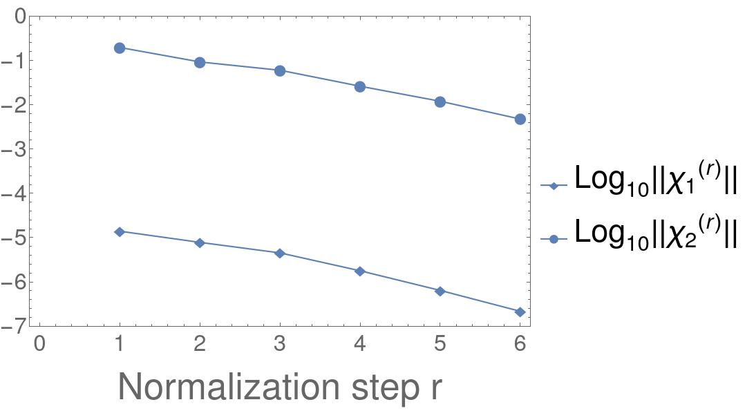
Figure 1: Convergence of the generating functions $\chi_{1}^{(r)}$ and $\chi_{2}^{(r)}$ defined by the normalization algorithm à la Kolmogorov without keeping fixed the angular velocity vector, when it is applied to the 2+2/2 DOF SQPR model without GR corrections in the case corresponding to $(\mathrm{i}_{1}(0),\Omega_{1}(0))=(17^{\circ},5^{\circ})$. The ${\rm Log}_{10}$ of their norms are reported as a function of the normalization step $r\,$.

Moreover, we can express the change of canonical coordinates allowing us to recover the original variables of our problem, i.e., the ones appearing as arguments of the Hamiltonian $\mathcal{H}_{sec,\,2+3/2}\,$, whose expansion is reported in (15). In fact, they can be given as a function of the normalized canonical variables that are listed in the final form of the Hamiltonian (40). Let us recall that this computational procedure “just” requires to compose all the canonical transformations we have previously introduced. Therefore, by using Mathematica as an algebraic manipulator, it has been possible to compute the expansions of such a composition of canonical transformations described in formulæ (21), (22) and (30), in such a way to to construct a semi-analytic (approximate) solution of the equations of motion (12). This corresponds to the invariant KAM torus related to the Kolmogorov normal form (40) which is travelled by quasi-periodic orbits characterized by the angular velocity vector ${\bm{\omega}}^{(*)}\,$, i.e., the motion law can be written as $t\mapsto\big{(}{\bm{p}}(t),{\bm{q}}(t),{\bm{I}}(t),{\bm{\alpha}}(t)\big{)}=\mathscr{C}^{(\mathcal{N}_{s})}\big{(}\mathscr{F}\big{(}\mathcal{T}^{(\tilde{\mathcal{N}}_{s})}({\bm{0}},{\bm{Q}}(0)+{\bm{\omega}}^{(*)}t),P_{5}(0),Q_{5}(0)+\omega_{5}\,t\big{)}\big{)}$. Such a quasi-periodic evolution is plotted (in red) in Figure 2, where one can appreciate the rather good agreement with the numerical integrations of the motion (in black) for what concerns the behavior of both the eccentricity and the inclination of $\upsilon$-And $\mathbf{b}$.

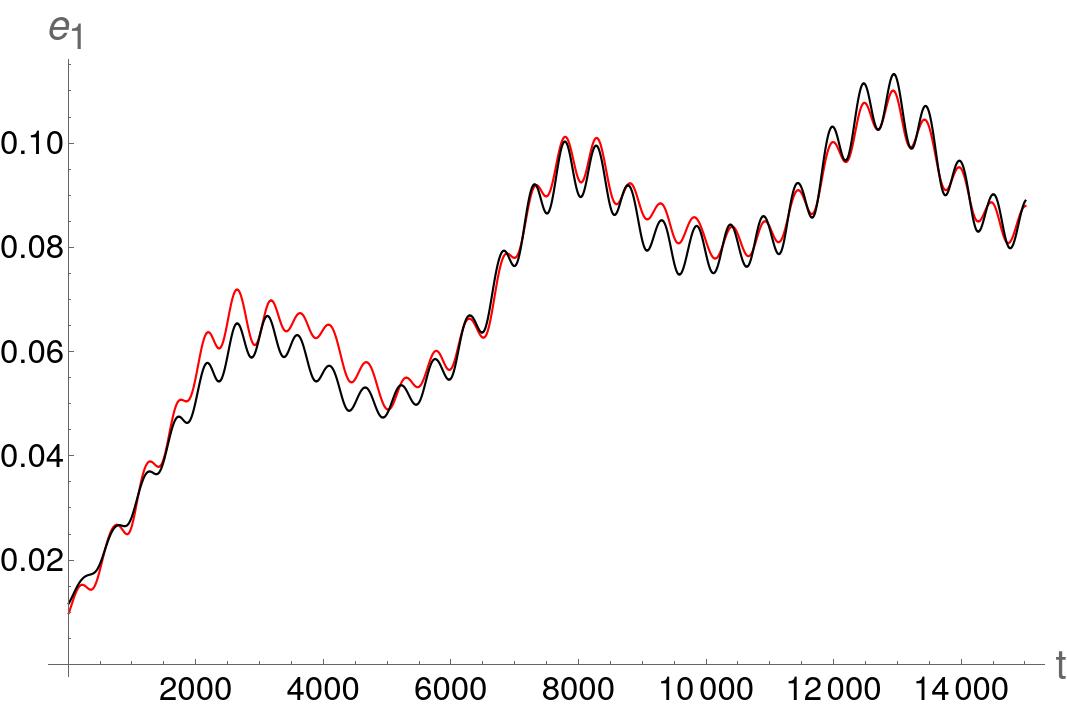
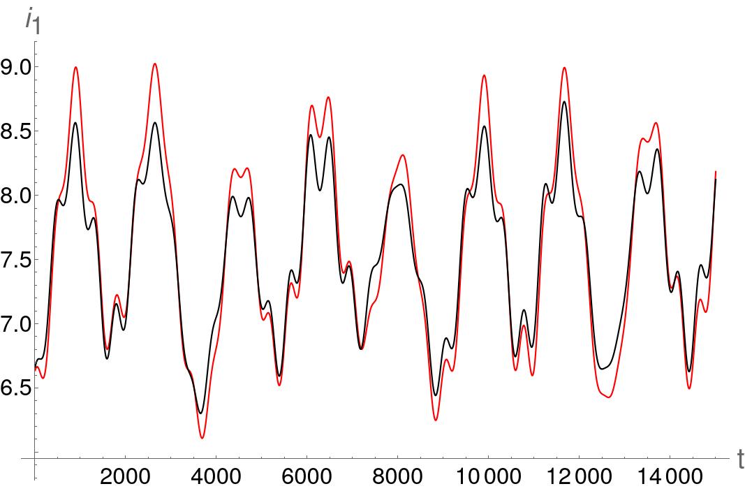
Figure 2: Comparisons between the eccentricity $\mathrm{e}_{1}$ (on the left) and the inclination $\mathrm{i}_{1}$ (on the right) as obtained through the semi-analytical approach (in red) and the numerical one (in black). Both the integration methods consider the case with initial conditions referring to the data reported in Table 2 and they are applied to $2+3/2$ DOF model which does not take into account the effects due to GR. Units of measure for what concerns inclination $\mathrm{i}_{1}$ and time $t$ are degree and year, respectively.

5.2 Computer-Assisted Proofs of existence of KAM tori for the SQPR Hamiltonian models with $2+2/2$ DOF (without GR corrections)

Since we have been able to explicitly perform the normalization procedure à la Kolmogorov just for very few steps of the algorithm by using Mathematica, the expectation of its convergence is not supported in a convincing way by the results discussed in the previous Subsection 5.1. Therefore, we think it is particularly interesting to adopt an approach based on a rigorous Computer-Assisted Proof (hereafter, CAP) for the model introduced above. For such a purpose, it is convenient to run the code CAP4KAM_nDOF which can be downloaded from a publicly available website${{\ref{footnote-CAP4KAM_nDOF}}\atop{\phantom{1}}}$; such a software package is designed to prove the existence of KAM tori for Hamiltonian systems with a number of DOF $n\geq 2$ (while the previous similar version, namely CAP4KAM2D, is limited to the case with 2 DOF). For what concerns the systems described in Subsection 5.1, we apply the CAP to the new initial Hamiltonian

$$H^{(0)}({\bm{P}},{\bm{Q}})=\mathcal{H}^{(\tilde{\mathcal{{N}}}_{S}-1)}({\bm{P}},{\bm{Q}};\,{\bm{I}}_{\ast}^{({3})})$$ (41)

$$=\mathcal{E}^{(\tilde{\mathcal{{N}}}_{S}-1)}({\bm{I}}_{\ast}^{({3})})+\big{(}{\bm{\omega}}^{(\tilde{\mathcal{{N}}}_{S}-1)}({\bm{I}}_{\ast}^{({3})})\big{)}\cdot{\bm{P}}+\sum_{s=0}^{\tilde{\mathcal{N}}_{s}}\sum_{l=2}^{\tilde{\mathcal{N}}_{L}}f_{l}^{(\tilde{\mathcal{{N}}}_{S}-1,\,s)}({\bm{P}},{\bm{Q}};\,{\bm{I}}_{\ast}^{({3})})+\sum_{l=0}^{1}f_{l}^{(\tilde{\mathcal{{N}}}_{S}-1,\,\tilde{\mathcal{N}}_{S})}({\bm{P}},{\bm{Q}};\,{\bm{I}}_{\ast}^{({3})})\,,$$

with $\tilde{N}_{L}=2$, $\tilde{K}=2$ and $\tilde{N}_{S}=7\,$, that corresponds to the Hamiltonian described in formula (36), with $\bar{r}=\tilde{\mathcal{N}}_{S}-1=6$, truncated up to degree $2$ in the actions and to trigonometrical degree $14$ in the angles. This means that we are studying the last Kolmogorov algorithm started at the end of the Newton method, but we consider the Hamiltonian produced at the end of the next to last normalization step. Performing also the last step, of course, would completely remove all the perturbing terms that are represented in our truncated expansions (as already done in Section 5.1, in order to produce Hamiltonian (40)); in such a case an application of a CAP to $\mathcal{H}_{K}^{(\tilde{\mathcal{{N}}}_{S})}$ would be completely pointless. Stopping the preliminary algebraic manipulations that are performed by using Mathematica at the next to last step allows us to consider the main perturbing terms that would make part also of an infinite series expansion of $\mathcal{H}^{(\tilde{\mathcal{{N}}}_{S}-1)}$; therefore, in our opinion this Hamiltonian is a significant starting point and the subsequent normalization procedure is quite challenging.

In the case of the $2+2/2$ DOF Hamiltonian model $\mathcal{H}^{(\tilde{\mathcal{{N}}}_{S}-1)}({\bm{P}},{\bm{Q}};\,{\bm{I}}_{\ast}^{({3})})$ the CAP succeeds in rigorously proving the existence of a set (with positive Lebesgue measure) of KAM tori whose corresponding angular velocity vectors are Diophantine and in an extremely small neighborhood of ${\bm{\omega}}^{(*)}\,$. In the code CAP4KAM_nDOF, that automatically performs the CAP of existence of KAM tori, there are two internal parameters playing a fundamental role, called $R_{\rm{I}}$ and $R_{\rm{II}}$. $R_{\rm{I}}$ refers to the number of normalization steps for which the expansions of the generating functions are explicitly computed; this means that the code explicitly performs $R_{\rm{I}}$ normalization steps of a classical formulation of the Kolmogorov normalization algorithm, computing $H^{(R_{\rm{I}})}$. As a main difference with respect to the computational procedure explained in Subsection 4.2, the classical formulation of the Kolmogorov normalization algorithm takes also into account, at each step $r$, another generating function ${\bm{\xi}}^{(r)}\cdot{\bm{Q}}\,$, in order to keep fixed the wanted angular velocity vector of the quasi-periodic motion on the final torus, namely, ${\bm{\omega}}^{(*)}\,$ (see the original work [22] written by Kolmogorov and [2], [16] for a more modern reformulation that is based on the Lie series method). Instead, $R_{\rm{II}}$ corresponds to the last step for which just the upper bounds of the generating functions are estimated; more precisely, the size of the perturbation is reduced just iterating the estimates of the norms of the terms of order $r$ with $R_{\rm{I}}<r\leq R_{\rm{II}}$. The impact of the choice of the parameters $R_{\rm{I}}$ and $R_{\rm{II}}$ on the performances of this kind of CAPs is widely discussed in [9]. In the former case the values of the parameters that are internal to the CAP and that mostly affect the computational complexity are fixed so that $R_{\rm{I}}=42$ and $R_{\rm{II}}=36000$. The CPU-time needed to complete the CAP is about $74.9$ days on a workstation equipped with processors of type Intel XEON-GOLD 5220 (2.2 GHz).

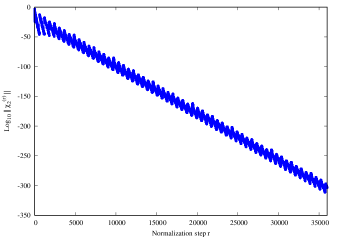
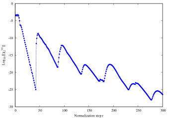
Figure 3: Estimates of the norms (in semi-log scale) of the generating function $\chi_{2}^{(r)}$, as produced during the CAP, using $R_{\rm{I}}=42$ and $R_{\rm{II}}=36000$. On the right, the zoom on the first $300$ normalization steps.

The plot (in semi-log scale) of the estimates of the norm of $\chi_{2}^{(r)}$, reported in the left panel of Fig. 3, shows a regular decreasing behaviour. Moreover, looking at its zoom, i.e., the plot on the right panel, it is evident that such a decrease is steeper up to the step $R_{\rm{I}}$. Then there is a very remarkable leap, due to the transition from the regime of the explicit computation of the generating functions to the one of the pure iteration of the estimates. For increasing values of the normalization step $r$ it is evident the decreasing behaviour of the norm of $\chi_{2}^{(r)}$, with some periodic small jumps. By comparing the plot in the left panel of Fig. 3 with the one on the right, one can easily realize that the behavior of the jumps is similar, but with a different periodicity that is actually induced by another parameter which is internal to the CAP, namely MAXMODKCALC. It has been fixed so as to be equal to $600$; this means that the minimum of the small divisors produced by the solution of the homological equations (see formulæ (31) and (33)) is explicitly computed for Fourier harmonics ${\bm{k}}$ such that $|{\bm{k}}|\leq 600$, while the small divisors are estimated by using the classical Diophantine non-resonance condition for larger values of the trigonometric degree $|{\bm{k}}|$. Due to the extremely small value of the constant $\gamma$ entering in the non-resonance condition (see the following statement 5.1), the corresponding worsening effect is quite evident.

In the case of the model considered in the present section, the computer-assisted proof can be successfully completed by following the approach detailed in [37] so as to apply the KAM theorem in the version described in [36] at the very end of the computational procedure. Our result can be summarized as follows.

Theorem 5.1.

(Computer-assisted) Consider the Hamiltonian $\mathcal{H}^{(6)}\,$, reported in formula (41), or, equivalently, expanded as in (36) with $\bar{r}=6$ and truncated up to degree $2$ in the actions and to trigonometrical degree $14$ in the angles. Let us refer to the ball of radius $\varrho$ centered in ${\bm{\omega}}^{(*)}$, i.e.,

$$\mathcal{S}_{\varrho}({\bm{\omega}}^{(*)})=\{{\bm{\omega}}\in\mathbb{R}^{4}\,:\,\|{\bm{\omega}}-{\bm{\omega}}^{(*)}\|_{\infty}\leq\varrho\}\,,$$

where

$$\omega_{1}^{(*)}=-0.0061397976714045992\,, \omega_{2}^{(*)}=-0.0034842628951575595\,,$$

$$\omega_{3}^{(*)}=-0.0073217663368488322\,, \omega_{4}^{(*)}=-0.0059275598828692194\,.$$

For each ${\bm{\omega}}\in\mathcal{S}_{\varrho}({\bm{\omega}}^{(*)})$ such that it satisfies the Diophantine condition

$$\big{|}{\bm{k}}\cdot{\bm{\omega}}\big{|}\geq\frac{\gamma}{|{\bm{k}}|^{\tau}}\qquad\forall\,{\bm{k}}\in\mathbb{Z}^{4}\setminus\{{\bm{0}}\}\,,$$

with $\varrho=2\times 10^{-15}$, $\gamma=2.9200551117155624\times 10^{-17}$ and $\tau=4\,$, there exists an analytic canonical transformation leading the Hamiltonian $\mathcal{H}^{(6)}$ in the Kolmogorov normal form $\mathcal{H}^{(\infty)}({\bm{P}},{\bm{Q}})=\mathcal{E}^{(\infty)}+{\bm{\omega}}\cdot{\bm{P}}+\mathcal{O}(||{\bm{P}}||^{2})\,$. It is such that, in the new variables, the torus $\{{\bm{P}}={\bm{0}}\,,\,{\bm{Q}}\in\mathbb{T}^{4}\}$ is invariant and travelled by quasi-periodic motions whose corresponding angular velocity vector is equal to ${\bm{\omega}}$.

6 KAM stability of the $2+3/2$ DOF secular model of the innermost exoplanet in the $\upsilon$-Andromedæ system, by including also relativistic effects

Recalling that the innermost planet of the $\upsilon$-Andromedæ system is very close to a star that is about $30\%$ more massive than the Sun, one can easily realize that corrections due to general relativity can play a relevant role. As outlined in Section $6$ of [30], the general relativity induces stabilizing effects on the orbital dynamics of $\upsilon$-And $\mathbf{b}$, producing also a significant modification of the pericenter precession rate. Similarly to what has been done in the previous Section, also for a new model including relativistic corrections, we want to rigorously prove the existence of KAM tori (corresponding to suitably selected orbits) through a computer-assisted proof.

6.1 Secular orbital evolution of $\upsilon$-And $\mathbf{b}$ taking also into account relativistic effects

The secular Hamiltonian, taking into account also general relativistic effects, is defined so that

$$\mathcal{H}^{(GR)}_{sec}=\int_{\mathbb{T}^{3}}\frac{\mathcal{H}_{4BP}}{8\pi^{3}}\,d\lambda_{1}d\lambda_{2}d\lambda_{3}+\int_{\mathbb{T}}\frac{\mathcal{H}_{GR}}{2\pi}\,dM_{1}\,:=\mathcal{H}^{(NG)}_{sec}+\left\langle\mathcal{H}_{{GR}}\right\rangle_{M_{1}}\,,$$ (42)

where $\mathcal{H}_{4BP}$ defines the four body problem (see (6)) and $\mathcal{H}_{GR}$ describes the general (post-Newtonian) relativistic corrections to the Newtonian mechanics. More precisely, $\mathcal{H}^{(NG)}_{sec}$ (recall definition (7)) is explicitely written in equation (8), while the average of the GR contribution with respect to the mean anomaly $M_{1}$ of $\upsilon$-And $\mathbf{b}$ is such that

$$\left\langle\mathcal{H}_{{GR}}\right\rangle_{M_{1}}=-\frac{3\,\mathcal{G}^{2}\,m_{0}^{2}\,m_{1}}{a_{1}^{2}c^{2}\sqrt{1-\mathrm{e}_{1}^{2}}}+\frac{15\,\mathcal{G}^{2}\,m_{0}^{2}\,m_{1}}{8a_{1}^{2}c^{2}}-\frac{\mathcal{G}^{2}\,m_{0}\,m_{1}^{2}}{8a_{1}^{2}c^{2}}\,,$$ (43)

$c$ being the velocity of light in vacuum (see [32] or Appendix E of [29]). Thus, the secular quasi-periodic restricted model of the dynamics of $\upsilon$-And $\mathbf{b}$ which includes corrections due to General Relativity (hereafter, SQPR-GR) can be described by the following $2+3/2$ DOF Hamiltonian:

$$\mathcal{H}^{(GR)}_{sec,\,2+\frac{3}{2}} ({\bm{p}},{\bm{q}},\xi_{1},\eta_{1},P_{1},Q_{1})=\omega_{3}\,p_{3}+\omega_{4}\,p_{4}+\omega_{5}\,p_{5}$$ (44)

$$\qquad\phantom{=}+\mathcal{H}^{(NG)}_{sec}(q_{3},q_{4},q_{5},\xi_{1},\eta_{1},P_{1},Q_{1})+\left\langle\mathcal{H}_{GR}\right\rangle_{M_{1}}(\xi_{1},\eta_{1})\,,$$

where the angular velocity vector ${\bm{\omega}}=(\omega_{3},\omega_{4},\omega_{5}\,)$ is given in (LABEL:freq.fond.CD) and $\mathcal{H}^{(NG)}_{sec}$ can be replaced by $\mathcal{H}^{1-2}_{sec}+\mathcal{H}^{1-3}_{sec}$ appearing in formula (10). Finally, in the framework of this SQPR-GR model, the equations for the orbital motion of the innermost planet can be written as

$$\begin{cases}\dot{q_{3}}=\partial\mathcal{H}^{(GR)}_{sec,2+\frac{3}{2}}/\partial p_{3}=\omega_{3}\\ \dot{q_{4}}=\partial\mathcal{H}^{(GR)}_{sec,2+\frac{3}{2}}/\partial p_{4}=\omega_{4}\\ \dot{q_{5}}=\partial\mathcal{H}^{(GR)}_{sec,2+\frac{3}{2}}/\partial p_{5}=\omega_{5}\\ \dot{\xi}_{1}=-\partial\left(\mathcal{H}_{sec}^{(NG)}(q_{3},q_{4},q_{5},\xi_{1},\eta_{1},P_{1},Q_{1})+\left\langle\mathcal{H}_{GR}\right\rangle_{M_{1}}(\xi_{1},\eta_{1})\right)/\partial\eta_{1}\\ \dot{\eta}_{1}=\partial\left(\mathcal{H}_{sec}^{(NG)}(q_{3},q_{4},q_{5},\xi_{1},\eta_{1},P_{1},Q_{1})+\left\langle\mathcal{H}_{GR}\right\rangle_{M_{1}}(\xi_{1},\eta_{1})\right)/\partial\xi_{1}\\ \dot{P}_{1}=-\partial\mathcal{H}_{sec}^{(NG)}(q_{3},q_{4},q_{5},\xi_{1},\eta_{1},P_{1},Q_{1})/\partial Q_{1}\\ \dot{Q}_{1}=\partial\mathcal{H}_{sec}^{(NG)}(q_{3},q_{4},q_{5},\xi_{1},\eta_{1},P_{1},Q_{1})/\partial P_{1}\end{cases}\,.$$ (45)

Thus, it is possible to numerically integrate the equations of motion (45) of the SQPR-GR model in a similar way to what has been done for the ones already described in Section 2. Finally, let us remark that the invariance law expressed in formula (13) is fulfilled also with $\mathcal{H}^{(GR)}_{sec,\,2+3/2}$, i.e., it holds true also for the Hamiltonian term $\left\langle\mathcal{H}_{{GR}}\right\rangle_{M_{1}}$ which takes into account the relativistic effects on the orbital dynamics of $\upsilon$-And $\mathbf{b}\,$.

6.2 $2+2/2$ DOF Hamiltonian model for the dynamics of $\upsilon$-And $\mathbf{b}$ with relativistic corrections

Proceeding analogously to Sections 3, we start from the SQPR-GR Hamiltonian (44) and we perform the change of variables (14), arriving at the following compact form of the Hamiltonian (similar to formula (16)):

$$\mathcal{H}_{GR}^{(0)}({\bm{p}},{\bm{q}},{\bm{I}},{\bm{\alpha}})=\mathcal{H}^{(GR)}_{sec,\,2+3/2}({\bm{p}},{\bm{q}},{\bm{I}},{\bm{\alpha}}) =\mathcal{E}_{GR}^{(0)}+{\bm{\omega}}^{(0)}\cdot{\bm{p}}+{\bm{\Omega}}_{GR}^{(0)}\cdot{\bm{I}}+\sum_{s=0}^{\mathcal{N}_{S}}\sum_{l=3}^{\mathcal{N}_{L}}h_{l}^{(0,s)}({\bm{q}},{\bm{I}},{\bm{\alpha}})$$ (46)

$$\phantom{=}+\sum_{s=1}^{\mathcal{N}_{S}}\sum_{l=0}^{2}h_{l}^{(0,s)}({\bm{q}},{\bm{I}},{\bm{\alpha}})\,,$$

with $\mathcal{E}_{GR}^{(0)}$ constant, $({\bm{\omega}}^{(0)},{\bm{\Omega}}_{GR}^{(0)})\in\mathbb{R}^{3}\times\mathbb{R}^{2}$ the angular velocity vector and $h_{l}^{(0,s)}\in\mathfrak{P}_{l,sK}$. In agreement with footnote 5, we take $\mathcal{N}_{L}=6$ as maximal power degree in the square root of the actions and we include Fourier terms up to a maximal trigonometric degree of $10$, putting $\mathcal{N}_{S}=5$ and $K=2\,$. Thus, we perform $\mathcal{N}_{S}$ steps of the algorithm constructing the normal form for an elliptic torus (according to Section 3), so as to introduce

$$\mathcal{H}_{GR}^{(\mathcal{N}_{S})}({\bm{p}},{\bm{q}},{\bm{I}},{\bm{\alpha}})=\mathcal{E}_{GR}^{(\mathcal{N}_{S})}+{\bm{\omega}}\cdot{\bm{p}}+{\bm{\Omega}}_{GR}^{(\mathcal{N}_{S})}\cdot{\bm{I}}+\sum_{s=0}^{\mathcal{N}_{S}}\sum_{l=3}^{\mathcal{N}_{L}}h_{l}^{(\mathcal{N}_{S},s)}({\bm{q}},{\bm{I}},{\bm{\alpha}})\,,$$

which is very similar to the Hamiltonian defined in (20). Moreover, proceeding as in Section 4.1, we can perform the change of variables (22), arriving at a Hamiltonian with the same form as that written in formula (23), i.e.,

$$\mathcal{H}_{GR,K}^{(0)}({\bm{P}},{\bm{Q}};\,{\bm{I}}_{\ast})=\mathcal{E}_{GR}^{(0)}({\bm{I}}_{\ast})+\big{(}{\bm{\omega}}_{GR}^{(0)}({\bm{I}}_{\ast})\big{)}\cdot{\bm{P}}+\sum_{s=0}^{\tilde{\mathcal{N}}_{S}}\sum_{l=2}^{\tilde{\mathcal{N}}_{L}}h_{l}^{(0,s)}({\bm{P}},{\bm{Q}};{\bm{I}}_{\ast})+\sum_{s=1}^{\tilde{\mathcal{N}}_{S}}\sum_{l=0}^{1}h_{l}^{(0,s)}({\bm{P}},{\bm{Q}};{\bm{I}}_{\ast})\,,$$ (47)

where $({\bm{P}},{\bm{Q}}):=(P_{1},P_{2},P_{3},P_{4},Q_{1},Q_{2},Q_{3},Q_{4})\,$, and ${\bm{\omega}}_{GR}^{(0)}({\bm{I}}_{\ast})\in\mathbb{R}^{4}$ is defined so that

$$\omega_{GR,\,1}^{(0)}({\bm{I}}_{\ast})=\frac{\partial\left\langle\mathcal{H}_{GR,K}^{(0)}\right\rangle_{{\bm{Q}}}}{\partial P_{1}}\Bigg{|}_{\begin{subarray}{c}P_{1}=0\\ P_{2}=0\end{subarray}}\,, \omega_{GR,\,2}^{(0)}({\bm{I}}_{\ast})=\frac{\partial\left\langle\mathcal{H}_{GR,K}^{(0)}\right\rangle_{{\bm{Q}}}}{\partial P_{2}}\Bigg{|}_{\begin{subarray}{c}P_{1}=0\\ P_{2}=0\end{subarray}}\,,$$ (48)

$$\omega_{GR,3}^{(0)}=\omega_{3}^{(0)}=\omega_{3}-\omega_{5}\,, \omega_{GR,4}^{(0)}=\omega_{4}^{(0)}=\omega_{4}-\omega_{5}\,.$$

Finally, in order to construct the Kolmogorov normal form, we proceed analogously to Section 4.3; thus, we start from $\mathcal{K}^{(0)}({\bm{P}},{\bm{Q}})=\mathcal{H}_{GR,K}^{(0)}({\bm{P}},{\bm{Q}};\,{\bm{I}}_{\ast})$, expressed in formula (47) and we apply the Kolmogorov normalization algorithm (see Section 4.2) in junction with a Newton-like method, performing $\bar{r}=\tilde{\mathcal{N}}_{S}\,$ normalization steps by using Mathematica as an algebraic manipulator. Thus, we arrive at the following Hamiltonian that is truncated and in Kolmogorov normal form:

$$\mathcal{H}_{GR,K}^{(\tilde{\mathcal{{N}}}_{S})}({\bm{P}},{\bm{Q}};\,{\bm{I}}_{\ast}^{({n_{{\cal N}}})})=\mathcal{E}_{GR}^{(\tilde{\mathcal{{N}}}_{S})}({\bm{I}}_{\ast}^{({n_{{\cal N}}})})+\big{(}{\bm{\omega}}_{GR}^{(\tilde{\mathcal{{N}}}_{S})}({\bm{I}}_{\ast}^{({n_{{\cal N}}})})\big{)}\cdot{\bm{P}}+\sum_{s=0}^{\tilde{\mathcal{N}}_{S}}\sum_{l=2}^{\tilde{\mathcal{N}}_{L}}h_{l}^{(\tilde{\mathcal{{N}}}_{S},s)}({\bm{P}},{\bm{Q}};\,{\bm{I}}_{\ast}^{({n_{{\cal N}}})})\,,$$ (49)

which is analogous to the one written in formula (40). In order to find ${\bm{I}}_{\ast}^{({n_{{\cal N}}})}$, we iterate the Newton method until

$$\big{\|}\Delta{\bm{\omega}}^{(GR)}({\bm{I}}_{\ast}^{({n_{{\cal N}}})})\big{\|}_{\infty}=\big{\|}\big{(}\omega_{GR,1}^{(\tilde{\mathcal{N}}_{S})}({{\bm{I}}}_{\ast}^{({n_{{\cal N}}})})-\omega_{GR,1}^{(*)}\,,\,\omega_{GR,2}^{(\tilde{\mathcal{N}}_{S})}({{\bm{I}}}_{\ast}^{({n_{{\cal N}}})})-\omega_{GR,2}^{(*)}\big{)}\big{\|}_{\infty}<10^{-10}\,,$$

where the values of the components of the angular velocity vector ${\bm{\omega}}_{GR}^{(*)}\,$ are such that

$$\omega_{GR,1}^{(*)}=\omega_{GR,1}-\omega_{5}\,,\quad\omega_{GR,2}^{(*)}=\omega_{GR,2}-\omega_{5}\,,\quad\omega_{GR,3}^{(*)}=\omega_{3}-\omega_{5}\,,\quad\omega_{GR,4}^{(*)}=\omega_{4}-\omega_{5}\,.$$ (50)

In the previous formula, the values of $(\omega_{3},\omega_{4},\omega_{5})\in\mathbb{R}^{3}$, are related to the fundamental periods of the two outer exoplanets and are given in equation (LABEL:freq.fond.CD), while $\omega_{GR,1}$ and $\omega_{GR,2}$ are the values of the fundamental angular velocities as obtained by the frequency analysis method when it is applied to the discretized signals $t\mapsto\sqrt{2\Lambda_{1}}\,\sqrt{1-\sqrt{1-\big{(}\mathrm{e}_{1}(t)\big{)}^{2}}}\,e^{-i\varpi_{1}(t)}\,$, $t\mapsto 2\sqrt{\Lambda_{1}}\,\sqrt[4]{1-\big{(}\mathrm{e}_{1}(t)\big{)}^{2}}\,\sin\big{(}\frac{\mathrm{i}_{1}(t)}{2}\big{)}\,e^{-i\Omega_{1}(t)}$, respectively, which are produced by the numerical integration of the original $2+3/2$ DOF Hamiltonian model with GR corrections, defined in formula (44).

6.3 Results produced by the semi-analytic integration of the SQPR Hamiltonian model with $2+2/2$ DOF and GR corrections

We now start considering the numerical integration of secular quasi-periodic restricted Hamiltonian which has $2+3/2$ DOF and takes into account the relativistic effects, namely $\mathcal{H}^{(GR)}_{sec,\,2+\frac{3}{2}}$ written in (44), whose corresponding equations of motion are reported in formula (45). We consider the initial conditions which are reported in Table 3 and approximately correspond to the center of the stability region according to the numerical study described in Section 6 of [30].

	$\upsilon$-And $\bf{b}$
$m\,[M_{J}]$	$0.674$
$a(0)\,[{\rm AU}]$	$0.0594$
$\mathrm{e}(0)$	$0.011769$
$\mathrm{i}(0)\,[^{\circ}]$	$20.$
$M(0)\,[^{\circ}]$	$103.53$
$\omega(0)\,[^{\circ}]$	$51.14$
$\Omega(0)\,[^{\circ}]$	$0.$

Table 3: Values of the initial orbital parameters for $\upsilon$-And $\mathbf{b}$. The chosen value of the mass is the minimal one according to [31]. The values $a_{1}(0)\,$, $\mathrm{e}_{1}(0)\,$, $M_{1}(0)$ and $\omega_{1}(0)$ are reported from the stable prograde trial PRO2 of [12] (Table $3\,$). The values of initial inclination and longitude of the node (denoted with $\mathrm{i}_{1}(0)$ and $\Omega_{1}(0)$, respectively) are taken from [30]; see the text for more details. The corresponding initial orbital parameters in the Laplace reference frame can be easily determined (see, e.g., [29]).

For what concerns the semi-analytical approach, we start from the $2+2/2$DOF Hamiltonian, written in formula (49). For the construction of the Kolmogorov normal form (without fixing the angular velocity vector, as explained in Section 4.2 and applied in the previous Section), we adopt $\tilde{\mathcal{N}}_{L}=2\,$, $\tilde{K}=2\,$, $\tilde{\mathcal{N}}_{S}=6\,$ as parameters ruling the truncations of the expansions. In particular, ${n_{{\cal N}}}=2$ iterations of the Newton method are enough to reach the condition $\|{\bm{\omega}}_{GR}^{(\tilde{\mathcal{{N}}}_{S})}({{\bm{I}}}_{\ast}^{(2)})-{\bm{\omega}}_{GR}^{(*)}\|_{\infty}<10^{-10}$, which allows us to successfully conclude the search for the initial translation vector that approximates well enough the one we are looking for, namely the unknown ${{\bm{I}}}_{\ast}\,$. We focus again on the last Kolmogorov normalization that is performed at the end of the Newton method, i.e., the one corresponding to the initial translation vector ${{\bm{I}}}_{\ast}^{(2)}$. Looking at Figure 4, once again we can appreciate a rather regular and sharp decay of the norms of the generating functions $\chi_{1}^{(r)}$ and $\chi_{2}^{(r)}$ .

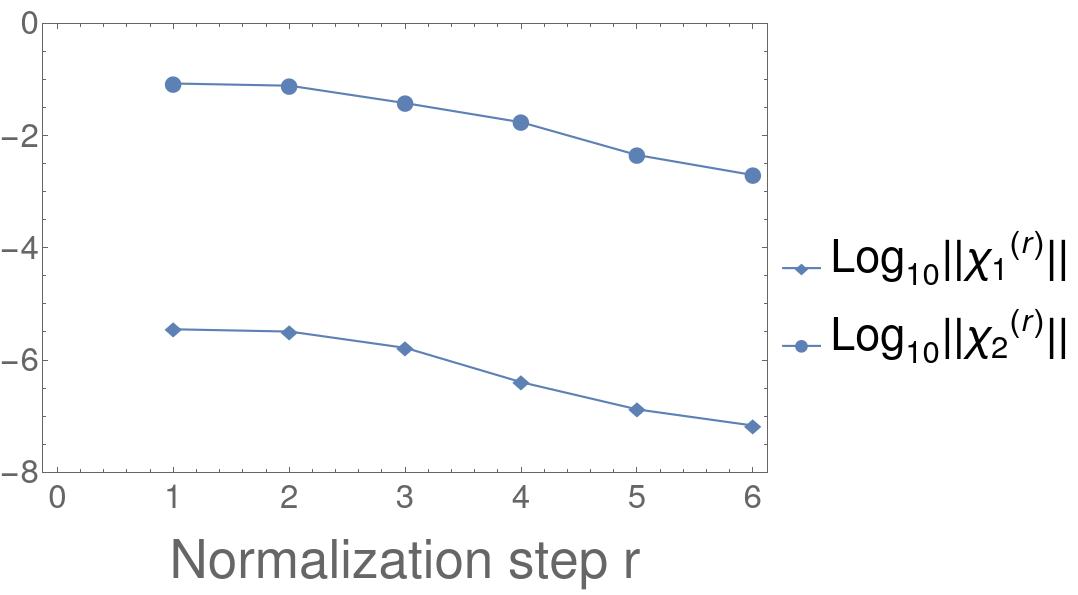
Figure 4: Convergence of the generating functions $\chi_{1}^{(r)}$ and $\chi_{2}^{(r)}$ defined by the normalization algorithm à la Kolmogorov without keeping fixed the angular velocity vector, when it is applied to the 2+2/2 DOF SQPR model with GR corrections and is performed in the case corresponding to $(\mathrm{i}_{1}(0),\Omega_{1}(0))=(20^{\circ},0^{\circ})$. The ${\rm Log}_{10}$ of their norms are reported as a function of the normalization step $r\,$.

Following again the approach described in the previous Subsection 5.1, we can construct a semi-analytic (approximate) solution of the equations of motion (45) which here corresponds to a quasi-periodic orbit whose angular velocity vector is now denoted with ${\bm{\omega}}_{GR}^{(*)}\,$. Such a quasi-periodic evolution is plotted (in red) in Figure 5, where one can appreciate that there is rather good agreement with the numerical integrations of the motion (in black) for what concerns the behavior of both the eccentricity and the inclination of $\upsilon$-And $\mathbf{b}$ (apart a small shift of the two plots reported in the left panel).

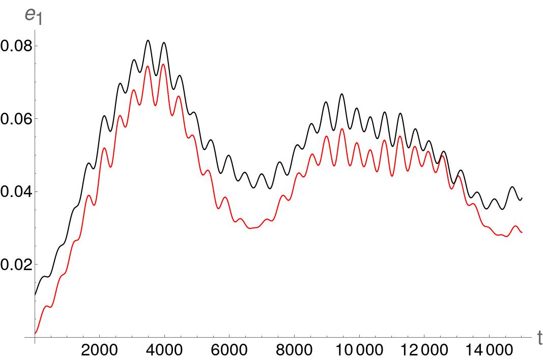
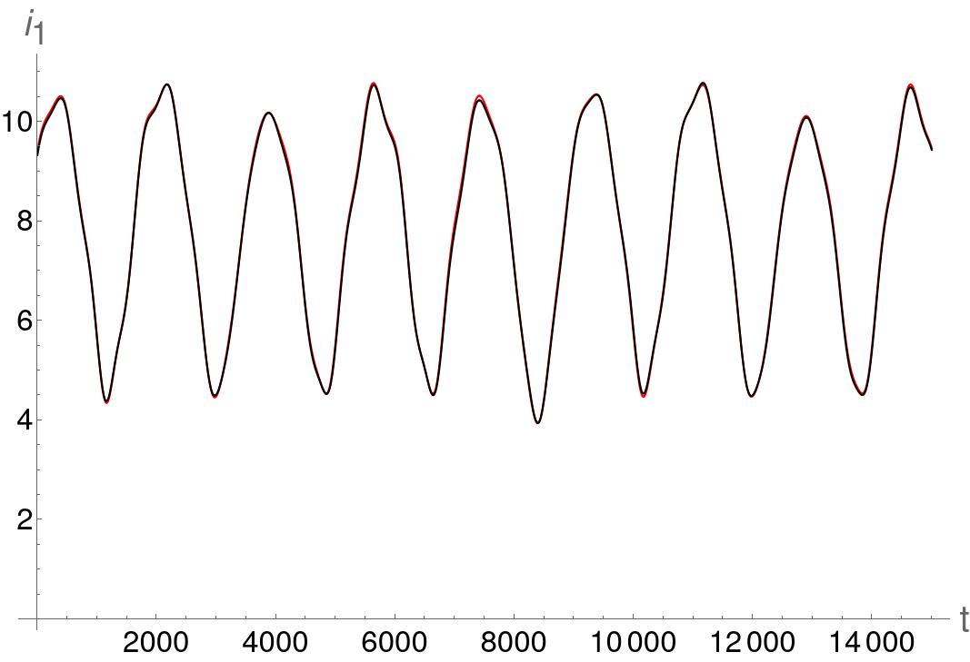
Figure 5: Comparisons between the eccentricity $\mathrm{e}_{1}$ (on the left) and the inclination $\mathrm{i}_{1}$ (on the right) as obtained through the semi-analytical approach (in red) and the numerical one (in black). Both the integration methods consider the case with initial conditions referring to the data reported in Table 3 and they are applied to $2+3/2$ DOF model which does take into account the effects due to GR. Units of measure for what concerns inclination $\mathrm{i}_{1}$ and time $t$ are degree and year, respectively.

6.4 Computer-Assisted Proofs of existence of KAM tori for the SQPR Hamiltonian models with $2+2/2$ DOF and GR corrections

In a similar way to what has been done in Section 5.2, we want to adopt an approach based on rigorous CAPs also to the case described above, i.e., adding also the relativistic effects on the dynamics of $\upsilon$-And $\mathbf{b}$.

Thus, we use the publicly available software package${{\ref{footnote-CAP4KAM_nDOF}}\atop{\phantom{1}}}$ that is designed for performing CAPs, in order to apply it to the new initial Hamiltonian

$$H_{GR}^{(0)}({\bm{P}},{\bm{Q}})=\mathcal{H}_{GR}^{(\tilde{\mathcal{{N}}}_{S}-1)}({\bm{P}},{\bm{Q}};\,{\bm{I}}_{\ast}^{({2})})$$ (51)

$$=\mathcal{E}_{GR}^{(\tilde{\mathcal{{N}}}_{S}-1)}({\bm{I}}_{\ast}^{({2})})+\big{(}{\bm{\omega}}_{GR}^{(\tilde{\mathcal{{N}}}_{S}-1)}({\bm{I}}_{\ast}^{({2})})\big{)}\cdot{\bm{P}}+\sum_{s=0}^{\tilde{\mathcal{N}}_{s}}\sum_{l=2}^{\tilde{\mathcal{N}}_{L}}h_{l}^{(\tilde{\mathcal{{N}}}_{S}-1,\,s)}({\bm{P}},{\bm{Q}};\,{\bm{I}}_{\ast}^{({2})})+\sum_{l=0}^{1}h_{l}^{(\tilde{\mathcal{{N}}}_{S}-1,\,\tilde{\mathcal{N}}_{S})}({\bm{P}},{\bm{Q}};\,{\bm{I}}_{\ast}^{({2})})\,,$$

with $\tilde{N}_{L}=2$, $\tilde{K}=2$ and $\tilde{N}_{S}=7\,$. As remarked in Section 5.2, performing also the last step would completely remove all the perturbing terms that are represented in our truncated expansions, making the application of a CAP to $\mathcal{H}_{GR}^{(\tilde{\mathcal{{N}}}_{S})}$ meaningless.

In the case of the $2+2/2$ DOF Hamiltonian model $\mathcal{H}^{(\tilde{\mathcal{{N}}}_{S}-1)}({\bm{P}},{\bm{Q}};\,{\bm{I}}_{\ast}^{({2})})$ (which consider also relativistic effects, described in formula (51)) the CAP succeeds in rigorously proving the existence of a set (with positive Lebesgue measure) of KAM tori whose corresponding angular velocity vectors are Diophantine and in an extremely small neighborhood of ${\bm{\omega}}_{GR}^{(*)}\,$. In the present case the values of the parameters that are internal to the CAP and that mostly affect the computational complexity are fixed so that $R_{\rm{I}}=38$ and $R_{\rm{II}}=54000$. The CPU-time needed to complete the CAP is about $32.2$ days on a workstation equipped with processors of type Intel XEON-GOLD 5220 (2.2 GHz). It is amazing that our CAP in the present case needs just $\simeq 43\%$ of CPU-time with respect to the application described in Section 5.2. This is mainly due to the fact that the generating functions $\chi_{1}^{(r)}$ and $\chi_{2}^{(r)}$ (when they are explicitly computed for $1\leq r\leq R_{\rm{I}}$) contain less terms in their Fourier expansions and their norms decrease more sharply. Also this phenomenon can be seen as a byproduct of the stabilizing effect due to the relativistic corrections.

The plot (in semi-log scale) of the estimates of the norm of $\chi_{2}^{(r)}$, reported in Fig. 6, shows a regular decreasing behaviour. Moreover, looking at the plot on the right, it is evident that such a decrease is steeper up to the step $R_{\rm{I}}$. As in Fig. 3, both in the left panel of Fig. 6 and in the one on the right, we can appreciate the periodicity of small jumps, that depend on the parameters MAXMODKCALC (here fixed so as to be equal to $550$) and $R_{\rm{I}}\,$, respectively; both of these parameters are internal to the CAP.

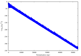
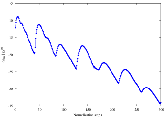
Figure 6: Estimates of the norms (in semi-log scale) of the generating function $\chi_{2}^{(r)}$, as produced during the CAP, using $R_{\rm{I}}=38$ and $R_{\rm{II}}=54000$. On the right, the zoom on the first $300$ normalization steps.

Also in this case case, the computer-assisted proof can be successfully completed by applying the KAM theorem in the version described in [36]. Our final result is summarized by the following statement.

Theorem 6.1.

(Computer-assisted) Consider the Hamiltonian $\mathcal{H}_{GR}^{(6)}\,$, reported in formula (51). Let us introduce the ball of radius $\varrho$ centered in ${\bm{\omega}}_{GR}^{(*)}$, i.e.,

$$\mathcal{S}_{\varrho}({\bm{\omega}}_{GR}^{(*)})=\{{\bm{\omega}}\in\mathbb{R}^{4}\,:\,\|{\bm{\omega}}-{\bm{\omega}}_{GR}^{(*)}\|_{\infty}\leq\varrho\}\,,$$

where

$$\omega_{GR,1}^{(*)}=-0.0064644895081070399\,, \omega_{GR,2}^{(*)}=-0.0034914960690528801\,,$$

$$\omega_{GR,3}^{(*)}=-0.0073217663368488322\,, \omega_{GR,4}^{(*)}=-0.0059275598828692194\,.$$

For each ${\bm{\omega}}\in\mathcal{S}_{\varrho}({\bm{\omega}}_{GR}^{(*)})$ such that it satisfies the Diophantine condition

$$\big{|}{\bm{k}}\cdot{\bm{\omega}}\big{|}\geq\frac{\gamma}{|{\bm{k}}|^{\tau}}\qquad\forall\,{\bm{k}}\in\mathbb{Z}^{4}\setminus\{{\bm{0}}\}\,,$$

with $\varrho=2\times 10^{-15}$, $\gamma=2.6761115506846878\times 10^{-17}$ and $\tau=4\,$, there exists an analytic canonical transformation leading $\mathcal{H}_{GR}^{(6)}$ in a Kolmogorov normal form for which there is a torus which is invariant with respect to the corresponding Hamiltonian flow and is travelled by quasi-periodic motions whose corresponding angular velocity vector is equal to ${\bm{\omega}}$.

References

- [1] K. Batygin, A. Morbidelli, and M. J. Holman. Chaotic disintegration of the inner Solar System. Astrophysical Journal, 799(2):120, 2015.
- [2] G. Benettin, L. Galgani, A. Giorgilli, and J.-M. Strelcyn. A proof of Kolmogorov’s theorem on invariant tori using canonical transformations defined by the Lie method. Nuovo Cimento, 79:201–223, 1984.
- [3] R. P. Butler, G. W. Marcy, D. A. Fischer, T. M. Brown, A. R. Contos, S. G. Korzennik, P. Nisenson, and R. W. Noyes. Evidence for multiple companions to Andromedae. The Astrophysical Journal, 526(2):916, dec 1999.
- [4] R. Calleja, A. Celletti, and R. de la Llave. KAM quasi-periodic solutions for the dissipative standard map. Communications in Nonlinear Science and Numerical Simulation, 106:106111, 2022.
- [5] R. Calleja, A. Celletti, J. Gimeno, and R. de la Llave. KAM quasi-periodic tori for the dissipative spin–orbit problem. Communications in Nonlinear Science and Numerical Simulation, 106:106099, 2022.
- [6] C. Caracciolo and U. Locatelli. Elliptic tori in FPU non-linear chains with a small number of nodes. Communications in Nonlinear Science and Numerical Simulation, 97:105759, 2021.
- [7] C. Caracciolo, U. Locatelli, M. Sansottera, and M. Volpi. Librational KAM tori in the secular dynamics of the Andromedæ planetary system. Monthly Notices of the Royal Astronomical Society, 510(2):2147–2166, 2022.
- [8] A. Celletti and L. Chierchia. KAM stability and celestial mechanics. Memoirs of the American Mathematical Society, 187(878), 2007.
- [9] A. Celletti, A. Giorgilli, and U. Locatelli. Improved estimates on the existence of invariant tori for Hamiltonian systems. Nonlinearity, 13(2):397, 2000.
- [10] S. Curiel, J. Cantó, L. Georgiev, C. Chávez, and A. Poveda. A fourth planet orbiting Andromedae. Astronomy & Astrophysics, 525:A78, 2011.
- [11] V. Danesi, U. Locatelli, and M. Sansottera. Existence proof of librational invariant tori in an averaged model of HD60532 planetary system. Celestial Mechanics and Dynamical Astronomy, 135(3):24, 2023.
- [12] R. Deitrick, R. Barnes, B. McArthur, T. R. Quinn, R. Luger, A. Antonsen, and G. F. Benedict. The three-dimensional architecture of the Andromedae planetary system. The Astrophysical Journal, 798(1):46, 2015.
- [13] J.-L. Figueras, A. Haro, and A. Luque. Rigorous computer-assisted application of KAM theory: a modern approach. Foundations of Computational Mathematics, 17(5):1123–1193, 2017.
- [14] A. Giorgilli. Notes on exponential stability of Hamiltonian systems. Pubblicazioni della Classe di Scienze, Scuola Normale Superiore, Pisa. Centro di Ricerca Matematica ”Ennio De Giorgi”, 2003.
- [15] A. Giorgilli. Notes on Hamiltonian Dynamical Systems, volume 102. Cambridge University Press, 2022.
- [16] A. Giorgilli and U. Locatelli. Kolmogorov theorem and classical perturbation theory. J. of App. Math. and Phys. (ZAMP), 48:220–261, 1997.
- [17] A. Giorgilli, U. Locatelli, and M. Sansottera. Secular dynamics of a planar model of the Sun-Jupiter-Saturn-Uranus system; effective stability in the light of Kolmogorov and Nekhoroshev theories. Regular and Chaotic Dynamics, 22:54–77, 2017.
- [18] W. Gröbner. Die Lie-reihen und ihre Anwendungen, volume 3. Deutscher Verlag der Wissenschaften, 1967.
- [19] N. H. Hoang, F. Mogavero, and J. Laskar. Long-term instability of the inner Solar System: numerical experiments. Monthly Notices of the Royal Astronomical Society, 514(1):1342–1350, 2022.
- [20] T. Kapela, M. Mrozek, D. Wilczak, and P. Zgliczynski. CAPD::DynSys: A flexible C++ toolbox for rigorous numerical analysis of dynamical systems. Communications in Nonlinear Science and Numerical Simulation, 101:105578, 2021.
- [21] T. Kapela, D. Wilczak, and P. Zgliczynski. Recent advances in a rigorous computation of Poincaré maps. Communications in Nonlinear Science and Numerical Simulation, 110:106366, 2022.
- [22] A. Kolmogorov. Preservation of conditionally periodic movements with small change in the Hamilton function. Dokl. Akad. Nauk SSSR, 98:527–530, 1954; English translation in Casati, G. and Ford, J. (eds.): Lecture Notes in Physics, 93:51–56, 1979.
- [23] J. Laskar. Large scale chaos and marginal stability in the solar system. Celestial Mechanics and Dynamical Astronomy, 64:115–162, 1996.
- [24] J. Laskar. Frequency map analysis and quasiperiodic decompositions. In E. Lega, D. Benest, and C. Froeschlé, editors, Hamiltonian systems and Fourier analysis: new prospects for gravitational dynamics. Cambridge Scientific Pub Ltd, 2005.
- [25] J. Laskar and P. Robutel. High order symplectic integrators for perturbed Hamiltonian systems. Celestial Mechanics and Dynamical Astronomy, 80(1):39–62, 2001.
- [26] U. Locatelli, C. Caracciolo, M. Sansottera, and M. Volpi. A numerical criterion evaluating the robustness of planetary architectures; applications to the andromedæ system. Proceedings of the International Astronomical Union, 15(S364):65–84, 2021.
- [27] U. Locatelli, C. Caracciolo, M. Sansottera, and M. Volpi. Invariant KAM tori: from theory to applications to exoplanetary systems. Springer Proceedings in Mathematics and Statistics, 399:1–45, 2022.
- [28] U. Locatelli and A. Giorgilli. Invariant tori in the secular motions of the three-body planetary systems. Celestial Mechanics and Dynamical Astronomy, 78(1):47–74, 2000.
- [29] R. Mastroianni. Hamiltonian secular theory and KAM stability in exoplanetary systems with 3D orbital architecture. PhD Thesis, Dep. of Mathematics “Tullio-Levi Civita”, Univ. of Padua, 2023.
- [30] R. Mastroianni and U. Locatelli. Secular orbital dynamics of the innermost exoplanet of the -Andromedæ system. Celestial Mechanics and Dynamical Astronomy, 135(3):28, 2023.
- [31] B. E. McArthur, G. F. Benedict, R. Barnes, E. Martioli, S. Korzennik, E. Nelan, and R. P. Butler. New observational constraints on the Andromedae system with data from the Hubble Space Telescope and Hobby-Eberly Telescope. The Astrophysical Journal, 715(2):1203–1220, 2010.
- [32] C. Migaszewski and K. Goździewski. Secular dynamics of a coplanar, non-resonant planetary system under the general relativity and quadrupole moment perturbations. Monthly Notices of the Royal Astronomical Society, 392(1):2–18, 2009.
- [33] A. Morbidelli. Modern celestial mechanics: aspects of solar system dynamics. 2002.
- [34] A. Morbidelli and A. Giorgilli. Superexponential stability of KAM tori. Journal of Statistical Physics, 78:1607–1617, 1995.
- [35] C. D. Murray and S. F. Dermott. Solar system dynamics. Cambridge university press, 1999.
- [36] L. Stefanelli and U. Locatelli. Kolmogorov’s normal form for equations of motion with dissipative effects. Discrete Contin. Dynam. Systems, 17(7):2561–2593, 2012.
- [37] L. Valvo and U. Locatelli. Hamiltonian control of magnetic field lines: Computer assisted results proving the existence of KAM barriers. Journal of Computational Dynamics, 9:505–527, 2022.