Astrophysical black holes: theory and observations

Abstract

These notes cover part of the lectures presented by Andrea Maselli for the 59th Winter School of Theoretical Physics and third COST Action CA18108 Training School ‘Gravity – Classical, Quantum and Phenomenology’. The school took place at Pałac Wojanów, Poland, from February 12th to 21st, 2023. The lectures focused on some key aspects of black hole physics, and in particular on the dynamics of particles and on the scattering of waves in the Schwarzschild spacetime. The goal of the course was to introduce the students to the concept of black hole quasi normal modes, to discuss their properties, their connection with the geodesic motion of massless particles, and to provide numerical approaches to compute their actual values.

1 Introduction

With nearly one hundred events from coalescing binaries detected by LIGO-Virgo-KAGRA [1], gravitational-wave (GW) observations have shaped a novel path for studying high-energy phenomena in our Universe. The number of observations is expected to rise with current interferometers at their design sensitivity, growing by orders of magnitude with the next generations of ground and space facilities, such as the Einstein Telescope [2], Cosmic Explorer [3], and the LISA satellite [4]. The loudness of the signals detected by such network of GW observatories will turn GW into a new tool for precision (astro)physics, enabling the exploration of various scientific phenomena. Primary objectives of this quest include testing the foundations of General Relativity (GR) and understanding the nature of gravity in strong field and highly dynamic scenarios [5, 6, 7, 8].

One of the most promising approaches for testing gravity, particularly a key prediction of GR, namely, the uniqueness of Kerr black holes (BHs), revolves around the so-called black hole spectroscopy. This approach exploits the signal following a binary merger, known as the ringdown, which can be described in terms of series of damped oscillations with characteristic frequencies called quasi-normal modes (QNMs). In General Relativity, QNMs are uniquely determined by the mass and angular momentum of the BH [9, 10, 11]. Measuring the frequency and damping time of a single QNM allows for the determination of the BH mass and spin, while multiple modes could provide null-hypothesis tests of GR [12, 13, 14]. This correspondence also makes QNMs a versatile diagnostic tool, leading, for example, to consistency checks between inspiral and post-merger parameters inferred from binary events, searches for exotic states of matter at the horizon scale, and detection of signatures of modified theories of gravity [7, 15, 16]. This plethora of opportunities sets the foundations of QNMs spectroscopy, in complete analogy with the longstanding efforts devoted to atomic and condensed matter physics.

In these notes, we outline the essential components necessary for calculating the BH response to an external perturbation, including its QNMs spectrum. We begin by examining the fundamental properties of stationary BH solutions in GR (Section 2) and their geodesic structure (Section 3). Subsequently, our focus shifts to Section 4, where we delve into the formalism required to compute relativistic perturbations of Schwarzschild BHs, further explored in Section 5. Throughout, we adopt geometric units, $c=G=1$.

2 The Schwarzschild solution

Historically, the Schwarzschild metric represents the first exact solution of the Einstein equations, alongside Minkowski flat spacetime, discovered by Karl Schwarzschild in 1916, just one year after the publication of GR. The Schwarzschild metric is a non-trivial solution of the Einstein vacuum field equations

$$R_{\mu\nu}=0\ ,$$ (1)

describing a Ricci-flat manifold (hereafter, lowercase Greek letters represent spacetime indices $\mu,\nu,\dotsc=0,1,2,3$). This metric determines the gravitational field generated by a static, spherically symmetric, electrically uncharged, and non-rotating mass, assuming a vanishing cosmological constant. From a physical perspective, the Schwarzschild metric finds various applications, particularly in describing the vacuum outer region of non-spinning stars and planets.

2.1 The Birkhoff theorem

The Schwarzschild spacetime comes with a remarkable feature dictated by the Birkhoff theorem. This theorem asserts that the Schwarzschild metric is the unique vacuum solution with spherical symmetry, which is also static. In the following we shall provide the proof of the theorem.

Consider a $(3+1)$-dimensional spacetime exhibiting spatial spherical symmetry, namely, a manifold with the three-dimensional special orthogonal group $SO(3)$ (representing rotations in three-dimensional Euclidean space) as its group of symmetries. The three generators of the action of $SO(3)$ on the spacetime are the following [17]:

$$J_{1} =x^{2}\,\partial_{3}-x^{3}\,\partial_{2}=-\sin\varphi\,\partial_{\theta}-\cot\theta\cos\varphi\,\partial_{\varphi}\ ,$$ (2)

$$J_{2} =x^{3}\,\partial_{1}-x^{1}\,\partial_{3}=\cos\varphi\,\partial_{\theta}-\cot\theta\sin\varphi\,\partial_{\varphi}\ ,$$

$$J_{3} =x^{1}\,\partial_{2}-x^{2}\,\partial_{1}=\partial_{\varphi}\ ,$$

where $x^{i}$ are Cartesian coordinates (with spatial indices $i,j,\dotsc=1,2,3$), and $r\in[0,+\infty)$, $\theta\in[0,\pi]$, $\varphi\in[0,2\pi)$ are spherical coordinates. The transformation between Cartesian and spherical coordinates is given by the usual expressions

$$x^{1}=r\sin\theta\cos\varphi\ ,\qquad x^{2}=r\sin\theta\sin\varphi\ ,\qquad x^{3}=r\cos\theta\ .$$ (3)

The generators $J_{i}$ satisfy the commutation relations

$$[J_{i},J_{j}]=\varepsilon_{ijk}J_{k}\ ,$$ (4)

where $\varepsilon_{ijk}$ is the Levi-Civita symbol. The generators of symmetries are also known as Killing vectors since they satisfy the Killing equation:

$$\mathcal{L}_{J}g_{\mu\nu}=\nabla_{\mu}J_{\nu}+\nabla_{\nu}J_{\mu}=0\ ,$$ (5)

where $\mathcal{L}_{J}$ is the Lie derivative along the Killing vector $J$ (in this case, a generator of $SO(3)$), and $\nabla_{\mu}$ represents the covariant derivative associated with the spacetime metric $g_{\mu\nu}$. In other words, Killing vectors generate transformations that preserve the metric, defining isometries.

A three-dimensional space with $SO(3)$ as it isometry group can be foliated into two-spheres centered at the same origin but with varying radii. These two-spheres represent the homogeneous spaces of the $SO(3)$ group, meaning that any point on the sphere can be reached through a rotation starting from an arbitrarily chosen origin. This procedure, which cannot be applied to the center of the spheres, where the homogeneous space becomes zero-dimensional, is graphically depicted in Fig. 1. Each of these two-dimensional homogeneous spaces corresponds to a standard two-sphere with a metric, in spherical coordinates, given by:

$$ds^{2}=r^{2}d\Omega^{2}=r^{2}d\theta^{2}+r^{2}\sin^{2}\theta\,d\varphi^{2}\ ,$$ (6)

where $r$ represents the radius of the sphere (constant within each sphere).

Figure 1: Foliation of $\mathbb{R}^{3}$ (minus the origin) by two-spheres.

The process of spacetime foliation into maximally symmetric submanifolds, such as the two-spheres in our scenario, allows us to choose coordinates adapted to this foliation. For instance, consider a generic $n$-dimensional manifold foliated by $m$-dimensional submanifolds. We can use a set of $m$ coordinates ${u^{i}}$, where $i=1,\dotsc,m$, to represent the submanifold, and another set of $m-n$ coordinates ${v^{a}}$, where $a=1,\dotsc,m-n$, to specify the particular submanifold we are on. By combining these two sets of coordinates, we can coordinatize the entire manifold as ${u^{i},v^{a}}$. Remarkably, when these submanifolds are maximally symmetric, a theorem (for the proof, see Ref. [18]) guarantees that the metric can be expressed in the following form:

$$ds^{2}=g_{\mu\nu}dx^{\mu}dx^{\nu}=g_{ab}(v)dv^{a}dv^{b}+f(v)h_{ij}(u)du^{i}du^{j}\ ,$$ (7)

where $h_{ij}$ represents the metric of the maximally symmetric submanifold. We can make two important observations based on the form of Eq. (7): (i) there are no mixed terms $dv^{i}du^{a}$, namely the metric $g_{\mu\nu}$ is a block-diagonal matrix, and (ii) both $g_{ab}$ and $f$ depends uniquely on the variables $v^{a}$. The absence of mixed terms indicates that the submanifolds are consistently aligned throughout the entire space, which allows us to move across them while crossing points with the same $u^{i}$ coordinates but on different submanifolds. Additionally, the fact that $g_{ab}$ and $f$ do not depend on $u^{i}$ implies that the metric of different submanifolds remains the same (up to a numerical factor), as the coordinates $v^{a}$ remain constant on a given submanifold.

In our case, the submanifold coordinates are given by the spherical coordinates $\theta$ and $\varphi$, and the corresponding metric is $h_{ij}(u)du^{i}du^{j}=d\Omega^{2}$. Consequently, we can express the metric of the entire spacetime as follows:

$$ds^{2}=g_{11}(v)dv^{1}dv^{1}+2g_{12}(v)dv^{1}dv^{2}+g_{22}(v)dv^{2}dv^{2}+r^{2}(v)d\Omega^{2}\ ,$$ (8)

where we have redefined the yet-to-be-determined function as $f(v)=r^{2}(v)$. To simplify the calculations, we can invert the function $r(v^{1},v^{2})$ with respect to one of the two variables on which it depends, for instance, with respect to $v^{1}$. Moreover, we shall find another function $t(v^{2},r)$ such that, when expressed in terms of $t$ and $r$, the metric does not exhibit cross terms like $dtdr$. It can be shown (see Ref. [19]) that this is always possible, which allows us to recast the metric in the following form:

$$ds^{2}=a_{1}(t,r)dt^{2}+a_{2}(t,r)dr^{2}+r^{2}d\Omega^{2}\ ,$$ (9)

The variable $r$ works as a scale factor in front of the metric of the two-sphere. This is also the case in the Minkowski spacetime in spherical coordinates, where $ds=-dt^{2}+dr^{2}+r^{2}d\Omega^{2}$. The latter can indeed be obtained by setting $a_{1}=-1$ and $a_{2}=1$ in Eq. (9), with the minus sign arising from the fact that the Minkowski spacetime is a Lorentzian manifold with signature $(-,+,+,+)$. Following the same procedure for our case, we can fix $a_{1}$ and $a_{2}$ such that

$$ds^{2}=-e^{2\alpha(t,r)}dt^{2}+e^{2\beta(t,r)}dr^{2}+r^{2}d\Omega^{2}\ .$$ (10)

We remark that the form of Eq. (10) is only dictated by the assumption of spherical symmetry, and depends on the two functions $\alpha$ and $\beta$, that can be determined by solving the Einstein vacuum field equations (1).

To solve the Einstein equations, we need to explicitly calculate the components of the Ricci tensor $R_{\mu\nu}$, derived from the Riemann curvature tensor $\tensor{R}{{}^{\mu}_{\nu}{}_{\sigma}{}_{\rho}}$:

$$R_{\mu\nu}=\tensor{R}{{}^{\sigma}_{\mu}{}_{\sigma}{}_{\nu}}\ ,\qquad\tensor{R}{{}^{\mu}_{\nu}{}_{\sigma}{}_{\rho}}=\partial_{\sigma}\Gamma^{\mu}{{}_{\rho\nu}}-\partial_{\rho}\Gamma^{\mu}{{}_{\sigma\nu}}+\Gamma^{\mu}{{}_{\sigma\lambda}}\Gamma^{\lambda}{{}_{\rho\nu}}-\Gamma^{\mu}{{}_{\rho\lambda}}\Gamma^{\lambda}{{}_{\sigma\nu}}\ ,$$ (11)

where $\Gamma^{\mu}{{}_{\nu\sigma}}$ are the Christoffel symbols

$$\Gamma^{\mu}{{}_{\nu\sigma}}=\frac{1}{2}g^{\mu\lambda}(\partial_{\nu}g_{\lambda\sigma}+\partial_{\sigma}g_{\lambda\nu}-\partial_{\lambda}g_{\nu\sigma})\ .$$ (12)

In our case, the only non-zero components of the metric are given by the diagonal terms $g_{tt}=-e^{2\alpha(t,r)}$, $g_{rr}=e^{2\beta(t,r)}$, $g_{\theta\theta}=r^{2}$, $g_{\varphi\varphi}=r^{2}\sin^{2}\theta$. Replacing the former into Eq. (11), we obtain:

$$R_{tt} =\partial_{t}^{2}\beta+(\partial_{t}\beta)^{2}-\partial_{t}\alpha\,\partial_{t}\beta+e^{2(\alpha-\beta)}\left[\partial_{r}^{2}\alpha+(\partial_{r}\alpha)^{2}-\partial_{r}\alpha\,\partial_{r}\beta+\frac{2}{r}\partial_{r}\alpha\right]\ ,$$ (13)

$$R_{rr} =-\partial_{r}^{2}\alpha-(\partial_{r}\alpha)^{2}+\partial_{r}\alpha\,\partial_{r}\beta+\frac{2}{r}\partial_{r}\alpha+e^{-2(\alpha-\beta)}\left[\partial_{t}^{2}\beta+(\partial_{t}\beta)^{2}-\partial_{t}\alpha\,\partial_{t}\beta\right]\ ,$$

$$R_{tr} =R_{rt}=\frac{2}{r}\partial_{t}\beta\ ,$$

$$R_{\theta\theta} =1+e^{-2\beta}\left(r\partial_{r}\beta-r\partial_{r}\alpha-1\right)\ ,$$

$$R_{\varphi\varphi} =R_{\theta\theta}\sin^{2}\theta\ ,$$

with all the other components vanishing. We require each term to be zero. The simplest to solve is given by $R_{tr}=0$, which tells us that the function $\beta$ depends only on $r$. This provides a significant simplification, as time derivatives can be set to zero in all the other Ricci components. Moreover, we can differentiate $R_{\theta\theta}$ with respect to $t$, yielding $\partial_{t}\partial_{r}\alpha=0$. This means that the function $\alpha$ can be expressed as the sum of a function depending solely on $r$ and another depending only on $t$, namely $\alpha(t,r)=\alpha_{1}(r)+\alpha_{2}(t)$. With these results, we can rewrite the metric as follows:

$$ds^{2}=-e^{2\alpha_{1}(r)}e^{2\alpha_{2}(t)}dt^{2}+e^{2\beta(r)}dr^{2}+r^{2}d\Omega^{2}\ .$$ (14)

However, we can always change the variable $t$ to a new time coordinate $t^{\prime}$ such that $dt^{\prime}=e^{\alpha_{2}(t)}dt$ and, in terms of $t^{\prime}$, the metric reads

$$ds^{2}=-e^{2\alpha_{1}(r)}dt^{\prime 2}+e^{2\beta(r)}dr^{2}+r^{2}d\Omega^{2}\ .$$ (15)

We relabel for sake of simplicity $\alpha_{1}$ and $t^{\prime}$ as $\alpha$ and $t$, obtaining a metric that in these coordinates does not depend explicitly on time. This is a key result of the Birkhoff theorem, i.e., a spherically symmetric gravitational field in empty space must be static.

Before proceeding with our calculations, let us remind that a metric is said to be stationary if it appears the same at each instant of time, implying the existence of a timelike Killing vector. By choosing coordinates adapted to this Killing vector, the metric does not depend on time. The most general stationary metric can be written as

$$ds^{2}=g_{00}(\vec{x})dx^{0}dx^{0}+2g_{0i}(\vec{x})dx^{0}dx^{i}+g_{ij}(\vec{x})dx^{i}dx^{j}\ .$$ (16)

If we further ask the metric to be static, in addition to requiring the existence of a timelike Killing vector, we also require this vector to be orthogonal to a family of spacelike hypersurfaces. This condition leads to the absence of cross terms $dtdx^{i}$ in the metric, namely:

$$ds^{2}=g_{00}(\vec{x})dx^{0}dx^{0}+g_{ij}(\vec{x})dx^{i}dx^{j}\ .$$ (17)

The spherically symmetric solution we derived in Eq. (15), expressed in the coordinates $r$ and $t$ with respect to which it is time-independent, is in the form of Eq. (17).

We are then left with the following set of equations to solve:

$$R_{tt} =e^{2(\alpha-\beta)}\left[\partial_{r}^{2}\alpha+(\partial_{r}\alpha)^{2}-\partial_{r}\alpha\,\partial_{r}\beta+\frac{2}{r}\partial_{r}\alpha\right]=0\ ,$$ (18)

$$R_{rr} =-\partial_{r}^{2}\alpha-(\partial_{r}\alpha)^{2}+\partial_{r}\alpha\,\partial_{r}\beta+\frac{2}{r}\partial_{r}\alpha=0\ ,$$

$$R_{\theta\theta} =1+e^{-2\beta}(r\partial_{r}\beta-r\partial_{r}\alpha-1)=0\ ,$$

$$R_{\varphi\varphi} =R_{\theta\theta}\sin^{2}\theta=0\ ,$$

An interesting observation is that if $R_{\theta\theta}=0$, it automatically implies $R_{\varphi\varphi}=0$, so we do not need to worry about the latter. Moreover, since $R_{tt}$ and $R_{rr}$ must vanish independently, this condition also applies to their linear combination

$$e^{-2(\alpha-\beta)}R_{tt}+R_{rr}=\frac{2}{r}\partial_{r}(\alpha+\beta)=0\ ,$$ (19)

implying $\alpha+\beta$ is a constant, or equivalently $\alpha=-\beta+(constant)$. However, we can rescale the time coordinate $t\to t^{\prime}=e^{(constant)}t$ to reabsorb this factor, leading the metric to read (once again, relabeling $t^{\prime}$ as $t$):

$$ds^{2}=-e^{-2\beta(r)}dt^{2}+e^{2\beta(r)}dr^{2}+r^{2}d\Omega^{2}\ .$$ (20)

Focusing now on $R_{\theta\theta}=0$, and using the expression $\alpha=-\beta$ we obtained above, the equation becomes

$$R_{\theta\theta}=1+e^{-2\beta}(r\partial_{r}\beta-r\partial_{r}\alpha-1)=1-e^{-2\beta}(1-2r\partial_{r}\beta)=0\ ,$$ (21)

which simplifies to

$$\partial_{r}(re^{-2\beta})=1\ ,$$ (22)

The solution is given by $e^{-2\beta}=1-R_{S}/r$, where $R_{S}$ is an integration constant. Direct calculations confirm that this expression for $e^{-2\beta}$ satisfies $R_{tt}=R_{rr}=0$. As a result, the metric takes the form

$$ds^{2}=-\left(1-\frac{R_{S}}{r}\right)dt^{2}+\left(1-\frac{R_{S}}{r}\right)^{-1}dr^{2}+r^{2}d\Omega^{2}\ .$$ (23)

This is the Schwarzschild metric, obtained as a solution of the vacuum Einstein equations, assuming spherical symmetry.

2.2 Physical interpretation of the Schwarzschild radius

The Schwarzschild metric we derived is actually a one-parameter family of solutions, which depends on the Schwarzschild radius $R_{S}$. This parameter holds a straightforward physical interpretation in the weak-field regime. In such regime, we can consider a curved metric as a small perturbation of the Minkowski flat spacetime $\eta_{\mu\nu}=\operatorname{diag}(-1,1,1,1)$:

$$g_{\mu\nu}=\eta_{\mu\nu}+h_{\mu\nu}\ ,\qquad|h_{\mu\nu}|\ll 1\ .$$ (24)

We focus moreover on the Newtonian limit, such that test particles move slowly in a weak and stationary gravitational field. This implies that particles are non-relativistic, and their four-velocity components satisfy

$$\frac{dx^{i}}{d\tau}\ll\frac{dx^{0}}{d\tau}\ ,$$ (25)

where $\tau$ is the proper time. The motion of the particle is then described by the geodesic equation, which in this case simplifies as follows:

$$\frac{d^{2}x^{\mu}}{d\tau^{2}}+\Gamma^{\mu}{{}_{\nu\sigma}}\frac{dx^{\nu}}{d\tau}\frac{dx^{\sigma}}{d\tau}\simeq\frac{d^{2}x^{\mu}}{d\tau^{2}}+\Gamma^{\mu}{{}_{00}}\frac{dx^{0}}{d\tau}\frac{dx^{0}}{d\tau}=0\ ,$$ (26)

where all terms involving $\frac{dx^{i}}{d\tau}$ have been neglected due to the non-relativistic assumption (25). Furthermore, since the gravitational field is stationary, all time derivatives of the metric vanish, and the Christoffel symbols become:

$$\Gamma^{\mu}{{}_{00}}=-\frac{1}{2}g^{\mu\nu}\partial_{\nu}g_{00}\simeq-\frac{1}{2}\eta^{\mu\nu}\partial_{\nu}h_{00}\ ,$$ (27)

where we used of the weak-field ansatz (24). As a result, the time component of the geodesic equation simply becomes $\frac{dx^{0}}{d\tau}=\text{constant}$. For the space components, we find

$$\frac{d^{2}x^{i}}{d\tau^{2}}-\frac{1}{2}\delta^{ij}\partial_{j}h_{00}\frac{dx^{0}}{d\tau}\frac{dx^{0}}{d\tau}=0\ ,$$ (28)

which can be rewritten as

$$\frac{d^{2}\vec{x}}{d\tau^{2}}\frac{d\tau}{dx^{0}}\frac{d\tau}{dx^{0}}=\frac{d^{2}\vec{x}}{(dx^{0})^{2}}=\frac{1}{2}\vec{\nabla}h_{00}\ .$$ (29)

When we compare this with the corresponding Newtonian equation

$$\frac{d^{2}\vec{x}}{(dx^{0})^{2}}=-\vec{\nabla}\Phi\ ,$$ (30)

which describes the acceleration of a particle in a gravitational potential $\Phi=-\frac{M}{r}$ generated by a mass $M$ at a distance $r$ from the particle. Requiring that in the Newtonian limit we recover the classical result, (30) implies that

$$h_{00}=-2\Phi+(constant)\ .$$ (31)

Moreover, asking the metric to approach the Minkowskian solution at spatial infinity from the gravitational source, leads the integration constant to vanish, such that the perturbation $h_{00}$ reads

$$h_{00}=-2\Phi\ ,\qquad\Rightarrow\qquad g_{00}=-(1+2\Phi)=-\left(1-\frac{2M}{r}\right)\ .$$ (32)

We can apply this arguments to the Schwarzschild metric. Far from the source, for $r\gg R_{S}$, in the weak-field regime, the solution must approach the form of Eq. (32). This allows us to identify $R_{S}=2M$, where the mass $M$ is the source of the gravitational field. In the limit where the ratio $M/r$ is small, i.e, when $M\to 0$ or $r\to\infty$, we recover the Minkowskian spacetime, such that the metric is asymptotically flat.

2.3 The Schwarzschild singularity

Studying the Schwarzschild metric (23), we can identify two problematic values of the radial coordinate, namely $r=0$ and $r=R_{S}$. In both cases, one of the metric components vanishes while another tends to infinity. However, such metric components depend on the choice of coordinates. This poses the problem of determining whether the values $r=0$ and $r=R_{S}$ correspond to physical singularities or if they are artifacts given by our particular coordinate system. To address this issue, we need to study quantities that characterize the curvature of the manifold in a coordinate-independent way. These quantities are scalars constructed from the Riemann curvature tensor and the metric.

In a $N$-dimensional manifold, the Riemann tensor and the metric have $\frac{1}{12}N^{2}(N^{2}-1)$ and $\frac{1}{2}N(N+1)$ independent components, respectively. However, with a change of variables we can locally fix $N^{2}$ of them. As a result, the number of independent scalars that can be constructed from $R_{\alpha\beta\gamma\delta}$ and $g_{\alpha\beta}$ is given by

$$\frac{1}{12}N^{2}(N^{2}-1)+\frac{1}{2}N(N+1)-N^{2}=\frac{1}{12}N(N-1)(N-2)(N+3)\ .$$ (33)

Note that for $N=1,2$ the previous equation predicts zero curvature invariants. However, in two dimensions (which is the only exception for this argument), we do have one curvature invariant, namely the Ricci scalar. In four 4D we have 14 curvature invariants, which can be enumerated using the following decomposition of the Riemann tensor:

$$R_{\mu\nu\sigma\rho} =\frac{1}{N-2}(g_{\mu\sigma}R_{\nu\rho}+g_{\nu\rho}R_{\mu\sigma}-g_{\mu\rho}R_{\nu\sigma}-g_{\nu\sigma}R_{\mu\rho})$$ (34)

$$\qquad\qquad-\frac{1}{(N-1)(N-2)}(g_{\mu\sigma}g_{\nu\rho}-g_{\mu\rho}g_{\nu\sigma})R+C_{\mu\nu\sigma\rho}\ ,$$

where $C_{\mu\nu\sigma\rho}$ is the Weyl tensor, i.e., the traceless part of the Riemann tensor. The Weyl tensor is related to conformal deformations of spacetime. Like the Riemann tensor, it measures spacetime curvature, but it retains only information about shape deformations, while does not take into account changes in volume.

Looking at the decomposition (34) we immediately observe that in Ricci-flat manifolds, such that $R_{\mu\nu}=0$ and $R=0$, the Weyl tensor provides the only non-zero component of the Riemann tensor. If the Weyl tensor is also zero, this implies that the metric is conformally flat. Within Ricci-flat manifolds, 10 of the 14 curvature invariants are given by $R_{\mu\nu}=0$, which represents an invariant statement despite the Ricci tensor not being a scalar. The remaining four curvature invariants are given by

$$\begin{array}[]{ll}C^{\mu\nu\sigma\rho}C_{\mu\nu\sigma\rho}\ ,&\frac{1}{\sqrt{g}}\tensor{\varepsilon}{{}^{\mu}{}^{\nu}_{\lambda}{}_{\tau}}C^{\lambda\tau\sigma\rho}C_{\mu\nu\sigma\rho}\ ,\\ \\ C_{\mu\nu\sigma\rho}C^{\sigma\rho\lambda\tau}\tensor{C}{{}_{\lambda}{}_{\tau}^{\mu}{}^{\nu}}\ ,&\frac{1}{\sqrt{g}}C_{\mu\nu\sigma\rho}C^{\sigma\rho\lambda\tau}\tensor{\varepsilon}{{}_{\lambda}{}_{\tau}^{\xi}{}^{\kappa}}\tensor{C}{{}_{\xi}{}_{\kappa}^{\mu}{}^{\nu}}\ .\end{array}$$ (35)

These expressions allow us to compute the curvature invariants for the Schwarzschild metric (23). Coming back to our problem, the invariants we defined are finite when evaluated at $r=R_{S}$, while become singular for $r=0$. This shows that the “singularity” at the Schwarzschild radius is merely a coordinate singularity, and it is possible to identify a coordinate system where the metric is well-behaved at $R_{S}$. On the other hand, the singularity at the origin is genuine and retains its character regardless of the coordinate system [18].

However, it is important to reiterate that the Schwarzschild metric we have derived applies exclusively in vacuum: it remains valid only outside the massive spherical body, that is, the source of the metric, such as a planet or a star. For example, if we consider the Sun with a radius of $R_{\odot}=10^{6}M_{\odot}$, significantly surpassing its Schwarzschild radius $R_{S\,\odot}=2M_{\odot}$, we find both the Schwarzschild radius and the origin of coordinates to be inside the Sun, which is however described by a different metric and the Schwarzschild solution does not apply anymore. Nevertheless, there exist objects like black holes for which the exterior metric is valid everywhere, as we will see in Sec. 4 [19].

3 Geodesics of Schwarzschild

In this section, our focus is on the geodesic structure of the Schwarzschild spacetime, providing a clear physical interpretation of the QNM frequencies discussed in the subsequent sections. As briefly mentioned in Sec. 2.2, geodesics represent the paths followed by free particles in a given spacetime, and their trajectory is described by the equation

$$\frac{d^{2}x^{\mu}}{d\tau^{2}}+\Gamma^{\mu}_{\nu\sigma}\frac{dx^{\nu}}{d\tau}\frac{dx^{\sigma}}{d\tau}=0\ ,$$ (36)

where the the Christoffel symbols $\Gamma^{\mu}_{\nu\sigma}$ are defined in Eq. (12). Geodesics are curves that parallel transport their own tangent vector. Representing the “strightest” path on a manifold, they provide a local extremum for the length of a curve connecting two points. Indeed, the geodesic equation (36) can be derived from a variational principle, starting with the action of a free test particle

$$S[x]=\int\!d\lambda\,\sqrt{g_{\mu\nu}(x)\frac{dx^{\mu}}{d\lambda}\frac{dx^{\nu}}{d\lambda}}\ ,$$ (37)

where $\lambda$ is the curve parameter. Variation of $S[x]$ yields the Euler–Lagrange equations of motion

$$\frac{\partial L}{\partial x^{\mu}}-\frac{d}{d\lambda}\frac{\partial L}{\partial\dot{x}^{\mu}}=0\ ,$$ (38)

where dots identify derivatives with respect to the parameter $\lambda$, and the Lagrangian $L(x,\dot{x},\lambda)$ is given by

$$L=\sqrt{g_{\mu\nu}(x)\frac{dx^{\mu}}{d\lambda}\frac{dx^{\nu}}{d\lambda}}\ .$$ (39)

Calculations of the Euler–Lagrange equations leads to

$$\ddot{x}^{\mu}+\frac{1}{2}g^{\mu\nu}(\partial_{\sigma}g_{\nu\rho}+\partial_{\rho}g_{\nu\sigma}-\partial_{\nu}g_{\sigma\rho})\dot{x}^{\sigma}\dot{x}^{\rho}=0\ .$$ (40)

Using the definition of Christoffel symbols discussed in the previous sections (see Eq. (12)), this calculation immediately leads to the geodesic equation (36). However, geodesic equations can be derived in various ways, including a direct application of the equivalence principle [18].

3.1 Constants of motion

Using the explicit expressions of the Christoffel symbols for the Schwarzschild metric

$$\begin{aligned} \Gamma^{r}{{}_{rr}}&=-\tfrac{M}{r(r-2M)}\ ,\\ \Gamma^{r}{{}_{\varphi\varphi}}&=-(r-2M)\sin^{2}\theta\ ,\\ \Gamma^{\theta}{{}_{\varphi\varphi}}&=-\sin\theta\cos\theta\ ,\end{aligned}\qquad\begin{aligned} \Gamma^{r}{{}_{tt}}&=\tfrac{M(r-2M)}{r^{3}}\ ,\\ \Gamma^{t}{{}_{tr}}&=\tfrac{M}{r(r-2M)}\ ,\\ \Gamma^{\varphi}{{}_{r\varphi}}&=\tfrac{1}{r}\ ,\end{aligned}\qquad\begin{aligned} \Gamma^{r}{{}_{\theta\theta}}&=-(r-2M)\ ,\\ \Gamma^{\theta}{{}_{r\theta}}&=\tfrac{1}{r}\ ,\\ \Gamma^{\varphi}{{}_{\theta\varphi}}&=\tfrac{\cos\theta}{\sin\theta}\ ,\end{aligned}$$ (41)

we can derive the four components of the geodesic equation

$$\tfrac{d^{2}t}{d\lambda}^{2} =-\tfrac{2M}{r(r-2M)}\tfrac{dr}{d\lambda}\tfrac{dt}{d\lambda}\ ,$$ (42)

$$\tfrac{d^{2}r}{d\lambda}^{2} =-\tfrac{M(r-2M)}{r^{3}}\left(\tfrac{dt}{d\lambda}\right)^{2}+\tfrac{M}{r(r-2M)}\left(\tfrac{dr}{d\lambda}\right)^{2}+(r-2M)\left[\left(\tfrac{d\theta}{d\lambda}\right)^{2}+\sin^{2}\theta\left(\tfrac{d\varphi}{d\lambda}\right)^{2}\right]\ ,$$

$$\tfrac{d^{2}\theta}{d\lambda}^{2} =-\tfrac{2}{r}\tfrac{d\theta}{d\lambda}\tfrac{dr}{d\lambda}+\sin\theta\cos\theta\left(\tfrac{d\varphi}{d\lambda}\right)^{2}\ ,$$

$$\tfrac{d^{2}\varphi}{d\lambda}^{2} =-\tfrac{2}{r}\tfrac{dr}{d\lambda}\tfrac{d\varphi}{d\lambda}-\tfrac{2\cos\theta}{\sin\theta}\tfrac{d\theta}{d\lambda}\tfrac{d\varphi}{d\lambda}\ .$$

These equations form a system of coupled ordinary differential equations that can be solved by taking advantage of the symmetries of the Schwarzschild metric. As discussed in Sec. 2.1, the spherically symmetric Schwarzschild metric possesses three Killing vectors (the generators of the action of $SO(3)$ on spacetime). Furthermore, the Birkhoff theorem establishes that the unique vacuum solution with spherical symmetry must also be static, implying the existence of a timelike Killing vector. Consequently, the Schwarzschild metric possesses four Killing vectors:

$$J_{0} =\partial_{t}\ ,$$ (43)

$$J_{1} =-\sin\varphi\,\partial_{\theta}-\cot\theta\cos\varphi\,\partial_{\varphi}\ ,$$

$$J_{2} =\cos\varphi\,\partial_{\theta}-\cot\theta\sin\varphi\,\partial_{\varphi}\ ,$$

$$J_{3} =\partial_{\varphi}\ ,$$

where $J_{0}$ represents the timelike Killing vector, orthogonal to spacelike hypersurfaces, generating time translations. Meanwhile, $J_{i=1,2,3}$ are the three Killing vectors associated with spatial rotations. The geodesic equation (36) can be rewritten in the compact form as follows:

$$U^{\mu}\nabla_{\mu}U^{\nu}=0\ ,$$ (44)

where $U^{\mu}=\dot{x}^{\mu}$ is the tangent vector. It is straightforward to prove that $U^{\mu}J_{\mu}$ is a constant of motion associated with the Killing vector $J$. Indeed,

$$U^{\mu}\nabla_{\mu}(U^{\nu}J_{\nu})=U^{\mu}\nabla_{\mu}U^{\nu}J_{\nu}+U^{\mu}U^{\nu}\nabla_{\mu}J_{\nu}=U^{\mu}\nabla_{\mu}U^{\nu}J_{\nu}+\frac{1}{2}U^{\mu}U^{\nu}(\nabla_{\mu}J_{\nu}+\nabla_{\nu}J_{\mu})=0\ .$$ (45)

This expression vanishes since both terms in the last equality are zero, due to Eq. (44) and the Killing equation, respectively. Therefore, we have four conserved quantities.

Since the Schwarzschild metric is asymptotically flat, we can determine the physical meaning of these quantities studying their far-field limit, i.e., their behavior at large spatial distances. The constant of motion associated with the invariance under time translations can be interpreted as the energy per unit mass of the particle. Constants related to the generators of spatial rotations can be interpreted as the three components of angular momentum. For the Schwarzschild metric in particular we have for $J_{0}$ and $J_{3}$:

$$E =-g_{\mu\nu}U^{\mu}J_{0}^{\nu}=\left(1-\frac{2M}{r}\right)\frac{dt}{d\lambda}\ ,$$ (46)

$$L =g_{\mu\nu}U^{\mu}J_{3}^{\nu}=r^{2}\sin^{2}\theta\,\frac{d\varphi}{d\lambda}=r^{2}\frac{d\varphi}{d\lambda}\ ,$$

where $E$ and $L$ are the energy of the test particle, and the magnitude of its angular momentum. Note that if the direction of the latter is conserved, the motion is constrained to a fixed plane during time evolution. We always have the freedom to rotate our coordinate system in such a way that this plane coincides with the equatorial one, i.e., to set $\theta=\pi/2$.

Finally, it is worth mentioning that another constant of motion exists, which can be derived directly recognising that the metric itself is a trivial solution of the Killing equation, being the connection compatible with the metric, $\nabla_{\mu}g_{\nu\sigma}=0$. Therefore

$$U^{\mu}\nabla_{\mu}(g_{\nu\sigma}U^{\nu}U^{\sigma})=U^{\mu}\nabla_{\mu}g_{\nu\sigma}U^{\nu}U^{\sigma}+2g_{\nu\sigma}U^{\nu}U^{\mu}\nabla_{\mu}U^{\sigma}=0\ ,$$ (47)

namely $U^{\mu}U_{\mu}$ is a constant motion, with $U^{\mu}U_{\mu}<0$ and $U^{\mu}U_{\mu}=0$ for massive and massless particles, respectively. Note also that for massive bodies we can choose the proper time $\tau$ to parametrize the geodesic, such that $U^{\mu}U_{\mu}=-1$.

In the case of the Schwarzschild spacetime, Eq. (47) takes the explicit form

$$U^{\mu}U_{\mu}=g_{\mu\nu}\frac{dx^{\mu}}{d\lambda}\frac{dx^{\nu}}{d\lambda}=-\left(1-\frac{2M}{r}\right)\left(\frac{dt}{d\lambda}\right)^{2}+\left(1-\frac{2M}{r}\right)^{-1}\left(\frac{dr}{d\lambda}\right)^{2}+r^{2}\left(\frac{d\varphi}{d\lambda}\right)^{2}=\epsilon\ ,$$ (48)

where $\epsilon=-1,0$ for a massive and massless test particles, respectively. Using Eq. (46) we can rewrite Eq. (48) as

$$-E^{2}+\left(\frac{dr}{d\lambda}\right)^{2}+\left(1-\frac{2M}{r}\right)\left(\frac{L^{2}}{r^{2}}-\epsilon\right)=0\ ,$$ (49)

which is a differential equation for the variable $r(\lambda)$. This equation can be recast in the following form:

$$\frac{1}{2}\left(\frac{dr}{d\lambda}\right)^{2}+V_{e\!f\!f}(r)=\mathcal{E}\ ,$$ (50)

where $V_{e\!f\!f}(r)$ is the radial-dependent effective potential given by

$$V_{e\!f\!f}(r)=-\frac{1}{2}\epsilon+\epsilon\frac{M}{r}+\frac{L^{2}}{2r^{2}}-\gamma\frac{ML^{2}}{r^{3}}\ ,\qquad\mathcal{E}=\frac{1}{2}E^{2}\ .$$ (51)

The second term on the right-hand side represents the standard gravitational potential, while the third and fourth components account for angular momentum contributions. The parameter $\gamma$ allows a direct comparison between General Relativity (GR) and Newtonian Gravity (NG), namely, $\gamma=0,1$ in NG and GR, respectively [19]. The effective potential takes the form of a $1/r$ power series, which makes different terms being more or less relevant at different scales. In particular, at large distances, the Newtonian and GR descriptions align, while for small values of $r$, the relativistic contribution induced by angular momentum becomes more relevant.

Summarizing, the effective potential provided by Eq. (51) allows us to study the orbits of both massive particles ($\epsilon=-1$) and massless particles ($\epsilon=0$) moving in the gravitational field produced by a mass $M$ located at the origin of the coordinates, in both GR ($\gamma=1$) and NG ($\gamma=0$). Our analysis uses Schwarzschild coordinates, which makes problematic to describe geodesics at $R_{S}=2M$, and requires the introduction of non-singular coordinates, which we discuss in Sec. 4. We will now focus in details on the features of the geodesics for the two values of $\epsilon$ we considered.

3.2 Orbits of massive particles

For massive particles, $\epsilon=-1$, the effective potential (51) is given by

$$V_{e\!f\!f}(r)=\frac{1}{2}-\frac{M}{r}+\frac{L^{2}}{2r^{2}}-\gamma\frac{ML^{2}}{r^{3}}\ .$$ (52)

Our goal is to study the behavior of this function within GR and NG. As $r$ approaches $+\infty$, the potential tends to the same limit $V_{e\!f\!f}(r)\to\frac{1}{2}$. On the other side of the domain, for $r\rightarrow 0$, the form of the potential depends on $\gamma$:

$$\lim_{r\to 0}V_{e\!f\!f}(r)=\begin{cases}+\infty\ ,\qquad\gamma=0\ ,\ \ (\text{NG})\ ,\\ -\infty\ ,\qquad\gamma=1\ ,\ \ (\text{GR})\ .\\ \end{cases}$$ (53)

By searching for extrema of the effective potential, we find two roots

$$r_{\pm}=\frac{L^{2}\pm\sqrt{L^{4}-12\gamma(ML)^{2}}}{2M}\ ,$$ (54)

which are particularly useful for distinguishing between the GR and NG scenarios.

Massive particles in Newtonian gravity.

For $\gamma=0$ the two roots of Eq. (54) collapse into a single value, $r_{*}=L^{2}/M$. The behavior of the effective potential in this case is shown in Figs. 2-3 as a function of $r$, for different choices of $L$. We recognise three regimes. If the test particle approaches the source with an energy $\mathcal{E}$ equal to $V_{e\!f\!f}(r_{*})$, it will remain bound in a stable circular orbit with radius $r_{*}$. When $V_{e\!f\!f}(r_{*})<\mathcal{E}<\frac{1}{2}$, the orbit becomes elliptic, swinging around the radius of the stable circular orbit. The third scenario occurs when $\mathcal{E}\geq\frac{1}{2}$, and the particle follows an open orbit.

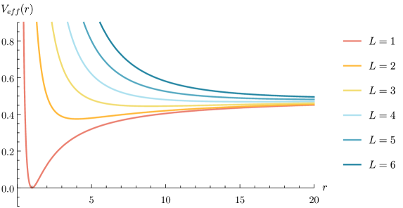
Figure 2: Shape of the effective potential $V_{e\!f\!f}$ as a function of the coordinate radius, for massive particles in Newtonian gravity. Colored curves refer to different values of $L$ (we scale lengths such that $M=1$). As the angular momentum increases, the radius $r_{*}$ corresponding to the the minimum of the potential also increases, and so does the value of the potential $V_{e\!f\!f}(r_{*})$. Note that the potential tends to $1/2$ as $L\to+\infty$.

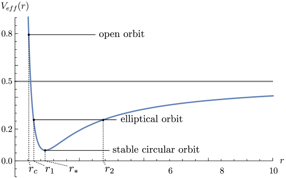
Figure 3: Effective potential $V_{e\!f\!f}$ (blue curve) as a function of the radial coordinate $r$ for massive particles in Newtonian gravity, assuming $L=1.07$ ($M=1$). For large values of $r$, the effective potential approaches the asymptotic limit $V_{eff}\rightarrow\frac{1}{2}$ (gray horizontal line). We show as black lines three possible cases for the energy $\mathcal{E}$: (i) if the energy matches the minimum of the potential, the particle remains in a stable circular orbit with radius $r_{*}$; (ii) if $\mathcal{E}$ falls between the asymptotic limit and the minimum, the orbit becomes elliptical, with the radius oscillating between $r_{1}$ and $r_{2}$; (iii) for energies higher than the asymptotic value, the particle approaches the source up to a minimum radius $r_{c}$ and then moves on an open orbit.

Massive particles in General Relativity.

The effective potential for massive particles in GR involves all four terms in Eq. (51). For $\gamma=1$, the behavior depends on the choice of the angular momentum, as shown in Fig. 4. For $L^{2}<12M^{2}$, the potential only has imaginary roots, i.e., no extreme points, and the orbits is forced to move towards the source. When $L^{2}>12M^{2}$, the two roots in Eq. (54) become real, corresponding to a maximum and a minimum. The former identifies unstable circular orbits, with a radius $3M\leq r_{-}<6M$. Stable circular orbits are possible in correspondence of the minimum, with a radius $r_{+}\geq 6M$. In GR, massive particles can exist on stable circular orbits up to $6M$, while inner circular orbits, up to $3M$, are inherently unstable. The critical radius marking the onset of stable trajectories, $r_{\text{ISCO}}=6M$, is known as the Innermost Stable Circular Orbit. In Figs. 5-7 we show different possible configurations for the effective potential, and for different types of orbits. Depending on the value of the particle energy, the body can follow circular elliptical, radially bound or unbounded trajectories [20].

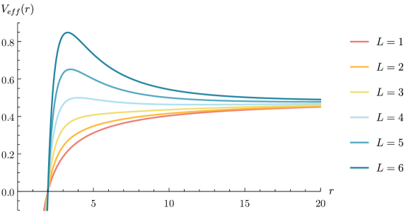
Figure 4: Effective potential for massive particles in General Relativity, $V_{e\!f\!f}(r)$, for different values of the angular momentum $L$ ($M=1$). When $L^{2}<12M^{2}$ there are no extreme points. At $L^{2}=12M^{2}$, a single extremum (a saddle point) emerges. As $L$ increases, two extrema appear, a minimum $r_{+}$ and a maximum $r_{-}$, which gets more separated when $L$ grows. For $12M^{2}<L^{2}\leq 16M^{2}$, the effective potential at the maximum $V_{e\!f\!f}(r_{-})$ remains smaller or equal to the asymptotic limit, while it exceeds the latter for $L^{2}>16M^{2}$.

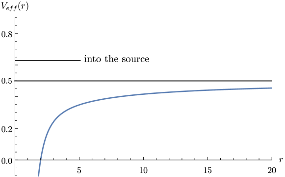
Figure 5: Effective potential for massive particles in General Relativity as a function of the coordinate radius $r$, for $L=1.07$ (with $M=1$). In this case, there are no extrema.

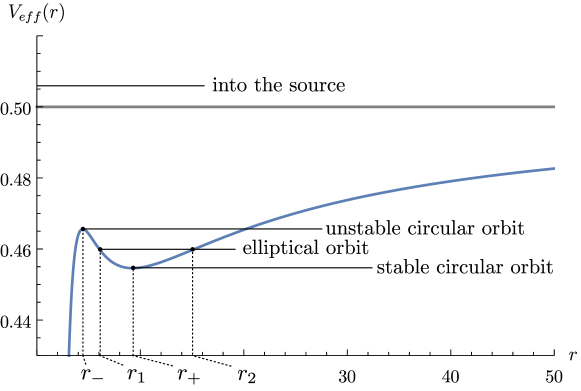
Figure 6: Same as Fig. 5 but for $L=3.7$. Horizontal lines identify massive particles with different energy states. Here, the potential shows both a minimum $r_{+}$ and a maximum $r_{-}$, which correspond to a stable and unstable circular orbit, respectively. Elliptical orbits take place between $r_{1}$ and $r_{2}$.

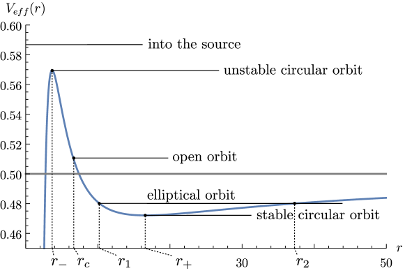
Figure 7: Same as Fig. 6 but assuming for the angular momentum of the massive particle $L=4.5$. Note that, unlike the configuration shown in Fig. 6, the maximum of the potential is above the the asymptotic value, allowing for open orbits.

3.3 Orbits of massless particles

For massive particles, i.e., $\epsilon=0$, the effective potential (51) reads

$$V_{e\!f\!f}(r)=\frac{L^{2}}{2r^{2}}-\gamma\frac{ML^{2}}{r^{3}}\ .$$ (55)

The asymptotic value of the potential for $r\to+\infty$ is the same in the relativistic and in the Newtonian model, and tends to zero. When $r\to 0^{+}$, the behaviour is the same as described in Eq. (53).

Massless particles in Newtonian gravity.

When $\gamma=0$, the effective potential reduces to $V_{e\!f\!f}(r)=\frac{L^{2}}{2r^{2}}$, which has no roots. Hence, for non-zero values of the angular momentum $L$ massless particles hit the potential at some distance from the source, moving away from it. In NG massless particles cannot stay on bound orbits around the source, and only unbounded trajectories are allowed (see Figs. 8 and 9).

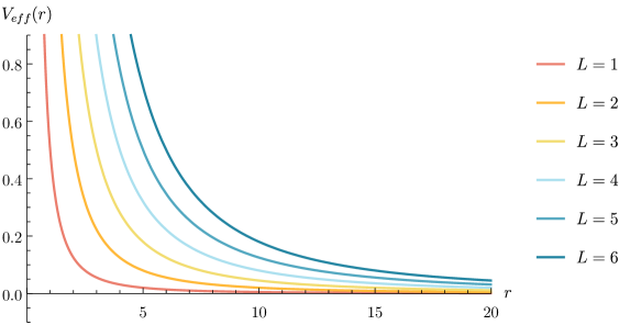
Figure 8: Effective potential for massless particles in Newtonian gravity as a function of $r$. In this case there are no extrema.

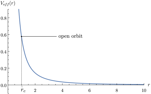
Figure 9: Same as Fig. 8 for a particular choice of the angular momentum $L=1.07$. In this configuration only open orbits are possible, featuring a minimum distance $r_{c}$.

Massless particles in General Relativity.

In this case, the effective potential (55) yields a single root, $\bar{r}=3M$, which corresponds to a maximum. This result holds for every non-zero value of $L$, as shown in Fig. 10 and Fig. 11. At variance with the NG case, the relativistic description highlights three possible scenarios depending on the energy $\mathcal{E}$. Particles can indeed follow open orbits when $\mathcal{E}<V_{e\!f\!f}(\bar{r})$. If $\mathcal{E}=V_{e\!f\!f}(\bar{r})$, the particle remains on a circular orbit, although unstable. For $\mathcal{E}>V_{e\!f\!f}(\bar{r})$ the particle falls into the source.

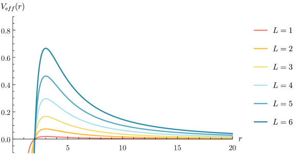
Figure 10: Effective potential for massless particles in General Relativity as a function of the radial distance $r$ and of the angular momentum $L$ (with $M=1$). The maximum of $V_{e\!f\!f}$ decreases for smaller values of $L$.

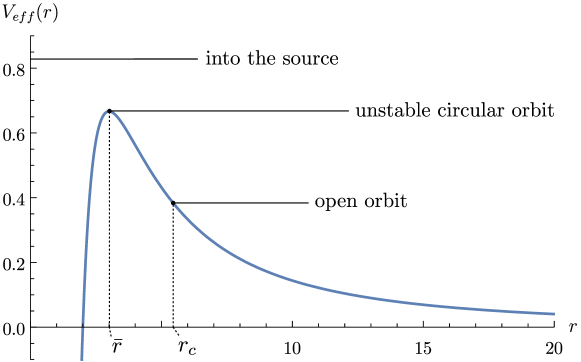
Figure 11: Same as Fig. 10, but assuming $L=6$.

4 Schwarzschild black holes

In Sec. 2, we concluded our discussion on the nature of the singularities for the Schwarzschild metric, finding that $R_{S}=2M$ is a coordinate singularity, while $r=0$ remains a true, physical one. In this section, we want to study more in detail the spacetime region around $R_{S}$, adopting a suitable choice of coordinates.

Let us consider lightlike geodesics that are radial ($\theta$ and $\phi$ both constant) within the Schwarzschild metric (23):

$$ds^{2}=-\left(1-\frac{R_{S}}{r}\right)dt^{2}+\left(1-\frac{R_{S}}{r}\right)^{-1}dr^{2}=0\ ,$$ (56)

hence the slope of the light cones in a $t$-$r$ diagram is

$$\frac{dt}{dr}=\pm\left(1-\frac{R_{S}}{r}\right)^{-1}\ .$$ (57)

At large distances from the source, $r\to+\infty$, the slope tends to $\pm 1$, as expected for a flat metric, since the Schwarzschild solution is asymptotically flat. On the other side of the domain, as we reach the Schwarzschild radius, $r\to R_{S}$, the slope diverges, $\frac{dt}{dr}\to\pm\infty$. This implies that as we move towards $R_{S}$ the slope of the light cone increases such that it becomes progressively narrower (see the sketch in Fig. 12). Hence, an infalling particle will appear to slow down as it approaches $R_{S}$ from the perspective of external observers using Schwarzschild coordinates. In other words, we will perceive a particle taking an infinite amount of time to reach the Schwarzschild radius. However such problematic description is rooted in our choice of coordinates, and an alternative system is needed.

Figure 12: Graphical representation in the $t$-$r$ plane of light cones in the Schwarzschild metric, shrinking as $r=R_{S}$ is approached.

4.1 The tortoise coordinate

A common choice involves shifting the Schwarzschild surface to $-\infty$ by adopting a different coordinate time that varies more slowly as we approach $R_{S}$. To achieve this, we introduce the so-called tortoise coordinate:

$$r^{*}=r+2M\log\left(\frac{r}{2M}-1\right)\ ,$$ (58)

which allows to rewrite the Schwarzschild metric such that the line element (23) reads

$$ds^{2}=\left(1-\frac{2M}{r}\right)\left(-dt^{2}+dr^{*}{}^{2}\right)+r^{2}d\Omega^{2}\ ,$$ (59)

where $r=r(r^{*})$. The metric in these coordinates remains well-behaved at $R_{S}=2M$. Solving Eq. (57), we find $t=\pm r^{*}+c$, where $c$ is an integration constant. The plus and minus signs correspond to outgoing and ingoing massless geodesics, respectively. The behavior of light cones in the $t$-$r$ and $t$-$r^{*}$ diagrams is illustrated in Fig. 13, showing the difference in the choice of radial coordinate $r$ and the tortoise coordinate $r^{*}$.

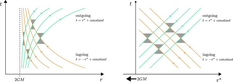
Figure 13: Massless ingoing (green) and outgoing (orange) geodesics of the Schwarzschild metric. (Left) Light cones (in gray) deform as $r=R_{S}$ is approached when using the Schwarzschild radial coordinate $r$. (Right) When using the tortoise radial coordinate $r^{*}$, the Schwarzschild radius is pushed to minus infinity, and the light cones remain undeformed.

4.2 Eddington–Finkelstein coordinates

We can use coordinates adapted to ingoing or outgoing massless particles, obtained as follows:

$$v=t+r^{*}\ ,\qquad u=t-r^{*}\ .$$ (60)

An ingoing lightlike particle is indeed characterized by $v=constant$, while an outgoing particle by $u=constant$. Using the Schwarzschild radial coordinate $r$, with either $v$ or $u$ as the coordinate time, we have the ingoing Eddington–Finkelstein (EF) coordinates or the outgoing Eddington–Finkelstein coordinates, respectively. In these coordinate systems, the Schwarzschild metric is given by

ingoing EF $$ds^{2}=-\left(1-\frac{2M}{r}\right)dv^{2}+2dvdr+r^{2}d\Omega^{2}\ ,$$ (61)

outgoing EF $$ds^{2}=-\left(1-\frac{2M}{r}\right)du^{2}-2dudr+r^{2}d\Omega^{2}\ .$$

The metric shown in (61) is explicitly nonsingular, invertible, and its inverse does not have any divergent component.

If we consider a lightlike radial geodesic in these coordinates, we can compute the slope of the light cones in a $v$-$r$ or $u$-$r$ diagram:

$$\frac{dv}{dr}=\begin{cases}0\ ,\\ 2\left(1-\frac{2M}{r}\right)^{-1}\ ,\end{cases}\qquad\frac{du}{dr}=\begin{cases}-2\left(1-\frac{2M}{r}\right)^{-1}\ ,&\qquad\text{ingoing}\ ,\\ 0\ .&\qquad\text{outgoing}\ .\end{cases}$$ (62)

In the ingoing EF coordinates, ingoing geodesics are straight lines, while outgoing geodesics are divided into two separate families, depending on whether $r<R_{S}$ or $r>R_{S}$, as shown in Fig. 14. As we move towards the Schwarzschild radius, the light cones tilt more and more, until the future light cone is completely inside $R_{S}$.

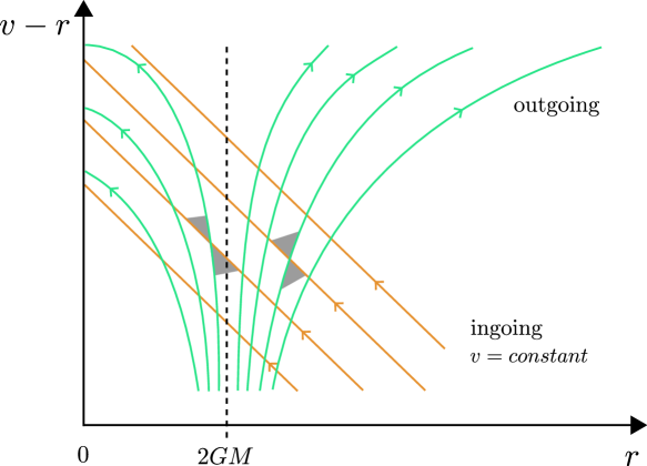
Figure 14: Massless ingoing (green) and outgoing (orange) geodesics of the Schwarzschild metric in the ingoing EF coordinates. Light cones (in gray) tilt more and more as the Schwarzschild radius is approached.

This reflects an important feature of the surface at $r=R_{S}=2M$, the event horizon, which is a no-return region. A particle in the direction of the singularity $r=0$, which crosses $R_{S}$, cannot escape and is destined to fall into the source. The event horizon divides the spacetime into two causally disconnected domains: an outside observer can send signals both inward and outward, but can not know what happens inside the horizon.

5 Perturbations of Schwarzschild black holes

Before entering into the details of relativistic perturbations of the Schwarzschild spacetime, it is instructive to discuss a scattering toy model, that encodes many properties common to the more intricate scenario we treat afterwards.

5.1 A scattering toy problem

Let us consider a scattering problem defined by the following second-order differential equation:

$$\left[\frac{d^{2}}{dx^{2}}+\omega^{2}-2V_{0}\delta(x)\right]\psi(\omega,x)=i\omega\,\psi_{0}(x)\ ,$$ (63)

where $x\in(-\infty,\infty)$. Equation (63) features a localized effective potential and a source term related to the initial configuration. For simplicity, we also assume that the latter is localized, namely, $\psi_{0}(x)=\psi(t=0,x)=\delta(x-x_{0})$. A general solution to the family of problems in Eq. (63) involves first solving the associated homogeneous equation and then constructing the full solution considering the source term [21]. The homogeneous problem yields two solutions, identifying growing and decaying modes on both sides of the delta function. In particular, by requiring a purely ingoing wave as $x\rightarrow-\infty$, the solution propagating as $x\rightarrow\infty$ is the sum of outgoing and ingoing modes:

$$\psi_{\textnormal{L}}=\begin{cases}e^{-i\omega x}\ ,&x\rightarrow-\infty\ ,\\ A_{\textnormal{in}}e^{-i\omega x}+A_{\textnormal{out}}e^{i\omega x}\ ,&x\rightarrow+\infty\ .\end{cases}$$ (64)

Requiring continuity of the solution at $x=0$ leads to $A_{\textnormal{in}}+A_{\textnormal{out}}=1$. Using the field equation to compute the jump of the first derivative, we integrate the master equation (63) within $[-\epsilon,\epsilon]$ as $\epsilon\rightarrow 0$:

$$\int_{-\epsilon}^{+\epsilon}\!dx\,\frac{d^{2}}{dx^{2}}\psi_{\textnormal{L}}+\int_{-\epsilon}^{+\epsilon}\!dx\,\omega^{2}\psi_{\textnormal{L}}=\int_{-\epsilon}^{+\epsilon}\!dx\,2V_{0}\,\delta(x)\,\psi_{\textnormal{L}}\ .$$ (65)

The second integral of the left-hand side vanishes assuming that $\psi_{\textnormal{L}}(x)$ is continuous. Hence, we have

$$\frac{d\psi_{\textnormal{L}}}{dx}\bigg{|}_{-\epsilon}^{+\epsilon}=2V_{0}\,\psi_{\textnormal{L}}(x=0)\ .$$ (66)

Combining the former with the condition on the wave amplitude we obtain

$$\begin{cases}A_{\textnormal{in}}+A_{\textnormal{out}}=1\ ,\\ -i\omega A_{\textnormal{in}}+i\omega A_{\textnormal{out}}+i\omega=2V_{0}\ ,\end{cases}$$ (67)

hence

$$A_{\textnormal{in}}=1+\frac{iV_{0}}{\omega}\ ,\qquad A_{\textnormal{out}}=-\frac{iV_{0}}{\omega}\ .$$ (68)

Let us now compute the Wronskian between $\psi_{\textnormal{L}}(x)$ and a second solution, labelled $\psi_{\textnormal{R}}(x)$, which behaves as purely outgoing at infinity, i.e., $\psi_{\textnormal{R}}(x)=e^{i\omega x}$ as $x\rightarrow\infty$:

$$W =\frac{d\psi_{\textnormal{R}}}{dx}\psi_{\textnormal{L}}-\frac{d\psi_{\textnormal{L}}}{dx}\psi_{\textnormal{R}}$$ (69)

$$=i\omega e^{i\omega x}(A_{\textnormal{out}}e^{i\omega x}+A_{\textnormal{in}}e^{-i\omega x})-e^{i\omega x}(i\omega A_{\textnormal{out}}e^{i\omega x}-i\omega A_{\textnormal{in}}e^{-i\omega x})$$

$$=i\omega A_{\textnormal{out}}e^{2i\omega x}+i\omega A_{\textnormal{in}}-i\omega A_{\textnormal{out}}e^{2i\omega x}+i\omega A_{\textnormal{in}}=2i\omega A_{\textnormal{in}}\ .$$

Replacing the value of $A_{\textnormal{in}}$ found before (see Eq. (68)), we obtain an analytic expression of the Wronskian:

$$W=2i\omega A_{\textnormal{in}}=2i\omega+2i^{2}V_{0}=2i\omega-2V_{0}\ .$$ (70)

The two solutions $\psi_{\textnormal{L,R}}(x)$ are linearly dependent if the values of $\omega$ solve the eigenvalue problem given by the second order equation (63), i.e., if they correspond to the QNMs of the system. In this case $W=0$, or equivalently $\omega=-iV_{0}$.

We can now focus on the inhomogeneous problem. We first find the general solution in Fourier space using a Green-function approach:

$$\psi(\omega,x)=\psi_{\textnormal{R}}\int_{-\infty}^{x}\!dx\,\frac{I\,\psi_{\textnormal{L}}}{W}+\psi_{\textnormal{L}}\int^{\infty}_{x}\!dx\,\frac{I\,\psi_{\textnormal{R}}}{W}\ ,$$ (71)

where $I=i\omega\,\psi_{0}(x)$. For $x\gg 1$, we can write the previous solution as

$$\psi(\omega,x) =\psi_{\textnormal{R}}\int_{-\infty}^{\infty}\!dx\,\frac{I\,\psi_{\textnormal{L}}}{W}$$ (72)

$$=\psi_{\textnormal{R}}\int_{-\infty}^{\infty}\!dx\,i\omega\frac{\psi_{\textnormal{L}}}{W}\delta(x-x_{0})$$

$$\simeq\frac{i\omega}{W}e^{i\omega x}\left[A_{\textnormal{in}}e^{-i\omega x_{0}}+A_{\textnormal{out}}e^{i\omega x_{0}}\right]\,,\qquad x_{0}>0\ .$$

Replacing the value of $W$ in terms of $A_{\textnormal{in}}$, the we finally obtain

$$\psi(\omega,x)=\frac{1}{2}e^{i\omega(x-x_{0})}+\frac{1}{2}e^{i\omega(x+x_{0})}\frac{A_{\textnormal{out}}}{A_{\textnormal{in}}}\ .$$ (73)

We can invert the solution to find the its expression in the time domain:

$$\psi(t,x) =\frac{1}{2\pi}\int_{-\infty}^{\infty}\!dx\,e^{-i\omega t}\psi(\omega,x)$$ (74)

$$=\frac{1}{4\pi}\int_{-\infty}^{\infty}\!d\omega\,e^{i\omega[(x-x_{0})-t]}+\frac{1}{4\pi}\int_{-\infty}^{\infty}\!d\omega\,\frac{A_{\textnormal{out}}}{A_{\textnormal{in}}}e^{i\omega[(x+x_{0})-t]}\ ,$$

and, using the definition of the delta function,

$$\psi(t,x)=\frac{1}{2}\delta(x-x_{0}-t)+\frac{1}{2\pi}\int_{-\infty}^{\infty}\!d\omega\,\frac{-iV_{0}}{\omega+iV_{0}}e^{i\omega[(x+x_{0})-t]}\ .$$ (75)

The second integral has a pole at $\omega=-V_{0}$, corresponding to the QNM frequencies. This integral can be solved using contour integrals by extending the domain into the complex plane and applying the residue theorem. There are two cases to consider.

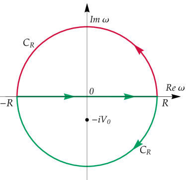
Figure 15: Contour path used to perform the integral in Eq. (75). The pole corresponding to the QNM, $-iV_{0}$, is located in the negative imaginary panel.

For $x+x_{0}-t>0$ $(t<x+x_{0})$, we close the path in the upper panel. The integral vanishes as there are no poles inside the contour. Conversely, for $x+x_{0}-t<0$ $(t>x+x_{0})$, we close the path in the bottom panel. In this case, the integral over the path shown in Fig. 15 reads:

$$\ointclockwise_{\gamma}\!d\omega\,f(\omega)e^{i\omega[x+x_{0}-t]} =\int_{C_{R}}\!d\omega\,f(\omega)e^{i\omega[x+x_{0}-t]}+\int_{-R}^{R}\!d\omega\,f(\omega)e^{i\omega[x+x_{0}-t]}$$ (76)

$$=2\pi i\lim_{\omega\rightarrow-iV_{0}}\left[(\omega+iV_{0})f(\omega)e^{i\omega[x+x_{0}-t]}\right]$$

$$=\frac{V_{0}}{2}e^{V_{0}(x+x_{0}-t)}\ ,$$

where $2\pi f(\omega)=-iV_{0}/(\omega+iV_{0})$. In summary, we obtain the following full solution:

$$\begin{cases}\psi(t,x)=\frac{1}{2}\delta(x-x_{0}-t)\ ,&t<x+x_{0}\ ,\\ \psi(t,x)=\frac{1}{2}\delta(x-x_{0}-t)+\frac{V_{0}}{2}e^{V_{0}(x+x_{0}-t)}\ ,&t>x+x_{0}\ .\end{cases}$$ (77)

These equations provide a clear picture of the response of the system under a given perturbation, which can classified into two regimes. At early times ($t<x+x_{0}$), we have a prompt response or a direct signal: the radiation propagates towards the observer without having the time to interact with the potential barrier and return. Later, for $t>x+x_{0}$, we also appreciate the effect due to the QNM. The radiation interacts with the potential barrier, and within a time $x-x_{0}+2x_{0}=x+x_{0}$, the observer see the trains of modes.

Figure 16: Schematic representation of the barrier-observer setup for the scattering problem defined by equation (63).

The picture describing the black hole response to an external perturbation remains qualitatively the same. Instead of the delta function, the scattering will be characterized by an effective potential. The time-domain response will exhibit a prompt effect originating from the initial data, while the other contribution will be absorbed by the black hole and excite its modes. After a certain interval of time, this excitation leads to the ringdown signal. Notably, the excitation of the QNMs is localized at a very special place: the light ring.

5.2 Scalar field perturbations

Instead of going through all the steps to compute gravitational perturbations of the Schwarzschild metric, let us focus on the perturbations induced by a massive scalar field on the background spacetime. As we will discuss at the end of this section, the results obtained for this probe field are generic enough to be straightforwardly generalized to vector and tensor perturbations, without the need for a more complicated mathematical formalism.

We consider a scalar field $\phi$ that is minimally coupled with gravity, described by the following action:

$$S=S_{\textnormal{EH}}+S_{\phi}=\int\!d^{4}x\,\sqrt{-g}\,\gamma\,R+\int\!d^{4}x\,\sqrt{-g}\left(\kappa\,\partial_{\mu}\phi\,\partial^{\mu}\phi+\beta\,\phi^{2}\right)\ .$$ (78)

Here, $S_{\textnormal{EH}}$ and $S_{\phi}$ identify the Einstein–Hilbert and the scalar field actions, respectively, with $\gamma$, $\kappa$, and $\beta$ being three coupling constants. The equations of motion can be derived from the action using the Euler–Lagrange equations [22]

$$\frac{\partial\mathcal{L}}{\partial\psi}-\nabla_{\mu}\left(\frac{\partial\mathcal{L}}{\partial\partial_{\mu}\psi}\right)=0\ ,$$ (79)

where $\nabla_{\mu}$ represents the covariant derivative, (also denoted hereafter by a semicolon), and $\mathcal{L}(\psi,\nabla\psi)$ is the Lagrangian density of the system, a function of the fields $\psi$ and their derivatives. The Euler–Lagrange equations for the scalar field yield

$$\frac{\partial\mathcal{L}_{\phi}}{\partial\phi}=2\sqrt{-g}\,\beta\,\phi\ ,\qquad\frac{\partial\mathcal{L}}{\partial\partial_{\mu}\phi}=2\sqrt{-g}\,\kappa\,\partial^{\mu}\phi\ ,$$ (80)

which leads to

$$2\sqrt{-g}\left(\beta\,\phi-\kappa\,\nabla_{\mu}\partial^{\mu}\phi\right)=2\sqrt{-g}\left(\beta\,\phi-\kappa\,\Box\phi\right)=0\ .$$ (81)

Choosing $\kappa=1$ and $\beta=\mu^{2}$ leads to the well-known Klein–Gordon equation for a scalar field with mass $\mu$

$$(\Box-\mu^{2})\phi=\frac{1}{\sqrt{-g}}\partial_{\mu}\left(\sqrt{-g}\,\partial^{\mu}\phi\right)-\mu^{2}\phi=0\ .$$ (82)

The second equality can be derived from the following identity:

$$\tensor{V}{{}^{\mu}_{;\mu}}=\frac{1}{\sqrt{-g}}\left(\sqrt{-g}\,V^{\mu}\right)_{,\mu}\ ,$$ (83)

when applied to the d’Alambert operator $\Box=\nabla_{\mu}\nabla^{\mu}$ acting on a scalar field. Variation of the $S_{\textnormal{EH}}$ with respect to the metric yields the canonical Einstein Tensor, while from the scalar field Lagrangian

$$\frac{\partial\mathcal{L}_{\phi}}{\partial g^{\mu\nu}}=-\frac{1}{2}g_{\mu\nu}\mathcal{L}_{\phi}+\sqrt{-g}\kappa\nabla_{\mu}\phi\nabla_{\nu}\phi\ ,\quad\frac{\partial\mathcal{L}_{\phi}}{\partial\partial_{\sigma}\tensor{g}{{}^{\mu}{}^{\nu}}}=0\ ,$$ (84)

leading to

$$R_{\mu\nu}-\frac{1}{2}g_{\mu\nu}R=\gamma^{-1}\,T_{\mu\nu}\ ,\qquad T_{\mu\nu}=\frac{1}{2}g_{\mu\nu}\left(\kappa\,\partial_{\alpha}\phi\partial^{\alpha}\phi+\beta\,\phi^{2}\right)-\kappa\partial_{\mu}\phi\partial_{\nu}\phi\ ,$$ (85)

where $T_{\mu\nu}$ is the effective stress-energy tensor introduced by scalar field. We have obtained, therefore, a set of coupled equations of motion for the scalar field (81) and the gravitational field (85).

Here, we assume that $\phi$ provides a small perturbation of the background spacetime and consider only linear-order terms in the scalar field. We can neglect quadratic contributions coming from $T_{\mu\nu}$, such that the metric and the scalar sector decouple. In this framework, the scalar field does not backreact on the metric, evolving on a fixed background given as a solution of the Einstein equations in vacuum.

5.3 The master equation

To keep our discussion as general as possible, we consider here a static and spherically symmetric spacetime defined by Eq. (10), in which we have relabeled $e^{2\alpha}$ and $e^{2\beta}$ as $A$ and $B^{-1}$, respectively, such that the line element reads

$$ds^{2}=-A(r)dt^{2}+B^{-1}(r)dr^{2}+r^{2}d\Omega^{2}\ .$$ (86)

We can exploit the symmetries of the background and assume that the evolution of $\phi(t,r,\theta,\varphi)$ is independent of rotation, decoupling the angular variables $\theta$, $\varphi$ from $t$, $r$. Hence, we decompose the scalar field into spherical harmonics $Y_{\ell m}(\theta,\varphi)$:

$$\phi(t,r,\theta,\varphi)=\sum\limits_{\ell=0}^{\infty}\sum_{m=-\ell}^{\ell}\frac{\psi_{\ell m}(r)}{r}e^{-i\omega t}Y_{\ell m}(\theta,\varphi)\ ,\qquad Y_{\ell m}(\theta,\varphi)=N\,e^{im\varphi}P_{\ell m}(\theta)\ ,$$ (87)

where $P_{\ell m}(\theta)$ are the Legendre polynomials of the second kind, $N$ is a normalization factor, and we have factored out the time dependence of the perturbation, leaving the radial function $\psi_{\ell m}(r)$. We replace Eqs. (86) and (87) into the Klein–Gordon equation (82), to find a master equation for $\psi_{\ell m}(r)$. First, the term within round brackets in the right-hand side of Eq. (82) becomes

$$\sqrt{-g}\,\partial^{\mu}\phi =\sqrt{-g}\,g^{\mu\nu}\partial_{\nu}\phi$$ (88)

$$=\sqrt{\frac{A}{B}}\,r^{2}\sin\theta\left(-A^{-1}\delta^{\mu}_{t}\partial_{t}+B\delta^{\mu}_{r}\partial_{r}+r^{-2}\delta^{\mu}_{\theta}\partial_{\theta}+r^{-2}\sin^{-2}\theta\,\delta^{\mu}_{\varphi}\partial_{\varphi}\right)\phi\ ,$$

where $g^{\mu\nu}=\operatorname{diag}(-A^{-1},B,r^{-2},r^{-2}\sin^{-2}\theta)$, and $\sqrt{-g}=\sqrt{A/B}r^{2}\sin\theta$. The partial derivatives of the scalar field expanded in spherical harmonics read

$$\partial_{t}\phi=-i\omega\,\phi\quad\ , \quad\partial_{r}\phi=\sum_{\ell m}\frac{e^{-i\omega t}Y_{\ell m}}{r^{2}}(r\psi^{\prime}_{\ell m}-\psi_{\ell m})\ ,$$ (89)

$$\partial_{\theta}\phi=\sum_{\ell m}\frac{e^{-i\omega t}\psi_{\ell m}}{r}\,\partial_{\theta}Y_{\ell m}\quad\ , \quad\partial_{\varphi}\phi=\sum_{\ell m}\frac{e^{-i\omega t}\psi_{\ell m}}{r}\,\partial_{\varphi}Y_{\ell m}\ ,$$ (90)

where a prime denotes the derivative with respect to the radial coordinate $r$. Next, we compute the full expression for $\partial_{\mu}\left(\sqrt{-g}\,\partial^{\mu}\phi\right)$:

$$\partial_{\mu}\left(\sqrt{-g}\,\partial^{\mu}\phi\right) =\sqrt{-g}\,e^{-i\omega t}\sum_{\ell m}\left[\tfrac{\omega^{2}}{A}\tfrac{\psi_{\ell m}}{r}+B\left(-\tfrac{A^{\prime}}{2A}\tfrac{\psi_{\ell m}}{r^{2}}+\tfrac{A^{\prime}}{2A}\tfrac{\psi^{\prime}_{\ell m}}{r}+\tfrac{\psi_{\ell m}^{\prime\prime}}{r}\right)+B^{\prime}\left(-\tfrac{\psi_{\ell m}}{2r^{2}}+\tfrac{\psi_{\ell m}^{\prime}}{2r}\right)\right.$$ (91)

$$\qquad\left.+\tfrac{\psi_{\ell m}}{r^{3}}\left(\csc^{2}\theta\,\partial^{2}_{\varphi}+\cot\theta\,\partial_{\theta}+\partial^{2}_{\theta}\right)\right]Y_{\ell m}\ .$$

Note that the previous equation can be greatly simplified by exploiting the properties of the spherical harmonics and their derivatives:

$$\partial^{2}_{\phi}Y_{\ell m}(\theta,\varphi) =-m^{2}N\,e^{im\varphi}P_{\ell m}(\theta)=-m^{2}Y_{\ell m}(\theta,\varphi)\ ,$$ (92)

$$\partial_{\theta}Y_{\ell m}(\theta,\varphi) =N\,e^{im\varphi}\partial_{\theta}P_{\ell m}(\theta)\ ,$$

and the same for the second derivative with respect to $\theta$. We can now use the following identity of the Legendre polynomials:

$$\csc\theta\,\partial_{\theta}\left(\sin\theta\,\partial_{\theta}P_{\ell m}\right)-m^{2}\csc^{2}\theta P_{\ell m}=-\ell(\ell+1)P_{\ell m}\ ,$$ (93)

hence

$$\left(\cot\theta\,\partial_{\theta}+\partial^{2}_{\theta}\right)P_{\ell m}=\left(-\ell(\ell+1)+m^{2}\csc^{2}\theta\right)P_{\ell m}\ .$$ (94)

Therefore, the terms between parentheses in the second line of Eq. (91) can be recast simply as

$$\left(\csc^{2}\theta\,\partial^{2}_{\varphi}+\cot\theta\,\partial_{\theta}+\partial^{2}_{\theta}\right)Y_{\ell m}=-\ell(\ell+1)Y_{\ell m}\ .$$ (95)

We can therefore rewrite the Klein–Gordon equation (82) as

$$e^{-i\omega t}\sum_{\ell m}\left[\tfrac{\omega^{2}}{A}\tfrac{\psi_{\ell m}}{r}+B\!\left(-\tfrac{A^{\prime}}{2A}\tfrac{\psi_{\ell m}}{r^{2}}+\tfrac{A^{\prime}}{2A}\tfrac{\psi^{\prime}_{\ell m}}{r}+\tfrac{\psi_{\ell m}^{\prime\prime}}{r}\right)+B^{\prime}\!\!\left(-\tfrac{\psi_{\ell m}}{2r^{2}}+\tfrac{\psi_{\ell m}^{\prime}}{2r}\right)-\tfrac{\psi_{\ell m}}{r^{3}}\ell(\ell+1)\right]\!Y_{\ell m}=0\ ,$$ (96)

and, after further simplifications,

$$AB\frac{d^{2}\psi_{\ell m}}{dr^{2}}+\frac{(AB)^{\prime}}{2}\frac{d\psi_{\ell m}}{dr}+\left(\omega^{2}-\mu^{2}A-\frac{\ell(\ell+1)}{r^{2}}A-\frac{(AB)^{\prime}}{2r}\right)\psi_{\ell m}=0\ ,$$ (97)

where we have made the sum over the multipolar indices $(\ell,m)$ implicit. We introduce now the generalized tortoise coordinate $r^{*}$, defined by

$$dr^{*}{}^{2}=(AB)^{-1}dr^{2}\ ,$$ (98)

which reproduces the well-known Schwarzschild tortoise coordinate (58) for $A=B=1-R_{S}/r$. By this change, the master equation (97) takes the particularly simple form

$$\frac{d^{2}\psi_{\ell m}(r)}{dr^{*}{}^{2}}+\left[\omega^{2}-V(r)\right]\psi_{\ell m}(r)=0\ ,\quad V(r)=\mu^{2}A+\frac{\ell(\ell+1)}{r^{2}}A+\frac{(AB)^{\prime}}{2r}\ .$$ (99)

The calculations carried out so far show that the scalar field perturbations in a fixed, spherically-symmetric background are controlled by a single master equation (99), which involves only the radial component of the perturbation, $\psi_{\ell m}(r)$, and resembles the Schrödinger equation with a scattering potential $V(r).$ This analogy allows for quick physical insights into the general features of the scattering process and enables the utilization of various resolution techniques developed in the context of quantum mechanics [23].

5.4 Properties of the master equation

We can now proceed by assuming the Schwarzschild metric, such that the scattering potential in Eq. (99) reads

$$V(r)=\left(1-\frac{2M}{r}\right)\left(\mu^{2}+\frac{\ell(\ell+1)}{r^{2}}+\frac{2M}{r^{3}}\right)\ .$$ (100)

For a given scalar field mass $\mu$ and multipole $\ell$, the potential is function of the radial coordinate and: (i) it vanishes at spatial infinity, $r\rightarrow\infty$, (ii) it tends to $\mu^{2}$ as $r\rightarrow 2M$ (or $r^{*}\rightarrow-\infty)$. Figure 17 shows the behavior of $V(r)$ for various values of $\mu$ and $\ell$. Hereafter we will analyze different properties of $V(r)$ and the master equation to introduce the QNMs frequencies of a Schwarzschild BH. For now on we will focus on the massless case $\mu=0$.

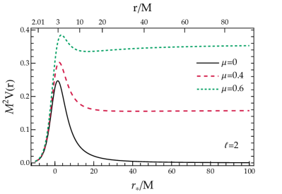
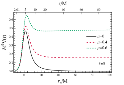
Figure 17: Scattering potential of the master equation (99) for a Schwarzschild background, with $\ell=2$ (left) and $\ell=3$ (right). Colored curves correspond to different values of the scalar mass $\mu$. The top and bottom axes represent values of the Schwarzschild coordinate radius $r$ and the tortoise coordinate $r^{*}$, respectively.

The peak of the scattering potential.

Examining the two panels in Fig. 17, we observe that the peak of the scattering potential is located suspiciously close to $r=3M$, regardless of the values of $\ell$. To further investigate this feature, we study the extrema of the scattering potential

$$V(r)=\left(1-\frac{2M}{r}\right)\left(\frac{\ell(\ell+1)}{r^{2}}+\frac{2M}{r^{3}}\right)\ .$$ (101)

The critical points of $\omega^{2}-V(r)$ are given by the roots of

$$V^{\prime}(r)=-\frac{4R_{S}^{2}}{r^{5}}-\frac{3R_{S}[\ell(\ell+1)-1]}{r^{4}}+\frac{2\ell(\ell+1)}{r^{3}}\ ,$$ (102)

which can be found analytically, and read

$$r_{\pm}=\frac{M}{2\ell(\ell+1)}\left[3(\ell(\ell+1)-1)\pm\sqrt{9+\ell(\ell+1)(14+9\ell(\ell+1))}\right]\ .$$ (103)

The physical solutions, which provide positive radii, are given by $r_{+}$. Interestingly, as $\ell\to+\infty$, in the so called eikonal limit, $r_{+}$ tends to $3M$, as shown in Fig. 18. In Sec. 3.3, we have seen that $r=3M$ has a special meaning for the Schwarzschild spacetime, as it corresponds to the location of the unstable circular orbit for massless particles. This analysis demonstrates the remarkable correspondence between the maximum of the scattering potential and the photon ring [23].

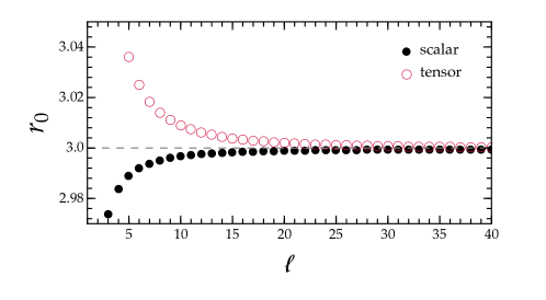
Figure 18: Location of the peak of the scattering potential (101) as a function of $\ell$, for scalar and tensor perturbations.

General master equation.

Thus far, we have focused on the perturbations of a test scalar field on a fixed Schwarzschild BH, finding that they reduce to the single equation (99). We could follow similar steps to compute vector and tensor perturbations, studying the metric response. Surprisingly, while the calculations would become more complicated and require different mathematical techniques, they would lead to results extremely close to Eq. (99). We can introduce a generalized master equation:

$$\begin{gathered}\frac{d^{2}\psi_{\ell m}(r)}{dr^{*}{}^{2}}+\left[\omega^{2}-V_{s}(r)\right]\psi_{\ell m}(r)=0\ ,\qquad\\ V_{s}(r)=\left(1-\frac{2M}{r}\right)\left[\frac{\ell(\ell+1)}{r^{2}}+\frac{2M(1-s^{2})}{r^{3}}\right]\ ,\end{gathered}$$ (104)

where the parameter $s$ identifies the type of perturbation, taking values $s=0,1,2$ for scalar, vector, and tensor modes, respectively. For $s=0$, we indeed recover the scattering potential for massless scalar perturbations in the Schwarzschild background, as given in Eq. (101).

Boundary conditions.

A crucial aspect to investigate in Eq. (104) is the asymptotic behavior of the perturbations at infinity and at the horizon, i.e., the boundaries of our domain. At the event horizon, the potential vanishes and the solutions of the master equations take the form of plane waves:

$$\frac{d^{2}\psi_{\ell m}}{dr^{*}{}^{2}}+\omega^{2}\psi_{\ell m}=0\ ,\qquad\Rightarrow\qquad\psi_{\ell m}\sim e^{\pm i\omega r^{*}}\ .$$ (105)

If we assume that the radiation is completely absorbed at the horizon and nothing comes out from it, the full physical solution corresponds to the purely ingoing wave $\psi\sim e^{-i\omega(t+r^{*})}$. It is important to note, especially in light of the discussion in the previous section, that the horizon does not play any special role in the perturbations, apart from serving as a boundary condition for our solution. This aspect will be further elaborated in the following section.

On the other side of the domain, as $r^{*}\to+\infty$, the metric approaches Minkowski spacetime, and the master equation takes again the form (105), admitting two plane wave solutions. In this case, we assume the condition of purely outgoing wave, i.e., that there is no incoming radiation, and consequently $\psi\sim e^{-i\omega(t-r^{*})}$. In summary, the wave solution behaves as

$$\psi_{\ell m}(r^{*}\to-\infty)=\psi_{\ell m}(r^{*}\to-\infty)\sim e^{-i\omega(t+r^{*})}\ ,\quad\psi_{\ell m}(r^{*}\to+\infty)\sim e^{-i\omega(t-r^{*})}\ .$$ (106)

Quasi normal modes.

The discussion so far highlights that black holes are inherently dissipative systems, leaking energy at the horizon and at infinity in the form of gravitational radiation. Consequently, the system is not time-symmetric, and the eigenvalue problem associated with Eq. (104) is non-Hermitian. This non-Hermiticity leads to complex eigenvalues, known as quasi-normal mode (QNM) frequencies

$$\omega=\omega_{\textnormal{R}}-i\omega_{\textnormal{I}}\ ,$$ (107)

where $\omega_{\textnormal{R,I}}>0$. These QNMs characterize (part of) the gravitational wave response of the BH due to a perturbation. In a realistic physical setup (analogous to the toy model studied in Sec. 5.1), the signal would feature an initial transient, whose amplitude is dictated by the type of perturbation, followed by a phase dominated by damped oscillations, with frequencies given by the real part of the QNMs, $f=\omega_{\textnormal{R}}/(2\pi)$. The inverse of the imaginary part, $\tau=1/\omega_{\textnormal{I}}$, corresponds to the damping time of each mode.

The left panel of Fig. 19 shows the real and imaginary part of the QNMs for $\ell=2$ gravitational perturbations of a Schwarzschild BH. Each dot corresponds to a different overtone $n$. From the image, it is evident that $\omega_{\textnormal{I}}$ grows monotonically with $n$ and diverges. The real part has a different behavior: it decreases until a certain overtone and then grows, approaching a finite constant value. Notably, the least damped mode, i.e., with the smallest imaginary part, corresponds to $n=0$. For this reason, we expect the latter to be measured with the best accuracy. There is also a special mode with almost-vanishing real frequency, which can be analytically computed as $\omega=\pm i\ell(\ell-1)(\ell+1)(\ell+2)/6$ [24].

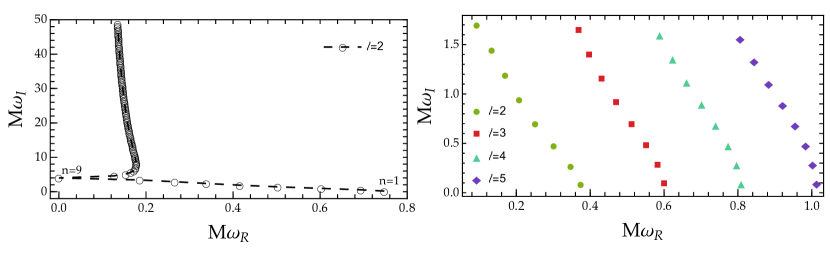
Figure 19: (Left panel) Real and imaginary part of the QNM for the first 100 overtones of the $\ell=2$ gravitational perturbations. (Right panel) Same as the left panel but for $\ell=(2,3,4,5)$ and considering the first 8 overtones. Data from tabulated values in [14].

Due to the complex nature of the frequencies, the modes diverge at both ends of the domain:

$$\textnormal{at horizon}\quad\sim e^{-i\omega r^{*}} =e^{-i\omega_{\textnormal{R}}r^{*}}e^{-\omega_{\textnormal{I}}r^{*}}\quad\xrightarrow[]{r^{*}\rightarrow-\infty}\ \infty$$ (108)

$$\textnormal{at infinity}\quad\sim e^{+i\omega r^{*}} =e^{+i\omega_{\textnormal{R}}r^{*}}e^{+\omega_{\textnormal{I}}r^{*}}\quad\xrightarrow[]{r^{*}\rightarrow+\infty}\ \infty\ .$$ (109)

Hence, QNMs carry infinite energy and do not represent a physical state across the entire space. Instead, they are a localized phenomenon that, for a fixed $r^{*}$, evolves on a given time $t$. The larger the value of $r^{*}$, the larger $t$ must be to compensate for it. Consequently, the corresponding eigenfunctions generally do not form a complete system.

5.5 Solving the master equation

There are various semi-analytical and numerical techniques that can be utilized to solve the master equation (99), provided appropriate boundary conditions, in order to search for the QNM frequencies (see [25] for a detailed review).

Direct integration.

One of the most common and efficient approaches is the direct integration method, which has a broader applicability beyond our specific case. This fully numerical framework is accurate for any value of $\ell$ (and overtones) and can be extended to different physical setups, including theories of gravity beyond General Relativity and systems involving multiple coupled fields.

As discussed in the previous section, the master equation (99) yields two solutions $\psi_{1,2}$, where $\psi_{1}$ and $\psi_{2}$ satisfy ingoing and outgoing boundary condition at the horizon and at infinity, respectively. The overall procedure can be summarized with the following steps:

1. Numerical Integration (Forward): Numerically integrate the master equation (99) forward from the horizon $r_{h}$ to infinity $r_{\infty}$, assuming as the initial condition a purely ingoing solution at $r_{h}$, namely $\psi_{1}\sim e^{-i\omega r^{*}}$. In general, to improve the accuracy of our calculations, it is useful to compute corrections to the purely ingoing solution by expanding $\psi_{1}$ around $r_{h}$ as

   $$\psi_{1}=\sum_{n=0}^{n_{h}}a_{n}(r-r_{h})^{n}e^{-i\omega r^{*}}\ ,$$ (110)

   where the order $n_{h}$ depends on the desired level of accuracy. The coefficients $a_{n}$ can be found by replacing Eq. (110) into Eq. (99) and performing a Taylor expansion around $r_{h}$. This procedure provides, order by order in $r-r_{h}$, a set of equations that can be solved for the coefficients $a_{n}$. Generally, the series of coefficients depends on the leading amplitude $a_{0}$, which can be rescaled to $a_{0}=1$ for our master equation.

2. Numerical Integration (Backward): integrate the master equation (99) backward, from infinity to the horizon. In this case, we start the integration with an initial condition that is purely outgoing at $r_{\infty}$, i.e., $\psi_{2}\sim e^{i\omega r^{*}}$. Similarly to the forward integration, we can boost the accuracy of our procedure by finding the sub-leading corrections to $\psi_{2}$ and choosing

   $$\psi_{2}=\sum_{n=0}^{n_{\infty}}\frac{b_{n}}{r^{n}}e^{i\omega r^{*}}\ .$$ (111)

   The coefficients $b_{n}$ can be found with the same procedure used for Eq. (110), but expanding the master equation around $r_{\infty}$. Even in this case, in general, $b_{n}$ will depend only on the leading term $b_{0}$, which we fix to $b_{0}=1$.

3. Given the two solutions above, we can build the Wronskian

   $$W(\omega)=\psi^{\prime}_{1}\psi_{2}-\psi^{\prime}_{2}\psi_{1}\ ,$$ (112)

   where primes denote derivatives with respect to the tortoise coordinate.

4. The QNMs of the systems are those for which the two solutions $\psi_{1,2}$ are no longer independent, corresponding to roots of the Wronskian. The overall approach translates into a findroot procedure to solve the equation $W(\omega)=0$.

WKB.

As a second technique to compute QNM frequencies, we consider the WKB approach, a semi-analytic method that builds around the analogy between the master equation (104) and the Schrodinger equation for a particle of mass $m$ and energy $E$, and a one-dimensional barrier $V(r^{*})$. Here, we follow and discuss the calculations developed in the seminal work by Schulz and Will [26]. We first consider a problem specified by the following differential equation:

$$\frac{d^{2}\psi(r^{*})}{(dr^{*})^{2}}+Q(r^{*})\psi(r^{*})=0\ ,$$ (113)

which resembles our master equation with $Q=\omega^{2}-V_{s}$. As seen for the scalar case, the function $\psi(r^{*})$ identifies the radial component of the full solution, which depends on time $(\sim e^{-i\omega t})$ and on the angular variables.

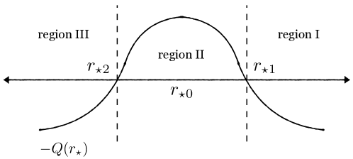
Figure 20: Representation of the function $-Q(x)$. Adapted from [26].

The function $-Q(r^{*})$ depends on the tortoise coordinate, has a maximum around $r^{*}\simeq 0$, and approaches a constant $Q(r^{*})\rightarrow\alpha$ with $\real(\alpha)>0$ at both ends of the domain, such that the solution reads

$$\frac{d^{2}\psi(r^{*})}{(dr^{*})^{2}}+\alpha\psi(r^{*})=0\ ,\qquad\Rightarrow\qquad\psi(r^{*})\sim e^{\pm i\alpha r^{*}}\ ,\qquad|r^{*}|\rightarrow\infty\ ,$$ (114)

with $e^{-i\alpha r^{*}}$ ($e^{i\alpha r^{*}}$) being outgoing (ingoing) modes at $+\infty$ ($-\infty$). The basic idea behind the WKB approach is to study the behaviour of $Q(r^{*})$ in the three zones in which the function is defined, finding the matching conditions across them. Figure 20 provides a pictorial representation of the regions I, II, III, and the turning points $r_{1}^{*},r_{2}^{*}$, where $Q(r_{1}^{*})=Q(r_{2}^{*})=0$. In the first and third regions, the solutions for the master equation can be found analytically [27]:

$$Q(r^{*})=\begin{cases}Q^{-1/4}(r^{*})\exp\left[\pm i\int^{r^{*}}_{r_{1}^{*}}\!dx\,\sqrt{Q(x)}\right]\ ,&\textnormal{region I}\ ,\\ \\ Q^{-1/4}(r^{*})\exp\left[\pm i\int^{r_{2}^{*}}_{r^{*}}\!dx\,\sqrt{Q(x)}\right]\ ,&\textnormal{region III}\ .\end{cases}$$ (115)

We want now to match these solutions with region II, which is bounded by the turning points where $Q(r^{*})=0\rightarrow V_{s}(r^{*})=\omega^{2}$. The WKB approach works better when $r_{1}^{*}$ and $r_{2}^{*}$ are close, i.e., when $|Q(\pm\infty)|\gg[-Q(r^{*})]_{\textnormal{peak}}$ and $V_{\textnormal{peak}}\sim\omega^{2}$. Following [26], we approximate $Q(r^{*})$ in this central zone with a parabola:

$$Q(r^{*})=Q_{0}+\frac{1}{2}Q^{\prime\prime}_{0}(r^{*}-r_{0}^{*})^{2}+\mathcal{O}(r^{*}-r_{0}^{*})^{3}\ ,$$ (116)

with $Q_{0}<0$ and $Q^{\prime\prime}_{0}>0$. We now introduce the new variable $t=(4\kappa)^{1/4}e^{i\pi/4}(r^{*}-r_{0}^{*})$, where $\kappa=Q_{0}^{\prime\prime}/2$, such that Eq. (113) can be recast in the following form:

$$\begin{gathered}\frac{d^{2}\psi(t)}{dt^{2}}(4\kappa)^{1/2}e^{i\pi/2}+\left[Q_{0}+\frac{1}{2}\frac{2\kappa t^{2}}{(4\kappa)^{1/2}e^{i\pi/2}}\right]\psi(t)=0\ ,\\ \Rightarrow\quad\frac{d^{2}\psi(t)}{dt^{2}}+\left[-\frac{iQ_{0}}{(2Q_{0}^{\prime\prime})^{1/2}}-\frac{t^{2}}{4}\right]\psi(t)=0\ .\end{gathered}$$ (117)

We further introduce the parameter $\nu=-\frac{1}{2}-\frac{iQ_{0}}{(2Q_{0}^{\prime\prime})^{1/2}}$, such that

$$\frac{d^{2}\psi}{dt^{2}}+\left[\nu+\frac{1}{2}-\frac{t^{2}}{4}\right]\psi(t)=0\ ,$$ (118)

whose solution is given as a combination of parabolic cylinder functions, $D_{\nu}(t)$:

$$\psi(t)=AD_{\nu}(t)+BD_{-1-\nu}(it)\ .$$ (119)

Exploiting the asymptotic properties of these functions, near the horizon we find:

$$\psi \sim c_{1}(1-i)^{\nu}e^{i\pi\nu/2}\kappa^{\nu/4}(r^{*}-r_{0}^{*})^{\nu}e^{-i\kappa^{1/2}(r^{*}-r_{0}^{*})^{2}/2}$$ (120)

$$\qquad+e^{-\frac{3}{4}i\pi\nu}2^{-\nu/2}\kappa^{-(1+\nu)/4}(r^{*}-r_{0}^{*})^{-1-\nu}\left[c_{2}-c_{1}\frac{ie^{-i\pi\nu/2}\sqrt{2\pi}}{\Gamma(-\nu)}\right]e^{i\kappa^{1/2}(r^{*}-r_{0}^{*})^{2}/2}\ ,$$

with $c_{1,2}$ as constants of integration, and $\Gamma(\nu)$ being the Euler Gamma function. The first and second terms of this expression identify ingoing and outgoing waves. Boundary conditions require that at the horizon, the outgoing modes are zero, which fixes $c_{2}=0$ and $\Gamma(-\nu)=\infty$. The latter holds if $\nu$ is an integer. This requirement automatically translates into a Born–Sommerfield quantization rule, such that

$$\frac{Q_{0}}{\sqrt{2Q_{0}^{\prime\prime}}}=i\left(n+\frac{1}{2}\right)\ ,\qquad n=0,1,2,\dots\ .$$ (121)

The function $Q$ depends on the frequency $\omega$, hence Eq. (121) turns into an algebraic relation which identifies a discrete set of complex values, the quasi-normal mode frequencies. For gravitational perturbations of a Schwarzschild BH, $Q$ is given by Eq. (104) (with $s=2$), with the peak provided by Eq. (103), allowing the computation of the values of $\omega$ for different $\ell$ and $n$. The WKB approximation works well for low overtones, i.e., as we have seen in Fig. 19 for modes with small imaginary parts (or large damping times), and for large $\ell$. The relative difference between the Schwarzschild QNM frequencies obtained with the WKB and the exact values of [14] is shown in Fig. 21 for $\ell=(2,3,4,5)$ and the first three overtones. The accuracy of the WKB method can be improved considering different approximations of the function $-Q(x)$ though region II and taking into account, for example, higher-order approximations which go beyond the quadratic expansion [28, 29].

Figure 21: (Left panel) Relative difference between the real and imaginary part of the QNM computed with the WKB approach and the values obtained in [14], as a function of $\ell$ for the first three overtones.

6 Conclusions

In this notes, we have explored the key features of non-rotating black holes in General Relativity. Alongside the properties of the Schwarzschild solution, we examined in detail the motion of massive and massless test-bodies, along with their fundamental frequencies.

We introduced a general framework for computing relativistic perturbations of spherically-symmetric and static spacetimes. Instead of elaborating on all the calculations required for tensor perturbations, we focused on the response induced by a test scalar field propagating on a fixed geometry. This approach allowed us to control perturbations using a single master equation, which can be extended to more complicated scenarios involving vector and tensor modes. Consequently, we introduced the concept of black hole oscillations. We have discussed the main properties of the Schwarzschild quasi-normal modes and their connection with the dynamics of massless particles in the background spacetime. Finally, we described two numerical methods, namely, the direct integration and the WKB approach, commonly used to compute the actual values of quasi-normal modes.

References

- [1] LIGO Scientific, VIRGO, KAGRA Collaboration, R. Abbott et al., “GWTC-3: Compact Binary Coalescences Observed by LIGO and Virgo During the Second Part of the Third Observing Run,” arXiv:2111.03606 [gr-qc].
- [2] M. Branchesi et al., “Science with the Einstein Telescope: a comparison of different designs,” JCAP 07 (2023) 068, arXiv:2303.15923 [gr-qc].
- [3] M. Evans et al., “Cosmic Explorer: A Submission to the NSF MPSAC ngGW Subcommittee,” arXiv:2306.13745 [astro-ph.IM].
- [4] LISA Collaboration, P. A. Seoane et al., “Astrophysics with the Laser Interferometer Space Antenna,” Living Rev. Rel. 26 no. 1, (2023) 2, arXiv:2203.06016 [gr-qc].
- [5] E. Berti et al., “Testing General Relativity with Present and Future Astrophysical Observations,” Class. Quant. Grav. 32 (2015) 243001, arXiv:1501.07274 [gr-qc].
- [6] L. Barack et al., “Black holes, gravitational waves and fundamental physics: a roadmap,” Class. Quant. Grav. 36 no. 14, (2019) 143001, arXiv:1806.05195 [gr-qc].
- [7] E. Berti, K. Yagi, H. Yang, and N. Yunes, “Extreme Gravity Tests with Gravitational Waves from Compact Binary Coalescences: (II) Ringdown,” Gen. Rel. Grav. 50 no. 5, (2018) 49, arXiv:1801.03587 [gr-qc].
- [8] E. Berti, K. Yagi, and N. Yunes, “Extreme Gravity Tests with Gravitational Waves from Compact Binary Coalescences: (I) Inspiral-Merger,” Gen. Rel. Grav. 50 no. 4, (2018) 46, arXiv:1801.03208 [gr-qc].
- [9] K. D. Kokkotas and B. G. Schmidt, “Quasinormal modes of stars and black holes,” Living Rev. Rel. 2 (1999) 2, arXiv:gr-qc/9909058.
- [10] V. Ferrari and L. Gualtieri, “Quasi-Normal Modes and Gravitational Wave Astronomy,” Gen. Rel. Grav. 40 (2008) 945–970, arXiv:0709.0657 [gr-qc].
- [11] E. Berti, V. Cardoso, and A. O. Starinets, “Quasinormal modes of black holes and black branes,” Class. Quant. Grav. 26 (2009) 163001, arXiv:0905.2975 [gr-qc].
- [12] S. L. Detweiler, “Black holes and gravitational waves. iii - The resonant frequencies of rotating holes,” Astrophys. J. 239 (1980) 292–295.
- [13] O. Dreyer, B. J. Kelly, B. Krishnan, L. S. Finn, D. Garrison, and R. Lopez-Aleman, “Black hole spectroscopy: Testing general relativity through gravitational wave observations,” Class. Quant. Grav. 21 (2004) 787–804, arXiv:gr-qc/0309007.
- [14] E. Berti, V. Cardoso, and C. M. Will, “On gravitational-wave spectroscopy of massive black holes with the space interferometer LISA,” Phys. Rev. D 73 (2006) 064030, arXiv:gr-qc/0512160.
- [15] N. Franchini and S. H. Völkel, “Testing General Relativity with Black Hole Quasi-Normal Modes,” arXiv:2305.01696 [gr-qc].
- [16] V. Cardoso and P. Pani, “Testing the nature of dark compact objects: a status report,” Living Rev. Rel. 22 no. 1, (2019) 4, arXiv:1904.05363 [gr-qc].
- [17] M. Nakahara, Geometry, Topology and Physics. CRC Press, 2018.
- [18] S. Weinberg, Gravitation and Cosmology: Principles and Applications of the General Theory of Relativity. Wiley, 1972.
- [19] S. Carroll, Spacetime and Geometry. Cambridge University Press, 2019.
- [20] H. Abolghasem, “Stability of circular orbits in Schwarzschild space-time,” J. Dyn. Syst. Geom. Theor. 10 (2012) 13–32.
- [21] W. Boyce and R. DiPrima, Elementary differential equations and boundary value problems. Wiley New York, 8th ed., 2004.
- [22] C. L. Lewis, “Explicit gauge covariant Euler–Lagrange equation,” Am. J. Phys. 77 no. 9, (Sep, 2009) 839–843. https://doi.org/10.1119%2F1.3153503.
- [23] E. Berti, “A Black-Hole Primer: Particles, Waves, Critical Phenomena and Superradiant Instabilities,” 10, 2014. arXiv:1410.4481 [gr-qc].
- [24] S. Chandrasekhar, “On Algebraically Special Perturbations of Black Holes,” Proceedings of the Royal Society of London. Series A, Mathematical and Physical Sciences 392 no. 1802, (1984) 1–13. http://www.jstor.org/stable/2397739.
- [25] P. Pani, “Advanced Methods in Black-Hole Perturbation Theory,” Int. J. Mod. Phys. A 28 (2013) 1340018, arXiv:1305.6759 [gr-qc].
- [26] B. F. Schutz and C. M. Will, “Black hole normal modes - A semianalytic approach,” ApJL 291 (Apr., 1985) L33–L36.
- [27] C. M. Bender and S. A. Orszag, Advanced Mathematical Methods for Scientists and Engineers. McGraw-Hill, 1978.
- [28] S. Iyer, “Black-hole normal modes: A WKB approach. II. Schwarzschild black holes,” Phys. Rev. D 35 (Jun, 1987) 3632–3636. https://link.aps.org/doi/10.1103/PhysRevD.35.3632.
- [29] R. A. Konoplya, “Quasinormal behavior of the -dimensional Schwarzschild black hole and the higher order WKB approach,” Phys. Rev. D 68 (Jul, 2003) 024018. https://link.aps.org/doi/10.1103/PhysRevD.68.024018.