From a distance: Shuttleworth revisited

Abstract

The Shuttleworth equation: a linear stress-strain relation ubiquitously used in modeling the behavior of soft surfaces. Its validity in the realm of materials subject to large deformation is a topic of current debate. Here, we zoom out to derive the constitutive behavior of the surface from the general framework of finite kinematics. We distinguish cases of finite and infinitesimal surface relaxation prior to an infinitesimal applied deformation. The Shuttleworth equation identifies as the Cauchy stress measure in the fully linearized setting. We show that in both finite and linearized cases, measured elastic constants depend on the utilized stress measure. In addition, we discuss the physical implications of our results and analyze the magnitude of surface relaxation in the light of two different test cases.

Introduction

In most solids, small forces lead to small deformations. A soft solid, on the contrary, can experience large deformations under minute forces: a phenomenon as minor as depositing a millimetric droplet leads to divergent deformations of its surface Style et al. (2017); Andreotti and Snoeijer (2020); Style et al. (2013a); Hui and Jagota (2014) (Fig. 1). Such materials, which can take the form of gels, pastes, or elastomers, are ubiquitous in our lives: They amount to most of our body tissues, and can be used as lubricants, glues, and water-repellent coatings. In past years, it has been shown that surface stresses are essential in wetting, adhesion, and fracture, and can be harvested in composites  Style et al. (2017); Andreotti and Snoeijer (2020); Style et al. (2013a); Hui and Jagota (2014); Smith-Mannschott et al. (2021); Schulman et al. (2018); Hui et al. (2020); Style et al. (2013b); Jensen et al. (2015); Grzelka et al. (2017); Style et al. (2015). Yet, the physical origins of surface stresses are poorly understood. This statement is especially true in gels, in which cohabitation of a crosslinked polymer network and a liquid solvent complexifies the link between molecular structure and mechanical properties.

To tackle this fundamental question, the dominant approach is to investigate surface elastic properties Bain et al. (2021); Heyden et al. (2021, 2022); Carbonaro et al. (2020); Xu et al. (2018). For instance, surface topography measurements of a stretched patterned silicone gel revealed an elastic surface, with surface stresses that increase with surface deformations Bain et al. (2021). This result hints towards a role of the crosslinked polymeric network in the surface constitutive behavior of silicone gels. On the contrary, deformation measures of a spinning hydrogel bead evidenced a constant surface stress, independent of surface deformations, akin to the surface tension of the solvent Carbonaro et al. (2020).

In its simplest form, the most common description for the surface mechanics of soft solids relates the surface stresses $\bm{\Upsilon}_{s}$ to the surface strains $\bm{\epsilon}_{s}$ and free energy $W_{s}$,

$$\bm{\Upsilon}_{s}=W_{s}\bm{I}+\frac{\partial W_{s}}{\partial\bm{\epsilon}_{s}},$$ (1)

and is commonly called the Shuttleworth equation Shuttleworth (1950). This description is restricted to the linear regime, in which small deformations prevail. It is, however, largely applied to surfaces that undergo large deformations. In this setting, its validity and the physical interpretations that follow have been rightfully questioned Gutman (2022); Bain et al. (2022); Pandey et al. (2020); Masurel et al. (2019). In parallel, extensive works in continuum mechanics laid out the framework of surface elasticity (see, e.g., Gurtin and Murdoch (1975); Gurtin et al. (1998); Huang and Wang (2007); Krichen et al. (2019); Mozaffari et al. (2020)). Here, we aim to link both paths.

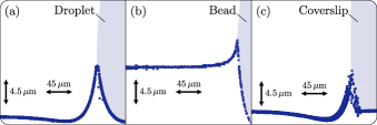
Figure 1: Experimental surface profiles of a initially flat soft solids in contact with (a) a drop of glycerol, (b) a silica bead and (c) a glass coverslip. The data were obtained from confocal imaging of fluorescent beads deposited on a silicone gel of shear modulus $\mu\sim 2\,\mbox{kPa}$ (same protocol as Jagota et al. (2012); Style et al. (2013a); Xu et al. (2017, 2018)). Each blue circle represents a detected fluorescent bead, and the light blue areas schematically represent the contacting objects.

The major drawback of the Shuttleworth equation is that it neglects the bigger picture. Hence, any features stemming from a differentiation between initial and final configurations are lost. In the following, we take advantage of the framework of finite kinematics to rigorously derive the surface stress-strain relation from a strain energy density. Prior to an applied deformation, soft solids are usually detached from a container and their surfaces undergo an initial relaxation, which induces residual bulk stresses. Because soft solids are easy to deform, this surface relaxation can be large Jagota et al. (2012); Mora et al. (2013). We distinguish cases of infinitesimal and finite surface relaxation. We highlight cases in which different stress measures do not coincide upon linearization. The given framework should incite experimentalists to choose the most suitable stress-strain relation and carefully interpret measured surface elastic parameters. We exemplify this interpretation considering two different test cases.

Finite kinematics

General case

We start with a brief outline of the basic finite kinematics setting. Let us consider a solid in two states. A reference state, prior to being deformed, and a deformed state (Fig. 2). In the reference state, it is well established that the surface exhibits mechanical stresses, which in the simplest case have the form of a uniform and isotropic surface tension Style et al. (2017); Andreotti and Snoeijer (2020). Let us furthermore assume that the surface stresses can be thermodynamically defined by a surface strain energy density $W^{\rm R}$ in the reference configuration.

Following the Piola transform specialized to two dimensions, we can define a free energy density expressed in the current configuration $W^{\rm C}$ as

$$\int_{S}W^{\rm C}\,dS=\int_{S_{\rm R}}W^{\rm C}J_{s}\,dS_{\rm R}=\int_{S_{R}}\,W^{\rm R}\,dS_{R},$$ (2)

with $S_{R}$ and $S$ the areas in the reference- and current configurations, respectively. Furthermore, $J_{s}=\text{det}(\bm{F}_{s})=\text{det}(\bm{I}+\bm{\nabla}_{s}\bm{u})$ measures the local change in area, where $\bm{F}_{s}$ is the deformation gradient and $\bm{u}$ the displacement field (details are given in Supplementary Section 1). Based on material frame indifference, any strain energy density can be written as a function of the Green-Lagrange strain tensor $\bm{E}_{s}=\frac{1}{2}(\bm{F}_{s}^{\rm T}\bm{F}_{s}-\bm{I})$. Here, as in the rest of the manuscript, all vector quantities, such as displacement fields, and all tensor quantities, such as stress- and strain fields, are projected onto the surface (see Supplementary Section 1 for details).

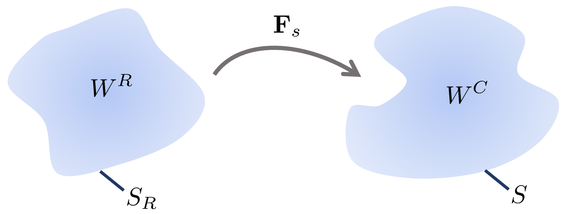
Figure 2: Sketch of reference configuration (left) and deformed configuration (right).

Depending on the experimental conditions, different stress measures may be used for comparison to theory. The first Piola-Kirchhoff stress measure $\bm{P}_{s}$, also known as the engineering stress, represents forces in the current configuration per unit referential area. Therefore, it is likely the quantity of interest in traction-controlled experiments Mozaffari et al. (2020). In contrast, the second Piola-Kirchhoff stress measure $\bm{S}_{s}$ constitutes forces mapped back to the reference configuration per unit referential area. Finally, the Cauchy stress measure $\bm{\sigma}_{s}$, also denoted as true stress, refers to forces in the current configuration per unit current area. It is then the stress measure used in a Eulerian setting, or phenomena where the reference state is ill defined, as in liquid flows. By definition, the second Piola-Kirchhoff stress derives directly from the free energy density in the reference configuration,

$$\bm{S}_{s}=\frac{\partial W^{\rm R}}{\partial\bm{E}_{s}},$$ (3)

and the two other stress measures account for the change of reference frame by multiplication with the deformation gradient

$$\bm{P}_{s}=\bm{F}_{s}\frac{\partial W^{\rm R}}{\partial\bm{E}_{s}}\text{, and }\bm{\sigma}_{s}=J_{s}^{-1}\bm{F}_{s}\frac{\partial W^{\rm R}}{\partial\bm{E}_{s}}\bm{F}_{s}^{\rm T}.$$ (4)

If one considers the free energy in the current configuration Eq.(2), as is implicitly assumed in the Shuttleworth equation, the Cauchy stress takes a form similar to Eq.(1)

$$\bm{\sigma}_{s}=W^{\rm C}\mathbf{I}+\bm{F}_{s}\frac{\partial W^{\rm C}}{\partial\bm{E}_{s}}\bm{F}_{s}^{\rm T},$$ (5)

and the other stresses measures also have a similar expression (see Supplementary Section 2 for details).

At this point, it is instructive to define a constitutive equation for the surface free energy. If we assume the surface energy to be strain-independent $W^{\rm C}=\gamma$, as in liquids, the Cauchy stresses Eq. (5) correspond to a liquid-like isotropic surface tension $\bm{\sigma}_{s}=\gamma\mathbf{I}$.

For a strain-dependent surface energy, without loss of generality we use the St. Venant-Kirchhoff model, which is the simplest extension of linear elasticity that accounts for geometric nonlinearities. To account for the surface tension in the reference state, we enrich this model with a constant surface energy in the current configuration,

$$W^{R}(\bm{E}_{s})=\gamma\,J_{s}+\mu_{s}\,\text{tr}(\bm{E}_{s}\bm{E}_{s})+\frac{1}{2}\lambda_{s}(\text{tr}(\bm{E}_{s}))^{2}.$$ (6)

Here, $\mu_{s}$ and $\lambda_{s}$ are the surface shear modulus and surface Lamé parameter, respectively. Physically speaking, $\gamma$ is equivalent to the surface tension of a liquid, while $(\mu_{\rm s},\lambda_{\rm s})$ are the surface elastic constants attributing an energetic cost to elastic deformation from a reference state. In this framework, a simple derivation leads to the Cauchy stress as a function of the elastic parameters

$$\bm{\sigma}_{s}=\gamma\bm{I}+\bm{F}_{s}\left(2\mu_{s}\bm{E}_{s}+\lambda_{s}\text{tr}(\bm{E}_{s})\bm{I}\right)\bm{F}_{s}^{T},$$ (7)

and similarly to the first and second Piola-Kirchhoff stresses

$$\bm{P}_{s} =\gamma J_{s}\bm{F}_{s}\left(\bm{F}_{s}^{\rm T}\bm{F}_{s}\right)^{-1}+2\mu_{s}\bm{F}_{s}\bm{E}_{s}+\lambda_{s}\text{tr}(\bm{E}_{s})\bm{F}_{s},$$ (8)

$$\bm{S}_{s} =\gamma J_{s}\left(\bm{F}_{s}^{\rm T}\bm{F}_{s}\right)^{-1}+2\mu_{s}\bm{E}_{s}+\lambda_{s}\text{tr}(\bm{E}_{s})\bm{I}.$$ (9)

The case of soft solids

Soft solids are often cured within a mold, from which they are detached before being used. Upon detachment, soft solids undergo a surface relaxation due to the change of interface, and enhanced wherever the local curvature is nonzero Jagota et al. (2012); Mora et al. (2013); Hui et al. (2020). We therefore distinguish three mechanical states (Fig. 3). The soft solid with the shape of the mold before it relaxes, $\Omega^{*}$, after relaxed from the mold but prior to any external load or displacement, $\Omega_{0}$, and after being deformed by external loads $\Omega$.

In the first, fictitious state $\Omega^{*}$, the bulk of the soft solid is stress-free. For this reason, we will use this state as the reference configuration (Fig. 2). The surface, however, is not stress-free, as is accounted for in our definition of the surface energy Eq. (6). While the second state, $\Omega_{0}$, is the one experimentalists physically work with, we will consider it as an intermediate state because it contains potentially finite residual bulk stresses due to prior surface relaxation. We note, however, that these two states coincide when the surface does not undergo prior relaxation, which happens when the soft solid is tested in the state it was prepared.

In the framework of finite kinematics, the deformation gradient $\bm{F}_{s}$ maps material points from the stress-free configuration $\Omega^{*}$ to the deformed configuration $\Omega$. We also have $\bm{F}^{*}_{s}=\bm{I}+\bm{\nabla}_{s}\bm{u}^{*}$ mapping from the stress-free configuration $\Omega^{*}$ to the relaxed configuration $\Omega_{0}$, and $\bm{F}^{0}_{s}=\bm{I}+\bm{\nabla}_{s}\bm{u}^{0}$ mapping from the relaxed configuration $\Omega_{0}$ to the deformed configuration $\Omega$. By composition of mappings, the total deformation follows as $\bm{F}_{s}=\bm{F}^{0}_{s}\bm{F}^{*}_{s}$.

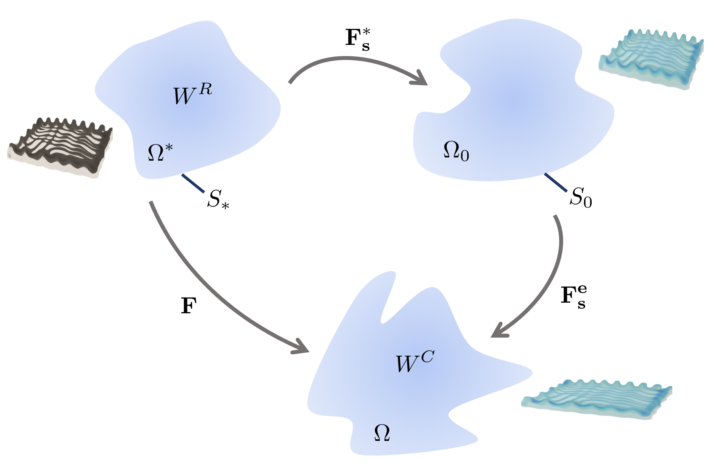
Figure 3: Sketch of fictitious stress-free configuration $\Omega^{*}$, e.g., a cured sample within a mold), relaxed configuration $\Omega_{0}$, e.g., a sample after removal from the mold, and deformed configuration $\Omega$. The stress-free and the current configurations have a surface strain energy density $W^{\rm R}$ and $W^{\rm C}$, respectively.

Linearized Kinematics

In practice, experiments most easily impose deformations $\bm{E}^{0}_{s}$, from the relaxed state $\Omega_{0}$ to the deformed state $\Omega$. Here, we will focus on the case where the imposed deformations are small, for which $\bm{E}^{0}_{s}\sim\bm{\epsilon}^{0}_{s}$. We then elucidate how the measured stresses vary with imposed surface strain $\bm{\epsilon}^{0}_{s}=[\bm{\nabla}_{s}\bm{u}^{0}+(\bm{\nabla}_{s}\bm{u}^{0})^{T}]/2$, both when the relaxation deformation $\bm{E}^{*}_{s}$ is infinitesimal and finite.

Infinitesimal surface relaxation

Let us assume that the deformation due to the relaxation of the surface is small $\bm{E}^{*}_{s}\sim\bm{\epsilon}^{*}_{s}$. In this scenario, the resultant total strain is a simple additive decomposition $\bm{\epsilon}_{s}=\bm{\epsilon}_{s}^{*}+\bm{\epsilon}_{s}^{0}$.

After linearization, stress measures are usually assumed to coincide. This assumption, however, is not true when initial stresses are present Krichen et al. (2019), as in the case of solid surfaces. We thus need to carefully distinguish different stress measures in the realm of linearized kinematics. At first order in strains $\bm{\epsilon}_{s}=(\bm{\nabla}_{s}\bm{u}+\bm{\nabla}_{s}\bm{u}^{T})/2$, the linearized Cauchy stress $\tilde{\bm{\sigma}}$ simplifies to the Hookean form

$$\tilde{\bm{\sigma}}_{s}=\gamma\bm{I}+2\mu_{s}\bm{\epsilon}_{s}+\lambda_{s}\text{tr}(\bm{\epsilon}_{s})\bm{I}.$$ (10)

Based on the additive decomposition of strains, Cauchy stresses result in a contribution from the surface relaxation $\tilde{\bm{\sigma}}_{s}^{*}$ and a contribution from the imposed deformations $\tilde{\bm{\sigma}}_{s}^{0}$

$$\tilde{\bm{\sigma}}_{s}=\gamma\bm{I}+\tilde{\bm{\sigma}}_{s}^{*}+\tilde{\bm{\sigma}}_{s}^{0},$$ (11)

where $\tilde{\bm{\sigma}}_{s}^{\alpha}=2\mu_{s}\bm{\epsilon}_{s}^{\alpha}+\lambda_{s}\text{tr}(\bm{\epsilon}_{s}^{\alpha})\bm{I}$. Unsurprisingly, the surface relaxation here only comes as an additive stress. It will therefore not influence the estimation of the surface elastic moduli $\mu_{s}$ and $\lambda_{s}$.

Similarly, the second Piola-Kirchhoff stress takes the form

$$\tilde{\bm{S}}_{s}=\gamma\bm{I}+2\mu_{s}^{S}\bm{\epsilon}_{s}+\lambda_{s}^{S}\text{tr}(\bm{\epsilon}_{s})\bm{I},$$ (12)

with effective elastic constants $\mu_{s}^{S}=\mu_{s}-\gamma$ and $\lambda_{s}^{S}=\lambda_{s}+\gamma$. The first Piola-Kirchhoff stress is non-symmetric

$$\tilde{\bm{P}}_{s}=\gamma\bm{I}+2\mu_{s}^{P}\bm{\epsilon}_{s}+\lambda_{s}^{P}\text{tr}(\bm{\epsilon}_{s})\bm{I}+\gamma^{C}\bm{\omega}_{s},$$ (13)

with $\mu_{s}^{P}=\mu_{s}-\gamma/2$, $\lambda_{s}^{P}=\lambda_{s}^{S}$, and $\bm{\omega}_{s}=(\bm{\nabla}_{s}\bm{u}-\bm{\nabla}_{s}\bm{u}^{T})/2$ the infinitesimal rotation tensor (see Supplementary Section 3 for details of the linearization). Both the first and second Piola-Kirchhoff stress measures can also be decomposed akin to the Cauchy stress Eq. (11).

From Eqs. (10) to (13), we note that the three linearized stress measures are only equal in two scenarios. First, when the solid is unstretched $\bm{\epsilon}_{s}=0$. All stress measures are then trivially equal to the prestress $\gamma\mathbf{I}$, which is the surface tension of the solid at rest. Second, when the prestress is much smaller than the surface elastic constants $\gamma\ll(\mu_{\rm s},\lambda_{\rm s})$. In this case, which primarily pertains to hard solids, all stress measures are equal to the Hookean form Eq.(10). Besides these cases, however, linearized stress measures need to be carefully distinguished from each other. This applies not only to soft solids, for which surface tension and surface elasticity can be of the same order of magnitude Bain et al. (2021); Heyden et al. (2022), but also for complex fluid-fluid interfaces Fuller and Vermant (2012).

Finite surface relaxation

If the surface relaxation induces large deformations, we expand to linear order in $\bm{\nabla}\bm{u}^{0}$ the imposed deformations and keep the relaxation deformations $\bm{F}^{*}$ finite. At first order, we write the dependence of Cauchy stress with imposed deformations

$$\bar{\bm{\sigma}}_{s}= \,\gamma\bm{I}+\bar{\bm{\sigma}}^{*}_{s}+\bm{\nabla}\bm{u}^{0}\bar{\bm{\sigma}}^{*}_{s}+\bar{\bm{\sigma}}^{*}_{s}(\bm{\nabla}\bm{u}^{0})^{T}$$

$$+2\mu_{s}[\bm{F}_{s}^{*}(\bm{F}_{s}^{*})^{T}]\bm{\epsilon}^{0}_{s}[\bm{F}_{s}^{*}(\bm{F}_{s}^{*})^{T}]$$

$$+\lambda_{s}\text{tr}[(\bm{F}_{s}^{*})^{T}\bm{\epsilon}^{0}_{s}\bm{F}_{s}^{*}]\bm{F}_{s}^{*}(\bm{F}_{s}^{*})^{T},$$ (14)

where $\bar{\bm{\sigma}}^{*}_{s}=\bm{F}^{*}_{s}\left(2\mu_{s}\bm{E}^{*}_{s}+\lambda_{s}\text{tr}(\bm{E}^{*}_{s})\bm{I}\right)(\bm{F}^{*}_{s})^{T}$ is the stress contribution due to surface relaxation (see Supplementary Section 3 for details, and Supplementary Section 4 for a full derivation in the absence of surface shear). Here, not only does the relaxation impose an additional stress term $\bar{\bm{\sigma}}^{*}_{s}$, it also mixes non-trivially into the terms that include the surface elastic parameters $(\lambda_{s},\mu_{s})$. In practice, the exact contribution from the finite surface relaxation depend on the sample geometry and has to be estimated accordingly. For the sake of completeness, we estimate the strain dependence of the Second Piola-Kirchhoff stress as

$$\bar{\bm{S}}_{s} =\bar{\bm{S}}_{s}^{*}+\gamma J_{s}^{*}(\bm{F}_{s}^{*})^{-1}\left[\text{tr}(\bm{\epsilon}^{0})-2\bm{\epsilon}^{0}_{s}\right](\bm{F}_{s}^{*})^{-T}$$

$$+2\mu_{s}(\bm{F}_{s}^{*})^{T}\bm{\epsilon}^{0}_{s}\bm{F}_{s}^{*}+\lambda_{s}\text{tr}((\bm{F}_{s}^{*})^{T}\bm{\epsilon}^{0}_{s}\bm{F}_{s}^{*})\bm{I}.$$ (15)

Finally, the First Piola-Kirchhoff stress tensor follows as

$$\bar{\bm{P}}_{s}=\bm{F}_{s}^{*}\bar{\bm{S}}_{s}+\bm{\nabla}_{s}\bm{u}^{0}\bar{\bm{S}}_{s}^{*},$$ (16)

where $\bar{\bm{S}}_{s}^{*}=\gamma J_{s}^{*}\left[(\bm{F}_{s}^{*})^{\rm T}\bm{F}_{s}^{*}\right]^{-1}+2\mu_{s}\bm{E}_{s}^{*}+\lambda_{s}\text{tr}(\bm{E}_{s}^{*})\bm{I}$ is the Second Piola-Kirchhoff stress contributions to surface relaxation. Although the expressions (14) to (16) are cumbersome, we note that they do not coincide even in the case of no imposed deformations $\bm{\epsilon}_{s}^{0}=\bm{0}$.

Overall, whether the surface relaxation induces small or finite deformations, the different stress measures differ from each other. While we can extract effective surface elastic coefficients in the case of infinitesimal surface relaxation (Eqs. (10) to (13)), accounting for finite relaxation (Eqs. (14) to (16)) prevents having a simple constitutive equation between stresses and imposed deformation $\bm{\nabla}_{s}\epsilon^{0}_{s}$.

Estimation of the surface relaxation

To understand when surface relaxation induces infinitesimal or finite surface strains, we examine how an incompressible soft solid of shear modulus $\mu$ and surface tension $\gamma$ responds in two canonical examples. As we are looking for an estimate of the surface strain we do not account for surface elasticity effects, which would be of higher order.

Figure 4: (a) Surface profile of periodic grooves of wavelength $w$. Left: initial profile, with amplitude $a_{0}$. Right: after relaxation, with amplitude $a_{1}$, estimated for a material of shear modulus $\mu=2\,\rm kPa$, surface tension $\gamma=20\,\rm mN/m$, wavelength $w=50\,\mu\rm m$ and initial amplitude $a_{0}=2\,\mu\rm m$. (b) Cylindrical rod before (left) and after relaxation (right). (c) Contour plot for the surface relaxation axial strain $\epsilon_{s\parallel}$ as a function of shear modulus and cylinder radius, computed from Eq.(19) with surface tension $\gamma=20\,\rm mN/m$. The black dashed line represents stands for $R=L_{\rm ec}$. (d) Deviation factors $P$ and $L$, quantifying the effect of surface relaxation on estimated surface modulus (Eqs.(17) and (20)).

First, we assume that it is cured into a mold with periodic rectangular grooves of wavelength $w$ and initial amplitude $a_{0}$. For simplicity, we assume that the solid is much thicker than the pattern wavelength, akin to the experimental system in Bain et al. (2021). After demolding, the surface topography relaxes to a nearly rectangular wave with final amplitude $a_{1}\sim a_{0}/(1+|q|L_{\rm ec})$, where $q=2\pi/w$ is the pattern wavevector and $L_{\rm ec}=\gamma/2\mu$ is the elastocapillary length Jagota et al. (2012); Hui et al. (2020); Bain et al. (2021) (Fig. 4a). During this process, one period of the surface goes from its initial length $l_{0}=w+2a_{0}$ to a final length $l_{1}\sim w+2a_{1}$. We define the surface relaxation strain $\epsilon_{s}^{*}=(l_{1}-l_{0})/l_{0}$ from the difference in surface length before and after demolding.

In this simplified example, we distinguish two regimes. When the pattern is very flat, $a\ll w$, the surface strain $\epsilon_{s}^{*}\sim(a_{1}-a_{0})/w$ is always infinitesimal and we can use the fully linearized framework (Eqs. (10) to (13)). When the pattern is not flat, i.e., the amplitude is either comparable to or larger than the wavelength, the surface strain $\epsilon_{s}^{*}\sim(a_{1}-a_{0})/a_{0}\sim qL_{\rm ec}/(1+qL_{\rm ec})$ is infinitesimal when the wavelength is much larger than the elastocapillary length, $qL_{\rm ec}\ll 1$, and finite when the wavelength is smaller than or comparable to $L_{\rm ec}$. In this last case, we have to account for finite relaxations (Eqs. (14) to (16)). To do so, we assume the surface relaxation strains are tangential to the surface profile $\left(\epsilon_{\rm s\parallel}^{*},\epsilon_{\rm s\perp}^{*}\right)=\left(\epsilon_{\rm s}^{*},0\right)$, and that we impose an external deformation that manifests as a longitudinal strain $\epsilon_{\rm s}^{0}$. The longitudinal Cauchy stress,

$$\bar{\sigma}_{\rm s\parallel}=\gamma+\bar{\sigma}_{\rm s\parallel}^{*}+(2\mu_{\rm s}+\lambda_{\rm s})P(\epsilon_{\rm s}^{*})\epsilon_{\rm s}^{0},$$ (17)

is then linear in imposed strain $\epsilon_{\rm s}^{0}$ and polynomial in relaxation strains $P(\epsilon)=(1+\epsilon)^{2}\left(1+4\epsilon+2\epsilon^{2}\right)$. When the surface relaxation strain is infinitesimal $\epsilon_{\rm s}^{*}\ll 1$, we recover the surface modulus $(2\mu_{\rm s}+\lambda_{\rm s})$ that can be calculated from the fully linear Cauchy stress Eq.(10). Otherwise, the estimated surface modulus deviates from the true modulus by a factor $P(\epsilon_{\rm s}^{*})$ that increases rapidly with increasing relaxation surface strain (Fig. 4d).

Second, we assume the soft solid is cured into a slender cylindrical mold of length $L$ and radius $R$, with $L\gg R$. Once removed from the mold, the length and radius change to $l$ and $r$ respectively (Fig. 4b). At first order, this relaxation follows the uniform deformation field

$$\bm{F^{*}}=\begin{pmatrix}\lambda^{*}&0&0\\ 0&\lambda^{*}&0\\ 0&0&\lambda^{*-2}\end{pmatrix},$$ (18)

where $\lambda^{*}=r/R$ is the radial stretch and $\lambda^{*-2}=l/L$ the axial stretch.

In this framework, the stretch induced by the surface relaxation that minimizes the total elastic energy,

$$\lambda^{*}=\left(L_{\rm ec}/R+\sqrt{1+\left(L_{\rm ec}/R\right)^{2}}\right)^{1/3},$$ (19)

depends only on the ratio of elastocapillary length and cylinder radius $L_{\rm ec}/R$ (see Supplementary Section 5 for details). Here, we denote two types of surface strains: the axial strain $\epsilon_{\rm s\parallel}^{*}=\lambda^{*-2}-1$, and the circumferential strain $\epsilon_{\rm s\perp}^{*}=\lambda^{*}-1$. From Eq. (19), surface strains are infinitesimal when the elastocapillary length is much smaller than the cylinder radius, $L_{\rm ec}\ll R$, where bulk elasticity dominates.

Otherwise, the relaxation-induced deformations are finite (Fig. 4c). If we assume they have no shear component, and impose a longitudinal deformation that results in small surface strains $(\epsilon_{\rm s\parallel}^{0},\epsilon_{\rm s\perp}^{0})=(\epsilon_{\rm s}^{0},-\epsilon_{\rm s}^{0}/2)$, the longitudinal Cauchy stress

$$\bar{\sigma}_{\rm s\parallel}=\gamma+\bar{\sigma}_{\rm s\parallel}^{*}+\left(2\mu_{\rm s}P(\epsilon_{\rm s\parallel}^{*})+\frac{\lambda_{\rm s}}{2}L(\epsilon_{\rm s\parallel}^{*})\right)\epsilon_{\rm s}^{0}$$ (20)

is linear in imposed strain $\epsilon_{\rm s}^{0}$ and non-linear in relaxation strains $\epsilon_{\rm s\parallel}^{*}$ through $P(\epsilon_{\rm s\parallel}^{*})$ and the polynomial function $L(\epsilon)=(1+\epsilon)(1+8\epsilon+12\epsilon^{2}+4\epsilon^{3})$ (derived from Supplementary Section 4). We recover the correct surface modulus $(2\mu_{\rm s}+\lambda_{\rm s}/2)$ calculated from Eq.(10) in the case of infinitesimal surface relaxation, and increasing deviation factors when surface relaxation is finite (Fig. 4d).

Conclusion

In this work, we have shown that the first step in determining surface elastic constants of a soft solid is to assess how the sample reached its undeformed state. For the case of finite surface relaxations, the constitutive behavior cannot be reduced to the Shuttlework equation. Instead, measured surface elastic constants will depend on the deformations induced by the prior relaxation. In the fully linearized setting, surface relaxation will not influence the estimation of surface elastic moduli. The measured elastic constants, however, will depend on the used stress measure, even in the linear regime.

References

- Style et al. (2017) R. Style, A. Jagota, C.-Y. Hui, and E. Dufresne, Annual Review of Condensed Matter Physics 8, 99 (2017).
- Andreotti and Snoeijer (2020) B. Andreotti and J. H. Snoeijer, Annual review of fluid mechanics 52, 285 (2020).
- Style et al. (2013a) R. W. Style, R. Boltyanskiy, Y. Che, J. Wettlaufer, L. A. Wilen, and E. R. Dufresne, Physical review letters 110, 066103 (2013a).
- Hui and Jagota (2014) C.-Y. Hui and A. Jagota, Proc. R. Soc. A , 4702014008520140085 (2014).
- Smith-Mannschott et al. (2021) K. Smith-Mannschott, Q. Xu, S. Heyden, N. Bain, J. H. Snoeijer, E. R. Dufresne, and R. W. Style, Phys. Rev. Lett. 126, 158004 (2021).
- Schulman et al. (2018) R. D. Schulman, M. Trejo, T. Salez, E. Raphaël, and K. Dalnoki-Veress, Nature communications 9, 1 (2018).
- Hui et al. (2020) C.-Y. Hui, Z. Liu, N. Bain, A. Jagota, E. R. Dufresne, R. W. Style, R. Kiyama, and J. P. Gong, Proceedings of the Royal Society A 476, 20200477 (2020).
- Style et al. (2013b) R. W. Style, C. Hyland, R. Boltyanskiy, J. S. Wettlaufer, and E. R. Dufresne, Nature communications 4, 1 (2013b).
- Jensen et al. (2015) K. E. Jensen, R. Sarfati, R. W. Style, R. Boltyanskiy, A. Chakrabarti, M. K. Chaudhury, and E. R. Dufresne, Proceedings of the National Academy of Sciences 112, 14490 (2015).
- Grzelka et al. (2017) M. Grzelka, J. B. Bostwick, and K. E. Daniels, Soft matter 13, 2962 (2017).
- Style et al. (2015) R. W. Style, R. Boltyanskiy, B. Allen, K. E. Jensen, H. P. Foote, J. S. Wettlaufer, and E. R. Dufresne, Nature Physics 11, 82 (2015).
- Bain et al. (2021) N. Bain, A. Jagota, K. Smith-Mannschott, S. Heyden, R. W. Style, and E. R. Dufresne, Phys. Rev. Lett. 127, 208001 (2021).
- Heyden et al. (2021) S. Heyden, N. Bain, Q. Xu, R. W. Style, and E. R. Dufresne, Proceedings of the Royal Society A 477, 20200673 (2021).
- Heyden et al. (2022) S. Heyden, P. M. Vlahovska, and E. R. Dufresne, Journal of the Mechanics and Physics of Solids 161, 104786 (2022).
- Carbonaro et al. (2020) A. Carbonaro, K.-N. Chagua-Encarnacion, C.-A. Charles, T. Phou, C. Ligoure, S. Mora, and D. Truzzolillo, Soft Matter 16, 8412 (2020).
- Xu et al. (2018) Q. Xu, R. W. Style, and E. R. Dufresne, Soft Matter 14, 916 (2018).
- Shuttleworth (1950) R. Shuttleworth, Proceedings of the physical society. Section A 63, 444 (1950).
- Gutman (2022) E. M. Gutman, Soft Matter 18, 4638 (2022).
- Bain et al. (2022) N. Bain, S. Heyden, Q. Xu, R. W. Style, and E. R. Dufresne, Soft Matter 18, 4641 (2022).
- Pandey et al. (2020) A. Pandey, B. Andreotti, S. Karpitschka, G. J. van Zwieten, E. H. van Brummelen, and J. H. Snoeijer, Phys. Rev. X 10, 031067 (2020).
- Masurel et al. (2019) R. Masurel, M. Roché, L. Limat, I. Ionescu, and J. Dervaux, Phys. Rev. Lett. 122, 248004 (2019).
- Gurtin and Murdoch (1975) M. Gurtin and A. Murdoch, Archive for Rational Mechanics and Analysis 57, 291 (1975).
- Gurtin et al. (1998) M. Gurtin, J. Weissmueller, and F. Larché, Philosophical Magazine A 78, 1093 (1998).
- Huang and Wang (2007) Z. Huang and J. Wang, “Micromechanics of nanocomposites with interface energy effect,” in IUTAM Symposium on Mechanical Behavior and Micro-Mechanics of Nanostructured Materials (2007) Chap. 0, pp. 51–59.
- Krichen et al. (2019) S. Krichen, L. Liu, and P. Sharma, JMPS 127, 332–357 (2019).
- Mozaffari et al. (2020) K. Mozaffari, S. Yang, and P. Sharma, “Surface energy and nanoscale mechanics,” in Handbook of Materials Modeling: Applications: Current and Emerging Materials (Springer International Publishing, 2020) Chap. 0, pp. 1949–1974.
- Jagota et al. (2012) A. Jagota, D. Paretkar, and A. Ghatak, Phys. Rev. E 85, 051602 (2012).
- Xu et al. (2017) Q. Xu, K. E. Jensen, R. Boltyanskiy, R. Sarfati, R. W. Style, and E. R. Dufresne, Nature communications 8, 1 (2017).
- Mora et al. (2013) S. Mora, C. Maurini, T. Phou, J.-M. Fromental, B. Audoly, and Y. Pomeau, Phys. Rev. Lett. 111, 114301 (2013).
- Fuller and Vermant (2012) G. G. Fuller and J. Vermant, Annual Review of Chemical and Biomolecular Engineering 3, 519 (2012).