Abstract

Standard probabilistic sparse coding assumes a Laplace prior, a linear mapping from latents to observables, and Gaussian observable distributions. We here derive a solely entropy-based learning objective for the parameters of standard sparse coding. The novel variational objective has the following features: (A) unlike MAP approximations, it uses non-trivial posterior approximations for probabilistic inference; (B) unlike for previous non-trivial approximations, the novel objective is fully analytical; and (C) the objective allows for a novel principled form of annealing. The objective is derived by first showing that the standard ELBO objective converges to a sum of entropies, which matches similar recent results for generative models with Gaussian priors. The conditions under which the ELBO becomes equal to entropies are then shown to have analytical solutions, which leads to the fully analytical objective. Numerical experiments are used to demonstrate the feasibility of learning with such entropy-based ELBOs. We investigate different posterior approximations including Gaussians with correlated latents and deep amortized approximations. Furthermore, we numerically investigate entropy-based annealing which results in improved learning. Our main contributions are theoretical, however, and they are twofold: (1) for non-trivial posterior approximations, we provide the (to the knowledge of the authors) first analytical ELBO objective for standard probabilistic sparse coding; and (2) we provide the first demonstration on how a recently shown convergence of the ELBO to entropy sums can be used for learning.

1 INTRODUCTION AND RELATED WORK

Sparse coding seeks to represent data vectors $\mathbf{x}$ by latent vectors $\mathbf{z}$. Sparse coding requires the vectors $\mathbf{z}$ to be sparse, i.e., only few of the values $z_{h}$ significantly contribute in representing for any given vector $\mathbf{x}$. Our main focus will be the (by far) most standard data model for probabilistic sparse coding (Williams, 1995; Olshausen and Field, 1996; Seeger et al., 2007). The model assumes a Laplacian (a.k.a. double-exponential) prior distribution for latents $\mathbf{z}\in\mathbb{R}^{H}$, and a Gaussian noise distribution for observables $\mathbf{x}\in\mathbb{R}^{D}$,

$$\begin{split}p(\mathbf{\mathbf{z}})\,&=\,\prod_{h=1}^{H}\frac{1}{2}\exp\big{(}-|z_{h}|\big{)}\quad\text{and}\\ p_{\Theta}(\mathbf{x}\,|\,\mathbf{z})\,&=\,\mathcal{N}\big{(}\mathbf{x}\,|\,W\mathbf{z},\sigma^{2}\mathbb{I}\big{)}\enspace,\end{split}$$ (1)

where weight matrix $W\in\mathbb{R}^{D\times{}H}$ and observation noise $\sigma^{2}>0$ are the model parameters $\Theta=(W,\sigma^{2})$. The sparse coding model, and in particular the Laplace prior distribution, are closely related to deterministic sparse coding approaches that use the $l_{1}$-objective (e.g., Hastie et al., 2015). A standard form of deterministic sparse coding addresses the optimization problem

$$\min_{\mathbf{z}^{(1)},\ldots,\mathbf{z}^{(N)}}\Big{\{}\,\underbrace{\sum_{n=1}^{N}\big{\|}\mathbf{x}^{(n)}-\tilde{W}\mathbf{z}^{(n)}\big{\|}^{2}}_{\mathrm{reconstruction}}\,+\,\tilde{\gamma}\underbrace{\sum_{n=1}^{N}\sum_{h=1}^{H}\big{|}z_{h}^{(n)}\big{|}}_{\mathrm{sparsity}}\,\Big{\}}\enspace,$$ (2)

where $\mathbf{z}^{(1)},\ldots,\mathbf{z}^{(N)}$ are deterministic latent vectors corresponding to data vectors $\mathbf{x}^{(1)},\ldots,\mathbf{x}^{(N)}$, and where $\tilde{W}\in\mathbb{R}^{D\times{}H}$ with columns of unit length. The constant $\tilde{\gamma}$ (often also denoted $\lambda$) weights the sparsity term vs. the reconstruction term of the objective.

For more than two decades, sparse coding approaches have been very thoroughly investigated with large numbers of papers dedicated to theoretical investigations of the respective optimization problems, and with many papers using different forms (including deep) of sparse coding for numerous tasks. Such tasks included denoising, inpainting, compression, disentanglement, or super-resolution (to name a few) (Mairal et al., 2014; Yao et al., 2022; Cheng et al., 2022; Drefs et al., 2023).

For the standard probabilistic data model, given in Eq. 1, the presumably most common way to derive algorithms for parameter optimization is maximum likelihood (ML) estimation. That is, we seek those parameters of the model that maximize the (marginal) log-likelihood ${\cal L}^{\mathrm{LL}}(\Theta)$ in dependence of the likelihood parameters ${\Theta=(W,\sigma^{2})}$ with

$${\cal L}^{\mathrm{LL}}(\Theta) =\frac{1}{N}\sum_{n}\log\Big{(}\int p_{\Theta}(\mathbf{x}^{(n)}|\mathbf{z})\,p(\mathbf{z})\,\mathrm{d}\mathbf{z}\Big{)}\enspace.$$ (3)

In order to facilitate the challenging problem of maximizing ${\cal L}^{\mathrm{LL}}$, approximations to ML optimization are very commonly applied. One of the most common approximation methods applied for probabilistic sparse coding (and probabilistic generative models in general) is variational approximation (Jaakkola and Jordan, 1997). Concretely, instead of maximizing the likelihood directly, a lower bound of the log-likelihood is maximized, which is referred to as free-energy or ELBO (e.g., Neal and Hinton, 1998; Jordan et al., 1999):

$$\begin{split}\mathcal{L}^{\mathrm{EL}}(\Phi,\Theta)=\frac{1}{N}\sum_{n=1}^{N}\Big{[}&\int q^{(n)}_{\Phi}(\mathbf{z})\log p_{\Theta}(\mathbf{x}^{(n)}\,|\,\mathbf{z})\mathrm{d}\mathbf{z}\\ &-\,D_{\mathrm{KL}}\big{(}q^{(n)}_{\Phi}(\mathbf{z})\,\|\,p(\mathbf{z})\big{)}\Big{]}\enspace.\end{split}$$ (4)

Given the data model in Eq. 1, the ELBO is defined by the family of variational distributions $q_{\Phi}^{(n)}(\mathbf{z})$ used to approximate the true posteriors of a given model. The standard choice for probabilistic sparse coding are Gaussian variational distributions to approximate the analytically intractable posteriors of the model. For sparse coding as in Eq. 1, the true posteriors are known to be mono-modal (Olshausen and Field, 1996; Seeger et al., 2007) due to log-concavity. Therefore, Gaussian approximations (by matching mode and correlations) can be considered as capturing the most essential structure of the model’s true posteriors.

The optimization of lower bounds such as the ELBO usually represents an easier optimization problem than optimizing the likelihood itself. However, the crucial challenge for both of these optimizations is posed by the integrals over potentially high-dimensional latent spaces. For the standard sparse coding model, no analytical solutions have been reported, so far. In particular, no analytical solutions have been reported for the common case of using Gaussians as the family of variational distributions.

It could be argued that deterministic algorithms are, nonetheless, available if much more simplifying approximations than Gaussians are used for optimization. The arguably most common approach is given by maximum a-posteriori (MAP) training (Olshausen and Field, 1996). From a probabilistic perspective, MAP approximations may be interpreted as a limit case of variational approximations in which the family of variational distributions are delta-distributions. The high-dimensional integrations over latent space are then trivially solved. As a source for its very high popularity, MAP approximations allow for linking the standard probabilistic model in Eq. 1 to the deterministic $l_{1}$-sparse coding objective in Eq. 2. That is, the standard sparse coding objective in Eq. 2 can be recovered if the MAP approximation is applied. Another source of the ongoing popularity of MAP (also in general) is the resulting closed-form objectives such as Eq. 2, i.e., at no point high-dimensional integrals have to be numerically estimated.

However, from a probabilistic machine learning perspective, delta-distributions do not represent theoretically well-grounded approximations. One consequence of using MAP is, for instance, that the ELBO objective is rendered non-finite and thus cannot be considered as a learning objective anymore (compare, e.g., Barello et al., 2018); also the meaning of the ELBO as a lower bound of the log-likelihood ceases to provide meaning in the MAP case. Moreover, severe degeneracies are introduced: optimization of $W$ tends to yield infinite entries (Olshausen and Field, 1996), which has to be manually corrected, and data noise $\sigma^{2}$ and sparsity are not learnable independently of each other. More generally, no probabilistic encoding is provided, i.e., neither can a probabilistic objective be used for tasks such as model selection nor is there uncertainty information available for data encoding (with all the negative consequences for downstream tasks one may seek to address). Such major drawbacks have, consequently, resulted in substantial research efforts to allow for appropriate uncertainty estimation in sparse coding. Strategies that were followed include (i) the application expectation propagation (Seeger et al., 2007), (ii) sampling-based fully Bayesian approaches (Mohamed et al., 2012), (iii) amendments of the original data model (Berkes et al., 2007; Sheikh et al., 2014) such that non-trivial variational optimizations could be applied, (iv) the use of amortized variational distributions for the original data model (Barello et al., 2018), or (v) amendments of both data model and variational distributions (Tonolini et al., 2020; Drefs et al., 2023).

2 ELBO CONVERGENCE TO ENTROPY SUMS

We will first show that the ELBO for the sparse coding model given in Eq. 1 converges to a sum of three entropies. The derived results will apply to general variational distributions, the specific variational family of Gaussian distributions will only be used later. Our derivations are based on recent results for variational autoencoders (VAEs) that show convergence of standard (Gaussian) VAEs to entropy sums (Damm et al., 2023). These results have deeper roots in the exponential family property of Gaussians (Lücke, 2023) and we here, for the first time, show that the ELBO of standard sparse coding converges to entropy sums.

Our main focus will be on learning, which contrasts with previous work (Damm et al., 2023; Lücke, 2023) that investigated the properties of the ELBO at stationary points. The focus on learning means that we will exploit properties the ELBO in Eq. 4 attains if a subset of model parameters have converged. To specify those parameters we will first reparameterize the sparse coding model introduced in Eq. 1 before we investigate convergence to entropy sums.

2.1 Reparameterization of Sparse Coding

Consider an elementary Bayesian network (Fig. 1, left) for probabilistic latent variable models, that covers models such as sparse coding, as in Eq. 1, probabilistic PCA (Tipping and Bishop, 1999), and VAEs (Kingma and Welling, 2014). For our derivations of the entropy-based ELBO, we will use a slightly altered form of the model with learnable prior parameters (Fig. 1, right). Concretely, we constrain the columns of the weight matrix (now termed $\tilde{W}$) to be of unit length but we use parameterized Laplace distributions for the prior (instead of the parameterless standard choice).

The sparse coding model is thus given by

$$\begin{split}p_{\Theta}(\mathbf{\mathbf{z}})\,&=\,\prod_{h=1}^{H}\frac{1}{2\lambda_{h}}\exp\left(-\frac{|z_{h}|}{\lambda_{h}}\right)\ \ \mbox{and}\ \\ p_{\Theta}(\mathbf{x}|\mathbf{z})\,&=\,\mathcal{N}\big{(}\mathbf{x}\,|\,\tilde{W}\mathbf{z},\sigma^{2}\mathbb{I}\big{)}\enspace,\end{split}$$ (5)

where $\forall{}h:\ \sum_{i}\big{(}\tilde{W}_{ih}\big{)}^{2}\,=\,1$, such that $\Theta$ now reads ${\Theta=(\tilde{W},\sigma^{2},\boldsymbol{\lambda})\in\mathbb{R}_{\mathrm{norm}}^{D\times{}H}\times\mathbb{R}_{+}\times\mathbb{R}_{+}^{H}}$.

It is straightforward to show that the reparameterized model in Eq. 5 parameterizes the same family of distributions $p_{\Theta}(\mathbf{x})$ as the original model in Eq. 1, with a one-to-one mapping between their respective parameters. This parameterization is important in order to show that the ELBO of sparse coding becomes equal to entropy sums under certain conditions.

Figure 1: Latent variable model. Left: graphical model representation corresponding to many popular latent variable models, including VAEs. Right: graphical model with learnable prior parameters and constrained likelihood parameters as used in this work.

2.2 Equality of ELBO and Entropy Sums

Motivated by previous work (Damm et al., 2023), we now investigate if the ELBO of the model in Eq. 5 becomes equal to entropy sums during learning. Damm et al. (2023) did show equality of ELBO and entropy sums for Gaussian models (Gaussian prior and Gaussian noise model) at all stationary points. For this work, we will show equality to entropy sums for the ELBO of sparse coding. But, furthermore, it will be important for this work to explicitly note that only the parameters $\boldsymbol{\lambda}$ and $\sigma^{2}$ have to be at stationary points in order to realize equality to entropy sums.

Theorem 1 (ELBO converges to a sum of entropies).

Consider the ELBO in Eq. 4 for the sparse coding model in Eq. 5 with parameters $\Theta=(\tilde{W},\sigma^{2},\boldsymbol{\lambda})$. If the parameters $\boldsymbol{\lambda}$ and $\sigma^{2}$ are at a stationary point, i.e.,

$$\textstyle\frac{\partial}{\partial\boldsymbol{\lambda}}\mathcal{L}^{\mathrm{EL}}(\Phi,\Theta)=0\ \ \mbox{and}\ \ \frac{\partial}{\partial\sigma^{2}}\mathcal{L}^{\mathrm{EL}}(\Phi,\Theta)=0\ \enspace,$$ (6)

then it applies for any variational distributions $q_{\Phi}(\mathbf{z})$ and for any matrix $\tilde{W}$ (with unit column lengths) that:

$$\mathcal{L}^{\mathrm{EL}}(\Phi,\Theta)$$

$$=\textstyle\frac{1}{N}\sum_{n}\mathcal{H}[q_{\Phi}^{(n)}(\mathbf{z})]-\mathcal{H}[p_{\Theta}(\mathbf{z})]-\mathcal{H}[p_{\Theta}(\mathbf{x}|\mathbf{z})].$$ (7)

Proof.

The ELBO objective in Eq. 4 can be rewritten to consist of three summands, i.e., $\mathcal{L}^{\mathrm{EL}}(\Phi,\Theta)=$

$$\frac{1}{N}\sum_{n}\mathcal{H} [q^{(n)}_{\Phi}(\mathbf{z})]+\overbrace{\textstyle\frac{1}{N}\sum_{n}\int q^{(n)}_{\Phi}(\mathbf{z})\log p_{\Theta}(\mathbf{z})\mathrm{d}\mathbf{z}}^{\mathcal{L}^{\mathrm{EL}}_{1}(\Phi,\Theta)}$$

$$+ \underbrace{\textstyle\frac{1}{N}\sum_{n}\int q^{(n)}_{\Phi}(\mathbf{z})\log p_{\Theta}(\mathbf{x}^{(n)}|\mathbf{z})\mathrm{d}\mathbf{z}}_{\mathcal{L}^{\mathrm{EL}}_{2}(\Phi,\Theta)}\enspace.$$

The first summand is already in the form of an (average) entropy. The last summand, $\mathcal{L}^{\mathrm{EL}}_{2}(\Phi,\Theta)$, has the form

$$\textstyle\mathcal{L}^{\mathrm{EL}}_{2}(\Phi,\Theta)=\frac{1}{N} \sum_{n}\Big{(}-\frac{D}{2}\log\!\big{(}2\pi\sigma^{2}\big{)}$$

$$-\frac{1}{2\sigma^{2}}\int q^{(n)}_{\Phi}\!(\mathbf{z})\,\|\mathbf{x}^{(n)}-\tilde{W}\mathbf{z}\|^{2}\mathrm{d}\mathbf{z}\Big{)}\enspace.$$

If $\frac{\partial}{\partial\sigma^{2}}\mathcal{L}(\Phi,\Theta)=0$, we get $\mathcal{L}^{\mathrm{EL}}_{2}(\Phi,\Theta)=-\mathcal{H}[p_{\Theta}(\mathbf{x}|\mathbf{z})]$, which can be shown analogously to the Gaussian noise distribution used in Gaussian variational autoencoders Damm et al. (2023).

To show that Eq. 7 holds, it is therefore left to show that the summand $\mathcal{L}^{\mathrm{EL}}_{1}(\Phi,\Theta)$ has the form of an entropy under the conditions of the theorem. We invoke the factorization $q_{\Phi}^{(n)}(\mathbf{z})=q_{\Phi}^{(n)}(\mathbf{z}_{/h}|z_{h})q_{\Phi}^{(n)}(z_{h})$ to simplify the integral $\mathcal{L}^{\mathrm{EL}}_{1}(\Phi,\Theta)$ such that $\mathcal{L}^{\mathrm{EL}}_{1}(\Phi,\Theta)=$

$$\begin{split}&\sum_{h}\Big{(}-\log(2\lambda_{h})-\frac{1}{N}\sum_{n}\frac{1}{\lambda_{h}}\int q_{\Phi}^{(n)}(z_{h})\,|z_{h}|\,\mathrm{d}z_{h}\Big{)}.\end{split}$$ (8)

As only the term $\mathcal{L}^{\mathrm{EL}}_{1}(\Phi,\Theta^{*})$ of the ELBO depends on $\boldsymbol{\lambda}$, we obtain at stationary points of Eq. 8 w.r.t $\lambda_{h}$:

$$0 =\frac{\partial}{\partial\lambda_{h}}\mathcal{L}^{\mathrm{EL}}(\Phi,\Theta)=\frac{\partial}{\partial\lambda_{h}}\mathcal{L}^{\mathrm{EL}}_{1}(\Phi,\Theta)$$

$$=-\frac{1}{\lambda_{h}}+\frac{1}{N}\sum_{n}\frac{1}{\lambda_{h}^{2}}\int q_{\Phi}^{(n)}(z_{h})\,|z_{h}|\,\mathrm{d}z_{h}$$

$$=\frac{1}{\lambda_{h}}\left(-1+\frac{1}{N}\sum_{n}\frac{1}{\lambda_{h}}\int q_{\Phi}^{(n)}(z_{h})\,|z_{h}|\,\mathrm{d}z_{h}\right),$$

for all $h$. As $\lambda_{h}\neq 0$, it follows that

$$\frac{1}{N}\sum_{n}\frac{1}{\lambda_{h}}\int q_{\Phi}^{(n)}(z_{h})\,|z_{h}|\,\mathrm{d}z_{h}=1.$$ (9)

Now we insert Eq. 9 into Eq. 8 and obtain:

$$\mathcal{L}^{\mathrm{EL}}_{1}(\Phi,\Theta) =-\sum_{h}\log(2e\lambda_{h})=-\mathcal{H}[p_{\Theta}(\mathbf{z})].\qed$$

In Section C.1 we present a simple but more general theorem that constructively proves convergence to entropies for a small class of exponential family distributions. More general convergence criteria were presented by Lücke (2023), see Section C.2.

3 ENTROPY-BASED ELBOS AS LEARNING OBJECTIVES

The entropy sum expression in Theorem 1 does by itself not represent a learning objective because it requires the conditions in Eq. 6; and these are usually not satisfied during optimization. However, do note that the conditions only concern a subset of the parameters of the ELBO, i.e., $\boldsymbol{\lambda}$ and $\sigma^{2}$. No conditions have to be fulfilled for the parameters $\tilde{W}$ and the variational parameters $\Phi$. Importantly, this means that the expression in Eq. 7 can potentially be used as a learning objective if we can derive solutions for $\boldsymbol{\lambda}$ and $\sigma^{2}$ that satisfy the conditions stated in Eq. 6. For our specific choice of variational distributions $q_{\Phi}^{(n)}(\mathbf{z})$ we can, notably, find analytical such solutions.

Theorem 2 (Optimal scales and variance).

For the sparse coding model in Eq. 5 consider the ELBO in Eq. 4 defined with Gaussian distributions $q_{\Phi}^{(n)}(\mathbf{z})=\mathcal{N}(\boldsymbol{\nu}^{(n)},\mathcal{T}^{(n)})$, for $n=1,\dots,N$, as family of variational distributions. The variational parameters are consequently given by $\Phi=(\boldsymbol{\nu}^{(1)},\ldots,\boldsymbol{\nu}^{(N)},\mathcal{T}^{(1)},\ldots,\mathcal{T}^{(N)})$ with $\boldsymbol{\nu}^{(n)}\in\mathbb{R}^{H}$ and positive semi-definite matrices $\mathcal{T}^{(n)}\in\mathbb{R}^{H\times{}H}$. For arbitrary such variational distributions and for an arbitrary matrix $\tilde{W}$ (with unit length columns), we can then find the values for $\boldsymbol{\lambda}$ and $\sigma^{2}$ that satisfy Eq. 6. The solutions for $\boldsymbol{\lambda}$ and $\sigma^{2}$ are unique and are given by

$$\sigma^{2}_{\mathrm{opt}}\big{(}\Phi,\tilde{W}\big{)} =\frac{1}{N}\sum_{n}\frac{1}{D}\Bigg{[}\operatorname{tr}(\tilde{W}^{\mathrm{T}}\tilde{W}\mathcal{T}^{(n)})$$ (10)

$$\hskip 11.38109pt+(\tilde{W}\boldsymbol{\nu}^{(n)}-\mathbf{x}^{(n)})^{\mathrm{T}}(\tilde{W}\boldsymbol{\nu}^{(n)}-\mathbf{x}^{(n)})\Bigg{]}\enspace,$$

$$\forall h:\lambda^{\mathrm{opt}}_{h} \big{(}\Phi\big{)}=\frac{1}{N}\sum_{n}\sqrt{\mathcal{T}_{hh}^{(n)}}{\cal M}\Bigg{(}\frac{\nu_{h}^{(n)}}{\sqrt{\mathcal{T}_{hh}^{(n)}}}\Bigg{)}$$ (11)

$$\mbox{with }{\cal M}(a) =\sqrt{\frac{2}{\pi}}\exp\left(-\frac{1}{2}\,a^{2}\right)+a\operatorname{erf}\left(\frac{a}{\sqrt{2}}\right).$$ (12)

Proof sketch.

We solve the arising integrals analytically to find the corresponding parameters at stationary points. Section D.1 contains the full derivations. ∎

3.1 Entropy-based Learning Objective for Standard Sparse Coding

We can now consider the subspace of all parameters $\Theta$ with optimal $\boldsymbol{\lambda}$ and $\sigma^{2}$. These are all parameters that can be obtained from parameters $\Phi$ and $\tilde{W}$ through the following function:

$$\Theta_{\mathrm{opt}}(\Phi,\tilde{W})=\big{(}\tilde{W},\boldsymbol{\lambda}_{\mathrm{opt}}(\Phi),\sigma^{2}_{\mathrm{opt}}(\Phi,\tilde{W})\big{)}\enspace,$$ (13)

where $\boldsymbol{\lambda}_{\mathrm{opt}}(\Phi)$ and $\sigma^{2}_{\mathrm{opt}}(\Phi,\tilde{W})$ are provided by Theorem 2. As for all $\Theta_{\mathrm{opt}}(\Phi,\tilde{W})$ the conditions for Theorem 1 are fulfilled, it applies for all $\Phi$ and $\tilde{W}$ that

$$\begin{split}&\mathcal{L}^{\mathrm{EL}}\big{(}\Phi,\Theta_{\mathrm{opt}}(\Phi,\tilde{W})\big{)}=\frac{1}{N}\sum_{n}\mathcal{H}[q_{\Phi}^{(n)}(\mathbf{z})]\\ &\hskip 12.91663pt-\mathcal{H}[p_{\Theta_{\mathrm{opt}}(\Phi,\tilde{W})}(\mathbf{z})]-\mathcal{H}[p_{\Theta_{\mathrm{opt}}(\Phi,\tilde{W})}(\mathbf{x}|\mathbf{z})]\enspace.\end{split}$$ (14)

The entropy-based right-hand-side of Eq. 14 only depends on $\Phi$ and $\tilde{W}$, and it suggests itself as a novel objective for these remaining parameters. Importantly, as the entropies in Eq. 14 are all given in closed-form, and as $\boldsymbol{\lambda}_{\mathrm{opt}}(\Phi)$ and $\sigma^{2}_{\mathrm{opt}}(\Phi,\tilde{W})$ are analytical functions, the novel objective is an analytical function as well. Using the expressions for the entropies in Eq. 14 and the solutions $\boldsymbol{\lambda}_{\mathrm{opt}}(\Phi)$ and $\sigma^{2}_{\mathrm{opt}}(\Phi,\tilde{W})$, the objective is given by (see Section D.1 for intermediate steps):

$$\begin{split}&\mathcal{L}^{\mathcal{H}}(\Phi,\tilde{W})=\frac{1}{N}\sum_{n=1}^{N}\frac{1}{2}\log\big{(}\,|\,2\pi\,e\,\mathcal{T}^{(n)}\,|\,\big{)}\\ &-\sum_{h=1}^{H}\log\Bigg{(}2\,e\,\frac{1}{N}\sum_{n=1}^{N}\sqrt{\mathcal{T}_{hh}^{(n)}}{\cal M}\Bigg{(}\frac{\nu_{h}^{(n)}}{\sqrt{\mathcal{T}_{hh}^{(n)}}}\Bigg{)}\Bigg{)}\\ &-\frac{D}{2}\log\Bigg{(}2\pi{}\,e\,\frac{1}{N}\sum_{n=1}^{N}\frac{1}{D}\Big{[}\operatorname{tr}(\tilde{W}^{\mathrm{T}}\tilde{W}\mathcal{T}^{(n)})\\ &\hskip 14.22636pt+\big{(}\tilde{W}\boldsymbol{\nu}^{(n)}-\mathbf{x}^{(n)}\big{)}^{\mathrm{T}}\big{(}\tilde{W}\boldsymbol{\nu}^{(n)}-\mathbf{x}^{(n)})\Big{]}\Bigg{)}\enspace,\end{split}$$ (15)

where ${\cal M}\big{(}\cdot\big{)}$ is the analytical function from Eq. 12.

Considering the new objective $\mathcal{L}^{\mathcal{H}}$, there is, however, a subtle but important difference compared to $\mathcal{L}^{\mathrm{EL}}$: the solutions for $\boldsymbol{\lambda}$ and $\sigma^{2}$ introduce dependencies between model parameters $\Theta$ and variational parameters $\Phi$. As a consequence, the standard lower-bound relation between log-likelihood (only depending on $\Theta$) and $\mathcal{L}^{\mathcal{H}}$ becomes more intricate away from stationary points. We can, however, show that the objective $\mathcal{L}^{\mathcal{H}}(\Phi,\tilde{W})$ has the same stationary points (together with $\boldsymbol{\lambda}_{\mathrm{opt}}(\Phi)$ and $\sigma^{2}_{\mathrm{opt}}(\Phi,\tilde{W})$) as the original ELBO $\mathcal{L}^{\mathrm{EL}}(\Phi,\Theta)$.

Theorem 3.

Consider the sparse coding model formulated in Eq. 5 with model parameters ${\Theta=(\tilde{W},\sigma^{2},\boldsymbol{\lambda})\in\mathbb{R}_{\mathrm{norm}}^{D\times{}H}\times\mathbb{R}_{+}\times\mathbb{R}_{+}^{H}}$, and variational parameters $\Phi=(\Phi_{\nu},\Phi_{\mathcal{T}})$ that parameterize mean $\boldsymbol{\nu}^{(n)}\in\mathbb{R}^{H}$ and covariance $\mathcal{T}^{(n)}\in\mathbb{R}^{H\times H}$ (in amortized or non-amortized fashion) where we assume that $\Phi_{\nu}$ and $\Phi_{\mathcal{T}}$ are independent parameter sets. Then, the set of stationary points of the original objective $\mathcal{L}^{\mathrm{EL}}(\Phi,\Theta)$, given in Eq. 4, and of the entropy-based objective $\mathcal{L}^{\mathcal{H}}(\Phi,\tilde{W})$, given in Eq. 15, coincide. Furthermore, at any stationary point it holds

$$\mathcal{L}^{\mathrm{EL}}(\Phi^{\star},\Theta^{\star})=\mathcal{L}^{\mathcal{H}}(\Phi^{\star},\tilde{W}^{\star})\enspace.$$ (16)

Proof sketch.

As all stationary points must satisfy Eq. 6, Eq. 16 holds directly by Theorem 1. To show that any stationary point of one objective is also a stationary point of the other we show that the gradients of both objectives coincide whenever Eq. 6 holds. The full proof is deferred to Appendix A. ∎

In virtue of Theorem 3, $\mathcal{L}^{\mathcal{H}}(\Phi,\tilde{W})$, given in Eq. 15, can be used as novel objective for standard sparse coding with Laplace prior. Note that also the error function is known to be an analytical function, which can be seen, e.g., by considering its representation by the Bürmann series (Schöpf and Supancic, 2014). The series representations also highlight that for all practical reasons, very accurate (and readily available) closed-form approximations of the error function can be used for optimization (see Section E.1).

3.2 Properties of the New Objective

Equation 15 represents the most general form of the novel objective. In case of diagonal covariance matrices, $q^{(n)}(\mathbf{z})=\mathcal{N}\big{(}\mathbf{z}\,|\,\boldsymbol{\nu}^{(n)},\operatorname{diag}\big{(}\big{(}\tau^{(n)}_{1}\big{)}^{2}\ldots\big{(}\tau^{(n)}_{H}\big{)}^{2}\big{)}\big{)}$, Eq. 15 simplifies significantly as $\operatorname{tr}(\tilde{W}^{\mathrm{T}}\tilde{W}\mathcal{T}^{(n)})$ becomes $\sum_{h}\big{(}\tau^{(n)}_{h}\big{)}^{2}$, and the log-determinant of $\mathcal{T}^{(n)}$ is easy to compute (see Section D.2 for the details).

Also note that the entropy objective is fully compatible with amortized inference, i.e., if the variational parameters are functions (usually deep neural networks) of data points: $\boldsymbol{\nu}^{(n)}=\text{DNN}_{\nu}(\mathbf{x}^{(n)};\Phi)$ and $\mathcal{T}^{(n)}=\text{DNN}_{\mathcal{T}}(\mathbf{x}^{(n)};\Phi)$. In this context, the functions can map to diagonal covariance matrices (as is standard), to full rank covariance matrices, or to intermediate low-rank versions. The entropy-ELBO remains an analytical function in all these cases. As a consequence, we can use standard gradient-based approaches for analytical functions to optimize all parameters. Without an analytical ELBO, sampling-based estimation of integrals and the reparameterization trick, or similar approaches to estimate ELBO gradients are required (Sec. 4 and Section E.3 for details and experiments).

3.3 Entropy Annealing

Direct optimizations of ELBO objectives often result in locally optimal solutions. This observation is a main motivation to use annealed versions of the ELBO objective. A very prominent example is $\beta$-annealing (Higgins et al., 2017; Huang et al., 2018). In $\beta$-annealing, the KL-divergence term is weighted: ${\cal L}(\Phi,\Theta)=\int q_{\Phi}(\mathbf{z})\log p_{\Theta}(\mathbf{x}|\mathbf{z})\mathrm{d}\mathbf{z}-\beta D_{\mathrm{KL}}\big{(}q_{\Phi}(\mathbf{z})\,\|\,p_{\Theta}(\mathbf{z})\big{)}$. The here derived entropy-based ELBOs invite to new types of annealing. As all terms of the ELBO are of the same principled type, entropy, it is straightforward to reweight the entropy contributions for annealing. The annealed objective thus becomes:

$$\begin{split}\mathcal{L}^{\mathcal{H}}_{\gamma,\delta}(\Phi,\Theta)=&\frac{1}{N}\sum_{n}\mathcal{H}[q_{\Phi}^{(n)}(\mathbf{z})]\\ &-\gamma\,\mathcal{H}[p_{\Theta}(\mathbf{z})]-\delta\,\mathcal{H}[p_{\Theta}(\mathbf{x}|\mathbf{z})]\enspace.\end{split}$$ (17)

Notice that we can effectively anneal equivalently to ${\beta}$-annealing by setting $\delta=\frac{1}{\beta}$ and $\gamma=1$. By using $\gamma=\delta\geq{}1$, we recover energy tempering (a.k.a., $\alpha$-annealing) (Katahira et al., 2008; Huang et al., 2018). Equation 17 suggests a third alternative using $\gamma\geq{}1$ and $\delta=1$, which we will call prior annealing.

3.4 Relation to $l_{1}$-Sparse Coding

Eq. 15 as well as the ELBOs for less general Gaussian distributions (see Section D.2), represent analytical learning objectives for sparse coding. Therefore, it may be of interest to study the relation of entropy-ELBOs to objectives for standard $l_{1}$ sparse coding, which are likewise analytical functions. And $l_{1}$-objectives have extensively been researched (Daubechies et al., 2004; Lee et al., 2006; Beck and Teboulle, 2009; Gregor and LeCun, 2010; Hastie et al., 2015). At first sight, the similarity between entropy-ELBOs and $l_{1}$-objectives does not seem to go very far because the intricate ELBO in Eq. 15 seems very different from objectives like Eq. 2. At closer inspection, the similarity to $l_{1}$-objectives is higher than it first seems, however. In this context, consider the entropy-based ELBO for Gaussian distributions with diagonal covariance matrix (Section D.2). If we use an annealed ELBO Eq. 17 with $\delta=1$, then the objective function is given by Eq. 160 in the appendix. If we now focus on the optimization of variational parameters $\boldsymbol{\nu}^{(n)}$, then just the latter two of the three entropies are relevant (the first is independent of $\boldsymbol{\nu}^{(n)}$). Removing constant terms of these remaining entropies then results in the following objective for $\boldsymbol{\nu}^{(n)}$ that has to be minimized:

$$\underbrace{\frac{D}{2}\log\big{(}\sigma_{\mathrm{opt}}^{2}(\Phi,\tilde{W})\big{)}}_{\mathrm{reconstruction}}+\,\gamma\,\underbrace{\sum_{h=1}^{H}\log\big{(}\lambda^{\mathrm{opt}}_{h}(\Phi)\big{)}}_{\mathrm{sparsity}}\,.$$ (18)

Considering the result of Theorem 2 for $\sigma_{\mathrm{opt}}^{2}(\Phi,\tilde{W})$ for diagonal covariances, we obtain

$$\sigma_{\mathrm{opt}}^{2}(\Phi,\tilde{W})\, =\,\frac{1}{D}\frac{1}{N}\sum_{n=1}^{N}\|\tilde{W}\boldsymbol{\nu}^{(n)}-\mathbf{x}^{(n)})\|^{2}+\frac{H}{D}\,\bar{\tau}^{2},$$

where $\bar{\tau}^{2}$ is just the average of $\big{(}\tau^{(n)}_{h}\big{)}^{2}$ across data points and latent dimensions (see Eq. 156). Hence, the first term of Eq. 18 is a mean squared reconstruction error. Using again Theorem 2, this time for $\lambda^{\mathrm{opt}}_{h}(\Phi)$, we can now more closely inspect the second term. For this, we define a smoothed magnitude function $|\cdot|^{*}$ using the function ${\cal M}(a)$ of Eq. 12 such that the solutions for the prior parameters become:

$$\lambda^{\mathrm{opt}}_{h}(\Phi)=\frac{1}{N}\sum_{n}\big{|}\nu_{h}^{(n)}\big{|}^{\star}\ \mbox{with}\ \big{|}\nu_{h}^{(n)}\big{|}^{\star}=\tau_{h}^{(n)}{\cal M}\Big{(}\frac{\nu_{h}^{(n)}}{\tau_{h}^{(n)}}\Big{)}.$$

Observe that for small $\tau_{h}^{(n)}$ compared to $\nu_{h}^{(n)}$, we indeed obtain that $\big{|}\nu_{h}^{(n)}\big{|}^{\star}\approx\big{|}\nu_{h}^{(n)}\big{|}$, see Appendix B. Hence, the second term of Eq. 18 penalizes large values of $\nu_{h}^{(n)}$ according to a (logarithmic) $l_{1}$ sparsity penalty.

Taking gradients w.r.t. $\boldsymbol{\nu}^{(n)}$ of the objective in Eq. 18 makes the similarity to classical $l_{1}$-objectives like Eq. 2 still more salient because the logarithms disappear as well as the $\bar{\tau}^{2}$-offset in $\sigma_{\mathrm{opt}}^{2}(\Phi,\tilde{W})$. However, gradients of the reconstruction and sparsity term will be weighted by $1/\sigma_{\mathrm{opt}}^{2}(\Phi,\tilde{W})$ and $1/\lambda^{\mathrm{opt}}_{h}(\Phi)$, respectively.

In the next section, we will use different values of $\gamma\geq{}1$, i.e., prior annealing to investigate resulting encodings, e.g., for image patches. This will allow us to numerically investigate the similarity of (annealed) entropy-ELBOs and $l_{1}$-objectives. From a theoretical perspective, a notable difference to standard $l_{1}$-objectives is, however, that Eq. 18 is derived from the standard ELBO objective. That ELBO is itself an approximation for maximum likelihood parameter estimation. As a consequence, the optimal $\gamma$ is known in our case ($\gamma=1$), while for classical $l_{1}$-sparse coding the weighting factor is an important free parameter that has to be tuned.

4 EXPERIMENTS

We use numerical experiments to verify the feasibility of the novel entropy-based objectives. Our main interests will be convergence speed and insights into the effects of entropy annealing on sparsity.

4.1 Verification on Artificial Data

We first investigated learning based on entropy-based ELBOs using artificial data with ground-truth. Data consisted of $N=1000$ data points with horizontal and vertical bars (Földiák, 1990; Hoyer, 2002) on a $5\times 5$ grid ($D=25$). We used (unamortized) Gaussian variational distributions with full covarinance matrics (variational parameters for all data samples) to optimize the model given in Eq. 5 with $H=10$. Using Eq. 15, the variational parameters were then optimized jointly with $\tilde{W}\in\mathbb{R}^{D\times H}$ by applying L-BFGS (Liu and Nocedal, 1989), which is readily available in PyTorch (Paszke et al., 2017). After convergence, each recovered generative field (GF) contained one bar (Fig. 2). Convergence was fast: after approximately 100 L-BFGS calls to optimize the entropy-ELBO, ELBO values were already close to values of the ELBO for (ground-truth) generating parameters (for details, see Section E.2 for details).

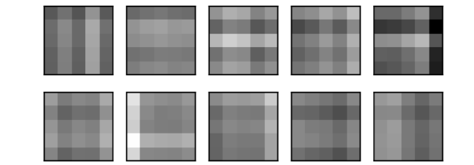
(a) Training data samples

(b) Learned generative fields

Figure 2: Artificial sparse bars dataset. (a) Example data which is constructed by Laplace-distributed activation of horizontal and vertical bars. (b) Optimizing $\mathcal{L}^{\mathcal{H}}$ recovers the bars and their activations (up to signs of generative fields).

4.2 Natural Image Patches, Sparsity and Entropy Annealing

After verification on artificial data, we investigated entropy-ELBOs using the presumably most standard application of sparse coding models: natural image patches. Learning sparse encodes for image patches based on Eq. 1 is also the most common approach to explain neuronal receptive fields in V1 cortex (Olshausen and Field, 1996). Originally estimated with MAP approximation, further extensions were developed to employ, e.g., VAE-style training with stochastic estimation of the ELBO gradient using the “reparameterization trick” (e.g. Barello et al., 2018; Tonolini et al., 2020). Here we used analytical entropy-ELBOs to optimize the model in Eq. 5 on whitened images (Olshausen and Field, 1996) with $N=204\,800$, $D=16\times 16$ and $H=100$ and $400$ (Section E.5 for experiments with $H=400$). We explored different versions of the entropy-ELBO, Eq. 15, in order to investigate the effect of entropy-based annealing and to compare it to amortized optimization. To allow for sufficient computational efficiency, we used variational distributions with diagonal or low-rank covariance matrices (see Eq. 159). Concretely, we used (A) an entropy-ELBO without annealing; (B) an entropy-ELBO (Eq. 160) with prior annealing ($\gamma\geq{}1$, $\delta=1$); (C) an entropy-ELBO using amortized variational distributions with diagonal covariance; and (D) the same amortized entropy-ELBO as in (C) but with low-rank approximation of the covariance matrices. For (A) and (B) we used EM-like updates: for every minibatch, we optimized variational parameters with L-BFGS and then took a gradient step to update $\tilde{W}$. For (C) and (D) neural networks were used to map data to means and (diagonal or low-rank) covariances, and for parameter optimization we used Adam-based gradient ascent provided by the standard PyTorch implementation (Paszke et al., 2017). For the annealed versions (B) and (D) we used prior annealing.

For all four different versions of entropy-ELBOs optimization ultimately resulted in the familiar Gabor-like generative fields: Figure 3 shows ELBO-optimization for the different versions, Section E.4 shows final GFs for $H=100$ and $H=400$. However, salient quantitative differences could be observed (see Fig. 3 and Fig. 4). Prior annealing of non-amortized entropy-ELBOs resulted in the fastest convergence and the highest ELBO values. Without annealing, non-amortized entropy-ELBOs finally resulted in very similar ELBO values but required longer to converge. Using also diagonal encoder covariances but amortized optimization, entropy-ELBOs converged more slowly and showed lower final ELBO values (see Fig. 3). Final ELBOs improved using low-rank covariance approximations and prior annealing (again Fig. 3). Low-rank covariances had a stronger effect on improvements (Wipf, 2023, for a related analysis) than prior annealing. In general, we observed that annealing has a comparably smaller effect for the amortized ELBO versions, which may be due to an interaction between annealing and standard Adam optimizers (Section E.3 for details).

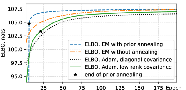
Figure 3: Optimization of entropy-ELBOs. Two non-amortized optimizations and two amortized optimizations are shown. Two optimizations use annealing.

Table 1: Different entropy annealings. No annealing (top), prior annealing (middle) and $\beta$-annealing (bottom) are compared (LABEL:{app:compare-annealing} for details).

ANNEALING		$\mathcal{H}[p_{\Theta}(\mathbf{z})]$	$\mathcal{H}[p_{\Theta}(\mathbf{x}|\mathbf{z})]$	$\mathcal{H}[q_{\Phi}(\mathbf{z})]$	ELBO	Gini$(\mathbf{z})\pm$SD
No annealing		32.40	-234.70	-98.97	103.33	$0.47\pm 0.04$
$\mathcal{H}[p_{\Theta}(\mathbf{z})]$	$\gamma=10.0$	-218.72	10.71	-365.22	-157.21	$0.59\pm 0.09$
	$\gamma=2.0$	-17.29	-144.81	-112.68	49.41	$0.58\pm 0.10$
	$\gamma=1.0$	29.65	-235.50	-99.67	106.18	$0.48\pm 0.05$
$\mathcal{H}[p_{\Theta}(\mathbf{x}|\mathbf{z})]$	$\delta=0.14$	-228.33	30.59	-234.02	-36.27	$0.55\pm 0.03$
	$\delta=0.50$	-17.77	-115.24	-72.77	60.24	$0.62\pm 0.04$
	$\delta=1.0$	29.74	-234.98	-99.43	105.80	$0.47\pm 0.05$

Next, we were interested in the different types of annealing suggested by entropy-ELBOs, see Eq. 17. Prior annealing ($\gamma\geq{}1$, $\delta=1$) very quickly resulted in a sparse encoding and localized GFs (see Fig. 4). This is consistent with the role of $\gamma$ in weighting a sparsity penalty term, see Eq. 18. Hence, it is prior annealing with $\gamma\geq{}1$ which is analogous to high weights for the sparsity penalty in $l_{1}$ sparse coding. That prior annealing results in sparser encodings is also confirmed when, e.g., using the Gini index (Hurley and Rickard, 2009) as a measure of sparsity (both Gini values and ELBO values are high, see Table 1). In contrast, $\beta$-annealing (used in $\beta$-VAEs), represents a type of regularization different from prior annealing resulting in much less localized GFs (LABEL:{app:compare-annealing} and Fig. 11).

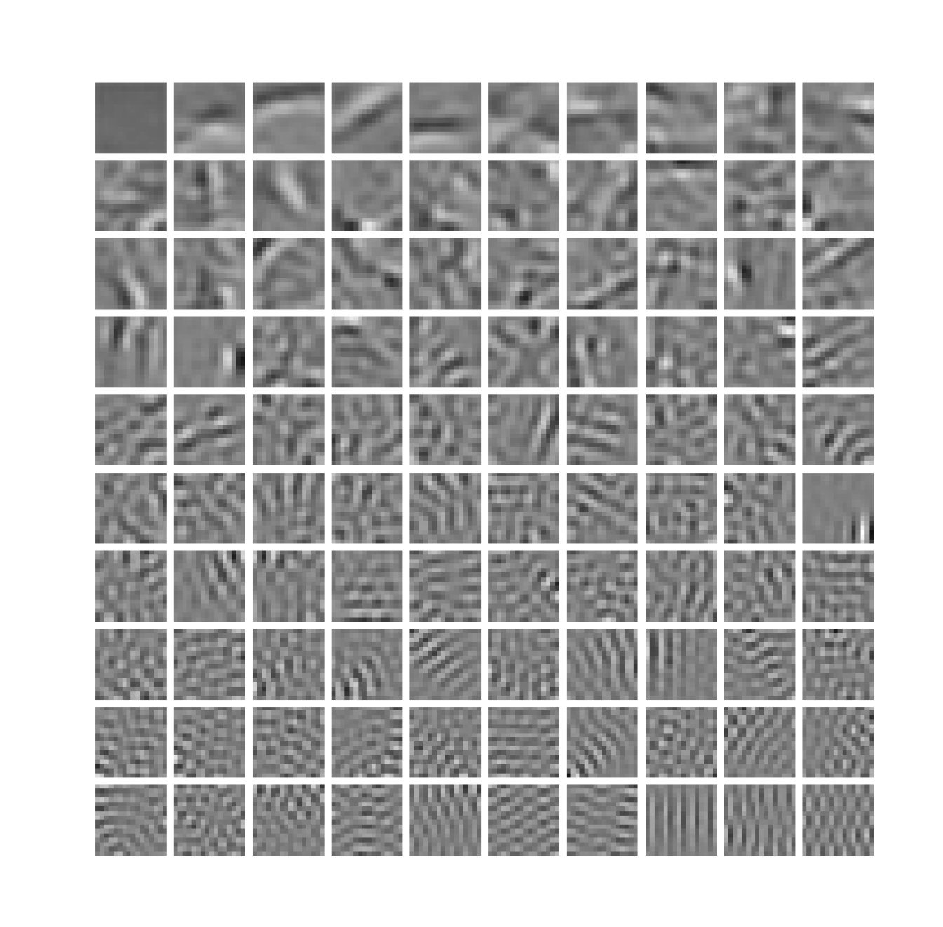
(a) No annealing, epoch 10

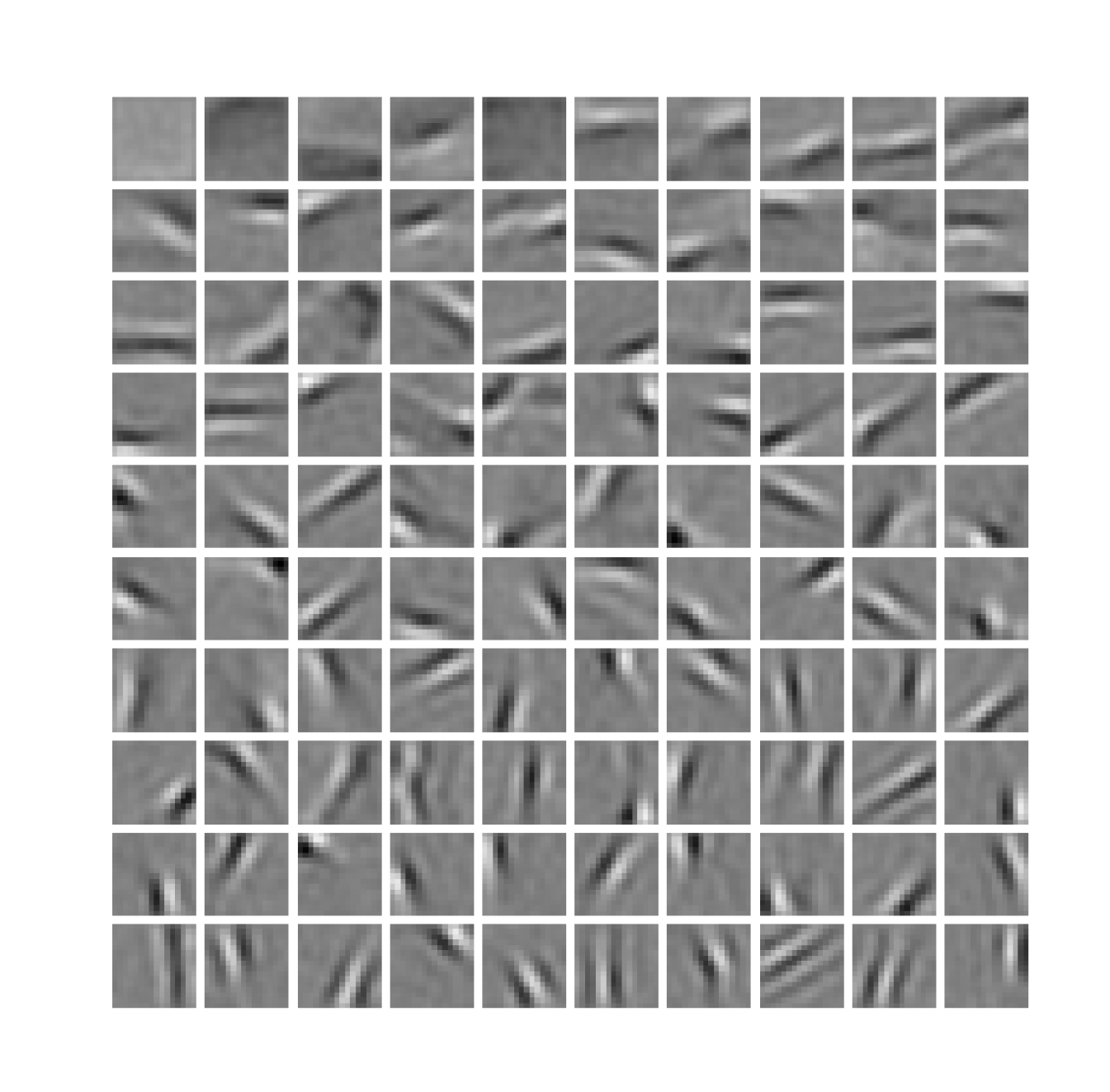
(b) Prior annealing, epoch 1

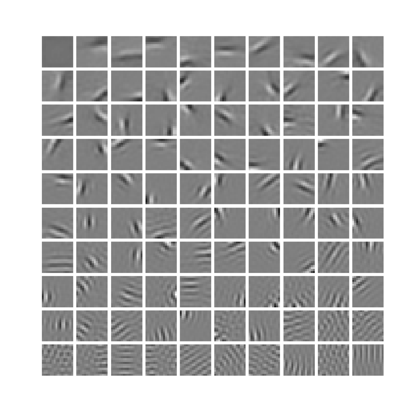
(c) Prior annealing, epoch 10

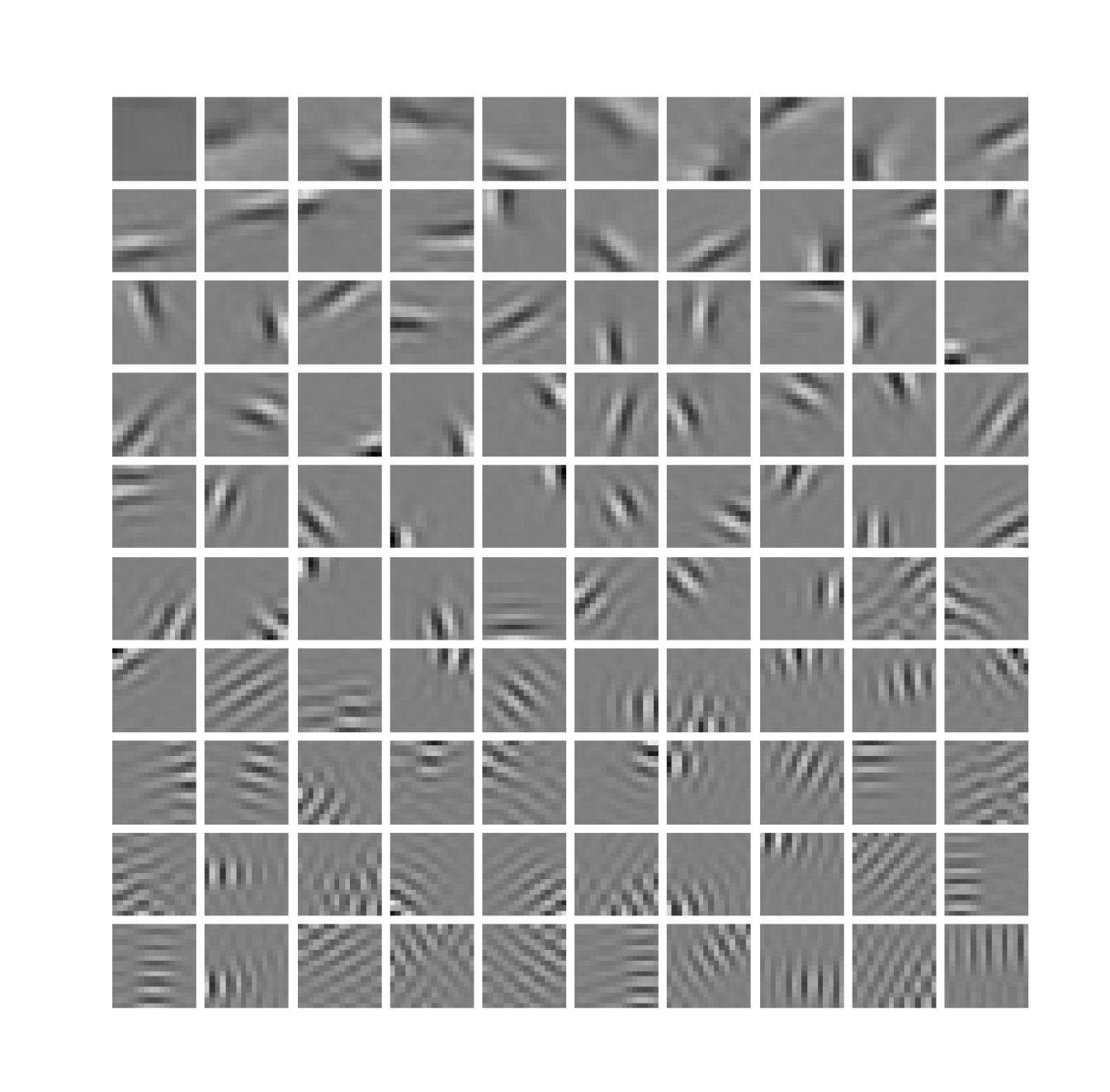
(d) Amortized, epoch 200

Figure 4: Learned generative fields on natural image patches. Without annealing, the convergence is slow (a). With the prior entropy annealing, even after one epoch, we observe classical localized Gabor filters (b). The final GFs (c) comprise a set of Gabors and higher frequency texture-like images. Learning with amortized posterior results in similar GFs (d).

Finally, our analytical objective also allows for easy estimation of ELBO values for sparse coding models optimized using standard MAP-based approaches. To show this, we used the original “sparsenet” code of Olshausen and Field (Olshausen, 1996). After optimization, we used the resulting $W$ matrix, normalized its columns, and optimized only the variational parameters of Gaussians (means and diagonal covariances). The obtained ELBO values of $94.719$ with Gini$(z)=0.464\pm 0.041$ indicates underfitting due to a manually selected weighting of the sparsity penalty.

5 DISCUSSION

Our main contributions are Theorems 1, 3 and 2. Taken together, these three theorems ensured that the here derived analytical objective in Eq. 15 can be used to optimize model parameters of standard probabilistic sparse coding. Apart from MAP-based approximations with known shortcomings for uncertainty encoding (cf. Section 1), there are many other approaches for sparse coding that maintain non-trivial posterior approximations. It could, of course, be argued that for those approaches at least the optimization algorithms (if not the objectives) are described by analytic or closed-form equations. Examples are the papers by Seeger (2008), who used expectation propagation to derive a learning algorithm, or by Berkes et al. (2007), who used Gaussian scale mixture ideas to facilitate variational optimization. The approach by Sheikh et al. (2014) also provides an analytical objective but at the cost of a combinatoric discrete optimization. In contrast to these and other previous approaches, we here remain with the most standard choices for probabilistic sparse coding. And it is for this setting, that we show the ELBO to have an analytical solution. Concretely, we remain (A) with the (by far) most standard model, Eq. 1; we use (B) the presumably most standard optimization framework (ELBOs for approximate maximum likelihood); and we use (C) the most standard posterior approximations (Gaussians). The here derived objective, presented in Eq. 15, then shows that all (high dimensional) integrals that emerge can be solved analytically. To the knowledge of the authors, this has previously not been shown or known. In this context it is noteworthy that analytical solutions for standard ELBOs could, in hindsight, also have been derived without knowledge of entropy convergence (we verified this observation in Section D.3).

Our results do, notably, apply very generally. Here, we have already numerically verified that potentially intricate deep neural networks (DNNs) can be used as encoders. The analytical objective then represents a deterministic DNN objective, and such objectives can conveniently be optimized with standard DNN tools. Equation 7 of Theorem 1 is still more general by applying for any decoder (linear or non-linear) with Gaussian observables. Theorem 1 thus extends to sparse VAEs which are of recent interest (Fallah and Rozell, 2022; Drefs et al., 2023; Chen et al., 2023). Future work can consequently investigate the here presented approaches like entropy annealing for such deep sparse coding models.

Conceptually maybe most relevantly, we here for the first time investigated how an ELBO objective can be reformulated as a solely entropy-based objective. From a theoretical perspective, entropies are more deeply rooted in the foundations of probabilistic machine learning, mathematical statistics, and information theory. Furthermore, for the class of distributions usually used to define generative models (exponential family, constant base measure), entropies are closed-form and are equipped with potentially convenient properties (via their log-partition function). Also, the derivatives of entropies, that are used for learning, have similarly convenient properties. Entropy convergence has previously only been considered for analysis (Lücke and Henniges, 2012; Damm et al., 2023), and, so far, it has been unclear if or how entropy convergence can be used for learning. In this work, we provided the first demonstration that solely entropy-based objectives can be used for learning, and there is no principled obstacle to extending this general approach to further generative models in the future.

Acknowledgments

This work is funded by the German Research Foundation (DFG) within the priority program SPP 2298 “Theoretical Foundations of Deep Learning” - project 464104047 (FI 2583/1-1 and LU 1196/9-1).

 

Learning Sparse Codes with Entropy-Based ELBOs:
Supplementary Materials

 

Appendix A PROOF OF THEOREM 3

Here, we lay out the details of the proof for Theorem 3. For completeness, we first restate the entropy-based ELBO (given equivalently in Eq. 15), which reads

$$\begin{split}\mathcal{L}^{\mathcal{H}}(\Phi,\tilde{W})=&\,\frac{1}{N}\sum_{n=1}^{N}\frac{1}{2}\log\big{(}\,|\,2\pi\,e\,\tau_{h}^{(n)}\,|\,\big{)}\\ &-\sum_{h=1}^{H}\log\Big{(}2\,e\,\frac{1}{N}\sum_{n=1}^{N}\tau_{h}^{(n)}{\cal M}\Big{(}\frac{\nu_{h}^{(n)}}{\tau_{h}^{(n)}}\Big{)}\Big{)}\\ &-\frac{D}{2}\log\Big{(}2\pi{}e\frac{1}{DN}\sum_{n=1}^{N}\operatorname{\mathbb{E}}_{q^{(n)}_{\Phi}\!(\mathbf{z})}\|\mathbf{x}^{(n)}-\tilde{W}\mathbf{z}\|^{2}\Big{)}\enspace,\end{split}$$

where we again use $\tau_{h}^{2}=\mathcal{T}_{hh}$ as a short-hand for the diagonal elements of the covariance (and $\tau_{h}=\sqrt{\mathcal{T}_{hh}}$ for their positive square root).

In order to prove Theorem 3 we rely on the following Lemma which establishes the equality of gradients on the manifold of optimal scales and variances, i.e., all points in parameter space that satisfy Eq. 6 for non-amortized and amortized parametrizations.

Lemma 1 (Equality of gradients on manifold of optimal scales and variance).

Consider the learning objectives $\mathcal{L}^{\mathrm{EL}}(\Phi,\Theta)$, given in Eq. 4, and $\mathcal{L}^{\mathcal{H}}(\Phi,\tilde{W})$, given in Eq. 15, for the probabilistic sparse coding model formulated in Eq. 5 with $\Theta=(\tilde{W},\sigma^{2},\boldsymbol{\lambda})\in\mathbb{R}_{\mathrm{norm}}^{D\times{}H}\times\mathbb{R}_{+}\times\mathbb{R}_{+}^{H}$, and variational parameters $\Phi=(\Phi_{\nu},\Phi_{\mathcal{T}})$ that parameterize mean $\boldsymbol{\nu}^{(n)}\in\mathbb{R}^{H}$ and covariance $\mathcal{T}^{(n)}\in\mathbb{R}^{H\times H}$ (in amortized or non-amortized fashion). We assume $\Phi_{\nu}\cap\Phi_{\mathcal{T}}=\emptyset$.

Then, whenever Eq. 6 holds, it holds that

$$\begin{split}\nabla_{\Phi}\mathcal{L}^{\mathrm{EL}}(\Phi,\Theta)&=\nabla_{\Phi}\mathcal{L}^{\mathcal{H}}(\Phi,\tilde{W})\enspace,\\ \nabla_{\tilde{W}}\mathcal{L}^{\mathrm{EL}}(\Phi,\Theta)&=\nabla_{\tilde{W}}\mathcal{L}^{\mathcal{H}}(\Phi,\tilde{W})\enspace.\end{split}$$ (19)

Proof.

We need to prove that the gradients for $\Theta$ and $\Phi$ for both objectives are equal at all points in parameter space whenever Eq. 6 is fulfilled, i.e., whenever the scales $\boldsymbol{\lambda}$ and the variance $\sigma^{2}$ are optimal.

Recall that the ELBO, given in Eq. 4, can be written as (using the notation of Theorem 1)

$$\mathcal{L}^{\mathrm{EL}}(\Phi,\Theta)=\overbrace{\frac{1}{N}\sum_{n=1}^{N}\mathcal{H}[q_{\Phi}^{(n)}(\mathbf{z})]+\mathcal{L}^{\mathrm{EL}}_{1}(\Phi,\Theta)}^{\text{regularization (neg. KL-divergence)}}\overbrace{+\vphantom{\frac{1}{N}\sum_{n=1}^{N}}\mathcal{L}^{\mathrm{EL}}_{2}(\Phi,\Theta)}^{\text{reconstruction}}$$ (20)

and whenever the condition of Theorem 1 (i.e., Eq. 6) is satisfied, we observe the term-wise convergence to entropies such that the ELBO decomposes into three entropies

$$=\underbrace{\frac{1}{N}\sum_{n=1}^{N}\mathcal{H}[q_{\Phi}^{(n)}(\mathbf{z})]-\mathcal{H}[p_{\Theta}(\mathbf{z})]}_{\text{regularization (neg. KL-divergence)}}\underbrace{-\vphantom{\frac{1}{N}\sum_{n=1}^{N}}\mathcal{H}[p_{\Theta}(\mathbf{x}|\mathbf{z})]}_{\text{reconstruction}}\enspace.$$ (21)

Note that the entropy-based objective $\mathcal{L}^{\mathcal{H}}$, given in Eq. 15, is merely the sum of entropies above with analytically optimal scale and variance parameters obtained from Theorem 2.

We need to investigate the gradients with respect to the parameters of the model $\Theta=(\tilde{W},\sigma^{2},\boldsymbol{\lambda})$ and the variational parameters $\Phi=(\Phi_{\nu},\Phi_{\mathcal{T}})$. We start by addressing the model parameters $\Theta$.

Model Parameters $\Theta$: Considering $\Theta$, only the parameters $w\in\tilde{W}$ are of interest. Thus, only the reconstruction terms, $\mathcal{L}^{\mathrm{EL}}_{2}$ and its counterpart $-\mathcal{H}[p_{\Theta}(\mathbf{x}|\mathbf{z})]$, contribute to the gradients for $\tilde{W}$. We consider a general parameter $w\in\tilde{W}$. Regarding the standard ELBO $\mathcal{L}^{\mathrm{EL}}$, the gradient is given by

$$\frac{\partial}{\partial w}\mathcal{L}^{\mathrm{EL}}(\Phi,\Theta) =\frac{\partial}{\partial w}\mathcal{L}^{\mathrm{EL}}_{2}(\Theta,\Phi)$$ (22)

$$=-\frac{1}{2\sigma^{2}}\frac{\partial}{\partial w}\left[\frac{1}{N}\sum_{n=1}^{N}\operatorname{\mathbb{E}}_{q^{(n)}_{\Phi}(\mathbf{z})}\big{\|}\mathbf{x}^{(n)}-\tilde{W}\mathbf{z}\big{\|}^{2}\right]$$ (23)

$$=-\frac{1}{\sigma^{2}}\frac{1}{N}\sum_{n=1}^{N}\operatorname{\mathbb{E}}_{q^{(n)}_{\Phi}(\mathbf{z})}\left(\mathbf{x}^{(n)}-\tilde{W}\mathbf{z}\right)\frac{\partial}{\partial w}\tilde{W}\mathbf{z}\enspace.$$ (24)

Similarly, for the entropy-based ELBO $$\mathcal{L}^{\mathcal{H}}$$ we obtain

$$\frac{\partial}{\partial w}\mathcal{L}^{\mathcal{H}}(\Phi,\tilde{W}) =-\frac{\partial}{\partial w}\mathcal{H}[p_{\Theta}(\mathbf{x}|\mathbf{z})]$$ (25)

$$=-\frac{D}{2}\frac{\partial}{\partial w}\log\big{(}2\pi e\frac{1}{ND}\sum_{n=1}^{N}\operatorname{\mathbb{E}}_{q^{(n)}_{\Phi}(\mathbf{z})}\big{\|}\mathbf{x}^{(n)}-\tilde{W}\mathbf{z}\big{\|}^{2}\big{)}$$ (26)

$$=-D\frac{\frac{1}{N}\sum_{n=1}^{N}\operatorname{\mathbb{E}}_{q^{(n)}_{\Phi}(\mathbf{z})}\left(\mathbf{x}^{(n)}-\tilde{W}\mathbf{z}\right)}{\frac{1}{N}\sum_{n=1}^{N}\operatorname{\mathbb{E}}_{q^{(n)}_{\Phi}(\mathbf{z})}\big{\|}\mathbf{x}^{(n)}-\tilde{W}\mathbf{z}\big{\|}^{2}}\frac{\partial}{\partial w}\tilde{W}\mathbf{z}\enspace,$$ (27)

and with $$\sigma^{2}_{\mathrm{opt}}(\Phi,\tilde{W})=\frac{1}{ND}\sum_{n=1}^{N}\operatorname{\mathbb{E}}_{q^{(n)}_{\Phi}(\mathbf{z})}\big{\|}\mathbf{x}^{(n)}-\tilde{W}\mathbf{z}\big{\|}^{2}$$ (as derived in Theorem 2) we conclude

$$=-\frac{1}{\sigma^{2}_{\mathrm{opt}}}\frac{1}{N}\sum_{n=1}^{N}\operatorname{\mathbb{E}}_{q^{(n)}_{\Phi}(\mathbf{z})}\left(\mathbf{x}^{(n)}-\tilde{W}\mathbf{z}\right)\frac{\partial}{\partial w}\tilde{W}\mathbf{z}\enspace.$$ (28)

Observe that both objectives yield the same gradient information for any $w\in\tilde{W}$, just scaled by a ratio that reflects how far $\sigma^{2}$ is from its optimal value $\sigma^{2}_{\mathrm{opt}}$, such that

$$\nabla_{\tilde{W}}\mathcal{L}^{\mathcal{H}}(\Phi,\tilde{W})=\frac{\sigma^{2}}{\sigma^{2}_{\mathrm{opt}}}\nabla_{\tilde{W}}\mathcal{L}^{\mathrm{EL}}(\Phi,(\boldsymbol{\lambda},\tilde{W},\sigma^{2}))\enspace.$$ (29)

Importantly, both objectives give rise to the same gradients for $\tilde{W}$ whenever $\sigma^{2}=\sigma^{2}_{\mathrm{opt}}$, i.e., when Eq. 6 is satisfied.

Variational Parameters $\Phi$: It remains to investigate how the gradients for the variational parameters $\Phi$ are affected when training with $\mathcal{L}^{\mathrm{EL}}$ or $\mathcal{L}^{\mathcal{H}}$. We consider $\phi\in\Phi$ for which the gradient decomposes into three terms

$$\frac{\partial}{\partial\phi}\mathcal{L}^{\mathrm{EL}}(\Phi,\Theta) =\frac{\partial}{\partial\phi}\frac{1}{N}\sum_{n=1}^{N}\mathcal{H}[q_{\Phi}^{(n)}(\mathbf{z})]+\frac{\partial}{\partial\phi}\mathcal{L}^{\mathrm{EL}}_{1}(\Phi,\Theta)+\frac{\partial}{\partial\phi}\sum_{n=1}^{N}\mathcal{L}^{\mathrm{EL}}_{2}(\Phi,\Theta),$$ (30)

$$\frac{\partial}{\partial\phi}\mathcal{L}^{\mathcal{H}}(\Phi,\tilde{W}) =\frac{\partial}{\partial\phi}\frac{1}{N}\sum_{n=1}^{N}\mathcal{H}[q_{\Phi}^{(n)}(\mathbf{z})]-\frac{\partial}{\partial\phi}\mathcal{H}[p_{\Theta}(\mathbf{z})]-\frac{\partial}{\partial\phi}\mathcal{H}[p_{\Theta}(\mathbf{x}|\mathbf{z})]$$ (31)

The average encoder entropy (the first term in Eqs. 31 and 30, respectively) is part of both objectives and consequently provides the same gradient information for any $\phi\in\Phi$ (regardless of the concrete parametrization in terms of $\Phi$). We continue with the gradient updates arising from the reconstruction score, i.e., $\mathcal{L}^{\mathrm{EL}}_{2}(\Phi,\Theta)$ vs. $-\mathcal{H}[p_{\Theta}(\mathbf{x}|\mathbf{z})]$, the last term in Eqs. 31 and 30, respectively. Starting with the latter we get

$$-\frac{\partial}{\partial\phi}\mathcal{H}[p_{\Theta}(\mathbf{x}|\mathbf{z})] =-\frac{D}{2}\frac{\partial}{\partial\phi}\log\big{(}2\pi e\sigma^{2}_{\mathrm{opt}}(\Phi,\tilde{W})\big{)}$$ (32)

$$=-\frac{D}{2}\frac{1}{\sigma^{2}_{\mathrm{opt}}(\Phi,\tilde{W})}\frac{\partial}{\partial\phi}\sigma^{2}_{\mathrm{opt}}(\Phi,\tilde{W})$$ (33)

and by invoking $$\sigma^{2}_{\mathrm{opt}}(\Phi,\tilde{W})=\frac{1}{ND}\sum_{n=1}^{N}\operatorname{\mathbb{E}}_{q_{\Phi}(\mathbf{z}|\mathbf{x}^{(n)})}\big{\|}\mathbf{x}^{(n)}-\tilde{W}\mathbf{z})\big{\|}^{2}$$,

$$=-\frac{1}{2\sigma^{2}_{\mathrm{opt}}}\frac{\partial}{\partial\phi}\left[\frac{1}{N}\sum_{n=1}^{N}\operatorname{\mathbb{E}}_{q(\mathbf{z}|\mathbf{x}^{(n)})}\big{\|}\mathbf{x}^{(n)}-\tilde{W}\mathbf{z}\big{\|}^{2}\right]\enspace.$$ (34)

Considering the corresponding counterpart, $\mathcal{L}^{\mathrm{EL}}_{2}(\Phi,\Theta)$ in the classical ELBO, the gradient is directly given by

$$\frac{\partial}{\partial\phi}\mathcal{L}^{\mathrm{EL}}_{2}(\Phi,\Theta) =-\frac{1}{2\sigma^{2}}\frac{\partial}{\partial\phi}\left[\frac{1}{N}\sum_{n=1}^{N}\operatorname{\mathbb{E}}_{q(\mathbf{z}|\mathbf{x}^{(n)})}\big{\|}\mathbf{x}^{(n)}-\tilde{W}\mathbf{z}\big{\|}^{2}\right]\enspace,$$ (35)

such that gradient updates are again scaled depending on how close $\sigma^{2}$ is to $\sigma^{2}_{\mathrm{opt}}$

$$-\frac{\partial}{\partial\phi}\mathcal{H}[p_{\Theta}(\mathbf{x}|\mathbf{z})]=\frac{\sigma^{2}}{\sigma^{2}_{\mathrm{opt}}}\frac{\partial}{\partial\phi}\mathcal{L}^{\mathrm{EL}}_{2}(\Phi,\Theta)\enspace.$$ (36)

We are left with the middle terms in Eqs. 30 and 31, i.e., $\frac{\partial}{\partial\phi}\mathcal{L}^{\mathrm{EL}}_{1}(\Phi,\Theta)$ vs. $-\frac{\partial}{\partial\phi}\mathcal{H}[p_{\Theta}(\mathbf{z})]$. To enable the gradient computations we first need to derive a closed-form expression for $\mathcal{L}^{\mathrm{EL}}_{1}(\Phi,\Theta)$ with $q_{\Phi}^{(n)}(\mathbf{z})=\mathcal{N}(\mathbf{z};\boldsymbol{\nu}^{(n)},\mathcal{T}^{(n)}\big{)}$, again with diagonal elements $\tau_{h}^{2}=\mathcal{T}_{hh}$, and a Laplace prior with learnable scales $\lambda_{h}$, i.e., $p_{\Theta}(\mathbf{\mathbf{z}})=\prod_{h=1}^{H}\frac{1}{2\lambda_{h}}\exp\left(-\frac{|z_{h}|}{\lambda_{h}}\right)$.

Recall that $\mathcal{L}^{\mathrm{EL}}_{1}(\Phi,\Theta)=\textstyle\frac{1}{N}\sum_{n}\int q^{(n)}_{\Phi}(\mathbf{z})\log p_{\Theta}(\mathbf{z})\mathrm{d}\mathbf{z}$ for which the individual summands evaluate to

$$\int q_{\Phi}^{(n)}(\mathbf{z})\log p_{\Theta}(\mathbf{z})\mathrm{d}\mathbf{z} =\int\mathcal{N}(\mathbf{z}|\boldsymbol{\nu}^{(n)},\mathcal{T}^{(n)})\Big{(}\sum_{h=1}^{H}\log\Big{(}\frac{1}{2\lambda_{h}}\Big{)}-\sum_{h=1}\frac{|z_{h}|}{\lambda_{h}}\Big{)}\mathrm{d}\mathbf{z}$$ (37)

$$=\sum_{h=1}^{H}\log\Big{(}\frac{1}{2\lambda_{h}}\Big{)}-\int\mathcal{N}(\mathbf{z}|\boldsymbol{\nu}^{(n)},\mathcal{T}^{(n)})\sum_{h=1}\frac{|z_{h}|}{\lambda_{h}}\mathrm{d}\mathbf{z}$$ (38)

$$=-\sum_{h=1}^{H}\log(2\lambda_{h})-\sum_{h=1}^{H}\frac{1}{\lambda_{h}}\int\mathcal{N}(z_{h}|\nu^{(n)}_{h},\mathcal{T}^{(n)}_{hh})|z_{h}|\mathrm{d}z_{h}$$ (39)

$$=-\sum_{h=1}^{H}\log(2\lambda_{h})-\sum_{h=1}^{H}\frac{1}{\lambda_{h}}\left[\sqrt{\frac{2}{\pi}}\tau_{h}^{(n)}\exp\left(-\frac{1}{2}\Bigg{(}\frac{\nu_{h}^{(n)}}{\tau_{h}^{(n)}}\Bigg{)}^{2}\right)+\nu_{h}^{(n)}\operatorname{erf}\left(\frac{\nu_{h}^{(n)}}{\sqrt{2}\tau_{h}^{(n)}}\right)\right]\enspace.$$ (40)

With help of the statistic $${\cal M}(a)=\sqrt{\frac{2}{\pi}}\exp\left(-\frac{1}{2}\,a^{2}\right)+a\operatorname{erf}\left(\frac{a}{\sqrt{2}}\right)$$, introduced in Eq. 12, we get

$$=-\sum_{h=1}^{H}\log(2\lambda_{h})-\sum_{h=1}^{H}\frac{\tau_{h}^{(n)}}{\lambda_{h}}\mathcal{M}\Big{(}\frac{\nu_{h}^{(n)}}{\tau_{h}^{(n)}}\Big{)}$$ (41)

such that

$$\mathcal{L}^{\mathrm{EL}}_{1}(\Phi,\Theta) =-\frac{1}{N}\sum_{n=1}^{N}\sum_{h=1}^{H}\left[\log(\lambda_{h})+\frac{\tau_{h}^{(n)}}{\lambda_{h}}\mathcal{M}\Big{(}\frac{\nu_{h}^{(n)}}{\tau_{h}^{(n)}}\Big{)}+c\right]$$ (42)

for some constant $c$ (that does not influence any gradients). Note that now the functional dependency for mean and variance parameters matters for the gradient calculations, such that we need to consider $\phi\in\Phi_{\nu}$ and $\phi\in\Phi_{\mathcal{T}}$ separately.

Before proceeding we need to address the different parametrization that arises for non-amortized vs. amortized approaches. In the non-amortized setting, the variational parameters $\Phi=(\Phi_{\nu},\Phi_{\mathcal{T}})$ directly parameterize mean and covariance of $q_{\Phi}^{(n)}$ (per data point $\mathbf{x}^{(n)}$), i.e., $\Phi_{\nu}=(\boldsymbol{\nu}^{(1)},\ldots,\boldsymbol{\nu}^{(N)})$ and $\Phi_{\mathcal{T}}=(\mathcal{T}^{(1)},\ldots,\mathcal{T}^{(N)})$. In amortized approaches, we take $\Phi=(\Phi_{\nu},\Phi_{\mathcal{T}})$ to parameterize the two functions $\boldsymbol{\nu}_{\Phi}:\mathbb{R}^{D}\to\mathbb{R}^{H}$ and $\mathcal{T}_{\Phi}:\mathbb{R}^{D}\to\mathbb{R}^{H\times H}$ such that mean and covariance are given as the respective function outputs, i.e,

$$\boldsymbol{\nu}^{(n)} =\boldsymbol{\nu}_{\Phi}(\mathbf{x}^{(n)})\enspace,$$ (43)

$$\mathcal{T}^{(n)} =\mathcal{T}_{\Phi}(\mathbf{x}^{(n)})\enspace.$$ (44)

The derivations in the sequel cover both settings, as we only need to compare the resulting gradients in terms of functions of partial derivatives $\frac{\partial\nu_{h}^{(n)}}{\partial\phi_{\nu}}$ or $\frac{\partial\tau_{h}^{(n)}}{\partial\phi_{\tau}}$, which clearly differ in amortized vs. non-amortized parametrizations, but are the same for both objectives.

Variational Parameters: Mean

Let us continue with the gradient updates for the variational mean $\boldsymbol{\nu}_{\Phi}$, so just the mean parameters $\phi_{\nu}\in\Phi_{\nu}$ are of interest here. Considering $\mathcal{L}^{\mathrm{EL}}$ first, the updates for $\boldsymbol{\nu}$ from $\mathcal{L}^{\mathrm{EL}}_{1}(\Phi,\Theta)$, in the form of Eq. 42, result in

$$\frac{\partial}{\partial\phi_{\nu}}\mathcal{L}^{\mathrm{EL}}_{1}(\Phi,\Theta) =-\frac{1}{N}\sum_{n=1}^{N}\sum_{h=1}^{H}\frac{\tau_{h}^{(n)}}{\lambda_{h}}\frac{\partial}{\partial\phi_{\nu}}\mathcal{M}\Big{(}\frac{\nu_{h}^{(n)}}{\tau_{h}^{(n)}}\Big{)}$$ (45)

$$=-\frac{1}{N}\sum_{n=1}^{N}\sum_{h=1}^{H}\frac{1}{\lambda_{h}}\operatorname{erf}\Big{(}\frac{1}{\sqrt{2}}\frac{\nu_{h}^{(n)}}{\tau_{h}^{(n)}}\Big{)}\frac{\partial\nu_{h}^{(n)}}{\partial\phi_{\nu}}\enspace,$$ (46)

where we made use of the following derivative which invokes the fact that $$\frac{\partial\mathcal{M}(a)}{\partial a}=\operatorname{erf}\left(\frac{a}{\sqrt{2}}\right)$$,

$$\frac{\partial}{\partial\phi_{\nu}}\mathcal{M}\Big{(}\frac{\nu_{h}^{(n)}}{\tau_{h}^{(n)}}\Big{)} =\frac{1}{\tau_{h}^{(n)}}\operatorname{erf}\Big{(}\frac{1}{\sqrt{2}}\frac{\nu_{h}^{(n)}}{\tau_{h}^{(n)}}\Big{)}\frac{\partial\nu_{h}^{(n)}}{\partial\phi_{\nu}}\enspace.$$ (47)

Now, the respective gradient updates from the prior entropy of the entropy-based objective $\mathcal{L}^{\mathcal{H}}$ are given as

$$-\frac{\partial}{\partial\phi_{\nu}}\mathcal{H}[p_{\Theta}(\mathbf{z})] =-\frac{\partial}{\partial\phi_{\nu}}\sum_{h=1}^{H}\log(2e\lambda_{\mathrm{opt},h}(\Phi))$$ (48)

$$=-\sum_{h=1}^{H}\frac{1}{\lambda_{\mathrm{opt},h}}\frac{\partial}{\partial\phi_{\nu}}\lambda_{\mathrm{opt},h}(\Phi)$$ (49)

$$=-\frac{1}{N}\sum_{n=1}^{N}\sum_{h=1}^{H}\frac{1}{\lambda_{\mathrm{opt},h}(\Phi)}\operatorname{erf}\Big{(}\frac{1}{\sqrt{2}}\frac{\nu_{h}^{(n)}}{\tau_{h}^{(n)}}\Big{)}\frac{\partial\nu_{h}^{(n)}}{\partial\phi_{\nu}}\enspace.$$ (50)

The line above makes use of the following derivation

$$\frac{\partial}{\partial\phi_{\nu}}\lambda_{\mathrm{opt},h}(\Phi) =\frac{\partial}{\partial\phi_{\nu}}\frac{1}{N}\sum_{n=1}^{N}\tau_{h}^{(n)}\mathcal{M}\Big{(}\frac{\nu_{h}^{(n)}}{\tau_{h}^{(n)}}\Big{)}$$ (51)

$$=\frac{1}{N}\sum_{n=1}^{N}\frac{\tau_{h}^{(n)}}{\tau_{h}^{(n)}}\operatorname{erf}\Big{(}\frac{1}{\sqrt{2}}\frac{\nu_{h}^{(n)}}{\tau_{h}^{(n)}}\Big{)}\frac{\partial\nu_{h}^{(n)}}{\partial\phi_{\nu}}$$ (52)

$$=\frac{1}{N}\sum_{n=1}^{N}\operatorname{erf}\Big{(}\frac{1}{\sqrt{2}}\frac{\nu_{h}^{(n)}}{\tau_{h}^{(n)}}\Big{)}\frac{\partial\nu_{h}^{(n)}}{\partial\phi_{\nu}}\enspace.$$ (53)

By comparing Eqs. 46 and 50 we again conclude that the gradients just differ in the scaling by $1/\lambda_{h}$ vs. $1/\lambda_{\mathrm{opt},h}$. That is, for optimal scales $\boldsymbol{\lambda}=\boldsymbol{\lambda}_{\mathrm{opt}}$ the gradients of the regularization term for the variational mean $\boldsymbol{\nu}$ coincide.

Variational Parameters: Variance

A similar result holds for (the parameters of) the variational variances. We consider $\phi_{\tau}\in\Phi_{\mathcal{T}}$ and start with the prior entropy in $\mathcal{L}^{\mathcal{H}}$. The gradient w.r.t. $\phi_{\tau}$ reads

$$-\frac{\partial}{\partial\phi_{\tau}}\mathcal{H}[p_{\Theta}(\mathbf{z})] =-\frac{\partial}{\partial\phi_{\tau}}\sum_{h=1}^{H}\log(2e\lambda_{\mathrm{opt},h}(\Phi))$$ (54)

$${=}-\frac{\partial}{\partial\phi_{\tau}}\sum_{h=1}^{H}\log\Bigg{(}2e\frac{1}{N}\sum_{n=1}^{N}\tau_{h}^{(n)}\mathcal{M}\Big{(}\frac{\nu_{h}^{(n)}}{\tau_{h}^{(n)}}\Big{)}\Bigg{)}$$ (55)

$$=-\sum_{h=1}^{H}\frac{1}{\lambda_{\mathrm{opt},h}(\Phi)}\frac{\partial}{\partial\phi_{\tau}}\Bigg{(}\frac{1}{N}\sum_{n=1}^{N}\tau_{h}^{(n)}\mathcal{M}\Big{(}\frac{\nu_{h}^{(n)}}{\tau_{h}^{(n)}}\Big{)}\Bigg{)}$$ (56)

$$=-\frac{1}{N}\sum_{n=1}^{N}\sum_{h=1}^{H}\frac{1}{\lambda_{\mathrm{opt},h}(\Phi)}\sqrt{\frac{2}{\pi}}\exp\Big{(}-\frac{1}{2}\frac{\nu_{h}^{(n)}}{\tau_{h}^{(n)}}\Big{)}\frac{\partial\tau_{h}^{(n)}}{\partial\phi_{\tau}}\enspace,$$ (57)

where the last line makes use of the following derivation

$$\frac{\partial}{\partial\phi_{\tau}}\Bigg{(}\frac{1}{N}\sum_{n=1}^{N}\tau_{h}^{(n)}\mathcal{M}\Big{(}\frac{\nu_{h}^{(n)}}{\tau_{h}^{(n)}}\Big{)}\Bigg{)} =\frac{1}{N}\sum_{n=1}^{N}\left[\mathcal{M}\Big{(}\frac{\nu_{h}^{(n)}}{\tau_{h}^{(n)}}\Big{)}\frac{\partial\tau_{h}^{(n)}}{\partial\phi_{\tau}}+\tau_{h}^{(n)}\frac{\partial}{\partial\phi_{\tau}}\mathcal{M}\Big{(}\frac{\nu_{h}^{(n)}}{\tau_{h}^{(n)}}\Big{)}\right]$$ (58)

$$=\frac{1}{N}\sum_{n=1}^{N}\left[\mathcal{M}\Big{(}\frac{\nu_{h}^{(n)}}{\tau_{h}^{(n)}}\Big{)}-\frac{\nu_{h}^{(n)}}{\tau_{h}^{(n)}}\operatorname{erf}\Big{(}\frac{1}{\sqrt{2}}\frac{\nu_{h}^{(n)}}{\tau_{h}^{(n)}}\Big{)}\right]\frac{\partial\tau_{h}^{(n)}}{\partial\phi_{\tau}}$$ (59)

$${=}\frac{1}{N}\sum_{n=1}^{N}\sqrt{\frac{2}{\pi}}\exp\Big{(}-\frac{1}{2}\frac{\nu_{h}^{(n)}}{\tau_{h}^{(n)}}\Big{)}\frac{\partial\tau_{h}^{(n)}}{\partial\phi_{\tau}}\enspace.$$ (60)

Lastly, for $\mathcal{L}^{\mathrm{EL}}$ we consider the remaining term $\mathcal{L}^{\mathrm{EL}}_{1}(\Phi)$ which gradients evaluate to

$$\frac{\partial}{\partial\phi_{\tau}}\mathcal{L}^{\mathrm{EL}}_{1}(\Phi) =-\frac{\partial}{\partial\phi_{\tau}}\frac{1}{N}\sum_{n=1}^{N}\sum_{h=1}^{H}\left[\log(\lambda_{h})+\frac{\tau_{h}^{(n)}}{\lambda_{h}}\mathcal{M}\Big{(}\frac{\nu_{h}^{(n)}}{\tau_{h}^{(n)}}\Big{)}+c\right]$$ (61)

$$=-\frac{\partial}{\partial\phi_{\tau}}\frac{1}{N}\sum_{n=1}^{N}\sum_{h=1}^{H}\left[\frac{\tau_{h}^{(n)}}{\lambda_{h}}\mathcal{M}\Big{(}\frac{\nu_{h}^{(n)}}{\tau_{h}^{(n)}}\Big{)}\right]$$ (62)

and with the derivations in Eq. 58 – Eq. 60 we get

$$=-\frac{1}{N}\sum_{n=1}^{N}\sum_{h=1}^{H}\frac{1}{\lambda_{h}}\sqrt{\frac{2}{\pi}}\exp\Big{(}-\frac{1}{2}\frac{\nu_{h}^{(n)}}{\tau_{h}^{(n)}}\Big{)}\frac{\partial\tau_{h}^{(n)}}{\partial\phi_{\tau}}\enspace.$$ (63)

Again, the resulting gradients in Eqs. 63 and 57 just differ in the scaling $1/\lambda_{h}$ vs. $1/\lambda_{\mathrm{opt},h}$.

Note that Theorem 3 can be generalized to allow for parameter sharing, i.e., the additional assumption $\Phi_{\nu}\cap\Phi_{\mathcal{T}}=\emptyset$ can be dropped. However, we invoked this additional assumption as it (slightly) simplifies and shortens the equations and the overall proof. With the assumption $\Phi_{\nu}\cap\Phi_{\mathcal{T}}=\emptyset$, we can now summarize the term-wise gradient calculations by completing Eqs. 30 and 31

$$\frac{\partial}{\partial\phi}\mathcal{L}^{\mathrm{EL}}(\Phi,\Theta) =\frac{\partial}{\partial\phi}\frac{1}{N}\sum_{n=1}^{N}\mathcal{H}[q_{\Phi}^{(n)}(\mathbf{z})]+\frac{\partial}{\partial\phi}\mathcal{L}^{\mathrm{EL}}_{1}(\Phi,\Theta)+\frac{\partial}{\partial\phi}\sum_{n=1}^{N}\mathcal{L}^{\mathrm{EL}}_{2}(\Phi,\Theta)$$

$$\begin{split}&=\frac{\partial}{\partial\phi}\frac{1}{N}\sum_{n=1}^{N}\mathcal{H}[q_{\Phi}^{(n)}(\mathbf{z})]-\frac{1}{N}\sum_{n=1}^{N}\sum_{h=1}^{H}{\color[rgb]{0.859375,0.1875,0.4765625}\frac{1}{\lambda_{h}}}\operatorname{erf}\Big{(}\frac{1}{\sqrt{2}}\frac{\nu_{h}^{(n)}}{\tau_{h}^{(n)}}\Big{)}\frac{\partial\nu_{h}^{(n)}}{\partial\phi}\\ &\hskip 14.22636pt-\frac{1}{N}\sum_{n=1}^{N}\sum_{h=1}^{H}{\color[rgb]{0.859375,0.1875,0.4765625}\frac{1}{\lambda_{h}}}\sqrt{\frac{2}{\pi}}\exp\Big{(}-\frac{1}{2}\frac{\nu_{h}^{(n)}}{\tau_{h}^{(n)}}\Big{)}\frac{\partial\tau_{h}^{(n)}}{\partial\phi}-{\color[rgb]{0.859375,0.1875,0.4765625}\frac{1}{2\sigma^{2}}}\frac{\partial}{\partial\phi}\left[\frac{1}{N}\sum_{n=1}^{N}\operatorname{\mathbb{E}}_{q(\mathbf{z}|\mathbf{x}^{(n)})}\big{\|}\mathbf{x}^{(n)}-\tilde{W}\mathbf{z}\big{\|}^{2}\right]\enspace,\end{split}$$ (64)

$$\frac{\partial}{\partial\phi}\mathcal{L}^{\mathcal{H}}(\Phi,\tilde{W}) =\frac{\partial}{\partial\phi}\frac{1}{N}\sum_{n=1}^{N}\mathcal{H}[q_{\Phi}^{(n)}(\mathbf{z})]-\frac{\partial}{\partial\phi}\mathcal{H}[p_{\Theta}(\mathbf{z})]-\frac{\partial}{\partial\phi}\mathcal{H}[p_{\Theta}(\mathbf{x}|\mathbf{z})]$$

$$\begin{split}&=\frac{\partial}{\partial\phi}\frac{1}{N}\sum_{n=1}^{N}\mathcal{H}[q_{\Phi}^{(n)}(\mathbf{z})]-\frac{1}{N}\sum_{n=1}^{N}\sum_{h=1}^{H}{\color[rgb]{0.859375,0.1875,0.4765625}\frac{1}{\lambda_{\mathrm{opt},h}(\Phi)}}\operatorname{erf}\Big{(}\frac{1}{\sqrt{2}}\frac{\nu_{h}^{(n)}}{\tau_{h}^{(n)}}\Big{)}\frac{\partial\nu_{h}^{(n)}}{\partial\phi}\\ &-\frac{1}{N}\sum_{n=1}^{N}\sum_{h=1}^{H}{\color[rgb]{0.859375,0.1875,0.4765625}\frac{1}{\lambda_{\mathrm{opt},h}(\Phi)}}\sqrt{\frac{2}{\pi}}\exp\Big{(}-\frac{1}{2}\frac{\nu_{h}^{(n)}}{\tau_{h}^{(n)}}\Big{)}\frac{\partial\tau_{h}^{(n)}}{\partial\phi}-{\color[rgb]{0.859375,0.1875,0.4765625}\frac{1}{2\sigma^{2}_{\mathrm{opt}}}}\frac{\partial}{\partial\phi}\left[\frac{1}{N}\sum_{n=1}^{N}\operatorname{\mathbb{E}}_{q(\mathbf{z}|\mathbf{x}^{(n)})}\big{\|}\mathbf{x}^{(n)}-\tilde{W}\mathbf{z}\big{\|}^{2}\right]\enspace.\end{split}$$ (65)

Overall, at points in parameter space that satisfy Eq. 6, each pair of terms gives rise to the same gradients at stationary points as all scaling coefficients (highlighted in light red) coincide (or the respective terms already provide the very same gradient information regardless of whether Eq. 6 is satisfied). Consequently, the full gradients for all trainable parameters, i.e., the sum of all constitutive terms as given in Eqs. 64 and 65 for $\Phi$ and Eq. 29 for $\tilde{W}$, are equivalent whenever Eq. 6 holds, or simply: Eq. 6 implies

$$\nabla_{\Phi}\mathcal{L}^{\mathrm{EL}}(\Phi^{\star},\Theta^{\star})=\nabla_{\Phi}\mathcal{L}^{\mathcal{H}}(\Phi^{\star},\tilde{W}^{\star})\text{ and }\nabla_{\tilde{W}}\mathcal{L}^{\mathrm{EL}}(\Phi^{\star},\Theta^{\star})=\nabla_{\tilde{W}}\mathcal{L}^{\mathcal{H}}(\Phi^{\star},\tilde{W}^{\star})\enspace.$$

∎

We are now ready to prove Theorem 3 from the main paper.

Theorem 3 (Restated from main paper).

Consider the sparse coding model formulated in Eq. 5 with model parameters ${\Theta=(\tilde{W},\sigma^{2},\boldsymbol{\lambda})\in\mathbb{R}_{\mathrm{norm}}^{D\times{}H}\times\mathbb{R}_{+}\times\mathbb{R}_{+}^{H}}$, and variational parameters $\Phi=(\Phi_{\nu},\Phi_{\mathcal{T}})$ that parameterize mean $\boldsymbol{\nu}^{(n)}\in\mathbb{R}^{H}$ and covariance $\mathcal{T}^{(n)}\in\mathbb{R}^{H\times H}$ (in amortized or non-amortized fashion) where $\Phi_{\nu}\cap\Phi_{\mathcal{T}}=\emptyset$.

Then, the set of stationary points of the original objective $\mathcal{L}^{\mathrm{EL}}(\Phi,\Theta)$, given in Eq. 4, and of the entropy-based objective $\mathcal{L}^{\mathcal{H}}(\Phi,\tilde{W})$, given in Eq. 15, coincide. Furthermore, it applies at any stationary point of $\mathcal{L}^{\mathrm{EL}}(\Phi,\Theta)$ or $\mathcal{L}^{\mathcal{H}}(\Phi,\tilde{W})$ that

$$\mathcal{L}^{\mathrm{EL}}(\Phi^{\star},\Theta^{\star})=\mathcal{L}^{\mathcal{H}}(\Phi^{\star},\tilde{W}^{\star})\enspace.$$ (66)

Proof.

To prove that the sets of stationary points of $\mathcal{L}^{\mathrm{EL}}$ and $\mathcal{L}^{\mathcal{H}}$ are equal it suffices to show the following two statements:

• $(\Phi^{\star},\Theta^{\star})$ is a stationary point of $\mathcal{L}^{\mathrm{EL}}(\Phi,\Theta)$ $\Rightarrow$ $(\Phi^{\star},\tilde{W}^{\star})$ is a stationary point of $\mathcal{L}^{\mathcal{H}}(\Phi,\tilde{W})$,

• $(\Phi^{\star},\tilde{W}^{\star})$ is a stationary point of $\mathcal{L}^{\mathcal{H}}(\Phi,W)$ $\Rightarrow$ $(\Phi^{\star},(\boldsymbol{\lambda}_{\mathrm{opt}},\tilde{W}^{\star},\sigma^{2}_{\mathrm{opt}}))$ is a stationary point of $\mathcal{L}^{\mathrm{EL}}(\Phi,\Theta)$.

We start with statement . Let $(\Phi^{\star},\Theta^{\star})$ be an arbitrary stationary point of $\mathcal{L}^{\mathrm{EL}}(\Phi,\Theta)$. By definition of fixed points, Eq. 6 holds such that $\Theta^{\star}=(\tilde{W}^{\star},\sigma^{2}_{\mathrm{opt}},\boldsymbol{\lambda}_{\mathrm{opt}})$. As $(\Phi^{\star},\Theta^{\star})$ is a stationary point of $\mathcal{L}^{\mathrm{EL}}(\Phi,\Theta)$ we have

$$\nabla_{\tilde{W}}\mathcal{L}^{\mathcal{H}}(\Phi^{\star},\tilde{W}^{\star}) =\nabla_{\tilde{W}}\mathcal{L}^{\mathrm{EL}}(\Phi^{\star},\Theta^{\star})=0\enspace,$$

$$\nabla_{\Phi}\mathcal{L}^{\mathcal{H}}(\Phi^{\star},\tilde{W}^{\star}) =\nabla_{\Phi}\mathcal{L}^{\mathrm{EL}}(\Phi^{\star},\Theta^{\star})=0$$

as the gradients w.r.t. $\Phi$ and $\tilde{W}$ for both objectives are equal by Lemma 1 (which accounts for the technicalities of different parameterizations, that arise from amortized vs. non-amortized approaches). Consequently, $(\Phi^{\star},\tilde{W}^{\star})$ must also a stationary point of the entropy-based objective $\mathcal{L}^{\mathcal{H}}(\Phi,\tilde{W})$.

To show the opposite direction, formulated in statement , we assume that $(\Phi^{\star},\tilde{W}^{\star})$ is a stationary point of $\mathcal{L}^{\mathcal{H}}(\Phi,\tilde{W})$. By design of the entropy-based objective, Eq. 6 is satisfied as scales and variance are chosen to be optimal for $\mathcal{L}^{\mathcal{H}}(\Phi,\tilde{W})$ in each iteration. We can therefore invoke Lemma 1 again and get

$$\nabla_{\tilde{W}}\mathcal{L}^{\mathrm{EL}}(\Phi^{\star},\Theta^{\star}) =\nabla_{\tilde{W}}\mathcal{L}^{\mathcal{H}}(\Phi^{\star},\tilde{W}^{\star})=0\enspace,$$

$$\nabla_{\Phi}\mathcal{L}^{\mathrm{EL}}(\Phi^{\star},\Theta^{\star}) =\nabla_{\Phi}\mathcal{L}^{\mathcal{H}}(\Phi^{\star},\tilde{W}^{\star})=0\enspace.$$

Therefore, $(\Phi^{\star},(\tilde{W}^{\star},\sigma^{2}_{\mathrm{opt}},\boldsymbol{\lambda}_{\mathrm{opt}}))$ must also be a stationary point of $\mathcal{L}^{\mathrm{EL}}(\Phi,\Theta)$.

Note that the objective functions $\mathcal{L}^{\mathrm{EL}}$ and $\mathcal{L}^{\mathcal{H}}$ are continuous and continuously differentiable functions. From Lemma 1 we can also conclude that the Hessians of $\mathcal{L}^{\mathrm{EL}}$ and $\mathcal{L}^{\mathcal{H}}$ in $\Phi$ and $\tilde{W}$ coincide at stationary points as they admit the very same functional dependencies in $\Phi$ and $\tilde{W}$. This implies the same convergence behaviour in the vicinity ($\epsilon$-ball) around the fixed points such that both objectives have the same stationary points (with same signature).

Eventually, by Theorem 1 also the function values coincide whenever Eq. 6 holds, which concludes the proof. ∎

Appendix B PROPERTIES OF THE FUNCTION $\mathcal{M}$ AND SOFTENED MAGNITUDE

We study the properties of ${\cal M}(a)$ in Eq. 12. We find for very small and for very large arguments $a$ of the function that:

$$\lim_{a\rightarrow\infty}{\cal M}(a)=|a|\ \ \mbox{and}\ \ \lim_{a\rightarrow{}-\infty}{\cal M}(a)=|a|\enspace.$$ (67)

So ${\cal M}(a)$ approximates the “$l_{1}$” magnitude function $|a|$ if $a$ has large or small values. Furthermore, the function upper-bounds the magnitude function everywhere, and the largest difference of ${\cal M}(a)$ compared to $|a|$ is at zero:

$$\mbox{for all\ $a\in\mathbb{R}$:}\ {\cal M}(a)>|a|\ \ \mbox{and}\ \ {\cal M}(0)=\sqrt{2/\pi}\enspace.$$ (68)

Turning back to the relatively intricate expression for $\lambda^{\mathrm{opt}}_{h}$ in Theorem 2, we can now define a ‘softened’ magnitude function (cf. Sec. 3.4) that formally simplifies the expression significantly:

$$\lambda^{\mathrm{opt}}_{h}=\frac{1}{N}\sum_{n}\big{|}\nu_{h}^{(n)}\big{|}^{\star}\ \ \mbox{where}\ \ \big{|}\nu_{h}^{(n)}\big{|}^{\star}=\tau_{h}^{(n)}{\cal M}\Big{(}\frac{\nu_{h}^{(n)}}{\tau_{h}^{(n)}}\Big{)}\enspace.$$ (69)

Using the properties of ${\cal M}$, it can directly be observed that $|\nu_{h}^{(n)}|^{\star}\approx{}|\nu_{h}^{(n)}|$ whenever $\nu_{h}^{(n)}\gg\tau_{h}^{(n)}$, so for small $\tau_{h}^{(n)}$ the function $|\nu_{h}^{(n)}|^{\star}$ essentially represents the $l_{1}$ magnitude. We have to keep in mind, however, that $|\nu_{h}^{(n)}|^{\star}$ depends on $\tau_{h}^{(n)}$ (which we have omitted in the notation for convenience). As a principled difference between $|\nu_{h}^{(n)}|^{\star}$ and $|\nu_{h}^{(n)}|$ it remains that ultimately the derived function $|\nu^{(n)}_{h}|^{\star}$ does (in contrast to $|\nu^{(n)}_{h}|$) not vanish for vanishing $\nu_{h}$. So while many entries $\nu^{(n)}_{h}$ will be pushed towards zero, the minimum of $|\nu_{h}^{(n)}|^{\star}$ will not be at zero. The derived objective is, therefore, genuinely different from $l_{1}$-sparse coding. It may be used, however, to relate to recent threshold-based variants of the sparse coding objectives (Rozell et al., 2008; Fallah and Rozell, 2022).

The derivative of the function ${\cal M}(a)$ has a particularly simple form, which we already discussed in Theorem 3:

$$\frac{\partial\mathcal{M}(a)}{\partial a}=\operatorname{erf}\left(\frac{a}{\sqrt{2}}\right)\enspace.$$ (70)

Appendix C CONVERGENCE CRITERIA AND PROOFS

This section contains an additional theorem, which allows a quick check of whether a model ELBO possesses the convergence to entropies property. Additionally, we provide a more detailed proof of convergence to entropies sums for the sparse coding models using very general conditions derived in (Lücke, 2023).

C.1 Factorization Criteria for Natural Parameters

Here we provide a simple theorem that gives a set of sufficient conditions, under which the ELBO converges to a sum of entropies.

Theorem 4.

Consider a model $p_{\Theta}(\mathbf{x},\mathbf{z})=p_{\Theta}(\mathbf{x}|\mathbf{z},\theta)p_{\Theta}(\mathbf{z}|\lambda)$. If the prior and the likelihood distributions belong to a constant measure exponential family with factorized parameterization in the natural parameters space

$$p_{\Theta}(\mathbf{z}|\lambda) =\frac{1}{Z(\lambda)}\exp(-T^{\mathrm{T}}(\mathbf{z})\eta_{\lambda}(\lambda)))$$ (71)

$$p_{\Theta}(\mathbf{x}|\mathbf{z},\theta) =\frac{1}{Z(\theta)}\exp(-T^{\mathrm{T}}(\mathbf{x})(\eta_{z}(\mathbf{z})\odot\eta_{\theta}(\theta)))$$ (72)

and Jacobians $\frac{\partial\eta_{\theta}(\theta)}{\partial\theta}$ and $\frac{\partial\eta_{\lambda}(\lambda)}{\partial\lambda}$ of the parameter mappings are invertible, the model ELBO converges to the following sum of entropies:

$$\mathcal{L}^{\mathcal{H}}=\frac{1}{N}\sum_{n=1}^{N}\mathcal{H}[q_{\Phi}^{(n)}(\mathbf{z})]-\mathcal{H}[p_{\Theta}(\mathbf{z}|\lambda)]-\mathcal{H}[p_{\Theta}(\mathbf{x}|\mathbf{z},\theta)]$$ (73)

We emphasize that, unlike the general conditions (Lücke, 2023), this theorem, although being more restrictive, allows us to not only check, but also to easily construct probability distributions for models that converge to entropies sums. If conditions from the Theorem 4 do not hold, one still has to check the more general conditions (Lücke, 2023).

Proof.

Here we spell out the proof by introducing the above requirements to the model distributions and checking the convergence at stationary points. First, we write the ELBO of such models with approximate posterior $q_{\Phi}^{(n)}(\mathbf{z})$ and prove the convergence for the ${\mathcal{L}^{\mathrm{EL}}_{2}(\Phi,\Theta)}$ term:

$$\textstyle\mathcal{L}(\Phi,\Theta)=\frac{1}{N}\sum_{n=1}^{N}\mathcal{H} [q^{(n)}_{\Phi}(\mathbf{z})]+\underbrace{\textstyle\frac{1}{N}\sum_{n=1}^{N}\int q^{(n)}_{\Phi}(\mathbf{z})\log p_{\Theta}(\mathbf{z})d\mathbf{z}}_{\mathcal{L}^{\mathrm{EL}}_{1}(\Phi,\Theta)}+\underbrace{\textstyle\frac{1}{N}\sum_{n=1}^{N}\int q^{(n)}_{\Phi}(\mathbf{z})\log p_{\Theta}(\mathbf{x}^{(n)}|\mathbf{z})d\mathbf{z}}_{\mathcal{L}^{\mathrm{EL}}_{2}(\Phi,\Theta)}\enspace.$$

We consider a class of distributions that belong to the exponential family with constant base measure $Z(\mathbf{z},\theta)$ and a factorizable negative energy term $E(\mathbf{x}^{(n)};\mathbf{z},\theta)$. It can be written as follows:

$$p_{\Theta}(\mathbf{x}^{(n)}|\mathbf{z},\theta) =\frac{1}{Z(\mathbf{z},\theta)}\exp(E(\mathbf{x}^{(n)};\mathbf{z},\theta))$$ (74)

$$E(\mathbf{x}^{(n)};\mathbf{z},\theta) =\left\langle T(\mathbf{x}^{(n)}),\eta(\mathbf{z},\theta)\right\rangle$$ (75)

Here we introduce the following assumptions from the theorem:

$$Z(\mathbf{z},\theta) =Z(\theta)$$ (76)

$$\eta(\mathbf{z},\theta) =\eta_{z}(\mathbf{z})\odot\eta_{\theta}(\theta)$$ (77)

Then the $\mathcal{L}^{\mathrm{EL}}_{2}(\Phi,\Theta)$ term reads:

$$\mathcal{L}^{\mathrm{EL}}_{2}(\Phi,\Theta) =\frac{1}{N}\sum_{n=1}^{N}\int q^{(n)}_{\Phi}(\mathbf{z})\left\langle T(\mathbf{x}^{(n)}),\eta_{z}(\mathbf{z})\odot\eta_{\theta}(\theta)\right\rangle d\mathbf{z}-\log Z(\theta)$$ (78)

$$=\frac{1}{N}\sum_{n=1}^{N}\left\langle\eta_{\theta}(\theta),\int q^{(n)}_{\Phi}(\mathbf{z})T(\mathbf{x}^{(n)})\odot\eta_{z}(\mathbf{z})d\mathbf{z}\right\rangle-\log Z(\theta)$$ (79)

$$=\left\langle\eta_{\theta}(\theta),\frac{1}{N}\sum_{n=1}^{N}\int q^{(n)}_{\Phi}(\mathbf{z})T(\mathbf{x}^{(n)})\odot\eta_{z}(\mathbf{z})d\mathbf{z}\right\rangle-\log Z(\theta)$$ (80)

We are interested in stationary points of $\mathcal{L}^{\mathrm{EL}}_{2}(\Phi,\Theta)$ w.r.t. $\theta$, which means that:

$$0=\frac{\partial\mathcal{L}^{\mathrm{EL}}_{2}(\Phi,\Theta^{*})}{\partial\theta} =\frac{1}{N}\sum_{n=1}^{N}\int q^{(n)}_{\Phi}(\mathbf{z})\frac{\partial E(\mathbf{x}^{(n)};\mathbf{z},\theta^{*})-\log Z(\mathbf{z},\theta^{*})}{\partial\theta}d\mathbf{z}$$ (81)

$$=\frac{1}{N}\sum_{n=1}^{N}\int q^{(n)}_{\Phi}(\mathbf{z})\left(\frac{\partial\left\langle T(\mathbf{x}^{(n)}),\eta(\mathbf{z},\theta^{*})\right\rangle}{\partial\theta}-\frac{\partial\log Z(\mathbf{z},\theta^{*})}{\partial\theta}\right)d\mathbf{z}$$ (82)

Applying the assumptions (76) and (77), it can be rewritten as follows:

$$0=\frac{\partial\mathcal{L}^{\mathrm{EL}}_{2}(\Phi,\Theta^{*})}{\partial\theta} =\frac{1}{N}\sum_{n=1}^{N}\int q^{(n)}_{\Phi}(\mathbf{z})\left(\frac{\partial\left\langle T(\mathbf{x}^{(n)}),\eta_{z}(\mathbf{z})\odot\eta_{\theta}(\theta^{*})\right\rangle}{\partial\theta}-\frac{\partial\log Z(\theta^{*})}{\partial\theta}\right)d\mathbf{z}$$ (83)

$$=\frac{\partial\eta_{\theta}(\theta^{*})}{\partial\theta}\frac{1}{N}\sum_{n=1}^{N}\int q^{(n)}_{\Phi}(\mathbf{z})T(\mathbf{x}^{(n)})\odot\eta_{z}(\mathbf{z})d\mathbf{z}-\frac{\partial\log Z(\theta^{*})}{\partial\theta}$$ (84)

If the $\frac{\partial\eta_{\theta}(\theta^{*})}{\partial\theta}$ Jacobian is invertible, it follows that:

$$\frac{1}{N}\sum_{n=1}^{N}\int q^{(n)}_{\Phi}(\mathbf{z})T(\mathbf{x}^{(n)})\odot\eta_{z}(\mathbf{z})dz =\left[\frac{\partial\eta_{\theta}(\theta^{*})}{\partial\theta}\right]^{-1}\frac{\partial\log Z(\theta^{*})}{\partial\theta}$$ (85)

$$=\frac{\partial\log Z(\theta^{*})}{\partial\eta_{\theta}(\theta)}$$ (86)

Plugging (85-86) into (80) we get the final entropy representation:

$$\mathcal{L}^{\mathrm{EL}}_{2}(\Phi,\Theta^{*}) =\left\langle\eta_{\theta}(\theta^{*}),\frac{\partial\log Z(\theta^{*})}{\partial\eta_{\theta}(\theta)}\right\rangle-\log Z(\theta^{*})=-H[p_{\Theta}(\mathbf{x}|\mathbf{z},\theta^{*})]$$ (87)

The last equation is a common form of entropies for exponential family distributions, see e.g. (Nielsen and Nock, 2010).

Now we take the parameterized prior distribution $p_{\theta}(\mathbf{z})$ and consider the $\mathcal{L}^{\mathrm{EL}}_{1}(\Phi,\Theta)$ term:

$$\mathcal{L}^{\mathrm{EL}}_{1}(\Phi,\Theta)=\frac{1}{N}\sum_{n=1}^{N}\int q^{(n)}_{\Phi}(\mathbf{z})\log p_{\theta}(\mathbf{z})d\mathbf{z}.$$ (88)

Similarly to the likelihood distribution, we require it to belong to the following class of exponential family distributions:

$$p_{\lambda}(\mathbf{z})=\exp(\eta_{\lambda}^{\mathrm{T}}(\lambda)\eta(\mathbf{z})-\log Z(\lambda))$$ (89)

Then we can rewrite the integral over the prior (88) as:

$$\mathcal{L}^{\mathrm{EL}}_{1}(\Phi,\Theta)=\frac{1}{N}\sum_{n=1}^{N}\int q^{(n)}_{\Phi}(\mathbf{z})\log p_{\lambda}(\mathbf{z})d\mathbf{z}=\left\langle\eta_{\lambda}(\lambda),\frac{1}{N}\sum_{n=1}^{N}\int q^{(n)}_{\Phi}(\mathbf{z})\eta(\mathbf{z})d\mathbf{z}\right\rangle-\log Z(\lambda)$$ (90)

We are interested in stationary points w.r.t. the $\lambda$ parameters. Thus, setting the derivative to zero:

$$0 =\frac{\partial\mathcal{L}^{\mathrm{EL}}_{1}(\Phi,\Theta^{*})}{\partial\lambda}=\frac{\partial\eta_{\lambda}(\lambda^{*})}{\partial\lambda}\frac{1}{N}\sum_{n=1}^{N}\int q^{(n)}_{\Phi}(\mathbf{z})\eta(\mathbf{z})d\mathbf{z}-\frac{1}{Z(\lambda)}\frac{\partial Z(\lambda^{*})}{\partial\lambda}\;\Rightarrow\;$$ (91)

$$\frac{1}{N}\sum_{n=1}^{N}\int q^{(n)}_{\Phi}(\mathbf{z})\eta(\mathbf{z})d\mathbf{z} =\left[\frac{\partial\eta_{\lambda}(\lambda^{*})}{\partial\lambda}\right]^{-1}\frac{\partial\log Z(\lambda^{*})}{\partial\lambda}=\frac{\partial\log Z(\lambda^{*})}{\partial\eta_{\lambda}(\lambda)}$$ (92)

Plug it into (90) we get:

$$\mathcal{L}^{\mathrm{EL}}_{1}(\Phi,\Theta)=\left\langle\eta_{\lambda}(\lambda^{*}),\frac{\partial\log Z(\lambda^{*})}{\partial\lambda}\right\rangle-\log Z(\lambda^{*})=-H[p_{\Theta}(\mathbf{z}|\lambda^{*})],$$ (93)

which completes the proof. ∎

Now we show that the Laplace prior sparse coding model fulfills these sufficient conditions. The mapping functions read:

$$\eta_{\lambda}(\lambda) =\operatorname{vec}[-\frac{1}{\lambda_{i}}]$$ (94)

$$\eta_{\mathbf{z}}(\mathbf{z}) =\operatorname{vec}[\tilde{W}\mathbf{z},-\frac{1}{2}]$$ (95)

$$\eta_{\theta}(\theta) =\operatorname{vec}[-\frac{1}{\sigma^{2}}]$$ (96)

$$T(\mathbf{x}) =\operatorname{vec}[\mathbf{x},\mathbf{x}\mathbf{x}^{T}]$$ (97)

Jacobians $\frac{\partial\eta_{\theta}(\theta)}{\partial\theta}$ and $\frac{\partial\eta_{\lambda}(\lambda)}{\partial\lambda}$ are diagonal and clearly invertible, thus the conditions are satisfied.

C.2 Proof of Convergence to Three Entropies Using the General Conditions

Here we prove the convergence to three entropies for the sparse coding model with Laplace prior, using the general conditions (Lücke, 2023). For this, we have to show that the parametrizations of the prior and the likelihood distributions fulfill the corresponding criteria.

Prior distribution parametrization criterion. Let $\zeta(\Psi)$ be a function that maps model parameters to the natural parameters of $p_{\Theta}(z)$, $\mathcal{I}_{(\Psi)}=[\frac{\partial\zeta_{i}(\Psi)}{\Psi_{j}}]$ is the Jacobian matrix of the mapping function. Then the following criterion should be met for the ELBO integral to be equal to entropy at convergence, for any function $f(\Phi,\Psi)$:

$$\mathcal{I}^{\mathrm{T}}_{(\Psi)}f(\Phi,\Psi)=0\;\Rightarrow\;\zeta(\Psi)^{\mathrm{T}}f(\Phi,\Psi)=0$$ (98)

The Laplace prior has a very simple mapping into the natural parameter space: $\zeta(\psi)=-\frac{1}{\lambda}$. The Jacobian is a diagonal matrix and reads:

$$\mathcal{I}^{\mathrm{T}}_{(\Psi)}=\begin{bmatrix}\frac{1}{\lambda_{1}^{2}}&\cdots&0\\ \vdots&\ddots&\vdots\\ 0&\cdots&\frac{1}{\lambda_{H}^{2}}\\ \end{bmatrix}$$ (99)

Now we can check that the parametrization criterion holds:

$$\begin{bmatrix}\frac{1}{\lambda_{1}^{2}}&\cdots&\frac{1}{\lambda_{H}^{2}}\\ \end{bmatrix}^{\mathrm{T}}f(\Phi,\Psi)=0\;\Rightarrow\;$$ (100)

$$f(\Phi,\Psi)=0\;\Rightarrow\;$$ (101)

$$\zeta(\Psi)^{\mathrm{T}}f(\Phi,\Psi)=0$$ (102)

Likelihood distribution parametrization criterion. Let $\eta(\mathbf{z},\Theta)$ be a function that maps model parameters to the natural parameters of $p_{\Theta}(\mathbf{x}|\mathbf{z})$, $\mathcal{J}_{(\mathbf{z},\Theta)}=[\frac{\partial\eta_{i}(\mathbf{z},\Theta)}{\Psi_{j}}]$ is the Jacobian matrix of the mapping function. Then the following criterion should be met for the ELBO integral to be equal to entropy at convergence for any function $g(\mathbf{z},\Phi,\Theta)$ and a subset of parameters $\theta\in\Theta$:

$$\int\mathcal{J}^{\mathrm{T}}_{(\mathbf{z},\theta)}g(\mathbf{z},\Phi,\Theta)d\mathbf{z}=0\;\Rightarrow\;\int\eta(\mathbf{z},\Theta)^{\mathrm{T}}g(\mathbf{z},\Phi,\Theta)=0$$ (103)

Let’s check if Gaussian likelihood in the sparse coding model fulfills this criterion. The function to map $z$ and $\Theta=\{\tilde{W},\sigma^{2}\}$ to natural parameters reads:

$$\eta(z,\Theta)=\begin{bmatrix}\frac{\tilde{W}\mathbf{z}}{\sigma^{2}}\\ -\frac{1}{2\sigma^{2}}\\ \end{bmatrix}$$ (104)

We choose the subset $\theta=\{\sigma^{2}\}$. Then the Jacobian of the mapping w.r.t. $\theta$ reads:

$$\mathcal{J}^{\mathrm{T}}_{(\mathbf{z},\theta)}=\begin{bmatrix}-\frac{\tilde{W}_{1,:}\mathbf{z}}{\sigma^{4}}&\cdots&-\frac{\tilde{W}_{H,:}\mathbf{z}}{\sigma^{4}}&\frac{1}{2\sigma^{4}}\\ \end{bmatrix}$$ (105)

Check the criterion:

$$\begin{cases}\int-\frac{\tilde{W}_{1,:}\mathbf{z}}{\sigma^{4}}g(\mathbf{z},\Phi,\Theta)d\mathbf{z}&=0\\ \cdots&\\ \int-\frac{\tilde{W}_{H,:}\mathbf{z}}{\sigma^{4}}g(\mathbf{z},\Phi,\Theta)d\mathbf{z}&=0\\ \int\frac{1}{2\sigma^{4}}g(\mathbf{z},\Phi,\Theta)d\mathbf{z}&=0\end{cases}$$ (106)

$$\begin{cases}\frac{1}{\sigma^{2}}\int-\frac{\tilde{W}_{1,:}\mathbf{z}}{\sigma^{2}}g(\mathbf{z},\Phi,\Theta)d\mathbf{z}&=0\\ \cdots&\\ \frac{1}{\sigma^{2}}\int-\frac{\tilde{W}_{H,:}\mathbf{z}}{\sigma^{2}}g(\mathbf{z},\Phi,\Theta)d\mathbf{z}&=0\\ \frac{1}{\sigma^{2}}\int\frac{1}{2\sigma^{2}}g(\mathbf{z},\Phi,\Theta)d\mathbf{z}&=0\end{cases}$$ (107)

We can recognize the mapping function $\eta(\mathbf{z},\Theta)$ in this system:

$$\frac{1}{\sigma^{2}}\int\eta(\mathbf{z},\Theta)^{\mathrm{T}}g(\mathbf{z},\Phi,\Theta) =0\;\Rightarrow\;$$ (108)

$$\int\eta(\mathbf{z},\Theta)^{\mathrm{T}}g(\mathbf{z},\Phi,\Theta) =0$$ (109)

Thus, the parametrization criterion is fulfilled.

C.3 Likelihood Convergence Proof (Gaussian)

To have this paper self-contained we here reiterate the argument that the log-likelihood term $\mathcal{L}_{2}(\Phi,\Theta)$ in the ELBO (see Theorem 1) with optimal observation noise reduces to the negative entropy of the likelihood (see, e.g., Damm et al. (2023), their Theorem 1 for a slightly different derivation).

The expectation of the log-likelihood under the variational posterior, denoted as $\mathcal{L}_{2}(\Phi,\Theta)$ in Theorem 1, reads

$$\mathcal{L}_{2}(\Phi,\Theta)=-\frac{1}{N}\sum_{n}\Big{(}\frac{1}{2\sigma^{2}}\int q^{(n)}_{\Phi}\!(\mathbf{z})\,\|\mathbf{x}^{(n)}-\tilde{W}\mathbf{z}\|^{2}\mathrm{d}\mathbf{z}\Big{)}-\frac{D}{2}\log\!\big{(}2\pi\sigma^{2}\big{)}\enspace.$$ (110)

Note that this is the only term in the ELBO, given in Eq. 4, that depends on the observation noise $\sigma^{2}$. Consequently, the derivative of the ELBO, denoted as $\mathcal{L}$, w.r.t. $\sigma^{2}$ is given by

$$\frac{\mathrm{d}\mathcal{L}(\Phi,\Theta)}{\mathrm{d}\sigma^{2}}=\frac{\mathrm{d}\mathcal{L}_{2}(\Phi,\Theta)}{\mathrm{d}\sigma^{2}}=-\frac{1}{N}\sum_{n}\left(\frac{1}{2\sigma^{4}}\int{q_{\Phi}^{(n)}(\mathbf{z})}\|\mathbf{x}^{(n)}-\tilde{W}\mathbf{z}\|^{2}\mathrm{d}\mathbf{z}\right)-\frac{D}{2\sigma^{2}}\enspace.$$ (111)

As $\sigma^{2}>0$, we conclude the whenever $\frac{\mathrm{d}\mathcal{L}(\Phi,\Theta)}{\mathrm{d}\sigma^{2}}=0$ the following holds

$$\frac{1}{N}\sum_{n} \left(\frac{1}{2\sigma^{2}}\int{q_{\Phi}^{(n)}(\mathbf{z})}\|\mathbf{x}^{(n)}-\tilde{W}\mathbf{z}\|^{2}\mathrm{d}\mathbf{z}\right)-\frac{D}{2}=0$$ (112)

$$\implies\frac{1}{N}\sum_{n} \left(\frac{1}{2\sigma^{2}}\int{q_{\Phi}^{(n)}(\mathbf{z})}\|\mathbf{x}^{(n)}-\tilde{W}\mathbf{z}\|^{2}\mathrm{d}\mathbf{z}\right)=\frac{D}{2}\enspace.$$ (113)

So, at optimality the high-dimensional integral in Eq. 110 has a particularly simple solution and by plugging Eq. 113 into Eq. 110 we obtain

$$\mathcal{L}_{2}(\Phi,\Theta)=-\frac{D}{2}-\frac{D}{2}\log\!\big{(}2\pi\sigma^{2}\big{)}=\frac{D}{2}\log\!\big{(}2e\pi\sigma^{2}\big{)}=-\mathcal{H}[p_{\Theta}(\mathbf{x}|\mathbf{z})]\enspace,$$ (114)

that is, $\mathcal{L}_{2}$ becomes equal to the (negative) entropy of $p_{\Theta}(\mathbf{x}|\mathbf{z})$, which concludes the argument.

Appendix D ELBOS FOR LAPLACE PRIOR SPARSE CODING

D.1 Deriving Analytic ELBO for Laplace Prior Sparse Coding Model

Here we discuss sparse coding defined as a linear latent variable model with Laplace prior defined as:

$$p_{\Theta}(\mathbf{\mathbf{z}}) =\prod_{h=1}^{H}\frac{1}{2\lambda_{h}}\exp(-\frac{|z_{h}|}{\lambda_{h}})$$ (115)

$$p_{\Theta}(\mathbf{x}|\mathbf{z}) =\mathcal{N}(\mathbf{x}|\tilde{W}\mathbf{z},\mathbb{I}\sigma^{2})$$ (116)

$$||\tilde{W}_{:,h}|| =1$$ (117)

ELBO with variational distribution $q_{\Phi}^{(n)}(\mathbf{z})$ for $N$ data points reads:

$$\log p_{\Theta}(\mathbf{x})\geq\mathcal{L}^{\mathrm{EL}}=\frac{1}{N}\sum_{n=1}^{N}\int q_{\Phi}^{(n)}(\mathbf{z})\log\frac{p_{\Theta}(\mathbf{x}^{(n)})|\mathbf{z},\tilde{W},\sigma^{2})p_{\Theta}(\mathbf{z})}{q(\mathbf{z})}d\mathbf{z}$$ (118)

We can rewrite it as:

$$\mathcal{L}^{\mathrm{EL}} =\frac{1}{N}\sum_{n=1}^{N}\int q_{\Phi}^{(n)}(\mathbf{z})\log p_{\Theta}(\mathbf{x}^{(n)}|\mathbf{z},\tilde{W},\sigma^{2})d\mathbf{z}$$ (119)

$$+\frac{1}{N}\sum_{n=1}^{N}\int q_{\Phi}^{(n)}(\mathbf{z})\log p_{\Theta}(\mathbf{z})d\mathbf{z}$$ (120)

$$-\frac{1}{N}\sum_{n=1}^{N}\int q_{\Phi}^{(n)}(\mathbf{z})\log q_{\Phi}^{(n)}d\mathbf{z}$$ (121)

At stationary points for parameters $\{\lambda,\sigma^{2}\}$, it converges to the following expression of entropy terms:

$$\mathcal{L}^{\mathcal{H}}=-\mathcal{H}[p_{\Theta}(\mathbf{x}|\mathbf{z},\sigma^{2})]-\mathcal{H}[p_{\Theta}(\mathbf{z}|\{\lambda_{i}\})]+\frac{1}{N}\mathcal{H}[q_{\Phi}^{(n)}(\mathbf{z})]$$ (122)

For the sparse coding model, it reads:

$$\mathcal{L}^{\mathcal{H}}=-\frac{D}{2}\log(2\pi e\sigma^{2})-\sum_{h=1}^{H}\log(2\lambda_{h}e)+\frac{1}{N}\sum_{n}\mathcal{H}[q_{\Phi}^{(n)}(\mathbf{z})]$$ (123)

Detailed, from the derivation of the convergence to entropies, recall that at stationary points it holds that:

$$\frac{1}{N}\sum_{n=1}^{N}\int q_{\Phi}^{(n)}(\mathbf{z})\log p_{\Theta}(\mathbf{x}^{(n)}|\mathbf{z},\tilde{W},\sigma^{2})d\mathbf{z} =\frac{D}{2}\log(2\pi e\sigma^{2})$$ (124)

$$\frac{1}{N}\sum_{n=1}^{N}\int q_{\Phi}^{(n)}(\mathbf{z})\log p_{\Theta}(\mathbf{z}|\boldsymbol{\alpha})d\mathbf{z} =\sum_{h=1}^{H}\log(2\lambda_{h}e)$$ (125)

Now we can analytically solve the integrals and obtain expressions for optimal $\lambda_{h}$ and $\sigma^{2}$ at stationary points.

We use Gaussian proposal distribution with full covariance as the variational posterior for every data point $\mathbf{x}^{(n)}$:

$$q_{\Phi}^{(n)}(\mathbf{z})=\mathcal{N}(\mathbf{z}|\boldsymbol{\nu}^{(n)},\mathcal{T}^{(n)})$$ (126)

Let us start to with Eq. 124 and solve the integral analytically to obtain $\sigma^{2}$:

$$\frac{1}{N}\sum_{n}\int q_{\Phi}^{(n)}(\mathbf{z})\log p_{\Theta}(\mathbf{x}^{(n)}|\mathbf{z},\tilde{W},\sigma^{2})d\mathbf{z}$$ (127)

$$=-\log Z(\mathbb{I}\sigma^{2})-\frac{1}{N}\sum_{n}\frac{1}{2\sigma^{2}}\operatorname{\mathbb{E}}_{q^{(n)}(\mathbf{z})}\left[(\tilde{W}\mathbf{z}-\mathbf{x}^{(n)})^{\mathrm{T}}(\tilde{W}\mathbf{z}-\mathbf{x}^{(n)})\right]$$ (128)

$$=-\frac{D}{2}\log(2\pi\sigma^{2})-\frac{1}{2\sigma^{2}}\frac{1}{N}\sum_{n}\left[\operatorname{tr}(\tilde{W}^{\mathrm{T}}\tilde{W}\mathcal{T}^{(n)})+(\tilde{W}\boldsymbol{\nu}^{(n)}-\mathbf{x}^{(n)})^{\mathrm{T}}(\tilde{W}\boldsymbol{\nu}^{(n)}-\mathbf{x}^{(n)})\right]$$ (129)

The last equation can be obtained by carefully expanding the quadratic form and taking the corresponding expectations w.r.t. the Gaussian density $q^{(n)}(\mathbf{z})$.

Taking derivative w.r.t. $\sigma^{2}$ and setting it to zero:

$$0 =\frac{\partial\frac{1}{N}\sum_{n}\int q_{\Phi}^{(n)}(\mathbf{z})\log p_{\Theta}(\mathbf{x}^{(n)}|\mathbf{z},\tilde{W},\sigma^{2})d\mathbf{z}}{\partial\sigma^{2}}$$ (130)

$$=-\frac{D}{2\sigma^{2}}+\frac{1}{2(\sigma^{2})^{2}}\frac{1}{N}\sum_{n}\left[\operatorname{tr}(\tilde{W}^{\mathrm{T}}\tilde{W}\mathcal{T}^{(n)})+(\tilde{W}\boldsymbol{\nu}^{(n)}-\mathbf{x}^{(n)})^{\mathrm{T}}(\tilde{W}\boldsymbol{\nu}^{(n)}-\mathbf{x}^{(n)})\right]$$ (131)

Solve it w.r.t. $\sigma^{2}$:

$$\sigma^{2}=\frac{1}{DN}\sum_{n}\left[\operatorname{tr}(\tilde{W}^{\mathrm{T}}\tilde{W}\mathcal{T}^{(n)})+(\tilde{W}\boldsymbol{\nu}^{(n)}-\mathbf{x}^{(n)})^{\mathrm{T}}(\tilde{W}\boldsymbol{\nu}^{(n)}-\mathbf{x}^{(n)})\right]$$ (132)

Next, we solve for the optimal prior scales $\lambda_{h}$. As Eq. 120 is the only term of the ELBO that depends on $\boldsymbol{\lambda}$, the condition for a stationary point for $\lambda_{h}$ yields:

$$0 =\frac{\partial\frac{1}{N}\sum_{n=1}^{N}\int q_{\Phi}^{(n)}(\mathbf{z})\log p_{\Theta}(\mathbf{z}|\boldsymbol{\lambda})d\mathbf{z}}{\partial\lambda_{h}}$$ (133)

$$=\frac{1}{N}\sum_{n=1}^{N}\int q_{\Phi}^{(n)}(\mathbf{z})\left(-\frac{1}{\lambda_{h}}+\frac{|z_{h}|}{\lambda_{h}^{2}}\right)d\mathbf{z}$$ (134)

$$=\frac{1}{\lambda_{h}^{2}}\,\frac{1}{N}\sum_{n=1}^{N}\int q_{\Phi}^{(n)}(\mathbf{z})(|z_{h}|-\lambda_{h})d\mathbf{z}$$ (135)

$$\Rightarrow\ 0 =\frac{1}{N}\sum_{n=1}^{N}\int q_{\Phi}^{(n)}(\mathbf{z})|z_{h}|d\mathbf{z}-\frac{1}{N}\sum_{n=1}^{N}\int q_{\Phi}^{(n)}(\mathbf{z})\lambda_{h}d\mathbf{z}$$ (136)

$$=\frac{1}{N}\sum_{n=1}^{N}\int q_{\Phi}^{(n)}(\mathbf{z})|z_{h}|d\mathbf{z}-\lambda_{h}$$ (137)

$$\lambda_{h} =\frac{1}{N}\sum_{n}\int\mathcal{N}(\mathbf{z}\,|\,\boldsymbol{\nu}^{(n)},\mathcal{T}^{(n)})\,|z_{h}|\,dz_{h}$$ (138)

$$=\frac{1}{N}\sum_{n}\int\mathcal{N}(z_{h}\,|\,\nu_{h}^{(n)},\mathcal{T}_{hh}^{(n)})\,|z_{h}|\,dz_{h}$$ (139)

The $h$-dimensional integral (138) w.r.t. $\mathbf{z}$ can be simplified to (139) because we can rewrite the proposal Gaussian as a product of a marginal and a conditional Gaussian $q_{\Phi}^{(n)}(\mathbf{z})=q_{\Phi}^{(n)}(\mathbf{z}_{\setminus h}|z_{h})q_{\Phi}^{(n)}(z_{h})$:

$$=\int\mathcal{N}(z_{\setminus h}|\boldsymbol{\nu}^{(n)}_{\setminus h}(z_{h}),\mathcal{T}^{(n)}_{\setminus h}(z_{h}))\mathcal{N}(z_{h}|\nu^{(n)}_{h},\mathcal{T}^{(n)}_{hh})|z_{h}|d\mathbf{z}$$ (140)

$$=\int\mathcal{N}(z_{h}|\nu^{(n)}_{h},\mathcal{T}^{(n)}_{hh})|z_{h}|\int\mathcal{N}(z_{\setminus h}|\boldsymbol{\nu}^{(n)}_{\setminus h}(z_{h}),\mathcal{T}^{(n)}_{\setminus h}(z_{h}))d\mathbf{z}_{\setminus h}dz_{h}$$ (141)

$$=\int\mathcal{N}(z_{h}|\nu^{(n)}_{h},\mathcal{T}^{(n)}_{hh})|z_{h}|dz_{h}$$ (142)

To solve this integral we now make use of another integral that is known to have an analytical solution:

$$\int_{0}^{+\infty}z\,\exp\big{(}-(az+b)^{2}\big{)}\,dz=\frac{\sqrt{\pi}\,b}{2a^{2}}\big{(}\operatorname{erf}(b)-1\big{)}+\frac{(-b^{2})}{2a^{2}}\text{ for }a>0$$ (143)

The analytical solution of the integral is, e.g., stated in Eq. 2.1.2 by (Korotkov and Korotkov, 2020). The book is itself based on two earlier books by the same authors (Korotkov and Korotkov, 2012) and (Korotkov, 2002). Rewriting the integral to a proper Gaussian integral by substituting mean and covariance and by multiplying by the normalizing coefficient gives:

$$\int_{0}^{+\infty}z\mathcal{N}(z|\boldsymbol{\nu},\sigma^{2})dz=\frac{\sigma}{\sqrt{2\pi}}\exp\left(-\frac{1}{2}\frac{\boldsymbol{\nu}^{2}}{\sigma^{2}}\right)-\frac{\boldsymbol{\nu}}{2}\left[\operatorname{erf}\left(-\frac{\boldsymbol{\nu}}{\sqrt{2}\sigma}\right)-1\right]$$ (144)

The integral over the complementary set of the support reads:

$$\int_{-\infty}^{0}-z\mathcal{N}(z|\boldsymbol{\nu},\sigma^{2})dz =\int_{0}^{+\infty}z\mathcal{N}(z|-\boldsymbol{\nu},\sigma^{2})dz$$ (145)

$$=\frac{\sigma}{\sqrt{2\pi}}\exp\left(-\frac{1}{2}\frac{\boldsymbol{\nu}^{2}}{\sigma^{2}}\right)+\frac{\boldsymbol{\nu}}{2}\left[\operatorname{erf}\left(\frac{\boldsymbol{\nu}}{\sqrt{2}\sigma}\right)-1\right]$$ (146)

The full integral reads:

$$\int\mathcal{N}(z|\boldsymbol{\nu},\sigma^{2})|z|dz =\frac{2\sigma}{\sqrt{2\pi}}\exp\left(-\frac{1}{2}\frac{\boldsymbol{\nu}^{2}}{\sigma^{2}}\right)+\frac{\boldsymbol{\nu}}{2}\left[\operatorname{erf}\left(\frac{\boldsymbol{\nu}}{\sqrt{2}\sigma}\right)-\operatorname{erf}\left(-\frac{\boldsymbol{\nu}}{\sqrt{2}\sigma}\right)\right]$$ (147)

$$=\frac{2\sigma}{\sqrt{2\pi}}\exp\left(-\frac{1}{2}\frac{\boldsymbol{\nu}^{2}}{\sigma^{2}}\right)+\boldsymbol{\nu}\operatorname{erf}\left(\frac{\boldsymbol{\nu}}{\sqrt{2}\sigma}\right)$$ (148)

Now we can get the $\lambda_{h}$ equation:

$$\lambda_{h} =\frac{1}{N}\sum_{n}\int\mathcal{N}(z_{h}|\nu_{h}^{(n)},\mathcal{T}_{hh}^{(n)})|z_{h}|dz_{h}$$ (149)

$$=\frac{1}{N}\sum_{n}\left[\frac{2\sqrt{\mathcal{T}_{hh}^{(n)}}}{\sqrt{2\pi}}\exp\left(-\frac{1}{2}\frac{(\nu_{h}^{(n)})^{2}}{\mathcal{T}_{hh}^{(n)}}\right)+\nu_{h}^{(n)}\operatorname{erf}\left(\frac{\nu_{h}^{(n)}}{\sqrt{2\mathcal{T}_{hh}^{(n)}}}\right)\right]$$ (150)

$$=\frac{1}{N}\sum_{n}\sqrt{\mathcal{T}_{hh}^{(n)}}{\cal M}\left(\frac{\nu_{h}^{(n)}}{\sqrt{\mathcal{T}_{hh}^{(n)}}}\right),$$ (151)

where ${\cal M}(a)=\sqrt{\frac{2}{\pi}}\exp\left(-\frac{1}{2}\,a^{2}\right)+a\operatorname{erf}\left(\frac{a}{\sqrt{2}}\right)$ as defined in the main text, Eq. 12. So the important observation is that the integral Eq. 138 has an analytical solution, Eq. 151. In this context, we remark that integrals such as Eq. 138 emerged in other contexts of probabilistic machine learning. For instance, Challis and Barber (2013) investigated integrals of Gaussians with different ‘potential functions’, and they remark that such integrals with potential functions $\exp(-|x|)$ can be solved analytically.

For the general reduction of high-dimensional to one-dimensional integrals analogously to how Eq. 139 is obtained from Eq. 138, they in turn point out (Barber and Bishop, 1998; Kuss and Rasmussen, 2005) for similar procedures (but marginalizations involving Gaussians are also generally well-known). Hence, in principle, the integral solutions that emerge in sparse coding are known for some time (e.g. Korotkov, 2002; Korotkov and Korotkov, 2012), at least in forms that can be used for the here emerging integrals (see above). Nevertheless, such analytical solutions have previously not been used for standard probabilistic sparse coding objectives nor were such solutions known to be available (compare, e.g., Seeger, 2008; Barello et al., 2018).

D.2 Sparse Coding. ELBO for Other Versions of Gaussian Variational Distributions

If the variational posterior is an uncorrelated Gaussian $q^{(n)}(\mathbf{z})=\mathcal{N}(\mathbf{z}|\boldsymbol{\nu}^{(n)},\operatorname{diag}(\big{(}\tau^{(n)}_{1}\big{)}^{2},\ldots,\big{(}\tau^{(n)}_{H}\big{)}^{2}))$, the entropy-based ELBO objective can be further simplified. First, we exploit that the columns of $\tilde{W}$ are normalized, and consider the term

$$\operatorname{tr}(\tilde{W}^{\mathrm{T}}\tilde{W}\operatorname{diag}(\big{(}\tau^{(n)}_{1}\big{)}^{2},\ldots,\big{(}\tau^{(n)}_{H}\big{)}^{2})) =\operatorname{diag}(\tilde{W}^{\mathrm{T}}\tilde{W})^{T}\operatorname{vec}(\big{(}\tau^{(n)}_{1}\big{)}^{2},\ldots,\big{(}\tau^{(n)}_{H}\big{)}^{2})$$ (152)

$$=\sum_{h}\tilde{W}_{:,h}^{\mathrm{T}}\tilde{W}_{:,h}\big{(}\tau^{(n)}_{h}\big{)}^{2}$$ (153)

$$=\sum_{h}\big{(}\tau^{(n)}_{h}\big{)}^{2},$$ (154)

which removes the dependency on $\tilde{W}$ here. The optimal $\lambda_{\mathrm{opt},h}$ and $\sigma^{2}_{\mathrm{opt}}$ then read:

$$\lambda_{\mathrm{opt},h} =\frac{1}{N}\sum_{n}\tau^{(n)}_{h}{\cal M}\left(\frac{\nu_{h}^{(n)}}{\tau^{(n)}_{h}}\right)$$ (155)

$$\sigma^{2}_{\mathrm{opt}}\, =\,\frac{H}{D}\,\bar{\tau}^{2}\,+\,\frac{1}{D}\frac{1}{N}\sum_{n=1}^{N}(\tilde{W}\boldsymbol{\nu}^{(n)}-\mathbf{x}^{(n)})^{\mathrm{T}}(\tilde{W}\boldsymbol{\nu}^{(n)}-\mathbf{x}^{(n)}),\mbox{\ where\ }\bar{\tau}^{2}=\frac{1}{N}\sum_{n=1}^{N}\frac{1}{H}\sum_{h=1}^{H}\big{(}\tau^{(n)}_{h}\big{)}^{2},$$ (156)

which gives us a simplified entropy-based objective:

$$\mathcal{L}^{\mathcal{H}}(\Phi,\tilde{W}) =\frac{1}{N}\sum_{n=1}^{N}\sum_{h=1}^{H}\frac{1}{2}\log\big{(}2\pi e\big{(}\tau^{(n)}_{h}\big{)}^{2}\big{)}-\sum_{h=1}^{H}\log(2e\lambda_{\mathrm{opt},h}(\Phi))-\frac{D}{2}\log(2\pi e\sigma^{2}_{\mathrm{opt}}(\Phi,\tilde{W}))$$ (157)

$$=\frac{1}{N}\sum_{n=1}^{N}\sum_{h=1}^{H}\frac{1}{2}\log\big{(}2\pi e\big{(}\tau^{(n)}_{h}\big{)}^{2}\big{)}-\sum_{h=1}^{H}\log\left(2e\frac{1}{N}\sum_{n}\tau^{(n)}_{h}{\cal M}\left(\frac{\nu_{h}^{(n)}}{\tau^{(n)}_{h}}\right)\right)$$ (158)

$$-\frac{D}{2}\log\left(2\pi e\left[\frac{H}{D}\,\bar{\tau}^{2}\,+\,\frac{1}{D}\frac{1}{N}\sum_{n=1}^{N}(\tilde{W}\boldsymbol{\nu}^{(n)}-\mathbf{x}^{(n)})^{\mathrm{T}}(\tilde{W}\boldsymbol{\nu}^{(n)}-\mathbf{x}^{(n)})\right]\right).$$ (159)

If the objective is annealed as suggested in Eq. 17, then the objective reads:

$$\mathcal{L}^{\mathcal{H}}(\Phi,\tilde{W}) =\frac{1}{N}\sum_{n=1}^{N}\sum_{h=1}^{H}\frac{1}{2}\log\big{(}2\pi e\big{(}\tau^{(n)}_{h}\big{)}^{2}\big{)}-\,\gamma\,\sum_{h=1}^{H}\log\big{(}2e\lambda_{\mathrm{opt},h}(\Phi)\big{)}-\,\delta\,\frac{D}{2}\log\big{(}2\pi e\sigma^{2}_{\mathrm{opt}}(\Phi,\tilde{W})\big{)}.$$ (160)

D.3 Sparse Coding. Classical Variational Inference Objective

Having obtained the analytical solution of the ELBO in Eq. 15, it could be asked how much the results rely on the entropy convergence results. For this, we here consider the original ELBO of the sparse coding model defined as in Eq. 1. The ELBO with variational distribution $q^{(n)}(\mathbf{z})$ for $N$ data points reads:

$$\log p_{\Theta}(\mathbf{x})\geq\mathcal{L}^{\mathrm{EL}}(\Phi,\Theta)=\frac{1}{N}\sum_{n=1}^{N}\int q_{\Phi}^{(n)}(\mathbf{z})\log\frac{p_{\Theta}(\mathbf{x}^{(n)})|\mathbf{z},W,\sigma^{2})p_{\Theta}(\mathbf{z})}{q(\mathbf{z})}d\mathbf{z}$$ (161)

We can rewrite it as:

$$\mathcal{L}^{\mathrm{EL}}(\Phi,\Theta) =\frac{1}{N}\sum_{n=1}^{N}\int q_{\Phi}^{(n)}(\mathbf{z})\log p_{\Theta}(\mathbf{x}^{(n)}|\mathbf{z},W,\sigma^{2})d\mathbf{z}$$ (162)

$$+\frac{1}{N}\sum_{n=1}^{N}\int q_{\Phi}^{(n)}(\mathbf{z})\log p_{\Theta}(\mathbf{z})d\mathbf{z}$$ (163)

$$-\frac{1}{N}\sum_{n=1}^{N}\int q_{\Phi}^{(n)}(\mathbf{z})\log q(\mathbf{z})d\mathbf{z}$$ (164)

Similarly, as for the entropy-based ELBO, we use full covariance Gaussian $q^{(n)}(\mathbf{z})=\mathcal{N}(\mathbf{z}|\boldsymbol{\nu}^{(n)},\mathcal{T}^{(n)})$ as a variational posterior distribution. The integral over the likelihood function (Eq. 162) then reads:

$$\int q_{\Phi}^{(n)}(\mathbf{z})\log p_{\Theta}(\mathbf{x}^{(n)}|\mathbf{z},W,\sigma^{2})d\mathbf{z}$$ (165)

$$=-\log Z(\mathbb{I}\sigma^{2})-\frac{1}{2\sigma^{2}}\operatorname{\mathbb{E}}_{q(\mathbf{z})}\left[(W\mathbf{z}-\mathbf{x}^{(n)})^{\mathrm{T}}(W\mathbf{z}-\mathbf{x}^{(n)})\right]$$ (166)

$$=-\frac{D}{2}\log(2\pi\sigma^{2})-\frac{1}{2\sigma^{2}}\left[\operatorname{tr}(W^{\mathrm{T}}W\mathcal{T}^{(n)})+(W\boldsymbol{\nu}^{(n)}-\mathbf{x}^{(n)})^{\mathrm{T}}(W\boldsymbol{\nu}^{(n)}-\mathbf{x}^{(n)})\right]$$ (167)

Now consider the integral in Eq. 163. We can rewrite it as follows:

$$\int q_{\Phi}^{(n)}(\mathbf{z})\log p_{\Theta}(\mathbf{z})d\mathbf{z} =\int\mathcal{N}(\mathbf{z}|\boldsymbol{\nu}^{(n)},\mathcal{T}^{(n)})\Big{(}H\log\Big{(}\frac{1}{2}\Big{)}-\sum_{h=1}|z_{h}|\Big{)}d\mathbf{z}$$ (168)

$$=H\log\Big{(}\frac{1}{2}\Big{)}-\int\mathcal{N}(\mathbf{z}|\boldsymbol{\nu}^{(n)},\mathcal{T}^{(n)})\sum_{h=1}|z_{h}|d\mathbf{z}$$ (169)

$$=H\log\Big{(}\frac{1}{2}\Big{)}-\sum_{h=1}^{H}\int\mathcal{N}(\mathbf{z}_{h}|\boldsymbol{\nu}^{(n)}_{h},\mathcal{T}^{(n)}_{hh})|z_{h}|d\mathbf{z}_{h}$$ (170)

$$=H\log\Big{(}\frac{1}{2}\Big{)}-\sum_{h=1}^{H}\left[\frac{2\sqrt{\mathcal{T}_{hh}^{(n)}}}{\sqrt{2\pi}}\exp\left(-\frac{1}{2}\frac{(\nu_{h}^{(n)})^{2}}{\mathcal{T}_{hh}^{(n)}}\right)+\nu_{h}^{(n)}\operatorname{erf}\left(\frac{\nu_{h}^{(n)}}{\sqrt{2\mathcal{T}_{hh}^{(n)}}}\right)\right]$$ (171)

That is, we can use the result obtained for the entropy ELBO and also for the classical ELBO.

Equation 164 is just a Gaussian entropy:

$$-\int q_{\Phi}^{(n)}(\mathbf{z})\log q(\mathbf{z})d\mathbf{z} =\mathcal{H}[q_{\Phi}^{(n)}(\mathbf{z})]$$ (172)

$$=\frac{1}{2}\log(|2\pi e\mathcal{T}^{(n)}|)$$ (173)

Thus, the classical ELBO objective can be reformulated as follows:

$$\mathcal{L}^{\mathrm{EL}}(\Phi,\Theta)= -\frac{D}{2}\log(2\pi\sigma^{2})-\frac{1}{2\sigma^{2}}\frac{1}{N}\sum_{n=1}^{N}\left[\operatorname{tr}(W^{\mathrm{T}}W\mathcal{T}^{(n)})+(W\boldsymbol{\nu}^{(n)}-\mathbf{x}^{(n)})^{\mathrm{T}}(W\boldsymbol{\nu}^{(n)}-\mathbf{x}^{(n)})\right]$$ (174)

$$+H\log\Big{(}\frac{1}{2}\Big{)}-\frac{1}{N}\sum_{n=1}^{N}\sum_{h=1}^{H}\sqrt{\mathcal{T}_{hh}^{(n)}}{\cal M}\left(\frac{\nu_{h}^{(n)}}{\sqrt{\mathcal{T}_{hh}^{(n)}}}\right)$$ (175)

$$+\frac{1}{N}\sum_{n=1}^{N}\frac{1}{2}\log(|2\pi e\mathcal{T}^{(n)}|)$$ (176)

Appendix E NUMERICAL RESULTS – DETAILS AND ADDITIONAL RESULTS

The numerical experiments were run on a desktop computer with Intel i9-9900k 3.6GHz CPU, 32GB RAM, and Nvidia GeForce GTX 1070 8GB. We used CUDA numerical backend for PyTorch whenever possible. The default floating point precision was set to float32. On average, optimization of one epoch of $204\,800$ image patches by minibatches of 512 with EM-like updates took 156s. One epoch of optimization with stochastic updates by Adam took on average 12s.

E.1 Approximating the error function

While the exact $\operatorname{erf}(\cdot)$ evaluation requires the summing of an infinite number of terms, e.g. of its Taylor series expansion, its approximate computation is heavily optimized in common numerical libraries. To get a closed-form objective, we experimented with a simple second-order Bürmann approximation (Schöpf and Supancic, 2014):

$$\operatorname{erf}(x)\approx\frac{2}{\sqrt{\pi}}\sqrt{1-e^{-x^{2}}}\left(\frac{\sqrt{\pi}}{2}+\frac{21}{200}e^{-kx^{2}}-\frac{341}{8000}e^{-2kx^{2}}\right)\enspace.$$ (177)

We did not find any significant difference in optimization results when compared to $\operatorname{erf}(\cdot)$ implemented in numerical libraries, but our naïve implementation led to 20-30% longer run time. In all our experiments we always used the $\operatorname{erf}(\cdot)$ implementation provided by numerical libraries.

E.2 Bars dataset

We generated the training data according to the model defined in Eq. 1. That is, we sampled activation vectors $\mathbf{z}^{(n)}$ from a Laplace distribution with $\lambda_{h}=1$ (for all $h$), linearly combined the weighted generative fields, and added Gaussian noise with standard deviation $\sigma=0.1$. Each ground truth generative field $W_{:,h}$ contained exactly one (horizontal or vertical) bar (value 1 for ‘bar’, value 0 as the background).

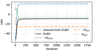
Figure 5: Learning the artificial sparse bars dataset. While the entropy-based ELBO is monotonously increasing, different entropy terms may undergo complex dynamics during the optimization.

For this experiment, we used full covariance Gaussian variational posterior. We observed good convergence and complete recovery of the bars in approximately $70\%$ of runs (7 out of 10). When the model converged to a local optimum, some of the recovered generative fields usually contained two bars, and the final ELBO was slightly lower. During the optimization ELBO values quickly approach the value computed with ground truth $\tilde{W}$, then ELBO values asymptotically converge. Fig. 5 illustrates the typical trajectories of the $\mathcal{L}^{\mathcal{H}}$ and different entropies during the optimization.

E.3 Amortized learning

Our entropy-based objective can be combined with amortized inference and stochastic updates. We used a deep neural network that comprises two ResNet-like nonlinear mappings (parametric automorphisms) and separate linear readout maps for the mean and the diagonal covariance variational parameters of the posterior (Fig. 6), optimized by stochastic updates (Adam with $lr=10^{-3}$). We compared the convergence speed to the previously suggested (non-amortized) EM-like updates, and considered cases with and without prior entropy annealing (Fig. 3). The EM updates with annealing allow the ELBO to be optimized faster and reach a better optimum. We also observe a minor gap (presumably an amortization gap) due to the limited neural network capacity. All three optimization methods finally result in a set of similar generative fields (Fig. 8).

Low-rank approximation of full covariance matrices for the variational posterior (Fig. 7) helps to diminish the amortization gap. To construct a low-rank convariance matrix, the DNN produces a set of $r$ vectors $V\in\mathbb{R}^{H\times r}$, and a separate vecor of diagonal covariances $\sigma^{2}$. The covariance matrix is then computed as $\mathcal{T}=VV^{\mathrm{T}}+\operatorname{diag}(\sigma^{2})$. We used $r=5$ in our experiments.

Figure 6: Deep encoder architecture. First, the input data $\mathbf{x}$ is linearly projected to a higher dimensional space, and then two ResNet-like transformations are applied. The variational parameters $\boldsymbol{\nu}$ and $\sigma^{2}$ are obtained by separate linear mappings. Posterior diagonal covariance is then constructed as $\mathcal{T}=\operatorname{diag}(\sigma^{2})$.

Figure 7: Encoder architecture for variational posterior with a low-rank approximation of full covariance. The covariance matrix is constructed as $\mathcal{T}=VV^{\mathrm{T}}+\operatorname{diag}(\sigma^{2})$.

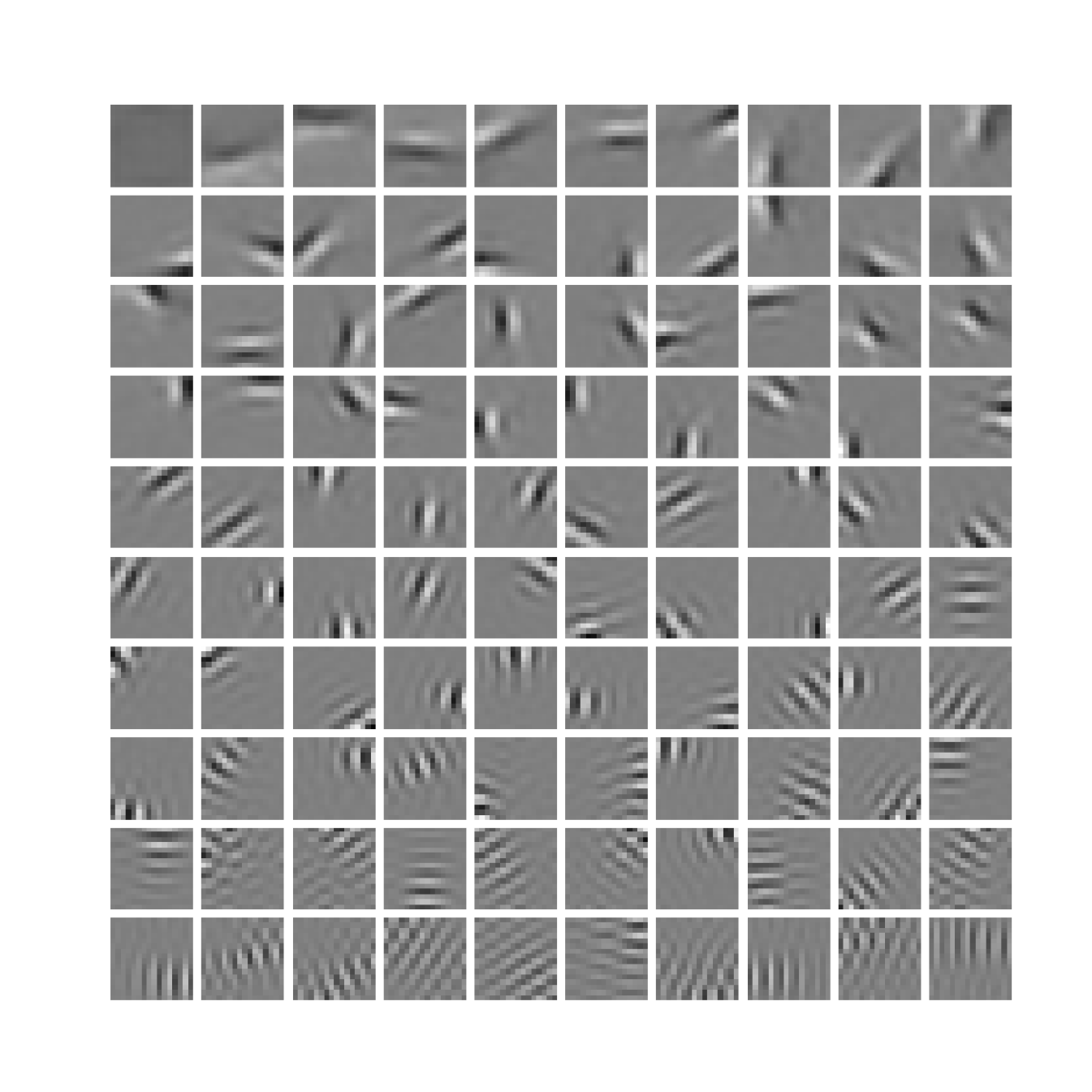
(a) EM, annealing

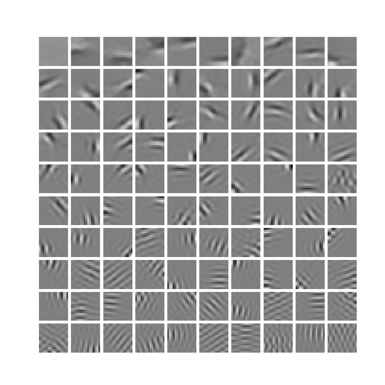
(b) EM, no annealing

(c) Adam, amortized

Figure 8: Learned bases with different optimization methods where the generative fields were obtained after 200 epochs of optimization. All methods result in practically the same set of filters, but the prior entropy annealing facilitates fast convergence.

E.4 Comparing annealing schemes

We used a basic linear annealing scheme for prior entropy annealing: $\gamma_{i}=\max(1.0,2*(5-i))$ for epoch $i$. For the likelihood entropy annealing, we set $\delta_{i}=\min(1.0,1/(7-i))$. While prior (Fig. 10) and likelihood (Fig. 11) entropy annealing result in similar generative fields after convergence, the trajectories of the optimization of generative fields and latent codes differ. With prior entropy annealing, all the latent dimensions are used for the encoding from the very beginning of the optimization. In the case of the likelihood annealing, the latent dimensions start contributing gradually to the reconstruction.

Table 1 provides numerical details and gives some insights into how the model parameters behave during the above-mentioned annealing. The table shows ELBOs, Gini coefficients, and contributions of different entropies to the entropy-based ELBO. To compute the ELBO, after every epoch, we evaluated the non-annealed ELBO for the learned parameters and the full dataset. Thus, the highest (and also the only proper) ELBO can be obtained only when a non-annealed objective is used for the optimization. We selected some of the annealing epochs, for which the contribution of the annealing coefficient causes a quantitatively similar balance of the contributing entropies to the annealed ELBO, that is, e.g., for the epochs when $\gamma=2$ and $\delta=0.5$ the corresponding contributing entropies are close. Despite the similarity in the values of the entropies, the learned generative fields are qualitatively very different (Fig. 10 and Fig. 11). Next, we provide an explanation of what causes such a qualitative difference.

Notice that the Gini coefficient of the latent codes is high during the annealing, which indicates high sparsity of the posterior. Here we have to remember that the likelihood annealing trades off the reconstruction quality to Kullback-Leibler divergence between the prior and the variational posterior. With small $\delta$ we can largely ignore the reconstruction term and focus only on the Kullback-Leibler divergence. Our reparameterized model allows two ways to minimize the Kullback-Leibler divergence term: by adjusting the variational posterior parameters, and by changing the prior scales. We observe both phenomena in the case of the likelihood entropy annealing, which leads to noisy and non-localized generative fields and posterior collapse of some of the latent dimensions. That is, some of the latent dimensions do not participate in the encoding, their corresponding scale parameters $\lambda_{h}$ shrink to very small values, the corresponding contribution to the Kullback-Leibler divergence may become arbitrarily close to 0, and the corresponding generative fields do not contribute to the data reconstruction. Fig. 11 illustrates such noisy generative fields, which do not contribute to the reconstruction. Noisy and non-localized generative fields entirely disappear as the annealing ends.

Figure 9: Prior entropy annealing on natural image patches dataset. Gini coefficients (mean $\pm$SD bars) of the latent codes (Fig. 4 for example generative fields) stay marginally higher if the prior entropy annealing is used even after the annealing ends after epoch 5. The bottom plot shows the annealing schedule.

The qualitative difference of prior entropy annealing can be seen by comparing the generative fields we obtain during the optimization (Fig. 10). Even after one epoch with high weight on the prior entropy, the generative fields already resemble localized Gabor filters. As the annealing decays, more generative fields that represent high-frequency Gabors emerge. Fig. 9 shows the linear annealing schedule and how the Gini coefficient changes during the prior entropy annealing.

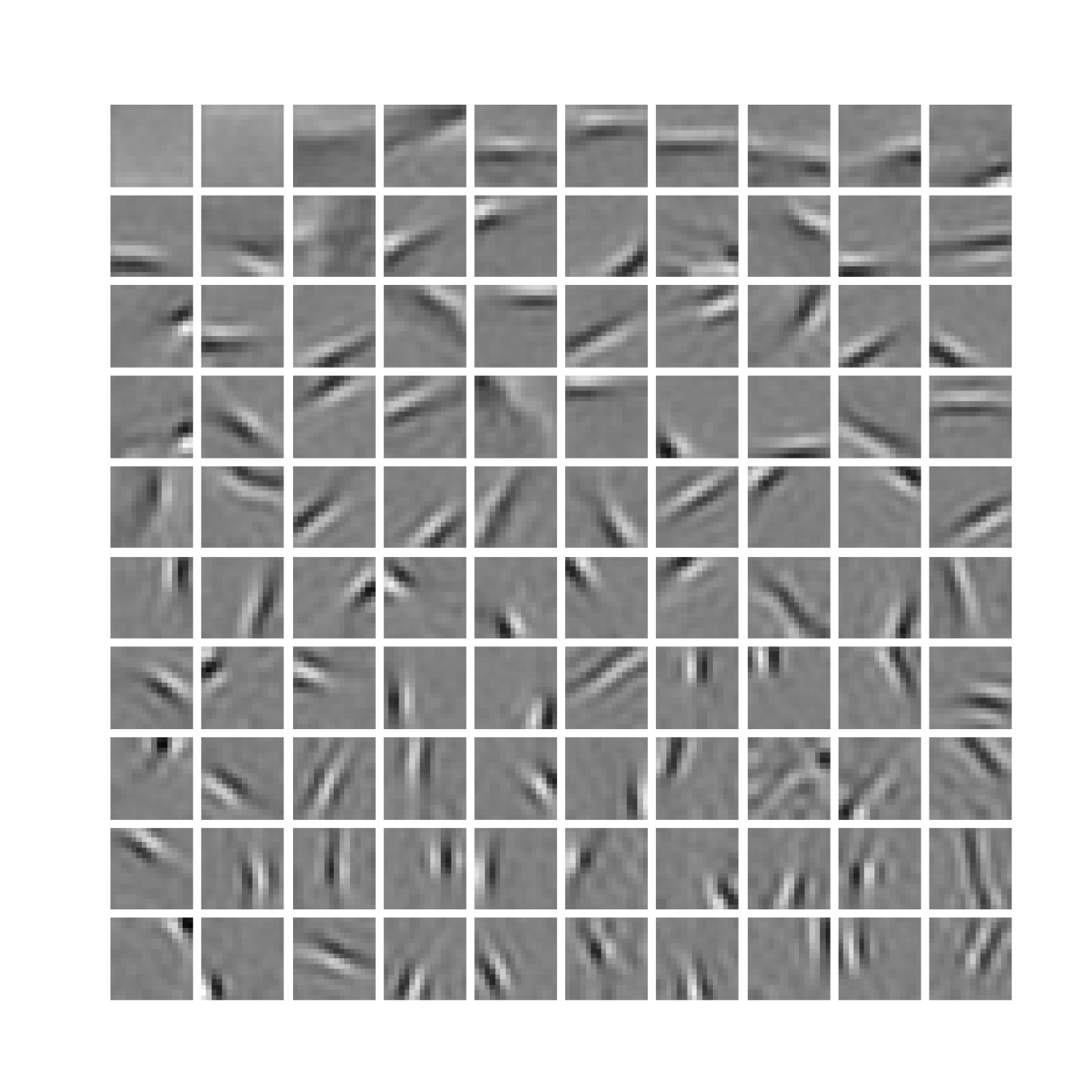
(a) Epoch 1

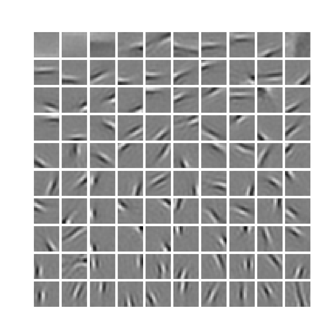
(b) Epoch 2

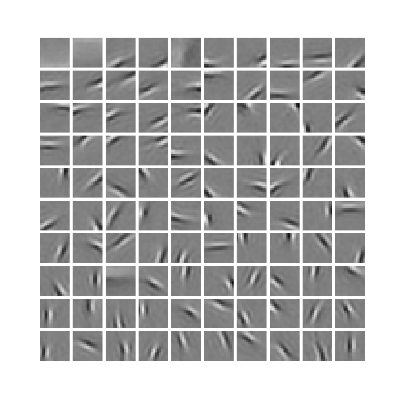
(c) Epoch 3

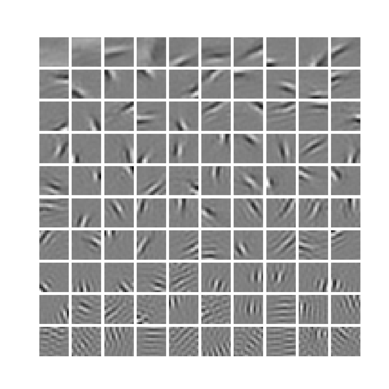
(d) Epoch 4

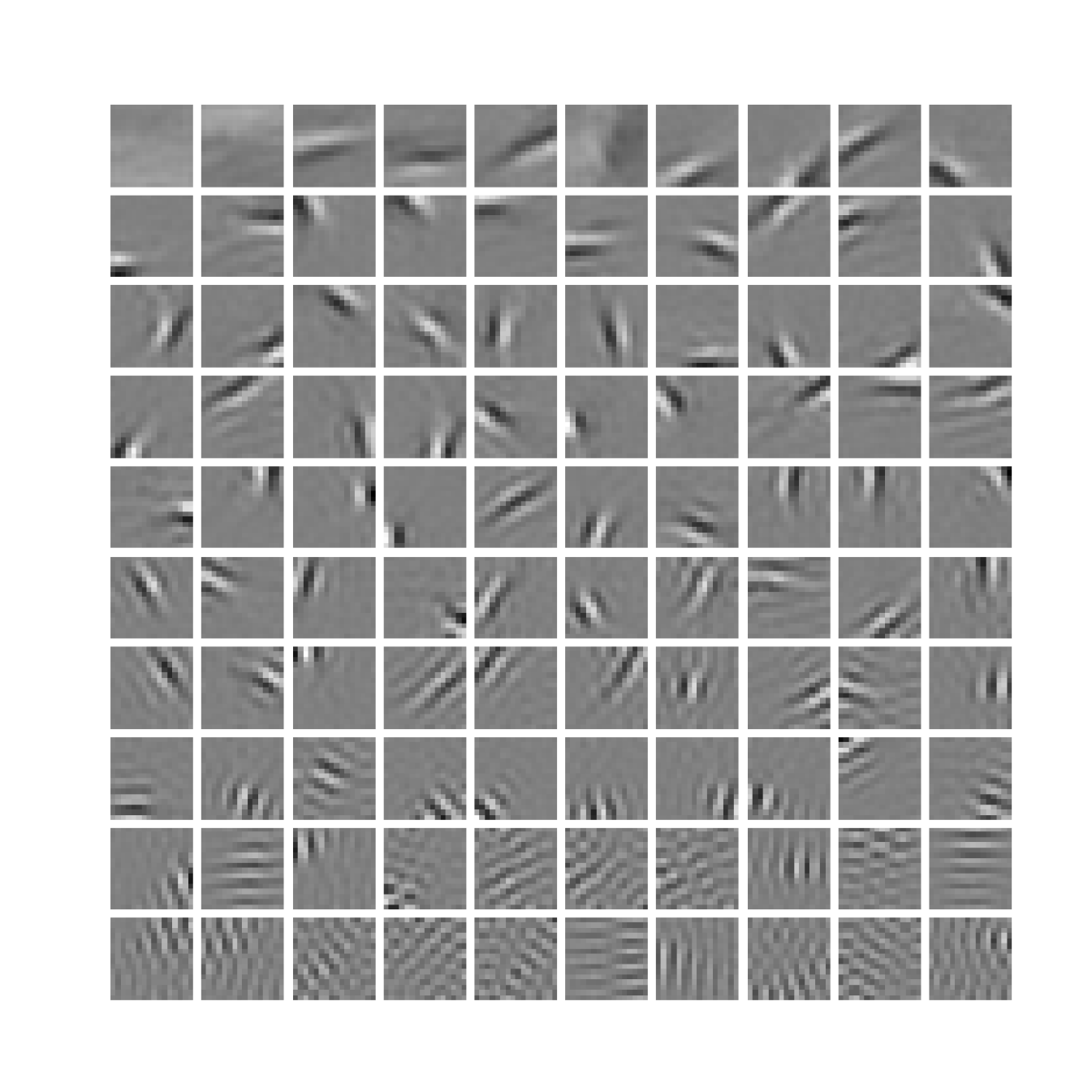
(e) Epoch 5

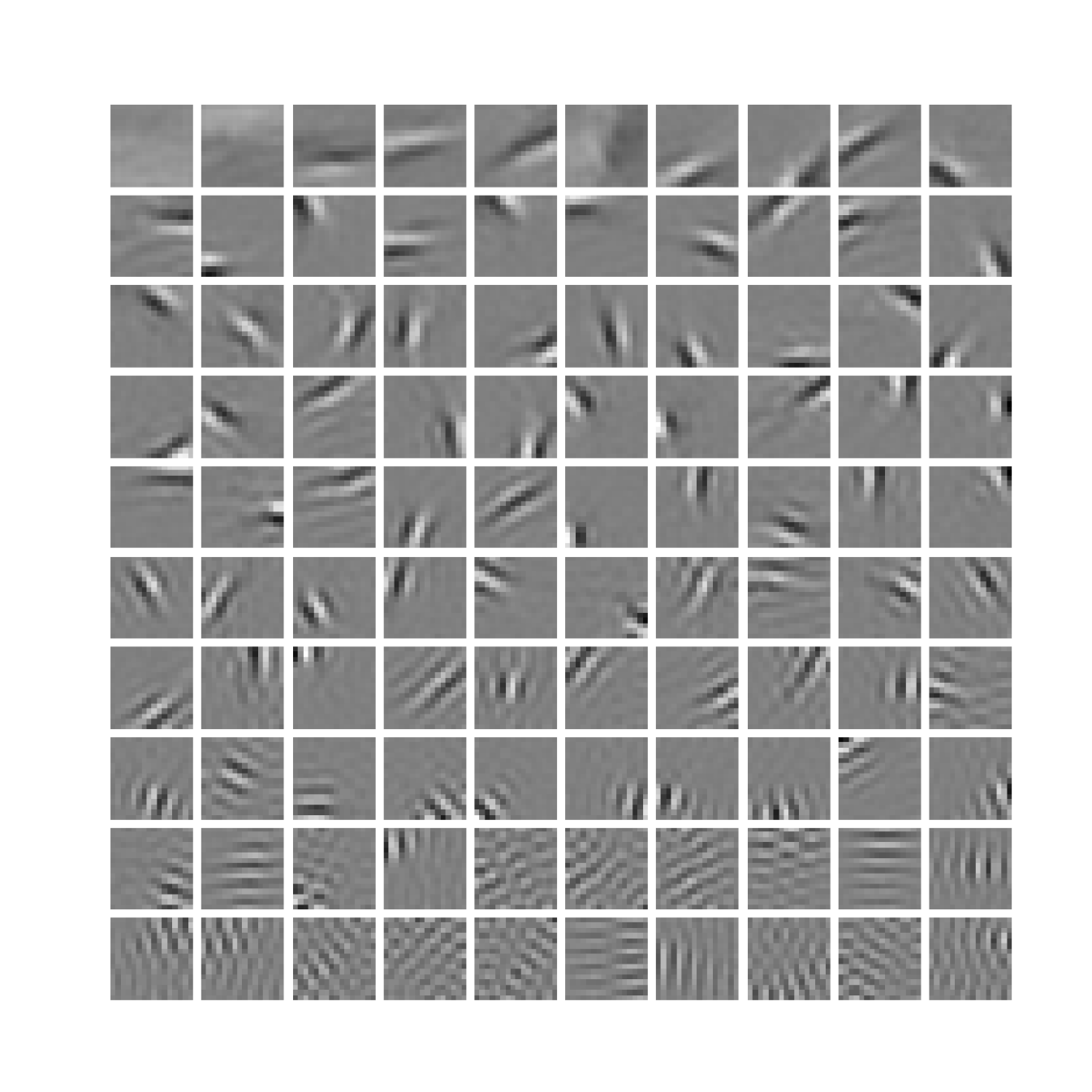
(f) Epoch 6

(g) Epoch 7

(h) Epoch 8

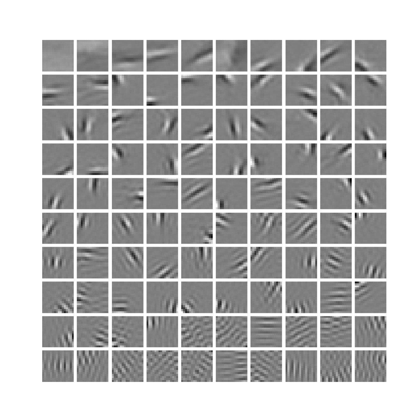
(i) Epoch 9

Figure 10: Learned generative fields during optimization with prior entropy annealing. The annealing stops after epoch 5.

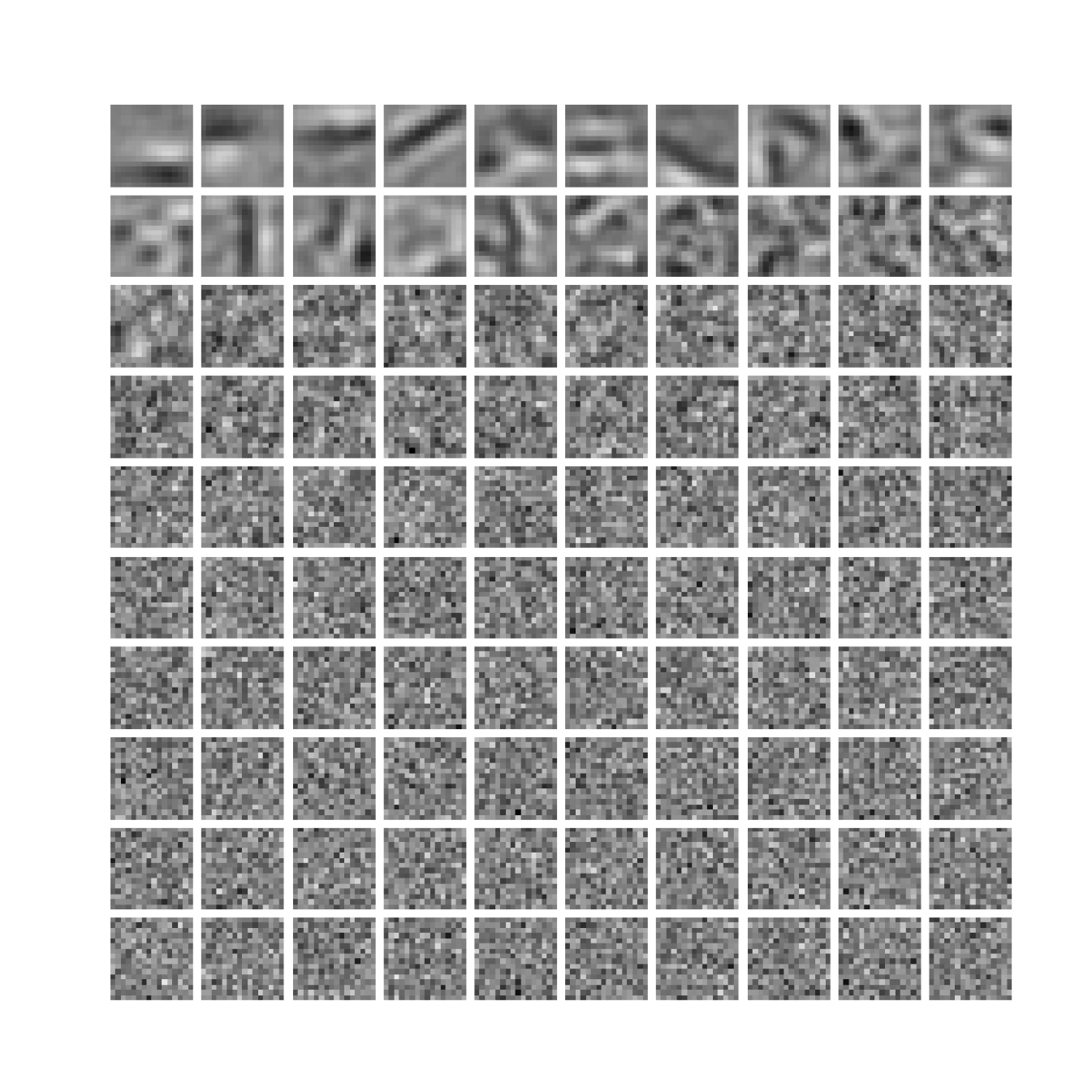
(a) Epoch 1

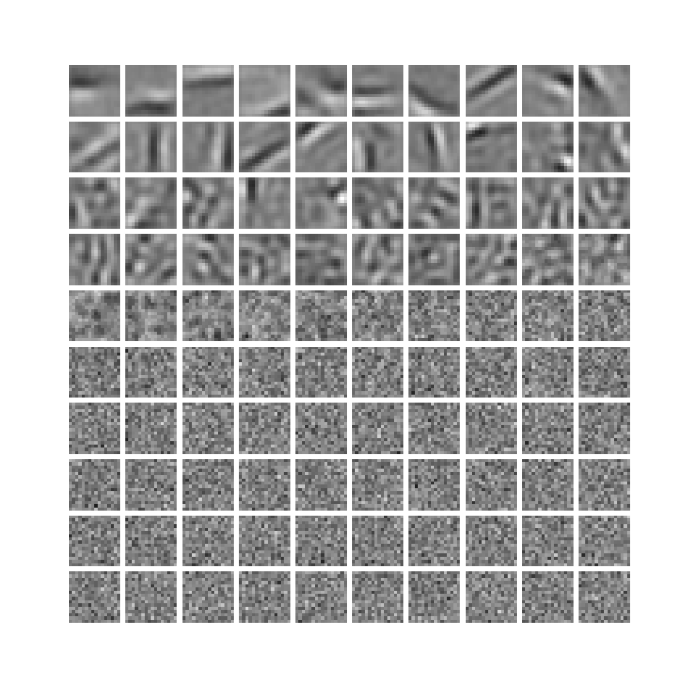
(b) Epoch 2

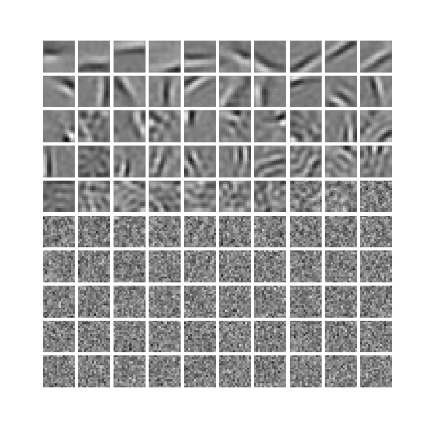
(c) Epoch 3

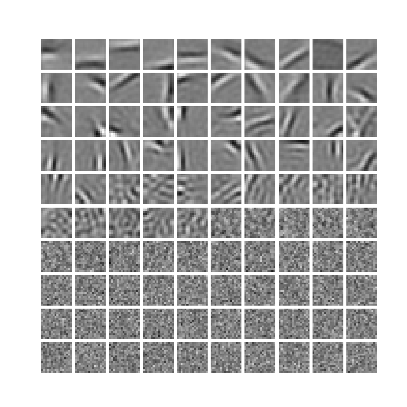
(d) Epoch 4

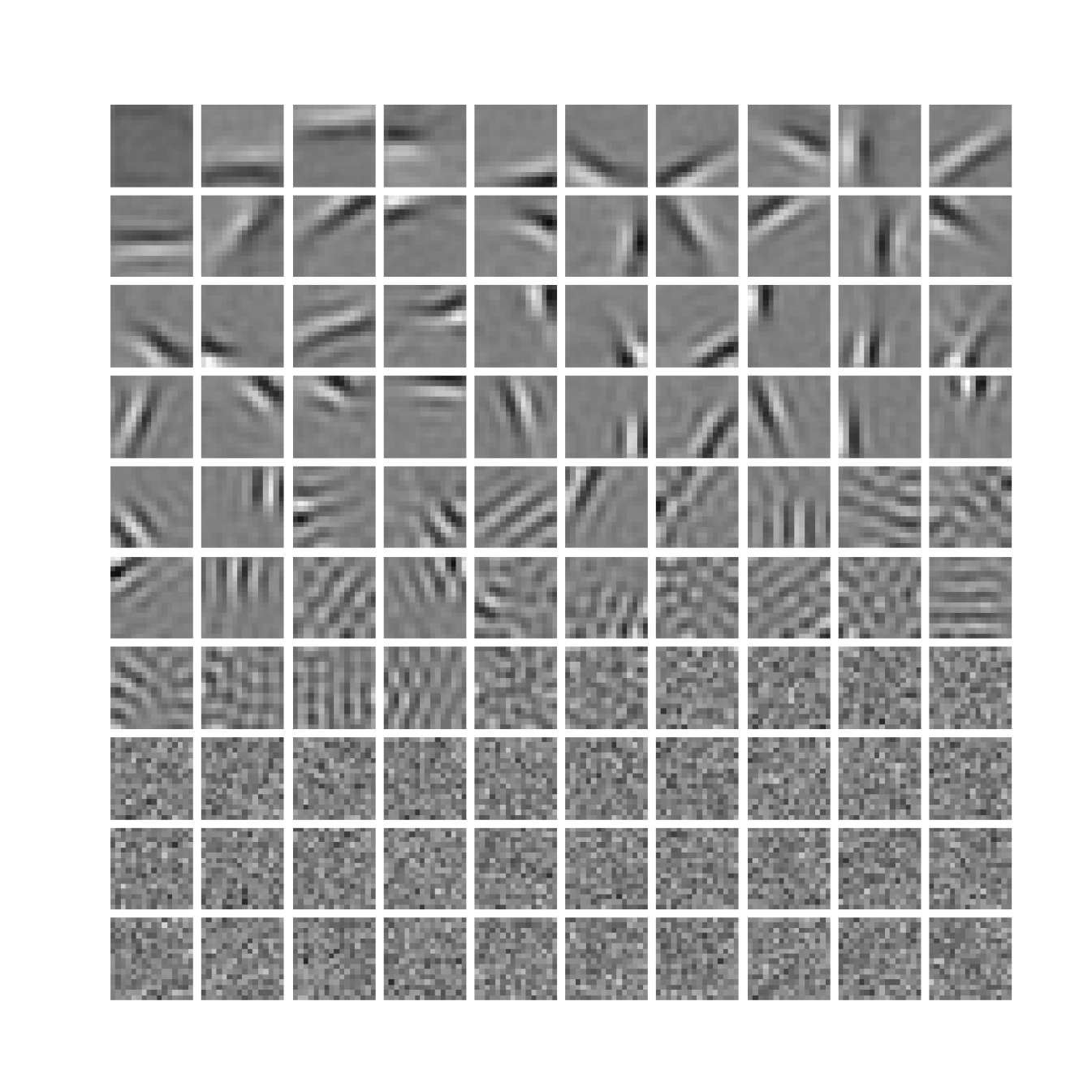
(e) Epoch 5

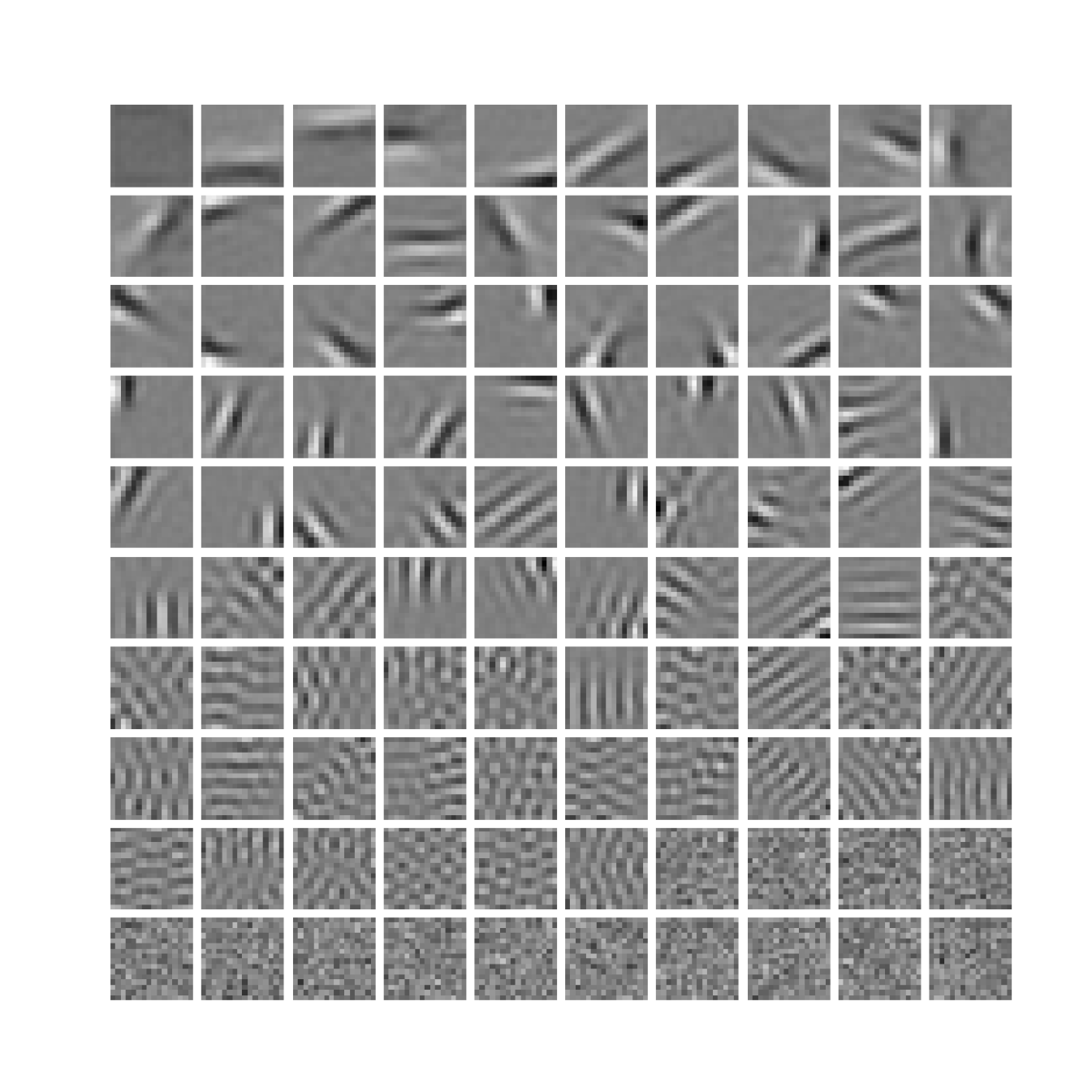
(f) Epoch 6

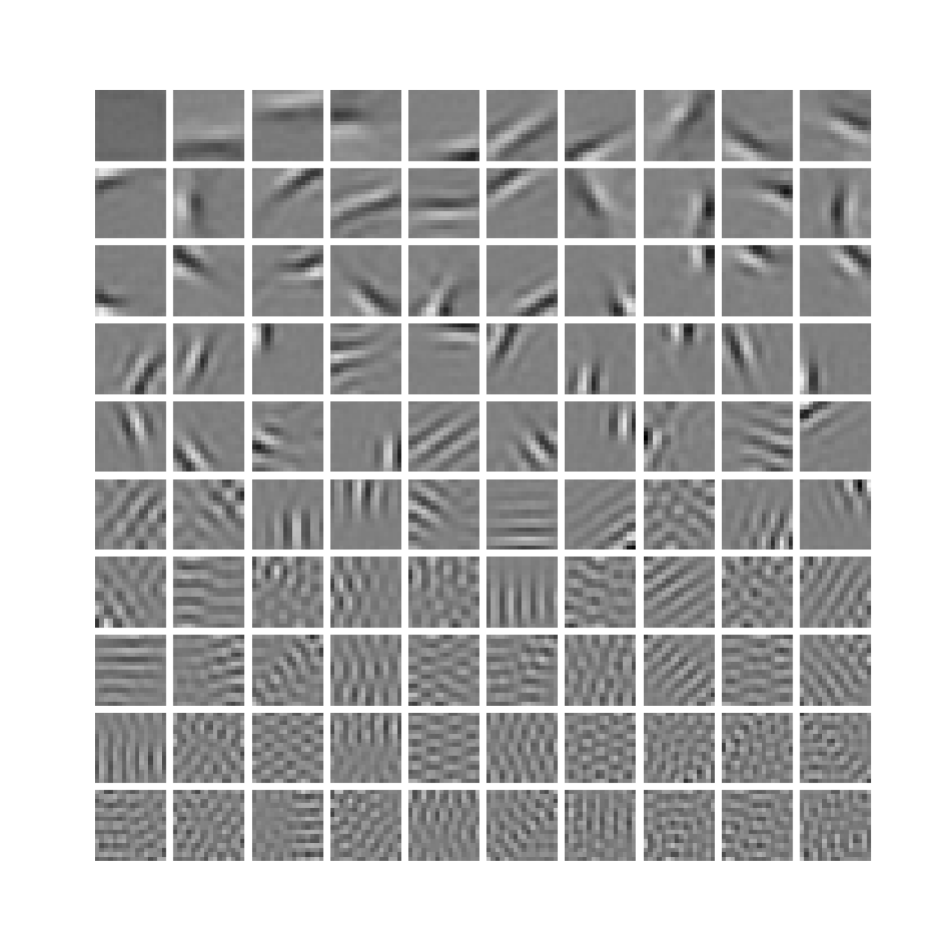
(g) Epoch 7

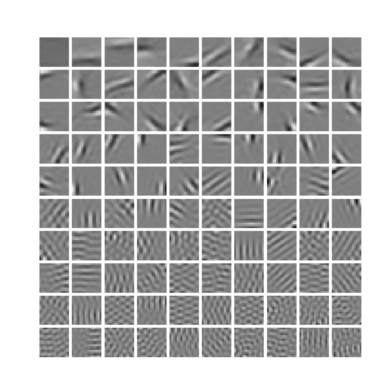
(h) Epoch 8

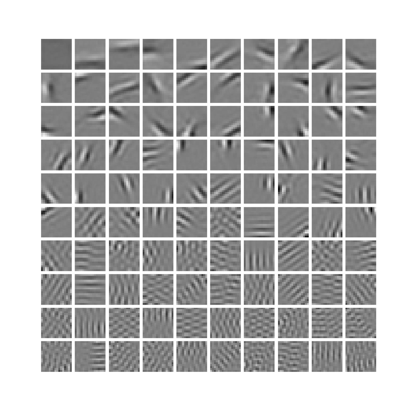
(i) Epoch 9

Figure 11: Learned generative fields during optimization with likelihood annealing of entropy-ELBOs. The annealing stops after epoch 6. It is equivalent to $\beta$-annealing, which is a popular scheme to tune reconstruction–embedding quality trade-off for VAE training.

E.5 Learning overcomplete basis

Prior entropy annealing significantly improves the quality of the learned dictionary and the sparseness of the latent codes (see Fig. 12). When after annealing the prior entropy weight is set to 1, approximately half of the generative fields converge to high-frequency textures and contribute only marginally to the reconstruction. Emphasizing the prior allows us to learn a rich dictionary of localized Gabor-like generative fields that span a wide range of frequencies, positions, and orientations, positively contributing to the sparsity of the latent codes.

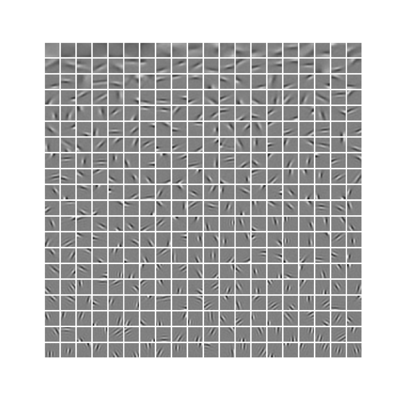
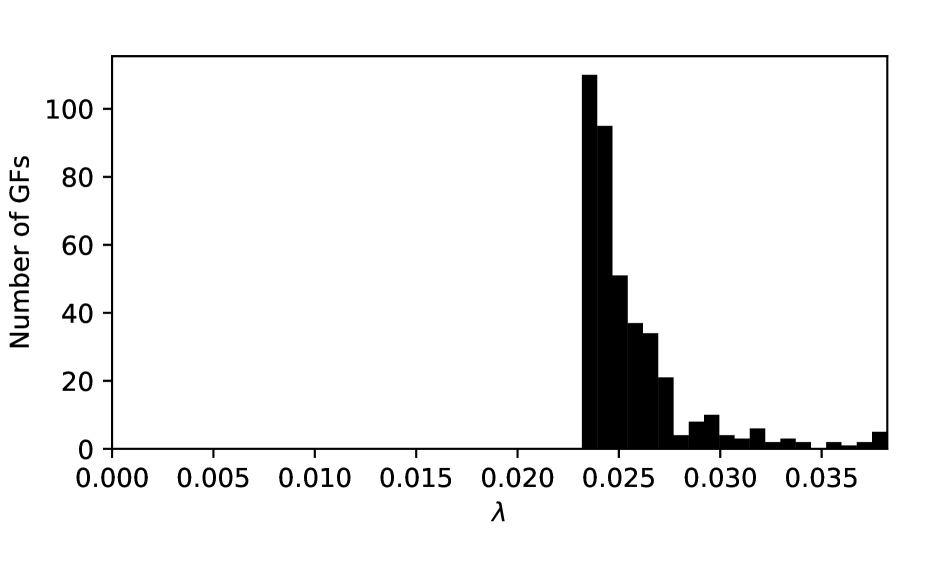
(a) Prior entropy weight: 2

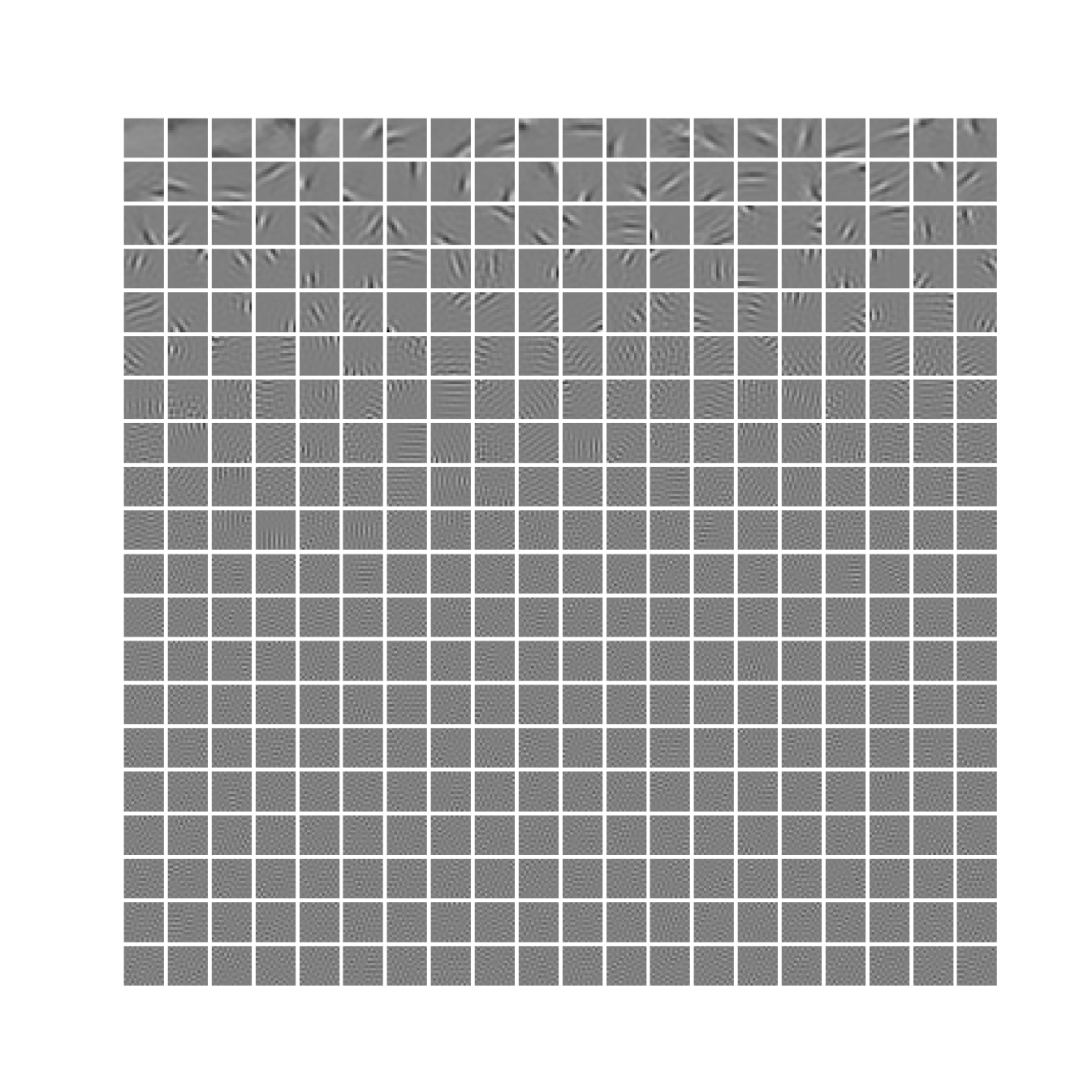
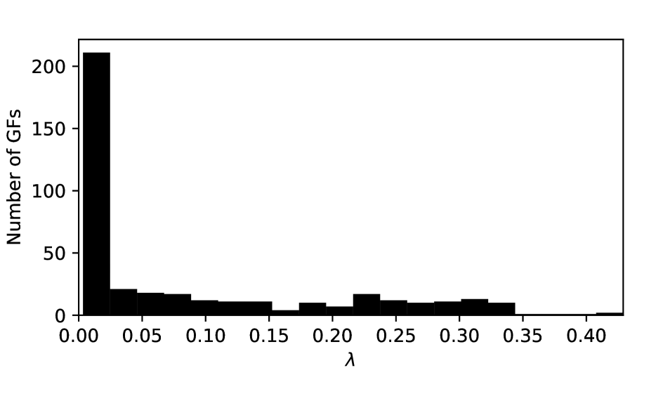
(b) Prior entropy weight: 1

Figure 12: Learned overcomplete bases for the image patches dataset. 400 generative fields are learned from $16\times 16$ image patches. Different generative fields were obtained with prior entropy weight set to 2 (a), and with the original ELBO (b). The bottom histograms illustrate how this reweighting affects the prior scales $\lambda_{i}$. In (b) more than 200 prior coefficients are close to 0, which hints to the posterior collapse. The generative fields are sorted according to their $\lambda_{i}$ scale.

References

• Barber and Bishop (1998) D. Barber and C. M. Bishop. Ensemble learning in bayesian neural networks. Nato ASI Series F Computer and Systems Sciences, 168:215–238, 1998.
• Barello et al. (2018) G. Barello, A. S. Charles, and J. W. Pillow. Sparse-Coding Variational Auto-Encoders. bioRxiv preprint, 2018. doi: 10.1101/399246.
• Beck and Teboulle (2009) A. Beck and M. Teboulle. A Fast Iterative Shrinkage-Thresholding Algorithm for Linear Inverse Problems. SIAM Journal on Imaging Sciences, 2(1):183–202, 2009.
• Berkes et al. (2007) P. Berkes, R. Turner, and M. Sahani. On Sparsity and Overcompleteness in Image Models. In Advances in Neural Information Processing Systems, 2007.
• Challis and Barber (2013) E. Challis and D. Barber. Gaussian Kullback-Leibler approximate inference. Journal of Machine Learning Research, 14(8), 2013.
• Chen et al. (2023) J. Chen, R. Wang, J. He, and M. J. Li. Encouraging Sparsity in Neural Topic Modeling with Non-Mean-Field Inference. In Machine Learning and Knowledge Discovery in Databases: Research Track, pages 142–158, 2023.
• Cheng et al. (2022) L. Cheng, F. Yin, S. Theodoridis, S. Chatzis, and T.-H. Chang. Rethinking Bayesian Learning for Data Analysis: The art of prior and inference in sparsity-aware modeling. IEEE Signal Processing Magazine, 39(6):18–52, 2022.
• Damm et al. (2023) S. Damm, D. Forster, D. Velychko, Z. Dai, A. Fischer, and J. Lücke. The ELBO of Variational Autoencoders Converges to a Sum of Entropies. In Proc. AISTATS, volume 206, pages 3931–3960. PMLR, 2023.
• Daubechies et al. (2004) I. Daubechies, M. Defrise, and C. De Mol. An iterative thresholding algorithm for linear inverse problems with a sparsity constraint. Communications on Pure and Applied Mathematics, 57(11):1413–1457, 2004.
• Drefs et al. (2023) J. Drefs, E. Guiraud, F. Panagiotou, and J. Lücke. Direct Evolutionary Optimization of Variational Autoencoders with Binary Latents. In Proc. ECML 2022, volume 13715 of LNCS/LNAI, pages 357–372. Springer, 2023.
• Fallah and Rozell (2022) K. Fallah and C. J. Rozell. Variational Sparse Coding with Learned Thresholding. In Proc. ICML, pages 6034–6058. PMLR, 2022.
• Földiák (1990) P. Földiák. Forming sparse representations by local anti-Hebbian learning. Biological Cybernetics, 64(2):165–170, 1990.
• Gregor and LeCun (2010) K. Gregor and Y. LeCun. Learning fast approximations of sparse coding. In Proc. ICML, page 399–406, 2010.
• Hastie et al. (2015) T. Hastie, R. Tibshirani, and M. Wainwright. Statistical Learning with Sparsity: The Lasso and Generalizations. CRC press, 2015.
• Higgins et al. (2017) I. Higgins, L. Matthey, A. Pal, C. Burgess, X. Glorot, M. Botvinick, S. Mohamed, and A. Lerchner. beta-vae: Learning basic visual concepts with a constrained variational framework. In Proc. ICLR, 2017.
• Hoyer (2002) P. Hoyer. Non-negative sparse coding. In Proceedings of the 12th IEEE workshop on neural networks for signal processing, pages 557–565. IEEE, 2002.
• Huang et al. (2018) C.-W. Huang, S. Tan, A. Lacoste, and A. C. Courville. Improving Explorability in Variational Inference with Annealed Variational Objectives. In Advances in Neural Information Processing Systems, 2018.
• Hurley and Rickard (2009) N. Hurley and S. Rickard. Comparing Measures of Sparsity. IEEE Transactions on Information Theory, 55(10):4723–4741, 2009.
• Jaakkola and Jordan (1997) T. S. Jaakkola and M. I. Jordan. A Variational Approach to Bayesian Logistic Regression Models and their Extensions. In Sixth International Workshop on Artificial Intelligence and Statistics, pages 283–294. PMLR, 1997.
• Jordan et al. (1999) M. I. Jordan, Z. Ghahramani, T. S. Jaakkola, and L. K. Saul. An Introduction to Variational Vethods for Graphical Models. Machine learning, 37:183–233, 1999.
• Katahira et al. (2008) K. Katahira, K. Watanabe, and M. Okada. Deterministic annealing variant of variational Bayes method. Journal of Physics: Conference Series, 95(1):012015, 2008.
• Kingma and Welling (2014) D. P. Kingma and M. Welling. Auto-encoding variational bayes. In ICLR, 2014.
• Korotkov and Korotkov (2020) N. Korotkov and A. Korotkov. Integrals Related to the Error Function. CRC Press, 2020.
• Korotkov (2002) N. E. Korotkov. Integrals for applications of integral of probabilities. 2002. ISBN 5-900777-10-3. (in Russian).
• Korotkov and Korotkov (2012) N. E. Korotkov and A. N. Korotkov. Integrals Related to the Integrals of Probability. 2012. ISBN 078-5-900777-18-4. (in Russian).
• Kuss and Rasmussen (2005) M. Kuss and C. Rasmussen. Assessing approximations for gaussian process classification. Advances in Neural Information Processing Systems, 18, 2005.
• Lee et al. (2006) H. Lee, A. Battle, R. Raina, and A. Ng. Efficient sparse coding algorithms. In Advances in Neural Information Processing Systems, 2006.
• Liu and Nocedal (1989) D. C. Liu and J. Nocedal. On the limited memory BFGS method for large scale optimization. Mathematical Programming, 45(1):503–528, 1989.
• Lücke (2023) J. Lücke. On the Convergence of the ELBO to Entropy Sums. arXiv preprint arXiv:2209.03077, 2023.
• Lücke and Henniges (2012) J. Lücke and M. Henniges. Closed-form entropy limits – a tool to monitor likelihood optimization of probabilistic generative models. In Proc. AISTATS, pages 731–740. PMLR, 2012.
• Mairal et al. (2014) J. Mairal, F. Bach, and J. Ponce. Sparse Modeling for Image and Vision Processing. Foundations and Trends in Computer Graphics and Vision, 2014.
• Mohamed et al. (2012) S. Mohamed, K. A. Heller, and Z. Ghahramani. Bayesian and L1 approaches for sparse unsupervised learning. In Proc. ICML, pages 683–690, 2012.
• Neal and Hinton (1998) R. M. Neal and G. E. Hinton. A view of the EM algorithm that justifies incremental, sparse, and other variants. In Learning in graphical models, pages 355–368. Springer, 1998.
• Nielsen and Nock (2010) F. Nielsen and R. Nock. Entropies and cross-entropies of exponential families. In 2010 IEEE International Conference on Image Processing, pages 3621–3624, Hong Kong, 2010.
• Olshausen (1996) B. A. Olshausen. Sparse coding simulation software, 1996. URL https://www.rctn.org/bruno/sparsenet/.
• Olshausen and Field (1996) B. A. Olshausen and D. J. Field. Emergence of simple-cell receptive field properties by learning a sparse code for natural images. Nature, 381(6583):607–609, 1996.
• Paszke et al. (2017) A. Paszke, S. Gross, S. Chintala, G. Chanan, E. Yang, Z. DeVito, Z. Lin, A. Desmaison, L. Antiga, and A. Lerer. Automatic differentiation in pytorch. In Neural Information Processing Systems Workshop on Autodiff, 2017.
• Rozell et al. (2008) C. J. Rozell, D. H. Johnson, R. G. Baraniuk, and B. A. Olshausen. Sparse Coding via Thresholding and Local Competition in Neural Circuits. Neural Computation, 20(10):2526–2563, 2008.
• Schöpf and Supancic (2014) H. Schöpf and P. Supancic. On Bürmann’s Theorem and Its Application to Problems of Linear and Nonlinear Heat Transfer and Diffusion. The Mathematica Journal, 16, 2014.
• Seeger et al. (2007) M. Seeger, F. Steinke, and K. Tsuda. Bayesian Inference and Optimal Design in the Sparse Linear Model. In Proc. AISTATS, pages 444–451. PMLR, 2007.
• Seeger (2008) M. W. Seeger. Bayesian Inference and Optimal Design for the Sparse Linear Model. Journal of Machine Learning Research, 9(26):759–813, 2008.
• Sheikh et al. (2014) A.-S. Sheikh, J. A. Shelton, and J. Lücke. A Truncated EM Approach for Spike-and-Slab Sparse Coding. Journal of Machine Learning Research, 15(77):2653–2687, 2014.
• Tipping and Bishop (1999) M. E. Tipping and C. M. Bishop. Probabilistic principal component analysis. Journal of the Royal Statistical Society: Series B (Statistical Methodology), 61(3):611–622, 1999.
• Tonolini et al. (2020) F. Tonolini, B. S. Jensen, and R. Murray-Smith. Variational Sparse Coding. In Proceedings of The 35th Uncertainty in Artificial Intelligence Conference, pages 690–700. PMLR, 2020.
• Williams (1995) P. M. Williams. Bayesian Regularization and Pruning Using a Laplace Prior. Neural Computation, 7(1):117–143, 1995.
• Wipf (2023) D. Wipf. Marginalization is not marginal: No bad vae local minima when learning optimal sparse representations. In Proc. ICML, 2023.
• Yao et al. (2022) D. Yao, S. McLaughlin, and Y. Altmann. Patch-based image restoration using expectation propagation. SIAM Journal on Imaging Sciences, 15(1):192–227, 2022.