The metallicity variations along the chromosome maps: The Globular Cluster 47 Tucanae

Abstract

The ”chromosome maps” (ChMs) of globular clusters (GCs) have revealed that these ancient structures are not homogeneous in metallicity in various ways, and in different natures. The Type II GCs, generally display larger variations, sometimes coupled with slow neutron capture ($s$) element enrichment on the ChMs redder sequences, which has been interpreted as due to multiple generations of stars. On the other hand, most GCs have inhomogeneous first populations (1P) in the form of large ranges in the $\Delta_{\tiny{\mathrm{F275W,F814W}}}$ values, pointing towards a not fully mixed pristine molecular cloud. We analyse the chemical composition the GC 47 Tucanae, which shows both inhomogeneous 1P stars and, although not formally a Type II GC, hosts a small number of stars distributed on a red side of the main stream of ChM stars. Our results suggest that 1P stars are not homogeneous in the overall metallicity, with variations of the order of $\sim$0.10 dex in all the chemical species. The anomalous stars distributed on a redder sequence of the ChM, are further enriched in metals, but without any evidence for a significant enrichment in the $s$ elements. Our three second population stars located on the normal component of the map, have metallicities similar to those of the metal-richer 1P group, suggesting that this population formed from these stars. Although three stars is a too-small sample to draw strong conclusions, the low spread in metals of these objects might point towards a formation in a fully mixed medium, possibly after a cooling flow phase.

1 Introduction

The existence of multiple stellar populations in virtually all globular clusters (GCs) of the Milky Way is a well-established fact (see Gratton et al., 2012; Bastian & Lardo, 2015; Milone & Marino, 2022, for reviews). Yet, the mechanisms responsible for this phenomenon continue to be debated (e.g. Renzini et al., 2015).

The most effective tool to isolate the different populations of stars hosted in a GC is offered by a combination of four bands from the Hubble Space Telescope ($HST$), namely F275W, F336W, F438W and F814W, allowing the construction of multiple pseudo-color plots now known as “Chromosome Maps” (ChMs, Milone et al., 2015). In these diagrams the position of stars is especially sensitive to the abundance of C, N and O elements via the molecules that they form as well as to the helium and iron abundance (e.g. Marino et al., 2008; Milone et al., 2017; Marino et al., 2019a). The ChMs have revolutionized the traditional picture of GCs, and have revealed unexpected features of the multiple population pattern.

On the basis of the ChM shape, GCs have been subdivided into two main groups, namely Type I and Type II. The majority ($\sim$83%) of Milky Way GCs belongs to the Type I class, with the ChM displaying a first population (1P) and different numbers of second population (2P) groups, but following a single “sequence” along the map. ChMs of Type II clusters are more complex. In addition to the common 1P and 2P stars, a second sequence (hereafter anomalous) appears on the red side of their maps (Milone et al., 2017). A large number of spectroscopic studies have demonstrated that stars on the anomalous sequence are metal richer than the normal ones and, in most cases, they also are enriched in the elements produced by the slow neutron capture reactions ($s$ elements) (e.g. Yong & Grundahl, 2008; Marino et al., 2009, 2015, 2021; Johnson et al., 2017; McKenzie et al., 2022).

Perhaps the most shocking discovery from the ChMs was the apparent chemical inhomogeneity of even the 1P, with elemental ratios similar to that of halo field stars. Indeed, in most GCs, the 1P stars themselves do not look as a chemically homogeneous group as they show a large spread in the $m_{\rm F275W}-m_{\rm F814W}$ color, the $x$ axis of the ChMs. This was first noticed by Milone et al. (2015) who hinted at a variation of helium among 1P stars to account for the spread. However, none of the several plausible physical mechanisms considered by Milone et al. (2018) was able to account for an helium enrichment without a concomitant conversion of C and O into N. Thus, either a totally new, unknown process was at work producing a spread in helium among 1P stars, or helium was not the culprit and some other element was driving it.

To shed light on the apparent chemical inhomogeneity of 1P stars, once associated to one single stellar population (the primordial one), spectroscopic tagging in GCs with more pronounced spreads along the 1P on the ChM has promptly followed the photometric findings. The first spectroscopic evidence of metallicity variations among 1P stars has been shown in the GC NGC 3201 ([Fe/H]=$-$1.59 dex), where a small spread of the order of $\sim$0.10 dex has been detected, at constant [O/Fe] and [Na/Fe] (Marino et al., 2019b). These findings suggest indeed that the overall metallicity, rather than helium, is the main factor for the 1P spread along the ChM. Later on, photometric support for internal variations in metallicity among the 1P stars has been reported for several analysed GCs (see Legnardi et al., 2022).

The possibility that 1P stars themselves have an internal spread in the overall metallicity suggests that either the molecular cloud out of which 1P stars formed was not chemically homogeneous, i.e., was not fully mixed following its original chemical enrichment, or while 1P stars were forming some Type Ia supernova from previous generations may have polluted the intra-cluster medium. These options can provide us with new hints to understand the process of GC formation, its time-scale, and help to identify the class of stars responsible for the further enrichment of the interstellar medium (ISM) to form the 2P stars in GCs. In this context, it is noteworthy that hydrodynamical simulations have predicted that metal abundance spreads within GC forming giant molecular clouds can influence the iron abundances of future cluster members (McKenzie & Bekki, 2021).

It is clear now that the chemical enrichment in metallicity, though small, might be a quite common property of Milky Way GCs. The phenomenon seems to be linked to different mechanisms, depending on whether the GC is Type I, and metallicity variations could account for the 1P spread in the $m_{\rm F275W}-m_{\rm F814W}$ color along the ChMs, or Type II where the enrichment of the redder anomalous component could be larger, sometimes associated with further enhancements in the [$s$/Fe] and C+N+O abundances (e.g. Marino et al., 2011a; Yong et al., 2015). In this context, we note that, when spectra of excellent quality are used, very small variations in metals, of the order of a few hundredths of dex are found in both globular and open clusters (e.g. Yong et al., 2013; Liu et al., 2016; Monty et al., 2023; Lardo et al., 2023).

In this work we analyse the chemical pattern of 1P stars in the relatively metal rich GC NGC 104 (47 Tucanae, [Fe/H]=$-$0.72 dex) (Harris, 2010). This bright cluster offers the opportunity to analyse the different metal-enrichment events that these systems can experience. Indeed, 47 Tucanae, besides displaying a well-elongated 1P, shows a very broad ChM sequence of 1P and 2P stars, rather than a clearly split ChM as in Type II clusters. Its broad ChM suggests that it can include metal enriched stars like the anomalous stars in Type II clusters. Thus, 47 Tucanae has not been formally classified as a Type II GC by Milone et al. (2017), but represents an ideal target for an in-depth investigation of both the chemical abundance pattern within 1P stars and other metal enrichment channels associated with its candidate anomalous stars which can the progeny of a faint sub giant branch populated by about 10% of the stars (Anderson et al., 2009).

The layout of this paper is as follows: Section 2 presents the photometric and spectroscopic data; Section 3 describes how we derive atmospheric parameters and the chemical abundance analysis; Section 4 presents our results, that are discussed and summarised in Sections 5-6.

Table 1: Coordinates, Photometric Information (including the location on the ChM), Radial Velocities, with associated rms from the # (number) exposures and maximum time between observations (Time interval) for our 29 spectroscopic targets observed with UVES. The anomalous candidate stars have been highlighted in the last column.

ID	RA	DEC	$V$	$\Delta_{\tiny{\mathrm{F275W,F814W}}}$	$\Delta_{\tiny{C~{}\mathrm{F275W,F336W,F438W}}}$	RV	rmsRV	#	Time interval	anomalous
	[J2000]	[J2000]	[mag]	[mag]	[mag]	[km s-1]	[km s-1]		[months]
8672	00:24:20.5	$-$72:06:00.19	14.97	$-$0.2192	$+$0.0446	$-$13.99	0.93	9	14	no
116624	00:23:52.9	$-$72:04:18.59	13.81	$-$0.1252	$+$0.3932	$-$17.56	0.27	9	14	yes
11746	00:24:15.6	$-$72:06:04.31	14.06	$-$0.0514	$+$0.0653	$+$3.58	0.29	9	14	no
44780	00:24:16.1	$-$72:05:32.89	13.64	$-$0.1588	$+$0.0013	$-$36.37	0.26	9	14	no
68444	00:23:58.0	$-$72:05:03.00	14.90	$-$0.1876	$+$0.0951	$-$12.37	0.35	9	14	no
71504	00:23:54.8	$-$72:05:32.58	14.54	$-$0.0861	$+$0.0603	$-$27.26	0.27	9	14	no
92267	00:24:12.6	$-$72:04:23.67	13.43	$-$0.3425	$+$0.3754	$-$13.04	0.27	11	14	no
115804	00:23:53.6	$-$72:04:48.31	14.00	$-$0.1349	$+$0.0846	$-$28.39	0.08	2	2	no
22386	00:24:02.7	$-$72:05:46.67	14.00	$+$0.0107	$+$0.2369	$-$19.00	0.06	2	2	yes
28653	00:23:54.6	$-$72:05:46.67	14.53	$-$0.0891	$+$0.0871	$-$16.39	0.25	10	5	no
41968	00:24:19.0	$-$72:05:13.88	14.33	$-$0.0929	$+$0.1460	$-$27.99	0.10	2	2	no
61006	00:24:03.6	$-$72:05:06.60	14.52	$-$0.1427	$+$0.0568	$-$19.85	0.10	2	2	no
73063	00:23:53.2	$-$72:05:25.31	14.44	$-$0.2656	$+$0.4352	$-$5.87	0.06	2	2	yes
84553	00:24:21.0	$-$72:04:49.08	14.45	$-$0.1813	$+$0.1326	$-$33.42	0.13	2	2	no
10619	00:24:17.1	$-$72:06:10.60	13.47	$-$0.0842	$-$0.0339	$+$1.33	0.22	9	13	no
112499	00:23:57.2	$-$72:04:17.30	14.13	$-$0.2180	$+$0.0792	$+$10.52	0.28	9	13	no
143175	00:23:59.8	$-$72:03:53.10	14.58	$-$0.1573	$+$0.0434	$-$31.93	0.28	9	13	no
22746	00:24:01.9	$-$72:06:05.41	13.46	$+$0.0110	$-$0.0008	$-$22.62	0.21	9	13	no
70896	00:23:55.5	$-$72:05:00.48	13.77	$-$0.0069	$+$0.0662	$-$1.59	6.72	9	13	no
83377	00:24:22.9	$-$72:04:31.58	14.44	$-$0.0451	$-$0.0195	$-$26.26	0.21	9	13	no
86528	00:24:18.5	$-$72:04:16.09	14.82	$-$0.0041	$+$0.0420	$+$4.21	0.31	9	13	no
90842	00:24:14.0	$-$72:04:14.20	14.53	$+$0.0042	$+$0.0076	$+$4.39	0.25	5	13	no
146316	00:23:55.4	$-$72:04:00.79	14.67	$-$0.1399	$+$0.0973	$-$24.38	0.24	3	5	no
15613	00:24:10.4	$-$72:05:58.37	13.81	$-$0.1329	$+$0.0712	$-$9.06	0.34	8	5	no
69465	00:23:56.8	$-$72:05:09.60	13.88	$-$0.1467	$+$0.1009	$+$12.42	0.29	8	5	no
86281	00:24:18.9	$-$72:04:35.89	13.64	$-$0.0327	$+$0.0670	$+$4.75	0.24	8	5	no
91298	00:24:13.5	$-$72:04:31.50	14.36	$-$0.2290	$+$0.3097	$-$19.00	0.33	8	5	no
9946	00:24:18.2	$-$72:06:03.79	14.80	$-$0.0361	$-$0.0199	$-$14.92	0.24	8	5	no
100719	00:24:06.2	$-$72:04:48.78	13.69	$-$0.2126	$+$0.0517	$-$17.87	0.23	7	12	no

2 Data

2.1 The chromosome map of 47 Tucanae

Milone et al. (2017) analysed the ChMs of 57 GCs, including 47 Tucanae, whose ChM is shown in Figure 1. As noticed by Milone et al. (2017), clearly, the ChM of this cluster covers a large range along the $\Delta_{\tiny{\mathrm{F275W,F814W}}}$ axis, which is not consistent with the 1P stars being chemically homogeneous.

In this work we analyse high-resolution spectra for the targets shown in Figure 1, and couple our spectroscopic data (see Section 2.2) with high-precision photometry from the $HST$. The photometric data come from the $HST$ UV Legacy Survey that is designed to investigate multiple stellar populations in GCs (GO-13297, Piotto et al., 2015). Details on the images and on the data reduction can be found in Piotto et al. (2015) and Milone et al. (2017). Our photometry has been corrected for differential reddening effects as in Milone et al. (2012a, b).

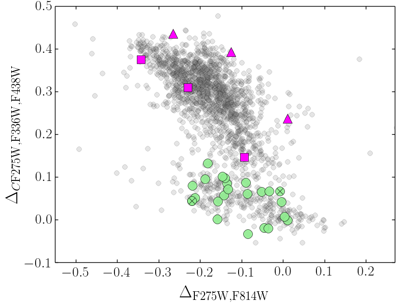
Figure 1: The chromosome map of 47 Tucanae from Milone et al. (2017). Grey dots represent the complete sample of RGB stars used to construct the map. Our spectroscopic targets observed with UVES are highlighted with large coloured symbols. Specifically, green circles are 1P stars, magenta squares are normal 2P stars, while magenta triangles represent candidate anomalous stars. The locations of two RV binaries are indicated by black crosses.

2.2 The spectroscopic dataset

Our spectroscopic data have been acquired using the FLAMES Ultraviolet and Visual Echelle Spectrograph (FLAMES-UVES, Pasquini et al., 2000) on the European Southern Observatory’s (ESO) Very Large Telescope (VLT), through the programme 105.20NB. The observations were taken in the standard RED580 setup, which has a wavelength coverage 4726-6835 Å and a resolution of $R\sim$47,000 (Dekker et al., 2000). Each target has been selected to pass the isolation criteria, namely no neighbors brighter than 1.5 mag within two fiber radii.

The stars were chosen to span a range in $\Delta_{\tiny{\mathrm{F275W,F814W}}}$ as large as possible, and a quite narrow range in $\Delta_{\tiny{C~{}\mathrm{F275W,F336W,F438W}}}$. Indeed, our primary goal was to observe red giants associated to the 1P on the ChM. As shown in Figure 1, most of our targets lie on the 1P, spanning a range of $\sim$0.20 in $\Delta_{\tiny{\mathrm{F275W,F814W}}}$. Because of the limited sample of isolated targets located within the inner $\sim$3′$\times$3′ field, where the ChM has been constructed, not all the UVES fibers could be fed with 1P stars avoiding fiber collisions. Hence, we had the opportunity to observe a few targets on the 2P as well, namely three stars on the blue and three other stars on the red edge of the ChM as indicated in Figure 1. The red targets might be associated with stars that have an enhanced heavy element composition in Type II GCs (e.g. Milone et al., 2017; Marino et al., 2019a, 2021).

Spectra are based on a number of multiple 2775s exposures, which varies from a minimum of 2 to a maximum of 11, depending both on the brightness and priority of each target. Individual exposures have been taken a few months apart to allow us to detect variations in radial velocities (RVs), and identify possible binaries in our sample. Data were reduced using the FLAMES-UVES pipelines within the EsoReflex interface (Ballester et al., 2000), including bias subtraction, flat-field correction, wavelength calibration, sky subtraction and spectral rectification. As an example, Figure 2 shows two portions of our final spectra.

RVs were derived using the iraf@FXCOR task, which cross-correlates the object spectrum with a template. For the template we used a synthetic spectrum obtained through MOOG (version June 2014, Sneden, 1973), computed with a model stellar atmosphere interpolated from the Castelli & Kurucz (2004) grid, adopting parameters (effective temperature/surface gravity/microturbulence/metallicity) = (T_eff/log g/$\xi_{\rm t}$/[A/H]) = (4500 K/2.0/2.0 km s^-1/$-0.70$ 
dex). Each spectrum was corrected to the restframe system, and observed RVs were then corrected to the heliocentric system. Table 1 lists the observed targets, together with their coordinates, photometric information, RVs, number of exposures and time interval between the observations.

We notice that two stars in our sample, namely #8672 and #70896, have larger root mean square deviations (rms) in their RV values obtained from different exposures (rms_RV), hence we treat these two objects as probable binaries, and highlight their location in the figures with black crosses. However, we warn the reader that we cannot rule out the presence of other binaries with no sizeable differences in the RV values in our sample.

The final mean heliocentric RV for our 47 Tucanae giants, excluding the two binary candidates, is $\langle$RV$\rangle$=$-14.2\pm 2.8$ km s^-1 ($\sigma$=14.1 km s^-1), which lies within $\sim$1 $\sigma$ of the value listed in Baumgardt & Hilker (2018) of $\langle$RV$\rangle$=$-17.2\pm 0.1$ km s^-1$\sigma$=11.50 km s^-1 within an average distance of 18.02 arcsec from the cluster centre).

Finally, the individual exposures for each star have been co-added. The signal-to-noise (S/N) ratio for the combined spectra around $\lambda$6300 Å ranges from S/N$\sim$60 to $\sim$200, depending on the brightness of the star and the number of exposures.

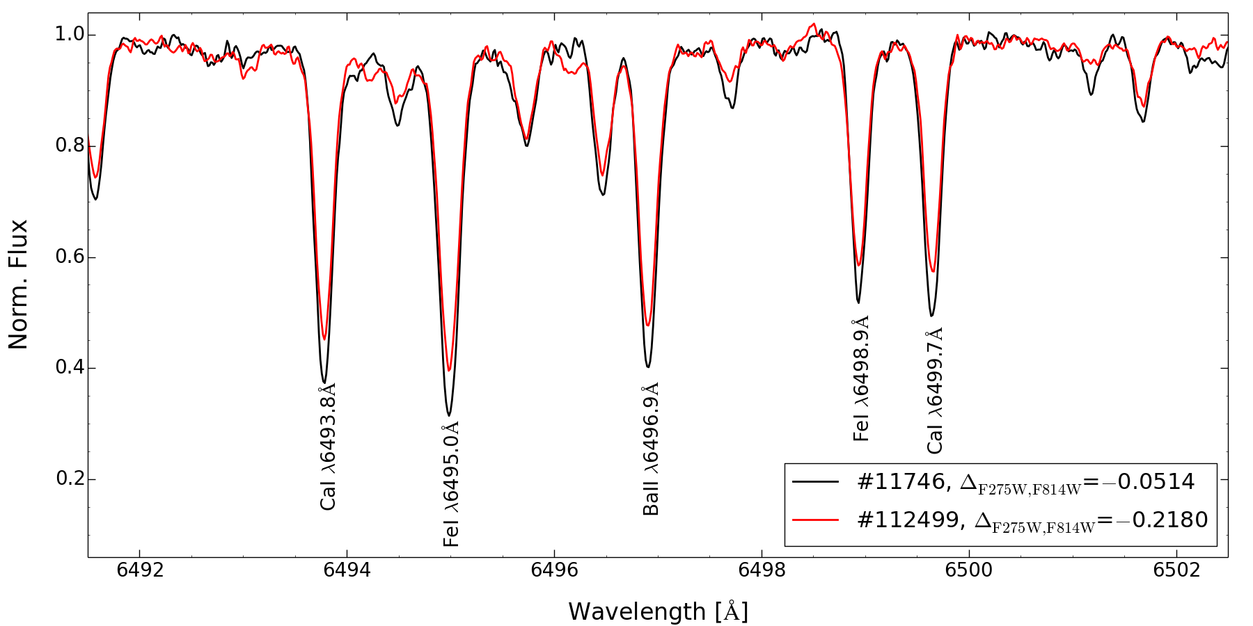
Figure 2: Examples of two portions of FLAMES@UVES spectra including some analyzed Fe and Ca spectral features, plus the Ba line 6496.9 Å. The displayed spectra are relative to stars #11746 and #112499 which have similar atmospheric parameters but different $\Delta_{\tiny{\mathrm{F275W,F814W}}}$ values. Overall, the spectral features of star #11746 (with higher $\Delta_{\tiny{\mathrm{F275W,F814W}}}$) are deeper.

3 Chemical abundance analysis

The UVES spectra have a spectral coverage high enough to allow us a fully-spectroscopical estimate of the stellar parameters, T_eff, log g, [A/H] and $\xi_{\rm t}$. Indeed the number of measured Fe I and Fe II lines for each star is typically 120 and 12, respectively. Briefly, T_eff and log g were inferred by imposing the excitation potential (E.P.) equilibrium of the Fe I lines and the ionization equilibrium between Fe I and Fe II spectral features, respectively. For log g we further imposed Fe II abundances 0.05-0.07 dex higher than the Fe I ones to adjust for non-local thermodynamic equilibrium (non-LTE) effects (Bergemann et al., 2012; Lind et al., 2012). $\xi_{\rm t}$ was set to minimize any dependence of Fe I abundances as a function of equivalent width (EW). The adopted atmospheric parameters are listed in Table 2.

As our sample of stars is composed of giants with information on the ChM obtained from $HST$ filters, our targets are located in the 2.7′$\times$2.7′ innermost region of 47 Tucanae. Hence, we have only star #69465 in common with Carretta et al. (2009a). For this target, our inferred atmospheric parameters are in excellent agreement with those of Carretta and collaborators. Indeed, we obtain differences (Carretta minus this work) of $\Delta\mbox{T${}_{\rm eff}$}=+27$ K, $\Delta\mbox{log~{}{\it g}}=-0.01$, and $\Delta\mbox{$\xi_{\rm t}$}=-0.02$ km s^-1. The larger difference we obtain is in the Fe abundance, $\Delta$[Fe/H]=$+0.13$ dex, which could be likely explained with the different lines used in the two studies, as we exploit UVES data with a larger wavelength coverage and a higher resolution than the GIRAFFE spectra analyzed by Carretta et al. (2009a).

Following our previous work based on data with similar quality, we here adopt typical internal uncertainties in the atmospheric parameters of 50 K for T_eff, 0.20 dex for log g, 0.20 km s^-1 for $\xi_{\rm t}$, and 0.10 dex for metallicity (see Marino et al., 2019b). We also emphasize that systematic errors might be larger.

Table 2: Adopted atmospheric parameters.

ID	Teff	log g	[Fe/H]	$\xi_{\rm t}$
	(K)	(cgs)	dex	(km s-1)
8672	4600	2.20	$-$0.87	1.10
116624	4580	2.20	$-$0.70	1.30
11746	4640	2.30	$-$0.76	1.27
44780	4550	2.15	$-$0.83	1.33
68444	4970	3.05	$-$0.83	0.65
71504	4800	2.70	$-$0.80	0.78
92267	4530	2.07	$-$0.82	1.19
115804	4660	2.33	$-$0.76	1.26
22386	4660	2.35	$-$0.65	1.33
28653	4830	2.75	$-$0.72	1.12
41968	4780	2.60	$-$0.74	1.17
61006	4900	3.00	$-$0.79	0.81
73063	4880	2.80	$-$0.66	1.15
84553	4700	2.30	$-$0.95	1.12
10619	4470	1.95	$-$0.85	1.47
112499	4700	2.47	$-$0.88	0.90
143175	4830	2.80	$-$0.79	1.10
22746	4450	1.97	$-$0.79	1.47
70896	4550	2.15	$-$0.77	1.30
83377	4780	2.60	$-$0.74	1.18
86528	4880	2.90	$-$0.74	0.84
90842	4760	2.60	$-$0.75	0.95
146316	4920	2.95	$-$0.68	0.90
15613	4600	2.20	$-$0.82	1.41
69465	4550	2.12	$-$0.87	1.15
86281	4500	2.10	$-$0.82	1.40
91298	4870	3.02	$-$0.73	1.07
9946	4900	2.85	$-$0.67	1.12
100719	4650	2.30	$-$0.97	0.93

Chemical abundances have been inferred for 22 elements, namely Na, Mg, Al, Si, Ca, Sc (ii), Ti (i and ii), V, Cr (i and ii), Mn, Fe (i and ii), Co, Ni, Cu, Zn, Y (ii), Zr (ii), Ba (ii), La (ii), Pr (ii), Nd (ii), Eu (ii). The abundance analysis has been performed by employing the MOOG code (Sneden, 1973) with the alpha-enhanced Kurucz model atmospheres of Castelli & Kurucz (2004). Chemical abundances have been inferred by using an EW-based analysis; when this was not possible because of blends or hyperfine/isotopic splitting we performed spectral synthesis. We now comment on some of the transitions that we used.

Proton-capture elements: Sodium abundances were determined from the EWs of the Na i doublets at $\sim$5680 Å and $\sim$6150 Å, aluminum from the synthesis of the doublet at $\sim$6667 Å, and magnesium from the EWs of the transitions at $\sim$5528, 5711 Å. Because of the low radial velocity of the cluster, no reliable abundances could be inferred for oxygen, as the [O I] line was masked by much stronger telluric features.

Manganese: Spectral lines around 5399, 5420, 5433, 6014, 6022 Å have been analyzed to infer chemical abundances for Mn. In our synthesis we assume f(${\phantom{}}^{55}$Mn)=1.00 and hyperfine splitting from Lawler et al. (2001a, b) and Kurucz (2009).

Copper: For Cu, we synthesised the spectral feature at $\sim$5105 Å, with both hyperfine and isotopic splitting from Kurucz (2009). Solar-system isotopic fractions of f(${\phantom{}}^{63}$Cu)=0.69 and f(${\phantom{}}^{65}$Cu)=0.31 have been assumed.

Neutron-capture elements: We inferred abundances for Y, Zr, Ba, La, Pr, Nd, and Eu. A spectral synthesis analysis has been employed for Zr ($\lambda$5112 Å), Ba ($\lambda$5854, 6497 Å), La ($\lambda$4921, 5115, 5291, 5302, 5303, 6262, 5936, 6390, 6774 Å), Pr ($\lambda$5323 Å), and Eu ($\lambda$6645 Å), affected by hyperfine and/or isotopic splitting and/or blending features. Barium abundances were computed assuming the McWilliam (1998) $r$-process isotopic composition and hyperfine splitting.

Table 3: Analyzed Chemical Abundances from Na to Sc. Average values for 1P and 2P stars are given for each element at the bottom of the table.

STAR	[Na/Fe]	$\sigma$	#	[Mg/Fe]	$\sigma$	#	[Al/Fe]	$\sigma$	#	[Si/Fe]	$\sigma$	#	[Ca/Fe]	$\sigma$	#	[Sc/Fe]	$\sigma$	#
8672	0.37	0.07	3	0.25	0.00	1	0.43	0.05	2	0.43	0.12	8	0.40	0.27	18	0.13	0.25	3
116624	0.64	0.06	4	0.35	0.00	1	0.47	0.12	2	0.49	0.08	8	0.32	0.20	17	0.22	0.14	6
11746	0.38	0.09	4	0.45	0.00	1	0.21	0.04	2	0.44	0.05	7	0.30	0.15	20	0.24	0.14	6
44780	0.24	0.10	4	0.46	0.00	1	0.21	0.06	2	0.44	0.06	7	0.30	0.17	19	0.23	0.12	6
68444	0.23	0.05	4	0.26	0.00	1	0.06	0.10	2	0.34	0.09	7	0.28	0.14	17	0.18	0.11	6
71504	0.18	0.06	4	0.29	0.00	1	0.15	0.05	2	0.35	0.02	6	0.26	0.13	19	0.23	0.15	6
92267	0.75	0.06	4	0.43	0.00	1	0.32	0.03	2	0.44	0.06	7	0.32	0.19	17	0.27	0.15	6
115804	0.18	0.13	4	0.41	0.00	1	0.16	0.04	2	0.41	0.07	8	0.30	0.16	19	0.20	0.13	6
22386	0.62	0.13	4	0.51	0.00	1	0.28	0.01	2	0.41	0.09	8	0.33	0.17	18	0.23	0.09	6
28653	0.26	0.12	4	0.41	0.00	1	0.12	0.05	2	0.37	0.07	7	0.26	0.13	20	0.24	0.15	6
41968	0.36	0.06	4	0.41	0.00	1	0.15	0.02	2	0.38	0.10	8	0.24	0.13	18	0.22	0.11	6
61006	0.20	0.05	4	0.28	0.00	1	0.07	0.06	2	0.39	0.10	6	0.22	0.12	16	0.26	0.21	5
73063	0.50	0.05	4	0.37	0.00	1	0.23	0.10	2	0.35	0.09	7	0.25	0.17	19	0.30	0.13	6
84553	0.47	0.14	3	0.40	0.00	1	0.21	0.07	2	0.39	0.09	7	0.30	0.09	10	0.12	0.13	6
10619	0.29	0.12	4	0.51	0.00	1	0.24	0.08	2	0.45	0.04	8	0.28	0.16	17	0.22	0.11	6
112499	0.20	0.04	4	0.35	0.00	1	0.10	0.04	2	0.38	0.06	6	0.23	0.12	16	0.26	0.15	6
143175	0.20	0.11	4	0.38	0.00	1	0.11	0.05	2	0.39	0.06	8	0.26	0.15	18	0.28	0.12	6
22746	0.30	0.14	4	0.47	0.00	1	0.20	0.06	2	0.45	0.04	8	0.28	0.17	19	0.22	0.11	6
70896	0.27	0.09	4	0.45	0.00	1	0.14	0.02	2	0.43	0.02	7	0.31	0.15	17	0.22	0.12	6
83377	0.25	0.12	4	0.46	0.00	1	0.16	0.04	2	0.37	0.03	7	0.28	0.14	19	0.22	0.12	6
86528	0.19	0.07	4	0.34	0.00	1	0.18	0.05	2	0.39	0.07	8	0.27	0.19	16	0.28	0.13	6
90842	0.18	0.06	4	0.40	0.00	1	0.12	0.03	2	0.37	0.17	7	0.30	0.17	18	0.28	0.18	5
146316	0.18	0.06	4	0.16	0.20	2	0.06	0.12	2	0.28	0.21	7	0.26	0.15	18	0.30	0.08	5
15613	0.38	0.10	4	0.48	0.00	1	0.18	0.04	2	0.46	0.07	8	0.29	0.15	17	0.22	0.12	6
69465	0.28	0.08	4	0.39	0.00	1	0.14	0.02	2	0.46	0.08	7	0.30	0.16	19	0.24	0.14	6
86281	0.38	0.11	4	0.46	0.00	1	0.18	0.07	2	0.49	0.05	7	0.28	0.16	18	0.26	0.11	6
91298	0.56	0.04	4	0.31	0.00	1	0.19	0.12	2	0.42	0.07	7	0.27	0.15	15	0.31	0.15	6
9946	0.17	0.12	4	0.37	0.00	1	0.14	0.03	2	0.32	0.06	8	0.26	0.12	18	0.25	0.08	6
100719	0.30	0.08	4	0.37	0.00	1	0.15	0.05	2	0.39	0.11	8	0.34	0.17	16	0.15	0.15	6
$<$[X/Fe]$>_{\rm 1P}$	0.26			0.38			0.16			0.40			0.28			0.23
$\pm$	0.02			0.02			0.02			0.01			0.01			0.01
$\sigma$	0.08			0.09			0.08			0.05			0.04			0.04
$<$[X/Fe]$>_{\rm 2P}$	0.57			0.40			0.27			0.41			0.29			0.24
$\pm$	0.06			0.03			0.05			0.02			0.01			0.03
$\sigma$	0.13			0.07			0.11			0.05			0.04			0.06

Table 4: Analyzed Chemical Abundances from Ti to Ni. Average values for 1P and 2P stars are given for each element at the bottom of the table.

STAR	[Ti/Fe]i	$\sigma$	#	[Ti/Fe]ii	$\sigma$	#	[V/Fe]	$\sigma$	#	[Cr/Fe]i	$\sigma$	#	[Cr/Fe]ii	$\sigma$	#	[Mn/Fe]	$\sigma$	#	[Co/Fe]	$\sigma$	#	[Ni/Fe]	$\sigma$	#
8672	0.35	0.23	14	0.30	0.20	3	0.22	0.16	11	$-$0.31	0.07	4	$-$0.15	0.24	2	$-$0.55	0.17	5	$-$0.18	0.06	2	0.13	0.23	24
116624	0.33	0.15	21	0.25	0.06	4	0.34	0.13	12	$-$0.15	0.10	4	$+$0.05	0.01	2	$-$0.26	0.02	5	$+$0.07	0.10	2	0.10	0.16	22
11746	0.33	0.10	23	0.31	0.05	4	0.33	0.21	14	$-$0.10	0.06	4	$+$0.20	0.05	2	$-$0.23	0.04	5	$+$0.08	0.12	2	0.11	0.15	24
44780	0.33	0.14	23	0.38	0.07	6	0.45	0.25	16	$-$0.07	0.06	5	$+$0.10	0.07	2	$-$0.24	0.02	5	$+$0.10	0.14	2	0.11	0.14	27
68444	0.31	0.10	22	0.34	0.07	4	0.25	0.12	13	$-$0.10	0.13	4	$+$0.08	0.07	2	$-$0.31	0.05	5	$-$0.04	0.10	2	0.10	0.13	25
71504	0.31	0.11	22	0.28	0.06	4	0.26	0.14	13	$-$0.06	0.10	4	$+$0.01	0.05	2	$-$0.33	0.04	5	$-$0.01	0.11	2	0.10	0.15	25
92267	0.33	0.14	23	0.29	0.09	4	0.39	0.22	14	$-$0.12	0.10	4	$+$0.05	0.03	2	$-$0.31	0.03	5	$+$0.05	0.17	2	0.11	0.15	24
115804	0.30	0.11	22	0.27	0.03	4	0.30	0.22	13	$-$0.10	0.12	4	$+$0.06	0.01	2	$-$0.32	0.03	5	$+$0.06	0.13	2	0.08	0.14	25
22386	0.35	0.12	21	0.27	0.09	4	0.46	0.21	13	$-$0.06	0.10	4	$+$0.05	0.28	2	$-$0.27	0.04	5	$+$0.12	0.20	2	0.06	0.15	23
28653	0.31	0.14	23	0.31	0.04	4	0.26	0.15	14	$-$0.04	0.10	3	$+$0.09	0.15	2	$-$0.27	0.03	5	$+$0.08	0.06	2	0.11	0.12	23
41968	0.35	0.11	23	0.28	0.08	4	0.31	0.16	13	$-$0.06	0.11	4	$+$0.07	0.02	2	$-$0.29	0.03	5	$+$0.07	0.15	2	0.09	0.14	23
61006	0.30	0.13	20	0.30	0.14	4	0.22	0.14	13	$-$0.07	0.20	4	$+$0.17	0.15	2	$-$0.38	0.08	5	$+$0.15	0.06	2	0.08	0.14	23
73063	0.33	0.12	22	0.34	0.03	4	0.38	0.25	12	$-$0.13	0.19	4	$+$0.14	0.18	2	$-$0.25	0.03	5	$+$0.08	0.07	2	0.13	0.13	23
84553	0.44	0.17	9	0.31	0.04	3	0.61	0.44	5	$+$0.16	0.18	3	–	–	0	$-$0.32	0.10	5	$+$0.16	0.08	2	0.09	0.16	20
10619	0.36	0.10	19	0.29	0.03	3	0.39	0.26	14	$-$0.13	0.06	4	$+$0.12	0.05	2	$-$0.23	0.02	5	$+$0.15	0.13	2	0.10	0.12	25
112499	0.31	0.07	20	0.41	0.19	3	0.26	0.15	13	$-$0.02	0.11	4	$+$0.02	0.02	2	$-$0.35	0.05	5	$-$0.02	0.08	2	0.13	0.17	25
143175	0.29	0.10	23	0.35	0.05	4	0.23	0.14	13	$-$0.11	0.10	4	$+$0.10	0.06	2	$-$0.28	0.04	5	$+$0.03	0.11	2	0.11	0.12	25
22746	0.35	0.13	22	0.30	0.04	4	0.46	0.26	12	$-$0.10	0.08	4	$+$0.13	0.09	2	$-$0.18	0.05	5	$+$0.19	0.21	2	0.11	0.13	25
70896	0.34	0.14	19	0.28	0.09	3	0.40	0.23	13	$-$0.12	0.09	4	$+$0.07	0.08	2	$-$0.34	0.07	5	$+$0.19	0.19	2	0.12	0.14	25
83377	0.31	0.10	23	0.26	0.02	4	0.25	0.14	13	$-$0.04	0.10	4	$+$0.12	0.14	2	$-$0.25	0.03	5	$+$0.05	0.13	2	0.09	0.13	25
86528	0.31	0.12	18	0.34	0.17	2	0.22	0.17	12	$-$0.16	0.15	3	$-$0.06	0.01	2	$-$0.27	0.05	5	$+$0.07	0.07	2	0.14	0.17	24
90842	0.28	0.11	22	0.30	0.06	4	0.24	0.17	12	$-$0.11	0.14	4	$+$0.05	0.02	2	$-$0.31	0.04	5	$+$0.09	0.14	2	0.11	0.18	25
146316	0.29	0.16	23	0.30	0.04	3	0.28	0.17	15	$-$0.10	0.22	4	$+$0.22	0.26	2	$-$0.28	0.05	5	$+$0.15	0.21	2	0.14	0.16	23
15613	0.36	0.09	21	0.33	0.07	4	0.35	0.19	13	$-$0.10	0.08	3	$+$0.10	0.05	2	$-$0.21	0.05	5	$+$0.09	0.10	2	0.10	0.13	24
69465	0.28	0.10	23	0.37	0.08	4	0.27	0.18	13	$-$0.12	0.09	4	$+$0.05	0.07	2	$-$0.30	0.02	5	$+$0.05	0.11	2	0.11	0.15	25
86281	0.35	0.11	20	0.33	0.04	3	0.41	0.25	11	$-$0.09	0.06	4	$+$0.10	0.11	2	$-$0.21	0.03	5	$+$0.14	0.16	2	0.14	0.16	23
91298	0.35	0.12	23	0.35	0.10	4	0.30	0.14	13	$-$0.10	0.08	4	$+$0.16	0.02	2	$-$0.25	0.04	5	$+$0.10	0.10	2	0.14	0.14	24
9946	0.33	0.15	23	0.28	0.06	4	0.27	0.20	13	$+$0.02	0.11	3	$+$0.11	0.08	2	$-$0.25	0.01	5	$+$0.09	0.05	2	0.10	0.13	24
100719	0.32	0.15	22	0.26	0.05	3	0.28	0.12	13	$-$0.10	0.08	4	$-$0.03	0.02	2	$-$0.38	0.09	5	$+$0.01	0.07	2	0.10	0.13	26
$<$[X/Fe]$>_{\rm 1P}$	0.32			0.31			0.30			$-$0.10			0.08			$-$0.29			0.07			0.11
$\pm$	0.01			0.01			0.02			0.01			0.02			0.02			0.02			0.00
$\sigma$	0.02			0.04			0.08			0.06			0.08			0.08			0.08			0.02
$<$[X/Fe]$>_{\rm 2P}$	0.35			0.30			0.40			$-$0.07			0.09			$-$0.28			0.09			0.10
$\pm$	0.02			0.01			0.04			0.04			0.02			0.01			0.02			0.01
$\sigma$	0.04			0.04			0.11			0.11			0.05			0.03			0.04			0.03

Table 5: Analyzed Chemical Abundances from Cu to Eu. Average values for 1P and 2P stars are given for each element at the bottom of the table.

STAR	[Cu/Fe]	[Zn/Fe]	$\sigma$	#	[Y/Fe]	$\sigma$	#	[Zr/Fe]	[Ba/Fe]	$\sigma$	#	[La/Fe]	$\sigma$	#	[Pr/Fe]	[Nd/Fe]	$\sigma$	#	[Eu/Fe]
8672	$-$0.63	$+$0.03	0.00	1	$-$0.14	0.26	2	0.20	$+$0.40	0.04	2	0.17	0.19	7	0.22	0.18	–	1	0.40
116624	$-$0.05	–	–	0	$+$0.15	0.27	3	0.33	$+$0.33	0.05	2	0.16	0.18	9	0.12	0.30	0.15	2	0.46
11746	$-$0.06	$+$0.09	0.00	1	$+$0.09	0.11	3	0.19	$+$0.22	0.13	2	0.19	0.13	9	0.29	0.30	0.16	2	0.50
44780	$-$0.09	$+$0.28	0.01	2	$+$0.06	0.26	3	0.25	$+$0.24	0.05	2	0.21	0.18	9	0.27	0.38	0.15	2	0.54
68444	$-$0.35	$+$0.12	0.00	1	$+$0.04	0.15	3	0.22	$+$0.31	0.01	2	0.29	0.14	7	0.30	0.33	0.20	2	0.62
71504	$-$0.26	$+$0.22	0.00	1	$+$0.06	0.18	3	0.30	$+$0.34	0.02	2	0.33	0.17	8	0.33	0.41	0.16	2	0.56
92267	$-$0.22	$+$0.14	0.00	1	$+$0.05	0.18	3	0.18	$+$0.16	0.03	2	0.17	0.16	9	0.23	0.36	0.13	2	0.44
115804	$-$0.10	–	–	0	$+$0.14	0.24	3	0.20	$+$0.23	0.05	2	0.23	0.12	9	0.15	0.47	–	1	0.48
22386	$+$0.00	$+$0.15	0.00	1	$+$0.16	0.31	3	0.32	$+$0.30	0.08	2	0.34	0.06	8	0.34	0.51	–	1	0.55
28653	$-$0.23	$+$0.20	0.00	1	$+$0.09	0.14	3	0.23	$+$0.32	0.11	2	0.31	0.10	8	0.35	0.42	0.03	2	0.65
41968	$+$0.13	$+$0.25	0.00	1	$+$0.15	0.31	3	0.40	$+$0.15	0.21	2	0.30	0.09	8	0.38	0.53	0.14	2	0.60
61006	$-$0.43	$+$0.24	0.00	1	$+$0.09	0.13	3	0.32	$+$0.24	0.19	2	0.44	0.07	4	0.35	0.53	0.00	2	9999
73063	$-$0.05	$+$0.31	0.00	1	$+$0.19	0.15	3	0.26	$+$0.28	0.13	2	0.27	0.14	6	0.30	0.45	0.05	2	0.50
84553	$-$0.31	$-$0.09	0.00	1	$+$0.40	0.24	3	0.24	$+$0.23	0.54	2	0.41	0.38	5	0.33	0.22	–	1	9999
10619	$-$0.01	$+$0.13	0.00	1	$+$0.04	0.24	3	0.23	$+$0.16	0.02	2	0.19	0.20	9	0.27	0.50	–	1	0.56
112499	$-$0.36	$+$0.23	0.00	1	$+$0.06	0.25	3	0.22	$+$0.30	0.13	2	0.24	0.15	8	0.28	0.35	0.18	2	0.58
143175	$+$0.03	–	–	0	$+$0.17	0.11	3	0.20	$+$0.31	0.18	2	0.30	0.18	8	0.37	0.33	0.18	2	0.59
22746	$+$0.02	–	–	0	$+$0.09	0.23	3	0.21	$+$0.16	0.00	2	0.24	0.18	9	0.26	0.62	–	1	0.53
70896	$-$0.42	$+$0.02	0.00	1	$-$0.09	0.29	2	0.20	$-$0.05	0.05	2	0.16	0.16	9	0.25	0.39	0.17	2	0.54
83377	$-$0.11	$+$0.06	0.00	1	$+$0.04	0.17	3	0.19	$+$0.23	0.10	2	0.24	0.14	9	0.20	0.35	0.20	2	0.65
86528	$-$0.50	$-$0.21	0.00	1	$-$0.04	0.09	3	0.35	$+$0.38	0.10	2	0.31	0.17	7	0.32	0.23	0.02	2	0.68
90842	$-$0.29	$-$0.05	0.00	1	$+$0.05	0.13	3	0.23	$+$0.24	0.16	2	0.22	0.09	9	0.26	0.44	0.18	2	0.63
146316	$-$0.30	$+$0.01	0.00	1	$+$0.10	0.18	3	0.30	$+$0.28	0.28	2	0.35	0.12	6	0.34	0.46	0.12	2	9999
15613	$-$0.04	$+$0.17	0.00	1	$+$0.05	0.18	3	0.20	$+$0.16	0.06	2	0.22	0.20	9	0.29	0.32	0.18	2	0.55
69465	$-$0.42	$+$0.21	0.00	1	$+$0.01	0.21	3	0.19	$+$0.27	0.07	2	0.15	0.14	9	0.15	0.35	0.14	2	0.51
86281	$-$0.21	$+$0.07	0.00	1	$+$0.06	0.33	3	0.21	$+$0.17	0.01	2	0.20	0.16	9	0.28	0.41	0.16	2	0.55
91298	$-$0.20	$+$0.07	0.00	1	$+$0.24	0.11	3	0.30	$+$0.37	0.03	2	0.39	0.10	7	0.42	0.53	0.22	2	0.60
9946	$+$0.00	$+$0.29	0.00	1	$+$0.16	0.14	3	0.17	$+$0.32	0.12	2	0.28	0.11	7	0.30	0.48	–	1	0.62
100719	$-$0.70	$-$0.05	0.00	1	$+$0.01	0.16	3	0.18	$+$0.14	0.07	2	0.23	0.13	9	0.19	0.25	0.08	2	0.59
$<$[X/Fe]$>_{\rm 1P}$	$-$0.25	0.11			0.05			0.23	0.24			0.25			0.27	0.39			0.57
$\pm$	0.05	0.03			0.02			0.01	0.02			0.02			0.01	0.02			0.02
$\sigma$	0.21	0.13			0.07			0.05	0.10			0.07			0.06	0.10			0.07
$<$[X/Fe]$>_{\rm 2P}$	$-$0.10	0.14			0.19			0.29	0.26			0.29			0.30	0.41			0.53
$\pm$	0.06	0.06			0.04			0.03	0.03			0.04			0.04	0.05			0.03
$\sigma$	0.15	0.14			0.11			0.07	0.08			0.10			0.10	0.12			0.07

The inferred chemical abundances are listed in Tables 3-4-5. Internal uncertainties to these abundances introduced by errors in the atmospheric parameters were estimated by varying the stellar parameters, one at a time, by T_eff/log g/[A/H]/$\xi_{\rm t}$=$\pm$50 K/$\pm$0.20 cgs/$\pm$0.10 dex/$\pm$0.20 km s^-1. The contribution due to the limits of our spectra, e.g. the finite S/N that affects the measurements of EWs and the spectral synthesis ($\sigma_{\rm S/N}$), was estimated as the average rms listed in Tables 3-4-5 divided by the square root of the typical number of the analysed spectral features. For those elements with only one line available, a larger error of 0.15 dex has been adopted. Our error budget is listed in Table 6. The total uncertainty $\sigma_{\rm total}$ is the quadratic sum of the errors introduced by the individual contributions.

Table 6: Sensitivity of the derived abundances to the uncertainties in atmospheric parameters and uncertainties due to the limited S/N of our spectra. We reported the total internal uncertainty ($\sigma_{\rm total}$) associated to individual stars obtained by the quadratic sum of all the contributors to the error.

	$\Delta$Teff	$\Delta$log g	$\Delta$$\xi_{\rm t}$	$\Delta$[A/H]	$\Delta$Teff	$\sigma_{\rm S/N}$	$\sigma_{\rm total}$
	$\pm$100 K	$\pm$0.20	$\pm$0.20 km s-1	$\pm$0.10 dex	$\pm$50 K
$\rm{[Na/Fe]}$	$\pm$0.01	$\mp$0.03	$\pm$0.05	$\mp$0.01	$\pm$0.01	$\pm$0.05	$\pm$0.08
$\rm{[Mg/Fe]}$	$\mp$0.01	$\mp$0.03	$\pm$0.01	$\mp$0.01	$\mp$0.00	$\pm$0.15	$\pm$0.15
$\rm{[Al/Fe]}$	$\pm$0.06	$\mp$0.00	$\mp$0.01	$\mp$0.01	$\pm$0.03	$\pm$0.04	$\pm$0.05
$\rm{[Si/Fe]}$	$\mp$0.10	$\pm$0.03	$\pm$0.07	$\pm$0.01	$\mp$0.05	$\pm$0.03	$\pm$0.10
$\rm{[Ca/Fe]}$	$\pm$0.03	$\mp$0.04	$\mp$0.00	$\mp$0.01	$\pm$0.02	$\pm$0.04	$\pm$0.06
$\rm{[Sc/Fe]}$ ii	$\pm$0.07	$\mp$0.01	$\mp$0.00	$\mp$0.01	$\pm$0.04	$\pm$0.06	$\pm$0.07
$\rm{[Ti/Fe]}$ i	$\pm$0.08	$\mp$0.02	$\pm$0.01	$\mp$0.02	$\pm$0.04	$\pm$0.03	$\pm$0.06
$\rm{[Ti/Fe]}$ ii	$\pm$0.05	$\mp$0.02	$\mp$0.01	$\mp$0.01	$\pm$0.03	$\pm$0.04	$\pm$0.06
$\rm{[V/Fe]}$	$\pm$0.09	$\mp$0.01	$\pm$0.00	$\mp$0.02	$\pm$0.05	$\pm$0.06	$\pm$0.08
$\rm{[Cr/Fe]}$ i	$\pm$0.06	$\mp$0.02	$\mp$0.01	$\mp$0.01	$\pm$0.03	$\pm$0.06	$\pm$0.07
$\rm{[Cr/Fe]}$ ii	$\pm$0.02	$\mp$0.01	$\pm$0.02	$\mp$0.01	$\pm$0.01	$\pm$0.06	$\pm$0.07
$\rm{[Mn/Fe]}$	$\pm$0.10	$\pm$0.02	$\mp$0.02	$\mp$0.01	$\pm$0.05	$\pm$0.02	$\pm$0.06
$\rm{[Fe/H]}$ i	$\pm$0.07	$\pm$0.01	$\mp$0.09	$\pm$0.01	$\pm$0.03	$\pm$0.01	$\pm$0.10
$\rm{[Fe/H]}$ ii	$\mp$0.09	$\pm$0.10	$\mp$0.05	$\pm$0.03	$\mp$0.05	$\pm$0.03	$\pm$0.13
$\rm{[Co/Fe]}$	$\mp$0.00	$\pm$0.02	$\pm$0.05	$\pm$0.00	$\pm$0.00	$\pm$0.08	$\pm$0.10
$\rm{[Ni/Fe]}$	$\mp$0.03	$\pm$0.03	$\pm$0.03	$\pm$0.01	$\mp$0.01	$\pm$0.03	$\pm$0.05
$\rm{[Cu/Fe]}$	$\pm$0.11	$\mp$0.00	$\mp$0.09	$\mp$0.03	$\pm$0.07	$\pm$0.15	$\pm$0.19
$\rm{[Zn/Fe]}$	$\mp$0.12	$\pm$0.04	$\mp$0.02	$\pm$0.02	$\mp$0.06	$\pm$0.15	$\pm$0.17
$\rm{[Y/Fe]}$ ii	$\pm$0.08	$\mp$0.02	$\mp$0.04	$\mp$0.01	$\pm$0.04	$\pm$0.14	$\pm$0.15
$\rm{[Zr/Fe]}$ ii	$\pm$0.03	$\pm$0.07	$\mp$0.02	$\pm$0.02	$\pm$0.02	$\pm$0.15	$\pm$0.17
$\rm{[Ba/Fe]}$ ii	$\pm$0.01	$\pm$0.06	$\mp$0.16	$\pm$0.03	$\pm$0.00	$\pm$0.07	$\pm$0.19
$\rm{[La/Fe]}$ ii	$\pm$0.03	$\pm$0.07	$\mp$0.02	$\pm$0.01	$\pm$0.01	$\pm$0.06	$\pm$0.10
$\rm{[Pr/Fe]}$ ii	$\pm$0.00	$\pm$0.08	$\mp$0.01	$\pm$0.03	$\mp$0.00	$\pm$0.15	$\pm$0.17
$\rm{[Nd/Fe]}$ ii	$\pm$0.12	$\mp$0.02	$\mp$0.02	$\mp$0.00	$\pm$0.06	$\pm$0.14	$\pm$0.15
$\rm{[Eu/Fe]}$ ii	$\mp$0.01	$\pm$0.08	$\pm$0.00	$\pm$0.04	$\mp$0.01	$\pm$0.15	$\pm$0.17

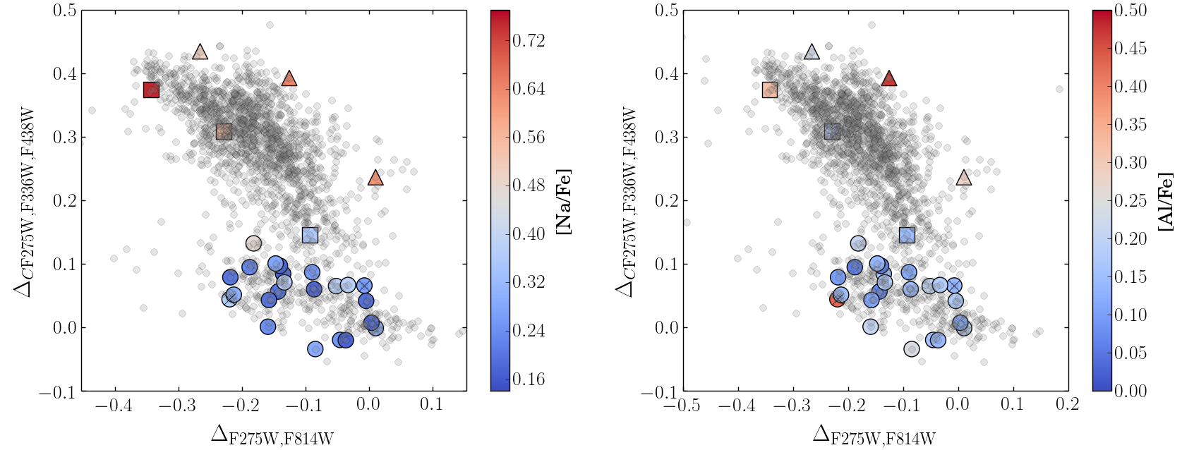
Figure 3: Location of our spectroscopic targets along the ChM of 47 Tucanae from Milone et al. (2017). The color of each star is indicative of the inferred chemical abundances, as illustrated in the color bar. In these two plots we illustrate the chemical pattern of Na and Al abundances relative to Fe.

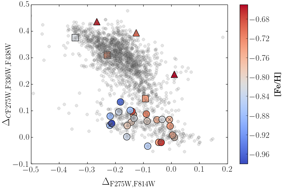
Figure 4: As Figure 3, but for [Fe/H].

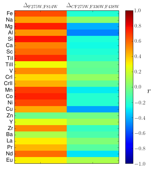
Figure 5: Chemical abundances ${\rm log}\epsilon$(X) as a function of $\Delta_{\tiny{\mathrm{F275W,F814W}}}$ and $\Delta_{\tiny{C~{}\mathrm{F275W,F336W,F438W}}}$ values on the ChM of 47 Tucanae. The color code is indicative of the Spearman correlation coefficient ($r$). The coefficients and their associated significance are listed in Table 7.

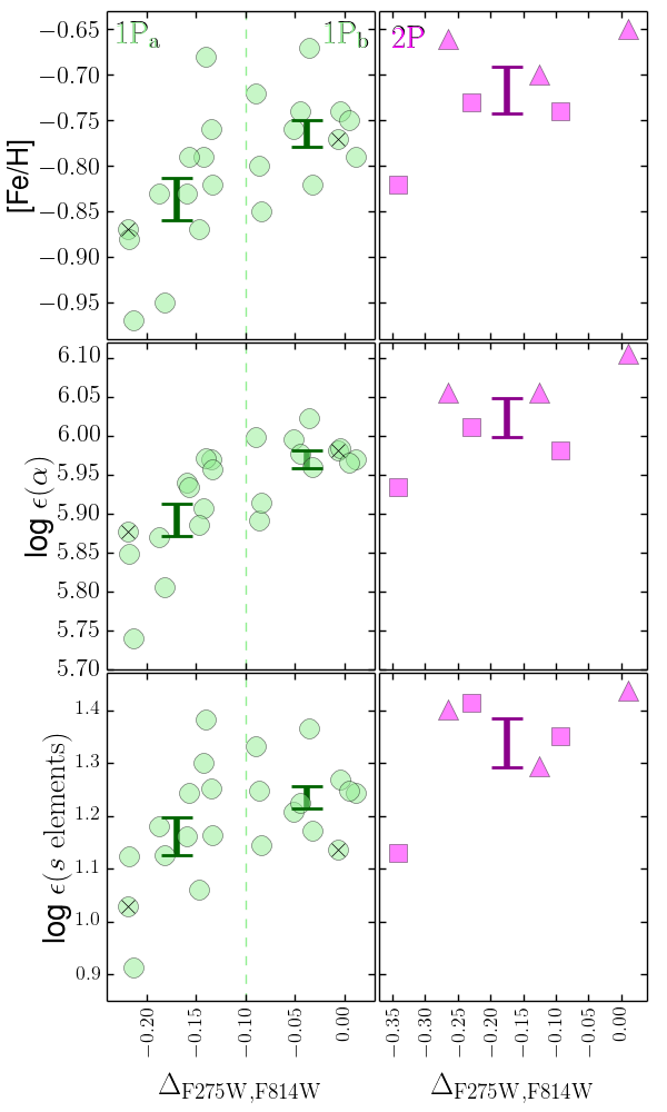
Figure 6: From top to bottom, [Fe/H] and absolute chemical abundances for all the $\alpha$ and the $s$ elements as a function of $\Delta_{\tiny{\mathrm{F275W,F814W}}}$ values on the ChM of 47 Tucanae. Left and right panels represent 1P and 2P stars, respectively. The dashed line on the left panel at $\Delta_{\tiny{\mathrm{F275W,F814W}}}$=$-$0.10 separates the two groups of $\rm{1P_{a}}$ and $\rm{1P_{b}}$ stars (see text for details). The plotted error bars represent the dispersion of the values in each group divided by the square root of the number of stars. Symbols are as in Figure 1.

Table 7: Spearman correlation coefficient ($r$), and associated significance, between chemical abundances log$\epsilon$(X) and the ChM $\Delta_{\tiny{\mathrm{F275W,F814W}}}$ values. Lower % reflects a more important correlation.

Element	$r$	Significance (%)
Fe	0.62	1.0
Na	0.47	1.7
Mg	0.77	0.8
Al	0.48	5.0
Si	0.73	0.0
Ca	0.58	4.8
Sc ii	0.60	0.2
Ti i	0.66	3.4
Ti ii	0.44	6.2
V	0.55	1.2
Cr i	0.43	4.7
Cr ii	0.49	0.3
Mn	0.71	0.1
Co	0.73	0.0
Ni	0.62	0.1
Cu	0.50	1.5
Zn	0.17	26.9
Y ii	0.29	19.0
Zr ii	0.52	17.2
Ba ii	0.15	35.9
La ii	0.31	20.0
Pr ii	0.46	17.1
Nd ii	0.60	0.2
Eu ii	0.62	12.2

4 Chemical abundances along the ChM of 47 Tucanae

Overall, for our 29 stars we obtain a mean iron abundance of [Fe/H]=$-$0.78$\pm$0.02 dex (rms=0.08 dex), consistent with the value of [Fe/H]=$-$0.72 dex listed in Harris (2010). As typical of Population II stars, 47 Tucanae stars are $\alpha$ enhanced in all the analysed $\alpha$ elements, namely Mg, Si, Ca, and Ti.

In this section we analyse the chemical abundance pattern along the ChM of 47 Tucanae. First, we discuss on the 1P/2P chemical differences, and then the abundances internal to the 1P.

4.1 Light elements

As shown in Figure 1, the ChM of 47 Tucanae clearly displays a sharp separation between 1P and 2P stars occurring at $\Delta_{\tiny{C~{}\mathrm{F275W,F336W,F438W}}}$$\sim$0.1. Although our sample was not specifically designed to analyse 2P stars, it includes six giants belonging to this stellar population. From the average chemical abundances listed in Tables 3-4-5, larger differences are observed in the elements involved in the hot-H burning processes, namely Na and Al, as expected for 2P stars in GCs. The six 2P stars are significantly enhanced in sodium by $\Delta$[Na/Fe]_2P-1P=0.31$\pm$0.06 and mildly enhanced in aluminum by $\Delta$[Al/Fe]_2P-1P=0.11$\pm$0.05.

No obvious variations are observed in neither [Mg/Fe] or [Si/Fe], being the observed dispersions similar to those expected from observational errors (see Table 6). Small rms values in these chemical species have been also reported in Carretta et al. (2009b).

For both Na and Al, the observed spread in each population is larger for the 2P stars, consistent with the large range in $\Delta_{\tiny{C~{}\mathrm{F275W,F336W,F438W}}}$ of these stars (see Marino et al., 2019a). Looking at the distribution of Na and Al along the ChM, as displayed in Figure 3, the most Na rich star (#92267) is located on the ChM region associated with the most Na (and He)-enriched (O-depleted) stars. Our 2P star with the lowest $\Delta_{\tiny{C~{}\mathrm{F275W,F336W,F438W}}}$ value (#41968) is also the less abundant in Na among the analysed 2P stars.

The observed variations in Al are smaller than those in Na (right panel of Figure 3). We notice that one star located on the redder-anomalous sequence on the ChM, namely #116624, has the highest Al abundance in our sample ([Al/Fe]=0.47 dex). Star #8672, which we treat as a binary, has also a relatively high Al.

Among 1P stars we do not find significant variations in the [Na/Fe] and [Al/Fe] abundance ratios. This is similar to what was previously found among 1P stars in NGC 3201, and rules out the possibility that the range in $\Delta_{\tiny{\mathrm{F275W,F814W}}}$ of the 1P stars is due to internal variations in He (see Marino et al., 2019b). We notice here that the ground level of [Na/Fe] abundances in 47 Tucanae is relatively high, being $<$[Na/Fe]$>_{\rm 1P}$=0.26$\pm$0.02 dex (with similar values also found in previous analysis, e.g., Carretta et al., 2009a).

4.2 Chemical abundances along the 1P population

In this section, we consider stars with $\Delta_{\tiny{C~{}\mathrm{F275W,F336W,F438W}}}$ values lower than $+$0.133 mag, a sample that includes 23 1P stars. The average Fe abundance ratios for these stars is [Fe/H]_1P=$-$0.80$\pm$0.02 dex (rms=0.08). The distribution of 1P stars along the x axis of the ChM is consistent with two main over-densities, separated at $\Delta_{\tiny{\mathrm{F275W,F814W}}}$$\sim-$0.1. By dividing the sample into two groups we obtain [Fe/H]_1P=$-$0.84$\pm$0.02 dex (rms=0.08, 12 stars), and [Fe/H]_1P=$-$0.76$\pm$0.02 dex (rms=0.05, 11 stars), for stars with $\Delta_{\tiny{\mathrm{F275W,F814W}}}$ lower (hereafter 1P_a) and higher (hereafter 1P_b) than $-$0.1, respectively. Hence, the mean difference we get is $\Delta$[Fe/H]=0.08$\pm$0.03 dex, an almost 3 $\sigma$ difference.

From Figure 4, we note that the distribution of iron abundances looks less homogeneous in the stars with lower $\Delta_{\tiny{\mathrm{F275W,F814W}}}$ values, questioning the possible presence of two separated groups rather than a continuous distribution. Indeed, $\rm{1P_{a}}$ stars have a significantly larger dispersion in Fe than $\rm{1P_{b}}$ ones, suggesting that this group could be more heterogeneous. If we consider only stars with $\Delta_{\tiny{\mathrm{F275W,F814W}}}$$<-$0.17 we obtain [Fe/H]_1P=$-$0.90$\pm$0.03 dex (rms=0.06, 5 stars), and the difference in Fe of 0.14 dex with the 1P_b stars, which is at a $>3~{}\sigma$ level.

The observed differences in iron are smaller than those typically inferred for the blue- and red-RGB stars in most Type II GCs (see Marino et al., 2019a), and may be more difficult to detect. Our relatively high-S/N and high-resolution UVES spectra allow us to detect such difference.

Within our uncertainties, chemical abundances relative to Fe ([X/Fe]) for all elements are generally consistent with homogeneous content. By comparing the observed rms associated to the mean average abundances, as listed in Tables 3-4-5, with the estimated errors, it appears that in most cases our expected uncertainties are higher. This suggests that our estimated errors might be overestimated, in particular for the $n$-capture elements.

Figure 5 shows a representation of the Spearman correlation for all the analysed log$\epsilon$(X) abundances as a function of the ChM $\Delta_{\tiny{\mathrm{F275W,F814W}}}$ and $\Delta_{\tiny{C~{}\mathrm{F275W,F336W,F438W}}}$ values, for the 1P stars. The correlation coefficients $r$ are listed in Table 7. With each $r$ value we have associated a significance, which we obtained from a Monte Carlo simulation of 1000 realizations of our dataset composed of 23 stars. In each realization we have assumed the observed $\Delta_{\tiny{\mathrm{F275W,F814W}}}$ and a uniform Fe abundance with the associated error estimates of Table 6, and derived the slope. We have calculated the fraction of realizations where the slope is higher than the observed one, and assumed this value as the probability that the slope is due to randomness.

From the significance values % listed in Table 7, we note that not all correlations are significant, in particular larger uncertainties are associated with the neutron-capture elements. However, all the absolute abundances appear to be positively correlated with the $\Delta_{\tiny{\mathrm{F275W,F814W}}}$ values. The negative correlation with $\Delta_{\tiny{C~{}\mathrm{F275W,F336W,F438W}}}$ is a reflection of the mild negative correlation between $\Delta_{\tiny{\mathrm{F275W,F814W}}}$ and $\Delta_{\tiny{C~{}\mathrm{F275W,F336W,F438W}}}$ values for 1P stars. The general correlation between each log$\epsilon$(X) abundance and the $\Delta_{\tiny{\mathrm{F275W,F814W}}}$ values supports the presence of a small spread in the overall metallicity among the 1P stars.

In Figure 2 we show a portion spectrum from two 1P stars with similar atmospheric parameters, and Fe abundances of [Fe/H]=$-$0.76 and [Fe/H]=$-$0.88 dex. Overall, the spectral features of the star at higher $\Delta_{\tiny{\mathrm{F275W,F814W}}}$, namely #11746, are more consistent with higher metallicity than the spectrum of star #112499.

As discussed in Marino et al. (2019b) for NGC 3201, also in 47 Tucanae we exclude a variation in the He content intrinsic to the 1P stars as responsible for the $\Delta_{\tiny{\mathrm{F275W,F814W}}}$ spread, which should be as high as 0.054$\pm$0.006s in mass fraction (Milone et al., 2018), without any corresponding enhancement in other chemical species, such as Na or Al. Another effect to be considered is that a change in Y will affect the metal-to-hydrogen ratio, Z/X, since X + Y + Z = 1. Hence, at constant Z, a He-rich star will appear to be slightly more metal-rich than a He-normal star. Noting that a pure He enhancement shifts stars towards lower $\Delta_{\tiny{\mathrm{F275W,F814W}}}$ values along the ChM (Milone et al., 2015; Marino et al., 2019a), the possibility that increased metallicities are the result of He enhancements can be ruled out, as the stars that should be enhanced in He (at lower $\Delta_{\tiny{\mathrm{F275W,F814W}}}$), are metal-poorer.

Marino et al. (2019b) also discussed the possibility that the presence of binaries among 1P stars can translate in spurious lower metallicity abundances for stars with lower $\Delta_{\tiny{\mathrm{F275W,F814W}}}$. Most of our stars for 47 Tucanae have been observed spanning over a relatively large range in time to spot for possible variations in the RVs values indicative of binarity (see last column of Table 1). As already mentioned in Section 2.2, only two stars have significantly larger dispersions in their RVs, but we cannot exclude the presence of close binaries in our sample with lower (undetectable) variations in the RVs. However, we enphasize here that Marino et al. (2019b) pointed out that significant effects in the emerging spectra are present for giant-giant pairs, which is unlikely to exist in such a large fraction to account for the bluer 1P stars.

We conclude that the 1P of 47 Tucanae is not chemically homogeneous. A small intrinsic variation in the overall metallicity is present among 1P stars of this globular cluster.

4.3 Chemical abundances in second population and anomalous stars

In this section we investigate the overall chemical pattern, besides the light elements, between the 1P and 2P stars, which include also three stars associated with the anomalous component.

The first thing to note is that, by looking at the ChM in Figure 4, the anomalous stars have somewhat higher Fe abundance, with the most Fe rich stars being the anomalous stars #22386 and #73063, with [Fe/H]=$-$0.65 dex and [Fe/H]=$-$0.66 dex, respectively. Comparing the average Fe abundance for the three anomalous stars, namely [Fe/H]=$-$0.67$\pm$0.02 dex (rms=0.03 dex), with that of the stars belonging to the blue normal component (26 stars), with average abundance of [Fe/H]=$-$0.80$\pm$0.01 dex (rms=0.07 dex), it results that the anomalous stars in 47 Tucanae are enhanced in iron. This is similar to what is found in most Type II GCs.

However, the presence of internal variations in Fe among 1P stars imposes a more careful analysis of possible Fe enhancements in anomalous stars. By plotting the abundances as a function of the $\Delta_{\tiny{\mathrm{F275W,F814W}}}$ values of the ChM, we obtain the chemical pattern displayed in Figure 6. In this figure we show the average [Fe/H] abundances, as well as the average absolute abundances from all the $\alpha$ and the $s$ elements, weighted for the corresponding observational errors.

Compared with the 1P, we first notice some hints of chemical enrichment in 2P stars. Translating into numbers, the mean chemical abundance differences between 2P stars (all, normal, and anomalous) and 1P stars ($\rm{1P_{a}}$ and $\rm{1P_{b}}$) are listed in Table 8. From these numbers the chemical enrichment of anomalous stars is clearly confirmed for all the considered chemical species above 3 $\sigma$ level, except for the $s$ elements, which have, however, larger uncertainties.

When dividing 1P stars into $\rm{1P_{a}}$ and $\rm{1P_{b}}$, the abundances of 2P normal stars are closer to the abundances of the $\rm{1P_{b}}$ stars than to those of the $\rm{1P_{a}}$ ones. This pattern is best illustrated by considering the $\alpha$ elements, that have lower associated uncertainties. Similar trends are observed for all the other considered chemical species.

Finally, we note that the dispersion in chemical abundances for 2P stars, except for the elements involved in the hot-H burning, are smaller than those associated with the 1P ones. As an example, the [Fe/H] abundance dispersion is 0.08 dex for the 26 1P and 0.06 dex for the six 2P stars. The difference is larger if we divide the 2P population in normal and anomalous, with dispersions of 0.05 and 0.03 dex, respectively.

Table 8: Differences in [Fe/H] and in the absolute abundances log$\epsilon$(X) for all the analysed elements, the $\alpha$ and $s$ elements between the stellar populations of 47 Tucanae. We have listed the differences between the 2P stars (all, normal, and anomalous) and 1P stars subdivided into $\Delta_{\tiny{\mathrm{F275W,F814W}}}$$<-0.10$ ($\rm{1P_{a}}$) and $>-0.10$ ($\rm{1P_{b}}$).

	[Fe/H]	$\Delta$log$\epsilon$(X)
		all elements	$\alpha$ elements	$s$ elements
2P (all) $-$ $\rm{1P_{a}}$	0.12$\pm$0.04	0.13$\pm$0.05	0.13$\pm$0.03	0.18$\pm$0.06
2P (all) $-$ $\rm{1P_{b}}$	0.05$\pm$0.03	0.07$\pm$0.04	0.05$\pm$0.03	0.10$\pm$0.05
2P (normal) $-$ $\rm{1P_{b}}$	0.00$\pm$0.04	0.02$\pm$0.04	0.01$\pm$0.03	0.06$\pm$0.09
2P (anomalous) $-$ $\rm{1P_{b}}$	0.09$\pm$0.02	0.11$\pm$0.02	0.10$\pm$0.02	0.14$\pm$0.05

5 Discussion

In this section we explore the chemical abundance pattern of 47 Tucanae in the context of a plausible star formation history for its stellar populations. For simplicity, this discussion follows the different populations that have been detected through a list of subsections.

5.1 1P stars

1P stars themselves are not homogeneous in metallicity reflecting in a spread along the the x axis of the ChM. We do not find any “indirect” evidence for the presence of He variations within these stars. Indeed, the [Na/Fe] and [Al/Fe] abundances are consistent with uniform composition, with no evidence of chemical enrichment in none of these elements involved in the hot-H burning. In addition, we can exclude the variation in metals to be a consequence of a change in helium (Y) and, consequently to Z/X, as in this case we would expect the opposite trend with the $\Delta_{\tiny{\mathrm{F275W,F814W}}}$ values.

As shown for another GC, namely NGC 3201, non-interacting binaries with mass ratio q$\gtrsim$0.8 can produce a sizable shift towards low $\Delta_{\tiny{\mathrm{F275W,F814W}}}$ values (Marino et al., 2019b). Although the presence of other binaries in our sample cannot be excluded, only two 1P stars can be classified as binaries from RVs, with one of them displaying a low $\Delta_{\tiny{\mathrm{F275W,F814W}}}$ value. Simulated spectra of giant–giant pairs are consistent with higher temperature and/or lower metallicity (see the discussion in Marino et al. (2019b) for further details). In such a case the stars with lower metallicity and low $\Delta_{\tiny{\mathrm{F275W,F814W}}}$ values would be binaries or blue stragglers. Since no evidence exists supporting large fractions of such binaries to account for the entire color spread of 1P stars in GCs (Milone et al., 2012b), our analysis for 47 Tucanae corroborates the idea of a genuine spread in the overall metallicity among these stars.

As photometrically shown by Legnardi et al. (2022), a spread in metals of $0.087\pm 0.009$ dex among the 1P stars is sufficient to generate a $\sim 0.1$ mag spread in the $\rm{m_{F275W}-m_{F814W}}$ color of the RGB stars of 47 Tucanae. In this context, we note that the ChM of M-dwarfs constructed with F606W filter of the UVIS/WFC3 camera on board HST and the F115W and F322W2 IR filters from the James Webb Space Telescope also displays an elongated 1P distribution, consistent with an internal variation in metals of $\sim$0.10 dex (Milone et al., 2023).

The evidence of metallicity variations among both the RGB 1P stars and the unevolved low-mass MS stars, would suggest that the variation in metals reflects the chemical composition of the cloud from which 1P stars formed.

5.2 2P normal stars

As expected, the 2P stars are enhanced in Na, at different degrees depending on their $\Delta_{\tiny{C~{}\mathrm{F275W,F336W,F438W}}}$ value. The normal 2P star with highest $\Delta_{\tiny{C~{}\mathrm{F275W,F336W,F438W}}}$ which also displays the lowest $\Delta_{\tiny{\mathrm{F275W,F814W}}}$ value in our sample, is the most Na rich.

Although we warn about the small number of analysed stars, it is interesting to note that chemical abundances of the 2P stars are overall more similar to that of the 1P stars with higher $\Delta_{\tiny{\mathrm{F275W,F814W}}}$ values, namely what we have defined as the $\rm{1P_{b}}$ population. By selecting only the 2P stars belonging to the normal component, the chemical abundances (with the exception of Na and Al) are consistent with those of the $\rm{1P_{b}}$ stars.

Furthermore, the 2P stars do not seem to show the same degree of inhomogeneity as the 1P ones. This is more clear if we subdivide 2P stars in normal and anomalous. However, we note that the available 2P targets are, at the moment, a quite limited sample to draw strong conclusions on this issue.

5.3 Anomalous stars

The three candidate anomalous stars are enhanced in the overall metallicity. Their [Fe/H] is higher by $\sim$0.10 dex than that of the mean [Fe/H] abundance of $\rm{1P_{b}}$ and the normal 2P, and by $\sim$0.20 dex than the $\rm{1P_{a}}$ stars. On the other hand, we do not find any evidence for a significant enrichment in the $s$ elements for these stars, as observed for many Type II GCs (see Table 10 in Marino et al., 2015). However, we cannot exclude that, due to the larger observational errors associated with the abundances of these elements, some enrichment could be present, possibly lower than that observed in some Type II GCs, such as NGC 1851 and NGC 5286.

Furthermore, our anomalous stars are all enhanced in Na, in agreement with their relatively-high values of $\Delta_{\tiny{C~{}\mathrm{F275W,F336W,F438W}}}$ compared to the 1P stars. This suggests that the anomalous population of 47 Tucanae could have entirely formed from an ISM which was already enriched in the H-burning products.

It is interesting to note that our findings qualitatively agree with the chemical pattern observed on the faint sub giant branch of 47 Tucanae by Marino et al. (2016) who found higher N abundances for these stars. Theoretical investigation has suggested that the faint sub giant branch stars, the progeny of the anomalous red giants, could be enhanced in He and in C+N+O (di Criscienzo et al., 2010). While the nitrogen abundances are consistent with a possible enhancement in He of these faint sub-giants, no strong evidence has been found for C+N+O enrichment. However, the predicted variation is of the order of $\sim$0.10 dex, which is within the estimated observational errors (Marino et al., 2016).

In the context of Type II GCs, a similar pattern has been shown, at different degrees, for other clusters, including M 22 and $\omega$ Centauri. Both of them host indeed anomalous stars with relatively-low Na that can be associated with an anomalous 1P; however, the [Na/Fe]-ground level of anomalous 1P stars is higher than that associated with the normal 1P (Johnson & Pilachowski, 2010; Marino et al., 2011a, b, 2019a). Other Type II GCs, such as NGC 1851, have a more extreme pattern with a completely (or largely) missing anomalous 1P, and most, if not all, anomalous stars are consistent with being enhanced in the H-burning products, such as Na. On the other hand, the Type II GC NGC 6934, besides a Na-rich anomalous population, hosts a Na-poor anomalous component comparable with the normal 1P stars (Marino et al., 2021).

This discussion highlights a quite heterogeneous picture for the chemical composition in light elements of anomalous stars in Type II GCs, suggesting that each cluster might have experienced a different timing for the onset of its anomalous population, and different nucleosynthetic processes contributing to that population.

5.4 Interpreting the observations

This work outlines how complex is the chemical inventory of 47 Tucanae, which however is not a one-off among Milky Way GCs. Already among the 1P we observe internal variations in the overall metal content. If these small variations are not associated to binarity, they can be interpreted either as the result of inhomogeneity in the primordial cloud from which the GC formed, or from intra-cluster chemical enrichment occurring in the first phase of the proto-cluster evolution, before the medium is enriched in the products of the H-burning. A similar spectroscopic pattern has been also observed in NGC 3201 by Marino et al. (2019b) and, from photometric diagrams, in a large sample of Milky Way GCs analysed by Legnardi et al. (2022).

Since the idea of internal Fe enrichment starting from the metal-poorer stars would dramatically exacerbate the mass budget problem, we favour the idea of an intrinsic inhomogeneity in the primordial proto-cluster cloud, which is theoretically supported by recent hydrodynamical simulations (McKenzie & Bekki, 2021).

To understand how such a spread could have been established in the first place, let us first quantify the iron spread in terms of supernova yields. The 1P of 47 Tucanae has a mass of $\sim 2\times 10^{5}\,\ {\rm M}_{\odot}$ and a metallicity $\sim 0.2$ solar. For a solar iron abundance $Z_{\odot}^{\rm Fe}=0.00124$ (Asplund et al., 2009), this gives $Z^{\rm Fe}=0.000248$. If half of 1P is 0.1 dex richer in iron, this corresponds to $Z^{\rm Fe}=0.000312$, hence the iron-rich half of 1P has $\sim 6.4\,{\rm M}_{\odot}$ of iron more than the iron-poor half. This is fairly large amount, taking into account that the average iron product of each core collapse (CC) or Type Ia supernova is $\sim 0.07\,{\rm M}_{\odot}$ and $\sim 0.7\,{\rm M}_{\odot}$, respectively (e.g., Renzini & Andreon, 2014, and references therein). Hence, these $\sim 6.4\,{\rm M}_{\odot}$ of iron would correspond to the yield of $\sim 100$ CC supernovae or $\sim 10$ Type Ia supernovae, respectively. We conclude that it is plausible that such number of Type Ia supernovae from previous populations may have blown up inside the molecular cloud going to form the 1P of 47 Tucanae, and that there was not time enough for complete mixing of its iron yield. It is also possible that the material going to form the 1P was collected from ISM regions having experienced a different number of CC supernovae, when considering that the full iron content of the 1P is $50\,{\rm M_{\odot}}$, or the product of $\sim 700$ CC supernovae. A major intra-cluster chemical enrichment in metals could have occurred at later times, responsible for the formation of the anomalous component.

We notice here that Kirby et al. (2023) has recently detected an internal variation in $r$-process elements affecting only 1P stars in the GC M 92. This result further corroborates the occurrence of inhomogeneous chemical pollution from SNe, which was internal to the 1P, before the formation of the 2P stars.

The onset of 2P stars associated with the normal component may have occurred from the metal-richer 1P stars, the $\rm{1P_{b}}$. This would be in agreement with the ChM morphology of 47 Tucanae, which shows the 2P main branch starting from relatively-red $\Delta_{\tiny{\mathrm{F275W,F814W}}}$ values, at the location of the metal-richer 1P.

Noticeably, the dispersion of the 2P normal stars is smaller than that observed in the 1P. Even though this result needs to be confirmed over a larger sample of stars, a higher degree of homogeneity in the overall metal content of these stars is remarkable. Understanding whether or not 2P stars display the same level of inhomogeneity as the 1P stars is indeed crucial for GC formation scenarios. If 2P normal stars are homogeneous in Fe, this will strongly corroborate the idea that successive generations of stars formed in a high-density environment, very likely the proto-clusters central regions after a cooling flow process mixes and homogenizes the ISM. On the other hand, if 2P normal stars will trace similar Fe variations as the 1P, the different stellar populations would be hardly reconcilable with multiple bursts of star formation. In this second case, the observations would support the early disc accretion scenario, rather than the multiple generations one. Future observational efforts will be certainly devoted to constrain metallicity spreads also in 2P stars, and, hopefully, theoretical studies based on hydrodynamical simulations of GC formation in the early Universe will need to include the new observational results on this issue.

6 Summary

We have presented chemical abundances from UVES spectra of 29 red giant branch stars in the GC 47 Tucanae. Our spectroscopic sample has been selected to prioritize the observation of 1P stars that span a large range in $\Delta_{\tiny{\mathrm{F275W,F814W}}}$ values along the ChM. Hence, our target sample consists of 23 1P stars, including two binary candidates, and six 2P stars, including three stars distributed on the normal component of the ChM, and other three on a possible anomalous one, as defined in Milone et al. (2017).

Our analysis suggests that a variation in the overall metallicity of $\sim$0.10 dex is responsible for the distribution of 1P stars along the ChM. The average [Fe/H] abundance for 1P stars with $\Delta_{\tiny{\mathrm{F275W,F814W}}}$$>-$0.10 is $\sim$0.10 dex higher than that for 1P stars with lower values. The absolute abundances of all the other analysed elements follow the same variation of Fe, keeping constant the abundance ratios relative to Fe.

The abundances of the 2P stars, which include both normal and anomalous stars, suggest that the bulk of 2P may have formed from 1P material with higher metal content, and that the cluster experienced a further enrichment in metals, which was responsible for the formation of the anomalous population. The small number of 2P normal analyzed stars does not display a dispersion in metals as large as that observed among 1P stars.

The complex chemical inventory of 47 Tucanae, as emerged from this work, not confined to the commonly-observed light element patterns, further corroborates the intricate interweaving of stellar populations in GCs. Clearly, these objects, once considered the simplest examples of stellar systems, have experienced the interplay of different processes which produced the observed chemical diversity among GC stars.

References

- Anderson et al. (2009) Anderson, J., Piotto, G., King, I. R., et al. 2009, ApJ, 697, L58. doi:10.1088/0004-637X/697/1/L58
- Asplund et al. (2009) Asplund, M., Grevesse, N., Sauval, A. J., et al. 2009, ARA&A, 47, 481. doi:10.1146/annurev.astro.46.060407.145222
- Ballester et al. (2000) Ballester, P., Modigliani, A., Boitquin, O., et al. 2000, The Messenger, 101, 31
- Bastian & Lardo (2015) Bastian, N. & Lardo, C. 2015, MNRAS, 453, 357
- Baumgardt & Hilker (2018) Baumgardt, H. & Hilker, M. 2018, MNRAS, 478, 1520
- Bergemann et al. (2012) Bergemann, M., Lind, K., Collet, R., Magic, Z., & Asplund, M. 2012, MNRAS, 427, 27
- Carretta et al. (2009a) Carretta, E., Bragaglia, A., Gratton, R. G., et al. 2009a, A&A, 505, 117
- Carretta et al. (2009b) Carretta, E., Bragaglia, A., Gratton, R., et al. 2009b, A&A, 505, 139. doi:10.1051/0004-6361/200912097
- Castelli & Kurucz (2004) Castelli, F., & Kurucz, R. L. 2004, arXiv:astro-ph/0405087
- Dekker et al. (2000) Dekker, H., D’Odorico, S., Kaufer, A., et al. 2000, Optical and IR Telescope Instrumentation and Detectors, 534
- di Criscienzo et al. (2010) di Criscienzo, M., Ventura, P., D’Antona, F., et al. 2010, MNRAS, 408, 999
- Gratton et al. (2012) Gratton, R. G., Carretta, E., & Bragaglia, A. 2012, A&A Rev., 20, 50
- Harris (2010) Harris, W. E. 2010, arXiv:1012.3224
- Johnson & Pilachowski (2010) Johnson, C. I., & Pilachowski, C. A. 2010, ApJ, 722, 1373
- Johnson et al. (2017) Johnson, C. I., Caldwell, N., Rich, R. M., et al. 2017, ApJ, 836, 168
- Kirby et al. (2023) Kirby, E. N., Ji, A. P., & Kovalev, M. 2023, arXiv:2308.10980. doi:10.48550/arXiv.2308.10980
- Kurucz (2009) Kurucz, R. L. 2009, American Institute of Physics Conference Series, 1171, 43
- Lardo et al. (2023) Lardo, C., Salaris, M., Cassisi, S., et al. 2023, A&A, 669, A19
- Lawler et al. (2001a) Lawler, J. E., Bonvallet, G., & Sneden, C. 2001a, ApJ, 556, 452
- Lawler et al. (2001b) Lawler, J. E., Wickliffe, M. E., den Hartog, E. A., & Sneden, C. 2001b, ApJ, 563, 1075
- Legnardi et al. (2022) Legnardi, M. V., Milone, A. P., Armillotta, L., et al. 2022, MNRAS, 513, 735
- Lind et al. (2012) Lind, K., Bergemann, M., & Asplund, M. 2012, MNRAS, 427, 50
- Liu et al. (2016) Liu, F., Asplund, M., Yong, D., et al. 2016, MNRAS, 463, 696
- McWilliam (1998) McWilliam, A. 1998, AJ, 115, 1640
- Marino et al. (2008) Marino, A. F., Villanova, S., Piotto, G., et al. 2008, A&A, 490, 625
- Marino et al. (2009) Marino, A. F., Milone, A. P., Piotto, G., et al. 2009, A&A, 505, 1099
- Marino et al. (2011a) Marino, A. F., Sneden, C., Kraft, R. P., et al. 2011a, A&A, 532, A8
- Marino et al. (2011b) Marino, A. F., Milone, A. P., Piotto, G., et al. 2011b, ApJ, 731, 64
- Marino et al. (2015) Marino, A. F., Milone, A. P., Karakas, A. I., et al. 2015, MNRAS, 450, 815
- Marino et al. (2016) Marino, A. F., Milone, A. P., Casagrande, L., et al. 2016, MNRAS, 459, 610
- Marino et al. (2019a) Marino, A. F., Milone, A. P., Renzini, A., et al. 2019a, MNRAS, 487, 3815
- Marino et al. (2019b) Marino, A. F., Milone, A. P., Sills, A., et al. 2019b, ApJ, 887, 91
- Marino et al. (2021) Marino, A. F., Milone, A. P., Renzini, A., et al. 2021, ApJ, 923, 22
- McKenzie & Bekki (2021) McKenzie, M. & Bekki, K. 2021, MNRAS, 507, 834
- McKenzie et al. (2022) McKenzie, M., Yong, D., Marino, A. F., et al. 2022, MNRAS, 516, 3515. doi:10.1093/mnras/stac2254
- Milone et al. (2012a) Milone, A. P., Piotto, G., Bedin, L. R., et al. 2012a, ApJ, 744, 58
- Milone et al. (2012b) Milone, A. P., Piotto, G., Bedin, L. R., et al. 2012b, A&A, 540, A16
- Milone et al. (2015) Milone, A. P., Marino, A. F., Piotto, G., et al. 2015, MNRAS, 447, 927
- Milone et al. (2017) Milone, A. P., Piotto, G., Renzini, A., et al. 2017, MNRAS, 464, 3636
- Milone et al. (2018) Milone, A. P., Marino, A. F., Renzini, A., et al. 2018, MNRAS, 481, 5098
- Milone & Marino (2022) Milone, A. P. & Marino, A. F. 2022, Universe, 8, 359
- Milone et al. (2023) Milone, A. P., Marino, A. F., Dotter, A., et al. 2023, MNRAS, 522, 2429
- Monty et al. (2023) Monty, S., Yong, D., Marino, A. F., et al. 2023, MNRAS, 518, 965
- Pasquini et al. (2000) Pasquini, L., Avila, G., Allaert, E., et al. 2000, Optical and IR Telescope Instrumentation and Detectors, 129
- Piotto et al. (2015) Piotto, G., Milone, A. P., Bedin, L. R., et al. 2015, AJ, 149, 91
- Renzini & Andreon (2014) Renzini, A. & Andreon, S. 2014, MNRAS, 444, 3581. doi:10.1093/mnras/stu1689
- Renzini et al. (2015) Renzini, A., D’Antona, F., Cassisi, S., et al. 2015, MNRAS, 454, 4197
- Sneden (1973) Sneden, C. 1973, ApJ, 184, 839
- Yong & Grundahl (2008) Yong, D., & Grundahl, F. 2008, ApJ, 672, L29
- Yong et al. (2013) Yong, D., Meléndez, J., Grundahl, F., et al. 2013a, MNRAS, 434, 3542
- Yong et al. (2015) Yong, D., Grundahl, F., & Norris, J. E. 2015, MNRAS, 446, 3319