Abstract

Null cosmic strings are shown to disturb gravitational fields of massive bodies and create outgoing gravitational waves (GW). Perturbations of the metric caused by a straight null string and a point-like massive source are found as solutions to linearized Einstein equations on a flat space-time. An analytic approximation for their asymptotic at future null infinity is derived. A space-time created by the source and the string is shown to have asymptotically polyhomogeneous form. We calculate GW flux in such space-times and demonstrate that the averaged intensity of the radiation is maximal in the direction of the string motion. Opportunities to detect null string generated gravity waves are briefly discussed.

Gravitational Waves
Generated by Null Cosmic Strings

D.V. Fursaev^†, E.A.Davydov^†‡, I.G. Pirozhenko^†‡, V.A.Tainov^†‡

1 Introduction

Experimental evidences of the stochastic gravitational background are the subject of active studies by the Advanced LIGO and Virgo collaborations [1], as well as by radio telescope collaborations, such as NANOgrav [2] and others. This background, which is formed by gravitational waves produced at different epochs from different sources, may carry an important information about cosmic strings. For example, the cusps of tensile cosmic strings [3] which can appear as a result of the Kibble mechanism [4] are known to emit strong beams of high-frequency gravitational waves [5].

In this work we study a scenario when gravitational waves are generated by another type of cosmic strings, which are null or tensionless strings. The null strings are one-dimensional objects whose points move along trajectories of light rays, orthogonally to strings [6]. As a result, the null strings exhibit optical properties: they behave as one-dimensional null geodesic congruences [7], may develop caustics [8] etc.

The null cosmic strings, like the tensile cosmic strings [3],[4], are hypothetical astrophysical objects which might have been produced in the very early Universe, at the Planckian epoch [9, 10, 11, 12]. Possible astrophysical and cosmological effects of null cosmic strings, such as deviations of light rays in the gravitational field of strings, scattering of strings by massive sources and etc, are similar to those of the tensile strings [8], [13], [14].

As has been recently shown [15], [16], null cosmic strings disturb fields of sources with electric charges or magnetic moments and produce electromagnetic waves. In this work we demonstrate an analogous effect in gravity: perturbations of gravitational fields of massive sources caused by null cosmic strings are radiated away in a form of gravitational waves.

Gravitational field of a straight null cosmic string in a locally flat space-time can be described in terms of holonomies around the string world-sheet [13], [17]. The holonomy group is the parabolic subgroup of the Lorentz group, (or so called null rotations) with the group parameter determined by the string energy per unit length. The string world-sheet $\mathcal{S}$ belongs to a null hypersurface $\mathcal{H}$ which is the string event horizon. Null rotations, which leave invariant $\mathcal{S}$, induce Carroll transformations of $\mathcal{H}$.

Another way to describe the null string space-time is to consider it as a shockwave geometry. Such geometries can be viewed as a result of a ’cut and paste’ procedure [18], when two copies of a space-time are glued along the shockwave front with a planar supertranslation [19] of one copy. In case of the strings the shockwave front is the event horizon $\mathcal{H}$ while the supertranslations are elements of the Carroll group [20],[21].

We follow [13], [15], [16] and consider metric perturbations caused by the string as solutions to a characteristic problem [22], when the linearized Einstein equations are solved for initial data on $\mathcal{H}$. The equations are taken on a flat space-time. The initial data are determined by a variation of the gravitational field of the source on $\mathcal{H}$ generated by the Carroll transformation.

A technique to study electromagnetic perturbations caused by straight strings has been elaborated in [15], [16]. In the present paper we apply it to the gravitational perturbations near the future null infinity. The asymptotic of angular components of the metric at large distances $r$ from the source are shown to have the form:

$$h_{AB}(r,U,\Omega)\simeq r\Bigl{(}C_{AB}(U,\Omega)+\tilde{C}_{AB}(\Omega)\ln(r/\varrho)\Bigr{)}+O(\ln r)~{}~{},$$ (1.1)

where $U$ is a retarded time, $\Omega$ are spherical coordinates, $\varrho$ is a dimensional parameter related to the approximation. Symmetric traceless tensors $C_{AB}$, $\tilde{C}_{AB}$ are set in the tangent space of a unit sphere $S^{2}$, $C_{AB}$ depends on two polarizations of the gravity wave. Eq. (1.1) holds if $r$ is large enough with respect to $U$ and with respect to an impact parameter between the string and the source.

The logarithmic term in (1.1) appears since standard radiation conditions are violated in the presence of null strings. Due to this term the resulting geometry, sourced by the string and a point-like mass, belongs to a class of the so called polyhomogeneous space-times [23]. The key property of this class is in non-analytical behavior at conformal null infinities and in the corresponding modification of the peeling properties of the curvature invariants [24]. It has been realized in last decades, however, that the polyhomogeneous space-times are important to adopt realistic radiation conditions in General Relativity, see e.g. [25].

We show that (1.1) and the Einstein equations imply a finite total emitted energy of gravity waves

$$E=\frac{1}{8\pi G}\int^{\infty}_{-\infty}dU\int d\Omega~{}N_{AB}N^{AB}~{}~{},$$ (1.2)

where $N_{AB}$ is an analogue of the Bondi news tensor, $N_{AB}=\frac{1}{2}\partial_{U}C_{AB}$, and $A,B$ are risen with the help of the metric on $S^{2}$. The logarithmic terms in (1.1) do not contribute to $E$. In this work we analytically calculate $N_{AB}$, and an angular distribution of the averaged intensity of the radiation.

The paper is organized as follows. Formulation of the problem based on the method developed in [13], [15] is presented in Sec. 2. A short review of null symmetries which allow one to describe holonomy of the null string space-time, as well as the discussion of the related Carroll symmetries of the string event horizon are given in Sec. 2.1. The characteristic problem for perturbations generated by a null string is formulated in Sections 2.2 and 2.3. A null string moving in a locally flat space-time does not produce a shock wave. In Section 2.4 we show that this statement is true (at least in the leading order in perturbations) when the string moves near gravitating sources. After necessary preliminaries in Sec. 3.1, the perturbations caused by a straight string and a point-like source without spin are described in Sec. 3.2. Their mathematical aspects and interpretation as outgoing gravity waves are discussed in Sec. 4. As is mentioned above, the perturbations have a logarithmic non-analyticity near the future null infinity and belong to a class of asymptotically polyhomogeneous space-times, see Sec. 4.1. In Section 4.2 we go beyond linearized approximation to define the stress-energy pseudo-tensor of the gravitational field. We show that the total radiated energy is finite. An averaged (over the total observation time) intensity of the radiation is considered in Sec. 4.3. Like in case of the string generated electro-magnetic radiation [15] the maximum of the intensity of gravity waves is near the line which starts from the source and goes toward the direction of the string motion. Since null strings are not straight even in weak gravitational fields we describe, in Sec. 4.4, under which conditions our results for straight strings are robust. We then calculate, in Section 4.5, the average luminosity to compare it with luminosities of astrophysical objects and to show that effects related to spin (rotation) of the source are suppressed. Perspectives to detect string generated gravity waves, including gravity waves from clumps of dark matter, are discussed in Sec. 4.6. We finish with a short summary in Sec. 5. Some parts of our computations, which are lengthy and tedious, are left for Appendix A. In Appendix B we demonstrate that averaged $t^{r}_{U}$ component of the stress-energy pseudo-tensor is invariant under coordinate transformations which preserve the leading asymptotic of the metric at null infinities.

2 Formulation of the problem

2.1 Strings, shockwaves, and Carroll transformations

In this Section we give necessary definitions by following notations of [16]. Consider a straight cosmic string which is stretched along $z$-axis and moves along $x$-axis. The space-time is locally Minkowsky, $R^{1,3}$, with the metric

$$ds^{2}=-dvdu+dy^{2}+dz^{2}~{}~{},$$ (2.1)

where $v=t+x$, $u=t-x$. The equations of the string world-sheet $\mathcal{S}$ are $u=y=0$. The null rotations $x^{\mu}=M^{\mu}_{~{}\nu}(\lambda)\bar{x}^{\nu}$ or

$$u=\bar{u}~{}~{},~{}~{}v=\bar{v}+2\lambda\bar{y}+\lambda^{2}\bar{u}~{}~{},~{}~{}y=\bar{y}+\lambda\bar{u}~{}~{},~{}~{}z=\bar{z}~{}~{},$$ (2.2)

where $\lambda$ is some real parameter, leave invariant (2.1) and make a subgroup of the Lorentz group. Transformations of quantities with lower indices are

$$V_{u}=\bar{V}_{u}-\lambda\bar{V}_{y}+\lambda^{2}\bar{V}_{v}~{}~{},~{}~{}V_{v}=\bar{V}_{v}~{}~{},~{}~{}V_{y}=\bar{V}_{y}-2\lambda\bar{V}_{v}~{}~{},~{}~{}V_{z}=\bar{V}_{z}~{}~{},$$ (2.3)

or $V_{\mu}=M_{\mu}^{\phantom{\mu}\nu}(\lambda)\bar{V}_{\nu}$, where $M_{\mu}^{\phantom{\mu}\nu}=\eta_{\mu\mu^{\prime}}\eta^{\nu\nu^{\prime}}M^{\mu^{\prime}}_{\phantom{\mu^{\prime}}\nu^{\prime}}$.

One can show [17] that a parallel transport of a vector $V$ along a closed contour around the string with energy $E$ results in the null rotation $V^{\prime}=M(\omega)V$, where parameter $\omega$ is defined as

$$\omega\equiv 8\pi GE~{}~{}.$$ (2.4)

The world-sheet is a fixed point set of (2.2).

The null hypersurface $u=0$ is the event horizon of the string $\mathcal{H}$. We enumerate coordinates $v,y,z$ on $\mathcal{H}$ by indices $a,b,\ldots$ Coordinate transformations (2.2) at $u=0$ (with $\lambda=\omega$) induce the change of coordinates on $\mathcal{H}$:

$$x^{a}=C^{a}_{~{}b}\bar{x}^{b}~{}~{}~{}\mbox{or}~{}~{}~{}{\bf x}=\bar{\bf x}+2\omega y{\bf{q}}~{}~{},~{}~{}q^{a}=\delta^{a}_{v}~{}~{},$$ (2.5)

where ${\bf x}\equiv\{v,y,z\}$. Matrix $C^{a}_{~{}b}$ can be defined as

$$C^{a}_{~{}b}=M^{a}_{~{}b}(\omega)~{}~{}.$$ (2.6)

Transformations (2.5), (2.6) make the Carroll group [20],[21]. The components of one-forms $\theta=\theta_{a}dx^{a}$ and vector fields $V=V^{a}\partial_{a}$ on $\mathcal{H}$, in a coordinate basis, change as

$$\theta_{a}({\bf x})=C_{a}^{~{}b}~{}\bar{\theta}_{b}(\bar{\bf x})~{}~{},~{}~{}V^{a}({\bf x})=C^{a}_{~{}b}~{}\bar{V}^{b}(\bar{\bf x})~{}~{},$$ (2.7)

where $C_{a}^{~{}b}=M_{a}^{~{}b}$. Since $M_{b}^{~{}u}=0$ the matrix $C_{a}^{~{}b}$ is inverse of $C^{a}_{~{}c}$. It should be noted, however, that indices $a,b$ cannot be risen or lowered since the metric of $\mathcal{H}$ is degenerate.

By following the method suggested in [13] one can construct a string space-time, which is locally flat but has the required holonomy on $\mathcal{S}$. One starts with $R^{1,3}$ which is decomposed onto two parts: $u<0$ and $u>0$. Trajectories of particles and light rays at $u<0$ and $u>0$ can be called ingoing and outgoing trajectories, respectively. To describe outgoing trajectories, one introduces two types of coordinate charts: $R$- and $L$-charts, with cuts on the horizon either on the left ($u=0,y<0$) or on the right ($u=0,y>0$). The initial data on the string horizon are related to the ingoing data by the Carroll transformations (2.5). For brevity the right ($u=0,y>0$) and the left ($u=0,y<0$) parts of $\mathcal{H}$ will be denoted as $\mathcal{H}_{+}$ and $\mathcal{H}_{-}$.

For the $R$-charts the cut is along $\mathcal{H}_{-}$. If $x^{\mu}$ and $\bar{x}^{\mu}$ are, respectively, the coordinates above and below the horizon the transition conditions on $\mathcal{H}$ in the $R$-charts look as

$$x^{a}\mid_{\mathcal{H}_{+}}=\bar{x}^{a}~{}~{},$$ (2.8)

$$x^{a}\mid_{\mathcal{H}_{-}}=C^{a}_{~{}b}\bar{x}^{b}~{}~{}.$$ (2.9)

Analogously, 3 components of 4-velocities of particles and light rays (with the lower indices) change on $\mathcal{H}_{-}$ as $u_{a}=C_{a}^{~{}b}\bar{u}_{b}$.

Coordinate transformations (2.9) are reduced to a linear supertranslation of the single coordinate

$$v=\bar{v}+2\omega y~{}~{},~{}~{}y<0~{}~{}.$$ (2.10)

As a result of the Lorenz invariance of the theory the descriptions based on $R$- or $L$-charts are equivalent. Without loss of the generality from now on we work with the $R$-charts. In this case all field variables experience Carroll transformations on $\mathcal{H}_{-}$, and one needs to solve field equations in the domain $u>0$ with the initial data changed on $\mathcal{H}_{-}$.

The gravitational field of a null string can be also described by the metric

$$ds^{2}=-dvdu-\omega|y|\delta(u)du^{2}+dy^{2}+dz^{2}~{}~{},$$ (2.11)

where $\omega$ is defined by (2.4). This string space-time is locally flat, except the world-sheet, where the $uu$ component of the Ricci tensor has a delta-function singularity. The delta-function in (2.11) reflects the fact that the standard coordinate chart is not smooth at $\mathcal{H}$. Geometry (2.11) is a particular case of gravitational shockwave backgrounds:

$$ds^{2}=-dvdu+f(y)\delta(u)du^{2}+\sum_{i}dy_{i}^{2}~{}~{},~{}~{}i=1,...n~{}~{}.$$ (2.12)

The hypersurface $u=0$ is the shockwave front. Shockwaves (2.12) are exact solutions of the Einstein equations sourced by a stress energy tensor localized at $u=0$ and having the only non-vanishing $uu$ component.

Penrose [18] viewed (2.11) as two copies of Minkowsky space-times glued along the hypersurface $u=0$ with the shift of the $v$-coordinate of the upper copy ($u>0$) to $v-f(y)$. This prescription is equivalent to approach discussed above. Consider a coordinate chart with the cut along the entire surface $\mathcal{H}$ and choose the Penrose coordinate transformations:

$$v=\bar{v}+\omega|y|~{}~{},~{}~{}u=0~{}~{}.$$ (2.13)

By comparing (2.13) with (2.10) one can see that coordinates on $\mathcal{H}_{-}$ are Carroll-rotated by the ’angle’ $\omega/2$ and by $-\omega/2$ on $\mathcal{H}_{+}$. That is, the relative transformation on $\mathcal{H}_{\pm}$ is the rotation by ’angle’ $\omega$, as it should be.

Penrose transformations for shockwaves are called ”planar supertranslations”. This should not be confused with supertranslations of the BMS group. In case of null strings (2.13) belongs to the Lorentz subgroup of the BMS group.

2.2 Characteristic problem

Consider a space-time ${\mathcal{M}}_{\mbox{\tiny{in}}}$ whose metric is a solution to linearized Einstein equations in the absence of the string

$$g^{\mbox{\tiny{in}}}_{\mu\nu}=\eta_{\mu\nu}+\hat{h}_{\mu\nu}~{}~{}.$$ (2.14)

Here $\hat{h}_{\mu\nu}$ is a first correction to the flat metric $\eta_{\mu\nu}$ due to the presence of a point mass. A null cosmic string causes a perturbation $h_{\mu\nu}$ so that the new metric above the string horizon (in the future of $\mathcal{H}$) takes the form:

$$g^{\mbox{\tiny{out}}}_{\mu\nu}=g^{\mbox{\tiny}{in}}_{\mu\nu}+h_{\mu\nu}~{}~{}.$$ (2.15)

We denote the corresponding manifold as $\mathcal{M}_{\mbox{\tiny{out}}}$. If the trajectory of a point mass is not affected by the string (in a suitable coordinate chart, see below) then outside the string world-sheet $g^{\mbox{\tiny{out}}}$ and $g^{\mbox{\tiny{in}}}$ are solutions of linearized Einstein equations with the same source. This means that the string caused perturbation should satisfy the homogeneous linearized equations:

$$\Box h_{\mu\nu}=0~{}~{},~{}~{}\partial^{\mu}\left(h_{\mu\nu}-\frac{1}{2}\eta_{\mu\nu}h\right)=0~{}~{},$$ (2.16)

with $\Box=-4\partial_{u}\partial_{v}+\partial_{y}^{2}+\partial_{z}^{2}$. Here and in what follows we use the harmonic gauge since it is Lorentz invariant. To fix the solution of (2.16) one needs initial data on $\mathcal{H}$.

In coordinates (2.1) the string world-sheet $\mathcal{S}$ in the leading approximation will be taken in the previous form, as $u=y=0$, and equation of $\mathcal{H}$ as $u=0$. It should be noted that $u=0$ is not null for the perturbed metrics unless $\hat{h}^{uu}=h^{uu}=0$. Although even weak perturbations may cause drastic deformations of the string trajectory (for example, they may create caustics) [8] we ignore them in our approximation. Further comments on the role of deformations of the string are given in Section 4.4.

A new geometry sourced by the point mass and the string is obtained by soldering along $\mathcal{H}$ the part of $\mathcal{M}_{\mbox{\tiny{in}}}$, which is in the past of $\mathcal{H}$, and $\mathcal{M}_{\mbox{\tiny{out}}}$, which is in the future of $\mathcal{H}$. As has been discussed in Section 2.1, the soldering must be accompanied by the Carroll transformation of $g^{\mbox{\tiny{in}}}$. That is, in the $R$-chart the condition looks as

$$g^{\mbox{\tiny{out}}}_{ab}(u=0,{\bf x})=g^{\mbox{\tiny{in}}}_{ab}(u=0,{\bf x})~{}~{},~{}~{}y>0~{}~{},$$ (2.17)

$$g^{\mbox{\tiny{out}}}_{ab}(u=0,{\bf x})=C_{a}^{~{}c}~{}C_{b}^{~{}d}~{}g^{\mbox{\tiny{in}}}_{cd}(u=0,\bar{\bf x})~{}~{},~{}~{}y<0~{}~{},$$ (2.18)

$${\bf x}=\{v,y,z\}~{}~{},~{}~{}\bar{\bf x}={\bf x}-2\omega y{\bf{q}}~{}~{},~{}~{}q^{a}=\delta^{a}_{v}~{}~{}.$$ (2.19)

where $C_{a}^{~{}c}$ are inverse Carroll matrix (2.6). By taking into account (2.15) and the fact that Carroll transformations are isometries of $\mathcal{H}$, these conditions imply the following initial data for string inspired perturbations:

$$h_{ab}(u=0,{\bf x})=0~{}~{},~{}~{}y>0~{}~{},$$ (2.20)

$$h_{ab}(u=0,{\bf x})=C_{a}^{~{}c}~{}C_{b}^{~{}d}~{}\hat{h}_{cd}(\bar{\bf x})-\hat{h}_{ab}({\bf x})~{}~{},~{}~{}y<0~{}~{},$$ (2.21)

where $\hat{h}_{ab}({\bf x})$ are the values of $\hat{h}_{ab}(x)$ on $\mathcal{H}$. At small $\omega$ conditions (2.21) are reduced to the Lie derivative, $h_{ab}(u=0,{\bf x})\simeq\omega\mathcal{L}_{\chi}\hat{h}_{ab}({\bf x})$, generated by the vector field $\chi^{a}=-2yq^{a}$.

If one prefers to work in the $L$-chart the metric of $\mathcal{M}_{\mbox{\tiny{out}}}$ should be changed to

$$\tilde{g}^{\mbox{\tiny{out}}}_{\mu\nu}(x)=M_{\mu}^{\phantom{\mu}\lambda}(-\omega)M_{\nu}^{\phantom{\nu}\rho}(-\omega)g^{\mbox{\tiny{out}}}_{\lambda\rho}(x)~{}~{}.$$

In this chart the soldering conditions on $\mathcal{H}$ are dual to (2.17), (2.18). Now components with indices $a,b$ are continuous on $\mathcal{H}_{-}$ but undergo Carroll transformations on $\mathcal{H}_{+}$.

In this work we consider a point-like source with mass $M$. We assume that the source is at rest at a point with coordinates $x_{o}=z_{o}=0,y_{o}=a>0$. Since the string trajectory is $x=t$, $a$ is an impact parameter between the string and the source. We take

$$\hat{h}_{00}=r_{g}\phi~{}~{}~{},~{}~{}~{}\hat{h}_{ij}=r_{g}\delta_{ij}\phi~{}~{},~{}~{}\hat{h}_{0i}=0~{}~{},$$ (2.22)

where $i,j,k$ correspond $x,y,z$, $r_{g}=MG$, and

$$\phi(x,y,z)=\frac{1}{\sqrt{x^{2}+(y-a)^{2}+z^{2}}}~{}~{}.$$ (2.23)

In Section 4.5 we also discuss effects when (2.22) includes components related to the spin of the source. Perturbations (2.22) satisfy the linearized Einstein equations in the harmonic gauge,

$$-\Box\left(\hat{h}_{\mu\nu}-\frac{1}{2}\eta_{\mu\nu}\hat{h}\right)=\kappa T_{\mu\nu}~{}~{},~{}~{}\partial^{\mu}\left(\hat{h}_{\mu\nu}-\frac{1}{2}\eta_{\mu\nu}\hat{h}\right)=0~{}~{},$$ (2.24)

where $\hat{h}=\eta^{\mu\nu}h_{\mu\nu}$, $\kappa=16\pi G$. The stress-energy tensor $T_{\mu\nu}$ has a delta-function-like form with a support on the trajectory of the source. As we mentioned above, in the $R$-chart the stress tensor is continuous across $\mathcal{H}$.

2.3 Auxiliary problem

For further purposes it is convenient to introduce components

$$\bar{h}_{\mu\nu}=h_{\mu\nu}-\frac{1}{2}\eta_{\mu\nu}h~{}~{},$$ (2.25)

$$\Box\bar{h}_{\mu\nu}=0~{}~{},~{}~{}\partial^{\mu}\bar{h}_{\mu\nu}=0~{}~{}.$$ (2.26)

Accordingly, we redefine perturbation caused by the mass

$$\hat{\bar{h}}_{\mu\nu}=\hat{h}_{\mu\nu}-\frac{1}{2}\eta_{\mu\nu}\hat{h}~{}~{},~{}~{}\hat{\bar{h}}_{00}=2r_{g}\phi~{}~{},~{}~{}\hat{\bar{h}}_{ij}=\hat{\bar{h}}_{0i}=0~{}~{},$$ (2.27)

where indices $i,j,k$ correspond to $x,y,z$. Consider the following auxiliary characteristic problem:

$$\Box\bar{h}_{ab}=0~{}~{},$$ (2.28)

$$\bar{h}_{ab}(u=0,{\bf x})=0~{}~{},~{}~{}y>0~{}~{},$$ (2.29)

$$\bar{h}_{ab}(u=0,{\bf x})=C_{a}^{~{}c}~{}C_{b}^{~{}d}~{}\hat{\bar{h}}_{cd}(\bar{\bf x})-\hat{\bar{h}}_{ab}({\bf x})~{}~{}y<0~{}~{}.$$ (2.30)

If solution of (2.28)-(2.30) is known the rest components of $\bar{h}_{u\mu}$ can be obtained from the gauge conditions $\partial^{\mu}\bar{h}_{\mu\nu}=0$.

Since $\Box=-4\partial_{u}\partial_{v}+....$ the derivatives of fields over $u$ at $u=0$ are not independent, and the initial data include only values of fields. Thus, we come to the characteristic problem for 6 components $\bar{h}_{ab}$. In the harmonic gauge there are 4 residual coordinate transformations generated by a vector field $\chi^{\mu}$ provided that $\Box\chi^{\mu}=0$. Thus, the characteristic initial value problem depends on 2 physical degrees of freedom.

Let us show that the solution $\bar{h}_{\mu\nu}$ of the auxiliary problem results, with the help of (2.25), in the solution $h_{\mu\nu}$ of our problem with conditions (2.20), (2.21). To do this we note that the solution of the auxiliary problem can be written as

$$\bar{h}_{\mu\nu}(x)=M_{\mu}^{\phantom{\mu}\lambda}(\omega)M_{\nu}^{\phantom{\nu}\rho}(\omega)\Phi_{\lambda\rho}(\bar{x})-\Phi_{\mu\nu}(x)~{}~{},$$ (2.31)

where $\bar{x}$ are defined by (2.2), and

$$\Box\Phi_{\mu\nu}=0~{}~{},~{}~{}\partial^{\mu}\Phi_{\mu\nu}=0~{}~{},$$ (2.32)

$$\Phi_{ab}(u=0,{\bf x})=0~{}~{},~{}~{}y>0~{}~{},$$ (2.33)

$$\Phi_{ab}(u=0,{\bf x})=\hat{\bar{h}}_{ab}({\bf x})~{}~{},~{}~{}y<0~{}~{}.$$ (2.34)

The proof of (2.31) follows from the Lorentz invariance of (2.32) and relation between null rotations $M_{\mu}^{\phantom{\mu}\nu}(\omega)$ and the Carroll transformations $C_{a}^{~{}b}$.

The values of $\Phi_{u\mu}$ on $\mathcal{H}_{-}$ can be found from the gauge conditions and equations $\Box\Phi_{\mu\nu}=0$,

$$\Phi_{ua}(0,v,y,z)=\frac{1}{2}\int^{v}_{-\infty}\biggl{(}\partial_{i}\Phi_{ia}(0,v^{\prime},y,z)-\frac{1}{2}\int^{v^{\prime}}_{-\infty}\partial_{i}^{2}\Phi_{va}(0,v^{\prime\prime},y,z)dv^{\prime\prime}\biggr{)}dv^{\prime}~{}~{},$$ (2.35)

$$\Phi_{uu}(0,v,y,z)=\frac{1}{2}\int^{v}_{-\infty}\biggl{(}\partial_{i}\Phi_{iu}(0,v^{\prime},y,z)-2\partial_{u}\Phi_{vu}(0,v^{\prime},y,z)\biggr{)}dv^{\prime}~{}~{},$$ (2.36)

where $i=y,z$. The right hand side of (2.36) is determined by (2.35). Integrals in (2.35), (2.36) converge at $v\to-\infty$ for $y<0$. On the base of (2.34) one concludes that

$$\begin{split}\Phi_{u\mu}(u=0,{\bf x})=0~{}~{},~{}~{}y>0~{}~{},\\ \Phi_{u\mu}(u=0,{\bf x})=\hat{\bar{h}}_{u\mu}({\bf x})~{}~{},~{}~{}y<0~{}~{}.\end{split}$$ (2.37)

Another way to get $\Phi_{u\mu}$ on $\mathcal{H}_{-}$ is to note that the gauge conditions and equations for perturbations $\hat{\bar{h}}_{\mu\nu}$ near $\mathcal{H}_{-}$ coincide with those for $\Phi_{\mu\nu}$. That is, (2.34) imply (2.37).

Now, by using Eqs. (2.25), (2.31), (2.34) and (2.37) we prove that our solution does obey the required conditions (2.20), (2.21). This means that instead of solving the problem formulated in Sec. 2.2 it is enough to deal with more simple problems (2.26)-(2.30) or (2.32)-(2.34).

2.4 Shock-wave geometry without a shock wave

Soldering space-times along null hypersurfaces is an interesting technique in general relativity which has been studied in a number of publications to describe null shells and, in particular, shock-wave geometries. The soldering results in jumps of the components of the Riemann tensor on the null hypersurface. The jumps determine the Barrabes-Israel stress-energy tensor of the surface layer [26], which yields the surface energy density and the pressure of shock waves. In fact, two given space-times can be soldered along a null surface by infinitely many physically different ways [27].

In this Section we show that our conditions (2.27) do not result in jumps of the Riemann tensor and therefore no shock waves appear whose wave front carry any energy. We follow [28] where the jumps of the curvature have been defined in terms of the transverse curvature tensor

$$\mathcal{C}_{ab}=e^{\mu}_{a}e^{\nu}_{b}n_{\mu;\nu}~{}~{},$$ (2.38)

where $e_{a}$ are vectors tangent to the null hypersurface, $e_{v}=l$ and $n$ are light-like, and $(n\cdot l)=-1$, $(n\cdot e_{i})=0$, see details in [28]. The Barrabes-Israel stress-energy tensor is non-trivial if $[\mathcal{C}_{ab}]\equiv\mathcal{C}^{\mbox{\tiny{in}}}_{ab}-\mathcal{C}^{\mbox{\tiny{out}}}_{ab}\neq 0$. As is easy to see, the surface stress-energy tensor in the considered case is (up to unimportant normalization)

$$[\mathcal{C}_{ab}]=h_{ab,u}-h_{au,b}-h_{bu,a}~{}~{}.$$ (2.39)

It is convenient to use the $R$-chart ($L$-chart) to show that $[\mathcal{C}_{ab}]=0$ on $\mathcal{H}_{+}$ ($\mathcal{H}_{-}$). In the $R$-chart it is enough to show that

$$\bar{h}_{ab,u}(u=0,{\bf x})=\bar{h}_{au,b}(u=0,{\bf x})=\bar{h}_{uv,u}(u=0,{\bf x})=0~{}~{},~{}~{}y>0~{}~{}.$$ (2.40)

Conditions $\bar{h}_{ab,u}=0$ follow from $\Box\bar{h}_{ab}=0$. Given this and gauge equations $\partial^{\mu}\bar{h}_{\mu a}=0$ one concludes that $\partial_{v}\bar{h}_{ua}=0$. If we require that $h_{ua}$ vanishes at $|v|\to\infty$, then $\bar{h}_{ua}=0$ on $\mathcal{H}_{+}$. It follows then from $\Box\bar{h}_{ua}=0$ that $\bar{h}_{ua,u}=0$. Thus $[\mathcal{C}_{ab}]=0$ on $\mathcal{H}_{+}$. Analogous arguments can be used in the $L$-chart to show that $[\mathcal{C}_{ab}]=0$ on $\mathcal{H}_{-}$.

3 Perturbations

3.1 Preliminaries

As has been explained in Section 2.3 perturbations caused by the string can be found from solutions to characteristic problem (2.28)-(2.30). We show that the perturbations have a form of outgoing gravitational waves with asymptotic (1.1). To describe this asymptotic behavior it is convenient to go from (2.1) to retarded time coordinates

$$ds^{2}=-dU^{2}-2dUdr+r^{2}d\Omega^{2}~{}~{},$$ (3.1)

where $U=t-r$ and $r=\sqrt{x^{2}+y^{2}+z^{2}}$. We denote coordinates $\theta,\varphi$ on the unit sphere by $x^{A}$, $d\Omega^{2}=\gamma_{AB}dx^{A}dx^{B}=\sin^{2}\theta d\varphi^{2}+d\theta^{2}$. Our results will be expressed in terms of a unit vector $\vec{n}$ with components $n_{x}=x/r,n_{y}=y/r,n_{z}=z/r$. If $\vec{l}$ is a unit vector along the velocity of the string, $\vec{p}$ is another unit vector along the string axis ($l^{i}=\delta^{i}_{x}$, $p^{i}=\delta^{i}_{z}$), then $n_{x}=(\vec{n}\cdot\vec{l})$, $n_{z}=(\vec{n}\cdot\vec{p})$. We use coordinates (3.1) above the string horizon, $u>0$. In this region $U>-r(1-n_{x})$. The region includes the domain $U>0$. At $r\to\infty$ no restrictions on $U$ appear.

The maximum of the luminosity is close to the moment $U=0$. Position of null surfaces $U=0$, $u=0$, the string world-sheet, and the trajectory of the point mass are shown on Fig. 1.

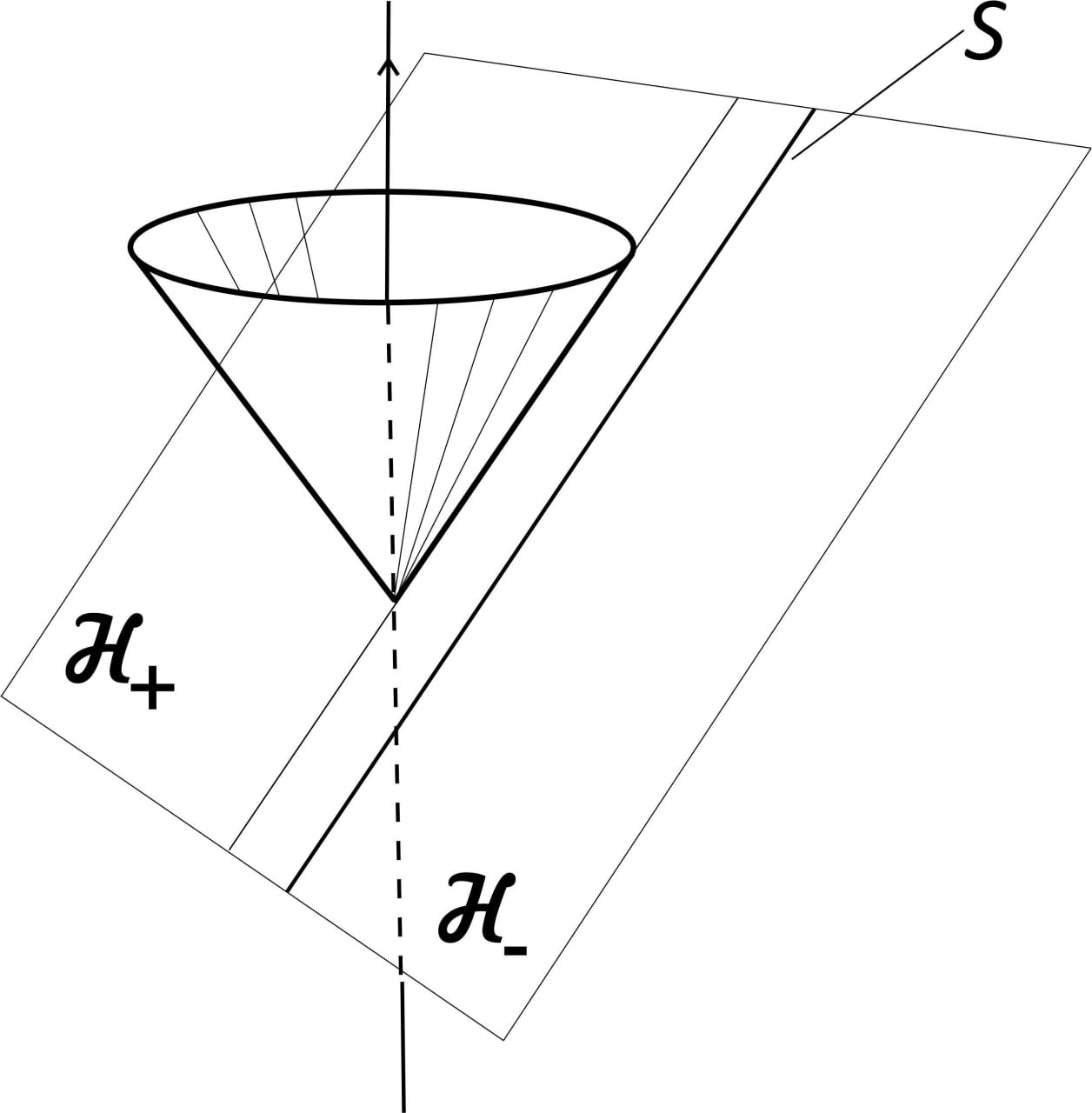
Figure 1: demonstrates the world-sheet of the string $\mathcal{S}$, the string horizon $\mathcal{H}=\mathcal{H}_{+}\cup\mathcal{H}_{-}$ and a trajectory of point-like mass (the dashed line) that crosses $\mathcal{H}_{+}$. At late times gravity waves generated by the string and the mass propagate along null cones $U=C$. Shown on the figure is the cone $U=0$ which is tangent to $\mathcal{H}$ and has the apex approximately at a point where the trajectory of the source crosses the horizon.

As we will see, solutions to problem (2.28)-(2.30) can be generated by a solution of the following scalar problem:

$$\Box\Phi_{\omega}(u,{\bf x})=0~{}~{},~{}~{}\Phi_{\omega}(0,{\bf x})=\theta(-y)~{}f_{\omega}({\bf x})~{}~{},$$ (3.2)

$$f_{\omega}({\bf x})\equiv f({\bar{\bf x}})~{}~{},~{}~{}f({\bf x})\equiv\phi(v/2,y,z)~{}~{}.$$ (3.3)

Here ${\bar{\bf x}}$ is defined in (2.19), and $\phi(x,y,z)$ in (2.23). The solution has a useful integral representation found in [15]:

$$\Phi_{\omega}(x)=-C\int_{S^{2}}d\Omega^{\prime}~{}\Re\left(\frac{\tilde{\Phi}_{\omega}(\Omega^{\prime})}{x\cdot m(\Omega^{\prime})+ia\varepsilon(\Omega^{\prime})}\right)~{}~{},~{}~{}\tilde{\Phi}_{\omega}(\Omega^{\prime})\equiv\frac{\cos\varphi^{\prime}}{g(\Omega^{\prime},\omega)}~{}~{}.$$ (3.4)

where $C=1/(8\pi^{3})$. The integration goes over a unit sphere $S^{2}$, with coordinates $\Omega^{\prime}=(\theta^{\prime},\varphi^{\prime})$, $d\Omega^{\prime}=\sin\theta^{\prime}d\theta d\varphi^{\prime}$. Other notations are:

$$m_{u}=1-\sin^{2}\theta^{\prime}\cos^{2}\varphi^{\prime}~{}~{} ,~{}~{}m_{v}=\sin^{2}\theta^{\prime}\cos^{2}\varphi^{\prime}~{}~{},$$

$$m_{y}=\sin 2\theta^{\prime}\cos\varphi^{\prime}~{}~{} ,~{}~{}m_{z}=\sin^{2}\theta^{\prime}\sin 2\varphi^{\prime}~{}~{},$$ (3.5)

$$g(\Omega^{\prime},\omega)=e^{i\theta^{\prime}}+\omega\sin\theta^{\prime}\cos\varphi^{\prime}~{}~{} ,~{}~{}\varepsilon(\Omega^{\prime})=2\sin^{2}\theta^{\prime}\cos\varphi^{\prime}~{}~{}.$$

One can check that vector field $m_{\mu}$ is null, $m^{2}=0$, which guarantees that $\Box\Phi_{\omega}=0$.

3.2 Exact form of perturbations and asymptotics

Boundary components of the metric of the source, which determine conditions (2.30), are

$$\hat{h}_{vv}({\bf x})=\frac{r_{g}}{2}f({\bf x})~{}~{},~{}~{}\hat{h}_{vi}({\bf x})=\hat{h}_{ij}({\bf x})=0~{}~{},~{}~{}i,j=y,z~{}~{},$$ (3.6)

$$\begin{split}\bar{h}_{vv}(u=0,{\bf x})=\frac{r_{g}}{2}\theta(-y)\bigl{(}f_{\omega}({\bf x})-f({\bf x})\bigr{)}~{}~{}&,~{}~{}\bar{h}_{yy}\mid_{\mathcal{H}_{-}}=2r_{g}\theta(-y)\omega^{2}f_{\omega}({\bf x})~{}~{},\\ \bar{h}_{vy}\mid_{\mathcal{H}_{-}}=-\omega r_{g}\theta(-y)f_{\omega}({\bf x})~{}~{}&,~{}~{}\bar{h}_{za}\mid_{\mathcal{H}_{-}}=0~{}~{},\end{split}$$ (3.7)

where $f({\bf x}),f_{\omega}({\bf x})$ are defined in (3.3). Equations (3.7) can be obtained with the help of (2.3).

Solution $\bar{h}_{ab}(x)$ to (2.28)-(2.30) can be expressed by using (3.2) as

$$\begin{split}\bar{h}_{vv}(x)=\frac{r_{g}}{2}\bigl{(}\Phi_{\omega}(x)-\Phi(x)\bigr{)}~{}~{}&,~{}~{}\bar{h}_{yy}(x)=2r_{g}\omega^{2}\Phi_{\omega}(x)~{}~{},\\ \bar{h}_{vy}(x)=-\omega r_{g}\Phi_{\omega}(x)~{}~{}&,~{}~{}\bar{h}_{za}(x)=0~{}~{},\end{split}$$ (3.8)

where $\Phi(x)=\Phi_{\omega=0}(x)$. With gauge conditions and Eqs. (3.8) one can construct other components $\bar{h}_{\mu\nu}$. As a result the string generated perturbations at $u>0$ can be represented in the following integral form:

$$h_{\mu\nu}(x)=-C\int_{S^{2}}d\Omega^{\prime}~{}\Re\left({\beta_{\mu\nu}(\Omega^{\prime})\over x\cdot m(\Omega^{\prime})+ia\varepsilon(\Omega^{\prime})}\right)~{}~{},$$ (3.9)

$$\beta_{\mu\nu}=\bar{\beta}_{\mu\nu}-\frac{1}{2}\eta_{\mu\nu}\bar{\beta}~{}~{},$$ (3.10)

$$\bar{\beta}_{vv} ={r_{g}\over 2}\bigl{(}\tilde{\Phi}_{\omega}-\tilde{\Phi}\bigr{)}~{}~{} ,~{}~{}\bar{\beta}_{vy} =-r_{g}\omega~{}\tilde{\Phi}_{\omega}~{}~{},$$ (3.11)

$$\bar{\beta}_{yy} =2r_{g}\omega^{2}~{}\tilde{\Phi}_{\omega}~{}~{} ,~{}~{}\bar{\beta}_{za} =0~{}~{}.$$ (3.12)

The gauge conditions are reduced to

$$m^{\mu}\bar{\beta}_{\mu\nu}=0~{}~{},$$ (3.13)

and allow one to find

$$\bar{\beta}_{ua}={1\over 2m_{v}}\bar{\beta}_{ab}~{}m^{b}~{}~{},~{}~{}\bar{\beta}_{uu}={1\over 4m^{2}_{v}}\bar{\beta}_{ab}~{}m^{a}m^{b}~{}~{}.$$ (3.14)

Equations (3.13) fix the components up to transformations ${\beta}_{\mu\nu}\to{\beta}_{\mu\nu}+a_{\mu}m_{\nu}+a_{\nu}m_{\mu}$, where $a^{\mu}m_{\mu}=0$. This freedom corresponds to some coordinate transformations which do not change (1.1) and the total radiated energy (1.2). The arbitrariness is eliminated, if $\beta_{ab}$ are required to be unchanged.

The subsequent analysis is based on arguments analogous to those of [16] for electromagnetic pulses caused by null strings. In coordinates $U,r,x^{A}$ the denominator in (3.9) can be written as

$$x^{\mu}m_{\mu}+ia\varepsilon=U+r\bigl{(}\vec{m}\cdot\vec{n}+1\bigr{)}+ia\varepsilon~{}~{},$$

where $\vec{n}=\vec{x}/r$, $x^{i}={x,y,z}$, is the unit vector defined above. We are interested in an asymptotic of (3.9) at large $r$. The integration in (3.9) can be decomposed into two regions: a domain, where the factor $(\vec{m}\cdot\vec{n})+1$ is small, that is, $\vec{m}$ is almost $-\vec{n}$ and the rest part of $S^{2}$. Let us introduce a dimensionless parameter $\Lambda$ such that

$${\sqrt{U^{2}+a^{2}}\over r}\ll\Lambda^{2}\ll 1~{}~{}.$$ (3.15)

We define the first region as $(\vec{m}\cdot\vec{n})+1\leq\Lambda^{2}$, and the second region as $(\vec{m}\cdot\vec{n})+1>\Lambda^{2}$ After some algebra one gets the following estimate (for components in the Minkowsky coordinates) for the first region:

$$h_{1,\mu\nu}(r,U,\Omega)\simeq{N(\Omega)\over r}\Re\left(\tilde{\beta}_{\mu\nu}\ln\left({U+ia\bar{\varepsilon}+r\Lambda^{2}\over U+ia\bar{\varepsilon}}\right)\right)~{}~{},$$ (3.16)

$$\tilde{\beta}_{\mu\nu}=\beta_{\mu\nu}\mid_{\vec{m}=-\vec{n}}~{}~{},~{}~{}\bar{\varepsilon}=\varepsilon\mid_{\vec{m}=-\vec{n}}~{}~{},$$ (3.17)

$$N(\Omega)=\frac{1}{4\pi^{2}}\sqrt{\frac{2}{1-n_{x}}}~{}~{}.$$ (3.18)

The leading large $r$ approximation in the second region can be easily computed

$$h_{2,\mu\nu}(r,U,\Omega)\simeq{b_{2,\mu\nu}(\Omega,\Lambda)\over r}~{}~{},~{}~{}b_{2,\mu\nu}(\Omega,\Lambda)=-C\int_{S^{2}_{\Lambda}}d\Omega^{\prime}~{}\Re\left({\beta_{\mu\nu}(\Omega^{\prime})\over\vec{n}\cdot\vec{m}(\Omega^{\prime})+1}\right)~{}~{}.$$ (3.19)

Here $S^{2}_{\Lambda}$ is a part of $S^{2}$ with the restriction $(\vec{m}\cdot\vec{n})+1>\Lambda^{2}$. As a result of (3.16), (3.19) the solution at large $r$ is a sum of a static, $h_{s,\mu\nu}$, and a time-dependent or dynamical, $h_{d,\mu\nu}$, parts:

$$h_{H,\mu\nu}(r,U,\Omega)\simeq h_{1,\mu\nu}+h_{2,\mu\nu}=h_{s,\mu\nu}+h_{d,\mu\nu}~{}~{},$$ (3.20)

$$h_{s,\mu\nu}(r,U,\Omega) \simeq{b_{\mu\nu}(\Omega,\Lambda)\over r} ,~{}~{}b_{\mu\nu}(\Omega,\Lambda) =N(\Omega)~{}\Re~{}\tilde{\beta}_{\mu\nu}(\Omega)\ln(r/\varrho)+b_{2,\mu\nu}(\Omega,\Lambda)~{}~{},$$ (3.21)

$$h_{d,\mu\nu}(r,U,\Omega) \simeq{H_{\mu\nu}(U,\Omega)\over r}~{} ,~{}H_{\mu\nu}(U,\Omega) =N(\Omega)~{}\Re\left(\tilde{\beta}_{\mu\nu}\ln\left({U+ia\bar{\varepsilon}\over a}\right)\right)~{}~{},$$ (3.22)

where $\varrho=a/\Lambda^{2}$. It is the dynamical part which contributes to the energy flux.

4 Calculating the flux of gravity waves

4.1 Polyhomogeneous space-times

According to Eqs. (2.14), (2.15) the metric of space-time sourced by the mass and the straight null string in the linear approximation has the form:

$$g^{\mbox{\tiny{out}}}_{\mu\nu}\simeq\eta_{\mu\nu}+h^{(1)}_{\mu\nu}~{}~{},~{}~{}h^{(1)}_{\mu\nu}=\hat{h}_{\mu\nu}+h_{\mu\nu}~{}~{}.$$ (4.1)

It has been shown in the previous section that perturbations at the future null infinity have the following asymptotic (in Minkowsky coordinates):

$$h^{(1)}_{\mu\nu}(r,U,\Omega)\simeq r^{-1}\Bigl{(}H^{(1)}_{\mu\nu}(U,\Omega)+\ln(r/\varrho)~{}\tilde{H}^{(1)}_{\mu\nu}(\Omega)\Bigr{)}+O(r^{-2}\ln r)~{}~{}~{}.$$ (4.2)

The gravitational field of the source yields a static ($U$ independent) contribution to $H^{(1)}_{\mu\nu}(U,\Omega)$. The gauge conditions in (2.16) impose constraints on the amplitudes. According to Eqs. (3.21), (3.22) the dynamical, $H^{(1)}_{\mu\nu}(U,\Omega)$, and static, $\tilde{H}^{(1)}_{\mu\nu}(\Omega)$, amplitudes depend on the complex tensor $\tilde{\beta}_{\mu\nu}(\Omega)$ defined in (3.17). Equations (3.13) and (3.17) imply the constraints related with the gauge conditions:

$$\bar{m}^{\mu}\left(\tilde{\beta}_{\mu\nu}-\frac{1}{2}\eta_{\mu\nu}\tilde{\beta}\right)=0~{}~{},$$ (4.3)

where $\bar{m}$ is a past-directed null vector with components $\bar{m}^{0}=-1,\vec{m}=-\vec{n}$. This vector is nothing but a null normal of the light cone $U=0$, see Fig. 1. That is, $m_{\mu}\sim\delta^{U}_{\mu}$. In coordinates (3.1) consequences of (3.21), (3.22) and (4.3) are

$$H^{(1)}_{r\nu}-\frac{1}{2}\eta_{r\nu}H^{(1)}=0~{}~{},~{}~{}\tilde{H}^{(1)}_{r\nu}-\frac{1}{2}\eta_{r\nu}\tilde{H}^{(1)}=0~{}~{},$$ (4.4)

$$H^{(1)}_{rr}=H^{(1)}_{rA}=\gamma^{AB}H^{(1)}_{AB}=0~{}~{},~{}~{}\tilde{H}^{(1)}_{rr}=\tilde{H}^{(1)}_{rA}=\gamma^{AB}\tilde{H}^{(1)}_{AB}=0~{}~{},$$ (4.5)

where $\gamma_{AB}$ is the metric on a unit 2-sphere. We can readily conclude that the spherical part, $C_{AB}(U,\Omega)\equiv H^{(1)}_{AB}(U,\Omega)$, which appears in (1.1), can be interpreted as the strain tensor of an outgoing gravitational wave which carries two polarizations.

Asymptotic (4.2), however, is not ”standard” due to the presence of the logarithmic terms with amplitude $\tilde{H}^{(1)}_{\mu\nu}(\Omega)$. Such space-times are called asymptotically polyhomogeneous space-times [23]. Their key property is in non-analytical behavior at conformal null infinities, see e.g. [29, 30, 31, 32, 33, 34]. The logarithmic terms result in the corresponding modification of the peeling properties of the curvature invariants [24]. Indeed, a straightforward calculation of one of the components of the Weyl tensor yields

$$C_{~{}~{}rBr}^{A}\simeq{1\over 2r^{3}}(\tilde{H}^{(1)})^{A}_{B}~{}~{},$$ (4.6)

where in the right hand side index $A$ is risen with the help of metric on the unit sphere. Eq. (4.6) means that for the polyhomogeneous space-times curvature invariant $\Psi_{0}$ behaves at large $r$ as $1/r^{3}$, see [29], in contrast with the standard peeling behavior which dictates a more rapid decay, as $1/r^{5}$.

The logarithmic terms in (4.2) result in static tidal forces. For instance, a test massive particle, which is at rest at a distance $r$ with respect to the considered source, acquires an additional constant coordinate acceleration with components $\delta w^{r}\sim r^{-2}\ln r~{}\tilde{H}_{UU}$, $\delta w^{A}\sim r^{-3}\ln r~{}(\tilde{H}_{UU})^{,A}$. Hence, a distance $L$ between two nearby test particles changes after a time $T$ by $\delta L\sim L~{}r^{-3}\omega r_{g}T^{2}\ln r$.

4.2 Going beyond the linearized approximation

We analyze now the energy carried away by gravity waves in case of this sort of polyhomogeneous space-times. To this aim one needs to go beyond the linearized approximation and write

$$g^{\mbox{\tiny{out}}}_{\mu\nu}\simeq\eta_{\mu\nu}+h^{(1)}_{\mu\nu}+h^{(2)}_{\mu\nu}~{}~{},$$ (4.7)

instead of (4.1). Second order correction $h^{(2)}_{\mu\nu}$ is determined by the Einstein equations

$$G_{\mu\nu}=\frac{1}{2}\kappa T_{\mu\nu}~{}~{},$$ (4.8)

where $T_{\mu\nu}$ is the stress-energy tensor of the source which first appeared in (2.24). By taking into account the linearized equations for $h^{(1)}_{\mu\nu}$ one gets from (4.8)

$$G^{(1)}_{\mu\nu}(h^{(2)})=-G^{(2)}_{\mu\nu}(h^{(1)})\equiv\frac{1}{2}\kappa t_{\mu\nu}~{}~{},$$ (4.9)

where $G^{(k)}$ is a term in decomposition of the Einstein tensor $G_{\mu\nu}$ over the flat metric which contains $k$-th power of $h^{(1)}$. The quantity $t_{\mu\nu}$ is the pseudo-tensor of the gravitational field. It is divergence free, $\partial^{\mu}t_{\mu\nu}=0$, since $\partial^{\mu}G^{(1)}_{\mu\nu}=0$. The energy flow is determined by $t^{r}_{U}$.

We proceed with computations in the harmonic gauge, $\partial^{\mu}\bar{h}^{(1)}_{\mu\nu}=\partial^{\mu}\bar{h}^{(2)}_{\mu\nu}=0$. Then the left and right sides of (4.9) are:

$$(G^{(1)})^{r}_{U}(h^{(2)})=-\frac{1}{2}\Box(h^{(2)})^{r}_{U}=\\ =-\frac{1}{2}\left(\partial_{r}^{2}-2\partial_{U}\partial_{r}-{2\over r}(\partial_{U}-\partial_{r})+{1\over r^{2}}(\eth_{A}\eth^{A}-2)\right)(h^{(2)})^{r}_{U}+{1\over r^{3}}\eth^{A}h^{(2)}_{UA}~{}~{},$$ (4.10)

$$-(G^{(2)})^{r}_{U}(h^{(1)})=\frac{1}{4}\Bigl{(}\partial_{U}(h^{(1)})^{AB}\partial_{U}(h^{(1)})_{AB}-\partial^{2}_{U}\bigl{(}(h^{(1)})^{AB}(h^{(1)})_{AB}\bigr{)}\Bigr{)}~{}~{},$$ (4.11)

where $\eth_{A}$ is the covariant derivative on $S^{2}$. We now suppose that $h^{(2)}$ has asymptotic behavior

$$h^{(2)}_{\mu\nu}(r,U,\Omega)\simeq r^{-1}\Bigl{(}H^{(2)}_{\mu\nu}(U,\Omega)+\ln(r/\varrho)~{}\tilde{H}^{(2)}_{\mu\nu}(U,\Omega)+\\ +\ln^{2}(r/\varrho)~{}\tilde{Q}^{(2)}_{\mu\nu}(U,\Omega)\Bigr{)}+O(r^{-2}\ln^{2}r)~{}~{}.$$ (4.12)

The differences between (4.2) and asymptotic (4.12) are the following: i) we admit possibility of higher order powers of the logarithms [29, 30, 31, 32, 33, 34], ii) we do not require that amplitudes $\tilde{H}^{(2)}$, $\tilde{Q}^{(2)}$ are static. Also note that conditions (4.4), (4.5) are not to be applicable to $H^{(2)}$, $\tilde{H}^{(2)}$, $\tilde{Q}^{(2)}$. One can show that the harmonic gauge conditions imply only time independence of some components

$$\partial_{U}H^{(2)}_{r\mu}=\partial_{U}\tilde{H}^{(2)}_{r\mu}=\partial_{U}\tilde{Q}^{(2)}_{r\mu}=0~{}~{}~{},~{}~{}\mu=r,A~{}~{},$$ (4.13)

$$\partial_{U}(\gamma^{AB}H^{(2)}_{AB})=\partial_{U}(\gamma^{AB}\tilde{H}^{(2)}_{AB})=\partial_{U}(\gamma^{AB}\tilde{Q}^{(2)}_{AB})=0~{}~{}~{}.$$ (4.14)

Substitution of (4.2) in (4.11) and (4.12) in (4.10) yields:

$$(G^{(1)})^{r}_{U}(h^{(2)})\simeq{1\over r^{2}}\partial_{U}(\tilde{H}^{(2)})^{r}_{U}+{2\over r^{2}}\partial_{U}(\tilde{Q}^{(2)})^{r}_{U}~{}\ln(r/\varrho)+O(r^{-3}\ln^{2}r)~{}~{},$$ (4.15)

$$t^{r}_{U}\simeq{2\over\kappa r^{2}}\Bigl{(}N_{AB}N^{AB}-\partial_{U}(C_{AB}N^{AB})-\partial_{U}(\tilde{H}^{(1)}_{AB}~{}N^{AB})\ln(r/\varrho)\Bigr{)}+O(r^{-3}\ln^{2}r)~{}~{},$$ (4.16)

where $N_{AB}\equiv\frac{1}{2}\partial_{U}C_{AB}$ and indices $A,B$ are now risen with the metric on unit $S^{2}$. From Eq. (4.9) one comes to relations between 1-st order and 2-d order perturbations in (4.7)

$$\partial_{U}(\tilde{H}^{(2)})^{r}_{U}=-N_{AB}N^{AB}+\partial_{U}(C_{AB}N^{AB})~{}~{},$$ (4.17)

$$2\partial_{U}(\tilde{Q}^{(2)})^{r}_{U}=\partial_{U}(\tilde{H}^{(1)}_{AB}~{}N^{AB})~{}~{}.$$ (4.18)

Equation (4.18) justifies inclusion the $\ln^{2}r$-term in (4.12). It is interesting to note that in the harmonic gauge only the logarithmic terms in $h^{(2)}_{\mu\nu}$ are responsible for the flux of gravity waves.

4.3 Intensity of the gravitational radiation

The stress-energy pseudo-tensor $t^{\mu}_{\nu}$ depends on the chosen gauge and it does not describe any localized energy. The physical meaning can be attributed to the global energy obtained by integrating $t^{0}_{0}$ over a space-like hypersurface. This integrated quantity should be invariant under coordinate transformations which preserve the leading asymptotic of the metric, see e.g. [35]. We demonstrate this property in Appendix B for $t^{r}_{U}$ component.

Consider the integrated energy in a ball $r\leq R$ of sufficiently large radius $R$. The change of the energy with time is given by the energy flux through the spherical boundary

$$W(U,R)=\int_{r=R}d\Omega~{}r^{2}~{}t^{r}_{U}(r,U,\Omega)~{}~{}.$$ (4.19)

This quantity is certainly not finite in the limit $R\to\infty$ due to the presence of the logarithmic term in r.h.s. of (4.16). To understand whether this divergence is physically relevant one needs to calculate the energy

$$E(U_{2},U_{1},R)=\int_{U_{1}}^{U_{2}}dU~{}W(U,R)~{}~{},$$ (4.20)

emitted over a period of time $U_{2}-U_{1}\equiv\Delta U$ ($U_{2}>0$, $U_{1}<0$) much larger than a typical wave-length of the system. Since the impact parameter $a$ can be interpreted as a ”size” of the system (the string and the mass), which determines a duration of the gravitational pulse and an effective wave-length of the emitted radiation, one needs $\Delta U\gg a$.

When integrating $t^{r}_{U}$ over $U$ contributions of the last two terms in r.h.s. of (4.16) are suppressed at $|U|\gg a$ as a result of the following asymptotics:

$$C_{AB}N^{AB}\sim U^{-1}\ln(|U|/a)~{}~{},~{}~{}\tilde{H}^{(1)}_{AB}~{}N^{AB}~{}\ln(r/\varrho)\sim U^{-1}\ln(r/\varrho)~{}~{}.$$ (4.21)

Let us remind that our approximation is obtained under assumption (3.15) which implies that $|U|\ll R$. If one puts $U_{i}=c_{i}R$, where $c_{i}$ are some constants, $|c_{i}|\ll 1$, $c_{2}>0$, $c_{1}<0$, and takes into account (4.21) the total radiated energy $E$ defined below does not depend on the logarithmic terms at large $R$ and takes the form

$$E=\lim_{R\to\infty}E(c_{2}R,c_{1}R,R)={2\over\kappa}\int_{-\infty}^{\infty}dU\int d\Omega~{}N_{AB}N^{AB}~{}~{}.$$ (4.22)

We conclude that the logarithmic divergence in the flux disappears when averaging the radiated energy on time intervals much larger than the impact parameter $a$. So the divergence is irrelevant.

In a similar way we define an averaged intensity of the flux as

$$I(\Omega)\equiv{1\over a}\lim_{R\to\infty}\int_{c_{1}R}^{c_{2}R}dU~{}R^{2}~{}t^{r}_{U}(R,U,\Omega)={2\over a\kappa}\int_{-\infty}^{\infty}dU~{}N_{AB}N^{AB}~{}~{}.$$ (4.23)

Relation between the averaged intensity and the total emitted energy is

$$E=a\int d\Omega~{}I(\Omega)~{}~{}.$$ (4.24)

Straightforward but tedious computations presented in Appendix A yield:

$$I(\Omega)=\frac{\pi N(\Omega)^{2}}{4\kappa\bar{\varepsilon}(\Omega)}\left(\alpha(\Omega)+\frac{\gamma(\Omega)}{a^{2}\bar{\varepsilon}^{2}(\Omega)}\right)~{}~{},$$ (4.25)

where $N$ is defined in (3.18), $\bar{\varepsilon}$ in (A.5) and $\alpha$, $\gamma$ in (A.13), (A.15).

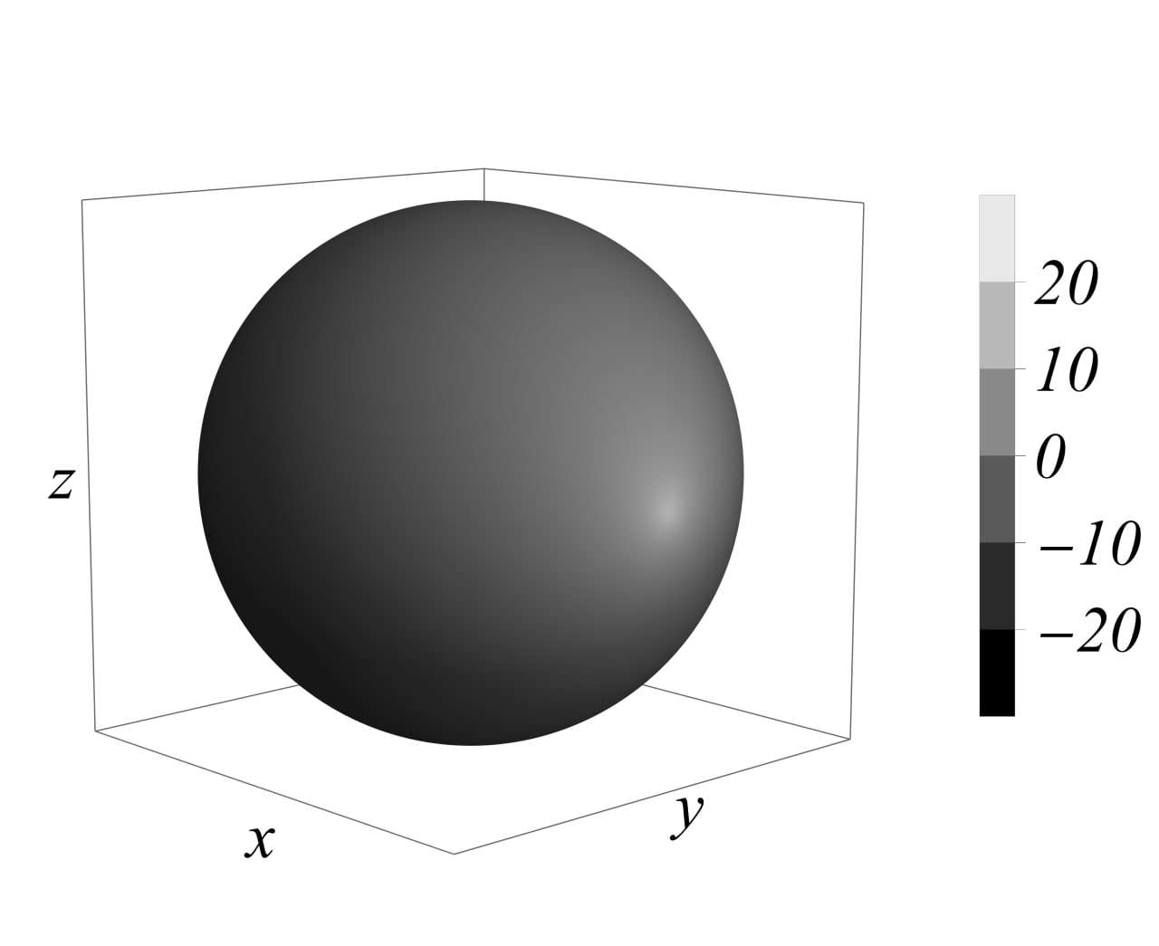
Figure 2: shows the angular distribution of the logarithm of the averaged intensity of the generated gravitational radiation. The intensity is concentrated in the direction of the string motion, on the axis $y=z=0$.

Angular distribution of the logarithm of the intensity is shown on Fig. 2. The picture looks similar to the case of electromagnetic radiation generated by a straight null string and an electric of magnetic-dipole point-like source. The intensity is concentrated near the line which goes through the source parallel to the velocity of the string and in the direction of the string motion.

Let us emphasize that we present $I(\Omega)$ just to give a qualitative picture of the angle distribution of the gravitational radiation. We do not discuss in the present work more physically interesting characteristics, such as, for example, response of gravitational detectors to string generated gravitational waves.

4.4 Deformation of the string and displacement of the source

The results obtained for metric perturbations imply that position of the source is fixed and the string is straight. In reality, the source and each point of the string move along their geodesics in a weak gravitational field. Changes in the position of the source and in the form of the string may affect the analysis given above. To estimate possible corrections, we assume that each small section of the string contributes independently to the metric perturbation.

Let $a_{0}+\delta a$ be an impact parameter of a given section, where $a_{0}$ is an impact parameter of the section for straight string and initial position of the source. An addition $\delta a$ appears due to the deformation of the string and the displacement of the source. If $\delta a/a_{0}$ is small for each segment of the string, then correction to the perturbation of the metric should be suppressed by factor $O(\max(\delta a/a_{0}))$ as compared to the main effect.

The interaction of the string with the source takes an infinite time, so $\delta a$ even in the weak gravitational field of the source can be infinitely large. However, the flux of gravitational radiation, determined by $N_{AB}N^{AB}$, describes the gravitational burst at moments $U\sim O(a)$. Since $\delta a$ during this time are expected to be of order $r_{g}$ (see explicit calculations in [8]), the relative correction for the contribution of the each section of the string, and, accordingly, of the entire string, is suppressed by factor $O(r_{g}/a)$. This effect is small enough to be neglected.

As for the displacement of the source under the action of the gravity wave, the acceleration of the source can be estimated as $\omega r_{g}/a^{2}$. During a time interval $\Delta U=O(a)$ the source may be moved at a distance not larger than $O(\omega r_{g})$. This displacement is extremely small and does not affect our results as well.

4.5 Averaged luminosity and spin effects

Let us estimate now the averaged luminosity of the flux, which can be crudely defined as:

$$\dot{E}\equiv{E\over a}\sim~{}C~{}\frac{\omega^{2}}{a^{2}}~{}\frac{r_{g}^{2}}{G}~{}~{},$$ (4.26)

where $C$ is a numerical coefficient, $C<O(10^{-2})$ and $r_{g}=2MG$ is the gravitational radius of the source. For tensile cosmic strings with tension $\mu$ the CMB spectrum yields the constraint $G\mu\leq 10^{-7}$, see [37, 38, 39], while the stochastic gravitational-wave background gives a stronger limit, $G\mu\leq 10^{-12}$, see [1].

Since we are dealing with gravitational radiation the parameter $\omega_{0}=1\cdot 10^{-12}$ can be used as some reference value, and (4.26) can be rewritten as

$$\dot{E}\sim~{}C\left({\omega\over\omega_{0}}\right)^{2}\left({r_{g}\over a}\right)^{2}\cdot 10^{36}~{}{\mbox{erg}\over\mbox{s}}~{}~{}.$$ (4.27)

Thus, a null string and a massive source with impact parameter $a=10~{}r_{g}$ and $\omega\sim\omega_{0}$ have the luminosity of the order $10^{34}$ erg per second, which is comparable with gravity wave luminosity of such systems as the double pulsar PSR B1913+16. Yet such luminosity is extremely smaller than the peak luminosity of gravitational radiation produced by binary black hole mergers (about $10^{56}$ erg per second).

If the source has a spin $J_{j}$ there will be non-trivial components in Eq. (2.22)

$$\hat{h}_{0i}=4G~{}\varepsilon_{ijk}J_{j}\partial_{k}\phi~{}~{},$$ (4.28)

where $i,j,k$ correspond $x,y,z$. These components yield additional contributions to string generated gravity waves. As a result one expects two additions to (4.27): one is due to the radiated energy $E_{mJ}$ proportional to mass $m$ of the source and spin $J$, another, $E_{J}$, is of the second order in $J$. By taking into account that spin factors may appear in the dimensionless combination $GJ/a^{2}$ it is easy to come to the following estimates:

$$\dot{E}_{mJ} \sim~{}\dot{E}\left({a\over r_{g}}\right)\left({GJ\over a^{2}}\right)~{}~{},$$ (4.29)

$$\dot{E}_{J} \sim~{}\dot{E}\left({a\over r_{g}}\right)^{2}\left({GJ\over a^{2}}\right)^{2}~{}~{}.$$ (4.30)

Suppose the source is a Kerr black hole. In this case one can introduce the black hole parameter $a_{bh}=J/M$, such that the black hole is extremal if $a_{bh}=MG$. Relations (4.29), (4.30) can be transformed as follows:

$$\dot{E}_{mJ} \sim~{}\dot{E}\left({a_{bh}\over a}\right)~{}~{},$$ (4.31)

$$\dot{E}_{J} \sim~{}\dot{E}\left({a_{bh}\over a}\right)^{2}~{}~{}.$$ (4.32)

Thus, contributions to the luminosity from the spin are suppressed by factors of $a_{bh}/a<r_{g}/a$, as compared to the luminosity due to the mass of the source. One can neglect spin effects in crude estimates of the luminosity.

4.6 Detection of string generated gravity waves

As it follows from Eqs. (3.20)-(3.22) the amplitude of a gravitational wave outgoing from the string and a source has the order of magnitude $h\sim\omega r_{g}/r$. Earth-based gravitational antenna have the sensitivity to gravity waves with wave lengths in the interval $50-500~{}$km and amplitude $\sim 10^{-21}$. Thus, the impact parameter $a$ of our system has to be of the same order, and the most suitable sources to produce gravity waves from moving null strings are stellar mass black holes with $r_{g}\sim 1~{}$km. For $\omega=O(10^{-12})$ and a black hole located in a nearby galaxy, say, in the Andromeda Galaxy (M31), with the distance to the Earth about $r\sim 1~{}\mathrm{Mpc}\sim 10^{19}~{}$km, the amplitude of the gravity wave would be $\sim 10^{-31}$, too small to be detected. Gravity waves can be also observed by possible space-based interferometers. For supermassive black holes the waves generated by null strings have much larger amplitudes, but they are still very small to be observed. Therefore, direct registration of signals produced by null cosmic strings from massive sources is a challenging task.

If exist, the null cosmic strings, when moving through the matter distributed over the Universe, produce numerous gravity waves of different wave lengths at different epochs. All these waves contribute to a stochastic gravitational wave background (SGWB). Detection of SGWB and understanding its sources is one of the important purposes of gravitational wave experiments, see [40] for a review.

In addition to compact massive sources, such as black holes and neutron stars, the Universe may contain clumps of cold dark matter (DM). Within existing models [41, 42], small clumps can have masses up to thousands of solar masses and sizes up to few parsecs, with a diverse density profiles, from a density of the order of $M_{\odot}\,\mathrm{pc}^{-3}$ to a density in the core comparable to the neutron star density. Detection of such small clumps by microlensing is difficult, so the possibilities of detecting gravitational wave signals from clumps are being actively explored, both using detectors such as LISA, LIGO [43], and by using pulsar timings [41].

Gravitational responses of detectors or pulsars when a clump of DM passes nearby, as well as GW effects caused by clump fragmentation can be significant [44]. The above analysis of string generated gravity waves from point sources can be generalized to the case of GW from compact or fairly sparse clumps of DM. Since such waves should contribute to SGWB, their effects may provide another theoretical possibility for detecting the dark matter.

Below we estimate gravitational effects from a string and a DM clump of mass $M$ which is uniformly distributed over a spatial domain with a characteristic size $L$. As earlier, we assume that the string is straight. By using (3.22) and assuming that $r\gg L$ one gets for the news tensor

$$N_{AB}\simeq N(\Omega)~{}\Re\left(\tilde{\beta}_{AB}(\Omega)\int_{a}^{a+L}{\rho~{}dy\over U(y)+iy\bar{\varepsilon}}\right)~{}~{}.$$ (4.33)

Here integration goes over a section of the clump by the plane of constant $x$ and $z$, $\rho\sim M/L$ is a mass density of this section, and $a$ now is a least impact parameter between points of the clump and the string. It follows from (4.33) that the parameter $r_{g}/a$, which determines the amplitude of the news tensor for a point-like mass, should be replaced with the ratio $GM/L$, if the clump is sufficiently homogeneous and it does not cross the string. This means that for the case of the clump our estimate (4.26) should be replaced with

$$\dot{E}\equiv{E\over L}\sim~{}C\left({\omega\over\omega_{0}}\right)^{2}\left({r_{g}\over L}\right)^{2}\cdot 10^{36}~{}{\mbox{erg}\over\mbox{s}}~{}~{}.$$ (4.34)

For $M\sim 10^{3}M_{\odot}$, $L\sim 1$ pc, $\omega\sim\omega_{0}$, one has $\dot{E}\sim 10^{15}$ erg per second. Since the effective frequency of the radiation with such parameters is in the nanohertz range, its detection is possible by using pulsar timings.

5 Concluding remarks

The aim of this work was two-fold. First, we were going to check if the description of field effects in null-string space-times [15] can be extended to weak gravitational fields. Second, we were looking for gravitational effects which could provide potential observational signatures of null cosmic strings.

To our knowledge, our result is the first solution in the linearized approximation for the space-time geometry sourced by a point mass and a null string. The solution is not stationary and asymptotically non-trivial. Since it belongs to a class of polyhomogeneous space-times calculating the flux of outgoing gravity waves requires some care. As has been shown non-analytic terms in the flux can be eliminated by averaging over a sufficiently large period of time.

One difficulty, which appears when dealing with polyhomogeneous space-times, is that the Bondi analysis of the gravitational radiation based on the mass aspect, see e.g. [36], cannot be applied here straightforwardly. It should be emphasized that coordinates $x^{\mu}=(U,r,\Omega)$ we use here and the Bondi-Sachs coordinates are different and should not be confused. We work in the harmonic gauge, while the Bondi-Sachs coordinates are determined by the conditions $g_{rr}=g_{rA}=0$ and $\det g_{AB}=r^{4}\sin^{2}\theta$. These conditions hold only for $h^{(1)}$ up to $O(r^{-2})$ terms , see (4.5), and they are violated for higher order perturbations starting with $h^{(2)}$. It would be interesting to identify the mass aspect function for the considered geometry.

The luminosity generated by null strings in the form of gravitational radiation is much higher than the luminosity generated in the form of electro-magnetic (EM) radiation. For example, according to (4.27), for the string energy parameter $\omega\sim 10^{5}\omega_{0}$ the GW luminosity of a null string and a pulsar is $10^{46}$ erg per second against $10^{28}$ erg per second of the EM luminosity of the same system, see [16]. Thus, we expect that the generated gravitational radiation can be important source of data to identify possible signatures of null cosmic strings. We are going to proceed with a more careful analysis of contribution from null strings to SGWB, by analogy with contribution from tensile cosmic strings.

As we have mentioned in Section 4.5 spin effects related to the rotation of the source can be neglected in the averaged luminosity. In case of EM radiation generated by a null string near a magnetic-dipole source the intensity depends on orientation of the magnetic moment of the source [16]. Thus, one may expect that intensity of gravity waves may be sensitive to mutual orientation of the spin of the source and velocity of the string. It would be interesting to study these effects in a separate work.

Our arguments in Section 4.4 to demonstrate that the obtained results are robust have been based on assumption that each segment of the string contributes independently to the flux. There is one effect, which cannot be described in terms of individual contributions of string sections. This happens when a null string forms a caustic behind the source at a distance $a^{2}/2r_{g}$, see [8]. Since a large amount of energy is concentrated in a domain around the caustic, it may create its own gravity waves. If this effect does exist its properties are expected to be quite different from gravity waves we consider in this work.

6 Acknowledgments

This research is supported by Russian Science Foundation grant No. 22-22-00684.

Appendix A Computations

Here we give some details of how explicit form of asymptotic (4.2) looks like. One starts with Eq. (3.9) where tensor $\beta_{\mu\nu}$ has the following components:

$$\begin{split}\beta_{uu}&=\frac{r_{g}}{2}\biggl{(}\left(\frac{m_{u}+\omega m_{y}}{m_{v}}\right)^{2}\tilde{\Phi}_{\omega}-\left(\frac{m_{u}}{m_{v}}\right)^{2}\tilde{\Phi}\biggr{)}~{}~{},\\ \beta_{uv}&=\frac{r_{g}}{2}~{}\omega^{2}\tilde{\Phi}_{\omega}~{}~{},\\ \beta_{uy}&=r_{g}~{}\omega~{}\frac{m_{u}+\omega m_{y}}{m_{v}}\tilde{\Phi}_{\omega}~{}~{},\\ \beta_{vv}&=\frac{r_{g}}{2}\bigl{(}\tilde{\Phi}_{\omega}-\tilde{\Phi}\bigr{)}~{}~{},\\ \beta_{vy}&=-r_{g}\omega\tilde{\Phi}_{\omega}~{}~{},\\ \beta_{yy}&=r_{g}\biggl{(}-\frac{(m_{u}+\omega m_{y}-\omega^{2}m_{v})}{m_{v}}\tilde{\Phi}_{\omega}+\frac{m_{u}}{m_{v}}\tilde{\Phi}\biggr{)}~{}~{},\\ \beta_{zz}&=r_{g}\biggl{(}-\frac{(m_{u}+\omega m_{y}+\omega^{2}m_{v})}{m_{v}}\tilde{\Phi}_{\omega}+\frac{m_{u}}{m_{v}}\tilde{\Phi}\biggr{)}~{}~{},\\ \beta_{uz}&=\beta_{vz}=\beta_{yz}=0~{}~{}.\end{split}$$ (A.1)

Amplitude $H^{(1)}_{\mu\nu}$ is determined from Eq. (3.22) as

$$H^{(1)}_{\mu\nu}(U,\Omega)=N(\Omega)~{}\Re\left(\tilde{\beta}_{\mu\nu}\ln\left({U+ia\bar{\varepsilon}\over a}\right)\right)~{}~{}.$$ (A.2)

As has been explained in Sec. 3.2 tensor structures $\tilde{\beta}_{\mu\nu}$ are values of $\beta_{\mu\nu}$ when null vector $m^{\mu}$ is a normal vector to the null cone $U=0$, see (3.17). A straightforward computation yields

$$\begin{split}\tilde{\beta}_{uu}&=\frac{r_{g}}{2}\biggl{(}\left(\frac{1+n_{x}-2\omega n_{y}}{1-n_{x}}\right)^{2}\tilde{\phi}_{\omega}-\left(\frac{1+n_{x}}{1-n_{x}}\right)^{2}\tilde{\phi}\biggr{)}~{}~{},\\ \tilde{\beta}_{uv}&=\frac{r_{g}}{2}\omega^{2}\tilde{\phi}_{\omega}~{}~{},\\ \tilde{\beta}_{uy}&=r_{g}\omega\frac{1+n_{x}-2\omega n_{y}}{1-n_{x}}\tilde{\phi}_{\omega}~{}~{},\\ \tilde{\beta}_{vv}&=\frac{r_{g}}{2}\bigl{(}\tilde{\phi}_{\omega}-\tilde{\phi}\bigr{)}~{}~{},\\ \tilde{\beta}_{vy}&=-r_{g}\omega\tilde{\phi}_{\omega}~{}~{},\\ \tilde{\beta}_{yy}&=r_{g}\left(-\frac{(1+n_{x}-2\omega n_{y}-\omega^{2}(1-n_{x}))}{1-n_{x}}\tilde{\phi}_{\omega}+\frac{1+n_{x}}{1-n_{x}}\tilde{\phi}\right)~{}~{},\\ \tilde{\beta}_{zz}&=r_{g}\left(-\frac{(1+n_{x}-2\omega n_{y}+\omega^{2}(1-n_{x}))}{1-n_{x}}\tilde{\phi}_{\omega}+\frac{1+n_{x}}{1-n_{x}}\tilde{\phi}\right)~{}~{},\\ \tilde{\beta}_{uz}&=\tilde{\beta}_{vz}=\tilde{\beta}_{yz}=0~{}~{},\end{split}$$ (A.3)

where $\tilde{\phi}=\tilde{\phi}_{\omega=0}$ and

$$\tilde{\phi}_{\omega}=\frac{\sqrt{2}(1-n_{x})^{3/2}}{\bar{\varepsilon}\bigl{(}-n_{y}+\omega(1-n_{x})+i\bar{\varepsilon}\bigr{)}}~{}~{},$$ (A.4)

$$\bar{\varepsilon}=\sqrt{2(1-n_{x})-n_{y}^{2}}~{}~{}.$$ (A.5)

If the energy of the string is small, $\omega\ll 1$,

$$\begin{split}\tilde{\beta}_{uu}&\simeq-r_{g}\omega\frac{1+n_{x}}{2\sqrt{2}(1-n_{x})^{3/2}}\left(\frac{1}{\bar{\varepsilon}}\Bigl{(}n_{x}^{2}-1+n_{y}^{2}(n_{x}-3)\Bigr{)}+in_{y}(n_{x}-3)\right)+O(\omega^{2})~{}~{},\\ \tilde{\beta}_{uv}&\simeq 0+O(\omega^{2})~{}~{},\\ \tilde{\beta}_{uy}&\simeq-r_{g}\omega\frac{1+n_{x}}{\sqrt{2(1-n_{x})}}\left(\frac{n_{y}}{\bar{\varepsilon}}+i\right)+O(\omega^{2})~{}~{},\\ \tilde{\beta}_{vv}&\simeq r_{g}\omega\sqrt{\frac{1-n_{x}}{2}}\left(\frac{\bar{\varepsilon}^{2}-n_{y}^{2}}{4\bar{\varepsilon}}-i\frac{n_{y}}{2}\right)+O(\omega^{2})~{}~{},\\ \tilde{\beta}_{vy}&\simeq r_{g}\omega\sqrt{\frac{1-n_{x}}{2}}\left(\frac{n_{y}}{\bar{\varepsilon}}+i\right)+O(\omega^{2})~{}~{},\\ \tilde{\beta}_{yy}&\simeq-r_{g}\omega\sqrt{\frac{1-n_{x}}{2}}\left(\frac{1}{\bar{\varepsilon}}\bigl{(}n_{y}^{2}+n_{x}+1\bigr{)}+in_{y}\right)+O(\omega^{2})~{}~{},\\ \tilde{\beta}_{zz}&\simeq-r_{g}\omega\sqrt{\frac{1-n_{x}}{2}}\left(\frac{1}{\bar{\varepsilon}}\bigl{(}n_{y}^{2}+n_{x}+1\bigr{)}+in_{y}\right)+O(\omega^{2})~{}~{},\\ \tilde{\beta}_{uz}&=\tilde{\beta}_{vz}=\tilde{\beta}_{yz}=0~{}~{}.\end{split}$$ (A.6)

The averaged intensity of the radiation is

$$I(\Omega)=\frac{2}{a\kappa}\int_{-\infty}^{\infty}dUf_{G}(U,\Omega)~{}~{},$$ (A.7)

$$f_{G}(U,\Omega)\equiv N_{AB}N^{AB}~{}~{},~{}~{}N_{AB}=\frac{1}{2}\partial_{U}C_{AB}~{}~{}.$$ (A.8)

After some algebra, by using gauge conditions (4.3), one finds a useful expression in terms of components of $N_{\mu\nu}=\frac{1}{2}\partial_{U}H^{(1)}_{\mu\nu}$ in the Minkowsky coordinates:

$$f_{G}(U,\Omega)=A_{1}N_{vv}^{2}+A_{2}N_{vy}^{2}+A_{3}N_{yy}^{2}+A_{4}N_{zz}^{2}+A_{5}N_{vv}N_{vy}+\\ +A_{6}N_{vv}N_{yy}+A_{7}N_{vv}N_{zz}+A_{8}N_{vy}N_{yy}+A_{9}N_{vy}N_{zz}+A_{10}N_{yy}N_{zz}~{}~{},$$ (A.9)

$$A_{1} =(1-n_{x}^{2})^{2}~{}~{}, A_{6} =\frac{1}{2}\Bigl{(}4n_{y}^{2}-(3-n_{x})(1-n_{x})(1+n_{x})^{2}\Bigr{)}~{}~{},$$

$$A_{2} =\frac{8n_{z}^{2}+n_{y}^{2}(1-n_{x})^{4}}{(1-n_{x})^{2}}~{}~{}, A_{7} =\frac{1}{2}\Bigl{(}(1-n_{x})^{3}(1+n_{x})-4n_{y}^{2}\Bigr{)}~{}~{},$$

$$A_{3} =\frac{8n_{z}^{2}(3-n_{x})+(1-n_{x})^{5}}{16(1-n_{x})}~{}~{}, ~{}~{}~{}A_{8} =\frac{n_{y}}{2(1-n_{x})^{2}}\Bigl{(}4n_{z}^{2}(3-n_{x})+(1-n_{x})^{5}\Bigr{)}~{}~{},$$ (A.10)

$$A_{4} =\frac{8n_{y}^{2}(3-n_{x})+(1-n_{x})^{5}}{16(1-n_{x})}~{}~{}, A_{9} =\frac{n_{y}(n_{x}-3)}{2(1-n_{x})^{2}}\Bigl{(}4n_{z}^{2}+(1-n_{x})^{3}(1+n_{x})\Bigr{)}~{}~{},$$

$$A_{5} =2n_{y}(1-n_{x})(1-n_{x}^{2})~{}~{}, A_{10} =\frac{1}{8}(n_{x}-3)(1+n_{x})(1-n_{x})^{2}~{}~{}.$$

To proceed we decompose

$$\tilde{\beta}_{\mu\nu}=a_{\mu\nu}+i~{}b_{\mu\nu}~{}~{},$$ (A.11)

and find the following final expression:

$$f_{G}(U,\Omega)=\frac{a^{2}N(\Omega)^{2}}{4(U^{2}+a^{2}\bar{\varepsilon}^{2})^{2}}\Bigl{(}\alpha~{}U^{2}+\beta~{}U+\gamma\Bigr{)}~{}~{},$$ (A.12)

$$\alpha=A_{1}a_{vv}^{2}+A_{2}a_{vy}^{2}+A_{3}a_{yy}^{2}+A_{4}a_{zz}^{2}+A_{5}a_{vv}a_{vy}+\\ +A_{6}a_{vv}a_{yy}+A_{7}a_{vv}a_{zz}+A_{8}a_{vy}a_{yy}+A_{9}a_{vy}a_{zz}+A_{10}a_{yy}a_{zz}~{}~{},$$ (A.13)

$$\beta=a\bar{\varepsilon}\Bigl{(}2A_{1}a_{vv}b_{vv}+2A_{2}a_{vy}b_{vy}+2A_{3}a_{yy}b_{yy}+2A_{4}a_{zz}b_{zz}+\\ +A_{5}(a_{vy}b_{vv}+a_{vv}b_{vy})+A_{6}(a_{yy}b_{vv}+a_{vv}b_{yy})+A_{7}(a_{zz}b_{vv}+a_{vv}b_{zz})+\\ +A_{8}(a_{yy}b_{vy}+a_{vy}b_{yy})+A_{9}(a_{zz}b_{vy}+a_{vy}b_{zz})+A_{10}(a_{zz}b_{yy}+a_{yy}b_{zz})\Bigr{)}~{}~{},$$ (A.14)

$$\gamma=a^{2}\bar{\varepsilon}^{2}\Bigl{(}A_{1}b_{vv}^{2}+A_{2}b_{vy}^{2}+A_{3}b_{yy}^{2}+A_{4}b_{zz}^{2}+A_{5}b_{vv}b_{vy}+\\ +A_{6}b_{vv}b_{yy}+A_{7}b_{vv}b_{zz}+A_{8}b_{vy}b_{yy}+A_{9}b_{vy}b_{zz}+A_{10}b_{yy}b_{zz}\Bigr{)}~{}~{},$$ (A.15)

where

$$\begin{split}a_{vv}&=\frac{r_{g}}{2}(a_{\omega}-a_{0})~{}~{},\\ a_{vy}&=-r_{g}\omega a_{\omega}~{}~{},\\ a_{yy}&=r_{g}\left(-\frac{(1+n_{x}-2\omega n_{y}-\omega^{2}(1-n_{x}))}{1-n_{x}}a_{\omega}+\frac{1+n_{x}}{1-n_{x}}a_{0}\right)~{}~{},\\ a_{zz}&=r_{g}\left(-\frac{(1+n_{x}-2\omega n_{y}+\omega^{2}(1-n_{x}))}{1-n_{x}}a_{\omega}+\frac{1+n_{x}}{1-n_{x}}a_{0}\right)~{}~{},\end{split}$$ (A.16)

$$\begin{split}b_{vv}&=\frac{r_{g}}{2}(b_{\omega}-b_{0})~{}~{},\\ b_{vy}&=-r_{g}\omega b_{\omega}~{}~{},\\ b_{yy}&=r_{g}\left(-\frac{(1+n_{x}-2\omega n_{y}-\omega^{2}(1-n_{x}))}{1-n_{x}}b_{\omega}+\frac{1+n_{x}}{1-n_{x}}b_{0}\right)~{}~{},\\ b_{zz}&=r_{g}\left(-\frac{(1+n_{x}-2\omega n_{y}+\omega^{2}(1-n_{x}))}{1-n_{x}}b_{\omega}+\frac{1+n_{x}}{1-n_{x}}b_{0}\right)~{}~{},\end{split}$$ (A.17)

$$a_{\omega}=\Re~{}\tilde{\phi}_{\omega} =\frac{\sqrt{2(1-n_{x})}\bigl{(}-n_{y}+\omega(1-n_{x})\bigr{)}}{\bar{\varepsilon}\Bigl{(}2(1-\omega n_{y})+\omega^{2}(1-n_{x})\Bigr{)}}~{}~{},$$ (A.18)

$$b_{\omega}=\Im~{}\tilde{\phi}_{\omega} =\frac{-\sqrt{2(1-n_{x})}}{\Bigl{(}2(1-\omega n_{y})+\omega^{2}(1-n_{x})\Bigr{)}}~{}~{},$$ (A.19)

and also $a_{0}=a_{\omega=0},b_{0}=b_{\omega=0}$.

Appendix B Coordinate invariance of the averaged pseudo-tensor

Here we demonstrate that the averaged $t^{r}_{U}$-component of the pseudo-tensor (and, therefore, the averaged intensity of the GW flux) is invariant under general coordinate transformations which preserve asymptotic (4.2) but may violate gauge conditions (4.5). Thus the presence of logarithmic terms does not affect this important property.

The coordinate transformations are generated by a vector field $\xi^{\mu}$. We suppose that large $r$ asymptotic of the components of this vector in Minkowsky coordinates is

$$\xi^{\mu}=\alpha^{\mu}(\Omega)+\tilde{\alpha}^{\mu}(\Omega)\ln(r/\varrho)+r^{-1}\bigl{(}\sigma^{\mu}(U,\Omega)+\tilde{\sigma}^{\mu}(U,\Omega)\ln(r/\varrho)\bigr{)}+O(r^{-2}\ln r)~{}~{}.$$ (B.1)

Vectors $\alpha^{\mu}$, $\tilde{\alpha}^{\mu}$, $\sigma^{\mu}$, $\tilde{\sigma}^{\mu}$ are fairly arbitrary. We only require that components $\sigma^{\mu}$, $\tilde{\sigma}^{\mu}$ are restricted at $U\to\pm\infty$. After this transformation (4.2) can be written as follows:

$$h^{(1)^{\prime}}_{\mu\nu}=r^{-1}\Bigl{(}H_{\mu\nu}^{(1)}(U,\Omega)+\Xi_{\mu\nu}(U,\Omega)+\bigl{(}\tilde{H}_{\mu\nu}^{(1)}(\Omega)+\tilde{\Xi}_{\mu\nu}(U,\Omega)\bigr{)}\ln(r/\varrho)\Bigr{)}+O(r^{-2}\ln r)~{}~{},$$ (B.2)

$$\Xi_{UU} =2\partial_{U}\sigma_{U}~{}~{}, \tilde{\Xi}_{UU} =2\partial_{U}\tilde{\sigma}_{U}~{}~{},$$

$$\Xi_{Ur} =\partial_{U}\sigma_{r}+\tilde{\alpha}_{U}~{}~{}, \tilde{\Xi}_{Ur} =\partial_{U}\tilde{\sigma}_{r}~{}~{},$$

$$\Xi_{UA} =\partial_{A}\alpha_{U}+\partial_{U}\sigma_{A}~{}~{}, \tilde{\Xi}_{UA} =\partial_{A}\tilde{\alpha}_{U}+\partial_{U}\tilde{\sigma}_{A}~{}~{},$$ (B.3)

$$\Xi_{rr} =2\tilde{\alpha}_{r}~{}~{}, \tilde{\Xi}_{rr} =0~{}~{},$$

$$\Xi_{rA} =\partial_{A}\alpha_{r}-\alpha_{A}+\tilde{\alpha}_{A}~{}~{}, \tilde{\Xi}_{rA} =\partial_{A}\tilde{\alpha}_{r}-\tilde{\alpha}_{A}~{}~{},$$

$$\Xi_{AB} =2\eth_{(A}\alpha_{B)}+2\gamma_{AB}(\alpha_{r}-\alpha_{U})~{}~{}, ~{}~{}~{}~{}~{}~{}\tilde{\Xi}_{AB} =2\eth_{(A}\tilde{\alpha}_{B)}+2\gamma_{AB}(\tilde{\alpha}_{r}-\tilde{\alpha}_{U})~{}~{}.$$

A straightforward computation shows that $t^{r}_{U}$ component for (B.2) is determined by the expression:

$$r^{2}(G^{(2)})_{U}^{r}(h^{(1)^{\prime}})=N_{AB}N^{AB}-2\partial_{U}\left(N^{AB}\left[\frac{1}{2}C_{AB}+\eth_{A}\alpha_{B}+\gamma_{AB}(\alpha_{r}-\alpha_{U})\right]\right)+\\ +2\partial_{U}\left(N^{AB}\left[\tilde{C}_{AB}+\eth_{A}\tilde{\alpha}_{B}+\gamma_{AB}(\tilde{\alpha}_{r}-\tilde{\alpha}_{U})\right]\right)\ln(r/\varrho)+O(r^{-1}\ln^{2}r)~{}~{}.$$ (B.4)

Our averaging procedure implies integration over a sufficiently large time interval. As is easy to see from estimates (4.21), terms $\partial_{U}\left(N^{AB}[\ldots]\right)$ in the right hand side of (B.4) do not contribute at $U\to\pm\infty$. Therefore the averaged $t^{r}_{U}$ and the flux do not depend on the chosen gauge condition.

If we restrict the class of coordinate transformations by requiring that they preserve the gauge conditions (4.5), which implies that

$$\Xi_{rr}=\tilde{\Xi}_{rr}=\Xi_{rA}=\tilde{\Xi}_{rA}=\Xi_{AB}\gamma^{AB}=\tilde{\Xi}_{AB}\gamma^{AB}=0~{}~{},$$ (B.5)

it fixes arbitrary functions $\alpha_{\mu}$, $\tilde{\alpha}_{\mu}$, as:

$$\tilde{\alpha}_{\mu}=0~{}~{},~{}~{}\alpha_{A}=\partial_{A}\alpha_{r}~{}~{},~{}~{}\alpha_{U}=\left(\frac{1}{2}\eth_{A}\eth^{A}+1\right)\alpha_{r}~{}~{}.$$ (B.6)

Like in case of the BMS group the whole transformation is determined by a single function $\alpha_{r}(\Omega)=-\alpha^{U}(\Omega)$, related to the supertranslation $U\to U-\alpha^{U}(\Omega)$.

References

- [1] The LIGO Scientific Collaboration, the Virgo Collaboration, the KAGRA Collaboration: R. Abbott, and others, Constraints on Cosmic Strings Using Data from the Third Advanced LIGO-Virgo Observing Run, Phys. Rev. Lett. 126 (2021) no.24, 241102, e-Print: arXiv:2101.12248 [gr-qc].
- [2] G. Agazie and others, The NANOGrav 15 yr Data Set: Evidence for a Gravitational-wave Background, Astrophys. J. Lett. 951 (2023) 1, L8 e-Print: 2306.16213 [astro-ph.HE].
- [3] A. Vilenkin and E. P. S. Shellard. Cosmic Strings and Other Topological Defects. Cambridge University Press, 7 2000.
- [4] T. W. B. Kibble. Topology of Cosmic Domains and Strings. J. Phys. A 9 (1976) 1387–1398.
- [5] T. Damour and A. Vilenkin, Gravitational wave bursts from cosmic strings, Phys. Rev. Lett. 85 (2000) 3761, e-Print: arXiv:0004075 [gr-qc].
- [6] A. Schild. Classical Null Strings. Phys. Rev. D, 16:1722, 1977.
- [7] D.V. Fursaev, Optical Equations for Null Strings, Phys. Rev. D103 (2021) no.12, 123526, e-Print: arXiv:2104.04982 [gr-qc].
- [8] E.A. Davydov, D.V. Fursaev, V.A.Tainov, Null Cosmic Strings: Scattering by Black Holes, Optics, and Spacetime Content, Phys. Rev. D105 (2022) no.8, 083510, e-Print: arXiv:2203.02673 [gr-qc].
- [9] D. J. Gross and P. F. Mende, The High-Energy Behavior of String Scattering Amplitudes, Phys. Lett. B197 (1987) 129.
- [10] D. J. Gross and P. F. Mende, String Theory Beyond the Planck Scale, Nucl. Phys. B303 (1988) 407.
- [11] Seung-Joo Lee, W. Lerche, T. Weigand, Emergent Strings from Infinite Distance Limits, e-Print: 1910.01135 [hep-th].
- [12] F. Xu, On TCS manifolds and 4D emergent strings, JHEP 10 (2020) 045, e-Print: 2006.02350 [hep-th].
- [13] D. V. Fursaev, Physical Effects of Massless Cosmic Strings, Phys. Rev. D, 96(10):104005, 2017.
- [14] D. V. Fursaev, Massless Cosmic Strings in Expanding Universe, Phys. Rev. D, 98(12):123531, 2018.
- [15] D.V. Fursaev, I.G. Pirozhenko, Electrodynamics under the action of null cosmic strings Phys. Rev. D 107 (2023) 2, 025018, e-Print: 2212.05564 [gr-qc].
- [16] D.V. Fursaev, I.G. Pirozhenko, Electromagnetic Waves from Pulsars Generated by Null Cosmic Strings, e-Print: 2309.01272 [gr-qc].
- [17] M. van de Meent, Geometry of Massless Cosmic Strings, Phys. Rev. D87 (2013) no.2, 025020, e-Print: arXiv:1211.4365 [gr-qc].
- [18] R. Penrose, The Geometry of Impulsive Gravitational Waves, in General relativity: Papers in honour of J.L. Synge, L. O’Raifeartaigh, ed. (1972), pp. 101–115.
- [19] T. Dray and G. ’t Hooft. The gravitational shock wave of a massless particle, Nuclear Physics B, 253:173–188, 1985.
- [20] C. Duval, G.W. Gibbons, P.A. Horvathy, Conformal Carroll groups J. Phys. A47 (2014) 33, 335204, e-Print: arXiv:1403.4213 [hep-th].
- [21] C. Duval, G.W. Gibbons, P.A. Horvathy, P.M. Zhang Carroll versus Newton and Galilei: two dual non-Einsteinian concepts of time, Class. Quantum Grav. 31 (2014) 085016, e-Print: arXiv:1402.0657 [gr-qc].
- [22] P. M. Morse, H. Feshbach. Methods of Theoretical Physics, McGraw-Hill, 1953, Part I, ch. 6.1, page 683.
- [23] P.T. Chrusciel, M.A.H. MacCallum, D.B. Singleton, Gravitational waves in general relativity: 14. Bondi expansions and the polyhomogeneity of Scri, Phil. Trans. Roy. Soc. A 350 (1995) 113, e-Print: gr-qc/9305021 [gr-qc].
- [24] H. Friedrich, Peeling or not peeling—is that the question? Class. Quantum Grav. 35 (2018) 8, 083001, e-Print: 1709.07709 [gr-qc].
- [25] J. A. V. Kroon, A Comment on the outgoing radiation condition for the gravitational field and the peeling theorem, Gen. Rel. Grav. 31 (1999) 1219-1224, e-Print: gr-qc/9811034 [gr-qc].
- [26] C. Barrabes, W. Israel, Thin shells in general relativity and cosmology: The Lightlike limit Phys. Rev. D43 (1991) 1129.
- [27] M. Blau, M. O’Loughlin, Horizon Shells and BMS-like Soldering Transformations, JHEP 03 (2016) 029, e-Print: 1512.02858 [hep-th].
- [28] E. Poisson, A Reformulation of the Barrabes-Israel null shell formalism, e-Print: gr-qc/0207101 [gr-qc].
- [29] M. Godazgar and G. Long, BMS charges in polyhomogeneous spacetimes, Phys. Rev. D102 (2020) 6, 064036, e-Print: 2007.15672 [hep-th].
- [30] J. A. V. Kroon, Conserved quantities for polyhomogeneous space-times, Class. Quantum Grav. 15 (1998) 2479-2491, e-Print: gr-qc/9805094 [gr-qc].
- [31] J. A. V. Kroon, Logarithmic Newman-Penrose constants for arbitrary polyhomogeneous space-times, Class. Quantum Grav. 16 (1999) 1653-1665, e-Print: gr-qc/9812004 [gr-qc].
- [32] J. A. V. Kroon, Can one detect a nonsmooth null infinity?, Class. Quantum Grav. 168 (2001) 4311-4316, e-Print: gr-qc/0108049 [gr-qc].
- [33] M. Geiller and C.Zwikel, The partial Bondi gauge: Further enlarging the asymptotic structure of gravity?, SciPost Phys. 13 (2022) 108, e-Print: 2205.11401 [hep-th].
- [34] O. Fuentealba, M. Henneaux, C. Troessaert, Logarithmic supertranslations and supertranslation-invariant Lorentz charges, JHEP 02 (2023) 248, e-Print: 2211.10941 [hep-th].
- [35] R.M. Wald General Relativity, The University of Chicago Press, 1984.
- [36] T. Madler and J. Winicour, Bondi-Sachs Formalism, Scholarpedia 11 (2016) 33528, e-Print: arXiv:1609.01731 [gr-qc].
- [37] P. A. R. Ade et al. [Planck], Planck 2013 results. XXV. Searches for cosmic strings and other topological defects, Astron. Astrophys. A25 (2014) 571, e-Print:1303.5085 [astro-ph.CO].
- [38] T. Charnock, A. Avgoustidis, E. J. Copeland and A. Moss, CMB Constraints on Cosmic Strings and Superstrings, e-Print:1603.01275 [astro-ph.CO].
- [39] C. Dvorkin, M. Wyman and W. Hu, Cosmic String constraints from WMAP and the South Pole Telescope, Phys. Rev. D 84 (2011) 123519, e-Print:1109.4947 [astro-ph.CO].
- [40] C. Caprini, D.G. Figueroa, Cosmological Backgrounds of Gravitational Waves, Class. Quantum Grav. 35 (2018) 16, 163001, e-Print: 1801.04268 [astro-ph.CO].
- [41] K. Kashiyama and M. Oguri, Detectability of Small-Scale Dark Matter Clumps with Pulsar Timing Arrays, [arXiv:1801.07847 [astro-ph.CO]].
- [42] P. Brax, J. A. R. Cembranos and P. Valageas, Nonrelativistic formation of scalar clumps as a candidate for dark matter, Phys. Rev. D 102 (2020) no.8, 083012 [arXiv:2007.04638 [astro-ph.CO]].
- [43] J. Jaeckel, S. Schenk and M. Spannowsky, Probing dark matter clumps, strings and domain walls with gravitational wave detectors, Eur. Phys. J. C 81 (2021) no.9, 828 [arXiv:2004.13724 [astro-ph.CO]].
- [44] A. Chatrchyan and J. Jaeckel, Gravitational waves from the fragmentation of axion-like particle dark matter, JCAP 02 (2021), 003 [arXiv:2004.07844 [hep-ph]].