Low energy nuclear reactions in a crystal lattice

Abstract

We extend the recently proposed mechanism for inducing low energy nuclear reactions (LENRs) to a crystal lattice. The process gets dominant contribution at second order in quantum perturbation theory. The tunnelling barrier is evaded due to the presence of high energy intermediate states. However, the process is found to have negligible rate in free space due a delicate cancellation between amplitudes corresponding to different states. The delicate cancellation can be evaded in medium in special circumstances leading to an observable rate. Here we consider this process in a one dimensional crystal lattice and find that the rate depends strongly on the form of interaction. We find that for some allowed choice of interactions the rate is substantial while other interaction produce very small rate.

1 Introduction

There exists considerable experimental evidence for nuclear fusion reactions at low energies [1, 2, 3, 4, 5, 6, 7, 8]. However, theoretically it is so far not clear how such reactions may occur, although there exist many proposals [9, 10, 11, 12, 13, 14, 15, 16, 17] In a recent series of papers [18, 19, 20] we have suggested that low energy nuclear reactions may get significant contribution at second order in perturbation theory. This is similar to the mechanism proposed in [17]. This is illustrated by the basic formula at this order [21, 22]

$$\langle f|T(t_{0},t)|i\rangle=\left(-{i\over\hbar}\right)^{2}\sum_{m}\int_{t_{0}}^{t}dt^{\prime}e^{i(E_{f}-E_{m})t^{\prime}/\hbar}\langle f|H_{I}(t^{\prime})|m\rangle\int_{t_{0}}^{t^{\prime}}dt^{\prime\prime}e^{i(E_{m}-E_{i})t^{\prime\prime}/\hbar}\langle m|H_{I}(t^{\prime\prime})|i\rangle\$$ (1)

where $|i\rangle$ is an initial low energy state, $|f\rangle$ is the final state, $H_{I}(t)$ is the interaction Hamiltonian and $|m\rangle$ represent the intermediate states. Here $E_{i}$, $E_{m}$ and $E_{f}$ represent the initial, intermediate and final state energies and we need to sum over all the intermediate state energy eigenvalues. The process being considered is different from those generally considered at first order which are expected to be strongly suppressed at low energies [23]. At second order new processes open up which do not get any contribution at first order. In [18, 19], for example, the authors considered process with emission of two photons which necessarily requires two perturbations and hence vanishes at first order.

The process takes place in two steps. At the first interaction vertex the initial state $|i\rangle$ makes a transition to an intermediate state $|m\rangle$. At the second interaction vertex the intermediate state $|m\rangle$ forms the final state nuclei. At both the vertices a additional particle may be emitted or some energy/momentum transfered to the lattice or an impurity particle in the medium. The important point is that the intermediate energies can take arbitrarily large values and energy need not be conserved at each interaction vertex. Hence the Coulomb barrier, may not lead to a significant suppression and the amplitude $\langle f|H_{I}(t^{\prime})|m\rangle$ which leads to the fusion process may not be too small.

In our earlier calculations [18, 19] we assumed that the interaction vertices are electromagnetic leading to emission of a photon at each vertex. A direct calculation reveals that, although for some intermediate state energies $E_{m}$ the amplitude becomes rather large, the sum over all $E_{m}$ takes very small values. Hence the rate turns out to be very small. The basic problem arises at the first vertex. Here we are dealing with eigenstates in a potential which are not momentum eigenstates. We find that a large number of these states contribute and mutually cancel the contribution due to one another. This problem would not have arisen if we had momentum eigenstates and imposed momentum conservation at this vertex. However this is not applicable in the model used in [18, 19].

In [20], we studied this problem in more detail by using a toy model for the potential. We used a step model for the potential barrier since it admits simple analytic expressions for the wave functions. We found that if we assume free space wave functions at large distances, the reaction rate is very small due to a delicate cancellation among different wave functions. This is in agreement with results found in [18, 19]. However, in a medium the energy eigenvalues are expected to be discretized. This is true both for a crystalline lattice [24] and for disordered systems [25, 26]. This idea was implemented in a simple manner in [20] by imposing an infinite potential wall at a large distance from the nuclear potential well. This leads to discretization of energy eigenvalues and now the cancellation is not exact. In this case we find that the reaction rate can be substantial, much larger than rate for the first order process which is strongly suppressed by the potential barrier due to low initial state energy. This shows that although the rate is negligible in free space it can be substantial in a medium. This is also consistent with experimental claims [1, 3, 4, 27], which suggest that the process happens only in a medium.

In this paper we consider the fusion process in a crystal lattice, which provides a realistic model for solid medium. We set up the formalism in general but restrict our calculations to the one dimensional Kronig-Penney model [21]. In this case a proton is assumed to undergo fusion with a lattice ion. We assume that the proton experiences a periodic potential such that

$$V(\vec{r}+\vec{R})=V(\vec{r})$$ (2)

We emphasize that we are interested in the potential experienced by a proton and not an electron. Hence at the location of each ion we expect a strong repulsive potential and an attractive potential between the sites. The form of the potential is similar to that of electrons but we expect a much stronger barrier height in the present case. A sample potential in one dimension, which is taken to be a generalization of the Kronig-Penney potential [21], is illustrated in Fig. 1. The deep and narrow attractive potential models the nuclear force. This leads to a modification of the wave function at distances very close to the nucleus. At large distances it is expected to lead to only a mild change. For example, in free space it leads to phase shift which shows a mild dependence on energy. The potential can be expressed as,

$$V(x) = 0\ \ \ \ \ {\rm for}\ \ a+(n-1)\xi<x<n\xi-a$$ (3)

$$= V_{0}\ \ \ \ {\rm for}\ \ n\xi-a<x<n\xi-d$$

$$= -V_{1}\ \ \ \ {\rm for}\ \ n\xi-d<x<n\xi+d$$

$$= V_{0}\ \ \ \ {\rm for}\ \ n\xi+d<x<n\xi+a$$

where $\xi=2a+2b$. Here $d$ is very small and represents the nuclear length scale. Furthermore the nuclear potential $V_{1}$ is taken to be very strong.

The eigenfunctions in a periodic lattice can be expressed as

$$\psi(\vec{r})={1\over\sqrt{N{\cal N}}}e^{i\vec{k}\cdot\vec{r}}u_{k}(\vec{r})$$ (4)

such that

$$u_{k}(\vec{r}+\vec{R})=u_{k}(\vec{r})$$ (5)

Here $N$ is the number of unit cells and ${\cal N}$ is the normalization factor in each unit cell. We shall consider the process in which the proton emits a particle, such as a photon, at the first vertex. The emitted particle may be a virtual photon which may be absorbed by another particle in the medium. In earlier papers we have considered emission of real photons [18, 19, 20]. In the present paper we perform an explicit calculation using a one dimensional model. Hence, for simplicity, we consider emission of a scalar (spin 0) particle since in one dimension only one spatial component is allowed.

Figure 1: Schematic illustration of the periodic potential given in Eq. 3.

2 General Formalism

In this section we develop the general formalism for the second order process. We shall perform an explicit calculation only in one dimension, however, here we develop the framework assuming three dimensions. The process involves two perturbations or vertices. At the first vertex, the incident particle, which we refer to as a proton, emits a spin 0 particle of high momentum. At the second vertex it undergoes fusion with a lattice site while emitting another spin 0 particle. As explained earlier, the emitted particles are taken to be spin 0 since we perform explicit calculations only in 1 dimension. The net effect is fusion of proton with a lattice site with emission of two scalar particles.

The interaction Hamiltonian can be expressed as

$$H_{I}=-g\phi(\vec{r},t){\cal O}$$ (6)

where $\phi$ is a scalar field and can be expressed as,

$$\phi(\vec{r},t)={1\over\sqrt{\Omega}}\sum_{\vec{q}}\sqrt{\hbar\over 2\omega(q)}\left[a_{\vec{q}}(t)e^{i\vec{q}\cdot\vec{r}}+a^{\dagger}_{\vec{q}}(t)e^{-i\vec{q}\cdot\vec{r}}\right]\,.$$ (7)

Here $\omega(q)$ is the frequency of spin 0 particles, $\Omega$ the spatial volume and $a(\vec{q})$ the annihilation operator. In Eq. 6, ${\cal O}$ is an operator which can be chosen to be an identity or some other operator. We discuss its detailed form later. The form of $\phi$ is chosen so that it has the right dimensions in one spatial dimension since our detailed calculation will be done only for this case. The interaction Hamiltonian in Eq. 6 can have dependence on the momentum of the incident proton in analogy to the interaction with electromagnetic field [18, 19]. This is implemented by introduction of the operator ${\cal O}$. The constant $g$ has dimensions which will be specified later.

We next compute the matrix element $\langle m|H_{I}(t^{\prime\prime})|i\rangle$ in Eq. 1 using the interaction Hamiltonian in Eq. 6 setting the operator ${\cal O}$ equal to unity. This perturbation leads to production of a scalar particle of momentum $\vec{q}_{1}$ and energy $E_{1}=\hbar\omega_{1}$. We obtain,

$$\langle m|H_{I}(t^{\prime\prime})|i\rangle=-{g\over\sqrt{\Omega}}\sqrt{\hbar\over 2\omega_{1}}\int d^{3}r\psi_{m}^{*}(\vec{r})e^{-i\vec{q}_{1}\cdot\vec{r}}e^{i(E_{m}+\hbar\omega_{1}-E_{i})t^{\prime\prime}/\hbar}\psi_{i}(\vec{r})$$ (8)

where $\psi_{i}$ and $\psi_{m}$ represent the initial and intermediate state wave function corresponding to wave vectors $\vec{k}_{i}$ and $\vec{k}_{m}$ respectively. This leads to

$$\langle m|H_{I}(t^{\prime\prime})|i\rangle=-{g\over\sqrt{\Omega{\cal N}_{i}{\cal N}_{m}}N}\sqrt{\hbar\over 2\omega_{1}}e^{i(E_{m}+\hbar\omega_{1}-E_{i})t^{\prime\prime}/\hbar}\int d^{3}re^{-i\vec{k}_{m}\cdot\vec{r}}u^{*}_{k_{m}}(\vec{r})e^{-i\vec{q}_{1}\cdot\vec{r}}e^{i\vec{k}_{i}\cdot\vec{r}}u_{k_{i}}(\vec{r})$$ (9)

Here we have also substituted for the proton wave functions using Eq. 4 and ${\cal N}_{i}$ and ${\cal N}_{m}$ are the normalization factors for the initial and intermediate states respectively. We now split the integral into an integral over a unit cell and sum over all cells. Hence we write $\vec{r}$ as

$$\vec{r}=\vec{s}+\vec{R}_{j}$$ (10)

This leads to,

$$\langle m|H_{I}(t^{\prime\prime})|i\rangle = -{g\over\sqrt{\Omega{\cal N}_{i}{\cal N}_{m}}N}\sqrt{\hbar\over 2\omega_{1}}e^{i(E_{m}+\hbar\omega_{1}-E_{i})t^{\prime\prime}/\hbar}$$ (11)

$$\times \sum_{j}\int d^{3}se^{-i\vec{k}_{m}\cdot(\vec{s}+\vec{R}_{j})}u^{*}_{k_{m}}(\vec{s})e^{-i\vec{q}_{1}\cdot(\vec{s}+\vec{R}_{j})}e^{i\vec{k}_{i}\cdot(\vec{s}+\vec{R}_{j})}u_{k_{i}}(\vec{s})$$

where we have used the periodicity of $u_{k}$ displayed in Eq. 5. We can now perform the sum over $j$ using,

$$\sum_{j}e^{i(-\vec{k}_{m}-\vec{q}+\vec{k}_{i})\cdot R_{j}}=N\sum_{\vec{G}}\delta_{\vec{G},-\vec{k}_{m}-\vec{q}_{1}+\vec{k}_{i}}$$ (12)

where $\vec{G}$ are the reciprocal lattice vectors. Substituting this, we obtain,

$$\langle m|H_{I}(t^{\prime\prime})|i\rangle = -{g\over\sqrt{\Omega{\cal N}_{i}{\cal N}_{m}}}\sqrt{\hbar\over 2\omega_{1}}e^{i(E_{m}+\hbar\omega_{1}-E_{i})t^{\prime\prime}/\hbar}$$ (13)

$$\times \sum_{\vec{G}}\delta_{\vec{G},-\vec{k}_{m}-\vec{q}+\vec{k}_{i}}\int d^{3}se^{-i\vec{k}_{m}\cdot\vec{s}}u^{*}_{k_{m}}(\vec{s})e^{-i\vec{q}_{1}\cdot\vec{s}}e^{i\vec{k}_{i}\cdot\vec{s}}u_{k_{i}}(\vec{s})$$

Hence $\vec{k}_{m}$ takes only those values which satisfy, $\vec{k}_{m}=-\vec{q}_{1}+\vec{k}_{i}-\vec{G}$.

We next consider the second matrix element $\langle f|H_{I}(t^{\prime})|m\rangle$. In this case the intermediate state makes a transition to final state with emission of another scalar particle of wave vector $\vec{q}_{2}$ and energy $E_{2}=\hbar\omega_{2}$. The proton undergoes fusion with a lattice ion, whose atomic number changes from $Z$ to $Z^{\prime}=Z+1$. Hence the final state is the proton bound to a lattice ion due to the nuclear potential which is the narrow deep well shown in Fig. 1. This wave function is also periodic and takes large values only very close to an ion over the range of nuclear potential and decays rapidly between two ions. Hence the final state wave function also takes the form shown in Eq. 4 and 5. Physically this implies that the proton can undergo fusion with any of the lattice ions.

We obtain

$$\langle f|H_{I}(t^{\prime})|m\rangle=-{g\over\sqrt{\Omega{\cal N}_{f}{\cal N}_{m}}N}\sqrt{\hbar\over 2\omega_{2}}e^{i(E_{f}+\hbar\omega_{2}-E_{m})t^{\prime}/\hbar}\int d^{3}re^{-i\vec{k}_{f}\cdot\vec{r}}u^{*}_{k_{f}}(\vec{r})e^{-i\vec{q}_{2}\cdot\vec{r}}e^{i\vec{k}_{m}\cdot\vec{r}}u_{k_{m}}(\vec{r})$$ (14)

Here we have replaced the wave functions using Eq. 4 and ${\cal N}_{f}$ is the normalization factor corresponding to the final state. We point out that the wave vector $\vec{k}_{f}$ depends on the value of the deep nuclear potential well. We again set $\vec{r}=\vec{s}+\vec{R}_{l}$ and use periodicity to replace the integral in terms of integral over a unit cell and sum over all cells. In this case the sum over cells leads to

$$\sum_{l}e^{i(-\vec{k}_{f}-\vec{q}_{2}+\vec{k}_{m})\cdot R_{l}}=N\sum_{\vec{G}^{\prime}}\delta_{\vec{G}^{\prime},-\vec{k}_{f}-\vec{q}_{2}+\vec{k}_{m}}$$ (15)

We need to compute the matrix element for a fixed value of the final state wave vector $\vec{k}_{f}$. For the fixed value of this wave vector, the wave vector of the final state $\phi$ particle takes the value $\vec{q}_{2}=-\vec{k}_{f}+\vec{k}_{m}-\vec{G}^{\prime}=\vec{k}_{i}-\vec{G}^{\prime}-\vec{G}-\vec{q}_{1}-\vec{k}_{f}$ where $\vec{G}^{\prime}$ is a reciprocal lattice vector. Hence we obtain,

$$\langle f|H_{I}(t^{\prime})|m\rangle = -{g\over\sqrt{\Omega{\cal N}_{f}{\cal N}_{m}}}\sqrt{\hbar\over 2\omega_{2}}e^{i(E_{f}+\hbar\omega_{2}-E_{m})t^{\prime}/\hbar}$$ (16)

$$\times \sum_{\vec{G}^{\prime}}\delta_{\vec{G}^{\prime},-\vec{k}_{f}-\vec{q}_{2}+\vec{k}_{m}}\int d^{3}se^{-ik_{f}\cdot\vec{s}}u^{*}_{k_{f}}(\vec{s})e^{-i\vec{q}_{2}\cdot\vec{s}}e^{ik_{m}\cdot\vec{s}}u_{k_{m}}(\vec{s})$$

In this equation the integral is only over a unit cell.

The transition amplitude can now be expressed as

$$\langle f|T(t_{0},t)|i\rangle={i\over\hbar}{g^{2}\hbar\over 2\Omega\sqrt{\omega_{1}\omega_{2}}}\int_{t_{0}}^{t}dt^{\prime}e^{i(E_{f}+\hbar\omega_{2}+\hbar\omega_{1}-E_{i})t^{\prime}/\hbar}I$$ (17)

where

$$I=\sum_{m}\sum_{\vec{G}^{\prime}}\sum_{\vec{G}}\delta_{\vec{G}^{\prime},-\vec{k}_{f}-\vec{q}_{2}+\vec{k}_{m}}{I_{2}I_{1}\over E_{m}-E_{i}+\hbar\omega_{1}}\delta_{\vec{G},-\vec{k}_{m}-\vec{q}_{1}+\vec{k}_{i}}$$ (18)

$$I_{1}=\int d^{3}s\psi^{*}_{k_{m}}(\vec{s})e^{-i\vec{q}_{1}\cdot\vec{s}}\psi_{k_{i}}(\vec{s})$$ (19)

and

$$I_{2}=\int d^{3}s\psi^{*}_{k_{f}}(\vec{s})e^{-i\vec{q}_{2}\cdot\vec{s}}\psi_{k_{m}}(\vec{s})$$ (20)

Here we have absorbed the normalization factors in the wave functions. We may use either the extended or the reduced band scheme. In the extended band scheme each $k_{m}$ is uniquely associated with an energy eigenvalue $E_{m}$.

For some values of $\vec{k}_{i}$, $\vec{k}_{m}$ and $\vec{q}_{1}$, the matrix element is expected to be quite large. However, in analogy with the results in [18, 19], it is possible that as we sum the complete amplitude over all $k_{m}$ the amplitude may cancel out. As seen in [20], such a cancellation does not happen if the energy spectrum takes discrete values. This may be applicable in the present case also. In the sum over $m$, $\vec{k}_{m}$ take only those values which satisfy $\vec{k}_{m}=\vec{q}_{1}+\vec{k}_{1}-\vec{G}$ and the energies are corresponding restricted. This leads to discretization of energy eigenvalues since in each band we get contribution from only one state. Hence we may find a substantial rate in the present case also. We examine this by using the generalized one dimensional Kronig-Penney model in the next section.

3 One dimensional generalized Kronig-Penney Model

We specialize to the one-dimensional potential given in Eq. 3. The eigenfunctions for $E<V_{0}$ are given by,

$$\psi = {1\over{\cal N}}\left[A_{n}e^{ik^{\prime}(x-n\xi)}+B_{n}e^{-ik^{\prime}(x-n\xi)}\right]\ \ \ \ \ {\rm for}\ \ a+(n-1)\xi<x<n\xi-a$$ (21)

$$= {1\over{\cal N}}\left[C_{n}e^{-\kappa(x-n\xi)}+D_{n}e^{\kappa(x-n\xi)}\right]\ \ \ \ {\rm for}\ \ n\xi-a<x<n\xi-d$$

$$= {1\over{\cal N}}\left[E_{n}e^{iQ(x-n\xi)}+F_{n}e^{-iQ(x-n\xi)}\right]\ \ \ \ {\rm for}\ \ n\xi-d<x<n\xi+d$$

$$= {1\over{\cal N}}\left[G_{n}e^{-\kappa(x-n\xi)}+H_{n}e^{\kappa(x-n\xi)}\right]\ \ \ \ {\rm for}\ \ n\xi+d<x<n\xi+a$$

where

$$k^{\prime}=\sqrt{2mE\over\hbar^{2}}\ ,$$ (22)

$$\kappa=\sqrt{2m(V_{0}-E)\over\hbar^{2}}\ ,$$ (23)

$$Q=\sqrt{2m(E+V_{1})\over\hbar^{2}}\ ,$$ (24)

$m$ is the mass of the particle, $E$ is the energy eigenvalue and ${\cal N}$ is the normalization factor. It is convenient to work in analogy with the standard Kronig-Penney model [21]. Here we use the same formalism and notation. The coefficients $A_{n}$ in two adjacent cells are related by

$$\begin{pmatrix}A_{n}\\ B_{n}\end{pmatrix}=\begin{pmatrix}\alpha_{1}+i\beta_{1}&i\beta_{2}\\ -i\beta_{2}&\alpha_{1}-i\beta_{1}\end{pmatrix}\begin{pmatrix}A_{n+1}e^{-ik^{\prime}\xi}\\ B_{n+1}e^{ik^{\prime}\xi}\end{pmatrix}$$ (25)

The variables $\alpha_{1}$, $\beta_{1}$ and $\beta_{2}$ are given by

$$\alpha_{1} = {\cos 2k^{\prime}a\over 2}\left[V\cosh 2\kappa(a-d)-X\sinh 2\kappa(a-d)\right]$$ (26)

$$- {\sin 2k^{\prime}a\over 4}\Bigg{\{}\left({k^{\prime}\over\kappa}-{\kappa\over k^{\prime}}\right)\left[-V\sinh 2\kappa(a-d)+X\cosh 2\kappa(a-d)\right]-Y\left({k^{\prime}\over\kappa}+{\kappa\over k^{\prime}}\right)\Bigg{\}}$$

$$\beta_{1} = {\sin 2k^{\prime}a\over 2}\left[V\cosh 2\kappa(a-d)-X\sinh 2\kappa(a-d)\right]$$ (27)

$$+ {\cos 2k^{\prime}a\over 4}\Bigg{\{}\left({k^{\prime}\over\kappa}-{\kappa\over k^{\prime}}\right)\left[-V\sinh 2\kappa(a-d)+X\cosh 2\kappa(a-d)\right]-Y\left({k^{\prime}\over\kappa}+{\kappa\over k^{\prime}}\right)\Bigg{\}}$$

$$\beta_{2} = {1\over 4}\Bigg{\{}\left({k^{\prime}\over\kappa}+{\kappa\over k^{\prime}}\right)\left[V\sinh 2\kappa(a-d)-X\cosh 2\kappa(a-d)\right]+Y\left({k^{\prime}\over\kappa}-{\kappa\over k^{\prime}}\right)\Bigg{\}}$$ (28)

where

$$V = 2\cos 2Qd$$

$$X = \left({Q\over\kappa}-{\kappa\over Q}\right)\sin 2Qd$$

$$Y = \left({Q\over\kappa}+{\kappa\over Q}\right)\sin 2Qd$$ (29)

The corresponding quantities for $E>V_{0}$ are obtained by replacing $\kappa$ with $-iK$ where

$$K=\sqrt{2m(E-V_{0})\over\hbar^{2}}\ ,$$ (31)

We define the transfer operator $P$ [21],

$$P=\begin{pmatrix}(\alpha_{1}-i\beta_{1})e^{ik^{\prime}\xi}&-i\beta_{2}e^{ik^{\prime}\xi}\\ i\beta_{2}e^{-ik^{\prime}\xi}&(\alpha_{1}+i\beta_{1})e^{-ik^{\prime}\xi}\end{pmatrix}$$ (32)

which satisfy $\det P=\alpha_{1}^{2}+\beta_{1}^{2}-\beta_{2}^{2}=1$. The eigenfunctions take the form of Eq. 4 with

$$\cos k\xi=\alpha_{1}\cos k^{\prime}\xi+\beta_{1}\sin k^{\prime}\xi$$ (33)

For any choice of $k$ this leads to all the allowed energy eigenvalues. The eigenvectors are obtained by solving the matrix equation

$$P\begin{pmatrix}A_{0}^{\pm}\\ B_{0}^{\pm}\end{pmatrix}=p_{\pm}\begin{pmatrix}A_{0}^{\pm}\\ B_{0}^{\pm}\end{pmatrix}$$ (34)

where the eigenvalues $p_{\pm}=\exp(\pm ik\xi)$.

We next compute the integrals $I_{1}$ (Eq. 19) and $I_{2}$ (Eq. 20) using the generalized Kronig-Penney model for eigenvalue $p_{+}$ of the transfer operator. Here we specialize to one cell and set $n=0$. The coefficients $A_{0}^{+}$ and $B_{0}^{+}$ can be written as,

$$A^{+}_{0} = \beta_{2}e^{ik^{\prime}\xi/2}$$

$$B^{+}_{0} = B^{+}_{0a}e^{-ik^{\prime}\xi/2}$$ (35)

where,

$$B^{+}_{0a}=\alpha_{1}\sin k^{\prime}\xi-\beta_{1}\cos k^{\prime}\xi-\sin k\xi$$ (36)

We also need to make a choice for the operator ${\cal O}$ in Eq. 6. So far we have chosen this to be just the identity operator. For this choice, $I_{1}$ can be written as

$$I_{1}=\int dx\psi^{*}_{k_{m}}(x)e^{-iq_{1}x}\psi_{k_{i}}(x)$$ (37)

Let $k^{\prime}_{i}$ and $k^{\prime}_{m}$ denote the wave vectors defined in Eq. 22 corresponding to the initial and intermediate states respectively. Furthermore we denote variables, such as, $\beta_{2}$, $B^{+}_{0}$ corresponding to the two wave functions as $\beta_{2m}$, $\beta_{2i}$, $B^{+}_{0m}$, $B^{+}_{0i}$ etc. The dominant contribution to the integral $I_{1}$ is obtained from the region $-a-2b<x<-a$ where $V(x)=0$. The integral in this region, both for $E<V_{0}$ and $E>V_{0}$, is found to be equal to

$$I_{1} = {1\over{\cal N}_{i}{\cal N}_{m}}2e^{i(a+b)q_{1}}\Bigg{[}\beta_{2m}\beta_{2i}{\sin b(k^{\prime}_{m}-k^{\prime}_{i}+q_{1})\over k^{\prime}_{m}-k^{\prime}_{i}+q_{1}}+\beta_{2m}B^{+}_{0ia}{\sin b(k^{\prime}_{m}+k^{\prime}_{i}+q_{1})\over k^{\prime}_{m}+k^{\prime}_{i}+q_{1}}$$ (38)

$$+ B^{+}_{0ma}\beta_{2i}{\sin b(k^{\prime}_{m}+k^{\prime}_{i}-q_{1})\over k^{\prime}_{m}+k^{\prime}_{i}-q_{1}}+B^{+}_{0ma}B^{+}_{0ia}{\sin b(k^{\prime}_{m}-k^{\prime}_{i}-q_{1})\over k^{\prime}_{m}-k^{\prime}_{i}-q_{1}}\Bigg{]}$$

We notice that this integral can be substantial in kinematic regions where the argument of any of the sine function, such as $(k^{\prime}_{m}-k^{\prime}_{i}+q_{1})$, vanishes. In other regions the integral is relatively small because the wave function $\psi_{i}$ is strongly suppressed due to the potential barrier. Furthermore the enhancement seen in the region $-a-2b<x<-a$ due to vanishing of the argument of any of the sine functions, does not happen in the remaining regions and hence contributions from those regions is further suppressed. In our calculations we explicitly compute the contribution to $I_{1}$ in the regions adjacent to dominant region and found it to be negligible.

The integral $I_{2}$, which is analogous to the nuclear matrix element, can be written as

$$I_{2}=\int dx\psi^{*}_{k_{f}}(x)e^{-iq_{2}x}\psi_{k_{m}}(x)$$ (39)

This integral gets dominant contribution from the region $-d<x<d$ and the regions adjacent to this. In the adjacent regions, we get contributions only from values of x very close to $|x|=d$. As $x$ moves further away from this region, the wave function $\psi_{k_{f}}$ is very strongly suppressed. In the region $-d<x<d$ we can write the wave function $\psi_{k_{f}}$ as

$$\psi_{k_{f}}={1\over{\cal N}_{f}}\left[E_{0f}e^{iQ_{f}x}+F_{0f}e^{-iQ_{f}x}\right]$$ (40)

where

$$Q_{f}=\sqrt{2m(E_{f}+V_{1})\over\hbar^{2}}\ ,$$ (41)

In the adjacent regions, it is reasonable to approximate the wave function to be an exponentially falling function which is practically zero once we substantially far from the region $-d<x<d$. The contribution to the integral $I_{2}$ from the dominant region can be written as,

$$I_{2} = 2E^{*}_{0f}E_{0m}{\sin d(Q_{f}+q_{2}-Q_{m})\over Q_{f}+q_{2}-Q_{m}}+2E^{*}_{0f}F_{0m}{\sin d(Q_{f}+q_{2}+Q_{m})\over Q_{f}+q_{2}+Q_{m}}$$ (42)

$$+ 2F^{*}_{0f}E_{0m}{\sin d(Q_{f}-q_{2}+Q_{m})\over Q_{f}-q_{2}+Q_{m}}+2F^{*}_{0f}F_{0m}{\sin d(Q_{f}-q_{2}-Q_{m})\over Q_{f}-q_{2}-Q_{m}}$$

where $Q_{m}=\sqrt{2m(E_{m}+V_{1})/\hbar^{2}}$. In our calculations we have included the contribution from adjacent regions which also give a significant contribution.

4 Results

We choose the following parameters for the potential:

$$V_{0} = 100\ {\rm atomic\ units}$$

$$V_{1} = 50.0\times 10^{6}\ {\rm eV}$$

$$a = 0.1\ {\rm atomic\ units}$$

$$b = 1.0\ {\rm atomic\ units}$$

$$d = 5.0\times 10^{-5}\ {\rm atomic\ units}$$ (43)

The initial state is chosen to have a very small energy eigenvalue. For the chosen parameters we obtain an eigen state with energy equal to $2.68\times 10^{-3}$ in atomic units, which we choose for our calculations. This energy eigenvalue $E_{i}<<V_{0}$ and hence it shows very little dependence on $k_{i}$ within the band. The same is also true for the final state wave function whose energy eigenvalue $E_{f}$ lies deep in the nuclear potential well. We take the final state eigenfunction corresponding to the energy eigenvalue $E_{f}=-10.96$ MeV. This is the second excited state with the ground state energy equal to $-45.3$ MeV. Given the initial wave number $k_{i}$ we need to sum over all energy eigenvalues $E_{m}$ for which $k_{m}=-q_{1}+k_{i}-G$ where $G$ are the reciprocal lattice vectors. Here $k_{i}$, and hence $q_{1}$ can be chosen arbitrarily. Once this choice is made, we need to sum over all $k_{m}$ values arising due to different reciprocal lattice vectors.

The reaction rate in 1 dimension can be written as

$${dP\over dt}={1\over\Delta T}\int dE_{1}dE_{2}\rho_{1}\rho_{2}\sum_{k_{f}}|\langle f|T(t_{0},t)|i\rangle|^{2}$$ (44)

where $E_{1}=\hbar\omega_{1}$ and $E_{2}=\hbar\omega_{2}$ are the two emitted particle energies and the factor $\rho_{1}=\rho_{2}=\Omega/(2\pi\hbar c)$. The expression for the matrix element is given in Eq. 17. We obtain

$${dP\over dt}={g^{4}\hbar\over 8\pi c^{2}}\int{dE_{2}\over E_{1}E_{2}}\sum_{k_{f}}|I|^{2}$$ (45)

along with the energy conservation constraint, $E_{f}+E_{2}+E_{1}-E_{i}=0$. We next express $g$ as

$$g=g^{\prime}{m_{e}c^{5/2}\over\sqrt{\hbar}}$$ (46)

where $g^{\prime}$ is a dimensionless coupling and $m_{e}$ is the electron mass which is equal to unity in atomic units.

We rewrite the equations for the sum/integrals $I$, $I_{1}$ and $I_{2}$ in form suitable for one dimension:

$$I=\sum_{m}\sum_{G^{\prime}}\sum_{G}\delta_{G^{\prime},-k_{f}-q_{2}+k_{m}}{I_{2}I_{1}\over E_{m}-E_{i}+\hbar\omega_{1}}\delta_{G,-k_{m}-q_{1}+k_{i}}$$ (47)

$$I_{1}=\int dx\psi^{*}_{k_{m}}(x)e^{-iq_{1}x}\psi_{k_{i}}(x)$$ (48)

and

$$I_{2}=\int dx\psi^{*}_{k_{f}}(x)e^{-iq_{2}x}\psi_{k_{m}}(x)$$ (49)

With $k_{i}$ and $q_{1}$ fixed $k_{m}$ takes only one value in a particular band. The sum over $G$ amounts to a sum over $k_{m}$ values across different bands. We also have the sum over $k_{f}$. Here we will restrict ourselves to a single band and then the sum is over the $k_{f}$ within the band. We point out that the energy $E_{f}$ is almost independent of $k_{f}$ within a band. With $k_{f}$ restricted to a single band, it is clear that, for fixed $q_{2}$, the delta function $\delta_{G^{\prime},-k_{f}-q_{2}+k_{m}}$ will restrict $k_{f}$ to a single value. The value of $q_{2}$ needs to consistent with the energy conservation. Since $E_{f}$ is almost independent of $k_{f}$, this can be easily satisfied. This takes care of all the sums in the rate formula and we are left with just a single integral over $E_{2}$. As we change the value of $E_{2}$, the energy $E_{1}$ will also change and we will get contribution from different $k_{m}$ values within a band.

Explicit calculations show that although the integral $I_{1}$ and $I_{2}$ are substantial for some values of $k_{m}$, after summing over all intermediate states, the amplitude $I$ takes very small values. This is similar to what was seen earlier [18, 19] and also for the case of continuous eigenvalues in [20]. It is somewhat difficult to get a precise result for this calculation since it is found to be within the numerical error in the calculation. Furthermore the integral undergoes oscillations and to get a final result one need to go to very large values of the intermediate energy eigenvalue. This further inhibits obtaining a precise result and we do not pursue this further.

Our main aim in this paper is to determine if the proposed second order fusion mechanism is prohibited or strongly suppressed in Quantum Mechanics. In order to address this we test some other operators in the interaction Hamiltonian. One interesting choice of operator is

$${\cal O}={1\over P^{2}-P_{0}^{2}}$$ (50)

where $P$ is the momentum operator and $P_{0}$ is a parameter such that $E_{0}=P_{0}^{2}/(2m)$ does not belong to the eigen-spectrum of the model. We choose $P_{0}=1$ in atomic units which satisfies the above mentioned constraint for the choice of potential parameters. This is a well defined Hermitian operator and hence allowed by Quantum Mechanics. It is not clear which physical interaction may lead to this operator. It may arise if, during the initial stage, the process takes place through the Hydrogen atom rather than a free proton. In this case the incident momentum $P$ is shared both by the proton and the electron through their mutual Coulomb interaction. Hence the process would be suppressed by an additional factor of $1/P^{2}$, which acts as a form factor for the Hydrogen atom. This may further enhance the reaction rate since the Hydrogen atom would experience a reduced Coulomb barrier. In any case, our main aim in studying this interaction is to determine the cancellation seen earlier is a generic result or happens only for the some interactions. Hence, this operator serves our purpose to determine if mathematically Quantum Mechanics permits enhanced fusion at second order. We point out that for the first order process, the action of this operator will not lead to any enhancement of rate.

The action of the operator given in Eq. 50 on a state is facilitated by making an expansion around $P_{0}$. For the wave functions under consideration, the action of $P$ is rather simple and one can easily sum the resulting series. Hence we obtain, setting $\hbar=1$,

$${1\over P^{2}-P_{0}^{2}}e^{\pm ik^{\prime}x} = {1\over k^{\prime 2}-P_{0}^{2}}e^{\pm ik^{\prime}x}$$

$${1\over P^{2}-P_{0}^{2}}e^{\pm\kappa x} = {1\over-\kappa^{2}-P_{0}^{2}}e^{\pm\kappa x}$$ (51)

Using this we can easily compute all the matrix elements. For this model we refer to the integrals corresponding to $I_{1}$ and $I_{2}$ as $\bar{I}_{1}$ and $\bar{I}_{2}$ respectively and the sum $I$ (Eq. 47) is denoted by $\bar{I}$. We obtain

$$\bar{I}_{1} = \int dx\psi^{*}_{k_{m}}(x)e^{-iq_{1}x}{\cal O}\psi_{k_{i}}(x)$$

$$\bar{I}_{2} = \int dx\psi^{*}_{k_{f}}(x)e^{-iq_{2}x}{\cal O}\psi_{k_{m}}(x)$$ (52)

and the operation of ${\cal O}$ can be computed using Eq. 51. Furthermore $\bar{I}$ is obtained by replacing $I_{1}$ and $I_{2}$ in Eq. 47 by $\bar{I}_{1}$ and $\bar{I}_{2}$ respectively. It is also convenient to define a dimensionless coupling $g^{\prime\prime}$ for this interaction. In analogy with Eq. 46, we obtain,

$$g=g^{\prime\prime}{m_{e}^{3}c^{9/2}\over\sqrt{\hbar}}$$ (53)

We choose $k_{m}$ at the edge of a band with $\cos(k_{m}\xi)=1$. Since $k_{i}$ can be chosen arbitrarily we can pick any value of $q_{1}$. For our calculation we set $q_{1}=600$. This value is chosen since it will lead to dominant contribution from $E_{m}$ values a little above the potential barrier $V_{0}$. This region dominates the reaction rate. The value of $q_{2}$ is now given by

$$q_{2}={E_{i}-E_{f}\over c}-q_{1}$$ (54)

This also fixes $k_{f}$ by the relationship $k_{f}=-q_{1}-q_{2}+k_{i}-G-G^{\prime}$. We note that for each $E_{m}$ there are two wave functions, $\psi^{+}$ and $\psi^{-}$ which are complex conjugates of one another. Due to the delta function $\delta_{G,-k_{m}-q_{1}+k_{i}}$ only one of these would contribute for a fixed $q_{1}$. The values of the real part of $I$ as a function of the upper cutoff on the energy $E_{m}$ of the intermediate state is shown in Fig. 2. Here we show the contribution from dominant region $-a-2b<x<-a$. The contribution from other regions is highly suppressed. We find that $I$ settles to a value of $-6.89\times 10^{-11}$ in atomic units. The imaginary part behaves in a similar manner and settles to a value approximately $2.6\times 10^{-11}$. We also show the dependence of rate as a function of the emitted $\phi$ particle momentum $q_{1}$ in Fig. 3 setting the coupling parameter $g^{\prime\prime}=10^{-5}$. The total rate after integrating over $q_{1}$ is found to approximately $2\times 10^{-13}$ in atomic units.

It is clear from Fig. 2 that the second order process is not suppressed. This is because the final value of $\bar{I}$ is comparable to the peak value obtained for some intermediate value of cutoff Energy. The result would be negligible only if contributions from different energy eigenvalues show delicate cancellation, which does not happen in this case. The behaviour of the amplitude is very similar to what is seen in our earlier paper for a different 3 dimensional model [20]. Here also a cancellation was seen which results in a small but significant contribution.

We may compare the rate with that obtained from the first order process. The rate in this case in given by

$${dP\over dt}={g^{2}\over 2\hbar c\omega}\Bigg{|}\int dx\psi_{f}^{*}e^{-iqx}\psi_{i}\Bigg{|}^{2}$$ (55)

where $w$ and $q$ are the frequency and momentum of the emitted $\phi$ particles. The comparison depends on the choice of the dimensionless parameter $g^{\prime\prime}$. For $g^{\prime\prime}=10^{-5}$, chosen earlier, we find that the rate is of order $10^{-76}$ in atomic units. Here we have chosen the same initial and final states as for the second order process. The dominant suppression arises from the exceedingly small factor corresponding to the barrier penetration probability. It is clear that the first order process is highly suppressed compared to the second order process, unless we choose exceedingly small values for the dimensionless coupling parameter $g^{\prime\prime}$.

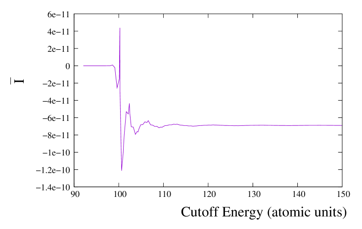
Figure 2: The real part of $\bar{I}$ (see Eq. 52) as a function of the upper cutoff on the intermediate state energy $E_{m}$ in atomic units. We see that the amplitude tends to a significant value as the cutoff goes to infinity.

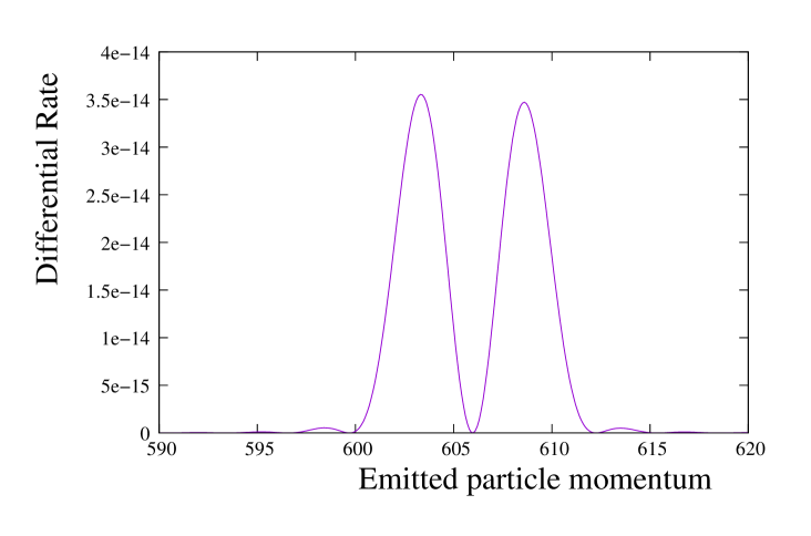
Figure 3: The differential reaction rate $dP/dtdq_{1}$ as a function of the momentum of the emitted particle $q_{1}$, both quantities are in atomic units. Here the value of dimensionless parameter $g^{\prime\prime}$ has been taken to be $10^{-5}$.

5 Conclusions

In this paper we have studied the rate of nuclear fusion at low energies using a $1+1$ dimensional lattice model. The model is a generalization of the standard Kronig-Penney model and incorporates the deep nuclear potential. We consider fusion of a particle, which is analogous to proton, with a lattice site. The fusion rate of the standard first order process is very strongly suppressed due to tunnelling barrier. We consider the rate at second order in perturbation theory. For this case the rate can be large in some special circumstances, as described in earlier papers [18, 19, 20]. In [20] we had considered a three dimensional toy model assuming a step potential. Here we found that the rate was very small if the eigenfunctions show a continuous energy spectrum, which is achieved if the potential vanishes at large distances. However it was argued that in a medium the potential need not be zero at large distances and spectrum is not necessarily continuous. We modelled this phenomenon by assuming an infinite potential barrier beyond a certain distance. This lead to a significant rate for the fusion process [20]. Here we are interested in determining whether a lattice model leads to an observable rate.

The fusion process takes place by emission of two particles, one at each interaction. We have tried a few different models for the interaction. The simplest model in which the interaction Hamiltonian is taken to be of the form given in Eq. 6 with the operator ${\cal O}$ equal to unity we find that the rate is very small. The actual value is difficult to obtain due to a very delicate cancellation among amplitudes due to different intermediate states and we do not pursue this in detail in the present paper. A modified interaction with the operator ${\cal O}$ having a momemtum dependence given in Eq. 50 is found to give a substantial rate. Although many interactions depend on momentum, it is not known whether such an interaction can arise in a real physical situation. We have suggested that it might arise as an effective interaction or a form factor if in the initial stage the process happens through the Hydrogen atom rather than a proton. However, we have not examined this possibility in detail. Nevertheless, our result demonstrates that quantum mechanics does not prohibit a relatively large fusion rate even at very low energies and high potential barrier. To be precise, there does not seem to be any general rule that the amplitude necessarily has to be small exceedingly small even for the second order process.

Our results show that nuclear fusion may take place in a crystalline lattice but requires special conditions. A detailed study is required to determine whether those may be met in a real physical situation. An alternative possibility is presented by a disordered system. In such a system, all states up to a certain energy level are localized. Hence, in a given localized region, relevant for the fusion process, dominant contributions would be obtained only from discretized energy states. Hence we expect that fusion rate be a significant in this case, in analogy with results obtained in [20]. A detailed calculation in a disordered physical system is postponed to future research.

Acknowledgements: We are very grateful to Amit Agarwal for useful discussions.

References

- [1] S. B. Krivit, Development of Low-Energy Nuclear Reaction Research, ch. 41, pp. 479–496. John Wiley & Sons, Ltd, 2011.
- [2] L. I. Urutskoev, Low-Energy Nuclear Reactions: A Three-Stage Historical Perspective, ch. 42, pp. 497–501. John Wiley & Sons, Ltd, 2011.
- [3] M. Srinivasan, G. Miley, and E. Storms, Low-Energy Nuclear Reactions: Transmutations, ch. 43, pp. 503–539. John Wiley & Sons, Ltd, 2011.
- [4] E. Storms, “Introduction to the main experimental findings of the lenr field,” Current Science, vol. 108, pp. 535–539, 02 2015.
- [5] M. C. McKubre, “Cold fusion: comments on the state of scientific proof,” Current Science, pp. 495–498, 2015.
- [6] J.-P. Biberian, “Biological transmutations,” Current Science, vol. 108, pp. 633–635, 02 2015.
- [7] M. Srinivasan and K. Rajeev, “Chapter 13 - transmutations and isotopic shifts in lenr experiments,” in Cold Fusion (J.-P. Biberian, ed.), pp. 233 – 262, Elsevier, 2020.
- [8] T. Mizuno and J. Rothwell, “Excess heat from palladium deposited on nickel,” Journal of Condensed Matter Nuclear Science, vol. 29, pp. 21–33, 2019.
- [9] S. B. Krivit and J. Marwan, “A new look at low-energy nuclear reaction research,” Journal of Environmental Monitoring, vol. 11, no. 10, pp. 1731–1746, 2009.
- [10] K. P. Sinha, “Model of low energy nuclear reactions in a solid matrix with defects,” Current Science, vol. 108, pp. 516–518, 02 2015.
- [11] C. L. Liang, Z. M. Dong, and X. Z. Li, “Selective resonant tunnelling–turning hydrogen-storage material into energetic material,” Current Science, vol. 108, pp. 519–523, 02 2015.
- [12] P. Hagelstein, “Deuterium evolution reaction model and the fleischmann–pons experiment,” Journal of Condensed Matter Nuclear Science, vol. 16, pp. 46–63, 02 2015.
- [13] F. Celani, A. Tommaso, and G. Vassallo, “The zitterbewegung interpretation of quantum mechanics as theoretical framework for ultra-dense deuterium and low energy nuclear reactions,” Journal of Condensed Matter Nuclear Science, vol. 24, pp. 32–41, 02 2017.
- [14] P. Kálmán and T. Keszthelyi, “On low-energy nuclear reactions,” arXiv preprint arXiv:1907.05211, 2019.
- [15] C. Spitaleri, C. Bertulani, L. Fortunato, and A. Vitturi, “The electron screening puzzle and nuclear clustering,” Physics Letters B, vol. 755, pp. 275 – 278, 2016.
- [16] J.-L. Paillet and A. Meulenberg, “On highly relativistic deep electrons,” Journal of Condensed Matter Nuclear Science, vol. 29, pp. 472–492, 02 2019.
- [17] P. Kálmán and T. Keszthelyi, “Forbidden nuclear reactions,” Phys. Rev. C, vol. 99, p. 054620, May 2019.
- [18] P. Jain, A. Kumar, R. Pala, and K. P. Rajeev, “Photon induced low-energy nuclear reactions,” Pramana, vol. 96, no. 96, 2022.
- [19] P. Jain, A. Kumar, K. Ramkumar, R. Pala, and K. P. Rajeev, “Low energy nuclear fusion with two photon emission,” JCMNS, vol. 35, p. 1, 2021.
- [20] K. Ramkumar, H. Kumar, and P. Jain, “A toy model for low energy nuclear fusion,” Pramana, vol. 97, no. 109, 2023.
- [21] E. Merzbacher, Quantum Mechanics. Wiley, 1998.
- [22] J. Sakurai, Advanced Quantum Mechanics. Always learning, Pearson Education, Incorporated, 1967.
- [23] D. D. Clayton, Principles of stellar evolution and nucleosynthesis. The University of Chicago Press, Chicago, 1968.
- [24] N. W. Ashcroft and N. D. Mermin, Solid State Physics. Holt-Saunders, 1976.
- [25] E. Abrahams, 50 Years of Anderson Localization. WORLD SCIENTIFIC, 2010.
- [26] P. A. Lee and T. V. Ramakrishnan, “Disordered electronic systems,” Rev. Mod. Phys., vol. 57, pp. 287–337, Apr 1985.
- [27] J.-P. Biberian, “Anomalous isotopic distribution of silver in a palladium cathode,” Journal of Condensed Matter Nuclear Science, vol. 29, pp. 211–218, 2019.