A Catalogue of Planetary Nebulae Chemical Abundances in the Galactic Bulge

Abstract

In this, the third of a series of papers, we present well determined chemical abundances for 124 Planetary nebulae (PNe) in the Galactic bulge from deep, long-slit FORS2 spectra from the 8.2 m ESO Very Large telescope (VLT). Prior to this work there were only $\sim 240$ bulge PNe with chemical abundances previously determined over a $\sim 50$ year period and of highly variable quality. For 34 of these PNe we are presenting their abundances for the first time which adds $\sim 14$% to the available sample of bulge PNe abundances. The interstellar reddening, physical conditions (electron densities, $n_{\mathrm{e}}$, temperatures, $T_{\mathrm{e}}$), and chemical compositions are derived as single values for each PN but also using different line diagnostics. Selected comparisons with the best literature fluxes for 75 PNe in common reveals that these significant new data are robust, reliable and internally self-consistent forming the largest independent, high quality and well understood derivation of PNe abundances currently available for study.

1 Introduction

Planetary nebulae (PNe) form the most luminous phase in the evolution of low- to intermediate-mass stars with masses ranging from $\sim 0.8$ to $8M_{\odot}$, and luminosity typically falling between $0.5$ and $1.0\times 10^{4}L_{\odot}$. The majority of their luminosity is emitted in a few, very bright emission lines, including several forbidden collisionally-excited lines (CELs) and the hydrogen Balmer series lines. The use of CELs and optical recombination lines (ORLs) allows the accurate measurement of elemental abundances of both light elements like helium and nitrogen, as well as heavier elements such as oxygen, sulphur, and neon in PNe. While helium ORLs are usually the most prominent in nebulae, deeper spectra can also detect ORLs of other heavier elements, making ORLs an alternative to CELs in deriving elemental abundances in PNe. Still, interpreting the results warrants extra caution due to remaining issues with PNe abundance determination, such as the discrepancy between chemical abundances derived from CELs and ORLs (see Peimbert et al., 2017, and references therein), the sulfur anomaly in PNe (a deficit in sulfur abundance, Henry et al., 2004) and the self-enrichment of oxygen in carbon-rich dust PNe (Delgado-Inglada et al., 2015).

As the luminosity of PNe emission lines is typically on the order of $10^{4}L_{\odot}$, they are easily visible across the Galaxy and beyond where individual main sequence stars are too faint. Additionally, PNe provide a detectable population for study close to the crowded Galactic Centre (Durand et al., 1998). PNe are also key representatives of late-stage stellar evolution for low to intermediate-mass stars, where their residual cores end their lives as white dwarfs on the cooling track. The measured abundances of PNe reflect both the results of interior nucleosynthesis (e.g. He, N and C, Chiappini et al., 2003; Henry et al., 2004) in their progenitors and also the interstellar abundances at the time the PN progenitor stars were born from their molecular clouds and enriched with elements only produced in more massive stars (such as sulphur and argon). In these ways, PNe are the best abundance tracers of relatively old stellar populations in our own and external galaxies in the local group, e.g. Arnaboldi (2014).

The Galactic bulge is one key such old stellar population. It contains a large number of PNe, e.g. (Parker et al., 2006) that are of sufficient surface brightness for detailed abundance study. Previously available Bulge PNe abundance determinations have suggested a solar to slightly sub-solar metallicity (Ratag et al., 1992; Chiappini et al., 2009; Pottasch & Bernard-Salas, 2015). On the other hand, spectroscopy of red giants and microlensed main sequence stars in the bulge show a rather wide abundance range. Johnson et al. (2014) report that bulge stars show a range of [Fe/H] between $-0.8$ and 0.4, and $\alpha$ enhancements between 0.0 and 0.3. Uncertainties increase at higher metallicity where molecular blending becomes an issue. Bensby et al. (2013) also report a wide range of bulge metallicities. Chiappini et al. (2009) conclude that oxygen abundances of PNe are 0.3 dex lower than expected for their progenitor bulge stellar population. Due to nucleosynthesis limitations in lower mass stars PNe can only measure [O/H] rather than [Fe/H], but Smith et al. (2014) and Smith et al. (2017) determined zinc abundances (expected to mirror Fe) for a small sample and confirm the tendency towards solar abundances. The observed differences between observed stellar and PNe abundances in the bulge remains problematic and impacts the question of the origin of the bulge, as either a pseudobulge, arising from scattered disk stars, or an old classical bulge. Hence, getting a better handle on a wider sample of Bulge PNe abundances could have significant implications and was a major motivation for this work.

In this study, we assume that chemical abundances determined for any individual PN are representative of the entire nebula. We recognise that internal abundance variations may exist, albeit likely modest, e.g., Manchado et al. (1988); Danehkar et al. (2013); Mari et al. (2023). For most extant literature, and for all comparisons made in this study, each PNe produces a single, overall abundance estimate determined from an integrated 1-D spectrum across the spectrograph slit. We know PNe are complex, structured and resolved 3-D sources with ionisation stratification, internal condensations, and other features. Factors such as spectrograph slit widths and positions, in terms of orientation and offsets from any central star, can vary between different works and finally that observing conditions (seeing, transparency, airmass and etc.) also differ. Hence, different literature compilations may not sample exactly the same part of a given PN. Integral Field Unit (IFU) work, such as Danehkar et al. (2013) and García-Rojas et al. (2022), can cover entire PNe, or at least representative fractions of the full projected form, to create 3-D spectroscopic data cubes. Existing IFU PNe studies have already demonstrated that physical conditions and chemical abundances can vary across a given PN, and these variations do not usually correspond directly to those observed in line fluxes. Instead, the final physical conditions derived from observations with different slit positions predominantly reflect the results in regions covered by the slit where the line fluxes are strong, potentially leading to discrepancies in results. Until direct point-to-point mapping of physical parameters and chemical abundances based on IFU observations are available for large samples of PNe from different studies, this type of research remains essential. Furthermore all PNe in this study are compact ($\leq$10 arcseconds across) so a decent, central fraction of each PN is always sampled.

2 The formation of the Galactic Bulge

To help understand the context of abundances determined for a significant sample of bulge PNe, a brief introduction to current understanding of the formation of the Galactic bulge is provided. There are currently two main scenarios (e.g. Raha et al., 1991; Debattista et al., 2004; Brooks & Christensen, 2016; Fisher & Drory, 2016). The classical scenario involves the gravitational collapse of primordial gas and/or the hierarchical merger of sub-clumps, leading to rapid star formation and disk accretion. This type of bulge is dominated by an old, metal-rich, spheroidal population characterised by an enhancement of $\alpha$-elements (e.g. Wyse et al., 1997; Zoccali et al., 2008; Bensby et al., 2011a; Johnson et al., 2011). Alternatively, the secular evolution of the disk, driven by non-axisymmetric structures such as bars, can slowly bring gas to the centre, turning it into a spheroid via the buckling instability or resonant thickening event, forming a so-called "pseudobulge" (Combes & Sanders, 1981; Combes & Elmegreen, 1993; Athanassoula, 2005; Sellwood, 2014, for a review).

Pseudobulges form at a slower rate, with longer star formation timescales and have younger stellar populations than classical bulges (e.g. Feltzing & Gilmore, 1999; Loon et al., 2003; Kormendy & Kennicutt Jr, 2004, and references therein). The bulge’s vertical metallicity gradient was initially interpreted as due to dissipative collapse during the formation of a classical bulge. However, recent kinematic constraints suggest the bulge could have a composite nature, with a substantial fraction of pseudobulge, or it might purely be a pseudobulge (Shen et al., 2010; Di Matteo et al., 2014). Further evidence for a pseudobulge comes from the kinematic and chemical properties of the bulge stellar populations which show a concordance with the stellar populations identified in the inner disk of the Galaxy (Babusiaux et al., 2010; Gonzalez et al., 2011; Bensby et al., 2011b; Uttenthaler et al., 2012).

The metallicity distribution functions (MDF) obtained from red giant branch (RGB), red clump (RC) and M giant stars in different bulge regions exhibit similar peaky structures (see Fig. 4 in Barbuy et al. (2018)). Ness et al. (2013) observed three predominant MDF peaks derived from 28,000 ARGOS bulge stars (Freeman et al., 2013). These are associated respectively with the pseudobulge, the vertically thicker pseudobulge, and the inner thick disc, indicating a predominant pseudobulge fraction. Numerical simulations in Martinez-Valpuesta & Gerhard (2013) suggest that bar and buckling instabilities could produce vertical and longitudinal metallicity gradients. This is supported by observational evidence from the photometric metallicity map of RGB stars in Gonzalez et al. (2013).

Bensby et al. (2017) performed an age analysis of 90 microlensed dwarf stars to investigate the evolutionary history of the bulge. The results indicate a considerable fraction of young stars (26% of the sample are younger than 5 Gyr), leaving limited room for a classical bulge. However, the sample size is modest, and observations of stars could be biased towards metal-rich components or mixed with foreground objects. Therefore, an independent line of detailed abundance measurement evidence from carefully selected bulge PNe could be crucial to inform this debate. The accurate determination of bulge PNe membership can be achieved through a range of powerful selection criteria, as outlined by Rees & Zijlstra (2013) and utilized in this study (detailed in Paper I). These criteria include:

1. the PN’s location within the inner 10^∘ of the Galactic Centre,

2. a measured angular size greater than 2 arcseconds but less than 35 arcseconds; see Acker et al. (2006),

3. availability of the PN’s radio flux at $5\ \mathrm{GHz}$ in the range of 4.2 mJy to 59.1 mJy (Acker et al., 1992; Siódmiak & Tylenda, 2001).

These criteria effectively exclude foreground contamination, as demonstrated by Stasinska & Tylenda (1994) and Rees (2011). Indeed, our independent evaluation of potential foreground contamination determined by examining HASH PNe in two zones either side of the Bulge in Galactic longitude that satisfy our Bulge selection criteria, indicate we might expect up to 15% contamination. In a previous study using a limited sample of bulge PNe, Escudero & Costa (2001) found a possible vertical abundance gradient that suggested a few PNe with low N/O ratios could have originated from old, lower mass progenitors. Later, an attempt at PNe age determination was made for 31 objects in Gesicki et al. (2014) based on central-star masses derived from photo-ionization modelling. Even though this is a small sample, a similar fraction of young stars to dwarf stars was found. Chemical abundances used in both studies are sub-samples of data provided by Chiappini et al. (2009).

However, to make real progress, determination of accurate chemical abundances for a larger sample of bulge PNe is needed and as derived from deep and high signal-to-noise ratio (s/n) spectra. Such an enlarged sample can better characterize the nature of underlying stellar populations of both PNe and stars, and so help us understand the chemical evolution in the bulge.

In this, the third in a series of papers that present different sets of results for 136 compact, confirmed PNe within a $10\times 10$ degree region of the Galactic bulge, we report our detailed abundance determinations. Our in depth analysis of these results are provided in Paper IV, Tan et al., in preparation. The abundances reported here derive from deep, medium-resolution spectroscopy from our VLT/FOSR2 observations from a very careful and homogeneous data reduction. The forensic selection of this well-defined sample and the evaluation of the associated PN imaging data and underlying morphology were discussed in Paper I (Tan et al., 2023a) while in Paper II we present results of a remarkable 5$\sigma$ PN major axis alignment signal but only for a special subset of the bulge PNe sample that host short period binaries (Tan et al., 2023b).

Sec. 3 describes the observations and data reduction. The excellent consistency and quality of our data shown in Sec. 4 and 5 is demonstrated through reliable previous literature studies of 75 objects in common with our sample. The derived plasma diagnostics and elemental abundances for the sample are given in Sec. 6. We present an in-depth discussion in Sec. 7 and our summary and conclusions in Sec. 8.

3 Observations

3.1 Long-slit spectroscopy with the VLT/FORS2

The long-slit spectroscopic observations used in this study were conducted with the FORS2 instrument on the 8 m ESO VLT/UT1 (Appenzeller et al., 1998) between April 2015 and July 2018 under program IDs 095.D-0270(A), 097.D- 0024(A), 099.D-0163(A), and 0101.D-0192(A) with PI Rees and co-Is Zijlstra and Parker. Although the observations were conducted as ‘filler’ programs, where observations could be performed under any conditions (e.g. poor seeing, low transparency due to clouds and/or high humidity) a decent fraction are of very high quality. The observed sample of 138 PNe are between 2 to 10 arcsec in angular size and fall within the inner 10 degrees of the Galactic Centre. All are considered bulge members based on criteria in Zijlstra (1990) and Rees & Zijlstra (2013). Among the nearly 4000 currently confirmed Galactic PNe contained in the “Gold Standard” HASH database,(e.g. Parker et al., 2016; Parker, 2022), the objects PNG 005.9-02.6 and PNG 007.5+04.3 from the original program target selection are now classified as symbiotic stars due to their mid-infrared images and spectroscopic features. These are now excluded from this study, thus leaving 136 PNe.

Table 1 provides a summary of the observing dates, exposure times, and the number of objects covered in each VLT program. Unfortunately, for 12 high surface brightness objects observed, several bright but important emission lines for standard abundance determinations were saturated even in the shortest exposures, and no line flux measurements were available in the literature. Consequently, we excluded these nebulae from further analysis in our study.

Table 1: Summary of the VLT observing programs.

Program ID	Obs. Date	# of PNe	Amount of Time
		Observed	[nights]	[hours]
095.D-0270(A)	Apr - Aug 2015	62	25	74
097.D-0024(A)	May - Sep 2016	42	23	54
099.D-0163(A)	Jun - Sep 2017	16	9	19
101.D-0192(A)	May - Jul 2018	23	11	31
Total:		138∗	68	178

• * The observations of faint PNe PNG 005.8-06.1, PNG 007.5+04.3, PNG 355.9-04.2, PNG 357.3+04.0 and PNG 358.9+03.4 were repeated due to either observing conditions or issues with the slit position.

To date, approximately 240 bulge PNe have had their chemical abundances determined. Our study provides new abundance data for 34 PNe that were previously unreported, effectively increasing the available sample of bulge PNe for study by 14%. Additionally, 25% of the existing literature results are considered highly unreliable due to an uncertainty greater than 0.3 dex. Our work has achieved an abundance precision typically better than 0.3 dex including for 6 PNe in common with the poorly determined examples.

3.2 Spectroscopic instrumental configuration

The VLT spectroscopic detector was a mosaic of two $2\text{k}\times 4\text{k}$ MIT/LL CCDs with $2\times 2$ on-chip binning (resulting in 0.25 arcsec/pixel). The instrument was used in Long Slit Spectroscopy (LSS) mode with a slit measuring $0.5^{\mathrm{"}}\times 6.8^{\mathrm{{}^{\prime}}}$ on the sky. Two grisms, GRIS1200B+97 (G1200B) and GRIS600RI+19 (G600RI) were employed to provide low–medium resolution optical spectroscopy.The G1200B grism covers the blue spectral range from $~{}3360$-$5110$ Å  with a medium spectral resolution up to 1420, while the G600RI grism, used with GG435 blocking filter, covers the red spectral range from $\sim$5120-8450 Å  with a lower resolution up to 1000. As limited by the colour range of standard stars used for flux calibration, the combined wavelength coverage of the spectra was $3700$-$8450$ Å  for 46 PNe and $3750$-$8450$ Å  for 90 PNe due to small differences in instrumental set-up over the 3 year period of the VLT observing program. Exposure times varied from 2 to to 1500 seconds. Each PNe target had two exposures with the blue and red grisms respectively typically of 30s and 1000s to be sensitive to very bright and faint emission lines and in order to avoid both saturation or no line detection depending on the surface brightness of the PNe.

3.3 Data reduction

The two-dimensional long-slit spectra were reduced with a typical multi-step method. First, cosmic rays were removed using a Python implementation of the L.A.Cosmic algorithm (Van Dokkum, 2001). A standard reduction procedure including bias subtraction and wavelength calibration was then carried out using the ESO pipeline with a Reflex workflow (Freudling et al., 2013). As the bright skylines, e.g. [O i] $\lambda\lambda$5577, 6300 and 6363, become strongly inhomogeneous in the spatial direction in longer wavelength exposures, a careful sky subtraction was performed. This was via spline fitting to lines in carefully-chosen sky windows below and above the object spectra using a figaro routine (Shortridge et al., 2014) in starlink (Warren-Smith et al., 2014). In addition, as the Galactic bulge has a dense stellar population, the spectra are almost always contaminated by other stars that fall within the width and along the length of the slit. Such contaminating sources and any PN central star continuum emissions were carefully removed where practical with the iraf.continuum routine. The sky-subtracted, continuum-removed spectra were then corrected for atmospheric extinction and flux-calibrated using the ESO pipeline.

The flat field lamp used for the GRIS1200B grism has a documented instability in its spectral energy distribution (SED), which could introduce wavelength-dependent variations across the blue spectra. We decided not to perform an SED normalization on the response curve for the blue spectra (-use_flat_sed = false) to avoid substantial systematic distortions in calibrated fluxes even though this is the default pipeline option. This approach is in line with the FORS2 manual’s recommendation. By comparing our reductions with and without SED normalization, we found that this issue can lead to overestimated blue emission line fluxes, particularly for those with wavelengths in the central region of the blue spectral coverage important for abundance determination, such as H$\gamma$ and [O iii] $\lambda$4363. This overestimation could amount to up to 20% with a moderate wavelength dependence that could results in a median decrease of 160 K in $T_{\mathrm{e}}$([O iii]).

To maximise the signal-to-noise, especially for weaker lines, a 2-D frame pixel was attributed to an emission line only when it and at least half of its neighbouring pixels are brighter than 2$\sigma$ of the background noise. Remaining pixels were considered part of the background and set to zero. This is following a similar methodology used by Górny et al. (2009). The final, reduced, extracted 1-D spectra were obtained after summing the frame perpendicular to the dispersion direction. The mean systematic errors associated with the wavelength calibration and flux calibration propagated through the pipeline are $\sim$2%.

For more than 85% of the PNe in our sample we detected over 60 different emission lines from their long exposure spectra. All emission lines fluxes were then measured from the extracted 1-D spectra using the automated line fitting algorithm (alfa; Wesson, 2016). The reliability of alfa for measuring PNe line fluxes has been demonstrated in previous studies (e.g. Sowicka et al., 2017; Boffin et al., 2018). alfa performs Gaussian fits to input spectrum and drives the final line fluxes by constructing and optimising a synthetic spectrum with a generic algorithm. The genetic parameters were tested with grids of values and the configuration that gives the smallest combined residuals was employed. Errors in emission line fluxes were estimated from the RMS values of residuals after subtracting the fitted spectrum. Flux measurement for some PNe emission lines with alfa can be unreliable due to ineffective deblending of the [N ii] $\lambda$6548 and H$\alpha$ lines in low-excitation nebulae at these modest spectral resolutions. Here the [N ii] emission is much weaker than H$\alpha$. To address this we first measured the [N ii] $\lambda$6583/$\lambda$6548 flux ratios and compared them with their theoretical value of 3.05 (Storey & Zeippen, 2000) to identify spectra that were affected. In these cases, careful manual measurements of [N ii] $\lambda$6548, H$\alpha$ and [N ii] $\lambda$6583 line fluxes were carried out using the iraf.splot deblending tool.

The typical uncertainty in our line flux measurement is $\sim$7%. For some fainter emission lines and the [N ii] $\lambda$6458 line, which can suffer from strong blending with H$\alpha$, the uncertainties in line flux measurements could be up to 30%. Fortunately, multiple exposures of the same PNe are often available, albeit with different exposure times. This facilitates cross-checking of line fluxes measured from different spectra and allows identification of cases where cosmic-rays impinge on an emission line during a particular exposure. Fluxes of all main hydrogen Balmer lines, including H$\alpha$, H$\beta$, H$\gamma$, and H$\delta$, and the ratios of common forbidden line doublets, e.g. [O ii] $\lambda\lambda$3726,29, [S ii] $\lambda\lambda$6716,31 and [O ii] $\lambda\lambda$7319,30 were assessed using iraf.splot. Manual verification was employed when necessary to eliminate any inaccurately identified lines or faint central star attributes in some PNe spectra.

In cases where multiple spectra were taken, the longest exposures, typically of 1000 seconds, were used because of their higher s/n and detection of weaker lines. Here some strong emission lines can be saturated such as [O iii] $\lambda$5007 and H$\beta$ in the blue arm and [N ii] $\lambda$6583 and H$\alpha$ in the red arm. The [O iii] $\lambda$5007 and [N ii] $\lambda$6583 saturated lines can usually be scaled using the weaker component if unsaturated in combination with the theoretically predicted line ratios or by using the shorter exposure measurements. A scaling factor was estimated using other bright, unsaturated lines in the same arm. This correction method is highly effective with associated uncertainties usually less than 2%. For a few objects where the brightest emission lines are saturated in both the long and shorter exposures, literature line ratios for the same PNe were used for the correction, provided that the emission line flux ratios (e.g. [N ii] $\lambda\lambda$6548,83, [He i] $\lambda\lambda$5875,6678, [S ii] $\lambda\lambda$6716,31) agree within the uncertainty estimates.

Fig. 1(a) and 1(b) display the [O iii] $\lambda$5007/$\lambda$4959 and [N ii] $\lambda$6583/$\lambda$6548 flux ratios obtained from the unsaturated spectra, which were used to assess uncertainties associated with the data reduction. We corrected for the effects of interstellar extinction by using the hydrogen Balmer ratio (see Sec.3.5 for details), since observed line ratios would be slightly higher than theoretical values. The combined 7% uncertainty interval estimated from the individual 2% data reduction uncertainties of the two sets of emission lines is also presented. Our results showed that the determined [O iii] line ratios agree with the theoretical value within the uncertainties, without any systematic bias as a function of line flux. This provides a base level confidence in both the quality of our data reduction process and spectra. Similarly, the [N ii] ratios did not exhibit any significant bias, except for one outlier where a larger deviation of the line intensity ratio was observed. This deviation was due to a very weak [N ii] emission in comparison to H$\alpha$ (F$($H$\alpha)/$F([N ii] $\lambda 6583)>~{}25$) in this particular PN, and the associated uncertainties.

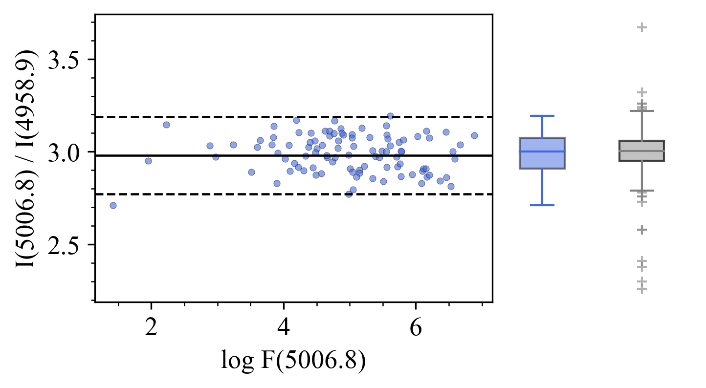
(a) [O iii] line ratios for 100 PNe from our sample

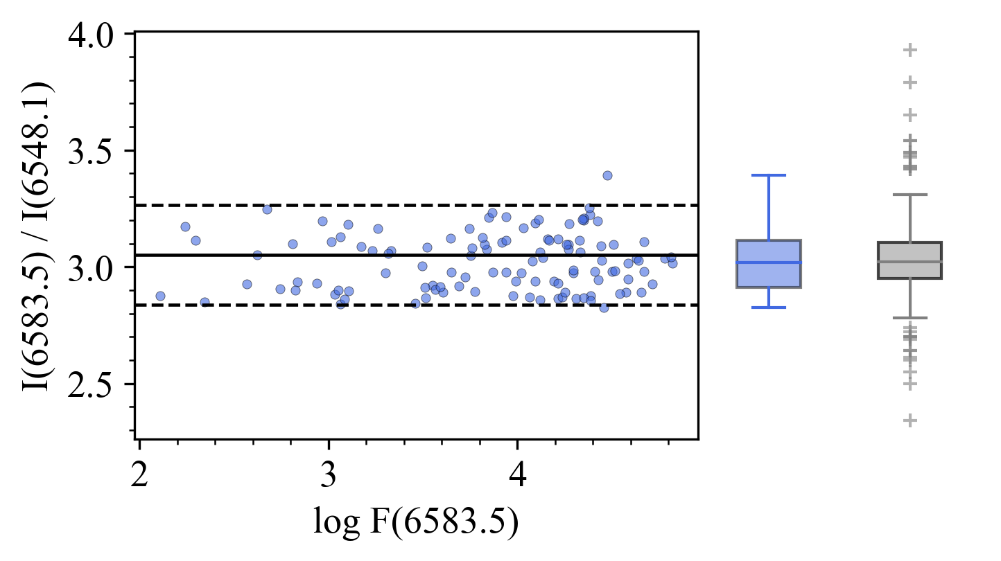
(b) [N ii] line ratios for 114 PNe from our sample

Figure 1: Comparison of measured flux ratios of [O iii] and [N ii] forbidden emission lines from our observations with their theoretical values. The left panels shows de-reddened line ratios plotted against the [O iii] $\lambda$5007 or [N ii $\lambda$6584 flux in $10^{-16}\mathrm{erg~{}cm^{-2}s^{-1}}$ on a log scale, with saturated spectra excluded. The black solid line represents the theoretical line ratio value of 2.98 and 3.05, respectively, while the dashed lines indicate a 7% deviation corresponding to the combined typical uncertainty in the data reduction and spectrum fitting. The right panels shows box plots that compare our results (blue) with those for 124 Galactic PNe from Rodríguez (2020) (grey). The boxes depict the 25th to 75th percentiles, with the median indicated by a horizontal line. The whiskers extend to the 10th and 90th percentile, while outliers are represented by individual crosses. The results show excellent agreement to within the anticipated 7% errors and no bias as a function of flux, providing a solid base level confidence in the reliability of the data reduction.

Relative line intensities were used to determine chemical abundances in this work without the need for absolute fluxes. Measured line fluxes were scaled to I$\mathrm{\left(H\beta\right)}=100$, which is a common practice. Complete line intensity lists of emission used for this abundance analysis for each PNe in our sample are available in online supplementary materials.

3.4 Examples of reduced ESO 8 m VLT 1-D PNe spectra

Fig. 2 shows fully reduced blue and red arm ESO 8 m VLT 1-D spectra for three example PNe from our sample; PNG 005.5+06.1, PNG 359.8+06.9, and PNG 000.9-04.8. These are selected to represent PNe with low, medium, and high excitation characteristics and feature a typical range of emission lines under those conditions. The figure shows at left the narrow-band acquisition image for each PNe together with the relative placement of the spectrograph slit and then the resultant 1-D spectrum to the right. Key emission lines are identified.

For PNG 005.5+06.1, Acker et al. (1991) reported the only spectroscopic observations previously available and as obtained with the ESO 1.52 m telescope. They detected 16 emission lines but no lines from ions of Ne and Cl. Our much higher s/n VLT spectra detected 66 emission lines, including [Ne iii] and [Cl iii] lines, thus enabling the determination of Ne and Cl abundances for the first time. The best available spectra of PNG 359.8+06.9 was reported in Escudero et al. (2004) and was also observed with 1.52 m ESO telescope, detecting 29 emission lines. Our VLT spectra revealed 56 emission lines, notably detecting [S ii] $\lambda$4069 and [Cl iii] $\lambda\lambda$5517,37 lines, which also allowed proper determination of [S ii] temperature and [Cl iii] density estimates. The best previously available spectra of PNG 000.9-04.8 are those presented in Górny et al. (2009) from the CTIO 4 m telescope that provided 25 CELs and ORLs of hydrogen and helium. Our VLT spectra detected 87 lines, providing better spectral coverage and importantly, detecting recombination lines of heavier elements for this object for the first time.

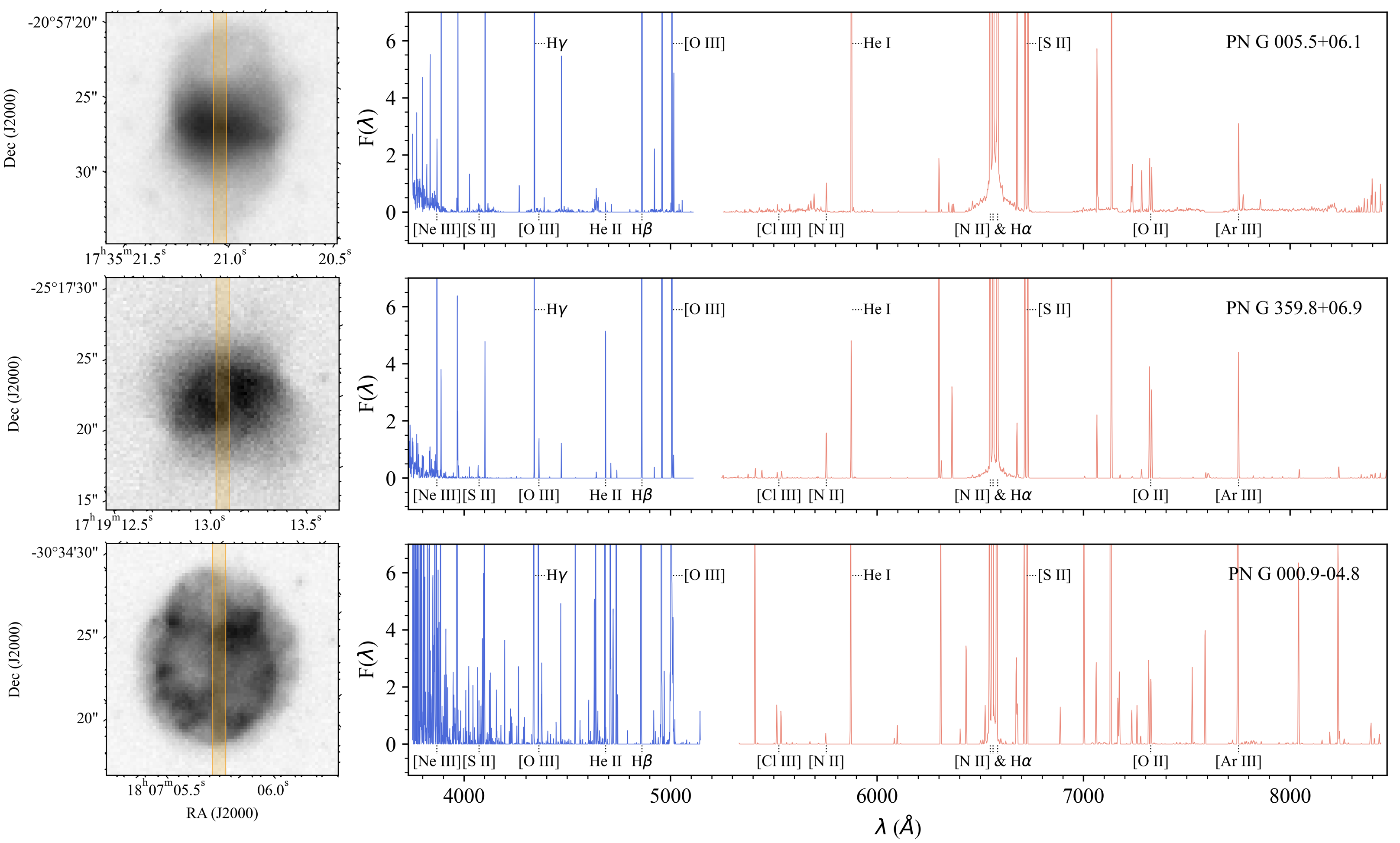
Figure 2: Illustrative examples of optical VLT/FORS2 spectra of three PNe with different degrees of excitation. The upper panel displays the observations of a low excitation PN, PNG 005.5+06.1, with an acquisition image on the left and a reduced 1-D spectrum on the right. The PN image presented is 18 arcsec on a side and the slit position and width is indicated by the orange shaded region. The spectroscopic observations from the blue and red arms are distinguished using blue and red colours. The fluxes are given in units of $10^{-16}\mathrm{erg~{}cm^{-2}s^{-1}}$. Some selected nebulae emission lines are also identified. The middle and lower panels display the observations of medium and high excitation objects, PNG 359.8+06.9 and PNG 000.9-04.8, respectively with the same display scheme.

3.5 Chemical abundance determination using neat

The physical conditions and chemical abundances for the PNe sample (refer Sec. 6) were determined iteratively using the Nebular Empirical Analysis Tool (neat, version 2.3.46; Wesson et al., 2012). The robustness of neat in deriving abundances with the VLT/FORS2 spectroscopy has been demonstrated in previous works, e.g. Jones et al. (2016) and Wesson et al. (2018). The chemical abundance determination process adopted in neat is described below.

3.5.1 Extinction correction

Prior to further work, a correction for the extinction due to absorption and scattering of light by interstellar dust grains was applied using the Fitzpatrick (1999) curve and H$\beta$, H$\gamma$, H$\delta$ lines. The logarithmic extinction at H$\beta$ (extinction coefficient), c(H$\beta$), in neat, is computed by comparing the observed H$\beta$/H$\gamma$ and H$\gamma$/H$\delta$ line ratios with their intrinsic values, assuming an electron temperature, $T_{\mathrm{e}}$, of 10,000 K and an electron density, $n_{\mathrm{e}}$, of 1000 $\mathrm{cm^{-3}}$, as commonly employed. Afterwards, the line intensities were de-reddened, and the electron temperatures and densities were actually determined as outlined later. The updated $T_{\mathrm{e}}$ and $n_{\mathrm{e}}$ values were then used to recalculate the intrinsic Balmer line ratios, and the line intensities were de-reddened using the revised c(H$\beta$) value. These steps are repeated until the values converge.

As the blue and red spectra from the two spectrograph arms are non-overlapping, the H$\alpha$ line was used to scale the red spectrum such that the H$\alpha$/H$\beta$ ratio yield an extinction coefficient consistent with the estimate from the blue spectrum. This scaling factor comes from possible slight changes in either slit position or seeing conditions when taking multiple exposures of the same object and reacquiring blue or red spectra. Typically, our derived scale factor values are within $\pm$20% of unity. Rarely, slightly larger or smaller factors arise from larger shifts in slit coverage or larger variations in observing conditions. This is usually for cases where there was a few months between repeat observations of the same PN. Our [N ii] line ratios agree very well with theoretical values (see in Fig. 1(b)), demonstrating the accuracy of both the [N ii] and H$\alpha$ line flux measurements. The s/n ratio of the hydrogen Balmer lines used for this purpose are generally $>100$, so the uncertainty caused by such scaling is small.

3.5.2 Physical conditions

In neat, a three-zone ionization scheme was implemented to categorise emission lines based on their ionization potential (IP): those with IP $<20$ eV are designated as the low ionization zone, those with 20 eV $<$ IP $<$ 45 eV are classified as the medium ionization zone, and lines with IP $>45$ eV are assigned to the high ionization zone. Table 2 presents the representative values of $T_{\mathrm{e}}$ and $n_{\mathrm{e}}$ for each zone (e.g. Osterbrock & Ferland, 2006). The electron density measurements from the two main sets of different diagnostic lines used here are given equal weight. In determining $T_{\mathrm{e}}$, the [N ii] diagnostic is given a dominant weight for the low-ionization zone due to its lower dependence on electron densities compared to other diagnostic lines (Méndez-Delgado et al., 2023), while [O iii] is prioritised for the medium-ionisation zone because of the higher brightness of the lines and the broader sensitivity range they offer (Proxauf et al., 2014). neat also uses other temperature and density diagnostics from other ionic species in the different ionisation zones used as shown in Table 2 and these are all given equal weight.

Table 2: Plasma diagnostics used for the low, medium and high ionisation zone as applied by neat.

Zone	Temperature diagnostics	Density diagnostics
Low	[N ii] $\frac{\lambda\lambda 6548+84}{\lambda 5755}$	[O ii] $\lambda$3726/$\lambda$3729
	[O ii] $\frac{\lambda\lambda 7319+30}{\lambda\lambda 3726+29}$	[S ii] $\lambda$6716/$\lambda$6731
	[S ii] $\frac{\lambda\lambda 6716+31}{\lambda\lambda 4068+76}$
Medium	[O iii]$\frac{\lambda 4959+\lambda 5007}{\lambda 4363}$	[Cl iii$]\lambda 5517/\lambda 5537$
	[Ar iii] $\frac{\lambda\lambda 7135+7751}{\lambda 5192}$	[Ar iv$]\lambda 4711/\lambda 4740$
High	[Ar v] $\frac{\lambda 6435+\lambda 7005}{\lambda 4625}$	-

neat primarily uses atomic data obtained from the chianti 9.0 database (Dere et al., 1997, 2019) for CELs, except for O⁺ and S²⁺, which have documented errors in chianti data, Kisielius et al. (2009); Wesson et al. (2012). The transition probabilities and collision strengths of O⁺ were adopted respectively from Zeippen (1982) and Pradhan (1976). For S²⁺, the transition probabilities from Mendoza & Zeippen (1982) and collision strengths from Mendoza & Zeippen (1983) were used. The atomic data for recombination lines (ORLs) in neat are from multiple sources, with details available in Table 1 of Wesson et al. (2012). neat derived the uncertainties in electron temperatures and densities through a Monte Carlo approach with 10,000 realisations.

Recombination excitation contributes to the total observed intensities of the [N ii] $\lambda$5755, the [O ii] $\lambda\lambda$7319,30 and the [O iii] $\lambda$4363 auroral lines. These were corrected in neat according to equations (1-3) in Liu et al. (2000). The recombination contribution to [N ii] and [O ii] lines could be significant as most nitrogen and oxygen are in the form of N²⁺ and O²⁺. As a result, such corrections may lead to a decrease in $T_{\mathrm{e}}$([N ii]) by up to 20% as well as a change in O⁺ ionic abundance by up to 0.3 dex according to (Rodríguez, 2020). Ignoring these corrections, as in earlier studies with low s/r spectra, could impact the accuracy of abundances results as the O⁺ ionic abundance is key in the ICF formula for most elements. We employed the physical parameters obtained from CELs to calculate the ionic abundances from recombination lines used in equations (1-3) in Liu et al. (2000). However, according to studies such as Liu (2006) and Yuan et al. (2011), ORLs might originate from cooler regions within the nebulae. In some cases of extremely high abundance discrepancies, for example, in Liu et al. (2006) albeit with large uncertainties, the electron temperature derived from the hydrogen Balmer jump ($\lambda<3645$Å) for Hf 2-2 is as low as $\sim 1000$ K. Similarly, García-Rojas et al. (2022) estimates electron temperatures in ORL emission regions for three objects to be around 4000K, based on a comparison of 2-D temperature maps derived from [N ii] and [S iii] lines. Unfortunately, such methods for electron temperature determination could not be performed with our observations.

For the [N ii] $\lambda$5755 emission line, we detected at least one of the N ii lines from multiplet V3 and 3d-4f transitions in more than half of PNe with the VLT/FORS2, along with other multiplets such as V12 and V20, as well as singlets V5 and V28 in our deeper spectra. Since stronger V3 and 3d-4f lines were better detected, we used the flux-weighted N²⁺ ionic abundances derived from them for the [N ii] $\lambda$5755 recombination correction. When either the ORL contribution to [N ii] $\lambda$5755 estimated from V3 or 3d-4f transitions exceeds the observed intensity, the other is used. Through a detailed analysis, Rodríguez (2020) demonstrated that ORLs have a minimal contribution to [N ii] $\lambda$5755 intensities for objects with low degrees of ionization ($\log(\text{O}^{2+}/\text{O}^{+})<1$). Therefore, for objects with an with a estimated contribution of ORLs leading to a decrease greater than 10% in $T_{\mathrm{e}}$, we do not apply these corrections if the He²⁺ emission lines are reliably observed in our spectra and the resulting $\log(\text{O}^{2+}/\text{O}^{+})<1.4$. This is because the observed ORLs may be significantly contaminated by continuum fluorescence excitation (Escalante & Morisset, 2005; Escalante et al., 2012). We derived the recombination O⁺ abundance using the V1, V2 and V10 multiplets.

3.5.3 Chemical abundances

Ionic abundances were first determined from the de-reddened collisionally excited line intensities listed in Table.3. The total elemental abundances (Sec. 6) were obtained by multiplying the sum of ionic abundances with the corresponding ionization correction factors (ICFs) to account for the contribution of unobserved ions. In our case, we adopt the ICF scheme derived in Delgado-Inglada et al. (2014), hereafter DMS14, for all elements, except for N, for which we used the classical N/O $=$ N⁺/O⁺ relation in Kingsburgh & Barlow (1994) (KB94), following the recommendations of Delgado-Inglada et al. (2015).

Table 3: The list of collisional excitation lines used for the ionic abundance determinations in this work.

$\mathrm{X}^{\mathrm{i}+}$	Line
$\mathrm{He}^{+}$	${\mathrm{He}}$ i $\lambda\lambda 4471,5876,6678$
$\mathrm{He}^{2+}$	${\mathrm{He}}$ ii$~{}\lambda\lambda 4686,5412$
$\mathrm{N}^{+}$	$[\mathrm{N}$ ii$]~{}\lambda\lambda 5755,6548,6584$
$\mathrm{O}^{+}$	$[\mathrm{O}$ ii$]~{}\lambda\lambda 3726,3729,7319,7330$
$\mathrm{O}^{2+}$	$[\mathrm{O}$ iii$]~{}\lambda 4959,5007$
$\mathrm{Ne}^{2+}$	$[\mathrm{Ne}$ iii$]~{}\lambda 3868$
$\mathrm{S}^{+}$	$[\mathrm{S}$ ii$]~{}\lambda\lambda 6716,6731$
$\mathrm{S}^{2+}$	$[\mathrm{S}$ iii$]~{}\lambda 6312$
$\mathrm{Cl}^{2+}$	$[\mathrm{Cl}$ iii$]~{}\lambda\lambda 5517,5537$
$\mathrm{Cl}^{3+}$	$[\mathrm{Cl}$ iv]$~{}\lambda 7531,8046$
$\mathrm{Ar}^{2+}$	$[\mathrm{Ar}$ iii$]~{}\lambda\lambda 7135,7751$
$\mathrm{Ar}^{3+}$	$[\mathrm{Ar}$ iv$]~{}\lambda\lambda 4711,4740$
$\mathrm{Ar}^{4+}$	$[\mathrm{Ar}$ v$]~{}\lambda\lambda 6435,7005$

4 Evaluation of Data Quality

To ensure the internal consistency and quality of our data, we compared chemical abundances and physical parameters derived from both the long and shorter exposure spectra of the same PNe, as well as estimates of ionic abundances obtained using different emission lines of the same ionic species. This internal comparison is crucial in assessing the quality of our spectra and the reliability of measurements and estimations derived from them. This is followed in Sec. 5 with an external comparison with literature values. Chemical abundances are expressed on a logarithmic scale, where $\log\mathrm{(H)}=12$.

4.1 Comparison of results from the short and long exposures

Our observations include short-exposure spectra in both blue and red arms for 80 PNe. As the observation configurations show minimal variation, the chemical abundances derived from these spectra are expected to be consistent with their long-exposure counterparts due to the same amount of interstellar extinction and the emission from the same object region passing through the slit. However, background noise, stellar continuum variations, or low-level instrumental variabilities could result in small discrepancies. Here, we compare the chemical abundances independently derived from short and long exposures of the same PNe to assess the consistency of the results under different s/n levels of spectroscopic observations.

4.1.1 Extinction coefficients

The short exposure spectra of three PNe in our sample, PNG 000.1+02.6, PNG 000.3+06.9 and PNG 359.8+05.2, did not yield a detection of H$\gamma$. Additionally, the short exposure spectra of 4 objects PNG 356.5-03.6, PNG 357.1+04.4, PNG 357.9-03.8 and PNG 358.5+02.9 had low s/n for H$\gamma$ which prevented accurate measurements. This caused a severe overestimation of their extinction coefficients and so we were unable to derive chemical abundances for these combined seven PNe using the short exposures to compare with their well-determined longer exposure counterparts. These PNe were excluded from our comparison.

The extinction coefficient, c(H$\beta$), estimated from the short and long exposures are in good agreement, with a median difference of $-0.07$. Minor discrepancies can also arise due to slight changes of theoretical hydrogen Balmer line ratios with different physical parameters. For example, in the low-density limit, increasing the electron temperature from 5,000 K to 10,000 K could result in a shift of 3% in H$\beta$/H$\gamma$ ratio (see Table 4.2 in Osterbrock & Ferland, 2006).

4.1.2 Nebular plasma diagnostics

The nebula physical parameters for our PNe, including electron densities and temperatures, determined from the shorter exposure spectra generally exhibit good agreement with their longer exposure counterparts, with no systematic differences and with discrepancies typically well below 0.1 dex. However, due to the lower detection levels of weaker plasma diagnostic lines in the shorter exposure spectra, the discrepancy for individual PNe can exceed 0.5 dex.

A comparison of the electron temperature estimates from the two commonly used diagnostics, $T_{\mathrm{e}}$([N ii]) and $T_{\mathrm{e}}$([O iii]), obtained from the short and long exposures, shows a generally good agreement. The median differences are $0.004\pm 0.03$ and $-0.01_{-0.10}^{+0.01}$ dex, respectively, with errors originating from the 16th and 84th percentile values. For the other two temperature diagnostics with larger spectral separations, [O ii] and [S ii], larger deviations were observed, with median differences of $-0.06_{-0.7}^{+0.08}$ and $-0.06_{-0.12}^{+0.08}$ dex, respectively. This can be attributed to varying estimates of extinction corrections as pointed in Sec.4.1.1. The median differences in resulting electron temperatures adopted for the low- and medium-ionization zones, when comparing short exposures to long exposures, are $0.002_{-0.06}^{+0.04}$ and $-0.01_{-0.08}^{+0.03}$ dex, respectively.

We noticed a systematically lower $T_{\mathrm{e}}$([O iii]) estimates from the short-exposures spectra. Fig. 3 illustrates the difference in $T_{\mathrm{e}}$([O iii]) obtained from the short and long exposures as a function of F($\lambda$4363) in the unit of $10^{-16}\mathrm{erg~{}cm^{-2}s^{-1}}$ measured from the long exposures, which we use as a reference for the intrinsic value. The plot reveals that the underestimation of $T_{\mathrm{e}}$([O iii]) could be significant when the F($\lambda$4363) line flux measured from long exposures is less than $\sim 20\times 10^{-16}\mathrm{erg~{}cm^{-2}s^{-1}}$. Upon inspecting the raw spectroscopic images, the pixel values corresponding to the [O iii] $\lambda$4363 emission line were close to the background level. Therefore, when the F($\lambda$4363) line is measured from the short exposures, this leads to a lower $T_{\mathrm{e}}$([O iii]) estimate in these cases.

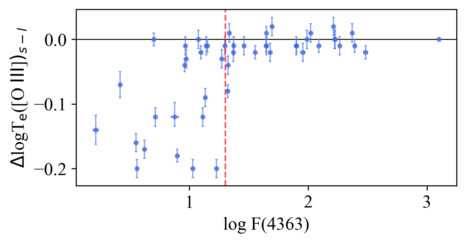
Figure 3: The relation between [O iii] $\lambda$4363 raw fluxes measured from the long exposure and the differences in electron temperatures $\Delta$log T_e derived from diagnostic [O iii] lines using short and long exposures. The $\lambda$4363 raw fluxes, F(4363) are in the units of $10^{-16}\mathrm{erg~{}cm^{-2}s^{-1}}$. The error bars on the data points represent the measurement uncertainty. Both axes are presented on a log scale. It is clear the $\Delta$log T_e values are close to zero until the [O iii] $\lambda$4363 line flux drops below 20 $\times 10^{-16}\mathrm{erg~{}cm^{-2}s^{-1}}$, which is indicated by the red dashed line.

The electron densities, $n_{\mathrm{e}}$, derived from short and long exposures exhibit slightly larger discrepancies compared to those in $T_{\mathrm{e}}$ while the measurement uncertainties in electron densities are usually larger. For the low-ionization zone, the $n_{\mathrm{e}}$ values obtained from [O ii] and [S ii] diagnostic lines in short and long exposure spectra generally agree within 2$\sigma$. The $n_{\mathrm{e}}$([S ii]) values derived from the short-exposure spectra tend to be higher, which might be due to the different extinction corrections applied. Regarding the medium-ionization zone, the $n_{\mathrm{e}}$ values derived from [Cl  iii] and [Ar iv] density diagnostic lines agree within 2$\sigma$ for 72% and 68% of the objects, respectively, as the emission lines for these elements are usually weak. In several cases, line intensities measured from the short-exposure spectra yielded abnormally low densities due to lower s/n. The median differences in resulting $n_{\mathrm{e}}$ values are $0.01_{-0.11}^{+0.23}$ for the low-ionization zone and $0.03_{-0.20}^{+0.59}$ dex for the medium-ionization zones.

4.1.3 Chemical abundance from available lines in short and long exposure spectra

We now compare the elemental abundances derived separately from the short- and long-exposure spectra, wherever possible. Summary results are given in Table 4. The abundance values of a given element are represented on a log scale where $\log$(H)$=12$. Column 2 of the table presents the median differences in derived elemental abundances, along with the uncertainties based on the 16th percentile and 84th percentile values. The number of PNe used in the calculation is indicated in brackets. Overall, the results from short- and long-exposure spectra show a good agreement. Short-exposure spectra tend to yield slightly higher abundance estimates for these elements, with a median difference typically below 0.1 dex. The discrepancies in He/H are minimal, whereas heavier elements display differences greater than 0.5 dex for some individual PNe.

Table 4: The median difference between elemental abundances derived from the short-exposure and long-exposure spectra. Column 1 displays the element concerned. Column 2 provides the median difference, accompanied by the 16th percentile and 84th percentile values, as well as the number of PNe used in the calculation (in brackets). Columns 3 and 4 list the number of PNe with results that agree within 2$\sigma$ and within 0.2 dex, respectively, along with the corresponding fractions in parentheses.

12$+\log$((X/H)	$\Delta_{s-l}$	$\Delta_{s-l}$ $<$ 2$\sigma$	|$\Delta_{s-l}$| $<$ 0.2 dex
He	$-0.00_{-0.04}^{+0.04}$ (70)	46 [0.66]	69 [0.99]
N	$\phantom{-}0.02_{-0.18}^{+0.48}$ (64)	34 [0.53]	39 [0.61]
O	$\phantom{-}0.05_{-0.17}^{+0.28}$ (70)	42 [0.60]	43 [0.61]
Ne	$\phantom{-}0.14_{-0.14}^{+0.53}$ (56)	26 [0.46]	29 [0.52]
S	$\phantom{-}0.05_{-0.41}^{+0.42}$ (69)	44 [0.64]	39 [0.57]
Ar	$\phantom{-}0.04_{-0.16}^{+0.24}$ (70)	35 [0.50]	46 [0.66]
Cl	$\phantom{-}0.11_{-0.20}^{+0.50}$ (62)	36 [0.58]	35 [0.56]

The discrepancies in the elemental abundances are attributed to s/n and the number of detectable emission lines for a given ionic species. The elemental abundance is calculated by multiplying the sum of ionic abundances with the corresponding ICF. To better understand these discrepancies, we examined the correlation between them and differences in individual ionic abundances and ICFs. We regard either the ionic abundance or ICF as responsible for the elemental abundance discrepancy when a strong correlation coefficient ($r>0.5$) is observed.

The observed discrepancies in He/H, O/H, S/H, Ne/H, Ar/H, and Cl/H abundances mainly stem from differences in the abundances of the dominant ions: He⁺/H⁺, O²⁺/H⁺, Ne²⁺/H⁺, S²/H⁺, Ar²⁺/H⁺, and Cl²⁺/H⁺. The calculation of ionic abundances relies solely on the emission line intensity of the ion measured from the spectra and the corresponding line emissivities determined by the physical parameters (Osterbrock & Ferland, 2006). Overall, the agreement in He/H is generally good, with a median difference in He⁺/H⁺ of $0_{-0.06}^{+0.02}$ dex, although some results deviate by more than 0.2 dex due to measurements of weak He i lines or large deviations in electron temperature ($\Delta T_{\mathrm{e}}>0.5$ dex). Similarly, short exposures tend to measure more abundant Cl²⁺, primarily due to [Cl iii] $\lambda\lambda$5517,37 lines being at the red end with poor-s/n, resulting in ineffective removal of background noise pixels. The determination of ionic abundance ratios for O²⁺/H⁺, Ne²⁺/H⁺, S²⁺/H⁺, Ar²⁺/H⁺ and Cl²⁺/H⁺ depends on lines emitted from medium- ionization regions. The strong emission lines from these ions make the differences in measured line intensities between short and long-exposure spectra insignificant in terms of resulting ionic abundances. Our investigation discovered that changes in these abundances exhibit an extremely strong correlation with variations in the derived electron temperatures in the medium-ionization zone, which is consistent with the formula used in neat to calculate ionic abundances. Notably, since Ne²⁺ is the only observable ionisation stage of Ne in our optical spectra, a systematic reduction in electron temperature computed from short exposures, as discussed previously in Sec.4.1.2, results in higher Ne/H values obtained from the short exposures.

We found that the discrepancies in the N/H estimates are mainly associated with the differences in ICFs. Since the dominant ionization stages of nitrogen, N²⁺, manifest in the UV and far-infrared (e.g. Wang & Liu, 2007) and are not detectable in our optical spectra, the ICF accounting for such unobserved ionization stages of nitrogen, icf(N), is typically much larger than unity, compared to other elements. The determination of icf(N) relies on the abundance ratios of O⁺/N⁺. Similar to the previously discussed findings, the difference in N⁺/H⁺ and O⁺/H⁺ are strongly correlated with the difference in electron temperatures in the low-ionization zone, typically used $T_{\mathrm{e}}$([N ii]). However, accounting for the recombination intensities of [N ii] $\lambda$5755 and [O ii] $\lambda$7319,30 introduces further complexities. Thus, precise determination of the ionic abundances of N²⁺ and O²⁺ through ORLs in extensive spectra is essential in accurately calculating both electron temperature and N/H values.

In summary, chemical abundances derived from the short- and long-exposure spectra agree within 2$\sigma$ for over half of the PNe in this study, while a similar fraction of objects show a consistency better than 0.2 dex. This suggests the agreement between high-quality measurements and our error estimation from Monte- Carlo simulations is reasonable. We found that the discrepancy in ionic abundances derived for He, O, Ne, S, Ar or the ICFs applied (for N) primarily result from differences in the measured physical parameters that arise when having to deal with lower s/n spectra. We found that short-exposure spectra tend to give an underestimation of $T_{\mathrm{e}}$ in the medium-ionization zone resulting in slight over-estimations of the abundances of O, Ne and Ar. The differences can be large. Nevertheless, for many PNe our short-exposure spectra can still effectively detect the key emission lines at sufficient s/n that are used to determine the abundance of the dominated ions as the equivalent long-exposures. As the wide $\Delta T_{\mathrm{e}}$ estimates show and their critical correlation with the derived abundances between the short and long exposures, accurate measurement of plasma diagnostics line ratios from the high s/n spectra is essential to the reliability of chemical abundance determinations. The determination of N/H could suffer from large systematic uncertainties as correction for the recombination contribution is needed. In addition, as discussed in Wesson et al. (2018), different ICF schemes could result in a difference up to 20% in N/H. Such errors in ICFs were included in the DMS14 scheme we used in this study. As a result, uncertainties associated with N/H could be larger than that derived using other schemes. This could explain why fewer determinations of N/H agree within 0.2 dex.

4.2 Comparison of the results obtained with the He i lines and [O ii] lines

Multiple He i lines are available across the optical spectra for many PNe sampled in both the blue and red spectrograph arms. A comparison between the He⁺/H⁺ derived from these lines can be used to establish the consistency of the results derived from the two arms. Additionally, O⁺ abundances can be derived from either the blue [O ii] $\lambda\lambda$3726,29 or the red [O ii] $\lambda\lambda$7319,30 doublet. Standard star flux calibration is not available for most of the PNe in our sample in the wavelength range of the blue [O ii] lines, but a comparison between of the results from different lines of the same element can help elucidate factors that cause discrepancy and help to assess the reliability of the O⁺ abundances derived from the red doublet.

4.2.1 The He i lines

The three He i lines at $\lambda\lambda$4471, 5876, 6678 were used in our abundances derivation with weights of 1, 3 and 1 respectively. Two other usually well-represented lines, He i $\lambda\lambda$3889, 7065 result from the decays to 2s³S and 2p³P that are sensitive to opacity effects and so are not used as their observed intensities significantly deviate from the case B approximation predictions (Porter et al., 2005; Blagrave et al., 2007; Del Zanna & Storey, 2022). The photoionization models in Rodríguez (2020) show that He i lines arising from the transitions 2¹P^o-n¹D and 2³P^o-n³D, i.e. He i $\lambda$4026, $\lambda$4388, $\lambda$4471, $\lambda$4922, $\lambda$5876 and $\lambda$6678, are mostly insensitive to optical depth effects so the abundances derived from these lines can be realistically compared with the adopted He⁺/H⁺ results.

The box plots of the differences between He⁺ abundances derived from each He i line and the weighted average abundance implied by the three brightest He i lines, $\lambda$4471, $\lambda$5876 and $\lambda$6678 for the PNe sample are shown in Fig. 4. The median values of the differences between the results from each line and the final adopted value are generally within 0.04 dex. Therefore, each of these He i lines can provide an unbiased estimation of He⁺/H⁺, as demonstrated by the photoionization models in Rodríguez (2020). The spread of discrepancies in the two He i lines, He i $\lambda\lambda$4388, 4922, not used in the derivation, is wider with many more outliers and with some cases showing $\Delta\log$ (He⁺/H⁺) $>0.5$. This is owing to the larger errors from measuring these weaker He i emission lines.

In Fig. 5, we present the same discrepancies in He⁺/H⁺ derived from the multiple He i lines in each PNe spectrum as a function of the raw line fluxes. The orange line shows the median difference in $\log$ (He⁺/H⁺) as a function of He i line fluxes in bins of 0.2 dex, while the shaded region indicates the 16-84th percentile range of the measures. Unsurprisingly, the discrepancy increases as the flux decreases. For lines with log fluxes $<-1$, the median differences is worse than $-0.5$ dex. The black dotted line at $\log$ F(He i) $=-0.15$ marks where the 84th percentile value of each bin becomes positive. All emission lines measured with a flux $\log$ F(He i) $\leq-0.15$ leads to a result lower than the adopted He⁺/H⁺ value.

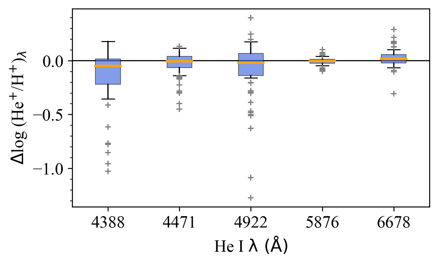
Figure 4: Box plots showing the comparison of He⁺ abundances derived from individual He i lines and the final adopted values for the PNe sample. The final adopted He⁺/H⁺ value for any PNe is the average of the results derived from He i $\lambda\lambda$4471, 5876 and 6678, having corresponding weights of 1, 3 and 1, respectively. Each box spans from the 16th to 84th percentiles, with the median value denoted by orange lines. Whiskers extend to represent the 1st and 99th percentiles, while grey crosses indicate outliers.

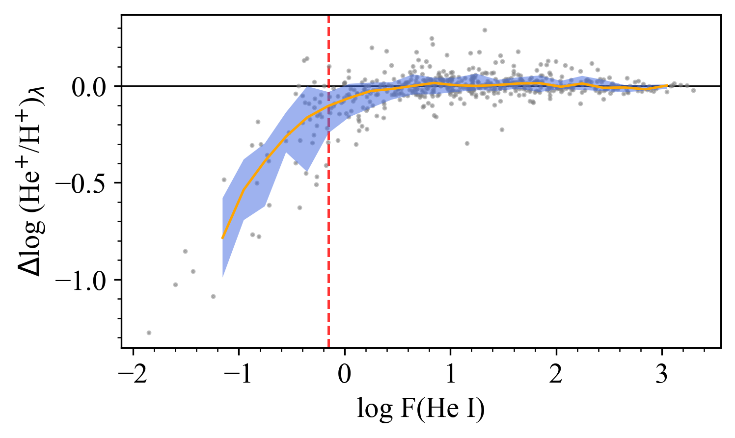
Figure 5: The differences between $\log$ (He⁺/H⁺) values derived from each He i line and the final adopted values are plotted against their raw fluxes ($\log$ F(He i) in the units of $10^{-16}\mathrm{erg~{}cm^{-2}s^{-1}}$) for all measured He i lines across the PNe sample. The light blue shaded region encloses the 16th and 84th percentile of $\Delta\log$ (He⁺/H⁺) in 0.2 dex bins in log F(He i), while the orange curve indicates the median value. The vertical red dashed line at $\log$ F(He i) $=0.15$ shows the demarcation where the 84th percentile value of each bin becomes positive.

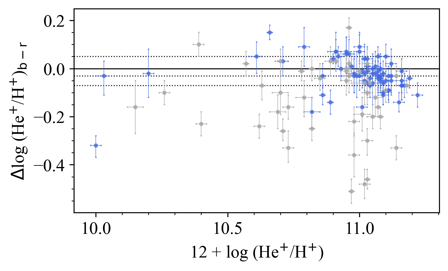
Figure 6: The differences in He⁺ abundances derived from the blue and red spectra. Blue dots correspond to objects with raw fluxes for all He i lines with $\log$ F(He i) $>-0.15$, while grey dots represent those with weaker lines. These unsurprisingly have a greater spread in $\Delta\log$ (He⁺/H⁺). Error bars account for the measurement uncertainties. Grey dashed horizontal lines represent the median difference, as well as the 16th and 84th percentile values.

To further examine whether the He⁺/H⁺ derived from the blue and the red spectral arms are consistent, we averaged the results of He⁺ abundances derived from lines in the blue spectra, namely He i $\lambda\lambda$4388, 4471, 4922, and those in the red spectra, namely He i $\lambda\lambda$5876, 6678. The differences between the results from the He⁺ abundances from lines in the blue and red spectra are plotted versus the adopted He⁺/H⁺ values in Fig. 6. Error bars come from the observed measurement uncertainties. In the plot, the blue dots are for PNe with all He i line fluxes $>0.7\times 10^{-16}\mathrm{erg~{}cm^{-2}s^{-1}}$, therefore, with no significant underestimation in He⁺/H⁺. In this sample 86% of objects have results whose red and blue lines spectra agree within 2$\sigma$. The difference between these results is $-0.01^{+0.07}_{-0.06}$ dex, indicating good consistency. The grey points are for PNe where one or more of the He i line fluxes are less than $0.7\times 10^{-16}\mathrm{erg~{}cm^{-2}s^{-1}}$. Larger discrepancies are seen, as might be expected with the blue spectra results being generally lower. The median difference is $-0.08^{+0.10}_{-0.18}$ dex with this value and associated errors given by the horizontal dotted lines.

The agreement between the He⁺ abundances obtained from the blue and red spectra demonstrates that the scaling factor applied to the red spectra is effective and does not introduce any systematic errors in our abundance calculations, the flux calibration or extinction corrections. It is clear that He i emission lines with a measured flux below $0.7\times 10^{-16}\mathrm{erg~{}cm^{-2}s^{-1}}$ result in an underestimation of ionic abundances. This finding is also likely to be applicable to other elements.

4.2.2 [O ii] lines

In the analysis of PNe oxygen abundances, previous studies (e.g. Viegas & Clegg, 1994; Escudero et al., 2004; Exter et al., 2004) have found that using the [O ii] $\lambda\lambda$7319,30 red emission line pair typically results in a systematically higher O⁺ abundance of up to 1 dex compared to the [O ii] $\lambda\lambda$3726,29 blue line pair. The discrepancy persists even after subtracting the contribution of recombination [O ii] $\lambda\lambda$7319,30 lines, with differences in the results reaching a factor of 2 or more. Most previous studies on PNe oxygen abundances from optical spectra have predominantly used the $\lambda\lambda$3726,29 pair, e.g. Kingsburgh & Barlow (1994) and Magrini et al. (2009), since they are usually bright and can be detected in the spectra with high s/n.

In our total sample, 34 PNe have both the blue and red [O ii] lines present in their spectra. A comparison between the O⁺/H⁺ derived from the red and the blue doublets is shown in Fig. 7. The red doublet [O ii] lines yield O⁺ abundances consistently exceed those from the blue [O ii] doublets by a median value of 0.19 dex. The orange dots represent data points that deviate from the dotted 1-to-1 correspondence line by more than 2$\sigma$ (given the errors on each point). A generally tight relationship is observed, with the O${}^{+}_{\mathrm{b}}$ and O${}^{+}_{\mathrm{r}}$ are correlated with a coefficient $r=0.97$. The solid blue line represents the least-squares best-fit between O${}^{+}_{\mathrm{r}}$ and O${}^{+}_{\mathrm{b}}$, which is derived as $y=1.02x+0.07$ with a $R^{2}=0.97$.

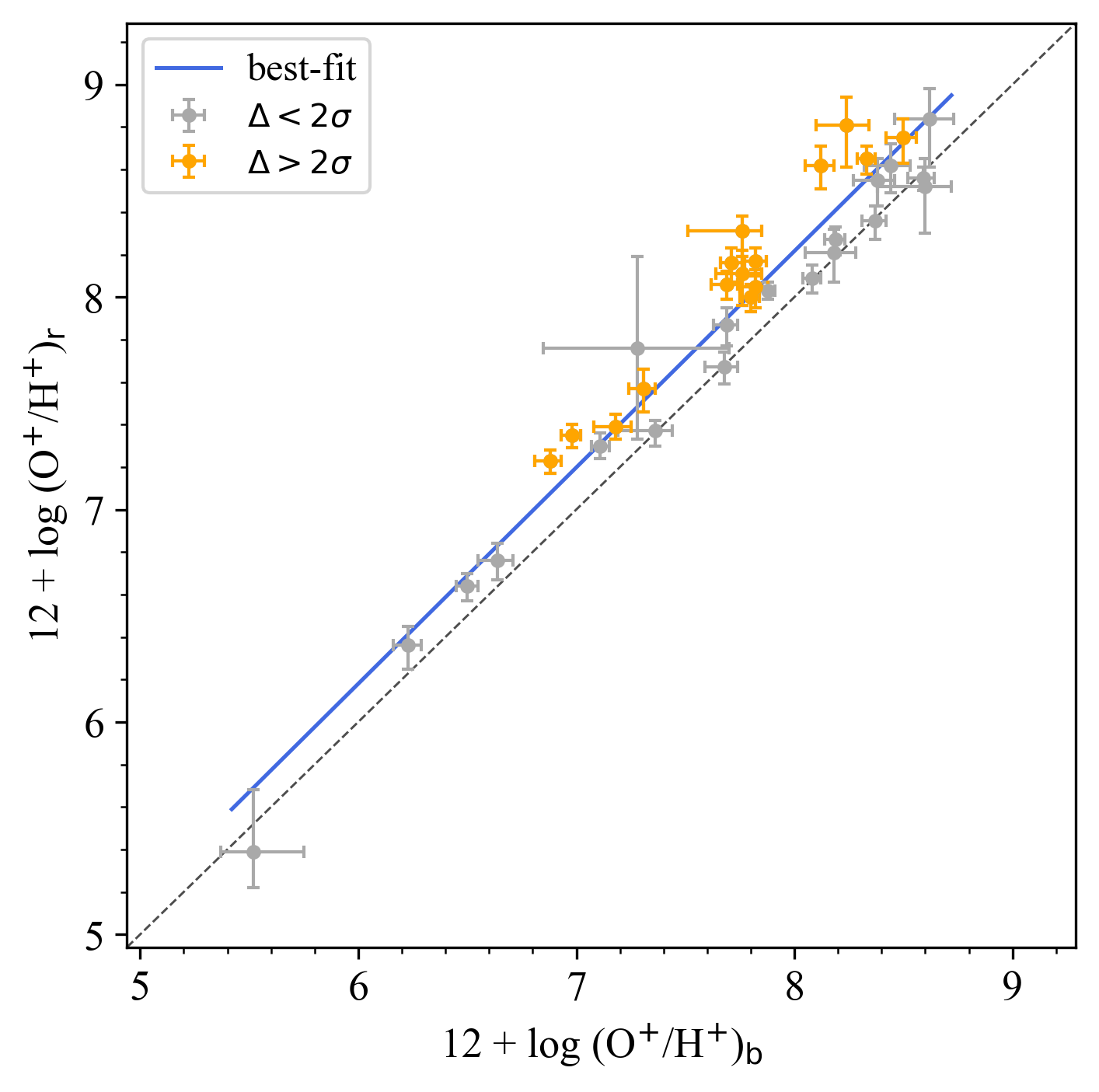
Figure 7: The relationship between ionic abundances of O⁺ derived from the blue [O ii] $\lambda\lambda$3726,29 (subscript ’b’) doublet and the red [O ii] $\lambda\lambda$7319,30 (subscript ’r’) doublet of 34 PNe in this work. The solid blue line shows the best-fit, $y=1.02x+0.07$, while the dotted line represent $y=x$. Orange dots represent the results that do not agree within 2$\sigma$ of $y=x$, taking into account measurement errors.

We assessed whether uncertainties in the blue [O ii] line flux measurements, which are situated at the edge of our spectroscopic images and could be affected by instrument responsivity issues, could result in this discrepancy. No correlation was found between the raw fluxes of [O ii] $\lambda\lambda$3726,29 lines and the O${}^{+}_{\mathrm{r}}$/O${}^{+}_{\mathrm{b}}$ ratios. We noted that higher extinction coefficients estimates obtained using the H$\delta$/H$\gamma$ ratio suggest a potential flux deficit (H$\delta$/H$\gamma$ gives higher c(H$\beta$) than H$\beta$/H$\gamma$ for 85% of PNe) at the blue end. However, the difference between the measured H$\delta$ intensity and the expected value based on c(H$\beta$) obtained from H$\beta$/H$\gamma$ line ratios also show no correlation with O${}^{+}_{\mathrm{r}}$/O${}^{+}_{\mathrm{b}}$. Therefore, these factors may not contribute to the discrepancy.

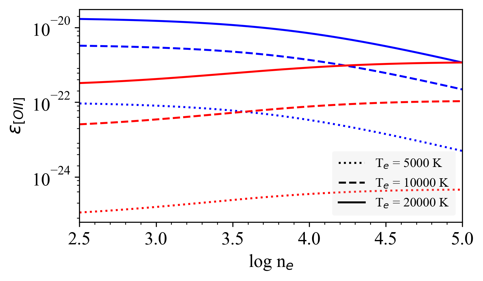
Figure 8: The summed line emissivities, $\epsilon$, of [O ii] $\lambda\lambda$3726,29 (in blue) and [O ii] $\lambda\lambda$7319,30 (in red) emission lines, measured in units of erg$\cdot$s${}^{-1}\cdot$cm³, as a function of electron density in the units of cm^-3, on a log scale. The data was obtained using the getEmissivity commands in PyNeb using the data of Zeippen (1982) and Wiese et al. (1996) for different transitions. The solid, dashed and dotted curves correspond to electron temperatures of 5000, 10,000, and 20,000 K, respectively.

Through a study of H ii regions using deep spectra, Méndez-Delgado et al. (2023) suggested that the presence of high-density clumps in nebulae account for a discrepancy of $\sim 0.1$ dex for H ii regions. While the discrepancy observed in our sample of PNe is larger, it is likely the same underlying cause. Similar to Méndez-Delgado et al. (2023), we found that [O ii] ($\lambda\lambda$7319+30)/($\lambda\lambda$3726+29) line ratio consistently gives higher estimates of $T_{\mathrm{e}}$ than [N ii] lines, with a median difference of $0.29^{+0.21}_{-0.30}$ dex. Among the 34 PNe studied, 12 (35%) have $T_{\mathrm{e}}$([O ii]) at the high-temperature limit of 35,000 K. Fig. 8 presents the change in summed blue and red [O ii] line emissivities as a function of $n_{\mathrm{e}}$. High-density clumps could account for the observed discrepancy in two ways: one is that the measured blue [O ii] lines are strongly biased towards low density regions, similar to [S ii], resulting in an underestimation of the overall electron density and a significant overestimation of [O ii] temperatures. Meanwhile, the emissivity for the blue [O ii] lines in the high density regions is overestimated which lead to an underestimation of the O${}^{+}_{\mathrm{b}}$ abundances. The second is that, as the red [O ii] lines are biased towards high densities, using the lower $n_{\mathrm{e}}$ values estimated from [O ii] and [S ii] could underestimate emissivity and overestimate abundance.

Thus, deriving O⁺ abundances using the blue [O ii] lines may provide fair measurements for the low-density regions while the high-density regions might not be well-represented. In contrast, using the red [O ii] lines suffers from underestimated $n_{\mathrm{e}}$ values, leading to inflated abundances. However, for high-density regions where the red [O ii] lines are enhanced, the actual electron temperature could be lower than the overall $T_{\mathrm{e}}$ estimates using [N ii] lines, their actual emissivity might be lower. This could be a compensate for the accuracy of our final estimations.

To summarise, in our results, the red [O ii] $\lambda\lambda$7319,30 doublet lines consistently yields higher O⁺/H⁺ than the blue [O ii] $\lambda\lambda$3726,28 doublet, possibly due to the presence of condensations in the nebulae. As such, the O${}^{+}_{\mathrm{r}}$ values used for the majority of objects in our study reflect measurements from the dense clumps in the nebulae, if present.

5 Abundance Comparisons with literature results

In this section, we compare our abundance results with some of the most recent published studies, namely WL07, GKA07, GCS09, CCM10, PBS15, and SZG17, which refer to Wang & Liu (2007), Girard et al. (2007), Górny et al. (2009), Cavichia et al. (2010), Pottasch & Bernard-Salas (2015), and Smith et al. (2017), respectively. WL07, GKA07, and CCM10 used 2-m class telescopes, while GCS09 utilised 4-m class telescopes and SZG17 used the VLT. Additionally, PBS15 employed both optical spectra from the literature and mid- infrared observations from Spitzer. Most of these studies made use of low- to medium-resolution spectra while WL07 utilized high-resolution spectra spanning from 3900 Å  to 4980 Å  and SZG17 employed high-resolution VLT/UVES spectra. We excluded earlier work by Escudero et al. (2004) for comparison, as its sample largely overlaps with the later works. Furthermore, we did not include Exter et al. (2004), which used the multi-object spectrograph on 1.2-m telescope, as some literature values for physical conditions were adopted, making the data less homogeneous. To place this comparison on the same footing we derived the elemental abundances using the same ICF scheme introduced in KB94 as used in most of this literature.

Table 5 displays the median differences in elemental abundances, together with uncertainties estimated from the 16th and 84th percentile values, of helium, nitrogen, oxygen, neon, sulphur, argon and chlorine for PNe that are common between this work and seven other literature samples. The median difference in extinction coefficient is also presented in Col. 1. The numbers in brackets following the abundance differences give the number of PNe available for comparison for that particular element. The He/H values show excellent agreement, as the emission lines are usually bright and all the ionization stages can be observed in the optical spectra. The agreement in N/H, O/H, S/H, and Ar/H among the different authors is generally good, with median differences typically below 0.2 dex, except for PBS15 and SZG17, which will be discussed later.

Table 5: Comparison between PNe literature abundances and this work. The differences shown correspond to our results minus the literature values, with median values and uncertainties based on the 16th and 84th percentile values. The number of objects in common with literature studies is indicated in brackets. An asterisk next to WL07 denotes that the recombination contribution has been subtracted from the [N ii] $\lambda$5755, [O ii] $\lambda\lambda$7319,30, and [O iii] $\lambda$4363 intensities. Electron temperatures in PBS15 adopted additional diagnostics from mid-infrared spectra.

Sample	$\Delta$c(H$\beta$)	$\Delta\log$(He/H)	$\Delta\log$(N/H)	$\Delta\log$(O/H)	$\Delta\log$(Ne/H)	$\Delta\log$(S/H)	$\Delta\log$(Ar/H)	$\Delta\log$(Cl/H)
⋆WL07 (10)	$\phantom{-}0.11_{-0.21}^{+0.56}$	$\phantom{-}0.00_{-0.03}^{+0.03}$(10)	$-0.03_{-0.16}^{+0.17}$(10)	$-0.04_{-0.07}^{+0.06}$(10)	$\phantom{-}0.01_{-0.02}^{+0.10}$(10)	$-0.05_{-0.12}^{+0.12}$(10)	$\phantom{-}0.09_{-0.08}^{+0.10}$(10)	$\phantom{-}0.00_{-0.16}^{+0.01}$(10)
GKA07 (6)	$-0.07_{-0.17}^{+0.22}$	$\phantom{-}0.03_{-0.02}^{+0.02}$(6)	$\phantom{-}0.18_{-0.16}^{+0.06}$(6)	$\phantom{-}0.08_{-0.10}^{+0.27}$(6)	$\phantom{-}0.21_{-0.16}^{+0.10}$(5)	$\phantom{-}0.11_{-0.11}^{+0.16}$(6)	$\phantom{-}0.15_{-0.22}^{+0.16}$(6)	$\phantom{-}0.21_{-0.24}^{+0.17}$(6)
GCS09 (40)	$\phantom{-}0.01_{-0.18}^{+0.32}$	$-0.08_{-0.07}^{+0.07}$(40)	$-0.14_{-0.15}^{+0.18}$(37)	$\phantom{-}0.08_{-0.14}^{+0.23}$(40)	$\phantom{-}0.22_{-0.23}^{+0.2}$(30)	$-0.01_{-0.28}^{+0.17}$(36)	$\phantom{-}0.01_{-0.16}^{+0.19}$(39)	$-1.04_{-0.38}^{+0.38}$(27)
CCM10 (15)	$\phantom{-}0.38_{-0.43}^{+0.32}$	$-0.02_{-0.05}^{+0.13}$(15)	$\phantom{-}0.21_{-0.17}^{+0.24}$(14)	$\phantom{-}0.25_{-0.26}^{+0.26}$(15)	$\phantom{-}0.32_{-0.19}^{+0.13}$(12)	$\phantom{-}0.15_{-0.46}^{+0.39}$(15)	$\phantom{-}0.13_{-0.4}^{+0.15}$(14)	-
□PBS15 (8)	$-0.15_{-0.12}^{+0.14}$	$\phantom{-}0.05_{-0.06}^{+0.06}$(8)	$\phantom{-}0.05_{-0.32}^{+0.30}$(8)	$\phantom{-}0.01_{-1.13}^{+0.16}$(8)	$-0.21_{-0.25}^{+0.31}$(4)	$-0.47_{-0.24}^{+0.41}$(8)	$-0.26_{-1.04}^{+0.18}$(7)	$-0.58_{-0.09}^{+0.09}$(2)
SZG17 (6)	$-1.07_{-0.27}^{+0.36}$	$\phantom{-}0.04_{-0.12}^{+0.17}$(6)	$-0.47_{-0.18}^{+0.09}$(6)	$\phantom{-}0.01_{-0.31}^{+0.11}$(6)	-	$-0.33_{-0.45}^{+0.09}$(5)	$\phantom{-}0.48_{-0.45}^{+0.29}$(4)	$-0.64_{-0.43}^{+0.49}$(4)

First we analyse the elemental abundances. It is noteworthy that the data presented in SGZ17 exhibit significant discordance ($>\pm 0.3$ dex) for N/H, S/H, Ar/H and Cl/H in comparison to our work and other published results. The observations were conducted using VLT/UVES, so better agreement with our findings might have been anticipated. We also observed systematical higher extinction coefficients (by 1.07) in SGZ17 compared to our data. As such inconsistencies are not seen when comparing our results with other studies in the literature, it is likely that the extinction coefficients in SGZ17 are substantially overestimated. In comparing raw line fluxes relative to H$\beta$ in SZG17 and our observations, we found their study underestimated blue and overestimated red line fluxes, with magnitude of these deviations exhibiting a positive wavelength dependence. In fact, the wavelength coverage in SZG17 is up to 6680 Å , and the dominant ions of Ar, S, N and Cl are derived from [Ar iv] $\lambda$4711,40, [S iii] $\lambda$6312, [N ii] $\lambda$6548,83 lines and [Cl iii] $\lambda$5517,37 lines. An underestimation of Ar/H is, therefore, likely due to the underestimations of blue [Ar iv] line fluxes. Similarly, over-estimations of S/H, N/H and Cl/H could result from the overestimated red [S iii], [N  ii] and [Cl iii] line fluxes.

We note that the abundances reported in GKA07 and CCM10 (excluding He/H in CCM10) are consistently lower than our findings. In GKA07, the extinction curve by Fitzpatrick (1999) and the KB94 ICF scheme were not employed; instead, the curve by Brocklehurst & Seaton (1972) and ICFs from Aller (1984) and Samland et al. (1992) were adopted. Beyond that, large differences in extinction coefficients and electron temperatures ($>800$ K) are observed when compared to our results. Our data also shows consistently higher abundances ($\geq$0.13 dex) relative to CCM10 for all elements except helium. Similar discrepancies were noticed in CCM10 when compared with earlier works. This is primarily due to the higher electron temperatures used in their study, particularly for the higher ionization zones. The $T_{\mathrm{e}}$ values derived in CCM10 using [N ii] and [O iii] lines were systematically higher than our results, with median values of 1800 K and 3300 K, respectively. We recalculated the physical parameters and chemical abundances using the de-reddened line intensities provided in GKA07 and CCM10, following the methodology employed in this work, to determine whether the procedure deriving the physical parameters, atomic data and assumptions used could explain the discrepancy. For CCM10, the median discrepancies in $T_{\mathrm{e}}$([N ii]) and $T_{\mathrm{e}}$([O iii]) became to 2300 and 2700 K. The discrepancies in elemental abundances for GKA07 and CCM10 persisted, indicating that errors in their extinction correction and line flux measurements, which might be due to the s/n of their spectra, are likely the main cause of this discrepancy.

We observed similar higher electron temperature estimates in GCS09, with median differences of 750 K and 200 K for $T_{\mathrm{e}}$([N ii]) and $T_{\mathrm{e}}$([O iii]), respectively. The use of low-resolution spectra from 4-m class telescopes resulted in smaller discrepancies in derived $T_{\mathrm{e}}$ values compared to CCM10, which used 2-m class telescopes. This highlights the importance of the telescope size in spectral analysis. The values of $T_{\mathrm{e}}$([N ii]) and $T_{\mathrm{e}}$([O iii]) in GCS09 are higher by median values of 550 and $-150$ K when comparing to our results neglecting the recombination corrections for [O iii] and [N ii] auroral lines. When comparing their chemical abundances with our results derived without those recombination corrections, the median differences in O and Ne reduced to less than 0.06 dex. The Cl abundances in GCS09 exhibit the largest discordance, over 1 dex, among all the elements and literature sources examined. We have recalculated the chemical abundances using the de-reddened line intensities in GCS09 and the methods in this study. The median difference in Cl/H significantly reduced to $0.05_{-0.18}^{+0.32}$ and $0.05_{-0.19}^{+0.22}$ dex, respectively compared to our results with and without the recombination corrections. This suggests that the discrepancies in Cl/H are likely due to the atomic data used for Cl. However, the discrepancy in N/H remained after this recalculation even when comparing with our results neglecting the recombination contribution, which is likely attributable to the blending of H$\alpha$ with the [N ii] line, as mentioned in their work.

PBS15 employed alternative diagnostic lines from mid-infrared spectra, making the corrections for recombination in [N ii] $\lambda$5755, [O ii] $\lambda\lambda$7319,30, and [O III] $\lambda$4363 lines unnecessary. The agreement in O/H is good, with a median difference of 0.09 dex. One major advantage of using infrared data is the ability to observe all ionization stages of Ne, S, and Ar, thus eliminating the need for ICFs. Our results for Ne/H, S/H and Ar/H are systematically lower than their results by $>0.20$ dex. These discrepancies are within the uncertainties associated with the KB94 ICF scheme as discussed in DMS14 (at maximum, $\sim 0.2$, 0.4 and 0.7 dex for S and Ar, respectively). However, apart from potential errors in the ICF estimates, this could reflect an underestimation of unobserved ionization stages using ICFs of these elements.

In WL07, the recombination corrections for [N ii], [O ii] and [O iii] auroral lines were carefully addressed. This study also applied similar data reduction approaches and calculation assumptions as in this work. Our results show a good agreement with the abundances from WL07, with discrepancies typically less than 0.05 dex. We compare the ionic abundance measurements for 10 PNe in common to WL07 in the following section to assess the overall quality of our abundance data and explore plausible reasons (such as those mentioned above) for the observed discrepancies.

5.1 Comparison of ionic abundances with the literature results in WL07

There are 10 PNe available for direct comparison between this work and that reported in WL07, i.e. PNG 002.0-06.2, PNG 002.1-04.2, PNG 002.2-09.4, PNG 005.8-06.1, PNG 006.1+08.3, PNG 007.0-06.8, PNG 009.4-09.8, PNG 353.3+06.3, PNG 357.1+03.6, and PNG 359.9-04.5. For both the low- and medium-ionization regions, electron temperatures derived in WL07 and in this work agree well with most differences below 0.05 dex. Electron densities estimates also usually agree within 0.15 dex. The differences in ionic and final elemental abundances between our data and WL07 for the 10 PNe in common are presented in Fig. 9(g) (a-f), together with our measurement uncertainties as error bars. This includes the elements He, N, O, Ne, S, Ar and Cl. Brief comments on the observed differences for the plotted ionic species are given below.

Figure 9: The individual differences in elemental and ionic abundances for 10 PNe derived in this work and common to WL07 for the elements He, N, O, Ne, S, Ar and Cl respectively. PNG numbers of the objects in common with our work are shown in the horizontal axis of the bottom plot for Cl. The error bars are only from uncertainties in this work. Blue circles represent elemental abundances while orange triangles, green diamonds, purple crosses and pink stars indicate the ionic abundances of X⁺/H⁺, X²⁺/H⁺, X³⁺/H⁺, and X⁴⁺/H⁺ respectively. Note that the y-axes have different ranges.

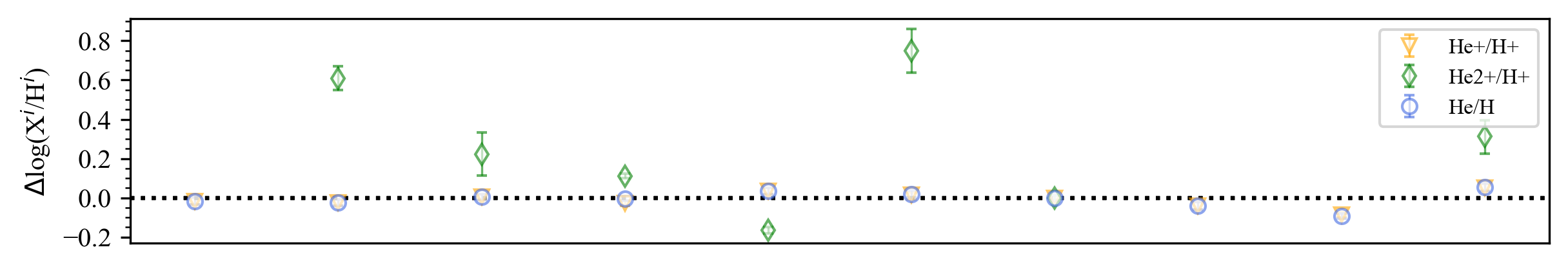
(a) He

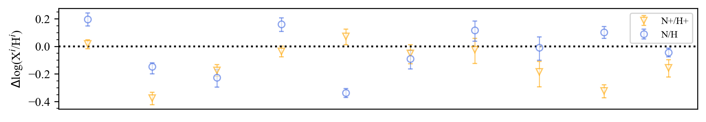
(b) N

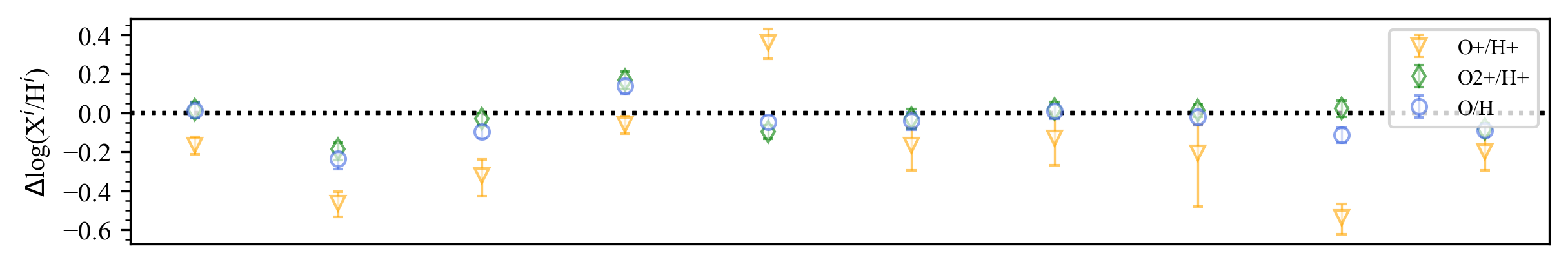
(c) O

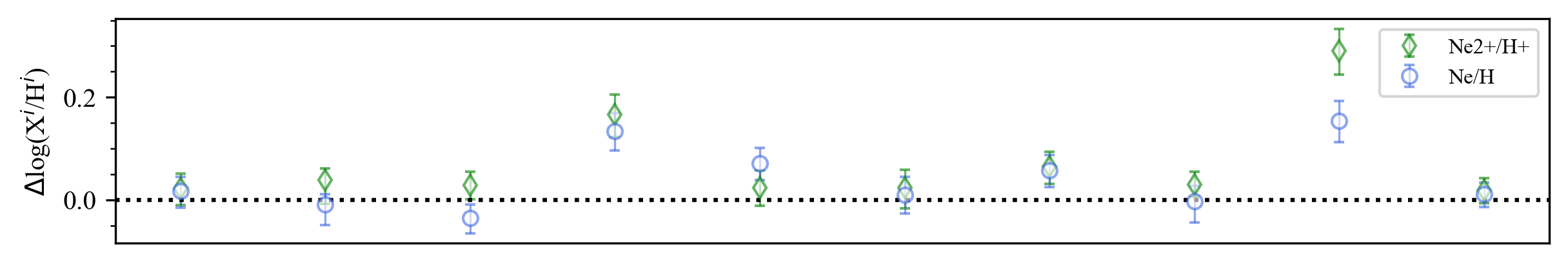
(d) Ne

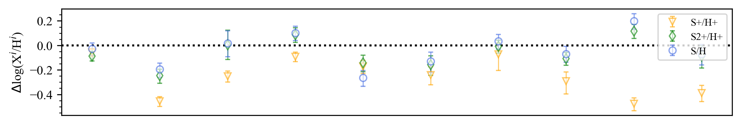
(e) S

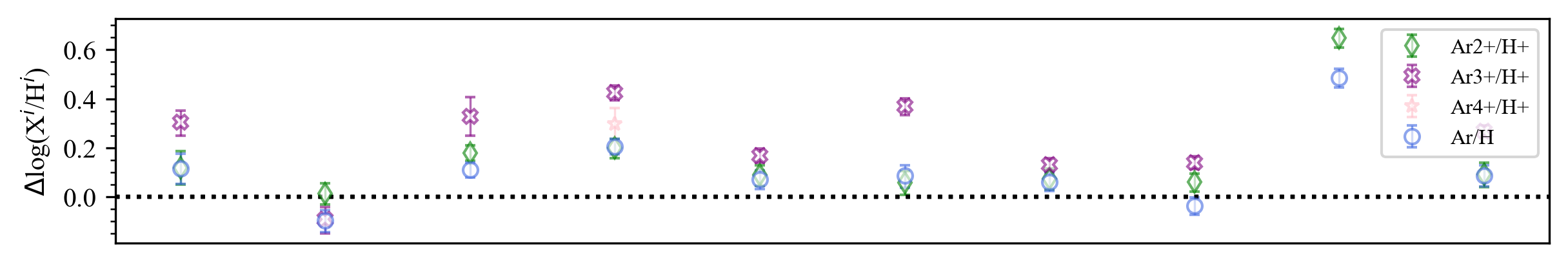
(f) Ar

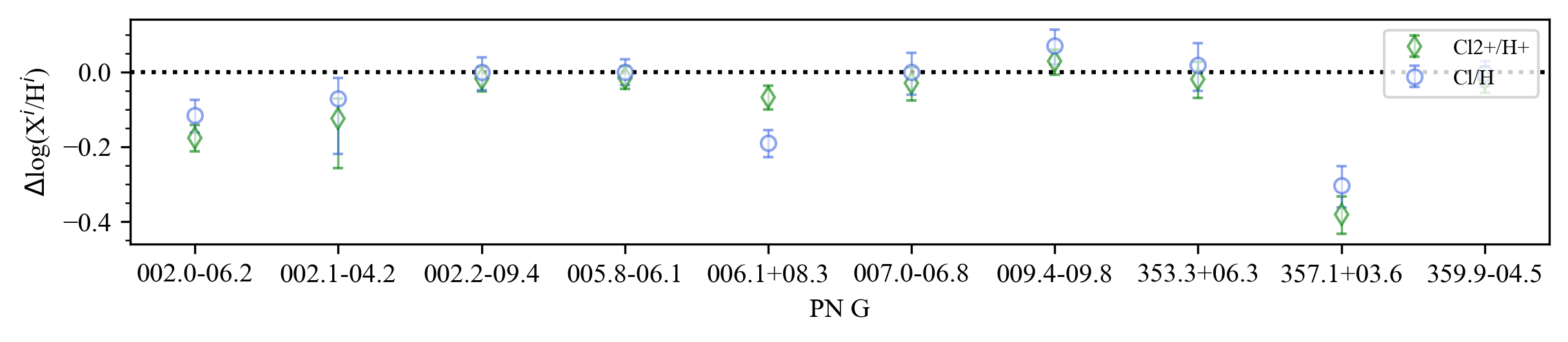
(g) Cl

Helium - the abundance value determined for He is simply the sum of He⁺/H⁺ and He²⁺/H⁺ (which is usually 2-3 dex weaker than He⁺/H⁺). The minor differences of $\leq 0.01$ dex observed between He/H values for 8 PNe are mainly from He⁺/H⁺ measurements, as seen in Fig. 9(a). We weighted the three He i lines, He i $\lambda$4471, $\lambda$5876 and $\lambda$6678 by 1:3:1, as done in WL07. The differences in He⁺/H⁺ arise due to variations in the physical parameters within each PNe. The more uncertain measurements for He ii $\lambda$4686 lines, could account for the larger discrepancies of $>0.5$ dex in He²⁺/H⁺ seen for two PNe.

Nitrogen - the discrepancies in N⁺/H⁺ show a moderately positive correlation with the differences in de-reddened line fluxes and a negative correlation with those in electron temperatures. After comparing our [N ii] line flux measurements with those in WL07, we found that, for most of the objects, the [N ii] $\lambda$6548,83 line intensities in WL07 are higher than our results by up to 45%. This could be due to lower overall extinction coefficients estimated in WL07 and a result of an imperfect deblending of the closely spaced H$\alpha$ and [N ii] emission lines in their low-resolution spectra when [N ii] lines are relatively weaker. For $T_{\mathrm{e}}$([N ii]) values, uncertainties from the detecting weak [N ii] $\lambda$5755 lines and recombination corrections contribute to the discrepancies in individual objects. The difference in N⁺ abundance can partly account for the deviation in N/H. The ICF applied to N also depends on O⁺/H⁺ in the KB94 scheme. As discussed in Sec. 4.1, this also contributes as a large difference in O⁺/H⁺ between our data and the present literature.

Oxygen - the ionic abundance largely depends on the abundance of the dominant ion O²⁺. The determination of O²⁺/H⁺ abundance ratios strongly depends on the measurement of the [O iii] $\lambda$4959, 5007 lines which are not only used for the calculation but also for the derivation of physical parameters. As the two [O iii] lines are usually strong and indeed the strongest nebular lines in un-dereddened PNe, their flux measurement are not often badly affected by spectral quality. The differences in line intensities are generally below 20% when compared with WL07. The O²⁺/H⁺ results usually show good consistency below 0.08 dex. The variations in O²⁺ abundances primarily also stem from differences in $T_{\mathrm{e}}$([O iii]). Upon investigation, these differences in $T_{\mathrm{e}}$([O iii]) show a moderate negative correlation with the difference in extinction coefficients. Most of the O⁺/H⁺ results in WL07 are higher than those in our data, with the discrepancies being highly correlated with the differences in $T_{\mathrm{e}}$([N ii]).

Neon - the observed deviation in neon abundances are small though our results for Ne²⁺/H⁺ are generally higher for most PNe. The [Ne iii]  $\lambda$3868 line intensities in this work are typically higher than those in WL07. The small differences in Ne²⁺/H⁺ seen could be a result of minor line flux measurement errors and different PNe physical parameters derived.

Sulphur - we observed that the differences in S/H between our study and WL07 are greater than 0.2 dex for three objects, which can be attributed to both the S²⁺/H⁺ and icf(S) determined. In both studies, S²⁺/H⁺ was calculated using the [S iii] $\lambda$6312 line. We noted that the difference in S²⁺/H⁺ arise from differences in [S iii] $\lambda$6312 line intensities and electron temperatures. In the comparison, we observed that the line intensities measured in WL07 were consistently higher than our data, typically by $\sim$20%. The ICF of sulphur, similar to that of N, depends on the O/O⁺ ratio, and the discrepancy in S/H can be attributed to the inconsistent results of O⁺/H⁺.

Argon - we observed a systematic increase in both the individual ionic and total elemental abundances of argon compared to the values obtained in WL07, as depicted in Fig. 9(f). The median difference in Ar/H of 0.09 dex is the largest among all the elements. This trend was also observed by Gutenkunst et al. (2008) when comparing their results with those from other literature sources. The elevated Ar/H values were be attributed to several factors, including the observation of Ar³⁺ ions, and uncertainties in $T_{\mathrm{e}}$. Indeed, [Ar iv] lines were observed in both studies for nine PNe while the object, PNG 357.1+03.6, with no [Ar iv] lines observed in WL07 exhibits the largest discrepancy in Ar/H. The differences in Ar²⁺ abundances could primarily result from higher [Ar iii] $\lambda$7135 line intensities measured in this study. This is likely due to the poor instrument detection at the red end of the spectral coverage of WL07 ($\sim$7300-7400Å). The discrepancy diminishes as the electron temperature, $T_{\mathrm{e}}$([O iii]), is higher in our study compared to WL07. Meanwhile, the measured [Ar iv] line intensities show large variations. The discrepancy in Ar³⁺ abundances could be attributed to the differences in electron temperatures, and it is also possible that the higher Ar³⁺/H⁺ values are due to the use of different atomic data, as discussed in Dere et al. (2019).

Chlorine - the abundance of chlorine is a challenging to determine due to the low line fluxes of its dominant ion in the optical region. In column 8 of Table 5, we present the median differences in Cl/H between our data and literature data, which are usually the largest among all elements examined. To derive the chlorine abundance, we used the ICF scheme for chlorine given as

$$\frac{\mathrm{Cl}}{\mathrm{H}}=\frac{\mathrm{S}}{\mathrm{S}^{2+}}\times\frac{\mathrm{Cl}^{2+}}{\mathrm{H}^{+}}$$

in Liu et al. (2000), which was also used in WL07. Upon comparing our results with WL07, as illustrated in Fig. 9(g), we found that the Cl²⁺ ionic abundances generally align well except for PNG 357.1+03.6. The differences in the Cl/H are mainly due to differences in line intensities of [Cl iii] $\lambda$5517,37 and are slightly related to variations in ICFs arising from small differences in S²⁺/S ratios.

In conclusion, we believe that our newly estimated bulge PN abundances for elements He, N, O, Ne, S, Ar and Cl should be more accurate than current literature values for several reasons: i) our spectra exhibit higher s/n ratios, enabling more emission lines to be used for determining ionic abundances compared to prior studies and our enhanced detection of weak emission lines further contributes to the accuracy of our results; ii) we ensured tight instrumental consistency throughout our entire sample; iii) we precisely estimated and incorporated the recombination contribution of specific auroral lines. This is supported by the fact that the chemical abundances derived in this work align most closely with WL07, where recombination abundances were estimated using high-resolution spectra. Furthermore, we used the usually stronger ORLs, specifically, the N ii lines of multiplet V3 measured from our red spectra, which were not employed in WL07; iv) we employed the updated atomic data in chianti 9.0 which is proven to have a better agreement with observations. Also, most of our measurements align with high-quality literature values in WL07 and GCS09 within a 2$\sigma$ range, indicating that our independently estimated measurement uncertainties are reasonable. However, we did encounter larger uncertainties with some older published data, where spectral fitting and s/r may have been problematic. This was especially true when strong line blending occurred in spectra with lower resolutions, resulting in uncertainties in flux measurement that could exceed 40%.

Interestingly, our S/H results show moderate deviation when comparing with literature results using optical spectra while significantly systematically lower than the results from mid-infrared spectra in PBS15, this adds other evidence to an underestimation of higher ionization stages of sulphur in standard photoionization models as pointed out in Kwitter & Henry (2022).

6 General PNe physical conditions and abundance results

6.1 Electron densities and temperatures

The electron densities and temperatures determined from various plasma diagnostic line ratios of 124 PNe in this sample are listed in Table.6. The letters ‘L’ and ‘H’ denote when the measured line ratio exceeds its low- and high-temperature/density limits, respectively. The median electron density for the sample ranges from approximately 2000-$3000$ cm^-3, as determined by different diagnostic lines. These relatively high values are unsurprising given the compact and less evolved nature of the bulge PNe sample.

Table 6: Estimates of the electron density (columns 2-5) and temperature (columns 6-10) derived from all diagnostics lines used in the abundance determination for our PNe sample. Column 1 shows the PNG number for each object. Electron density values are reported in units of cm^-3, and electron temperatures are given in units of K. The upper and lower limits were calculated using the Monte Carlo scheme implemented in neat. We use the letters ‘L’ and ‘H’ to denote low- and high-temperature/density limits, respectively, when the measured line ratio exceeds these values.

PN G	Density diagnostics [cm-3]					Temperature diagnostics [K]
	[O ii]	[S ii]	[Cl iii]	[Ar iv]		[N ii]	[O ii]	[S ii]	[O iii]
000.1+02.6	-	915${}_{-427}^{+315}$	-	1730${}_{-1440}^{+1270}$		-	-	-	9620$\pm$300
000.1+04.3	-	10700${}_{-2100}^{+1600}$	12400${}_{-2100}^{+1800}$	14800${}_{-1500}^{+1300}$		13400$\pm$500	-	28200${}_{-6000}^{+13900}$	11600$\pm$200
000.1-02.3	-	1560${}_{-190}^{+170}$	443${}_{-366}^{+325}$	1800${}_{-580}^{+520}$		-	-	-	11500$\pm$200
000.2-01.9	-	1330${}_{-160}^{+140}$	-	-		6750$\pm$90	-	-	6690$\pm$120
000.2-04.6	-	605$\pm$30	L	L		7690$\pm$120	-	6740${}_{-340}^{+330}$	8160$\pm$130
000.3+06.9	-	219$\pm$56	-	-		-	-	-	-
000.3-04.6	-	1350${}_{-160}^{+140}$	1600${}_{-350}^{+310}$	1560${}_{-570}^{+530}$		7720$\pm$110	-	7350${}_{-560}^{+520}$	9100$\pm$170
000.4-01.9	-	4350${}_{-580}^{+510}$	6170${}_{-790}^{+700}$	-		8830$\pm$170	-	11000${}_{-1900}^{+1400}$	7210$\pm$120
000.4-02.9	-	2440${}_{-1820}^{+980}$	-	L		8470$\pm$270	-	-	8130$\pm$120
000.7+03.2	-	2230${}_{-790}^{+550}$	3230${}_{-370}^{+330}$	2430${}_{-860}^{+820}$		7340$\pm$270	-	-	8590$\pm$160
000.7-02.7	-	407${}_{-97}^{+86}$	7380${}_{-2640}^{+1950}$	6540${}_{-960}^{+840}$		13200$\pm$600	-	H	12600$\pm$300
000.7-07.4	-	392${}_{-340}^{+249}$	448${}_{-376}^{+320}$	L		9000$\pm$230	-	7520${}_{-980}^{+870}$	8970$\pm$170
000.9-02.0	-	2730${}_{-470}^{+400}$	1860${}_{-490}^{+460}$	3290${}_{-680}^{+620}$		7610${}_{-3720}^{+1890}$	-	-	9280$\pm$190
000.9-04.8	-	1440${}_{-160}^{+140}$	519${}_{-340}^{+305}$	1670${}_{-550}^{+520}$		10700$\pm$300	-	9180${}_{-880}^{+800}$	11100$\pm$200
001.1-01.6	-	1050${}_{-310}^{+240}$	3140${}_{-410}^{+360}$	L		8190$\pm$140	-	7200${}_{-600}^{+560}$	8210$\pm$90
001.2+02.1	-	3160${}_{-380}^{+340}$	3510${}_{-1060}^{+850}$	585${}_{-569}^{+533}$		10700$\pm$400	-	22100${}_{-12900}^{+6100}$	8500$\pm$120
001.2-03.0	-	3840${}_{-660}^{+570}$	-	-		5920$\pm$100	-	8550${}_{-1090}^{+910}$	-
001.3-01.2	-	2830${}_{-1770}^{+940}$	9560${}_{-9560}^{+4210}$	-		6640${}_{-140}^{+150}$	-	-	-
001.4+05.3	-	2920${}_{-390}^{+340}$	1140${}_{-820}^{+700}$	-		7800$\pm$160	-	-	7940$\pm$180
001.6-01.3	-	8160${}_{-8160}^{+3240}$	2050${}_{-930}^{+760}$	7500${}_{-1370}^{+1160}$		10200${}_{-600}^{+800}$	-	-	9220$\pm$220
001.7+05.7	-	1030${}_{-130}^{+110}$	L	1600${}_{-510}^{+480}$		12500$\pm$600	-	-	16000$\pm$400
001.7-04.4	-	2720${}_{-410}^{+350}$	4140${}_{-1680}^{+1190}$	-		5870$\pm$90	-	6270${}_{-430}^{+410}$	-
002.0-06.2	2200${}_{-350}^{+300}$	2700${}_{-340}^{+300}$	1140${}_{-710}^{+570}$	-		9460$\pm$190	H	6820${}_{-310}^{+300}$	8110$\pm$110
002.1-02.2	-	5090${}_{-770}^{+670}$	3470${}_{-370}^{+340}$	7250${}_{-650}^{+600}$		12100$\pm$300	-	6280${}_{-550}^{+500}$	10600$\pm$200
002.1-04.2	-	8350${}_{-590}^{+550}$	24100${}_{-22300}^{+8600}$	-		13600$\pm$300	-	H	10300${}_{-200}^{+300}$
002.2-09.4	-	3300${}_{-630}^{+530}$	3930${}_{-1200}^{+920}$	-		9040$\pm$210	-	10700${}_{-1400}^{+1300}$	8880$\pm$110
002.3+02.2	-	672${}_{-208}^{+173}$	-	-		8950$\pm$220	-	-	-
002.5-01.7	976${}_{-273}^{+213}$	479${}_{-152}^{+137}$	-	L		9200$\pm$260	12500${}_{-1100}^{+1000}$	-	8490$\pm$120
002.6+02.1	-	1760${}_{-320}^{+270}$	14300${}_{-5400}^{+4100}$	24100$\pm$1100		8980$\pm$60	-	-	7590${}_{-150}^{+210}$
002.7-04.8	-	1020${}_{-120}^{+110}$	1150${}_{-360}^{+330}$	L		9970$\pm$170	-	-	9000$\pm$160
002.8+01.7	6360${}_{-1760}^{+1250}$	4350${}_{-720}^{+620}$	3350${}_{-460}^{+400}$	-		7100$\pm$100	9330${}_{-1100}^{+910}$	5000$\pm$10	-
002.8+01.8	682${}_{-315}^{+234}$	575${}_{-147}^{+127}$	-	-		9150$\pm$200	8950${}_{-740}^{+680}$	5000$\pm$10	-
002.9-03.9	1830${}_{-460}^{+370}$	12400${}_{-8500}^{+3900}$	L	1110${}_{-640}^{+590}$		-	H	5000${}_{-380}^{+10}$	13200$\pm$200
003.2-06.2	4990${}_{-1210}^{+890}$	2870${}_{-400}^{+350}$	4270${}_{-610}^{+540}$	4140${}_{-790}^{+660}$		9610${}_{-250}^{+240}$	12400${}_{-1900}^{+1500}$	11000${}_{-2000}^{+1500}$	8800$\pm$160
003.6-02.3	864${}_{-198}^{+161}$	931${}_{-180}^{+151}$	L	L		8510$\pm$140	H	6680${}_{-350}^{+330}$	8840$\pm$210
003.7+07.9	-	563${}_{-107}^{+90}$	-	-		5000$\pm$10	-	-	13700$\pm$200
003.7-04.6	-	3420${}_{-590}^{+500}$	1150${}_{-580}^{+520}$	L		19400${}_{-3000}^{+2600}$	-	14400${}_{-6200}^{+3200}$	10900$\pm$200
003.8-04.3	-	2030${}_{-240}^{+220}$	1400${}_{-240}^{+210}$	1680${}_{-480}^{+470}$		9330$\pm$160	-	8240${}_{-530}^{+500}$	10800$\pm$200
003.9-02.3	-	3860${}_{-500}^{+450}$	5750${}_{-900}^{+780}$	4850${}_{-770}^{+670}$		8400$\pm$100	-	8770${}_{-830}^{+760}$	8460$\pm$100
003.9-03.1	-	2680${}_{-910}^{+610}$	3030${}_{-1590}^{+1170}$	1310${}_{-490}^{+470}$		-	-	-	13200$\pm$300
004.0-03.0	-	3030${}_{-400}^{+350}$	2370${}_{-390}^{+330}$	-		14000$\pm$400	-	9720${}_{-930}^{+850}$	H
004.1-03.8	-	1630${}_{-180}^{+160}$	1310${}_{-480}^{+410}$	829${}_{-498}^{+467}$		10600$\pm$200	-	7870${}_{-680}^{+620}$	11100$\pm$200
004.2-03.2	-	1440${}_{-700}^{+490}$	L	601${}_{-513}^{+472}$		13300${}_{-1600}^{+1400}$	-	-	11400$\pm$300
004.2-04.3	-	4110${}_{-500}^{+450}$	3560${}_{-1290}^{+1110}$	1610${}_{-480}^{+460}$		21400${}_{-2400}^{+2000}$	-	-	9740$\pm$190
004.6+06.0	-	3610${}_{-450}^{+400}$	2300${}_{-690}^{+530}$	-		8270$\pm$140	-	-	6690$\pm$160
004.8+02.0	-	5610${}_{-2130}^{+1340}$	L	-		9570${}_{-290}^{+300}$	-	-	8200$\pm$270
004.8-05.0	-	1650${}_{-460}^{+360}$	565${}_{-295}^{+279}$	L		14900$\pm$700	-	-	8570$\pm$210
005.0-03.9	1460${}_{-580}^{+410}$	387${}_{-97}^{+86}$	-	1460${}_{-1330}^{+1210}$		17800$\pm$900	33700${}_{-1300}^{+8800}$	-	23400$\pm$1100
005.2+05.6	-	4040${}_{-600}^{+530}$	844${}_{-239}^{+224}$	1260${}_{-490}^{+460}$		10700$\pm$200	-	7970${}_{-840}^{+760}$	8490$\pm$140
005.5+06.1	-	565${}_{-239}^{+193}$	4750${}_{-1630}^{+1250}$	-		6670$\pm$140	-	-	-
005.5-04.0	-	1390${}_{-190}^{+160}$	1540${}_{-1540}^{+1150}$	763${}_{-437}^{+401}$		-	-	-	10200$\pm$300
005.8-06.1	2660${}_{-600}^{+490}$	2890${}_{-370}^{+330}$	2860${}_{-500}^{+430}$	2560${}_{-460}^{+440}$		8720$\pm$140	19800${}_{-10900}^{+4100}$	7620${}_{-520}^{+490}$	9060$\pm$150
006.1+08.3	-	6050${}_{-980}^{+850}$	10800${}_{-1400}^{+1200}$	16600${}_{-1600}^{+1400}$		10900$\pm$300	-	H	10400$\pm$200
006.4+02.0	-	7840${}_{-1430}^{+1210}$	11700${}_{-1600}^{+1400}$	9330${}_{-1250}^{+1100}$		9490$\pm$200	-	24300${}_{-10700}^{+9700}$	7690$\pm$100
006.4-04.6	-	1240${}_{-150}^{+130}$	123${}_{-123}^{+122}$	1020${}_{-540}^{+530}$		11100$\pm$500	-	-	12800$\pm$300 -

Table 7: continued

PN G	Density diagnostics [cm-3]					Temperature diagnostics [K]
	[O ii]	[S ii]	[Cl iii]	[Ar iv]		[N ii]	[O ii]	[S ii]	[O iii]
006.8+02.3	-	3040${}_{-360}^{+320}$	1340${}_{-450}^{+420}$	4860${}_{-1050}^{+860}$		12200$\pm$300	-	11000${}_{-1700}^{+1300}$	14200$\pm$400
006.8-03.4	3950${}_{-1680}^{+1050}$	7540${}_{-470}^{+450}$	-	4150${}_{-310}^{+290}$		10400${}_{-300}^{+200}$	34600${}_{-400}^{+8100}$	9600${}_{-890}^{+880}$	12200$\pm$100
007.0+06.3	-	4660${}_{-1540}^{+1050}$	2390${}_{-680}^{+530}$	L		9070${}_{-290}^{+280}$	-	6510${}_{-1040}^{+860}$	7510$\pm$120
007.0-06.8	3070${}_{-1210}^{+750}$	2080${}_{-670}^{+510}$	2110${}_{-880}^{+740}$	6570${}_{-1060}^{+910}$		8220$\pm$340	20700${}_{-5200}^{+4100}$	13000${}_{-3300}^{+2300}$	8180$\pm$150
007.5+07.4	-	706${}_{-162}^{+132}$	L	L		8020$\pm$140	-	9860${}_{-960}^{+870}$	9290$\pm$170
007.6+06.9	-	1280${}_{-170}^{+150}$	824${}_{-320}^{+300}$	1090${}_{-510}^{+490}$		9760$\pm$160	-	8670${}_{-820}^{+750}$	10600$\pm$100
007.8-03.7	-	685${}_{-108}^{+94}$	8260${}_{-3120}^{+2640}$	1120${}_{-220}^{+200}$		7620$\pm$170	-	7730${}_{-530}^{+500}$	9110$\pm$120
007.8-04.4	4180${}_{-1240}^{+850}$	7200${}_{-2100}^{+1410}$	-	-		5930$\pm$150	6760$\pm$440	6520${}_{-610}^{+560}$	-
008.2+06.8	-	9750${}_{-2110}^{+1730}$	2540${}_{-460}^{+390}$	-		13400$\pm$400	-	33900${}_{-1100}^{+12200}$	19700${}_{-600}^{+500}$
008.4-03.6	-	570${}_{-193}^{+168}$	-	-		5980$\pm$100	-	5000${}_{-180}^{+10}$	-
008.6-02.6	-	8650${}_{-8440}^{+3190}$	1160${}_{-590}^{+490}$	7310${}_{-1670}^{+1360}$		10100${}_{-500}^{+700}$	-	-	10900$\pm$200
009.4-09.8	-	2870${}_{-1670}^{+1060}$	1990${}_{-380}^{+350}$	1510${}_{-490}^{+460}$		10800$\pm$500	-	-	8780$\pm$140
009.8-04.6	-	1360${}_{-380}^{+300}$	L	1530${}_{-580}^{+540}$		9370$\pm$260	-	12800${}_{-2200}^{+1700}$	9870$\pm$240
351.1+04.8	-	4990${}_{-960}^{+810}$	5480${}_{-900}^{+770}$	-		7900$\pm$130	-	12100${}_{-2700}^{+1900}$	7540$\pm$100
351.2+05.2	-	1390${}_{-190}^{+170}$	2220${}_{-280}^{+250}$	-		5990$\pm$60	-	5000$\pm$10	6870$\pm$160
351.6-06.2	-	1440${}_{-180}^{+160}$	1290${}_{-290}^{+260}$	1180${}_{-450}^{+430}$		8020$\pm$170	-	7610${}_{-430}^{+400}$	10100$\pm$100
351.9+09.0	-	1160${}_{-1130}^{+620}$	336${}_{-336}^{+335}$	1100${}_{-620}^{+570}$		-	-	-	12800$\pm$200
351.9-01.9	8130${}_{-6250}^{+2690}$	5230${}_{-940}^{+800}$	3510${}_{-220}^{+210}$	21600${}_{-1700}^{+1600}$		11900${}_{-300}^{+400}$	16000${}_{-4100}^{+3800}$	14900${}_{-7600}^{+4800}$	9520$\pm$70
352.0-04.6	-	3750${}_{-480}^{+430}$	6010${}_{-770}^{+680}$	4440${}_{-800}^{+680}$		8640$\pm$160	-	10600${}_{-1600}^{+1200}$	8830$\pm$150
352.1+05.1	3620${}_{-750}^{+560}$	3100${}_{-130}^{+120}$	4700${}_{-350}^{+330}$	5010${}_{-340}^{+320}$		8290$\pm$100	20700${}_{-2900}^{+2200}$	10100$\pm$600	8980$\pm$50
352.6+03.0	3110${}_{-1930}^{+1000}$	4070${}_{-260}^{+240}$	8880${}_{-1650}^{+1390}$	14100$\pm$900		8290$\pm$130	H	10500${}_{-1600}^{+1500}$	7960$\pm$70
353.2-05.2	164$\pm$56	113${}_{-56}^{+51}$	-	L		7720$\pm$130	H	5880${}_{-390}^{+360}$	9320$\pm$170
353.3+06.3	-	5340${}_{-910}^{+780}$	3620${}_{-2240}^{+1520}$	7920${}_{-1820}^{+1480}$		10600${}_{-800}^{+900}$	-	19200${}_{-14900}^{+4800}$	9960$\pm$140
353.7+06.3	851${}_{-376}^{+261}$	514${}_{-310}^{+234}$	L	-		6950$\pm$160	10300${}_{-1000}^{+900}$	6290${}_{-470}^{+440}$	7070$\pm$90
354.5+03.3	-	11300${}_{-7400}^{+3500}$	11900${}_{-1400}^{+1300}$	10200${}_{-1100}^{+1000}$		15200${}_{-900}^{+1300}$	-	32400${}_{-2600}^{+4100}$	10600$\pm$100
354.9+03.5	-	2730${}_{-390}^{+340}$	1930${}_{-520}^{+450}$	-		7690$\pm$180	-	6710${}_{-500}^{+460}$	-
355.4-02.4	3580${}_{-840}^{+680}$	3610${}_{-470}^{+420}$	6740${}_{-900}^{+790}$	10700${}_{-1100}^{+1000}$		8330$\pm$130	17100${}_{-2200}^{+1900}$	10500${}_{-1400}^{+1100}$	8410$\pm$120
355.9+03.6	-	18000${}_{-16100}^{+5900}$	-	-		14300${}_{-1100}^{+2000}$	-	28300${}_{-3500}^{+2200}$	10400${}_{-200}^{+300}$
355.9-04.2	-	5930${}_{-260}^{+250}$	4340${}_{-1230}^{+960}$	-		6380$\pm$260	-	7100${}_{-300}^{+290}$	6290$\pm$70
356.1-03.3	-	317${}_{-68}^{+56}$	697${}_{-147}^{+137}$	3730${}_{-760}^{+710}$		8870$\pm$130	-	8840${}_{-540}^{+510}$	9130$\pm$180
356.3-06.2	-	235${}_{-102}^{+97}$	L	1390${}_{-900}^{+820}$		8730$\pm$150	-	-	9430$\pm$130
356.5-03.6	-	3570${}_{-1060}^{+820}$	3120${}_{-600}^{+510}$	3660${}_{-700}^{+650}$		8030$\pm$200	-	-	9040$\pm$190
356.8+03.3	-	4440${}_{-420}^{+380}$	-	-		6850$\pm$100	-	-	-
356.8-05.4	-	336${}_{-112}^{+107}$	L	L		7860$\pm$160	-	-	9100$\pm$140
356.9+04.4	3370${}_{-870}^{+630}$	6560${}_{-820}^{+730}$	14900${}_{-4200}^{+3300}$	33800${}_{-5600}^{+4800}$		14000$\pm$400	H	H	12200$\pm$300
357.0+02.4	-	1870${}_{-270}^{+240}$	1610${}_{-390}^{+340}$	L		8650$\pm$130	-	-	8830$\pm$190
357.1+03.6	-	4010${}_{-730}^{+620}$	1470${}_{-890}^{+700}$	-		8430$\pm$180	-	H	7220$\pm$130
357.1+04.4	-	1200${}_{-270}^{+220}$	-	L		8260$\pm$360	-	-	7880$\pm$320
357.1-04.7	2130${}_{-240}^{+220}$	6680${}_{-1510}^{+1100}$	-	-		5590$\pm$190	9720${}_{-810}^{+750}$	15700${}_{-3900}^{+2800}$	-
357.2+02.0	-	3110${}_{-670}^{+550}$	1090${}_{-480}^{+420}$	2800${}_{-710}^{+670}$		9730${}_{-270}^{+260}$	-	9710${}_{-1430}^{+1140}$	10100$\pm$200
357.3+04.0	-	6900${}_{-2000}^{+1380}$	18400${}_{-6700}^{+4700}$	2120${}_{-640}^{+580}$		11900${}_{-700}^{+600}$	-	-	8160$\pm$100
357.5+03.1	-	1450${}_{-280}^{+240}$	-	-		13300${}_{-1000}^{+900}$	-	-	-
357.5+03.2	-	1610${}_{-340}^{+280}$	-	L		8860$\pm$220	-	-	11000$\pm$300
357.6-03.3	-	352${}_{-107}^{+97}$	-	-		7370$\pm$220	-	-	-
357.9-03.8	-	2770${}_{-1800}^{+1030}$	-	L		21700${}_{-2000}^{+1800}$	-	-	21100$\pm$700
357.9-05.1	-	872${}_{-113}^{+100}$	590${}_{-274}^{+269}$	926${}_{-605}^{+569}$		8620$\pm$190	-	8360${}_{-580}^{+550}$	9160$\pm$130
358.0+09.3	-	377${}_{-377}^{+269}$	631${}_{-631}^{+630}$	L		-	-	-	10200$\pm$200
358.2+03.5	1850${}_{-1850}^{+850}$	6770${}_{-1020}^{+880}$	5400${}_{-820}^{+710}$	9410${}_{-1080}^{+970}$		13300$\pm$400	23800${}_{-11200}^{+6300}$	H	11100$\pm$300
358.2+04.2	1970${}_{-290}^{+250}$	8530${}_{-2110}^{+1540}$	3610${}_{-590}^{+500}$	5620${}_{-3540}^{+3120}$		9350$\pm$200	11300${}_{-1200}^{+1100}$	15100${}_{-5800}^{+3200}$	7980$\pm$90
358.5+02.9	-	2350${}_{-370}^{+320}$	-	1650${}_{-710}^{+590}$		-	-	-	11900$\pm$200
358.5-04.2	6820${}_{-3200}^{+1750}$	8120${}_{-1630}^{+1250}$	12400${}_{-2700}^{+2200}$	-		12600$\pm$400	22800${}_{-8700}^{+5200}$	H	9660$\pm$160
358.6+07.8	3170${}_{-820}^{+650}$	2390${}_{-340}^{+300}$	1050${}_{-380}^{+340}$	1600${}_{-460}^{+440}$		12400$\pm$400	H	11900${}_{-1600}^{+1300}$	8520$\pm$90
358.6-05.5	518${}_{-144}^{+112}$	97${}_{-50}^{+45}$	L	1970${}_{-1290}^{+1140}$		8810$\pm$210	H	7600${}_{-390}^{+370}$	9400$\pm$120
358.7+05.2	2490${}_{-1530}^{+830}$	6550${}_{-1400}^{+1040}$	-	-		6250${}_{-120}^{+130}$	7310${}_{-7310}^{+710}$	7190${}_{-950}^{+840}$	-
358.8+03.0	-	1980${}_{-200}^{+190}$	2820${}_{-990}^{+850}$	1290${}_{-560}^{+520}$		8000$\pm$180	-	8730${}_{-690}^{+640}$	10400$\pm$200
358.9+03.4	-	10700$\pm$600	11300${}_{-1100}^{+1000}$	-		9850$\pm$180	-	32700${}_{-1200}^{+12200}$	7000$\pm$50
359.0-04.1	-	965${}_{-166}^{+141}$	L	814${}_{-630}^{+533}$		8450$\pm$140	-	7820${}_{-540}^{+500}$	8650$\pm$180
359.1-02.9	1150${}_{-190}^{+170}$	1070${}_{-270}^{+210}$	1330$\pm$1330	L		7420$\pm$210	H	5000$\pm$10	7990$\pm$150

Table 8: continued

PN G	Density diagnostics [cm-3]					Temperature diagnostics [K]
	[O ii]	[S ii]	[Cl iii]	[Ar iv]		[N ii]	[O ii]	[S ii]	[O iii]
359.2+04.7	5410${}_{-1640}^{+1100}$	8790${}_{-8010}^{+3070}$	10700${}_{-1900}^{+1600}$	-		9690${}_{-300}^{+400}$	H	7440${}_{-1400}^{+1420}$	-
359.3-01.8	9070${}_{-5880}^{+2710}$	5290${}_{-1190}^{+890}$	L	-		6420${}_{-260}^{+280}$	5860${}_{-440}^{+540}$	6950${}_{-940}^{+1050}$	-
359.6-04.8	-	362${}_{-178}^{+152}$	-	1030${}_{-650}^{+570}$		19400${}_{-1200}^{+1100}$	-	-	13000$\pm$300
359.7-01.8	1830${}_{-1450}^{+740}$	1780${}_{-1210}^{+720}$	L	1520${}_{-680}^{+660}$		7710${}_{-2630}^{+2110}$	H	-	12500$\pm$300
359.8+02.4	-	5870${}_{-1580}^{+1100}$	12700${}_{-9200}^{+4400}$	-		6700$\pm$100	-	5000$\pm$10	-
359.8+03.7	-	5290${}_{-830}^{+720}$	2330${}_{-1340}^{+980}$	-		9800${}_{-660}^{+610}$	-	-	8830$\pm$160
359.8+05.2	67$\pm$55	219${}_{-31}^{+27}$	-	-		-	7440$\pm$310	-	-
359.8+05.6	3910${}_{-960}^{+770}$	7520${}_{-2130}^{+1400}$	6410${}_{-6070}^{+3280}$	-		6270$\pm$260	7660${}_{-710}^{+600}$	7870${}_{-1000}^{+890}$	-
359.8+06.9	999${}_{-361}^{+265}$	826${}_{-178}^{+147}$	4360${}_{-1690}^{+1220}$	-		9900$\pm$160	10100${}_{-900}^{+800}$	6120${}_{-430}^{+410}$	9630$\pm$120
359.8-07.2	-	8260${}_{-3680}^{+2120}$	1100${}_{-1000}^{+800}$	3770${}_{-640}^{+600}$		16100${}_{-3200}^{+2500}$	-	-	11800$\pm$200
359.9-04.5	5560${}_{-1470}^{+1030}$	4620${}_{-770}^{+660}$	9710${}_{-1460}^{+1270}$	16600${}_{-2000}^{+1800}$		9560$\pm$230	H	20300${}_{-14700}^{+5800}$	8430$\pm$110 -

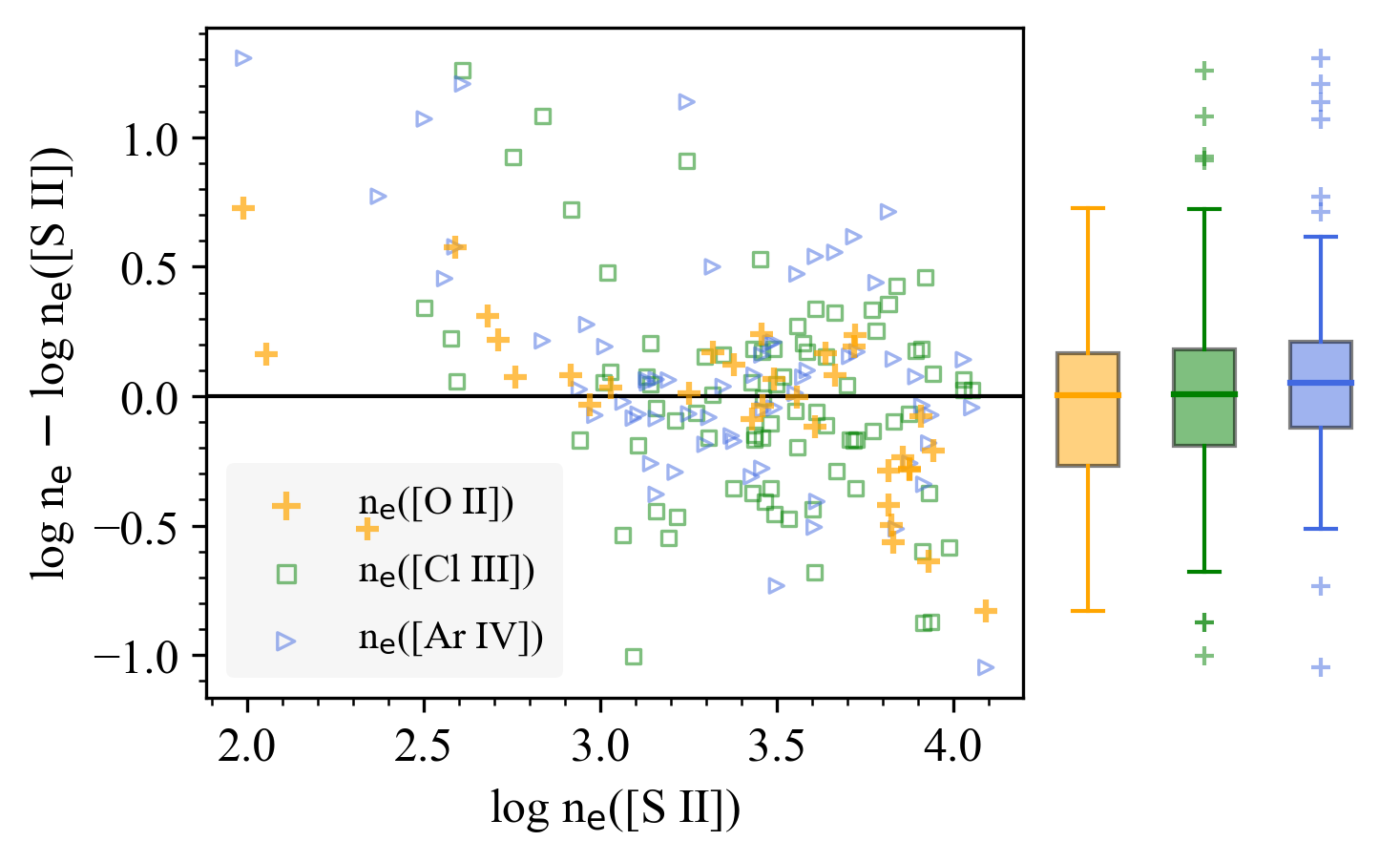
Figure 10: Comparison of electron density estimates using different doublet lines with those derived using [S ii] doublet lines. Electron densities in the units of cm^-3 are shown on a log scale, with values beyond the low or high limits excluded. The scatter plot displays the difference between electron density estimates using [O ii] (orange crosses), [Cl iii] (green squares) and [Ar iv] (blue triangles) compared to estimates from the [S ii] lines, plotted against electron density estimates using [S ii] lines. The black horizontal line marks the zero point. The box plots on the right show the distribution of the differences in electron density estimates, color-coded accordingly. The boxes depict the 25th to 75th percentiles, with the median indicated by a horizontal line. The whiskers extend to the 10th and 90th percentile, and outliers are represented by individual crosses.

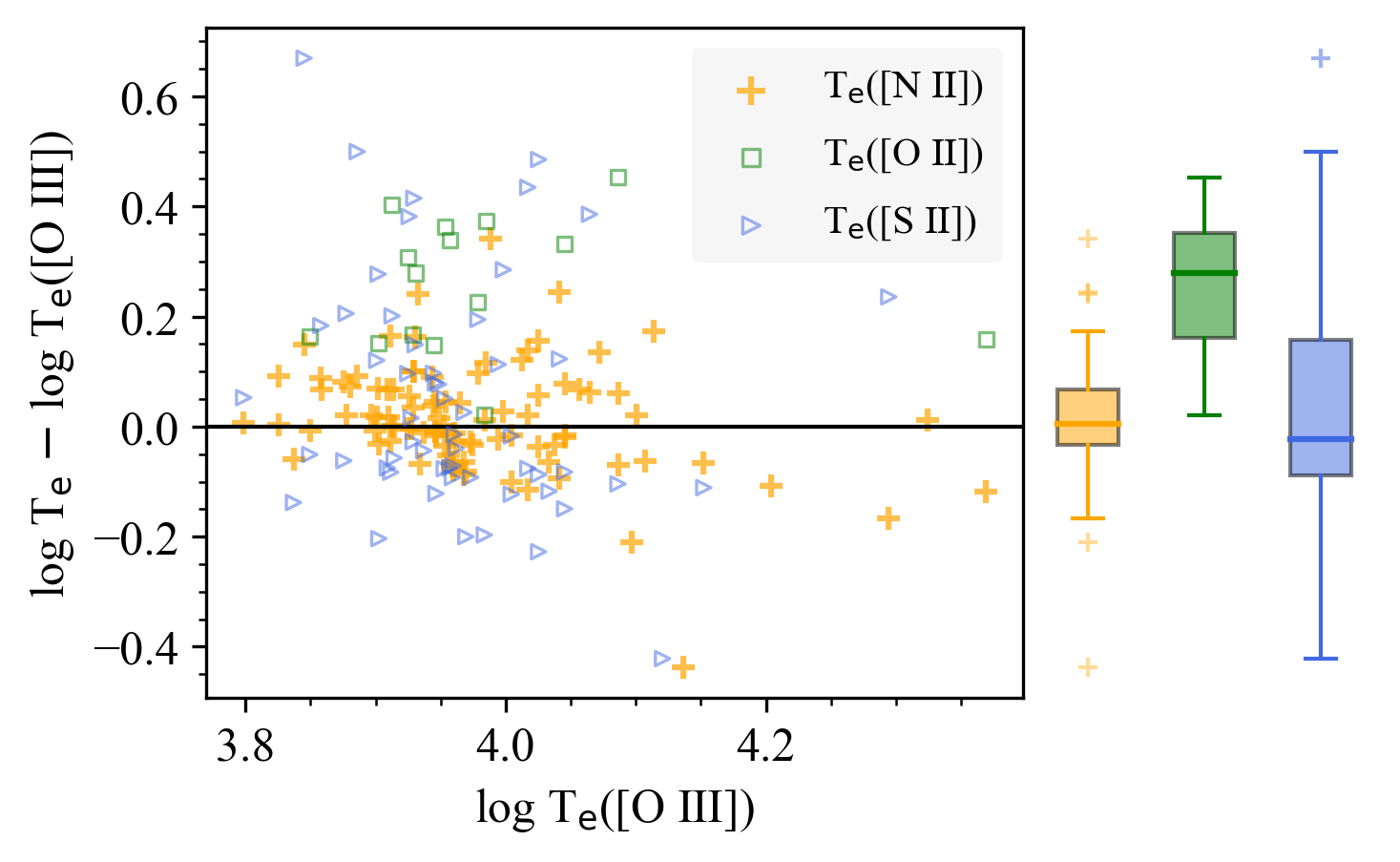
Figure 11: Comparison of electron temperature estimates using different diagnostic lines with those derived using [O iii] lines. Electron temperatures in the units of K are shown on a log scale, with values beyond the low or high limits excluded. The scatter plot displays the difference between electron temperature estimates using [N ii] (orange crosses), [O ii] (green squares) and [S ii] (blue triangles) compared to estimates from the [O iii] lines, plotted against electron temperature estimates using [O iii] lines. The box plots on the right show the distribution of the differences in electron temperature estimates, color-coded accordingly. The boxes depict the 25th to 75th percentiles, with the median indicated by a horizontal line. The whiskers extend to the 10th and 90th percentile, and outliers are represented by individual crosses.

Figure 10 displays a comparison of electron density estimates derived from different doublet lines with those obtained using [S ii] doublet lines, which serve as a reference due to their typical observational accessibility. The figure also showcases the distribution of differences between these estimates. Although there is a good overall agreement between the different emission-line diagnostics and the [S ii] lines within 0.05 dex, several outliers are observed above and below the 1:1 agreement line at 0, particularly for estimates using [Cl iii] and [Ar iv] lines. The discrepancies can be attributed to different sensitivity ranges of their line ratios, as illustrated in Fig. 2 in Méndez-Delgado et al. (2023). When compared to [S ii], both the [Cl iii] and [Ar iv] line ratios show limited sensitivity to $n_{\mathrm{e}}$ for $n_{\mathrm{e}}<1000$ cm^-3, resulting in an overestimation of $n_{\mathrm{e}}$ while they exhibit greater sensitivity at $n_{\mathrm{e}}>10,000\ \text{cm}^{-3}$, a range where [S ii] lines tend to underestimate $n_{\mathrm{e}}$.

The Pearson’s correlation coefficient is 0.48 between the low-ionization zone density diagnostics, $n_{\mathrm{e}}$([O ii]) and $n_{\mathrm{e}}$([S ii]), and a value of 0.64 between the medium-ionization zone diagnostics, $n_{\mathrm{e}}$([Ar iv]) and $n_{\mathrm{e}}$([Cl iii]). The median difference between $n_{\mathrm{e}}$([S ii]) and $n_{\mathrm{e}}$([O ii]) is $-$0.004 dex while at higher $n_{\mathrm{e}}$([S ii]) ($>7000$ cm^-3), $n_{\mathrm{e}}$([O ii]) is lower by 0.1-0.85 dex, resulting in a weak overall correlation. This discrepancy may be due to sensitivity limits of the line ratios as clearly demonstrated by Fig. 2 in Méndez-Delgado et al. (2023), their different dependence on electron temperatures or the atomic data, as discussed in Kisielius et al. (2009). The median difference between $n_{\mathrm{e}}$ derived from [Cl iii] and [Ar iv] lines is $-0.18$ dex, indicating a systematic difference. A typical uncertainty in $n_{\mathrm{e}}$([Cl iii]) and $n_{\mathrm{e}}$([Ar iv]) is around 0.12 dex. The discrepancy could be due to the measurement uncertainties, or it may indicate that power-law hydrogen density structures are not favoured, according to the photoionization models in Juan de Dios & Rodríguez (2021).

Figure 11 presents a comparison between electron temperatures obtained from different diagnostic lines, namely the [N ii], [O ii] and [S ii], and those derived from the [O iii] lines, which are usually reliably measured and not largely impacted by the recombination contributions. In our results, $T_{\mathrm{e}}$([N ii]) is lower than $T_{\mathrm{e}}$([O iii]) for 54% of the objects, with a median difference of 75 K between the two measures. The discrepancies are larger for higher values of $T_{\mathrm{e}}$ ($>13,000$ K). $T_{\mathrm{e}}$([O iii]) and $T_{\mathrm{e}}$([N ii]) exhibit moderate correlation with a coefficient of $r=0.59$. The dependence of the ratio $T_{\mathrm{e}}$([O iii])/$T_{\mathrm{e}}$([N ii]) on nebular excitation was examined in Kaler (1986), where a correlation between $T_{\mathrm{e}}$([O iii])/$T_{\mathrm{e}}$([N ii]) and the intensity of He ii $\lambda$4686 (which is only seen for high excitation PNe) was found. This correlation was later confirmed in KB94 and WL07 with Pearson’s correlation coefficients of $r=0.69$ and 0.70 respectively. Similarly, a correlation between $T_{\mathrm{e}}$([O iii])/$T_{\mathrm{e}}$([N ii]) and the nebular excitation class (EC) defined in Dopita & Meatheringham (1990) was found in Danehkar (2021) with $r=0.69$ for a sample of PNe surrounding Wolf–Rayet and weak-emission-line nuclei.

In our analysis, we exclude the object PNG 004.0-03.0, which was found to have a high temperature limit based on the [O iii] diagnostic lines, as observed in both our study and previous literature. We also excluded objects with weak line fluxes for [O iii] $\lambda$4363, He ii $\lambda$4686, and [N ii] $\lambda$5755, where F($\lambda$) $<10^{-16}\mathrm{erg~{}cm^{-2}s^{-1}}$. Despite these exclusions, we found that the correlations between $T_{\mathrm{e}}$([O iii])/$T_{\mathrm{e}}$([N ii]) and the intensity of He ii $\lambda$4686, as well as the excitation class (EC), were weak, with r-values of 0.54 and 0.31, respectively. We also evaluated the PN excitation class estimation scheme proposed by Reid & Parker (2010), which is expected to provide a better estimate of the central star effective temperatures, and used a linear interpolation for continuous estimates of the EC. The resulting r-value was 0.13. We suspect that the weaker correlation may be due to the overestimation of the recombination corrections of [N ii] $\lambda$5755 lines, which may have been contaminated by fluorescence, as suggested by previous studies (Escalante & Morisset, 2005; Escalante et al., 2012). When considering $T_{\mathrm{e}}$([N ii]) without recombination [O iii] $\lambda$4363 and [N ii] $\lambda$5755 emission contribution, the correlation coefficients became slightly stronger, with values of 0.69, 0.47, and 0.26, respectively. However, we should note that the weaker correction with EC in our data may be due to a larger range of $T_{\mathrm{e}}$([N ii]) in our study compared to the literature.

6.2 Elemental abundances determined for our sample PNe

The total elemental abundances of He, N, O, Ne, S, Ar, and Cl (relative to H) for each PN, along with their estimated uncertainties, are provided in Table.9. For all element except Ne, over 96% of the computed chemical abundances display uncertainties below 0.2 dex, and the median uncertainty is less than 0.05 dex. For Ne, 84% of the calculated abundances have uncertainties below 0.2 dex. PNe with an asterisk indicate those for which an abundance has been determined for the first time.

Table 9: Our measured PNe chemical abundances. Column 1 gives the PNG identification of the PN where an asterisk in front indicates the PN has an abundance determined for the first time; Column 2 is the logarithmic interstellar extinction ‘c’ at H$\beta$ derived from our spectra; Columns 3-9 give the determined abundances from the He/H, N/H, O/H, Ne/H, S/H, Ar/H, Cl/H ratios on a scale such that $\log$(H)$=12$. The ionic abundances for the sample objects are available online.

PN G	c(H$\beta$)	He/H	N/H	O/H	Ne/H	S/H	Ar/H	Cl/H
⋆000.1+02.6	2.14$\pm$0.08	11.14$\pm$0.01	8.34${}_{-0.07}^{+0.06}$	8.98${}_{-0.06}^{+0.05}$	8.46${}_{-0.07}^{+0.06}$	7.18${}_{-0.11}^{+0.10}$	6.76$\pm$0.05	4.84${}_{-0.13}^{+0.12}$
000.1+04.3	3.00$\pm$0.07	10.96$\pm$0.01	8.01${}_{-0.04}^{+0.03}$	8.55$\pm$0.03	7.99$\pm$0.03	6.73${}_{-0.06}^{+0.05}$	6.29${}_{-0.04}^{+0.03}$	5.01$\pm$0.04
000.1-02.3	1.54$\pm$0.06	11.07$\pm$0.01	8.28${}_{-0.04}^{+0.03}$	8.90$\pm$0.04	8.21$\pm$0.04	7.34$\pm$0.04	6.65$\pm$0.03	5.21${}_{-0.04}^{+0.03}$
000.2-01.9	1.58$\pm$0.08	10.93$\pm$0.02	8.12${}_{-0.04}^{+0.03}$	9.06${}_{-0.06}^{+0.05}$	8.61$\pm$0.05	7.02${}_{-0.07}^{+0.06}$	6.47${}_{-0.06}^{+0.05}$	5.07${}_{-0.07}^{+0.06}$
⋆000.2-04.6	1.44${}_{-0.06}^{+0.07}$	11.19$\pm$0.01	8.58${}_{-0.03}^{+0.02}$	9.01${}_{-0.05}^{+0.04}$	8.23$\pm$0.04	7.05${}_{-0.05}^{+0.04}$	6.61$\pm$0.04	5.14$\pm$0.03
⋆000.3+06.9	1.25$\pm$0.08	11.03$\pm$0.02	-	8.18$\pm$0.01	7.85$\pm$0.02	6.34$\pm$0.03	6.33$\pm$0.03	-
000.3-04.6	1.48$\pm$0.09	11.22$\pm$0.02	8.58$\pm$0.03	8.89${}_{-0.06}^{+0.05}$	8.13$\pm$0.04	6.99${}_{-0.07}^{+0.06}$	6.55${}_{-0.05}^{+0.04}$	5.26${}_{-0.04}^{+0.03}$
000.4-01.9	1.86$\pm$0.06	11.08${}_{-0.02}^{+0.01}$	8.40$\pm$0.04	8.86$\pm$0.04	8.00${}_{-0.05}^{+0.04}$	7.40${}_{-0.07}^{+0.06}$	6.83$\pm$0.05	5.57$\pm$0.04
000.4-02.9	1.03${}_{-0.08}^{+0.07}$	11.23$\pm$0.02	7.68${}_{-0.08}^{+0.07}$	8.74$\pm$0.04	8.16$\pm$0.03	6.26${}_{-0.16}^{+0.10}$	6.49$\pm$0.04	4.57$\pm$0.05
000.7+03.2	1.94$\pm$0.08	11.17$\pm$0.01	8.47${}_{-0.05}^{+0.04}$	9.03${}_{-0.08}^{+0.06}$	8.31$\pm$0.04	7.10${}_{-0.06}^{+0.05}$	6.81${}_{-0.04}^{+0.03}$	5.50$\pm$0.04
000.7-02.7	1.35$\pm$0.08	10.97$\pm$0.01	7.36${}_{-0.06}^{+0.05}$	8.43$\pm$0.04	7.74$\pm$0.03	6.04$\pm$0.06	5.78$\pm$0.03	4.47$\pm$0.04
⋆000.7-07.4	0.62$\pm$0.09	11.12$\pm$0.02	8.50${}_{-0.06}^{+0.05}$	8.75$\pm$0.05	8.26$\pm$0.04	7.18${}_{-0.09}^{+0.07}$	6.47$\pm$0.05	5.03$\pm$0.04
000.9-02.0	2.43$\pm$0.17	11.06$\pm$0.03	7.17${}_{-0.31}^{+0.18}$	8.64${}_{-0.37}^{+0.07}$	8.14${}_{-0.28}^{+0.05}$	6.66${}_{-0.16}^{+0.13}$	6.30${}_{-0.08}^{+0.06}$	5.01${}_{-0.09}^{+0.07}$
000.9-04.8	1.91$\pm$0.07	11.01$\pm$0.01	8.37${}_{-0.07}^{+0.06}$	9.03${}_{-0.05}^{+0.04}$	8.52$\pm$0.05	7.42${}_{-0.06}^{+0.05}$	6.70${}_{-0.04}^{+0.03}$	5.13${}_{-0.04}^{+0.03}$
⋆001.1-01.6	1.98$\pm$0.07	11.13$\pm$0.02	8.71$\pm$0.03	8.99${}_{-0.05}^{+0.04}$	8.39$\pm$0.03	7.11${}_{-0.06}^{+0.05}$	6.65$\pm$0.04	4.89${}_{-0.08}^{+0.07}$
001.2+02.1	2.56$\pm$0.07	11.00$\pm$0.02	7.99${}_{-0.06}^{+0.05}$	8.67$\pm$0.04	8.16$\pm$0.03	7.00$\pm$0.05	6.36$\pm$0.04	5.05${}_{-0.05}^{+0.04}$
⋆001.2-03.0	1.48$\pm$0.08	10.04${}_{-0.05}^{+0.03}$	8.39${}_{-0.06}^{+0.05}$	8.58${}_{-0.10}^{+0.08}$	-	6.91${}_{-0.06}^{+0.05}$	5.94$\pm$0.06	-
⋆001.3-01.2	2.89$\pm$0.07	11.09$\pm$0.01	8.42${}_{-0.06}^{+0.05}$	8.77${}_{-0.09}^{+0.07}$	-	6.99${}_{-0.13}^{+0.11}$	6.61${}_{-0.06}^{+0.05}$	5.56${}_{-0.07}^{+0.06}$
001.4+05.3	1.73$\pm$0.07	11.03$\pm$0.02	7.57${}_{-0.04}^{+0.03}$	8.70$\pm$0.05	7.82${}_{-0.06}^{+0.05}$	6.71${}_{-0.07}^{+0.06}$	6.24$\pm$0.05	5.02$\pm$0.05
001.6-01.3	3.38$\pm$0.11	11.09$\pm$0.02	8.58${}_{-0.07}^{+0.06}$	8.81${}_{-0.06}^{+0.04}$	8.18${}_{-0.08}^{+0.06}$	6.95${}_{-0.09}^{+0.07}$	6.47$\pm$0.05	5.43${}_{-0.13}^{+0.11}$
001.7+05.7	1.76$\pm$0.06	10.86${}_{-0.02}^{+0.01}$	7.43$\pm$0.06	8.19$\pm$0.04	7.42$\pm$0.03	6.11$\pm$0.05	5.71$\pm$0.03	4.33$\pm$0.04
001.7-04.4	0.65$\pm$0.07	10.62${}_{-0.03}^{+0.02}$	8.49$\pm$0.05	9.07${}_{-0.09}^{+0.08}$	-	6.95${}_{-0.05}^{+0.04}$	6.60${}_{-0.07}^{+0.06}$	5.34$\pm$0.05
002.0-06.2	0.43$\pm$0.03	11.00$\pm$0.02	7.95$\pm$0.05	8.72$\pm$0.04	8.06$\pm$0.03	6.93$\pm$0.05	6.42$\pm$0.07	4.94$\pm$0.04
002.1-02.2	1.56$\pm$0.08	10.96$\pm$0.02	7.79$\pm$0.04	8.56$\pm$0.03	7.92$\pm$0.02	6.68$\pm$0.04	6.10$\pm$0.04	4.93$\pm$0.04
002.1-04.2	1.48$\pm$0.07	10.91$\pm$0.02	7.42${}_{-0.05}^{+0.03}$	8.15${}_{-0.05}^{+0.03}$	7.55${}_{-0.04}^{+0.02}$	6.50${}_{-0.07}^{+0.05}$	5.96${}_{-0.05}^{+0.04}$	4.89${}_{-0.15}^{+0.06}$
002.2-09.4	0.36${}_{-0.04}^{+0.05}$	11.10$\pm$0.01	8.71${}_{-0.07}^{+0.06}$	8.75${}_{-0.04}^{+0.03}$	8.35$\pm$0.03	7.09${}_{-0.11}^{+0.10}$	6.66${}_{-0.04}^{+0.03}$	5.36$\pm$0.04
⋆002.3+02.2	2.69$\pm$0.07	11.20$\pm$0.02	8.34${}_{-0.06}^{+0.05}$	8.61${}_{-0.06}^{+0.05}$	8.26${}_{-0.12}^{+0.10}$	6.82${}_{-0.06}^{+0.05}$	6.34$\pm$0.04	4.51${}_{-0.06}^{+0.05}$
002.5-01.7	2.16$\pm$0.05	11.14$\pm$0.01	8.83$\pm$0.04	8.80$\pm$0.03	8.48${}_{-0.08}^{+0.07}$	7.30$\pm$0.05	6.73${}_{-0.04}^{+0.03}$	5.16${}_{-0.13}^{+0.12}$
⋆002.6+02.1	2.53$\pm$0.04	11.11$\pm$0.01	9.15$\pm$0.03	9.14${}_{-0.02}^{+0.01}$	8.68$\pm$0.02	7.63${}_{-0.06}^{+0.05}$	7.06${}_{-0.02}^{+0.01}$	5.27$\pm$0.04
002.7-04.8	1.05${}_{-0.07}^{+0.06}$	11.24$\pm$0.01	8.32${}_{-0.04}^{+0.03}$	8.53${}_{-0.04}^{+0.03}$	8.09$\pm$0.04	6.87$\pm$0.04	6.39${}_{-0.04}^{+0.03}$	5.06${}_{-0.04}^{+0.03}$
002.8+01.7	2.46$\pm$0.05	10.92$\pm$0.01	8.24${}_{-0.04}^{+0.03}$	8.64${}_{-0.05}^{+0.04}$	-	6.86${}_{-0.05}^{+0.04}$	6.47${}_{-0.05}^{+0.04}$	5.29${}_{-0.04}^{+0.03}$
⋆002.8+01.8	2.47$\pm$0.07	11.05$\pm$0.02	8.52$\pm$0.04	8.81$\pm$0.04	8.27${}_{-0.08}^{+0.06}$	7.25$\pm$0.04	6.52$\pm$0.04	4.00$\pm$0.06
002.9-03.9	1.13$\pm$0.05	11.03$\pm$0.01	7.94${}_{-0.16}^{+0.09}$	8.43$\pm$0.03	7.76$\pm$0.03	6.89${}_{-0.43}^{+0.15}$	6.13$\pm$0.03	4.96$\pm$0.04
003.2-06.2	0.62${}_{-0.08}^{+0.09}$	11.13$\pm$0.02	8.45${}_{-0.06}^{+0.05}$	8.70$\pm$0.04	8.20$\pm$0.04	7.00${}_{-0.14}^{+0.12}$	6.55${}_{-0.06}^{+0.05}$	5.30${}_{-0.05}^{+0.04}$
003.6-02.3	1.41${}_{-0.06}^{+0.05}$	11.18$\pm$0.01	8.47$\pm$0.04	8.68${}_{-0.04}^{+0.03}$	8.11$\pm$0.05	6.76${}_{-0.08}^{+0.07}$	6.49${}_{-0.05}^{+0.04}$	4.97$\pm$0.05
⋆003.7+07.9	2.56$\pm$0.03	10.91$\pm$0.01	9.43$\pm$0.03	9.00$\pm$0.01	8.86$\pm$0.04	7.49$\pm$0.03	6.60$\pm$0.02	-
003.7-04.6	0.81$\pm$0.10	10.94$\pm$0.02	8.42${}_{-0.11}^{+0.10}$	8.66${}_{-0.04}^{+0.03}$	8.05$\pm$0.02	7.07${}_{-0.08}^{+0.07}$	6.41$\pm$0.04	5.67$\pm$0.07
003.8-04.3	0.74$\pm$0.04	11.12$\pm$0.01	8.37${}_{-0.06}^{+0.05}$	8.76${}_{-0.05}^{+0.04}$	8.06${}_{-0.04}^{+0.03}$	6.96${}_{-0.06}^{+0.05}$	6.66$\pm$0.03	5.31${}_{-0.04}^{+0.03}$
003.9-02.3	1.86$\pm$0.05	11.16$\pm$0.01	8.42${}_{-0.03}^{+0.02}$	8.71$\pm$0.03	8.24$\pm$0.03	6.85${}_{-0.06}^{+0.05}$	6.59$\pm$0.04	5.24$\pm$0.03
003.9-03.1	1.32$\pm$0.05	10.99$\pm$0.01	7.99${}_{-0.06}^{+0.05}$	8.72$\pm$0.03	7.91$\pm$0.05	6.66$\pm$0.04	6.22$\pm$0.03	4.75$\pm$0.04
004.0-03.0	1.12$\pm$0.05	10.66$\pm$0.01	6.58$\pm$0.02	6.95$\pm$0.02	6.57$\pm$0.02	4.93$\pm$0.02	5.00${}_{-0.04}^{+0.03}$	3.52${}_{-0.07}^{+0.06}$
004.1-03.8	1.54${}_{-0.09}^{+0.08}$	11.02$\pm$0.02	7.88$\pm$0.04	8.41${}_{-0.04}^{+0.03}$	8.01$\pm$0.03	6.63${}_{-0.06}^{+0.05}$	6.05${}_{-0.05}^{+0.04}$	4.83${}_{-0.04}^{+0.03}$
004.2-03.2	1.55$\pm$0.13	11.02${}_{-0.03}^{+0.02}$	7.27${}_{-0.16}^{+0.11}$	8.43${}_{-0.05}^{+0.04}$	7.78$\pm$0.03	6.43${}_{-0.13}^{+0.09}$	5.94$\pm$0.05	4.75${}_{-0.08}^{+0.07}$
004.2-04.3	1.10${}_{-0.13}^{+0.14}$	11.01$\pm$0.03	8.07${}_{-0.06}^{+0.05}$	8.60$\pm$0.04	8.02$\pm$0.03	7.31${}_{-0.15}^{+0.11}$	6.11${}_{-0.07}^{+0.06}$	4.86${}_{-0.07}^{+0.06}$
⋆004.6+06.0	0.66$\pm$0.05	11.08$\pm$0.01	8.13${}_{-0.06}^{+0.05}$	8.78${}_{-0.06}^{+0.05}$	8.25${}_{-0.06}^{+0.05}$	6.95${}_{-0.10}^{+0.08}$	6.84$\pm$0.05	5.26$\pm$0.06
004.8+02.0	2.37$\pm$0.06	10.88$\pm$0.01	7.45${}_{-0.05}^{+0.04}$	8.33${}_{-0.07}^{+0.06}$	-	6.50${}_{-0.09}^{+0.08}$	6.00${}_{-0.06}^{+0.05}$	5.76${}_{-0.13}^{+0.10}$
004.8-05.0	0.78$\pm$0.05	11.15$\pm$0.01	8.03${}_{-0.08}^{+0.07}$	8.65${}_{-0.06}^{+0.05}$	8.29${}_{-0.06}^{+0.05}$	6.87${}_{-0.08}^{+0.07}$	6.50$\pm$0.04	5.05${}_{-0.04}^{+0.03}$
⋆005.0-03.9	1.22$\pm$0.07	11.16${}_{-0.09}^{+0.03}$	7.20${}_{-0.06}^{+0.05}$	7.41${}_{-0.05}^{+0.04}$	6.98${}_{-0.05}^{+0.04}$	5.84$\pm$0.06	5.54$\pm$0.05	3.43${}_{-0.13}^{+0.12}$
⋆005.2+05.6	1.01$\pm$0.04	11.14$\pm$0.01	8.18$\pm$0.05	8.61${}_{-0.05}^{+0.04}$	8.14${}_{-0.04}^{+0.03}$	6.83$\pm$0.05	6.52${}_{-0.04}^{+0.03}$	5.19${}_{-0.05}^{+0.08}$
⋆005.5+06.1	1.35$\pm$0.07	11.03$\pm$0.02	8.21${}_{-0.06}^{+0.05}$	8.70${}_{-0.11}^{+0.09}$	8.00${}_{-0.10}^{+0.08}$	6.63${}_{-0.05}^{+0.04}$	6.19${}_{-0.07}^{+0.06}$	5.29$\pm$0.06
⋆005.5-04.0	1.13$\pm$0.05	11.15$\pm$0.01	7.65$\pm$0.03	8.92${}_{-0.05}^{+0.04}$	-	7.21$\pm$0.05	6.77$\pm$0.03	5.65${}_{-0.06}^{+0.05}$
005.8-06.1	0.53$\pm$0.05	11.12$\pm$0.01	8.71$\pm$0.05	9.02$\pm$0.04	8.38$\pm$0.04	7.30$\pm$0.06	6.84${}_{-0.05}^{+0.04}$	5.48${}_{-0.04}^{+0.03}$
006.1+08.3	1.26$\pm$0.05	11.01$\pm$0.02	7.60$\pm$0.03	8.53$\pm$0.03	7.92$\pm$0.03	6.39${}_{-0.07}^{+0.06}$	5.98$\pm$0.04	4.76${}_{-0.04}^{+0.03}$
006.4+02.0	1.92${}_{-0.10}^{+0.09}$	11.12$\pm$0.02	8.54$\pm$0.03	8.95$\pm$0.03	8.40${}_{-0.03}^{+0.02}$	7.27${}_{-0.05}^{+0.04}$	6.80${}_{-0.05}^{+0.04}$	5.37$\pm$0.03
006.4-04.6	1.01$\pm$0.12	11.12$\pm$0.01	7.89${}_{-0.09}^{+0.07}$	8.62$\pm$0.04	-	6.86${}_{-0.07}^{+0.06}$	6.56$\pm$0.05	5.38${}_{-0.05}^{+0.06}$
006.8+02.3	2.14$\pm$0.08	11.03$\pm$0.01	7.87${}_{-0.05}^{+0.04}$	8.54${}_{-0.05}^{+0.04}$	7.79$\pm$0.03	6.46$\pm$0.05	5.92$\pm$0.04	4.85$\pm$0.04
006.8-03.4	1.41$\pm$0.02	10.90$\pm$0.01	7.35$\pm$0.02	8.29$\pm$0.02	7.65$\pm$0.01	6.13${}_{-0.06}^{+0.05}$	5.78$\pm$0.01	4.30$\pm$0.01

Table 10: continued

PN G	c(H$\beta$)	He/H	N/H	O/H	Ne/H	S/H	Ar/H	Cl/H
007.0+06.3	1.61$\pm$0.10	11.03$\pm$0.02	8.16${}_{-0.07}^{+0.06}$	8.73${}_{-0.05}^{+0.04}$	8.18$\pm$0.03	7.09${}_{-0.07}^{+0.06}$	6.61${}_{-0.06}^{+0.05}$	5.37${}_{-0.05}^{+0.06}$
007.0-06.8	0.72$\pm$0.08	11.13$\pm$0.02	8.28${}_{-0.07}^{+0.06}$	8.78${}_{-0.05}^{+0.04}$	8.23${}_{-0.05}^{+0.04}$	7.02${}_{-0.10}^{+0.08}$	6.58${}_{-0.06}^{+0.05}$	5.36${}_{-0.06}^{+0.05}$
⋆007.5+07.4	0.71${}_{-0.07}^{+0.06}$	11.16$\pm$0.01	8.28$\pm$0.03	8.81${}_{-0.05}^{+0.04}$	8.07$\pm$0.04	6.82$\pm$0.04	6.43${}_{-0.04}^{+0.03}$	5.10${}_{-0.04}^{+0.03}$
⋆007.6+06.9	1.03$\pm$0.04	11.14$\pm$0.01	7.92$\pm$0.03	8.49$\pm$0.03	7.94$\pm$0.02	6.53${}_{-0.06}^{+0.05}$	6.40$\pm$0.02	5.11$\pm$0.03
007.8-03.7	1.17${}_{-0.07}^{+0.06}$	11.14$\pm$0.01	8.35$\pm$0.03	8.77$\pm$0.04	8.05$\pm$0.03	7.08$\pm$0.10	6.43$\pm$0.03	5.52${}_{-0.06}^{+0.05}$
007.8-04.4	1.02$\pm$0.04	10.18${}_{-0.06}^{+0.02}$	8.34${}_{-0.06}^{+0.05}$	8.48${}_{-0.12}^{+0.09}$	-	6.66${}_{-0.08}^{+0.06}$	5.41$\pm$0.12	-
008.2+06.8	0.82$\pm$0.05	9.91$\pm$0.02	7.07${}_{-0.05}^{+0.04}$	7.67${}_{-0.06}^{+0.05}$	-	5.53${}_{-0.06}^{+0.04}$	5.08$\pm$0.04	3.86$\pm$0.04
008.4-03.6	1.49$\pm$0.06	10.99${}_{-0.06}^{+0.02}$	8.33${}_{-0.05}^{+0.04}$	9.01${}_{-0.11}^{+0.09}$	8.65${}_{-0.17}^{+0.13}$	6.90${}_{-0.05}^{+0.04}$	6.50${}_{-0.07}^{+0.06}$	4.90${}_{-0.09}^{+0.08}$
008.6-02.6	2.31$\pm$0.06	10.96$\pm$0.01	-	8.33$\pm$0.04	7.62$\pm$0.03	6.19${}_{-0.06}^{+0.05}$	5.77$\pm$0.03	4.58${}_{-0.04}^{+0.03}$
009.4-09.8	0.85$\pm$0.08	11.09$\pm$0.02	8.06${}_{-0.08}^{+0.06}$	8.64$\pm$0.04	8.14$\pm$0.03	6.83${}_{-0.06}^{+0.05}$	6.41$\pm$0.04	5.15$\pm$0.08
009.8-04.6	0.83$\pm$0.05	11.06$\pm$0.01	8.39${}_{-0.07}^{+0.06}$	8.87$\pm$0.04	8.32${}_{-0.05}^{+0.04}$	7.25${}_{-0.07}^{+0.06}$	6.68$\pm$0.04	5.45$\pm$0.05
351.1+04.8	1.15$\pm$0.06	11.05$\pm$0.02	8.14${}_{-0.04}^{+0.03}$	8.85$\pm$0.04	8.22$\pm$0.03	7.05${}_{-0.07}^{+0.06}$	6.62${}_{-0.05}^{+0.04}$	5.32${}_{-0.04}^{+0.03}$
351.2+05.2	1.00$\pm$0.05	10.97$\pm$0.01	8.51$\pm$0.03	8.78${}_{-0.06}^{+0.05}$	7.84${}_{-0.06}^{+0.05}$	6.58$\pm$0.04	6.19$\pm$0.05	5.03$\pm$0.04
351.6-06.2	0.70$\pm$0.05	11.15$\pm$0.01	8.68$\pm$0.03	8.88${}_{-0.04}^{+0.03}$	8.17$\pm$0.03	7.24${}_{-0.04}^{+0.03}$	6.83${}_{-0.03}^{+0.02}$	5.55$\pm$0.03
⋆351.9+09.0	0.51$\pm$0.05	11.02$\pm$0.01	7.29${}_{-0.14}^{+0.10}$	8.56$\pm$0.03	8.03$\pm$0.03	6.49${}_{-0.06}^{+0.05}$	6.11$\pm$0.02	4.90$\pm$0.04
351.9-01.9	2.93$\pm$0.05	11.04$\pm$0.01	8.24$\pm$0.02	8.66$\pm$0.02	8.20$\pm$0.01	6.92$\pm$0.04	6.35$\pm$0.03	5.36${}_{-0.03}^{+0.16}$
352.0-04.6	1.53$\pm$0.07	11.14$\pm$0.02	8.88${}_{-0.04}^{+0.03}$	9.02$\pm$0.04	8.42$\pm$0.04	7.30${}_{-0.06}^{+0.05}$	6.92${}_{-0.04}^{+0.03}$	5.43${}_{-0.04}^{+0.03}$
352.1+05.1	1.49${}_{-0.01}^{+0.02}$	11.10$\pm$0.01	8.56$\pm$0.02	8.76$\pm$0.01	8.32$\pm$0.01	7.01${}_{-0.05}^{+0.04}$	6.62$\pm$0.02	5.37$\pm$0.01
352.6+03.0	2.58$\pm$0.06	11.18$\pm$0.01	8.66$\pm$0.02	8.84$\pm$0.02	8.49$\pm$0.01	7.08$\pm$0.08	6.74${}_{-0.04}^{+0.03}$	5.50$\pm$0.02
⋆353.2-05.2	0.80$\pm$0.06	11.24$\pm$0.01	8.50${}_{-0.04}^{+0.03}$	8.69$\pm$0.03	8.09$\pm$0.05	6.64${}_{-0.06}^{+0.05}$	6.41${}_{-0.04}^{+0.03}$	4.47$\pm$0.05
353.3+06.3	0.91$\pm$0.05	10.96$\pm$0.02	7.72${}_{-0.09}^{+0.08}$	8.46${}_{-0.05}^{+0.04}$	7.94${}_{-0.08}^{+0.05}$	6.56${}_{-0.08}^{+0.07}$	6.00${}_{-0.05}^{+0.04}$	4.97${}_{-0.06}^{+0.05}$
353.7+06.3	0.81$\pm$0.07	11.05$\pm$0.02	8.10$\pm$0.05	8.81$\pm$0.04	8.02$\pm$0.10	6.88${}_{-0.06}^{+0.05}$	6.38$\pm$0.04	5.24$\pm$0.03
354.5+03.3	3.48$\pm$0.07	10.96$\pm$0.02	8.56$\pm$0.03	8.70$\pm$0.02	8.22$\pm$0.02	6.87$\pm$0.04	6.48$\pm$0.04	5.08${}_{-0.04}^{+0.03}$
354.9+03.5	2.33$\pm$0.07	11.08$\pm$0.01	8.23$\pm$0.05	8.62${}_{-0.07}^{+0.06}$	8.35${}_{-0.08}^{+0.07}$	6.90${}_{-0.09}^{+0.08}$	6.41${}_{-0.06}^{+0.05}$	5.15${}_{-0.05}^{+0.04}$
355.4-02.4	1.98$\pm$0.06	11.13$\pm$0.01	8.79$\pm$0.03	8.81$\pm$0.03	8.30$\pm$0.03	7.12$\pm$0.06	6.74${}_{-0.06}^{+0.05}$	5.45$\pm$0.03
355.9+03.6	1.47$\pm$0.07	10.71$\pm$0.02	7.13${}_{-0.14}^{+0.05}$	8.04${}_{-0.20}^{+0.07}$	7.60${}_{-0.20}^{+0.06}$	6.53${}_{-0.06}^{+0.05}$	5.68${}_{-0.07}^{+0.05}$	4.46${}_{-0.12}^{+0.07}$
355.9-04.2	1.19$\pm$0.03	11.17$\pm$0.02	8.58$\pm$0.02	9.11${}_{-0.15}^{+0.09}$	7.94${}_{-0.04}^{+0.03}$	7.39$\pm$0.11	6.85$\pm$0.05	5.76${}_{-0.04}^{+0.03}$
⋆356.1-03.3	1.20$\pm$0.05	11.14$\pm$0.01	8.55$\pm$0.02	8.90$\pm$0.04	8.20$\pm$0.04	7.00$\pm$0.04	6.57$\pm$0.04	5.50${}_{-0.06}^{+0.05}$
356.3-06.2	0.43$\pm$0.05	11.11$\pm$0.01	8.49${}_{-0.08}^{+0.05}$	8.70${}_{-0.07}^{+0.06}$	7.83${}_{-0.04}^{+0.03}$	6.84${}_{-0.06}^{+0.05}$	6.40${}_{-0.04}^{+0.03}$	5.07$\pm$0.04
⋆356.5-03.6	2.46$\pm$0.10	11.13$\pm$0.02	8.47${}_{-0.07}^{+0.06}$	8.78${}_{-0.05}^{+0.04}$	7.78${}_{-0.07}^{+0.06}$	7.05${}_{-0.07}^{+0.06}$	6.63${}_{-0.05}^{+0.04}$	5.44$\pm$0.04
⋆356.8+03.3	2.24$\pm$0.06	10.82$\pm$0.01	8.36$\pm$0.04	8.54${}_{-0.07}^{+0.06}$	-	6.65${}_{-0.11}^{+0.10}$	6.39${}_{-0.06}^{+0.05}$	5.45$\pm$0.08
356.8-05.4	0.84$\pm$0.06	11.12$\pm$0.01	8.14$\pm$0.03	8.86$\pm$0.04	7.87$\pm$0.04	6.84$\pm$0.04	6.49${}_{-0.04}^{+0.03}$	5.03$\pm$0.03
356.9+04.4	1.94$\pm$0.05	10.94$\pm$0.01	8.44${}_{-0.06}^{+0.05}$	8.67${}_{-0.06}^{+0.05}$	8.01${}_{-0.04}^{+0.03}$	6.99${}_{-0.07}^{+0.06}$	6.55$\pm$0.04	5.07$\pm$0.04
357.0+02.4	2.32$\pm$0.06	11.12$\pm$0.01	8.55${}_{-0.04}^{+0.03}$	8.88$\pm$0.03	8.23$\pm$0.04	7.23$\pm$0.06	6.78${}_{-0.04}^{+0.03}$	5.55${}_{-0.05}^{+0.04}$
357.1+03.6	0.99$\pm$0.05	11.00$\pm$0.01	8.06${}_{-0.05}^{+0.04}$	8.73$\pm$0.04	8.40$\pm$0.04	7.17${}_{-0.07}^{+0.06}$	6.58$\pm$0.04	5.03${}_{-0.06}^{+0.05}$
⋆357.1+04.4	1.81${}_{-0.05}^{+0.06}$	11.16$\pm$0.01	7.36${}_{-0.09}^{+0.07}$	9.03${}_{-0.08}^{+0.07}$	8.51${}_{-0.11}^{+0.08}$	6.69${}_{-0.15}^{+0.10}$	6.54${}_{-0.07}^{+0.06}$	4.90${}_{-0.07}^{+0.06}$
357.1-04.7	1.02${}_{-0.05}^{+0.04}$	10.21$\pm$0.02	8.50${}_{-0.08}^{+0.06}$	8.50${}_{-0.17}^{+0.11}$	-	6.86${}_{-0.08}^{+0.07}$	-	5.64${}_{-0.10}^{+0.07}$
⋆357.2+02.0	2.34$\pm$0.07	10.98$\pm$0.01	7.87$\pm$0.04	8.83$\pm$0.04	8.16$\pm$0.03	6.65$\pm$0.05	6.30$\pm$0.03	4.88$\pm$0.04
⋆357.3+04.0	1.65$\pm$0.05	11.05$\pm$0.01	8.18${}_{-0.07}^{+0.06}$	8.81$\pm$0.03	8.26$\pm$0.03	7.05${}_{-0.07}^{+0.06}$	6.55$\pm$0.03	4.98${}_{-0.04}^{+0.03}$
⋆357.5+03.1	1.98$\pm$0.07	-	6.98${}_{-0.08}^{+0.07}$	7.09${}_{-0.20}^{+0.13}$	-	5.94${}_{-0.07}^{+0.06}$	-	4.89${}_{-0.14}^{+0.11}$
357.5+03.2	2.30$\pm$0.08	11.11$\pm$0.01	8.86$\pm$0.05	8.93$\pm$0.04	8.47${}_{-0.06}^{+0.05}$	7.37${}_{-0.06}^{+0.05}$	6.78${}_{-0.05}^{+0.04}$	5.43${}_{-0.08}^{+0.07}$
357.6-03.3	1.59$\pm$0.06	11.16$\pm$0.01	7.95${}_{-0.05}^{+0.04}$	8.53${}_{-0.11}^{+0.09}$	8.43${}_{-0.17}^{+0.12}$	6.51$\pm$0.04	6.09${}_{-0.07}^{+0.06}$	-
⋆357.9-03.8	1.56$\pm$0.05	11.25$\pm$0.01	6.78${}_{-0.10}^{+0.08}$	7.63$\pm$0.04	7.27$\pm$0.04	5.31${}_{-0.07}^{+0.06}$	5.82$\pm$0.04	3.96${}_{-0.05}^{+0.04}$
357.9-05.1	1.32$\pm$0.07	11.07$\pm$0.01	8.61${}_{-0.03}^{+0.02}$	8.78$\pm$0.04	8.23$\pm$0.03	6.97${}_{-0.04}^{+0.03}$	6.47$\pm$0.03	5.16$\pm$0.03
⋆358.0+09.3	0.63${}_{-0.11}^{+0.12}$	11.11$\pm$0.02	7.40${}_{-0.10}^{+0.08}$	8.51${}_{-0.05}^{+0.04}$	7.94$\pm$0.04	6.11${}_{-0.07}^{+0.06}$	6.12${}_{-0.05}^{+0.04}$	4.63${}_{-0.08}^{+0.07}$
358.2+03.5	2.69${}_{-0.11}^{+0.10}$	10.96$\pm$0.02	7.91${}_{-0.07}^{+0.06}$	8.47${}_{-0.06}^{+0.05}$	7.61$\pm$0.04	6.56${}_{-0.09}^{+0.07}$	5.97${}_{-0.05}^{+0.04}$	4.85$\pm$0.05
358.2+04.2	2.15$\pm$0.06	11.09$\pm$0.01	8.26${}_{-0.04}^{+0.03}$	8.75$\pm$0.03	8.32$\pm$0.03	6.95${}_{-0.10}^{+0.09}$	6.65${}_{-0.04}^{+0.03}$	5.40$\pm$0.04
⋆358.5+02.9	2.09$\pm$0.06	10.95$\pm$0.02	7.34${}_{-0.04}^{+0.03}$	8.37$\pm$0.04	7.78$\pm$0.03	6.31${}_{-0.06}^{+0.05}$	5.85$\pm$0.03	4.57$\pm$0.04
358.5-04.2	1.52$\pm$0.05	10.96$\pm$0.03	7.66$\pm$0.04	8.34${}_{-0.04}^{+0.03}$	7.75${}_{-0.04}^{+0.03}$	6.77${}_{-0.06}^{+0.05}$	6.15${}_{-0.04}^{+0.03}$	4.81${}_{-0.04}^{+0.03}$
⋆358.6+07.8	0.98$\pm$0.05	11.04$\pm$0.01	8.07$\pm$0.04	8.72$\pm$0.03	8.13${}_{-0.03}^{+0.02}$	7.09$\pm$0.05	6.36$\pm$0.03	5.42${}_{-0.04}^{+0.03}$
358.6-05.5	0.80$\pm$0.06	11.18$\pm$0.01	8.40${}_{-0.04}^{+0.03}$	8.51${}_{-0.03}^{+0.02}$	8.01$\pm$0.03	6.71${}_{-0.07}^{+0.06}$	6.39$\pm$0.04	4.73$\pm$0.06
358.7+05.2	2.57$\pm$0.10	10.26$\pm$0.02	8.32${}_{-0.06}^{+0.05}$	8.51${}_{-0.11}^{+0.09}$	-	6.90${}_{-0.08}^{+0.06}$	6.28${}_{-0.08}^{+0.07}$	5.96${}_{-0.18}^{+0.15}$
358.8+03.0	1.89$\pm$0.06	11.11$\pm$0.01	8.45$\pm$0.03	8.88$\pm$0.03	8.19$\pm$0.03	7.14$\pm$0.04	6.71$\pm$0.03	5.25${}_{-0.04}^{+0.03}$
358.9+03.4	2.54$\pm$0.07	11.11$\pm$0.01	8.83$\pm$0.02	8.91$\pm$0.02	8.48$\pm$0.02	7.57${}_{-0.06}^{+0.05}$	6.97${}_{-0.04}^{+0.03}$	5.77${}_{-0.02}^{+0.03}$
359.0-04.1	1.16$\pm$0.07	11.14$\pm$0.01	8.71$\pm$0.03	8.88$\pm$0.04	8.31${}_{-0.05}^{+0.04}$	7.14$\pm$0.05	6.69$\pm$0.04	5.25${}_{-0.04}^{+0.03}$
359.1-02.9	1.31$\pm$0.06	11.13$\pm$0.01	8.73${}_{-0.04}^{+0.03}$	8.85$\pm$0.04	8.24${}_{-0.05}^{+0.04}$	6.85${}_{-0.08}^{+0.06}$	6.54$\pm$0.04	5.26${}_{-0.10}^{+0.09}$
⋆359.2+04.7	2.10$\pm$0.07	11.24$\pm$0.02	7.43${}_{-0.09}^{+0.05}$	8.28${}_{-0.12}^{+0.07}$	-	5.87${}_{-0.17}^{+0.08}$	6.43${}_{-0.08}^{+0.05}$	5.54${}_{-0.07}^{+0.05}$
359.3-01.8	3.28$\pm$0.05	10.20$\pm$0.02	8.30${}_{-0.12}^{+0.09}$	8.54${}_{-0.21}^{+0.13}$	-	6.95${}_{-0.15}^{+0.09}$	5.99${}_{-0.09}^{+0.08}$	5.64${}_{-0.18}^{+0.11}$
359.6-04.8	0.95$\pm$0.04	11.28$\pm$0.01	7.33$\pm$0.06	8.13$\pm$0.03	7.65$\pm$0.03	6.35${}_{-0.07}^{+0.06}$	6.13$\pm$0.03	4.64${}_{-0.05}^{+0.04}$

Table 11: continued

PN G	c(H$\beta$)	He/H	N/H	O/H	Ne/H	S/H	Ar/H	Cl/H
359.7-01.8	2.47$\pm$0.13	10.97$\pm$0.02	7.47${}_{-0.43}^{+0.17}$	8.59${}_{-0.43}^{+0.09}$	7.48${}_{-0.05}^{+0.04}$	6.40${}_{-0.43}^{+0.13}$	6.06${}_{-0.05}^{+0.04}$	4.84${}_{-0.07}^{+0.06}$
⋆359.8+02.4	2.85$\pm$0.08	10.79$\pm$0.01	8.44${}_{-0.05}^{+0.04}$	8.78${}_{-0.07}^{+0.06}$	-	6.96${}_{-0.08}^{+0.07}$	6.43${}_{-0.07}^{+0.06}$	5.51${}_{-0.06}^{+0.05}$
359.8+03.7	2.32$\pm$0.09	10.98$\pm$0.02	7.63${}_{-0.07}^{+0.06}$	8.53${}_{-0.06}^{+0.05}$	-	6.63${}_{-0.08}^{+0.07}$	6.16${}_{-0.06}^{+0.05}$	5.08${}_{-0.06}^{+0.05}$
⋆359.8+05.2	1.33$\pm$0.04	11.03$\pm$0.01	7.99${}_{-0.05}^{+0.04}$	8.37${}_{-0.12}^{+0.09}$	-	6.72$\pm$0.04	6.07${}_{-0.06}^{+0.05}$	6.20${}_{-0.13}^{+0.11}$
359.8+05.6	0.72${}_{-0.08}^{+0.07}$	10.11$\pm$0.03	8.26${}_{-0.09}^{+0.07}$	8.66${}_{-0.17}^{+0.11}$	-	7.03${}_{-0.15}^{+0.11}$	6.45${}_{-0.09}^{+0.07}$	5.86${}_{-0.14}^{+0.11}$
359.8+06.9	1.42${}_{-0.07}^{+0.06}$	11.02$\pm$0.02	8.57$\pm$0.04	8.78${}_{-0.03}^{+0.02}$	8.23$\pm$0.03	7.02${}_{-0.05}^{+0.04}$	6.48$\pm$0.04	5.15$\pm$0.03
359.8-07.2	0.67${}_{-0.09}^{+0.10}$	10.95$\pm$0.02	7.48${}_{-0.09}^{+0.07}$	8.44$\pm$0.03	7.83$\pm$0.02	6.27$\pm$0.05	5.88$\pm$0.03	5.05${}_{-0.07}^{+0.06}$
359.9-04.5	1.97${}_{-0.10}^{+0.09}$	11.16$\pm$0.02	8.76$\pm$0.03	8.78$\pm$0.03	8.36$\pm$0.02	7.21${}_{-0.09}^{+0.08}$	6.78${}_{-0.05}^{+0.04}$	5.55${}_{-0.04}^{+0.15}$

We compared our data with results of PNe in the Galactic bulge given in Chiappini et al. (2009) CGS09, which combined the data sets from Górny et al. (2004) which is itself a merger of PNe abundance measures from Cuisinier et al. (1999), Escudero & Costa (2001), and Escudero et al. (2004), Górny et al. (2009) and Wang & Liu (2007). We limited our comparison to high-quality measurements with reported uncertainties of less than 0.3 dex (removing of 25% of their data set), as done in their analysis. The median, 25th and 75th percentile values of He/H, N/H, O/H, Ar/H, Ne/H, S/H, Cl/H derived in this work and in CGS09 are presented in Table.12 together with the number of PNe with each measurement available.

Table 12: Statistics of chemical abundances for all the Bulge PNe measured in this work and in CGS09. Columns 2-5 provide information about the median, 25th and 75th percentile values (in parentheses in columns 2-3), and the number of PNe measurements used for the calculation (in brackets in column 5). Columns 6-9 present results obtained from the combined literature data sets in CGS09, expressed in the same manner. Column 10 displays solar abundances taken from Asplund et al. (2009). The abundances are given on a log scale where $\log$(H)$=12$

	This work				CGS09			Sun
He/H	11.06	[10.97, 11.14]	(123)		11.11	[11.05, 11.19]	(144)	10.93$\pm$0.01
N/H	8.27	[7.88, 8.49]	(122)		8.11	[7.76, 8.50]	(123)	7.83$\pm$0.05
O/H	8.70	[8.53, 8.83]	(124)		8.57	[8.40, 8.72]	(117)	8.69$\pm$0.05
Ne/H	8.14	[7.92, 8.29]	(105)		7.93	[7.71, 8.17]	(77)	7.93$\pm$0.10
S/H	6.90	[6.63, 7.08]	(124)		6.79	[6.54, 7.04]	(94)	7.12$\pm$0.03
Ar/H	6.44	[6.14, 6.61]	(122)		6.34	[6.05, 6.56]	(120)	6.40$\pm$0.13
Cl/H	5.14	[4.89, 5.41]	(119)		6.22	[6.00, 6.50]	(47)	5.50$\pm$0.30

In comparison to the CGS09 findings, our results show higher median abundances for N and the alpha elements (O, Ne, S, and Ar), with differences ranging from 0.10-0.30 dex. Notably, the median O/H, Ne/H, Ar/H values in our data are slightly super-solar. However, the median abundance for S, other $\alpha$ elements, remains sub-solar due to the well-known ’sulphur anomaly’ (Henry et al., 2004, 2012). Our results also show a slightly lower median abundance for He, with a tail towards lower values, by approximately 0.05 dex. In terms of chlorine, our median abundance value is lower than the literature value by 1.09 dex. This discrepancy is primarily due to the CGS09 study, where most of the Cl/H values are derived from GCS09. We discuss the reasons for this discrepancy in Section 5.1. The Cl/H results in CGS09 are mostly extremely super-solar, which is also contrary to the behaviour of other alpha elements in their results. In contrast, 90% of the Cl/H values in our results are sub-solar, and the difference between the PN Cl abundances and solar abundance becomes smaller. Thus, we believe that our Cl/H estimation is more reliable.

In summary, our data offers a highly accurate and precise representation of the general abundance pattern of PNe in the Galactic bulge, thanks to the consistently reduced and analysed high s/n VLT spectra, the availability of emission lines for a broader range of ionic species, and the incorporation of updated atomic data and the ICF scheme introduced in DMS14. Our results reveal a systematic increase in median values for elemental abundances across the majority of elements. The median abundances of alpha elements, O, Ne, and Ar, are found to be super-solar in our assessment.

7 Discussion

It is clear from this work that accurate PN physical conditions and abundance measures, even determined from excellent, high quality s/n spectra is an inherently difficult process as is the comparison with previous work. There are many reasons for this. Prime among these is the assumption that chemical abundances determined for any individual PN are representative of the entire nebula whereas we know that internal abundance variations do exist, albeit with small variations (e.g., Manchado et al. (1988); Danehkar et al. (2013)). Nevertheless, for the comparisons made here we use a single, overall abundance estimate as measured from an integrated 1-D spectrum from our compact PNe that are all $\leq$10 arcseconds across. Hence decent central, representative fractions of all our PNe are always sampled by the spectrograph slit. We also know that PNe are complex, resolved 3-D objects with internal condensations, density, temperature and ionisation variations etc, e.g. Monteiro et al. (2004); Akras et al. (2016). An important secondary factor, especially when comparing with other work, are issues such as the chosen telescope and spectrograph, the slit widths and positions in terms of orientation on the projected PN image and offsets from any CSPN and of course the observing conditions (seeing, transparency, airmass etc.) all of which vary between data sets.

The future of PNe abundance determinations is with deep IFU work such as in Danehkar et al. (2013); García-Rojas et al. (2022). IFUs have already shown how physical conditions and chemical abundances can vary across a given PN. However, until direct point-to-point mapping of physical parameters and chemical abundances based on IFU observations are available for large samples of PNe from different studies, this type of research remains essential. Nevertheless, the currently best plasma diagnostics used to determine the same property for some individual PNe do not show the levels of agreement hoped for and for all the reasons given above. Nevertheless, we believe we have produced the most internally self-consistent and robust data set to date for PNe abundance studies.

7.1 Correlations between the abundances $\alpha$-element

The $\alpha$-elements, including O, Ne, S, and Ar, are produced via the alpha processes during the evolution of massive stars, where nuclear fusion transforms helium into elements heavier than carbon. As these elements share common synthesis sites in massive stars (e.g. Henry et al., 2008; Esteban et al., 2020), their elemental abundances are expected to vary in lockstep. Therefore, in low- to- intermediate-mass stars, including the PN progenitors, their abundance ratios should remain constant. Similarly, Cl is produced by single particle (proton or neutron) capture by an S or Ar isotope, and therefore, indicating that it should exhibit similar behaviour (Esteban et al., 2015). Thus, generally, the abundances of alpha elements observed in PNe reflect the amounts that were initially present in the star-forming gas of the progenitor star, which enables PNe to serve as a tool for establishing the metallicity of the ISM during the formation of PN progenitor stars (Kwitter & Henry, 2022).

Among these elements, O is commonly used as a proxy for metallicity in ionised gases around stars, and a lockstep behaviour between $\alpha$ elements has been demonstrated in H ii regions and blue compact galaxies (BCG), with a strong correlation between elemental abundances of Ne, Ar and S, and O/H and a slope close to unity on a log scale. However, previous studies on PN have observed a slightly weaker correlation. To investigate the lockstep behaviour with PN abundances compiled in this work, we compared the abundances of $\alpha$-elements Ne and Ar, along with Cl, with that of oxygen in Fig. 12. The plot showing the relationship between S/H and O/H will be presented in the next paper in the series (Tan & Parker, submitted), where we specifically address the well-known ‘sulfur anomaly’ observed in PNe. Thus, it is not included in the current paper.

Each element-versus-oxygen plot was fitted with a straight line using the least squares fitting method. The slopes, intercepts of best-fit lines, and correlation coefficients are summarised in Table 13. For Ne and Ar, the dashed line represents the best-fit to a collection of published H ii region and BCG abundances (H2BCG) that clearly demonstrating the lockstep behaviour of $\alpha$ elements, with abundances of H ii regions from Kennicutt Jr et al. (2003) and BCGs compiled by Izotov & Thuan (1999). The analogous fit for Cl was inferred from a study of Galactic disk H ii regions by Arellano-Córdova et al. (2020). The red asterisks in the figure denote solar abundances.

Previous studies on PN abundances (Henry et al., 2004; Milingo et al., 2010, e.g.) have observed the lockstep behaviour with correlation coefficients of around 0.7 of Ne and Ar with a slope around 0.9 (Kwitter & Henry, 2022). However, this study obtained a much stronger correlation than those in the literature of around 0.85. The best-fit line for Ar/h versus O/H is highly consistent with the H2BCG results, suggesting that the previous less apparent lockstep behaviour observed in PNe could largely be attributed to observational and measurement errors. However, the Ne/H results from PNe do not agree with the best-fit of H2BCG results at extremely sub-solar abundances, which could be due to uncertainties in ICFs used to account for unobserved ionization stages more dominant than Ne²⁺. As a result, the slope derived for Ne/H versus O/H is smaller than unity.

As previously mentioned in Sec. 9, the determination of Cl/H is typically subject to uncertainty. The Cl/H versus O/H plot appears messier, exhibiting large scatters and increased measurement uncertainty at extremely sub-solar and super-solar abundances. Among all elements, the correlation between Cl/H and O/H is the weakest, with a correlation coefficient of $r=0.59$.

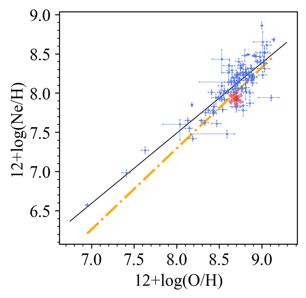
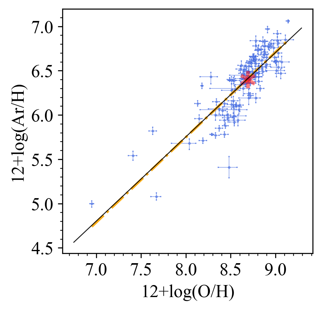
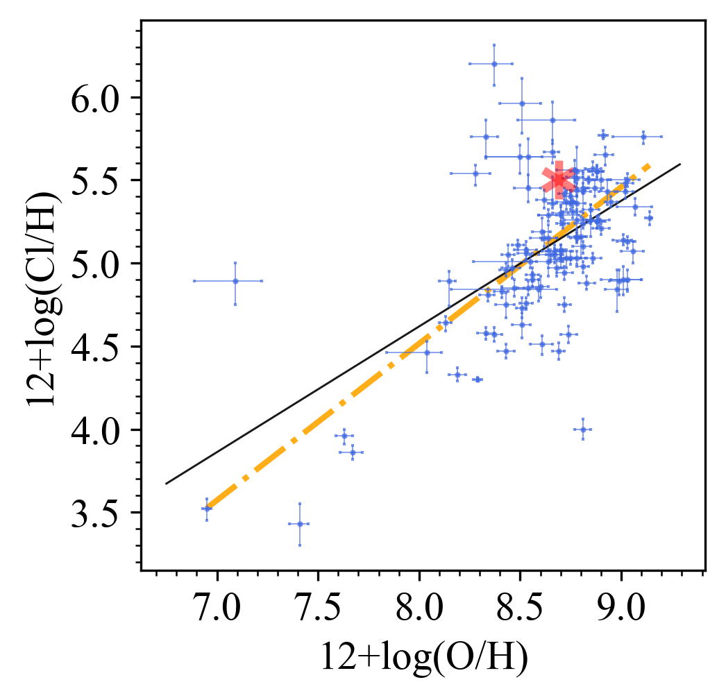
Figure 12: Abundances for $\log$(Ne/H), $\log$(Ar/H) and $\log$(Cl/H) for all PNe in our sample that provide an estimate plotted against $\log$(O/H), with error bars are from our measurement uncertainties. The black solid line in each panel represents the best-fit to the data. The best-fit parameters and associated uncertainties are presented in Table.13. For Ne and Ar, the dashed orange lines show the fit to abundances for H ii regions and BCGs from the literature. The orange dashed line for Cl presents an analogous fit based on abundances of Galactic disk H ii regions from Arellano-Córdova et al. (2020). The red asterisks denote the solar abundances.

X/H vs. O/H	Slope	y-Intercept	r	# of PNe
Ne	$0.90\pm 0.05$	$\ \ 0.32\pm 0.46$	0.86	105
Ar	$0.95\pm 0.06$	$-1.86\pm 0.48$	0.84	122
Cl	$0.76\pm 0.10$	$-1.44\pm 0.83$	0.59	119

Table 13: Least squares fit parameters and Pearson’s r values for $\alpha$-element correlations. The straight line was fit to $12+\log$(O/H) and $12+\log$(X/H). The number of PNe used is shown in the last column.

To conclude, the expected lockstep behaviour for alpha elements is more prominent in our data compared to previous PN abundance studies. We observe a strong correlation between O/H and both Ar/H and Ne/H on a log scale, as reported in the literature. The lockstep association between Cl and O is not clearly evident in our data, which we attribute to large measurement uncertainties.

7.2 He and N abundances

He and N are elements that could be produced in more massive PN progenitors as suggested by Kaler (1978) and Kaler & Jacoby (1990). We find 104 out of 124 PNe exhibit He/H measurements greater than solar (i.e. $>10.93$) while with several objects with measured $12+\log$(He/H) lower than 10.3. The derived N enrichment, $\log$(N/O), range from $-1.67$ to 0.43, with a median value of $-0.48_{-0.37}^{+0.29}$ dex. This is 0.09 and 0.15 dex lower than the results compiled in KB94 for southern PNe and in CGS09 for the bulge PNe, respectively. We remark there that the KB94 ICF scheme we adopted for N abundance in this study uses N/O$=$N⁺/O⁺ and we observe large discrepancies in N/H when comparing with the literature. This discrepancy could be due to the subtraction of the recombination contribution of [N ii] and [O ii] auroral lines. In this case, ignoring the recombination correction could lead to significant systematic uncertainties.

Fig. 13 presents the relationship between N/O and He/H for all objects with measurable abundances. A significant fractions of objects in our sample exhibit N enrichment above the solar value. In addition to a few objects show extremely sub-solar He/H values, which are presumably underestimated, as well as a few objects with low N/O ratios in which the large uncertainties might present as discussed in Wesson et al. (2018), the overall pattern suggests that high N/O values are associated with high He/H. We will further use the measurements of N enrichment and He/H to investigate the central star properties of PNe in Paper V in this series of papers.

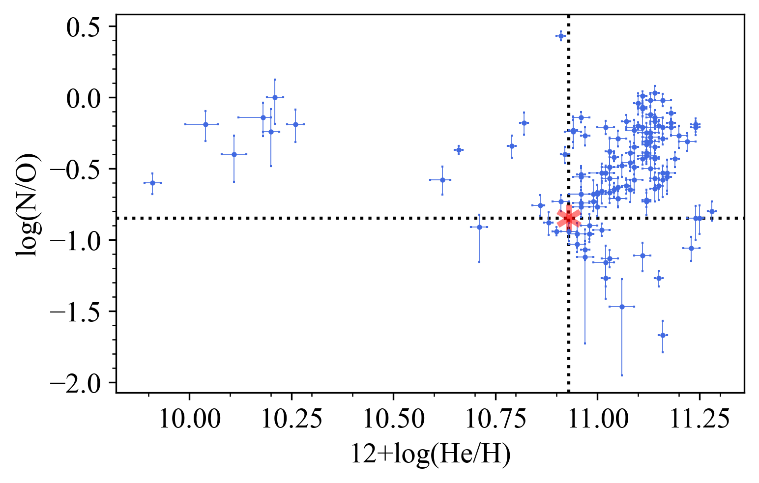
Figure 13: The N enrichment relative to O, $\log$(N/O), versus the he abundances $12+\log$(He/H), of 121 PNe in this sample. The horizontal black dotted line indicates the solar $12+\log$(He/H) values of 10.93 while the vertical line represents the solar nitrogen enrichment of $-0.85$. The red asterisks also denote the solar values.

7.3 Oxygen-poor PNe in this bulge sample

Three PNe, PNG 004.0-03.0, PNG 005.0-03.9 and PNG 357.5+03.1 are measured with extremely sub-solar oxygen abundances, with $12+\log$(O/H) $<7.5$ dex ( 15.5 times lower than the solar abundance). Their $12+\log$(O/H) estimates are $6.95\pm 0.02$, $7.41^{+0.04}_{-0.05}$ and $7.09^{+0.13}_{-0.20}$ dex, respectively. Despite large uncertainties in O/H for PNG 357.5+03.1, where the lower error is 46%, the O/H values measured for PNG 004.0-03.0 and PNG 005.0-03.9 have good precision, with uncertainties below 0.1 dex, confirming their oxygen poor status based on our spectroscopic observations. The extremely sub-solar oxygen abundance of PNG 004.0-03.0 has been noticed in previous studies, such as Peña et al. (1991) and Exter et al. (2004). Torres-Peimbert et al. (1997) and Miszalski et al. (2009) found that this anomalously low abundance is primarily due to low spatial resolution ground-based observations averaging over the strong spatial variation of [O iii $\lambda$4363/$\lambda$5007. Torres-Peimbert et al. (1997) measured an $12+\log$(O/H) value of 8.5 dex from HST spectroscopy of the inner nebula, while Miszalski et al. (2011) calculated an $12+\log$(O/H) of 8.3 dex in the outer nebula using VLT/FLAMES IFU observations. PNG 005.0-03.9 has a complex structure classified as Eamrs according to Tan et al. (2023a), all the temperature diagnostic lines, including [O ii], [N ii] and [O iii], give an estimate of electron temperatures greater than 15,000 K, which is similar to PNG 004.0-03.0. The low oxygen abundance measured with the VLT spectroscopy could be due to the low spatial resolution as for PNG 004.0-03.0.

PNG 357.5+03.1 is a very compact and low-excitation nebula with no [O iii] $\lambda$4363 line detected in its spectra. Only the weak [O iii] $\lambda$5007 lines of O²⁺ were well-detected with low s/n.

8 Conclusions

We have presented logarithmic extinction coefficients, plasma diagnostics of $n_{\mathrm{e}}$ and $T_{\mathrm{e}}$ and elemental abundances of He, N, O, Ne, S, Ar and Cl for a well-defined sample of 124 Galactic bulge PNe with high-quality, wide-wavelength coverage optical spectra obtained using the ESO VLT/FORS2 with consistent instrumental configurations and observing strategies. We believe this represents the most self-consistent and well characterised sample of PNe available with high s/n spectra, from which well-determined abundances are compiled. For 34 PNe, the abundance determinations are presented for the first time, significantly adding ($\sim 14$%) to the Bulge PNe population abundances. Moreover, for an additional 6 Bulge PNe, we provide the first reliable abundances. Comparing our work with the best previous Bulge PNe abundances in the literature for PNe overlapping with our sample demonstrates the robustness and overall reliability and consistency of this sample.

The physical parameters in PNe exhibit a wider range in this study. The low-to-medium resolution spectroscopic observation from the VLT exhibit excellent consistency with previous high-resolution spectra with 2-m class telescope, demonstrating the reliability of weak line detection, the line deblending methods and our line flux measurement, particularly for weak recombination lines. Our abundance compilation, which adopted updated atomic data and ICF schemes introduced in DMS14, results in overall higher abundances of alpha elements than solar compared to the general abundance pattern in the literature. The lockstep behaviour of alpha elements, which was less evident in previous studies, is clearly observed in our results.

The further analysis and investigation of these abundances form the basis of the following paper in the series.

Data Availability

The raw VLT/FORS2 spectroscopic data can be accessed through the ESO archive facility at http://archive.eso.org/. The codes for the analysis, as well as intermediate data products are available from ST under reasonable request.

References

- Acker et al. (1991) Acker A., Raytchev B., Koeppen J., Stenholm B., 1991, Astronomy and Astrophysics Supplement Series, 89, 237
- Acker et al. (1992) Acker A., Marcout J., Ochsenbein F., Stenholm B., Tylenda R., Schohn C., 1992, The Strasbourg-ESO Catalogue of Galactic Planetary Nebulae. Parts I, II.. European Southern Observatory
- Acker et al. (2006) Acker A., Peyaud A. E., Parker Q., 2006, Proceedings of the International Astronomical Union, 2, 355
- Akras et al. (2016) Akras S., Clyne N., Boumis P., Monteiro H., Gonçalves D., Redman M., Williams S., 2016, Monthly Notices of the Royal Astronomical Society, 457, 3409
- Aller (1984) Aller L. H., 1984, Physics of Thermal Gaseous Nebulae
- Appenzeller et al. (1998) Appenzeller I., et al., 1998, The messenger, 94
- Arellano-Córdova et al. (2020) Arellano-Córdova K. Z., Esteban C., García-Rojas J., Méndez-Delgado J. E., 2020, Monthly Notices of the Royal Astronomical Society, 496, 1051
- Arnaboldi (2014) Arnaboldi M., 2014, Formation and Evolution of the Galactic Bulge, p. 10
- Asplund et al. (2009) Asplund M., Grevesse N., Sauval A. J., Scott P., 2009, Annual review of astronomy and astrophysics, 47, 481
- Athanassoula (2005) Athanassoula E., 2005, Monthly Notices of the Royal Astronomical Society, 358, 1477
- Babusiaux et al. (2010) Babusiaux C., et al., 2010, Astronomy & Astrophysics, 519, A77
- Barbuy et al. (2018) Barbuy B., Chiappini C., Gerhard O., 2018, Annual Review of Astronomy and Astrophysics, 56, 223
- Barrett et al. (2005) Barrett P., Hunter J., Miller J. T., Hsu J.-C., Greenfield P., 2005, in Astronomical data analysis software and systems XIV. p. 91
- Bensby et al. (2011a) Bensby T., et al., 2011a, Astronomy & Astrophysics, 533, A134
- Bensby et al. (2011b) Bensby T., Alves-Brito A., Oey M., Yong D., Melendez J., 2011b, The Astrophysical Journal Letters, 735, L46
- Bensby et al. (2013) Bensby T., et al., 2013, Astronomy & Astrophysics, 549, A147
- Bensby et al. (2017) Bensby T., et al., 2017, Astronomy & Astrophysics, 605, A89
- Blagrave et al. (2007) Blagrave K., Martin P., Rubin R., Dufour R., Baldwin J., Hester J., Walter D., 2007, The Astrophysical Journal, 655, 299
- Boffin et al. (2018) Boffin H. M., et al., 2018, Astronomy & Astrophysics, 619, A84
- Brocklehurst & Seaton (1972) Brocklehurst M., Seaton M., 1972, Monthly Notices of the Royal Astronomical Society, 157, 179
- Brooks & Christensen (2016) Brooks A., Christensen C., 2016, Galactic Bulges, pp 317–353
- Cavichia et al. (2010) Cavichia O., Costa R., Maciel W., 2010, Revista mexicana de astronomía y astrofísica, 46, 159
- Chiappini et al. (2003) Chiappini C., Romano D., Matteucci F., 2003, Monthly Notices of the Royal Astronomical Society, 339, 63
- Chiappini et al. (2009) Chiappini C., Górny S., Stasińska G., Barbuy B., 2009, Astronomy & Astrophysics, 494, 591
- Combes & Elmegreen (1993) Combes F., Elmegreen B., 1993, Astronomy and Astrophysics, 271, 391
- Combes & Sanders (1981) Combes F., Sanders R., 1981, Astronomy & Astrophysics, 96, 164
- Cuisinier et al. (1999) Cuisinier F., Maciel W. J., Köppen J., Acker A., Stenholm B., 1999, arXiv preprint astro-ph/9910521
- Danehkar (2021) Danehkar A., 2021, The Astrophysical Journal Supplement Series, 257, 58
- Danehkar et al. (2013) Danehkar A., Parker Q. A., Ercolano B., 2013, MNRAS, 434, 1513
- Debattista et al. (2004) Debattista V. P., Carollo C. M., Mayer L., Moore B., 2004, The Astrophysical Journal, 604, L93
- Del Zanna & Storey (2022) Del Zanna G., Storey P., 2022, Monthly Notices of the Royal Astronomical Society, 513, 1198
- Delgado-Inglada et al. (2014) Delgado-Inglada G., Morisset C., Stasińska G., 2014, Monthly Notices of the Royal Astronomical Society, 440, 536
- Delgado-Inglada et al. (2015) Delgado-Inglada G., Rodríguez M., Peimbert M., Stasińska G., Morisset C., 2015, Monthly Notices of the Royal Astronomical Society, 449, 1797
- Dere et al. (1997) Dere K., Landi E., Mason H., Fossi B. M., Young P., 1997, Astronomy and Astrophysics Supplement Series, 125, 149
- Dere et al. (2019) Dere K. P., Del Zanna G., Young P. R., Landi E., Sutherland R. S., 2019, The Astrophysical Journal Supplement Series, 241, 22
- Di Matteo et al. (2014) Di Matteo P., et al., 2014, Astronomy & Astrophysics, 567, A122
- Dopita & Meatheringham (1990) Dopita M., Meatheringham S., 1990, The Astrophysical Journal, 357, 140
- Durand et al. (1998) Durand S., Acker A., Zijlstra A., 1998, Astronomy and Astrophysics Supplement Series, 132, 13
- Escalante & Morisset (2005) Escalante V., Morisset C., 2005, Monthly Notices of the Royal Astronomical Society, 361, 813
- Escalante et al. (2012) Escalante V., Morisset C., Georgiev L., 2012, Monthly Notices of the Royal Astronomical Society, 426, 2318
- Escudero & Costa (2001) Escudero A., Costa R., 2001, Astronomy & Astrophysics, 380, 300
- Escudero et al. (2004) Escudero A., Costa R., Maciel W., 2004, Astronomy & Astrophysics, 414, 211
- Esteban et al. (2015) Esteban C., García-Rojas J., Pérez-Mesa V., 2015, Monthly Notices of the Royal Astronomical Society, 452, 1553
- Esteban et al. (2020) Esteban C., Bresolin F., García-Rojas J., Toribio San Cipriano L., 2020, Monthly Notices of the Royal Astronomical Society, 491, 2137
- Exter et al. (2004) Exter K., Barlow M., Walton N., 2004, Monthly Notices of the Royal Astronomical Society, 349, 1291
- Feltzing & Gilmore (1999) Feltzing S., Gilmore G., 1999, in Galaxy Evolution: Connecting the Distant Universe with the Local Fossil Record: Proceedings of a Colloquium held at the Observatoire de Paris-Meudon from 21–25 September, 1998. pp 337–340
- Fisher & Drory (2016) Fisher D. B., Drory N., 2016, Galactic Bulges, pp 41–75
- Fitzpatrick (1999) Fitzpatrick E. L., 1999, Publications of the Astronomical Society of the Pacific, 111, 63
- Freeman et al. (2013) Freeman K., et al., 2013, MNRAS, 428, 3660
- Freudling et al. (2013) Freudling W., Romaniello M., Bramich D., Ballester P., Forchi V., García-Dabló C., Moehler S., Neeser M., 2013, Astronomy & Astrophysics, 559, A96
- García-Rojas et al. (2022) García-Rojas J., Morisset C., Jones D., Wesson R., Boffin H. M., Monteiro H., Corradi R. L., Rodríguez-Gil P., 2022, Monthly Notices of the Royal Astronomical Society, 510, 5444
- Gesicki et al. (2014) Gesicki K., Zijlstra A., Hajduk M., Szyszka C., 2014, Astronomy & Astrophysics, 566, A48
- Girard et al. (2007) Girard P., Köppen J., Acker A., 2007, Astronomy & Astrophysics, 463, 265
- Gonzalez et al. (2011) Gonzalez O., Rejkuba M., Minniti D., Zoccali M., Valenti E., Saito R., 2011, Astronomy & Astrophysics, 534, L14
- Gonzalez et al. (2013) Gonzalez O., Rejkuba M., Zoccali M., Valent E., Minniti D., Tobar R., 2013, Astronomy & Astrophysics, 552, A110
- Górny et al. (2004) Górny S., Stasińska G., Escudero A., Costa R., 2004, Astronomy & Astrophysics, 427, 231
- Górny et al. (2009) Górny S., Chiappini C., Stasińska G., Cuisinier F., 2009, Astronomy & Astrophysics, 500, 1089
- Gutenkunst et al. (2008) Gutenkunst S., Bernard-Salas J., Pottasch S., Sloan G., Houck J., 2008, The Astrophysical Journal, 680, 1206
- Henry et al. (2004) Henry R. B., Kwitter K., Balick B., 2004, The Astronomical Journal, 127, 2284
- Henry et al. (2008) Henry R., Kwitter K., Dufour R., Skinner J., 2008, The Astrophysical Journal, 680, 1162
- Henry et al. (2012) Henry R. B., Speck A., Karakas A. I., Ferland G. J., Maguire M., 2012, The Astrophysical Journal, 749, 61
- Izotov & Thuan (1999) Izotov Y. I., Thuan T. X., 1999, The Astrophysical Journal, 511, 639
- Johnson et al. (2011) Johnson C. I., Rich R., Fulbright J., Valenti E., McWilliam A., 2011, The Astrophysical Journal, 732, 108
- Johnson et al. (2014) Johnson C. I., Rich R. M., Kobayashi C., Kunder A., Koch A., 2014, The Astronomical Journal, 148, 67
- Jones et al. (2016) Jones D., Wesson R., García-Rojas J., Corradi R. L., Boffin H. M., 2016, Monthly Notices of the Royal Astronomical Society, 455, 3263
- Juan de Dios & Rodríguez (2021) Juan de Dios L., Rodríguez M., 2021, Monthly Notices of the Royal Astronomical Society, 507, 5331
- Kaler (1978) Kaler J. B., 1978, The Astrophysical Journal, 226, 947
- Kaler (1986) Kaler J. B., 1986, The Astrophysical Journal, 308, 322
- Kaler & Jacoby (1990) Kaler J. B., Jacoby G. H., 1990, The Astrophysical Journal, 362, 491
- Kennicutt Jr et al. (2003) Kennicutt Jr R. C., Bresolin F., Garnett D. R., 2003, The Astrophysical Journal, 591, 801
- Kingsburgh & Barlow (1994) Kingsburgh R. L., Barlow M., 1994, Monthly Notices of the Royal Astronomical Society, 271, 257
- Kisielius et al. (2009) Kisielius R., Storey P., Ferland G. J., Keenan F., 2009, Monthly Notices of the Royal Astronomical Society, 397, 903
- Kormendy & Kennicutt Jr (2004) Kormendy J., Kennicutt Jr R. C., 2004, Annu. Rev. Astron. Astrophys., 42, 603
- Kwitter & Henry (2022) Kwitter K. B., Henry R., 2022, Publications of the Astronomical Society of the Pacific, 134, 022001
- Liu (2006) Liu X.-w., 2006, Proceedings of the International Astronomical Union, 2, 219
- Liu et al. (2000) Liu X.-W., Storey P., Barlow M., Danziger I., Cohen M., Bryce M., 2000, Monthly Notices of the Royal Astronomical Society, 312, 585
- Liu et al. (2006) Liu X., Barlow M., Zhang Y., Bastin R., Storey P., 2006, Monthly Notices of the Royal Astronomical Society, 368, 1959
- Loon et al. (2003) Loon J. T. v., et al., 2003, Monthly Notices of the Royal Astronomical Society, 338, 857
- Magrini et al. (2009) Magrini L., Stanghellini L., Villaver E., 2009, The Astrophysical Journal, 696, 729
- Manchado et al. (1988) Manchado A., Pottasch S. R., Mampaso A., 1988, A&A, 191, 128
- Mari et al. (2023) Mari M. B., Akras S., Gonçalves D. R., 2023, Monthly Notices of the Royal Astronomical Society, 525, 1998
- Martinez-Valpuesta & Gerhard (2013) Martinez-Valpuesta I., Gerhard O., 2013, The Astrophysical Journal Letters, 766, L3
- Méndez-Delgado et al. (2023) Méndez-Delgado J., et al., 2023, Monthly Notices of the Royal Astronomical Society, 523, 2952
- Mendoza & Zeippen (1982) Mendoza C., Zeippen C., 1982, Monthly Notices of the Royal Astronomical Society, 199, 1025
- Mendoza & Zeippen (1983) Mendoza C., Zeippen C., 1983, Monthly Notices of the Royal Astronomical Society, 202, 981
- Milingo et al. (2010) Milingo J., Kwitter K., Henry R., Souza S., 2010, The Astrophysical Journal, 711, 619
- Miszalski et al. (2009) Miszalski B., Acker A., Moffat A. F., Parker Q. A., Udalski A., 2009, Astronomy & Astrophysics, 496, 813
- Miszalski et al. (2011) Miszalski B., et al., 2011, Astronomy & Astrophysics, 528, A39
- Monteiro et al. (2004) Monteiro H., Schwarz H. E., Gruenwald R., Heathcote S., 2004, The Astrophysical Journal, 609, 194
- Ness et al. (2013) Ness M., et al., 2013, Monthly Notices of the Royal Astronomical Society, 430, 836
- Osterbrock & Ferland (2006) Osterbrock D. E., Ferland G. J., 2006, Astrophysics Of Gas Nebulae and Active Galactic Nuclei. University science books
- Parker (2022) Parker Q. A., 2022, Frontiers in Astronomy and Space Sciences, 9, 895287
- Parker et al. (2006) Parker Q. A., et al., 2006, MNRAS, 373, 79
- Parker et al. (2016) Parker Q. A., Bojičić I. S., Frew D. J., 2016, in Journal of Physics Conference Series. p. 032008 (arXiv:1603.07042), doi:10.1088/1742-6596/728/3/032008
- Peimbert et al. (2017) Peimbert M., Peimbert A., Delgado-Inglada G., 2017, Publications of the Astronomical Society of the Pacific, 129, 082001
- Peña et al. (1991) Peña M., Torres-Peimbert S., Ruiz M., 1991, Publications of the Astronomical Society of the Pacific, 103, 865
- Porter et al. (2005) Porter R., Bauman R., Ferland G. J., MacAdam K., 2005, The Astrophysical Journal, 622, L73
- Pottasch & Bernard-Salas (2015) Pottasch S., Bernard-Salas J., 2015, Astronomy & Astrophysics, 583, A71
- Pradhan (1976) Pradhan A., 1976, Monthly Notices of the Royal Astronomical Society, 177, 31
- Proxauf et al. (2014) Proxauf B., Oettl S., Kimeswenger S., 2014, Astronomy & Astrophysics, 561, A10
- Raha et al. (1991) Raha N., Sellwood J., James R., Kahn F., 1991, nature, 352, 411
- Ratag et al. (1992) Ratag M. A., Pottasch S. R., Dennefeld M., Menzies J. W., 1992, Astronomy and Astrophysics, 255, 255
- Rees (2011) Rees B., 2011, A study of planetary nebulae in and towards the Galactic Bulge. The University of Manchester (United Kingdom)
- Rees & Zijlstra (2013) Rees B., Zijlstra A., 2013, Monthly Notices of the Royal Astronomical Society, 435, 975
- Reid & Parker (2010) Reid W. A., Parker Q. A., 2010, Publications of the Astronomical Society of Australia, 27, 187
- Robitaille et al. (2013) Robitaille T. P., et al., 2013, Astronomy & Astrophysics, 558, A33
- Rodríguez (2020) Rodríguez M., 2020, Monthly Notices of the Royal Astronomical Society, 495, 1016
- Samland et al. (1992) Samland M., Köppen J., Acker A., Stenholm B., 1992, Astronomy and Astrophysics, 264, 184
- Sellwood (2014) Sellwood J., 2014, Reviews of Modern Physics, 86, 1
- Shen et al. (2010) Shen J., Rich R. M., Kormendy J., et al. 2010, The Astrophysical Journal, 720, L72
- Shortridge et al. (2014) Shortridge K., Meyerdierks H., Currie M. J., Davenhall C., Jenness T., Clayton M., 2014, Astrophysics Source Code Library, pp ascl–1411
- Siódmiak & Tylenda (2001) Siódmiak N., Tylenda R., 2001, Astronomy & Astrophysics, 373, 1032
- Smith et al. (2014) Smith C. L., Zijlstra A. A., Dinerstein H. L., 2014, Monthly Notices of the Royal Astronomical Society, 441, 3161
- Smith et al. (2017) Smith C. L., Zijlstra A. A., Gesicki K. M., Dinerstein H. L., 2017, Monthly Notices of the Royal Astronomical Society, 471, 3008
- Sowicka et al. (2017) Sowicka P., Jones D., Corradi R. L., Wesson R., García-Rojas J., Santander-García M., Boffin H. M., Rodríguez-Gil P., 2017, Monthly Notices of the Royal Astronomical Society, 471, 3529
- Stanghellini & Haywood (2018) Stanghellini L., Haywood M., 2018, The Astrophysical Journal, 862, 45
- Stasinska & Tylenda (1994) Stasinska G., Tylenda R., 1994, Astronomy and Astrophysics, 289, 225
- Storey & Zeippen (2000) Storey P., Zeippen C., 2000, Monthly Notices of the Royal Astronomical Society, 312, 813
- Tan et al. (2023a) Tan S., Parker Q. A., Zijlstra A., Ritter A., 2023a, Monthly Notices of the Royal Astronomical Society, 519, 1049
- Tan et al. (2023b) Tan S., Parker Q. A., Zijlstra A. A., Ritter A., Rees B., 2023b, The Astrophysical Journal Letters, 951, L44
- Torres-Peimbert et al. (1997) Torres-Peimbert S., Dufour R., Peimbert M., Pena M., 1997, in Planetary Nebulae. p. 281
- Uttenthaler et al. (2012) Uttenthaler S., Schultheis M., Nataf D. M., Robin A. C., Lebzelter T., Chen B., 2012, Astronomy & Astrophysics, 546, A57
- Van Dokkum (2001) Van Dokkum P. G., 2001, Publications of the Astronomical Society of the Pacific, 113, 1420
- Viegas & Clegg (1994) Viegas S. M., Clegg R. E., 1994, Monthly Notices of the Royal Astronomical Society, 271, 993
- Wang & Liu (2007) Wang W., Liu X.-W., 2007, Monthly Notices of the Royal Astronomical Society, 381, 669
- Warren-Smith et al. (2014) Warren-Smith R. F., Draper P. W., Taylor M., Allan A., 2014, Astrophysics Source Code Library, pp ascl–1403
- Wesson (2016) Wesson R., 2016, Monthly Notices of the Royal Astronomical Society, 456, 3774
- Wesson et al. (2012) Wesson R., Stock D., Scicluna P., 2012, Monthly Notices of the Royal Astronomical Society, 422, 3516
- Wesson et al. (2018) Wesson R., Jones D., García-Rojas J., Boffin H., Corradi R., 2018, Monthly Notices of the Royal Astronomical Society, 480, 4589
- Wiese et al. (1996) Wiese W. L., Fuhr J., Deters T., 1996, Atomic transition probabilities of carbon
- Wyse et al. (1997) Wyse R., Gilmore G., Franx M., 1997, Annual Review of Astronomy and Astrophysics, 35, 637
- Yuan et al. (2011) Yuan H.-B., Liu X.-W., Péquignot D., Rubin R., Ercolano B., Zhang Y., 2011, Monthly Notices of the Royal Astronomical Society, 411, 1035
- Zeippen (1982) Zeippen C., 1982, Monthly Notices of the Royal Astronomical Society, 198, 111
- Zijlstra (1990) Zijlstra A. A., 1990, Astronomy and Astrophysics, 234, 387
- Zoccali et al. (2008) Zoccali M., Hill V., Lecureur A., Barbuy B., Renzini A., Minniti D., Gómez A., Ortolani S., 2008, Astronomy & Astrophysics, 486, 177