Effects of stimulated emission and superradiant growth of non-spherical axion cluster

Abstract

We explore the stimulated emission of photons in non-spherical axion clusters with or without the axion source from the superradiance of a rotating black hole (BH). In particular, we focus on the cluster with the initial axion distribution in the $(l,m)=(1,1)$ mode which mimics the shape of an axion cloud induced by the BH superradiance. After establishing the hierarchy of Boltzmann equations governing a general non-spherical axion-photon system, we examine the evolution of photon and axion distributions in the cluster and possible stimulated emission signals. In the case without the axion source, the resultant signal would be a large single photon pulse. As for the system with the BH superradiance as the axion source, multiple pulses of various amplitudes are predicted. We also show that, for the latter case, the combined effects of stimulated emissions and the axion production from the BH superradiance could reach a balance where the axion cluster becomes uniformly and spherically distributed. Due to the energy and temporal characteristics of the obtained pulses, we demonstrate that the stimulated emissions from the axion cluster with axions sourced by the BH superradiance provide a candidate explanation to the observed fast radio bursts.

I Introduction

The axion is of particular interest because it provides the most credible solution to the strong CP problem of QCD and also becomes one of the popular candidates for dark matter. Due to the spontaneous breaking of the Peccei-Quinn (PQ) symmetry [1], the axion $\phi$ appears as a spin-0 pseudo-Goldstone boson [2]. The axion effective field theory reduces its couplings to the Standard-Model particles as follows

$${\cal L}_{\rm eff}={\alpha_{s}\over 8\pi f_{a}}\phi G^{a}_{\mu\nu}\tilde{G}^{a\mu\nu}+{\alpha K\over 8\pi f_{a}}\phi F_{\mu\nu}\tilde{F}^{\mu\nu}+{1\over f_{a}}J^{\mu}\partial_{\mu}\phi\leavevmode\nobreak\ ,$$ (1)

where $\alpha$ and $\alpha_{s}$ are fine structure coefficients of electromagnetic and strong interactions with $F_{\mu\nu}$ and $G_{\mu\nu}$ as their field strengths, respectively. In Eq. (1), $\tilde{F}_{\mu\nu}$ and $\tilde{G}_{\mu\nu}$ are the corresponding dual fields for QED and QCD, respectively, while $J^{\mu}$ denotes the Noether current of the broken PQ symmetry composed of other matter fields, $f_{a}$ is the decay constant of the axion, and $K$ is a model dependent coefficient of ${\cal O}(1)$. It is seen from Eq. (1) that all axion effective interactions are characterized by a single energy scale $f_{a}$ that suppresses the axion couplings to the SM particles. Note that the axion models with $f_{a}$ of the electroweak symmetry breaking scale $v_{\text{weak}}\sim 250$ GeV have been ruled out by the existing experiments [3, 4], which favor models namely KSVZ [5, 6] and DFSZ [7, 8], predicting invisible axions with $f_{a}\gg v_{\text{weak}}$. Also, the effective field theory [9] determines the product of the axion mass $m_{a}$ and decay constant $f_{a}$ via $m_{a}f_{a}=m_{\pi}f_{\pi}=[75.5\text{ MeV}]^{2}$, where $m_{\pi}$ and $f_{\pi}$ are the pion mass and decay constant, respectively.

Due to the lightness of the axion, its decay is dominated by the process $a\to\gamma\gamma$ with $\gamma$ representing a photon, leading to the following axion lifetime

$$\tau_{a}={256\pi^{3}\over K^{2}\alpha^{2}m_{a}}\left({f_{a}\over m_{a}}\right)^{2}\,,$$ (2)

which could exceed the age of the universe if $m_{a}\lesssim$ a few eV.

Light bosonic fields such as axions affect the dynamics of rotating black holes through superradiance, which can be used as a probe for fundamental physics. When the Compton wavelength of the axion is of order of the black hole size, it forms gravitational bound states around the black hole. It can be shown that the eigenvalue problem of the Klein-Gordon equation under the Kerr metric admits a hydrogenic-like solution. Let $\mu=Gm_{a}/\hbar c$ be the reduced mass of the axion and $M$ the mass of the black hole. The fastest growing mode corresponds to that with $(n,l,m)=(2,1,1)$ and the real and imaginary parts of its frequency given by [11]

$$\omega_{I211}=\mu\left({a\over M}\right){(\mu M)^{8}\over 24}\,,\quad\omega_{R211}=\mu-{\mu\over 2}\left({M\mu\over 4}\right)^{2}\,,$$ (3)

where $a=J/M$ with $J$ as the angular momentum of the black hole. This frequency formula is applicable when $\mu M\ll 1$. For $\mu M\gg 1$, it is shown in Ref. [12] that the scalar field growth is slow and much suppressed. Finally, when $\mu M\sim 1$, $l=m=1$ is still the fastest growing state, which is demonstrated in Ref. [13] for a rapid rotating black hole with $\mu M\approx 0.42$. A comprehensive review of the black hole superradiant instability can be found in Ref. [14]. Note that the dominant superradiant mode with $l=m=1$ indicates that the axion distributions are, in general, not spherically symmetrical in the real astrophysical situation.

Own to axion couplings to photons as given in Eq. (1), one remarkable observable effect of the black hole superradiance is the stimulated emission of photons in the resulting axion cloud. Studies of this phenomenon from coherently oscillating axions were carried out by Tkachev [15], which stipulated the spherical symmetry and found that the luminosities of axion clumps were similar to those from quasars. The estimation of the luminosity of an axion cluster was also conducted by Kephart and Weiler in Ref. [16], which was further developed in Ref. [17]. Spherical symmetry is a key assumption in the latter study, showing that the stimulated photon emission could be triggered by a cloud of axions with a high occupation number. More recently, the evolution equations in Ref. [17] of the axion stimulated emission were applied to the $2p$ axion cloud formed by the Kerr black hole superradiance [18], which implicitly made use of spherical symmetry even though the system does not possess such a feature at all. On the other hand, evolution equations of number densities of axions and photons in a non-spherical configuration were given in Ref. [19] but the application of these equations was not fully exploited. Hence, in this paper, we would like to go further by applying the corresponding evolution equations in Ref. [19] to a non-spherical axion configuration which is assumed to be originated from the black hole superradiance. We also note that a similar goal has also been pursued in Ref. [20], but this study is based on the field theory rather than the Boltzmann equations, which is the starting point of our present investigation.

The paper is organized as follows. We begin by briefly reviewing the relationships among number densities and occupation numbers of axions and photons in the stimulated emission process in Sec. II. Then, we solve these evolution equations in a source-free environment in Sec. III, where we also compare the difference between non-spherical and spherically symmetrical setups. In Sec. IV, the stimulated emission with the black hole superradiance as an axion source is investigated. We discuss a possible application of our results to the fast radio bursts (FRBs) phenomena in Sec. V, due to the similarities between the predicted photon pulses from non-spherically configured axion clusters and the observed FRB signals. Finally, we conclude in Sec. VI.

II Stimulated emission from an axion cluster

In this section, we present our formalism that governing the evolution of the axion and photon number densities in a non-spherical axion cluster. Let us begin by rewriting the Boltzmann equation [17], which gives the rate of change of the photon number density $n_{\lambda}$ of helicities $\lambda=\pm 1$,

$$\frac{dn_{\lambda}}{dt}=\int dX^{(3)}_{LIPS}[f_{a}(1+f_{1\lambda})(1+f_{2\lambda})-f_{1\lambda}f_{2\lambda}(1+f_{a})]|M(a\rightarrow\gamma\gamma)|^{2}\leavevmode\nobreak\ ,$$ (4)

where $f_{a}$ and $f_{i\lambda}$ are occupation numbers of axions and photons, respectively; $M(a\rightarrow\gamma\gamma)$ denotes the amplitude of an axion decay into a photon pair, which can be derived from the axion-photon interaction in Eq. (1). For any particle species $i=\gamma$ or $a$ with the occupation number $f_{i}$, the number density $n_{i}$ and the total number $N_{i}$ of these particles are

$$n_{i}=\int\frac{d^{3}p}{8\pi^{3}}f_{i}\,,\quad\text{and}\quad N_{i}=\int_{V}d^{3}r\,\,n_{i},$$ (5)

respectively. Expanding the axion and photon occupation numbers in terms of spherical harmonics $Y_{lm}(\Omega)$,

$$f_{a}(p,r,\Omega,t)= \sum_{lm}f_{alm}(t)Y_{lm}(\Omega)\Theta(p_{\mbox{\tiny max}}-p)\,\Theta(R-r)\,,$$ (6)

$$f_{\lambda}(k,r,\Omega,t)= \sum_{lm}f_{\lambda lm}(t)Y_{lm}(\Omega)\Theta(R-r)\Theta(k_{+}-k)\Theta(k-k_{-})\,,$$

and integrating Eq.(4) over the Lorentz invariant measure yield a set of equations for axion and photon number densities of different $(l,m)$ modes,

$$\frac{dn_{\gamma lm}(t)}{dt}= 2{n_{alm}\over\tau_{a}}+\frac{16\pi^{2}}{\beta m_{a}^{3}\tau_{a}}E_{lm}-\frac{16\pi^{2}}{3m_{a}^{3}\tau_{a}}\left(\beta+{3\over 2}\right)F_{lm}-\Gamma_{e}n_{\gamma lm}(t)\,,$$ (7)

$$\frac{dn_{alm}(t)}{dt}= -{n_{alm}\over\tau_{a}}-\frac{8\pi^{2}}{\beta m_{a}^{3}\tau_{a}}E_{lm}+\frac{8\pi^{2}\beta}{3m_{a}^{3}\tau_{a}}F_{lm}\,,$$

where $R$ is the axion cluster radius which is fixed by assumption. $p_{\rm max}$ and $\beta$ are the maximal values of the axion momentum and velocity, respectively, while $k_{+}$ and $k_{-}$ denote the maximum and minimum photon momenta. $\Gamma_{e}\equiv{3c/(2R)}$ is the photon escape rate from the cluster with $c$ denoting the speed of light. The coefficients $E_{lm}$ and $F_{lm}$ are derived from the axion-photon interaction terms and defined by

$$n_{a}n_{\gamma}= \sum_{l^{\prime}m^{\prime}l^{\prime\prime}m^{\prime\prime}}n_{al^{\prime}m^{\prime}}n_{\gamma l^{\prime\prime}m^{\prime\prime}}Y_{l^{\prime}m^{\prime}}Y_{l^{\prime\prime}m^{\prime\prime}}=\sum_{lm}E_{lm}Y_{lm}\,,$$ (8)

$$n_{\gamma}^{2}= \sum_{l^{\prime}m^{\prime}l^{\prime\prime}m^{\prime\prime}}n_{\gamma l^{\prime}m^{\prime}}n_{\gamma l^{\prime\prime}m^{\prime\prime}}Y_{l^{\prime}m^{\prime}}Y_{l^{\prime\prime}m^{\prime\prime}}=\sum_{lm}F_{lm}Y_{lm}\,.$$

Instead of spherical harmonics, we can also expand the Boltzmann equations in terms of spheroidal harmonics following similar procedures. Here, we focus on the angular distributions of axions and photons in this paper, so the radial variations are ignored, which has been implemented by the Heaviside function $\Theta(R-r)$ as in Refs. [17, 18]. In the following sections, we often use the dimensionless version of Eq. (7), in which the time $t$ is normalized in units of the axion lifetime $\tau_{a}$ so that the escape rate $\Gamma_{e}$ becomes dimensionless by multiplying $\tau_{a}$.

III source-free non-spherical axion distribution

We first consider the axion distribution with $(l,m)=(1,1)$ in the absence of any axion source, i.e., without a Kerr black hole in the center of the cluster, so that the amount of axions are fixed. In this case, the axion wave function is proportional to $Y_{1}^{1}$, which translates to the number density of axions $n_{a}$ being proportional to $Y_{1}^{1*}Y_{1}^{1}\propto\sin^{2}\theta$ with $\theta$ as the polar angle. Thus, the distribution of axions can be decomposed in terms of real spherical harmonics $Y_{00}$ and $Y_{20}$ as follows

$$n_{a}= n_{a00}Y_{00}+n_{a20}Y_{20}=n_{a00}(Y_{00}-\sqrt{1/5}Y_{20})\,.$$ (9)

It would be interesting to know the distribution of photons released from an axion configuration with the fixed angular dependence as $(l,m)=(1,1)$. Hence, we maintain the shape of the axion configuration by the relation $n_{a20}=-\sqrt{1/5}n_{a00}$ in the present section, leaving the case of an evolving axion angular reliance to the next section. Inspired by the axion angular shape, we assume for the moment that the hierarchy of the Boltzmann equations of photons in Eq. (7) are truncated by

$$n_{\gamma}=n_{\gamma 00}Y_{00}+n_{\gamma 20}Y_{20}+n_{\gamma 40}Y_{40}\,,$$ (10)

where we have introduced $n_{\gamma 40}$ as a correction besides the $n_{\gamma 00(20)}$ for reasons discussed below. Substituting these into the interaction terms as in Eq. (8) can give rise to the coefficient $E_{lm}$ and $F_{lm}$ by using the Clebsch-Gordan relations, i.e., the product of two spherical harmonics can be decomposed as the sum of these functions. Let us take $Y_{20}Y_{20}$ as an example,

$$Y_{20}Y_{20}=\sqrt{1\over 4\pi}Y_{00}+\sqrt{5\over 49\pi}Y_{20}+\sqrt{9\over 49\pi}Y_{40},$$ (11)

where

$$Y_{40}={3\over 16}\sqrt{1\over\pi}(35\cos^{4}\theta-30\cos^{2}\theta+3),\leavevmode\nobreak\ Y_{20}={1\over 4}\sqrt{5\over\pi}(3\cos^{2}\theta-1),\leavevmode\nobreak\ Y_{00}=\sqrt{1\over 4\pi}\leavevmode\nobreak\ .$$ (12)

In the Boltzmann’s equations, the contribution of the stimulated emission to the photon number density comes from the following term

$$n_{a}n_{\gamma}= ({n_{a00}n_{\gamma 00}\over\sqrt{4\pi}}-{n_{a00}n_{\gamma 20}\over\sqrt{20\pi}})Y_{00}+({n_{a00}n_{\gamma 20}\over\sqrt{4\pi}}-{n_{a00}n_{\gamma 20}\over\sqrt{49\pi}}-{n_{a00}n_{\gamma 00}\over\sqrt{20\pi}})Y_{20}-n_{a00}n_{\gamma 20}\sqrt{9\over 245\pi}Y_{40}\leavevmode\nobreak\ ,$$ (13)

while

$$n_{\gamma}n_{\gamma}= ({n_{\gamma 00}^{2}+n_{\gamma 20}^{2}\over\sqrt{4\pi}})Y_{00}+({n_{\gamma 00}n_{\gamma 20}\over\sqrt{\pi}}+\sqrt{5\over 49\pi}n_{\gamma 20}^{2})Y_{20}+\sqrt{9\over 49\pi}n_{\gamma 20}^{2}Y_{40}\leavevmode\nobreak\ ,$$ (14)

accounts for the photon backreaction into axions. By comparing these expressions with Eq. (8), we can extract the relevant coefficients $E_{lm}$ and $F_{lm}$ as follows

$$E_{00}= {n_{a00}n_{\gamma 00}\over\sqrt{4\pi}}-{n_{a00}n_{\gamma 20}\over\sqrt{20\pi}}\qquad E_{20}={5n_{a00}n_{\gamma 20}\over 14\sqrt{\pi}}-{n_{a00}n_{\gamma 00}\over\sqrt{20\pi}}\qquad E_{40}=-n_{a00}n_{\gamma 20}\sqrt{9\over 245\pi}$$

$$F_{00}= {n_{\gamma 00}^{2}+n_{\gamma 20}^{2}\over\sqrt{4\pi}}\qquad F_{20}={n_{\gamma 00}n_{\gamma 20}\over\sqrt{\pi}}+\sqrt{5\over 49\pi}n_{\gamma 20}^{2}\qquad F_{40}=\sqrt{9\over 49\pi}n_{\gamma 20}^{2}$$ (15)

By substituting these into the coupled evolution equations in Eq. (7) already derived in Ref. [19], we have

$${dn_{a00}\over dt}= -\frac{n_{a00}}{\tau_{a}}-{1\over 2\beta}\left({n_{a00}n_{\gamma 00}\over\sqrt{4\pi}}-{n_{a00}n_{\gamma 20}\over\sqrt{20\pi}}\right)+{\beta\over 6}\left({n_{\gamma 00}^{2}+n_{\gamma 20}^{2}\over\sqrt{4\pi}}\right)\,,$$ (16)

$${dn_{\gamma 00}\over dt}= \frac{2n_{a00}}{\tau_{a}}+{1\over\beta}\left({n_{a00}n_{\gamma 00}\over\sqrt{4\pi}}-{n_{a00}n_{\gamma 20}\over\sqrt{20\pi}}\right)-\left({\beta\over 3}+{1\over 2}\right){n_{\gamma 00}^{2}+n_{\gamma 20}^{2}\over\sqrt{4\pi}}-\Gamma_{e}n_{\gamma 00}\,,$$

$${dn_{\gamma 20}\over dt}= -{2\over\sqrt{5}}\frac{n_{a00}}{\tau_{a}}+{1\over\beta}\left({5n_{a00}n_{\gamma 20}\over 14\sqrt{\pi}}-{n_{a00}n_{\gamma 00}\over\sqrt{20\pi}}\right)-\left({\beta\over 3}+{1\over 2}\right)\left({n_{\gamma 00}n_{\gamma 20}\over\sqrt{\pi}}+\sqrt{5\over 49\pi}n_{\gamma 20}^{2}\right)-\Gamma_{e}n_{\gamma 20}\,,$$

$${dn_{\gamma 40}\over dt}= -{n_{a00}n_{\gamma 20}\over\beta}\sqrt{9\over 245\pi}-\left({\beta\over 3}+{1\over 2}\right)\sqrt{9\over 49\pi}n_{\gamma 20}^{2}-\Gamma_{e}n_{\gamma 40}\,,$$

where the photon escape rate away from the cluster is taken to be $\Gamma_{e}\tau_{a}\sim 1.6\times 10^{25}$ hereafter. If the initial axion cluster has the same mass $M$ of the Earth mass but with its radius $R$ being $1/10$ of the one of the Earth, the maximum velocity of the axion can be estimated as $\beta=\sqrt{2GM/Rc^{2}}\sim 10^{-4}$. We have solved the evolution equations in Eqs. (16) and plot $n_{a00}$, $n_{\gamma 00}$, $n_{\gamma 20}$ and $n_{\gamma 40}$ versus time $t$ in the left panel of Fig. 1 for a hardonic axion [21] of $m_{a}=$ 3 eV. For comparison, we also show the relation between $n_{a00}$, $n_{\gamma 00}$ and time in the same setup except that the axion distribution is spherically symmetrical in the right panel of the same figure.

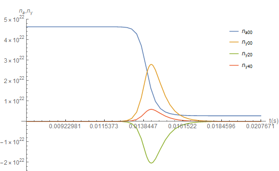
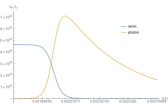
Figure 1: Axion and photon number density components of $n_{a00}$ and ($n_{\gamma 00}$, $n_{\gamma 20}$, $n_{\gamma 40}$) in the non-spherical (left) and spherically symmetrical (right) setups with the same initial axion number density $n_{a00}\sim 4.8\times 10^{22}$, respectively.

Here are a few observations. The whole decay process is slightly delayed in the non-spherical setup in comparison with that of the spherically symmetrical one. The reason behind this is that the evolution of the axion cluster is dominated by the stimulated emission rather than the spontaneous one. However, there is a cancelation between various interaction terms on the right-hand side of Eqs. (16), which leads to the decrease of the rate of the stimulated emission and thus make slow the whole process. In the spherically symmetrical setup, axions totally disappear after some time, while in the non-spherical case there are still residue axions left. Note that on the spherically symmetrical plot, when the photon number density reaches its peak, the axion number density is already very low comparing to that of the photon. Thus, there are enough photons to stimulate axions to decay, and the axion number density quickly drops to nearly zero. This is not the case on the non-spherical plot. When the photon number densities $n_{\gamma 00}$ and $n_{\gamma 20}$ reach their peak values, there are still quite some amount of axions remaining in the cluster. The amount of photons after the peak may not be enough to trigger all the axions to fast decay. As a result, in the end some amount of axions remain.

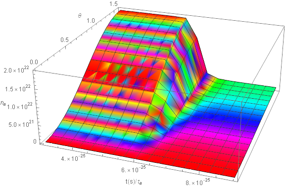
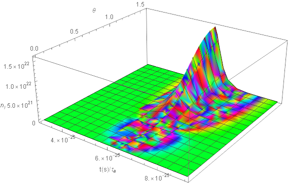
Figure 2: The axion (left) and photon (right) number densities as functions of polar angular $\theta$ and time $t$. The time ticks represent the real time divided by the axion lifetime $\tau_{a}\approx 2.3\times 10^{22}$ s.

In Fig. 2, we also plot the total number densities of axions $n_{a}$ (left panel) and photons $n_{\gamma}$ (right panel) as functions of both polar angle $\theta$ and dimensionless time $t/\tau_{a}$ with $\tau_{a}\approx 2.3\times 10^{22}$ s according to Eq. (2). It is shown in the right panel of Fig. 2 that the stimulated emission is strongest on the equatorial plane with $\theta=\pi/2$ and it diminishes as $\theta$ decreases. Close to the polar area where $\theta\sim 0$, this effect does not manifest itself, which can be understood by the angular distribution of the axion in the mode of $(l,m)=(1,1)$. Our plots in Figs. 1 and 2 illustrate the general features of how the stimulated emission occurs for a non-spherical axion cluster without axion sources.

Finally, we would like to point out the importance of the inclusion of the photon component $n_{\gamma 40}$ in our numerical solutions, even though there is no direct spontaneous emissions from axions to feed into it. In order to show this point, we solve the evolution equations in Eq. (16) again but this time we do not consider the photon density component $n_{\gamma 40}$ and its associated equation. The final results are plotted in Fig. 3.

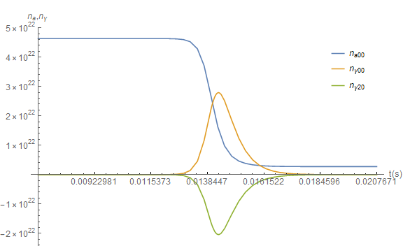
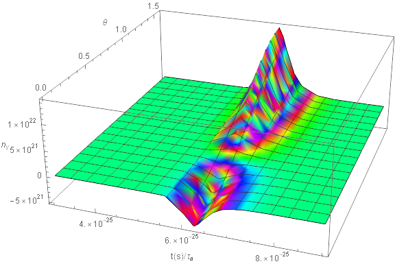
Figure 3: The left panel shows the axion number density component $n_{a00}$ and photon number density components $n_{\gamma 00}$ and $n_{\gamma 20}$ in the non-spherical setup that resembles the superradiance state of $(l,m)=(1,1)$, without introducing the component $n_{\gamma 40}$. The right panel demonstrates the evolution of $n_{\gamma}$ at $\theta$ ($0<\theta<\pi/2$) in this setup with the time ticks representing the real time $t$ divided by the axion lifetime $\tau_{a}$.

It is seen from the left panel that, without introducing $n_{\gamma 40}$, the evolution of densities of axions $n_{a00}$ and photons $n_{\gamma 00(20)}$ is very similar to the results given in the left panel of Fig. 1 in the presence of $n_{\gamma 40}$. However, the difference is clearly seen on the right panel of Fig. 3, where there is a negative photon number density trough when $\theta$ approaches 0. This negative number density near the polar regions infers that the whole system being truncated at $n_{\gamma 20}$ is not complete. Other components such as $n_{\gamma 40}Y_{40}$ should get involved in the process even if there is no spontaneous emission into these components. In contrast, if we add $n_{\gamma 40}$ and its related evolution equations as in Eq. (16), the trough caused by the negative number density around $\theta\simeq 0$ disappears as shown in Fig. 2, which indicates the necessity to include the component $n_{\gamma 40}$ in order to obtain a consistent and complete description of the stimulated emission in the non-spherical situation.

IV Stimulated Emission of a Non-spherical Axion Distribution with Axion Source from Superradiance

In the last section, we have only considered the stimulated emission in the case with a source-free axion cluster. On the other hand, if there is a highly rotating black hole in the center of the cluster, it is generally expected that axions can be continuously produced via the superradiance effect. In other words, we should consider the stimulated emission in presence of the axion source from the black hole superradiance. Note that this situation has already been studied in Ref. [18]. We have reproduced the resultant axion and photon pulses in Fig. 4 but with a different initial conditions. Here, the axion and black hole mass are taken to be $m_{a}=10^{-5}$ eV and $M=8\times 10^{23}$ kg, respectively. It is shown in Fig. 4 that the photon pulses from the axion stimulated emission are uniformly repeated in both pace and amplitude. Due to the similarities of the yielded photon emission with the FRB spectra, Ref. [18] has also pointed out the possible explanation of the mysterious FRBs as the stimulated emission in the black-hole sourced axion clusters. We would like to mention that the above spectra are obtained from the coupled differential evolution equations derived in Ref. [17], where the spherical symmetry has been implicitly used. However, it is well-known that the axions from a Kerr black hole superradiance should be dominantly distributed in the $(l,m)=(1,1)$ mode, which is obviously non-spherical. Thus, it is necessary to revisit the stimulated emission with axions sourced by the black hole superradiance again by applying Eq. (16) for a genuine non-spherical setup, which is the main goal of the present section.

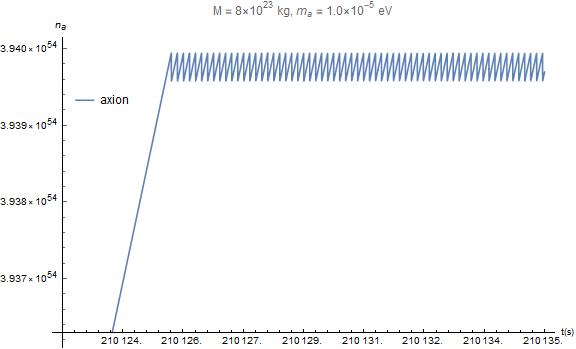
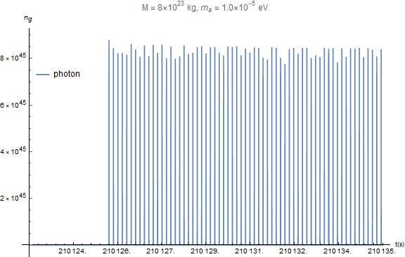
Figure 4: Similar to Fig. 2 in Ref. [18] but with different initial conditions of the axion and black hole masses as $m_{a}=10^{-5}$ eV and $M=8\times 10^{23}$ kg, respectively. The left (right) panel shows evolution of the axion (photon) number density in a spherically symmetric system.

For completeness, we rewrite the basic evolution equations given in Ref. [19] for the superradiance-lasing mechanism in a non-spherical cluster and modified by including an axion source term accounting for the axion exponential growth from the black hole superradiance

$${dn_{a00}\over dt}= \Gamma_{n}n_{a00}-\frac{n_{a00}}{\tau_{a}}-{E_{00}\over 2\beta}+{\beta\over 6}F_{00},\qquad{dn_{\gamma 00}\over dt}=\frac{2n_{a00}}{\tau_{a}}+{E_{00}\over\beta}-({\beta\over 3}+{1\over 2})F_{00}-\Gamma_{e}n_{\gamma 00}$$

$${dn_{a20}\over dt}= \Gamma_{n}n_{a20}-\frac{n_{a20}}{\tau_{a}}-{E_{20}\over 2\beta}+{\beta\over 6}F_{20},\qquad{dn_{\gamma 20}\over dt}=\frac{2n_{a20}}{\tau_{a}}+{E_{20}\over\beta}-\left({\beta\over 3}+{1\over 2}\right)F_{20}-\Gamma_{e}n_{\gamma 20}$$

$${dn_{a40}\over dt}= -\frac{n_{a40}}{\tau_{a}}-{E_{40}\over 2\beta}+{\beta\over 6}F_{40},\qquad{dn_{\gamma 40}\over dt}=\frac{2n_{a40}}{\tau_{a}}+{E_{40}\over\beta}-({\beta\over 3}+{1\over 2})F_{40}-\Gamma_{e}n_{\gamma 40}\,.$$ (17)

where $E_{lm}$ and $F_{lm}$ are coefficients of the modes $Y_{lm}$ in $n_{a}n_{\gamma}$ and $n_{\gamma}^{2}$, respectively, and $\Gamma_{n}$ is the growth rate induced by the imaginary part of the frequency in Eq. (3). We still need to extract $E_{lm}$ and $F_{lm}$ from products $n_{a}n_{\gamma}$ and $n_{\gamma}^{2}$, given by

$$n_{a}n_{\gamma}= E_{00}Y_{00}+E_{20}Y_{20}+E_{40}Y_{40},\qquad n_{\gamma}^{2}=F_{00}Y_{00}+F_{20}Y_{20}+F_{40}Y_{40},$$ (18)

respectively. The total axion and photon number densities $n_{a}$ and $n_{\gamma}$ can be decomposed into the spherical harmonic components as follows

$$n_{a}=n_{a00}Y_{00}+n_{a20}Y_{20}+n_{a40}Y_{40}\,,\qquad n_{\gamma}=n_{\gamma 00}Y_{00}+n_{\gamma 20}Y_{20}+n_{\gamma 40}Y_{40}\,,$$ (19)

respectively. According to the general argument [14], the axion wave function arising from the black hole superradiance should be dominated by the $(l,m)=(1,1)$ mode proportional to $Y_{1}^{\pm 1}$, which results in the initial number density of the axion depending on $Y_{1}^{\pm 1*}Y_{1}^{\pm 1}\propto\sin^{2}\theta\propto Y_{00}-\sqrt{1/5}Y_{20}$. As found in the previous section, we also include $n_{a(\gamma)40}$ for completeness of our computation.

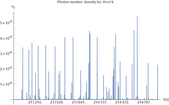
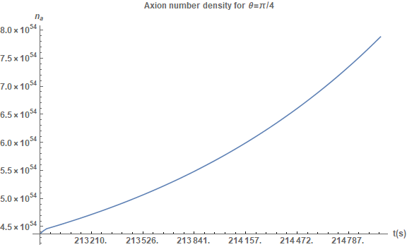
Figure 5: Numerical solutions to Eq. (IV) for $\theta=\pi/2$ (top two plots) $\pi/4$ (bottom two plots).

By solving differential equations in Eq. (IV), we can yield the evolution of number densities of photons and axions in the direction of the polar angle $\theta=\pi/2$ and $\theta=\pi/4$ as displayed in Fig. 5. On the equatorial plane with $\theta=\pi/2$, the axion number density is high at the beginning, so that the stimulated emission rate increases with the accumulation of emitted photons. As the photon density further becomes larger, the depletion of axions from stimulated emissions begins to be faster than the supply of axions from superradiance, so that the axion number density in the cluster has reached its maximal value and starts deceasing. In comparison, at $\theta=\pi/4$, the axion number density keeps increasing because the production of axions from the black hole superradiance is always faster than their loss due to the stimulated emission. The reason is that there are not enough photons created along this direction to deplete axions and to make axion density to decrease.

During this redistribution of the axion number density, photon pulses of different peak amplitudes are released, which can be seen on the left two plots in Fig. 5. The pulses are sharp and randomly distributed in time, and the magnitudes of the sharp pulses are more than 10 times larger than those of the mild ones. This is contrasted with the nearly uniformly repeating feature of the pulses from the spherically symmetric axion cluster shown as in Fig. 4 with the magnitude of pulses differing by less than 10%.

The question of whether the axion cloud in the growing mode $(l,m)=(1,1)$ is able to maintain its “eigenstate” shape is not discussed in previous works in which the evolution process is approximated by fixing the spherical shape of the cluster. Here, our initial condition is set in the mode $(l,m)=(1,1)$ by the relation $n_{a20}(0)=-\sqrt{1/5}n_{a00}(0)$. It turns out that, once the stimulated emission becomes important, the shape of the axion cloud may evolve and cannot stay in the eigenstate $(l,m)=(1,1)$. This feature becomes more transparent in Fig. 6 that the ratio $n_{a20}/n_{a00}$ starts to deviate away from $-\sqrt{1/5}$.

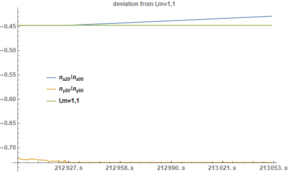
Figure 6: Deviation of the ratios $n_{a20}/n_{a00}$ and $n_{\gamma 20}/n_{\gamma 00}$, comparing to the initial ratio $n_{a20}/n_{a00}$ in the $(l,m)=(1,1)$ state.

The angular distributions of photons are noticeably different from those of axions as shown in Figs. 6 and 7. Especially, the ratio $n_{\gamma 20}/n_{\gamma 00}$ becomes smaller as the system evolves, and deviates more from the $(l,m)=(1,1)$ distribution. The above observation can be understood as follows. Initially, the axion cloud is in the $2p$ mode with $(n,l,m)=(2,1,1)$, in which the axion density concentrates on the equatorial plane, whereas there are much less axions along the polar direction. The evolution induced by the spontaneous and stimulated emissions gradually moderates this difference by decreasing $|n_{a20}/n_{a00}|$. On the other hand, the photon distribution in the cloud becomes to skew to the equatorial plane, which is compared to that of the axion. The skewness of the axion distribution is directly related to its initial $(l,m)=(1,1)$ wave function, while the photon shape is caused by the non-linear nature of the stimulated decay. The initiation of the stimulated emission requires quite a large density of axions. Therefore, in the direction of higher latitude, the axion cloud becomes less dense so that it cannot make the stimulated emission to be significant. This results in fewer photons produced at high latitude, which explains the skewness of the photon angular shape.

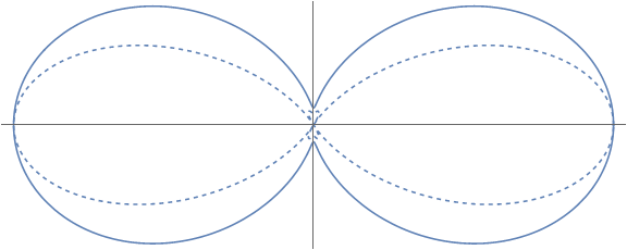
Figure 7: Comparison of the cross-sections of the angular distribution of axions (solid) in the $(l,m)=(1,1)$ mode and photons (dashed) when $n_{\gamma 20}/n_{\gamma 00}=-0.75$.

We have displayed in Fig. 7 the typical cross sections of $Y_{00}+(n_{a20}/n_{a00})Y_{20}$ and $Y_{00}+(n_{\gamma 20}/n_{\gamma 00})Y_{20}$ in polar coordinates when $n_{\gamma 20}/n_{\gamma 00}=-0.75$. If one maps the horizontal and vertical ranges of the solid and dashed curves in Fig. 7 to the radii of two tori, then the cross sections of the axion and photon distributions can be visualized as donut-shped clouds in Fig. 8. It is clear that the photon shape seems to be a slimmer version of the axion cloud, which is consistent with its feature of the further skewness towards the equatorial plane.

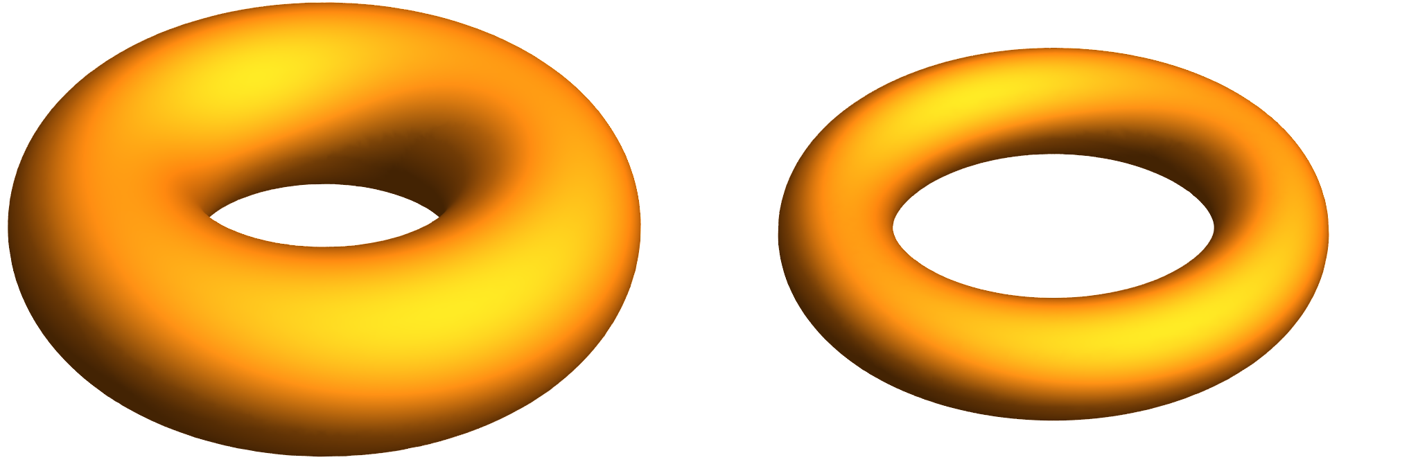
Figure 8: Visualization of axion and photon distributions as torus models.

By observing from the right two panels of Fig. 5 that the axion density on the equatorial plane decreases while $n_{a}$ at $\theta=\pi/4$ increases in the time period of the simulation, we expect that these two curves should coincide at some late time, which means that the axion densities at these two directions will then become the same. In order to prove this expectation, we solve the differential equations in Eq. (IV) again but with a longer time period and at more directions with $\theta=$ $\pi/2$, $2\pi/5$, $\pi/3$, $\pi/4$, $\pi/6$, $\pi/8$, and $0$, respectively.

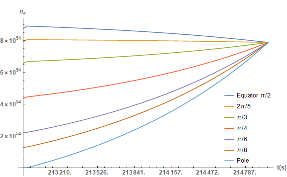
Figure 9: Uniformization of a non-spherical axion cluster initially at the mode $(l,m)=(1,1)$.

The result is shown in Fig. 9. Indeed, all curves that represent the axion densities in different directions intersect exactly at the same magnitude simultaneously, which infers that the distribution of axions becomes spherically symmetrical. We can explain this result by noticing the fact that, beginning at the $l=m=1$ state, the loss of axions from the stimulated emission overcomes the superradiant growth in the equatorial region with initial high axion densities while the opposite takes place in the polar region with low axion densities. In the end, the interplay of the stimulated emission and the black hole superradiance will reach a balance in which the entire axion cloud approaches a uniform distribution, i.e., the axion wave function would transit from $(l,m)=(1,1)$ to $(l,m)=(0,0)$. The lost angular momentum could be transferred from axions into photons, which is manifested in the more and more skew photon distribution towards the equatorial plane.

V Discussion

After the intersection point in Fig. 9, the axion cloud becomes uniform. For the axion and black hole masses considered in the present paper, we find that the axion density restrains growing when its state approaches the shape of $(l,m)=(0,0)$, since at this stage the axion density is still high so that the rate of the stimulated emission dominates over the axion production from the superradiance. Therefore, the axion source from superradiance can be ignored at this moment. This is very similar to the case studied in Ref. [17] which considered an axion source-free cluster with spherical symmetry. The observable signal for this case would be one photon pulse with a very short duration and a very large amplitude as depicted on the right panel of Fig. 1. The released total energy in this end pulse would be several orders of magnitude higher than those in the cloud uniformization process discussed in Sec. IV. Also displayed in Fig. 1, for the spherically symmetric system, accompanied by this final photon pulse is the nearly depletion of the axion number density. In particular, the axion number density is so low that the spontaneous and stimulated emission nearly stops while the black hole superradiance becomes efficient again to build up the axion cluster in the $(l,m)=(0,0)$ mode, which returns to the starting point of our discussion in Sec. IV.

From the above discussion, we find that the evolution of this axion cluster is actually in a cycle which can be summarized as follows: the cycle begins with a low-density axion “fog” which becomes growing due to the superradiance from a center rotating black hole. The fastest growing mode corresponds to $(l,m)=(1,1)$ which indicates that there is an angular variation in the number density of axions. The stimulated emission efficiency strongly depends on the axion density: around the equatorial plane, the axion density is so high that the stimulated emission depletes the axion faster than the axion production rate of the superradiance, which decreases the axion density there. On the other hand, when approaching the polar region, less and less axions distributed there in the initial $(l,m)=(1,1)$ state, so that the black hole superradiance dominates over the stimulated emission and the axion density becomes increased. The combined effect of the stimulated emission and superradiance is that the axion cloud would transform into a state with $(l,m)=(0,0)$, i.e., axions becomes to be uniformly distributed. At this stage, the stimulated emission dominates over the superradiance in all directions, and the axion density refrains to increase. At the end of this uniform-density stage, there is a cycle-end pulse, i.e., a short-duration photon pulse with very high luminosity caused by the stimulated emission. After that, the system returns to a state of a low-density axion fog, and the black hole superradiance restart a new cycle.

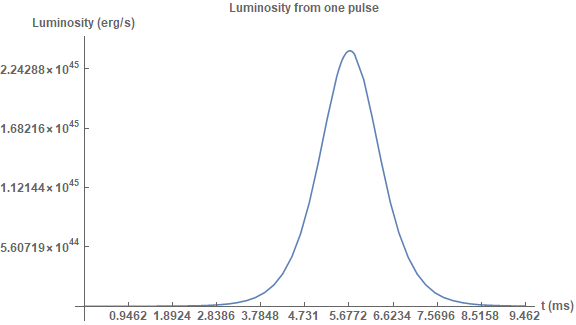
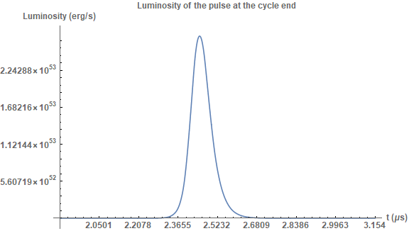
Figure 10: The left panel shows the total energy of photons from one pulse before the cycle end, which is derived from one of the spikes on the left panel of Fig. 5. The right panel shows the energy and duration of a typical cycle-end pulse.

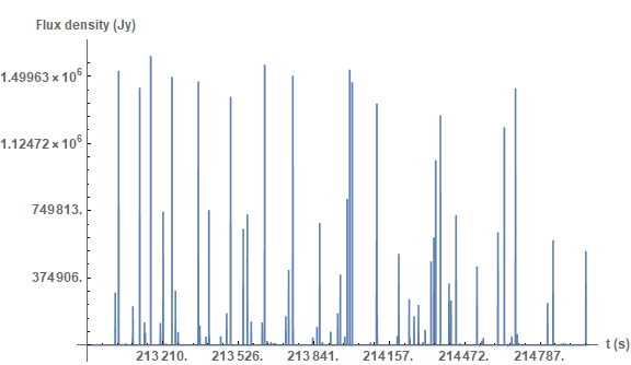
Figure 11: Photon flux density received on the Earth without any attenuation.

It is seen from the above discussion that there are two kinds of observable pulse signals in a dynamical cycle: one is emitted during the uniformization process of the axion cloud and the other corresponds to the cycle-end pulse. We depict the typical spectra for these two signals in Fig. 10. The left panel shows that the duration and frequency of the pulse produced when the axion cloud uniformization are around 1$\sim$2 ms and 1200 MHz, respectively. The total luminosity can be as high as $10^{45}$ erg/s, while total energy released for the pulse duration can reach beyond $10^{42}$ erg. Note that this energy is very close to a recent study that uses a burst energy of $2\times 10^{42}$ erg to revise the maximum energy of FRB 20220610A [22]. The right panel of Fig.10 illustrates that the cycle-end pulse is characterized by the duration of ${\cal O}(\mu s)$ and the luminosity of ${\cal O}(10^{53}\,{\rm erg/s})$, which can be clearly distinguished from the multiple pulses released in the earlier uniformization procedure. We can also show in Fig. 11 the signal strengths of the pulses in terms of the flux density, which is more commonly used in astronomy. The unit of this quantity is “Jansky”. For a source placed in the luminosity distance of $\sim 6700$ Mpc corresponding to the cosmological redshift $z=1$, the fluence and duration of the pulses before the cycle end is of order of $10^{5}$ to $10^{6}$ Jy-ms and a few milliseconds, and those of a cycle-end pulse can be as high as ${\cal O}(10^{10}\,\mbox{Jy-ms})$ and as short as a fraction of one microsecond, respectively.

Due to the similarity in the duration and luminosity shown in Figs. 10 and 11, the pulses from the stimulated emission from axion clouds can be used to explain the observed FRBs. We can compare our predicted signals with the detailed information of FRBs given in the catalogs [24, 23]. For instance, at 1.4 GHz, a 30 Jy pulse of duration less than 5 ms was found and associated with an extragalactic singular event [25]. Additional millisecond-duration FRBs centered at 1.38 GHz with redshifts of 0.5 to 1 were detected and the energy released ranges from $10^{31}$ J to $10^{33}$ J [26], which are close to our estimated energy in Fig. 10. Eight repeating bursts from FRB 121102 were detected in a single day [27] in 2015, the timing of which is consistent with the temporal locations of the pulses plotted in Fig. 11, with the possible sources of these repeating bursts to be low-luminosity active galactic nucleus [28] or a young neutron star energizing a supernova remnant [29]. Because of the measured redshift of $z=0.19$, the origin of FRB 121102 was firmly placed at a cosmological distance [30]. Our estimates on the photon fluence seem to be much larger than these from the signals in the FRB observations. However, it is straightforward to obtain different signal strengths by adjusting many parameters such as the axion and black hole masses as well as axion-photon coupling constant. We can also change our prediction by considering many astrophysical factors, like the curve spacetime geometry, absorption, attenuation and dispersion from the intergalactic media on the path. We compare the characteristics of pulses yielded in our axion cluster setup and those from observations of a few FRBs in Table. 1. On the other hand, FRB measurements also constrained the allowed parameter space for axions or axion like particles, as shown in Ref. [31]. Besides, the author in Ref. [32] proposed the opposite situation that FRBs may convert to axion bursts.

		duration	fluence/flux density	frequency
theory	pulses before cycle end	a few ms	$10^{5}$ to $10^{6}$ Jy-ms	1.2 GHz (z=0)
	cycle end pulse	a fraction of $\mu$s	$10^{10}$ Jy-ms	1.2 GHz (z=0)
observations	FRB 010824[25]	5 ms	30 Jy	1.4 GHz
	FRB 110220[26]	0.8 ms	8 Jy-ms	1.3 GHz
	FRB 121102[27](repeater)	3 to 8 ms	0.06 to 1 Jy-ms	1.4 GHz

Table 1: Comparison of characteristics between the pulses predicted by the stimulated emission in axion clusters and those from a few FRB measurements. In the 4th column, the flux density of FRB 010824 and the fluence of other FRBs are given.

We note that other types of mechanisms involving axions may also be able to explain FRBs. One of the proposed origins of FRBs is the collision of a neutron star and an axion star [33], and the Doppler shift links to the FRB spectral characteristics [34]. A similar idea of the axion star moving in the magnetosphere of a neutron star has been investigated in Ref. [35]. The coherent burst of radiation from gravitationally self-bound axion clusters is also linked to FRBs in Ref. [36]. The possibility that axion quark nuggets falling into a magnetar’s atmosphere and triggering FRBs is discussed in Ref. [37].

VI Conclusion

We have presented an updated evolution model of the stimulated emission from a non-spherical axion cluster, specifically for the initial distribution corresponding to the axion growth mode $(l,m)=(1,1)$ from the black hole superradiance. In the case where there is only an axion cluster without an axion source, the stimulated photon emission is the strongest on the equatorial plane and becomes weaker towards the polar regions. As a result, the entire process releases only one large pulse of photons. On the other hand, when the black hole superradiance acts as the axion production source, the simulated emission and the superradiant growth would interplay with each other, and finally reach a balance point where the axion cloud becomes uniformly distributed. Numerous pulses of different magnitudes are released during this uniformization process. The resultant uniform high-density axion cloud quickly decays and emits a short-duration but high-intensity pulse. After that, the axion cluster returns to a low-density state and it would be rebuilt by the axions in the $(l,m)=(1,1)$ mode generated by the superradiance. This would restart the superradiance-stimulated-emission cycle in the axion-black hole system. The energy and temporal characteristics of the obtained photon pulses could be applicable to the observed FRB phenomena.

- [1] R. D. Peccei and H. R. Quinn, Phys. Rev. Lett. 38, 1440-1443 (1977) doi:10.1103/PhysRevLett.38.1440
- [2] S. Weinberg, Phys. Rev. Lett. 40, 223-226 (1978) doi:10.1103/PhysRevLett.40.223
- [3] S. Barshay, H. Faissner, R. Rodenberg and H. De Witt, Phys. Rev. Lett. 46, 1361-1364 (1981) doi:10.1103/PhysRevLett.46.1361
- [4] A. Barroso and N. C. Mukhopadhyay, Phys. Lett. B 106, 91-94 (1981) doi:10.1016/0370-2693(81)91087-X
- [5] J. E. Kim, Phys. Rev. Lett. 43, 103 (1979) doi:10.1103/PhysRevLett.43.103
- [6] M. A. Shifman, A. I. Vainshtein and V. I. Zakharov, Nucl. Phys. B 166, 493-506 (1980) doi:10.1016/0550-3213(80)90209-6
- [7] M. Dine, W. Fischler and M. Srednicki, Phys. Lett. B 104, 199-202 (1981) doi:10.1016/0370-2693(81)90590-6
- [8] A. R. Zhitnitsky, Sov. J. Nucl. Phys. 31, 260 (1980)
- [9] G. Grilli di Cortona, E. Hardy, J. Pardo Vega and G. Villadoro, JHEP 01, 034 (2016) doi:10.1007/JHEP01(2016)034
- [10] S. L. Cheng, C. Q. Geng and W. T. Ni, Phys. Rev. D 52, 3132-3135 (1995) doi:10.1103/PhysRevD.52.3132
- [11] S. L. Detweiler, Phys. Rev. D 22, 2323-2326 (1980) doi:10.1103/PhysRevD.22.2323
- [12] T. J. M. Zouros and D. M. Eardley, Annals Phys. 118, 139-155 (1979) doi:10.1016/0003-4916(79)90237-9
- [13] S. R. Dolan, Phys. Rev. D 76, 084001 (2007) doi:10.1103/PhysRevD.76.084001
- [14] R. Brito, V. Cardoso and P. Pani, Physics,” Lect. Notes Phys. 906, pp.1-237 (2015) 2020, ISBN 978-3-319-18999-4, 978-3-319-19000-6, 978-3-030-46621-3, 978-3-030-46622-0 doi:10.1007/978-3-319-19000-6
- [15] I. I. Tkachev, Sov. Astron. Lett. 12, 305-308 (1986)
- [16] T. W. Kephart and T. J. Weiler, Phys. Rev. Lett. 58, 171 (1987) doi:10.1103/PhysRevLett.58.171
- [17] T. W. Kephart and T. J. Weiler, Phys. Rev. D 52, 3226-3238 (1995) doi:10.1103/PhysRevD.52.3226
- [18] J. G. Rosa and T. W. Kephart, Phys. Rev. Lett. 120, no.23, 231102 (2018) doi:10.1103/PhysRevLett.120.231102
- [19] L. Chen and T. W. Kephart, Phys. Rev. D 102, no.9, 096010 (2020) doi:10.1103/PhysRevD.102.096010
- [20] M. P. Hertzberg and E. D. Schiappacasse, JCAP 11, 004 (2018) doi:10.1088/1475-7516/2018/11/004
- [21] D. B. Kaplan, Nucl. Phys. B 260, 215-226 (1985) doi:10.1016/0550-3213(85)90319-0
- [22] S. D. Ryder, K. W. Bannister, S. Bhandari, A. T. Deller, R. D. Ekers, M. Glowacki, A. C. Gordon, K. Gourdji, C. W. James and C. D. Kilpatrick, et al. Science 392, 294-299 (2023) doi:10.1126/science.adf2678
- [23] E. Petroff, E. D. Barr, A. Jameson, E. F. Keane, M. Bailes, M. Kramer, V. Morello, D. Tabbara and W. van Straten, Publ. Astron. Soc. Austral. 33, e045 (2016) doi:10.1017/pasa.2016.35
- [24] M. Amiri et al. [CHIME/FRB], Astrophys. J. Supp. 257, no.2, 59 (2021) doi:10.3847/1538-4365/ac33ab
- [25] D. R. Lorimer, M. Bailes, M. A. McLaughlin, D. J. Narkevic and F. Crawford, Science 318, 777 (2007) doi:10.1126/science.1147532
- [26] D. Thornton, B. Stappers, M. Bailes, B. R. Barsdell, S. D. Bates, N. D. R. Bhat, M. Burgay, S. Burke-Spolaor, D. J. Champion and P. Coster, et al. Science 341, no.6141, 53-56 (2013) doi:10.1126/science.1236789
- [27] L. G. Spitler, P. Scholz, J. W. T. Hessels, S. Bogdanov, A. Brazier, F. Camilo, S. Chatterjee, J. M. Cordes, F. Crawford and J. Deneva, et al. Nature 531, 202 (2016) doi:10.1038/nature17168
- [28] S. Chatterjee, C. J. Law, R. S. Wharton, S. Burke-Spolaor, J. W. T. Hessels, G. C. Bower, J. M. Cordes, S. P. Tendulkar, C. G. Bassa and P. Demorest, et al. Nature 541, 58 (2017) doi:10.1038/nature20797
- [29] B. Marcote, Z. Paragi, J. W. T. Hessels, A. Keimpema, H. J. van Langevelde, Y. Huang, C. G. Bassa, S. Bogdanov, G. C. Bower and S. Burke-Spolaor, et al. Astrophys. J. Lett. 834, no.2, L8 (2017) doi:10.3847/2041-8213/834/2/L8
- [30] S. P. Tendulkar, C. Bassa, J. M. Cordes, G. C. Bower, C. J. Law, S. Chatterjee, E. A. K. Adams, S. Bogdanov, S. Burke-Spolaor and B. J. Butler, et al. Astrophys. J. Lett. 834, no.2, L7 (2017) doi:10.3847/2041-8213/834/2/L7
- [31] A. Caputo, L. Sberna, M. Frias, D. Blas, P. Pani, L. Shao and W. Yan, Phys. Rev. D 100, no.6, 063515 (2019) doi:10.1103/PhysRevD.100.063515
- [32] A. Prabhu, Astrophys. J. Lett. 946, no.2, L52 (2023) doi:10.3847/2041-8213/acc7a7
- [33] A. Iwazaki, Phys. Rev. D 91, no.2, 023008 (2015) doi:10.1103/PhysRevD.91.023008
- [34] A. Iwazaki, PTEP 2020, no.1, 013E02 (2020) doi:10.1093/ptep/ptz142
- [35] J. H. Buckley, P. S. B. Dev, F. Ferrer and F. P. Huang, Phys. Rev. D 103, no.4, 043015 (2021) doi:10.1103/PhysRevD.103.043015
- [36] I. I. Tkachev, JETP Lett. 101, no.1, 1-6 (2015) doi:10.1134/S0021364015010154
- [37] L. van Waerbeke and A. Zhitnitsky, Phys. Rev. D 99, no.4, 043535 (2019) doi:10.1103/PhysRevD.99.043535