Diameter of Uniform Spanning Trees on Random Weighted Graphs

Abstract.

For any edge weight distribution, we consider the uniform spanning tree (UST) on finite graphs with i.i.d. random edge weights. We show that, for bounded degree expander graphs and finite boxes of $\mathbb{Z}^{d}$, the diameter of the UST is of order $n^{1/2+o(1)}$ with high probability, where $n$ is the number of vertices.

1. Introduction

1.1. Background and Main Result

Let $(G,w)$ be a connected weighted finite graph, where $G=(V,E)$ has vertex set $V$ and edge set $E$, and $w:=(w_{e})_{e\in E}$ are the weights (or conductances) assigned to the edges, with $w_{e}>0$ for all $e\in E$. A spanning tree $T$ of $G$ is a cycle–free connected subgraph of $G$ with the same vertex set $V$. We identify $T$ with its own edge set and write $\mathbb{T}=\mathbb{T}(G)$ for the set of all spanning trees on $G$. The uniform spanning tree (UST) on $(G,w)$ is then defined to be the random spanning tree ${\mathcal{T}}$ on $G$ with probability distribution

$$\boldsymbol{\mathrm{P}}^{w}({\mathcal{T}}=T)=\frac{1}{Z}\prod_{e\in T}w_{e}\qquad\mbox{with }\ Z=Z(w):=\sum_{T\in\mathbb{T}}\prod_{e\in T}w_{e}\,.$$ (1.1)

The UST is a fundamental object in combinatorics and probability, which has interesting connections to electric networks, loop erased random walks, percolation, dimers and many other topics, see e.g. [24, 11, 20, 18] for more background on the UST. We point out that most studies of the UST are on unweighted graphs where $w\equiv 1$.

One fundamental question concerns the scaling limits of the UST on sequences of large finite graphs. To identify the limit, the first step is to identify the correct order of the diameter $diam({\mathcal{T}})$, that is, the maximal graph distance in the UST between any pair of vertices. For unweighted “high-dimensional” graphs, such as the complete graph, finite tori in dimension $d\geq 5$, expanders and dense graphs, it has been shown in [30, 6, 14, 25, 21, 8] that the diameter of the UST is typically of order $\sqrt{n}$, where $n$ is the number of vertices in the graph. In fact, it is believed that, seen as a random metric space equipped with the graph distance, the UST rescaled by $1/\sqrt{n}$ would converge in distribution to Aldous’ continuum random tree (CRT) [2, 3, 4]. This was verified in the Gromov-Hausdorff topology for the complete graph in [2, 3, 4], in finite-dimensional distribution for finite tori in dimension $d\geq 5$ and $d=4$ in [25] and [28] respectively, and in the stronger Gromov-Hausdorff-Prohorov topology for finite tori in dimension $d\geq 5$ in [9] and for dense graphs in [10].

Our goal in the present work is to initiate the study of the UST on random weighted graphs with i.i.d. edge weights, which defines a disordered system similar to random walks in random environment, a topic that has been studied extensively, see e.g. [31, 32]. The basic question is how the random environment affects the behaviour of the UST. More specifically, we study the diameter of the UST in a typical environment. We point out that the techniques developed for unweighted graphs, such as in [21], no longer apply when the edge weights are not uniformly bounded away from $0$ and $\infty$. We will treat two separate cases for the underlying graph: expander graphs with bounded degrees (see Section 2.2 for the proper definition) and boxes in the $\mathbb{Z}^{d}$ lattice, with $d\geq 5$. We show that in both cases, regardless of the edge weight distribution, the diameter of the UST in a typical random environment is of order $\sqrt{n}$ modulo a factor of $(\log n)^{c}$. Our main result is the next theorem.

Theorem 1.1.

Let $G=(V,E)$ be a graph with $|V|=n$, which is either of the following:

• a $b$-expander graph for some $b>0$ with maximum degree $\Delta<\infty$;

• the box $[-L,L]^{d}\cap\mathbb{Z}^{d}$ of volume $n$, for some $d\geq 5$.

Let $(w_{e})_{e\in E}$ be i.i.d. random edge weights with common distribution $\mu$ satisfying $\mu(0,\infty)=1$. Denote probability and expectation w.r.t. $w$ by $\mathbb{P}$ and $\mathbb{E}$. Given $w$, let $\mathcal{T}$ be the UST on the weighted graph $(G,w)$ defined as in (1.1), with its law denoted by $\boldsymbol{\mathrm{P}}^{w}$. Then there exist constants $c,\gamma>0$ not depending on $n$ such that, for all large $n$ and for $\varepsilon>n^{-\gamma}$,

$$\widehat{\mathbb{P}}\left(\frac{\sqrt{n}}{(\varepsilon^{-1}\log n)^{c}}\leq\text{diam}({\mathcal{T}})\leq(\varepsilon^{-1}\log n)^{c}\sqrt{n}\right)\geq 1-\varepsilon\,,$$ (1.2)

where $\widehat{\mathbb{P}}(\cdot)$ denotes the averaged law $\mathbb{E}\boldsymbol{\mathrm{P}}^{w}(\cdot)$.

Remark 1.2.

As we will see in the proof (cf. Remark 4.1 and Remark 5.3), it is in fact possible to choose the exponents of $\log n$ in (1.2) to be a universal constant independent of $b$, $\Delta$ and $\mu$ for the expanders (case $(i)$) or as a constant which only depends on $d$ for the boxes in $\mathbb{Z}^{d}$ (case $(ii)$). The dependency on the other parameters will be present only at the level of a multiplicative constant. Furthermore, in both cases $\gamma$ can be taken as a universal constant.

One may apply Theorem 1.1 as follows.

Remark 1.3.

Consider fixed $\mu$ with $\mu(0,\infty)=1$, $b>0$ and $\Delta<\infty$ and let $(G_{n})_{n\in\mathbb{N}}$, with $|V_{n}|=n$, be a sequence of graphs such that each $G_{n}$ is a $b$-expander with maximum degree at most $\Delta$ and i.i.d. edge weights $w_{n}$ distributed according to $\mu$. Then, since the constants in Theorem 1.1 are independent of $n$, the diameter of ${\mathcal{T}}_{(G_{n},w_{n})}$ is of order $\sqrt{n}$ up to polylogarithmic factors with high probability as $n\to\infty$.

Remark 1.4.

The conclusion in Remark 1.3 cannot hold in general if we drop the condition that graphs in the sequence $(G_{n})_{n\in\mathbb{N}}$ have uniformly bounded maximal degrees, because the upper and lower bounds on $\text{diam}({\mathcal{T}})$ in (1.2) depend on the maximal degree of the graph. For example, in Section 6.1 we show that the diameter of the UST on the complete graph is typically of order $n^{1/3+o(1)}$ if the law of the edge weights is very heavy-tailed.

For further studies, it will be interesting to investigate whether the factors of $(\log n)^{c}$ can be removed from the bounds on the diameter for any choice of $\mu$. If the answer is positive, one could then possibly show convergence along a sequence $G_{n}=(V_{n},E_{n})$ (with $|V_{n}|=n$) to Aldous’ continuum random tree under either the averaged law $\widehat{\mathbb{P}}$, or the quenched law $\boldsymbol{\mathrm{P}}^{w}$ for typical realisations of the random edge weights $w$.

1.2. Proof Strategy

For unweighted graphs $G=(V,E)$, general conditions have been formulated in [21] that imply the diameter of the UST on $G$ to be typically of order $\sqrt{|V|}$. However, these conditions can not be applied in our setting with i.i.d. random edge weights when the support of the edge weight distribution $\mu$ is not bounded away from $0$ and $\infty$.

Our novel idea is to first single out edges whose weights (or conductances) fall inside an interval $[1/A,A]$ for some $A>0$, which form a bond percolation process on $G$ with parameter $p\in(0,1)$ that can be chosen arbitrarily close to $1$ by choosing $A$ large. We then condition on the edge configuration of the UST ${\mathcal{T}}$ on the remaining closed edges, i.e., the edges with weight outside of $[1/A,A]$. This conditioning essentially allows us to consider the UST on a modified graph with edge weights uniformly bounded away from 0 and $\infty$. More precisely, by the spatial Markov property (see Lemma 2.1 below), the conditional law of ${\mathcal{T}}$ on the (open) edges with weights inside $[1/A,A]$ is the same as the law of a UST ${\mathcal{T}}^{\prime}$ on a new graph $G^{\prime}$ (possibly with multiple edges) obtained from $G$, where each closed edge is contracted if it lies in ${\mathcal{T}}$ and deleted if it does not lie in ${\mathcal{T}}$. We will then show that for typical realisations of the random edge weights and uniformly w.r.t. the realisation of ${\mathcal{T}}$ on the closed edges, the graph $G^{\prime}$ satisfies the conditions of Theorem 2.3 below, which is a strengthened version of [21, Theorem 1.1] and implies bounds on the diameter of ${\mathcal{T}}^{\prime}$. Undoing the contractions will then give us the desired bounds on the diameter of ${\mathcal{T}}$.

To verify the conditions in Theorem 2.3 for $G^{\prime}$ in the case of expander graphs, we will analyse the bottleneck ratio (see (2.4)) of $G^{\prime}$ and show that it matches the bottleneck ratio of the unweighted version of $G$ up to polylogarithmic factors. This in turn will give us strong enough bounds on the mixing time of the lazy random walk on $G^{\prime}$ needed to apply Theorem 2.3. For finite boxes in $\mathbb{Z}^{d}$, we will need to go a step further and analyse the whole bottleneck profile (see (5.1)) of $G^{\prime}$ and again show that this is up to polylogarithmic factors the same as that of $G$. Analysing the bottleneck profile instead of the bottleneck ratio allows us to obtain sharper bounds on the random walk transition kernel, which are needed for the case of finite boxes in $\mathbb{Z}^{d}$.

There is hope that this approach can be generalised to arbitrary bounded degree graphs with good enough expansion properties. We refer to (6.2) in Section 6 for the technical condition that is required to extend this result to other graphs.

1.3. Outline

The rest of the paper is organised as follows. In Section 2, we first recall some background material on the UST and expander graphs. We then formulate Theorem 2.3, which gives a variant of the conditions in [21] to bound the diameter of a UST on weighted graphs. In Section 3 we show that the graph $G^{\prime}$ discussed above has good expansion properties, and then in Section 4 we verify the conditions of Theorem 2.3 for $G^{\prime}$ and deduce Theorem 1.1. Section 5 treats the case of finite boxes in $\mathbb{Z}^{d}$ with $d\geq 5$. In Section 6, we give a counter-example to Remark 1.3 where the graph degrees are not uniformly bounded, and we discuss possible extensions to other graphs. Lastly, we sketch in Appendix A the proof of Theorem 2.3.

2. Preliminaries

We recall the spatial Markov property of the UST on a weighted graph $(G,w)$ in Section 2.1 and the definition of edge expansion for $(G,w)$ and its connection to the mixing time of a lazy random walk on $(G,w)$ in Section 2.2. Finally we give conditions that ensure that the UST on $(G,w)$ is of order $|V|^{\frac{1}{2}+o(1)}$ with high probability in Section 2.3.

2.1. Spatial Markov proprety of UST

Given a graph $G=(V,E)$, the contraction of an edge $e\in E$ is the graph $G/e$ obtained by removing $e$ and identifying the endpoints of $e$ as a single vertex. The deletion of $e$ is the graph, denoted by $G-\{e\}$, with vertex set $V$ and edge set $E\backslash\{e\}$. For $A\subseteq E$, the graph $G/A$, resp. $G-A$, is defined as the repeated contraction, resp. deletion, of all edges in $A$, which can be shown to be independent of the order of contraction, resp. deletion.

Given a finite connected weighted graph $(G,w)$, we will let ${\mathcal{T}}_{(G,w)}$ denote the UST on $(G,w)$. The UST is known to satisfy the following spatial Markov property, see e.g. [17, Sec. 2.2.1].

Lemma 2.1.

Let $(G,w)$ be a finite connected weighted graph. Let $A,B\subset E$ be two disjoint sets of edges such that $\boldsymbol{\mathrm{P}}(A\subset{\mathcal{T}}_{(G,w)},B\cap{\mathcal{T}}_{(G,w)}=\emptyset)>0$. Then for any set of edges $F\subset E$,

$$\boldsymbol{\mathrm{P}}({\mathcal{T}}_{(G,w)}=F|A\subset{\mathcal{T}}_{(G,w)},B\cap{\mathcal{T}}_{(G,w)}=\emptyset)=\boldsymbol{\mathrm{P}}({\mathcal{T}}_{((G-B)/A,w)}\cup A=F).$$

Namely, conditioned on ${\mathcal{T}}_{(G,w)}$ containing all edges in $A$ and none of the edges in $B$, the law of ${\mathcal{T}}_{(G,w)}$ restricted to $E\backslash(A\cup B)$ is the same as that of ${\mathcal{T}}_{((G-B)/A,w)}$, the UST on the weighted graph where we have deleted all edges in $B$ and then contracted all edges in $A$.

2.2. Edge expansion and mixing time

Let $G=(V,E)$ be a finite graph. The edge expansion of a set of vertices $S\subset V$ is defined as

$$h_{G}(S):=\frac{|E(S,S^{c})|}{|S|},$$

where $E(S,S^{c})$ denotes the edges between $S$ and $S^{c}:=V\backslash S$. The isoperimetric constant or the Cheeger constant of $G$ (see e.g. [22]) is then defined by

$$h_{G}:=\min\limits_{1\leq|S|\leq\frac{|V|}{2}}h_{G}(S).$$ (2.1)

Given $b>0$, $G$ is called a $b$–expander if $h_{G}\geq b$, which is equivalent to

$$|E(S,S^{c})|\geq b\min\{|S|,|S^{c}|\}\qquad\mbox{for all }S\subset V.$$ (2.2)

The notion of edge expansion and isoperimetric constant can be extended to a weighted graph $(G,w)$ as follows. For $S\subset V$, the analogue of $h_{G}(S)$ is defined by

$$\Phi_{(G,w)}(S):=\frac{\sum_{e\in E(S,S^{c})}w_{e}}{\sum_{x\in S,y\in V}w_{\{x,y\}}},$$ (2.3)

where $w_{\{x,y\}}=0$ if $\{x,y\}\notin E$. This is also called the bottleneck ratio or conductance of $S$. The following quantity, which we will call the bottleneck ratio of $(G,w)$, defines an analogue of the isoperimetric constant for weighted graphs:

$$\Phi_{(G,w)}:=\min\limits_{0<\pi(S)\leq 1/2}\Phi_{(G,w)}(S),\quad\mbox{where}\ \ \pi(S)=\frac{\sum_{x\in S,y\in V}w_{\{x,y\}}}{\sum_{x,y\in V}w_{\{x,y\}}}.$$ (2.4)

We remark that when $G$ is $d$-regular with constant weights, then up to a constant multiple of $d^{-1}$ the definitions in (2.1) and (2.4) match. Furthermore, we note that given $b>0$, $\Phi_{(G,w)}\geq b$ is equivalent to

$$\sum_{e\in E(S,S^{c})}w_{e}\geq b\min\Big{\{}\sum_{x\in S,y\in V}w_{\{x,y\}},\sum_{x\in S^{c},y\in V}w_{\{x,y\}}\Big{\}}\quad\mbox{for all }S\subset V.$$ (2.5)

The bottleneck ratio is closely connected to the mixing time of a reversible random walk on $(G,w)$. To avoid periodicity issues, one typically considers the discrete time lazy random walk $X$ with one-step transition probability

$$q(x,y)=\left\{\begin{aligned} \frac{1}{2}\qquad&\qquad\mbox{ if }x=y,\\ \frac{1}{2}\frac{w_{\{x,y\}}}{\sum_{z}w_{\{x,z\}}}&\qquad\mbox{ if }x\neq y,\end{aligned}\right.$$ (2.6)

and $t$-steps transition probabilities $q_{t}(x,y)$. Then $X$ has stationary distribution

$$\pi(x)=\frac{\sum_{v\in V}w_{\{x,v\}}}{\sum_{u,v\in V}w_{\{u,v\}}},$$ (2.7)

so that we can rewrite

$$\Phi_{(G,w)}(S)=\frac{\sum_{x\in S,y\in S^{c}}\pi(x)q(x,y)}{\pi(S)}.$$ (2.8)

The (uniform) mixing time of $X$ on $(G,w)$ is defined as

$$t_{\text{mix}}(G,w):=\min\left\{t\geq 0:\max\limits_{u,v\in V}\left|\frac{q_{t}(u,v)}{\pi(v)}-1\right|\leq\frac{1}{2}\right\}.$$ (2.9)

We have the following relations between $t_{\text{mix}}(G,w)$ and $\Phi_{(G,w)}$.

Theorem 2.2 (Cheeger Bound).

The mixing time $t_{\text{mix}}(G,w)$ of the lazy walk on $(G,w)$ and the bottleneck ratio $\Phi_{(G,w)}$ satisfy

$$\frac{1}{4\Phi_{(G,w)}}\leq t_{\text{mix}}(G,w)\leq\frac{2\log(2/\pi_{\min})}{\Phi_{(G,w)}^{2}},$$

where $\pi_{\min}=\min_{v\in V}\pi(v)$.

This result goes back to [29], we also refer to Chapters 7, 12 and 13 of [19].

2.3. Diameter of the UST

In [21], the authors considered finite unweighted graphs $G=(V,E)$ with $|V|=n$. Under three conditions on $G$, they showed that the UST on $G$ has diameter of order $\sqrt{n}$ with high probability. We state here the analogue of their conditions for a weighted graph $(G,w)$ and remark that the main difference is in (2.10), which coincides with their original condition when $w\equiv 1$, in which case (2.10) says that the ratio of maximum to minimum degree is bounded. We say that $(G,w)$ is balanced, mixing and escaping with parameters respectively $D,\alpha,\vartheta>0$ if the following are satisfied:

1. $(G,w)$ is balanced if

   $$\frac{\max_{u\in V}\pi(u)}{\min_{u\in V}\pi(u)}=\frac{\max_{u\in V}\sum_{v}w_{\{u,v\}}}{\min_{u\in V}\sum_{v}w_{\{u,v\}}}\leq D;$$ (2.10)

2. $(G,w)$ is mixing if

   $$t_{\text{mix}}(G,w)\leq n^{\frac{1}{2}-\alpha}\,;$$ (2.11)

3. $(G,w)$ is escaping if

   $$\sum_{t=0}^{t_{\text{mix}}}(t+1)\sup_{v\in V}q_{t}(v,v)\leq\vartheta\,.$$ (2.12)

In [21], the bound on the diameter of the UST on an unweighted graph $G$ was formulated in terms of the constants $D,\alpha,\vartheta$ which do not depend on $n$. We formulate here an extension that includes weighted graphs and also allows $D$ and $\vartheta$ to depend on $n$.

Theorem 2.3 (Extension of Theorem 1.1 in [21]).

For any $\alpha>0$, there exist $C,k,\gamma>0$ such that if $(G,w)$ satisfies condition (2.11) with $\alpha$ and conditions (2.10) and (2.12) for some $D=D(n)$ and $\vartheta=\vartheta(n)$ with $D,\vartheta\leq n^{\gamma}$, then for any $\varepsilon>n^{-\gamma}$,

$$\boldsymbol{\mathrm{P}}^{w}\big{(}(CD\vartheta\varepsilon^{-1})^{-k}\sqrt{n}\leq diam({\mathcal{T}}_{(G,w)})\leq(CD\vartheta\varepsilon^{-1})^{k}\sqrt{n}\big{)}\geq 1-\varepsilon.$$ (2.13)

We will apply Theorem 2.3 to $(G,w)$ with $D,\vartheta\leq(\log n)^{c}$ for some $c>0$. The proof of Theorem 2.3 will be sketched in Appendix A.

3. Edge Expansion Bounds

For a weighted graph $(G,w)$ with arbitrary edge weights $w$, the constants $D$ and $\vartheta$ in (2.10) and (2.12) could be so large that the lower and upper bounds on the diameter in Theorem 2.3 become too far apart to be meaningful. This happens in particular when the edge weights are i.i.d. random variables with a very heavy-tailed distribution. In this case, there could be an edge whose weight dominates that of all other adjacent edges and the associated random walk would get stuck on that edge for a long time. As outlined in Section 1.2, we circumvent this problem by conditioning on the UST ${\mathcal{T}}$ restricted to edges whose weights lie outside the interval $[1/A,A]$, which are the closed edges in a percolation process. The conditional distribution of ${\mathcal{T}}$ on the open edges is then a UST ${\mathcal{T}}^{\prime}$ on a new graph $(G^{\prime},w^{\prime})$ (with possibly multiple edges) where closed edges that lie in ${\mathcal{T}}$ have been contracted while closed edges not in ${\mathcal{T}}$ have been deleted. The goal of this section is to give a lower bound on the bottleneck ratio for $(G^{\prime},w^{\prime})$ that is uniform over the realization of ${\mathcal{T}}$ on the closed edges (see Prop. 3.5) and uniform over typical realizations of the edge weights $w$ (that is, $w$ that satisfy the conditions in (3.3)). Thanks to the relation between the bottleneck ratio and the mixing time in Theorem 2.2, this will guarantee that the conditions of Theorem 2.3 for $(G^{\prime},w^{\prime})$ are fulfilled.

We notice that $(G^{\prime},w^{\prime})$ consists only of edges with weights in $[1/A,A]$, so that controlling the isoperimetric constant and the maximum degree in $G^{\prime}$ is sufficient to give good lower bounds for the bottleneck ratio of $(G^{\prime},w^{\prime})$. We accomplish this by comparing $G^{\prime}$ with $\mathcal{C}_{1}$, the largest connected component of open edges in $G$ (i.e., edges with weights in $[1/A,A]$). It is known that for $A$ large enough, the isoperimetric constant of $\mathcal{C}_{1}$ is at least $1/\log|V|$ (see Lemma 3.4). The graph $G^{\prime}$ is obtained from $\mathcal{C}_{1}$ by contracting some closed edges and attaching the vertices outside $\mathcal{C}_{1}$. A crucial observation (see Lemma 3.3) is that $\mathcal{C}_{1}$ disconnects the remaining vertices of $G$ into components of size at most $\log|V|$, which implies that when we attach these components to $\mathcal{C}_{1}$ to obtain $G^{\prime}$, the isoperimetric constant only changes by a factor of $(\log|V|)^{c}$.

In Section 3.1, we state three elementary bounds on percolation cluster sizes. In Section 3.2, we recall a bound on the isoperimetric constant of the largest percolation cluster $\mathcal{C}_{1}$. In Section 3.3, we bound the bottleneck ratio for the weighted graph $G^{\prime}$ described above.

3.1. Bounds on Percolation Clusters Size

Given a finite graph $G=(V,E)$ and a percolation parameter $p\in(0,1)$, we can perform bond percolation on $G$ by independently keeping each edge with probability $p$ and deleting otherwise. Kept edges are also called open, while deleted ones are called closed. In this way, the graph is broken into multiple connected components (or clusters), which are regarded as subgraphs of $G$. For $\ell\in\mathbb{N}$, let $\mathcal{C}_{\ell}=C_{\ell}(p)$ denote the $\ell$-th largest open cluster (ties are broken arbitrarily) and let $|\mathcal{C}_{\ell}|$ denote the number of vertices in $\mathcal{C}_{\ell}$.

We collect here three bounds on the sizes of percolation clusters. The first bound states that for a $b$–expander graph $G=(V,E)$ (cfr. Section 2.2), if $p$ is close enough to $1$, then the size of the largest cluster $\mathcal{C}_{1}$ is at least $\zeta n$, where $\zeta\in(0,1)$ can be made arbitrarily close to $1$ by choosing $p$ close to $1$. In this case, $\mathcal{C}_{1}$ is also called the giant component.

Lemma 3.1.

Let $b>0$. Then for all $\zeta\in(0,1)$, there exists $p_{\zeta}\in(0,1)$ depending only on $b$ such that for all $p\in[p_{\zeta},1]$ and for all $b$-expander graphs $G=(V,E)$ with $|V|=n$,

$$\mathbb{P}(|\mathcal{C}_{1}|\geq\zeta n)\geq 1-{\rm e}^{-n}.$$

Proof.

Given the percolation configuration on $G$ with parameter $p$, and for $A\subset V$, let $E_{p}(A,A^{c})$ denote the set of open edges connecting $A$ and $A^{c}$. For $\zeta\in(0,1)$, let us consider the event

$${\mathcal{H}}(\zeta):=\{\exists\,A\subset V\text{ s.t.\ }|A|\geq\frac{\zeta n}{2},\,\,|A^{c}|\geq\frac{(1-\zeta)n}{2}\,\text{ and }\,E_{p}(A,A^{c})=\emptyset\}\,.$$

Note that if $|\mathcal{C}_{1}|<\zeta n$, then the event ${\mathcal{H}}(\zeta)$ must hold. Indeed, since the clusters $(\mathcal{C}_{\ell})_{\ell\geq 1}$ are decreasing in size, there is some $k\in\mathbb{N}$ such that $|\bigcup_{\ell=1}^{k}\mathcal{C}_{\ell}|\in[\zeta n/2,\zeta n]$. Choosing $A$ to be the vertex set of $\bigcup_{\ell=1}^{k}\mathcal{C}_{\ell}$ then establishes the event ${\mathcal{H}}(\zeta)$.

Since $G$ is a $b$-expander, if ${\mathcal{H}}(\zeta)$ holds, then there exists $A\subset V$ such that

$$|E(A,A^{c})|\geq b\min\{\zeta,1-\zeta\}\frac{n}{2}.$$

The probability that all edges between such $A$ and $A^{c}$ are closed in the percolation configuration is at most $(1-p)^{b\min\{\zeta,1-\zeta\}\frac{n}{2}}$. Thus a union bound over all $A\subset V$ gives

$$\mathbb{P}(\mathcal{H}(\zeta))\leq 2^{n}(1-p)^{b\min\{\zeta,1-\zeta\}\frac{n}{2}}\leq{\rm e}^{-n}$$

provided $p\geq p_{\zeta}:=1-{\rm e}^{-\frac{2(1+\log 2)}{b\min\{\zeta,1-\zeta\}}}$. ∎

The second bound of this section states that in a bounded degree graph with $n$ vertices, for a sufficiently small percolation parameter $p^{\prime}$, the largest open cluster has size at most $\log n$. Equivalently, for $p$ close to $1$, the largest closed clusters are of size at most $\log n$.

Lemma 3.2.

For any $\Delta\in\mathbb{N}$ and $\eta>0$, there exist $C>0$ and $p^{\prime}_{\eta}\in(0,1)$ such that for any $G=(V,E)$ with $|V|=n$ and maximum degree $\Delta$, and for all $p^{\prime}\in[0,p^{\prime}_{\eta}]$,

$$\mathbb{P}(|\mathcal{C}_{1}(p^{\prime})|\geq\log n)\leq\frac{C}{n^{\eta}}\,.$$

Proof.

For $r\in\mathbb{N}$, let $\mathcal{G}_{r}$ denote the set of all possible connected subgraphs of $G$ with $r$ vertices, each of which contains at least $r-1$ edges. For a graph with $n$ vertices and maximal degree $\Delta$, it is known that (see e.g. [7, Proof of Lemma 2.2]) $|\mathcal{G}_{r}|\leq\frac{n}{r}(\Delta{\rm e})^{r}$. A union bound over all connected subgraphs with at least $\log n$ vertices then gives

$$\mathbb{P}(|\mathcal{C}_{1}(p)|\geq\log n)\leq\sum_{r=\log n}^{n}\frac{n}{r}(\Delta{\rm e})^{r}p^{r-1}\leq\frac{n}{p\log n}\cdot\frac{(\Delta{\rm e}p)^{\log n}}{1-\Delta{\rm e}p}\leq\frac{C^{\prime}\Delta}{n^{\eta}},$$

provided $p\leq p_{\eta}:=c/\Delta$ for some $c>0$ sufficiently small. ∎

The third and last bound controls the components’ sizes after removing the giant component $\mathcal{C}_{1}$ from $G$. Namely, if the percolation parameter $p$ is close enough to $1$, then after removing all vertices in $\mathcal{C}_{1}(p)$ and their incident edges from $G$ (denote the resulting graph by $G\backslash V(\mathcal{C}_{1})$), the connected components of $G\backslash V(\mathcal{C}_{1})$ are typically all of size $\log n$ or less.

Lemma 3.3.

Let $G=(V,E)$ be a $b$-expander graph with $b>0$, $|V|=n$, and maximum degree $\Delta<\infty$. For all $\eta>0$, there exist $C>0$ and $p_{1}\in(0,1)$ depending only on $\eta,b$ and $\Delta$, such that for any percolation parameter $p\in[p_{1},1]$, the graph $G\backslash V(\mathcal{C}_{1})$ satisfies

$$\mathbb{P}\big{(}G\backslash V(\mathcal{C}_{1})\text{ contains a connected component }H\text{ with }|H|\geq\log n\big{)}\leq\frac{C}{n^{\eta}}.$$

Proof.

First observe that by the definition of $G\backslash V(\mathcal{C}_{1})$, for any connected component $H$ of $G\backslash V(\mathcal{C}_{1})$ the external vertex boundary of $H$ in $G$ must be fully contained in $V(\mathcal{C}_{1})$ and thus $E(V(H),V\backslash V(H))=E(V(H),V(\mathcal{C}_{1}))$. By choosing $p$ close enough to $1$, Lemma 3.1 ensures that $|\mathcal{C}_{1}|\geq n/2$ with high probability. Restricted to this event, if there is a connected component $H$ of $G\backslash V(\mathcal{C}_{1})$ with $|H|\geq\log n$, then we have $|H|\leq n/2$. By the expander property of $G$, the number of edges between $V(H)$, the vertex set of $H$, and its complement satisfies

$$|E(V(H),V\backslash V(H))|=|E(V(H),V(\mathcal{C}_{1}))|\geq b|H|\geq b\log n.$$

By the definition of $\mathcal{C}_{1}(p)$, the edges in $E(V(H),V(\mathcal{C}_{1}))$ must all be closed in the percolation configuration. This event has probability at most $(1-p)^{b|H|}$.

Recall the definition of $\mathcal{G}_{r}$ from the proof of Lemma 3.2 and the inequality $|\mathcal{G}_{r}|\leq\frac{n}{r}(\Delta{\rm e})^{r}$. A union bound over all connected subgraphs $H$ with $\log n\leq|H|\leq n/2$ then gives

$$\mathbb{P}(G\backslash V(\mathcal{C}_{1})\text{ contains a connected component }H\text{ with }|H|\geq\log n)$$

$$\leq\ \mathbb{P}\Big{(}|\mathcal{C}_{1}(p)|<\frac{n}{2}\Big{)}+\sum_{r=\log n}^{n/2}\frac{n}{r}(\Delta{\rm e})^{r}(1-p)^{br}\leq{\rm e}^{-n}+\frac{2n}{\log n}(\Delta{\rm e}(1-p)^{b})^{\log n}\leq\frac{C}{n^{\eta}},$$

which holds if we choose $p$ close enough to $1$ so that Lemma 3.1 holds for $\zeta=1/2$, and $\Delta{\rm e}(1-p)^{b}$ is sufficiently small. ∎

3.2. Edge Expansion for Giant Component

We recall the following fact from [7]: consider an edge percolation procedure on a $b$–expander graph with bounded degree. If the percolation parameter $p$ is sufficiently close to $1$, then the giant component $\mathcal{C}_{1}(p)$ has an isoperimetric constant that is at least $1/\log|V|$ with high probability.

Lemma 3.4 (Proposition 5.1 in [7]).

Let $G=(V,E)$ be a $b$-expander graph with $b>0$, $|V|=n$, and maximum degree $\Delta<\infty$. For all $\eta>0$, there exists $C>0$ such that for any percolation parameter $p\in[p_{2},1]$, where

$$p_{2}=1-\frac{1}{4}{\rm e}^{-\frac{2}{b}(\eta+2)}\Delta^{-2/b},$$

the isoperimetric constant of the giant component $\mathcal{C}_{1}(p)$ satisfies

$$\mathbb{P}\Big{(}h_{\mathcal{C}_{1}(p)}\leq\frac{1}{\log n}\Big{)}\leq\frac{C}{n^{\eta}}.$$ (3.1)

The proof is the same as in [7], except that we keep track of the dependency on $\eta$.

3.3. Conditioning on High and Low Weight Edges

We now consider $G=(V,E)$ with $|V|=n$ and i.i.d. random edge weights $w=(w_{e})_{e\in E}$ with common distribution $\mu$. For some large $A>0$ to be chosen later, we call $e\in E$ open if $w_{e}\in[1/A,A]$ and call $e$ closed otherwise, which defines a bond percolation process on $G$ with percolation parameter $p=p(A)=\mu([1/A,A])$. Recall that for $\ell\in\mathbb{N}$, the set $\mathcal{C}_{\ell}$ denotes $\ell$-th largest open cluster. Let $K\subset E$ denote the random set of closed edges. As outlined in Section 1.2 and at the beginning of Section 3, given $w$, we will condition the configuration of the UST ${\mathcal{T}}_{(G,w)}$ on $K$, i.e., condition on ${\mathcal{T}}_{(G,w)}(K):={\mathcal{T}}_{(G,w)}\bigcap K$. To simplify notation, we will omit $(G,w)$ from the subscripts and just write ${\mathcal{T}}$ and ${\mathcal{T}}(K)$.

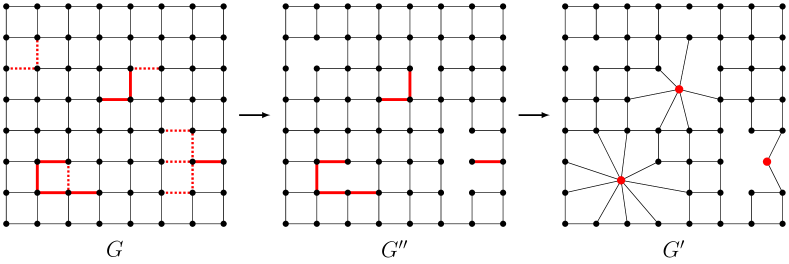
Figure 1. We first perform percolation on $G$ by closing edges with weight outside $[1/A,A]$ (drawn in red). We then condition on the realisation of the uniform spanning tree ${\mathcal{T}}$ on the set of closed (red) edges, with edges in ${\mathcal{T}}$ drawn in thick red lines and edges not in ${\mathcal{T}}$ drawn in dotted red lines. Deleting the dotted red edges leads to the graph $G^{\prime\prime}$, and further contracting the solid red edges leads to the graph $G^{\prime}$.

Given ${\mathcal{T}}(K)$, we define a new graph (which may have multiple edges)

$$G^{\prime}=G^{\prime}(K,{\mathcal{T}}(K)):=\Big{(}G-\big{[}K\backslash{\mathcal{T}}(K)\big{]}\Big{)}/{\mathcal{T}}(K),$$ (3.2)

where edges in $K\backslash{\mathcal{T}}(K)$ are deleted and edges in ${\mathcal{T}}(K)$ are contracted (cf. Section 2.1), see Figure 1. The edge set of $G^{\prime}$ is exactly the set of open edges $E\backslash K$, and we assign to each edge the original corresponding weight in $w$ and call the collection of their weights $w^{\prime}$. The goal of this section is to give a lower bound on the bottleneck ratio $\Phi_{(G^{\prime},w^{\prime})}$ for $(G^{\prime},w^{\prime})$ that is uniform both over the configuration of ${\mathcal{T}}(K)$ and over all $w$ in the high probability event ${\mathcal{B}}:=\bigcap_{i=1}^{4}B_{i}$. This is the event given by the intersection of

$$B_{1} :=\{|V(\mathcal{C}_{1})|\geq 3n/4\},$$ (3.3)

$$B_{2} :=\{h_{\mathcal{C}_{1}}\geq 1/\log n\},$$

$$B_{3} :=\{\text{all connected components of }G\setminus V(\mathcal{C}_{1})\text{ have size at most}\,\log n\},$$

$$B_{4} :=\{\text{the closed edges $K$ form clusters of size at most}\,\log n\},$$

where we recall that $\mathcal{C}_{1}=\mathcal{C}_{1}(p)$ denotes the largest open cluster in the percolation process on $G$ with respect to the edge weights $w$. Lemmas 3.1, 3.2, 3.3 and 3.4 imply that for any $\eta>0$,

$$\mathbb{P}(B_{1}\cap B_{2}\cap B_{3}\cap B_{4})\geq 1-\frac{C}{n^{\eta}},$$ (3.4)

provided that $A$ is chosen large enough so that $p=p(A)=\mu([1/A,A])$ is close enough to $1$.

Proposition 3.5.

Let $G=(V,E)$ be a $b$-expander with $b>0$, $|V|=n$, and maximum degree $\Delta<\infty$. Let $w=(w_{e})_{e\in E}$ be i.i.d. random edge weights with common distribution $\mu$. Given any $\eta>0$, let $A$ be chosen such that (3.4) holds. Let $G^{\prime}=G^{\prime}(K,{\mathcal{T}}(K))$ be defined as in (3.2) with parameter $p(A)$. Then for all $w\in\bigcap_{i=1}^{4}B_{i}$ and for $\boldsymbol{\mathrm{P}}^{w}$-a.e. ${\mathcal{T}}(K)$,

$$\Phi_{(G^{\prime},w^{\prime})}\geq\frac{1}{8A^{2}\Delta^{2}(\log n)^{3}}.$$

Note that although all edges in $G^{\prime}$ are assigned weights in $[1/A,A]$, which makes the bottleneck ratio $\Phi_{(G^{\prime},w^{\prime})}$ comparable to the isoperimetric constant $h_{G^{\prime}}$ of the unweighted graph $G^{\prime}$, the degree of vertices in $G^{\prime}$ can be arbitrarily large due to the contraction of edges. Therefore, to prove Prop. 3.5, we first lower bound the isoperimetric constant $h_{G^{\prime\prime}}$ of the graph

$$G^{\prime\prime}=G^{\prime\prime}(K,{\mathcal{T}}(K)):=G-K\backslash{\mathcal{T}}(K),$$ (3.5)

i.e., the graph obtained by deleting edges in $K\backslash{\mathcal{T}}(K)$, but without contracting edges in ${\mathcal{T}}(K)$, see Figure 1. We then show that contraction will increase the maximal degree by a factor of $\log n$, which decreases the isoperimetric constant by a factor of at most $(\log n)^{c}$.

We have the following lower bound on $h_{G^{\prime\prime}}$.

Lemma 3.6.

Assume the setting as in Proposition 3.5. For all $w\in\bigcap_{i=1}^{4}B_{i}$ and $\boldsymbol{\mathrm{P}}^{w}$-a.e. ${\mathcal{T}}(K)$, we have

$$h_{G^{\prime\prime}}\geq\frac{1}{8\Delta(\log n)^{2}}.$$

Proof.

Fix an arbitrary realisation of ${\mathcal{T}}(K)$ under the law $\boldsymbol{\mathrm{P}}^{w}$, which determines the graph $G^{\prime\prime}$. Let $S\subseteq V$ be any vertex set with $1\leq|S|\leq n/2$, which can be decomposed into $S_{1}:=S\cap V(\mathcal{C}_{1})$ and $S_{2}=S\setminus S_{1}$. Since the event $B_{3}$ occurs, $G\backslash V(\mathcal{C}_{1})$ consists of disconnected components of size at most $\log n$. Let $L_{1},\ldots,L_{M}$ denote the components of $G\backslash V(\mathcal{C}_{1})$ that contain some vertex in $S_{2}$. Then $|S_{2}|\leq M\log n$.

Note that $E(S,S^{c})$ in particular contains all edges in $\mathcal{C}_{1}$ that connect $S_{1}$ to $V(\mathcal{C}_{1})\backslash S_{1}$, which we denote here by $E_{\mathcal{C}_{1}}(S_{1},S_{1}^{c})$. Since the event $B_{2}$ occurs, we can use the isoperimetric constant of $\mathcal{C}_{1}$ to obtain

$$|E_{\mathcal{C}_{1}}(S_{1},S_{1}^{c})| \geq\frac{1}{\log n}\big{(}\mathds{1}_{\{|S_{1}|\leq|V(\mathcal{C}_{1})|/2\}}|S_{1}|+\mathds{1}_{\{|V(\mathcal{C}_{1})|/2<|S_{1}|\leq n/2\}}|V(\mathcal{C}_{1})\backslash S_{1}|\big{)}$$ (3.6)

$$\geq\frac{|S_{1}|}{2\log n},$$

where in the second line we used that, on the event $B_{1}$, the giant component satisfies $|V(\mathcal{C}_{1})|\geq 3n/4$.

To bound $E(S,S^{c})$, we distinguish between two cases. For the case $|S_{1}|\geq\frac{M}{2\Delta}$, we have

$$\frac{|E(S,S^{c})|}{|S|}\geq\frac{|E_{\mathcal{C}_{1}}(S_{1},S_{1}^{c})|}{|S_{1}|+M\log n}\geq\frac{\frac{1}{2\log n}}{1+\frac{M\log n}{|S_{1}|}}\geq\frac{1}{2\log n(1+2\Delta\log n)}\geq\frac{1}{8\Delta(\log n)^{2}},$$

which satisfies the desired bound on $h_{G^{\prime\prime}}$.

We now consider the case $|S_{1}|<\frac{M}{2\Delta}$. Note that regardless of the realisation of ${\mathcal{T}}(K)$, $G^{\prime\prime}$ must remain a connected graph because ${\mathcal{T}}$ connects all vertices in $V$. Therefore, for each $L_{i}$, $1\leq i\leq M$, there is at least one edge in $G^{\prime\prime}$ connecting $L_{i}$ to $\mathcal{C}_{1}$. Since $G^{\prime\prime}$ has maximal degree $\Delta$, each vertex in $V(\mathcal{C}_{1})$ can connect to at most $\Delta$ different $L_{i}$’s. It follows that $S_{1}$ can connect to at most $\Delta|S_{1}|<M/2$ different $L_{i}$’s. Therefore, at least $M/2$ components among $L_{1},\ldots,L_{M}$ are connected to some vertex in $V(\mathcal{C}_{1})\backslash S_{1}$, and hence $E(S,S^{c})\geq M/2$. It follows that

$$\frac{|E(S,S^{c})|}{|S|}\geq\frac{M/2}{|S_{1}|+M\log n}\geq\frac{M/2}{\frac{M}{2\Delta}+M\log n}\geq\frac{1}{1+2\log n},$$

which also satisfies the desired bound on $h_{G^{\prime\prime}}$.

Since the above bounds hold for all $S\subset V$ with $1\leq|S|\leq n/2$ and are uniform in the realisation of ${\mathcal{T}}(K)$, Lemma 3.6 follows. ∎

We are now ready to prove Prop. 3.5.

Proof of Proposition 3.5.

Fix an arbitrary realisation of ${\mathcal{T}}(K)$ under the law $\boldsymbol{\mathrm{P}}^{w}$, which determines the graphs $G^{\prime\prime}$ and $G^{\prime}$. Recall that $G^{\prime}$ is constructed from $G^{\prime\prime}$ by contracting all edges in ${\mathcal{T}}(K)$, which is equivalent to contracting each connected component in the forest ${\mathcal{T}}(K)$ into a single vertex. On the event $B_{4}$, these closed clusters have size at most $\log n$. Since $G^{\prime\prime}$ has maximum degree $\Delta$, after contraction, $G^{\prime}$ has maximum degree at most $\Delta\log n$.

Let $S\subset V(G^{\prime})$, and let $\tilde{S}\subset V(G^{\prime\prime})$ be the pre-image of $S$ under the contraction that generates $G^{\prime}$ from $G^{\prime\prime}$. On the event $\bigcap_{i=1}^{4}B_{i}$, it holds that $h_{G^{\prime\prime}}\geq 1/8\Delta(\log n)^{2}$ by Lemma 3.6. We then have

$$|E_{G^{\prime}}(S,S^{c})|=|E_{G^{\prime\prime}}(\tilde{S},\tilde{S}^{c})|\geq\frac{1}{8\Delta(\log n)^{2}}\min\{|\tilde{S}|,|\tilde{S}^{c}|\},$$ (3.7)

where $E_{G^{\prime}}(S,S^{c})$ denotes the set of edges in $G^{\prime}$ connecting $S$ and $S^{c}$. To lower bound the bottleneck ratio $\Phi_{(G^{\prime},w^{\prime})}$ for the weighted graph $(G^{\prime},w^{\prime})$, note that

$$\sum_{e\in E_{G^{\prime}}(S,S^{c})}w_{e}\geq\frac{1}{A}\,|E_{G^{\prime}}(S,S^{c})|,$$

since all edges in $G^{\prime\prime}$, and hence $G^{\prime}$, have weights in $[1/A,A]$. On the other hand, for $S^{\prime}=S$ or $S^{c}$, because vertices in $G^{\prime}$ have degree at most $\Delta\log n$, we have

$$\sum_{x\in S^{\prime},y\in V(G^{\prime})}w_{\{x,y\}}\leq A\Delta\log n\cdot|S^{\prime}|\leq A\Delta\log n\cdot|\tilde{S}^{\prime}|\,.$$

Together with (3.7), this implies that, for all $S\subset V(G^{\prime})$,

$$\sum_{e\in E_{G^{\prime}}(S,S^{c})}w_{e}\geq\frac{1}{8A^{2}\Delta^{2}(\log n)^{3}}\min\Big{\{}\sum_{x\in S,y\in V(G^{\prime})}w_{\{x,y\}},\sum_{x\in S^{c},y\in V(G^{\prime})}w_{\{x,y\}}\Big{\}}.$$

By (2.5), this implies $\Phi_{(G^{\prime},w^{\prime})}\geq\frac{1}{8A^{2}\Delta^{2}(\log n)^{3}}$. ∎

4. Proof of Theorem 1.1 for Expanders

We follow the same notation as in Section 3.3, where, given the edge weights $w=(w_{e})_{e\in E}$, an edge $e$ is open if $w_{e}\in[1/A,A]$ and closed otherwise. The set of closed edges is denoted by $K$. Let $A$ be chosen as in Proposition 3.5 such that the events $(B_{i})_{1\leq i\leq 4}$ defined in (3.3) hold jointly with probability at least $1-C/n^{\eta}$ for some $\eta>0$ that can be chosen arbitrarily. From now on we will assume $w\in\bigcap_{i=1}^{4}B_{i}$, provided $\gamma$ in Theorem 1.1 is chosen to satisfy $\gamma<\eta$.

Given $w$, and for any realisation of ${\mathcal{T}}(K)$ under $\boldsymbol{\mathrm{P}}^{w}$, let $(G^{\prime},w^{\prime})$ be defined as in (3.2). Let $V(G^{\prime})$ and $E(G^{\prime})$ denote the vertex and edge set of $G^{\prime}$. By Proposition 3.5, we have

$$\Phi_{(G^{\prime},w^{\prime})}\geq\frac{1}{8A^{2}\Delta^{2}(\log n)^{3}}$$ (4.1)

uniformly in $w\in\bigcap_{i=1}^{4}B_{i}$ and for $\boldsymbol{\mathrm{P}}^{w}$-a.e. ${\mathcal{T}}(K)$.

We will now apply Theorem 2.3 to $(G^{\prime},w^{\prime})$. Let us define the quantities $D,\alpha,\vartheta$ involved in conditions (2.10), (2.11) and (2.12):

• Condition (2.10): since the vertices in $G^{\prime}$ have degree at most $\Delta\log n$ as noted in the proof of Proposition 3.5, and the edge weights all lie in $[1/A,A]$, it is clear that we can take $D:=\Delta A^{2}\log n$.

• Condition (2.11): if $\pi$ denotes the stationary distribution of the lazy random walk on $(G^{\prime},w^{\prime})$, then

  $$\pi_{\rm min}=\min_{v\in V(G^{\prime})}\pi(v)\geq\frac{1}{|V(G^{\prime})|}\frac{\frac{1}{A}}{\Delta A\log n}\geq\frac{1}{\Delta A^{2}n\log n}.$$

  Then Theorem 2.2 and (4.1) together imply

  $$t_{\text{mix}}(G^{\prime},w^{\prime})\leq C(A,\Delta)(\log n)^{7}$$

  for some constant $C(A,\Delta)$ depending only on $A$ and $\Delta$. Therefore, we may choose any $\alpha\in(0,1/2)$.

• Condition (2.12): to identify $\vartheta$ we use the trivial bound

  $$\sum_{t=0}^{t_{\text{mix}}(G^{\prime},w^{\prime})}(t+1)\sup_{v\in V(G^{\prime})}q_{t}(v,v)\leq(t_{\text{mix}}(G^{\prime},w^{\prime})+1)^{2}\leq(C(A,\Delta)+1)^{2}(\log n)^{14}=:\vartheta\,.$$ (4.2)

Denote now $m:=|V(G^{\prime})|$, which, thanks to the event $B_{4}$, satisfies $n/\log n\leq m\leq n$. Since the above choices of $D,\alpha,\vartheta$ are uniform for $\boldsymbol{\mathrm{P}}^{w}$-a.e. ${\mathcal{T}}(K)$, Theorem 2.3 implies that there exist $\gamma^{\prime}\in(0,\eta)$, $c_{1}=c_{1}(A,\Delta)$ and $c_{2}$ such that for large enough $n$ and any $\varepsilon>n^{-\gamma^{\prime}}$,

$$\boldsymbol{\mathrm{P}}^{w}\Big{(}\frac{\sqrt{m}}{(c_{1}\varepsilon^{-1}\log n)^{c_{2}}}\leq diam({\mathcal{T}}_{(G^{\prime},w^{\prime})})\leq\sqrt{m}(c_{1}\varepsilon^{-1}\log n)^{c_{2}}\Big{)}\geq 1-\varepsilon\,.$$ (4.3)

This bound is uniform for $w\in\bigcap_{i=1}^{4}B_{i}$, and the complement of this event has probability at most $n^{-\eta}\ll\varepsilon$. To conclude the proof of Theorem 1.1, it only remains to translate the bounds on $diam({\mathcal{T}}_{(G^{\prime},w^{\prime})})$ into bounds on $diam({\mathcal{T}}_{(G,w)})$.

By the spatial Markov property in Lemma 2.1, we can couple ${\mathcal{T}}={\mathcal{T}}_{(G,w)}$ and ${\mathcal{T}}_{(G^{\prime},w^{\prime})}$ such that ${\mathcal{T}}={\mathcal{T}}_{(G^{\prime},w^{\prime})}\cup{\mathcal{T}}(K)$. To recover ${\mathcal{T}}$ from ${\mathcal{T}}_{(G^{\prime},w^{\prime})}$, we need to undo the contraction of edges in ${\mathcal{T}}(K)\subset K$, which consists of disjoint trees of size at most $\log n$. Since the contraction of these trees in ${\mathcal{T}}$ into single vertices decreases the length of paths in ${\mathcal{T}}$, we have $diam({\mathcal{T}}_{(G^{\prime},w^{\prime})})\leq diam({\mathcal{T}})$. In the other direction, when we take a path in ${\mathcal{T}}_{(G^{\prime},w^{\prime})}$ and undo the contraction, the worst case is when each vertex along the path is replaced by a path of length $\log n$, so $diam({\mathcal{T}})\leq\log n\cdot diam({\mathcal{T}}_{(G^{\prime},w^{\prime})})$. These bounds and the fact that $n/\log n\leq m\leq n$ readily imply Theorem 1.1, where we can pick $0<\gamma\leq\gamma^{\prime}$ and $c>0$ large enough to also absorb the factor $c_{1}$.

Remark 4.1.

Notice that in (4.3) the exponent of the $\log n$ corrections is independent of $b$, $\Delta$ and $\mu$, cf. Remark 1.2, and $\gamma$ can be taken independent of all parameters. In fact, we only impose $\gamma<\eta$, for an arbitrary large $\eta$, and $\gamma$ less than a small constant times $\alpha$ (see Appendix A), where $\alpha$ can be chosen to be anything below $1/2$.

5. Finite Boxes in $\mathbb{Z}^{d}$

Consider the lattice $\mathbb{Z}^{d}$ with edge set $E^{d}:=\{\{x,y\}:x,y\in\mathbb{Z}^{d},\|x-y\|_{1}=1\}$. For integers $L\geq 1$, consider the induced graph $G_{n}$ with $n=(2L+1)^{d}$ many vertices, defined by taking the vertex set $V_{n}=\mathbb{Z}^{d}\cap[-L,L]^{d}$. For notational sake, we shall sometimes drop the subscript $n$. To bound the diameter of the UST on $G_{n}$ with random edge weights, we will follow the same strategy as for expander graphs in Sections 3 and 4. The key difference is that for finite boxes in $\mathbb{Z}^{d}$ with $n$ vertices, it is known that the mixing time is of order $n^{2/d}$ (see e.g. [12, Theorem 1.1]). Therefore, when we bound the parameter $\vartheta$ in (2.12) for the graph $(G^{\prime},w^{\prime})$ (recall from Section 3.3), we can no longer apply the crude bound

$$\sum_{t=0}^{t_{\text{mix}}}(t+1)\sup_{v\in V}q_{t}(v,v)\leq(t_{\text{mix}}+1)^{2}$$

as we did in (4.2) for expander graphs. Instead, we need to apply sharper bounds on the lazy random walk transition kernel $q_{t}(\cdot,\cdot)$. This will be achieved by replacing the notion of bottleneck ratio $\Phi_{(G,w)}$ in (2.4) with the notion of bottleneck profile $\Phi_{(G,w)}(r)$ in (5.1) below.

5.1. Heat kernel estimates

For a finite connected weighted graph $(G,w)$, let $\pi$ denote the stationary distribution of the lazy random walk on $(G,w)$ defined as in (2.6), and let $\pi_{\min}:=\min_{v\in V}\pi(v)$. Recall from (2.8) that for non-empty $S\subset V$, $\Phi_{(G,w)}(S)=\frac{1}{\pi(S)}\sum_{x\in S,y\in S^{c}}\pi(x)q(x,y)$. We then define the bottleneck profile by

$$\Phi_{(G,w)}(r):=\left\{\begin{aligned} \min\limits_{0<\pi(S)\leq r}\Phi_{(G,w)}(S)&\qquad\mbox{if }\pi_{\rm min}\leq r\leq 1/2,\\ \Phi_{(G,w)}(1/2)\qquad&\qquad\mbox{if }r>1/2.\end{aligned}\right.$$ (5.1)

Note that $\Phi_{(G,w)}(r)$ is decreasing in $r$, and $\Phi_{(G,w)}(1/2)=\Phi_{(G,w)}$, the bottleneck ratio defined in (2.4). We will need the following result from [23], which can be thought of as a strengthening of the upper bound on the mixing time in Theorem 2.2.

Theorem 5.1 (Theorem 1 in [23]).

Let $u,v\in V(G)$, and let $(q_{t}(u,v))_{t\geq 0}$ be the transition kernel of the lazy random walk on $(G,w)$. If

$$t\geq 1+\int_{4\min\{\pi(u),\pi(v)\}}^{\frac{4}{\xi}}\frac{4}{r\Phi_{(G,w)}^{2}(r)}dr,$$

then

$$\Big{|}\frac{q_{t}(u,v)}{\pi(v)}-1\Big{|}\leq\xi\,.$$

We note that the above result also gives a bound on the mixing time. For our purposes, we will only use it to bound $q_{t}(v,v)$ by choosing an appropriate $\xi=\xi(t)$.

Let $G=(V,E)$ be the box $[-L,L]^{d}\cap\mathbb{Z}^{d}$ with $n$ vertices, and let $w=(w_{e})_{e\in E}$ be i.i.d. edge weights as in Theorem 1.1. Let $(G^{\prime},w^{\prime})$ be defined as in (3.2), which is obtained from $(G,w)$ by conditioning on ${\mathcal{T}}(K)$, the UST on $(G,w)$ restricted to edges $e\in E$ with $w_{e}\notin[1/A,A]$, which are called closed edges in a percolation process with parameter $p=p(A)=\mu([1/A,A])$. To prove Theorem 1.1 for finite boxes on $\mathbb{Z}^{d}$ with $d\geq 5$, the main technical ingredient is the following bound on the bottleneck profile for $(G^{\prime},w^{\prime})$.

Lemma 5.2.

Let $\eta>0$. There exist constants $C=C(d,\eta)>0$ and $p^{*}=p^{*}(d,\eta)<1$ such that if $p(A)>p^{*}$, then there is an event $\tilde{\mathcal{B}}$ (see (5.4) below) with $\mathbb{P}(w\in\tilde{\mathcal{B}})\geq 1-n^{-\eta}$ such that if $w\in\tilde{\mathcal{B}}$, then for $\boldsymbol{\mathrm{P}}^{w}$-a.e. ${\mathcal{T}}(K)$ and any $r\geq\pi_{\rm min}$, we have

$$\Phi_{(G^{\prime},w^{\prime})}(r)\geq\frac{C}{A^{4}(\log n)^{d+4}}\Big{(}\frac{\pi_{\rm min}}{r}\Big{)}^{1/d}.$$

We will postpone the proof of Lemma 5.2 to Section 5.2.

Proof of Theorem 1.1 for finite boxes in $\mathbb{Z}^{d}$.

Let $G=(V,E)$ be the box $[-L,L]^{d}\cap\mathbb{Z}^{d}$ with $n$ vertices, and let $w=(w_{e})_{e\in E}$ be i.i.d. edge weights with common distribution $\mu$. We proceed as in the proof of Theorem 1.1 for expander graphs in Section 4. As in Section 3.3, we couple the edge weights $w=(w_{e})_{e\in E}$ to a percolation process with parameter $p=p(A)=\mu([1/A,A])$, and let $(G^{\prime},w^{\prime})$ be defined from $(G,w)$ as in (3.2). We will again verify the three conditions of Theorem 2.3 for $(G^{\prime},w^{\prime})$. In what follows, $\eta>0$ can be chosen arbitrarily, and $C$ denotes a generic constant depending only on $d$ and $\eta$, whose precise value may change from line to line.

• Condition (2.10): The maximum degree in $G$ is $2d$, and hence by Lemma 3.2, we can choose $A$ large enough such that with probability at least $1-n^{-\eta}$, every cluster of closed edges is of size at most $\log n$. Following the notation in (3.3), we denote the set of such edge weights configurations by $\tilde{B}_{4}$. Then for $w\in\tilde{B}_{4}$, $(G^{\prime},w^{\prime})$ satisfies condition (2.10) with $D=2dA^{2}\log n$.

• Condition (2.11): For $w\in\tilde{B}_{4}$, the stationary distribution of the lazy random walk on $(G^{\prime},w^{\prime})$ satisfies

  $$\frac{1}{nD}=\frac{1}{2dA^{2}n\log n}\leq\pi_{\rm min}\leq\pi_{\rm max}\leq\frac{D}{n}=\frac{2dA^{2}\log n}{n}.$$ (5.2)

  Using Lemma 5.2 with $r=1/2$ and Theorem 2.2 gives

  $$t_{\text{mix}}(G^{\prime},w^{\prime})\leq CA^{8}(\log n)^{2d+8}\pi_{\rm min}^{-2/d}\log(\pi_{\rm min}^{-1})\leq CA^{8+4/d+1}(\log n)^{2d+8+2/d+1}n^{2/d}\,.$$ (5.3)

  Since $d\geq 5$, condition (2.11) is satisfied for some $\alpha>0$.

• Condition (2.12): Let $w\in\tilde{\mathcal{B}}$ for the event $\tilde{\mathcal{B}}$ in Lemma 5.2, and let

  $$\xi=\xi(t)=C_{1}A^{4d}(\log n)^{d(d+4)}\pi_{\rm min}^{-1}(t-1)^{-d/2}$$

  for some large $C_{1}$ to be determined later. For small $t\geq 2$ that satisfies $\pi(v)\geq\xi(t)^{-1}$, we use the trivial bound $q_{t}(v,v)\leq 1\leq(\xi(t)+1)\pi(v)$. To bound $q_{t}(v,v)$ for larger $t$ with $\pi(v)<\xi(t)^{-1}$, we use the bound from Lemma 5.2

  $$1+\int_{4\pi(v)}^{\frac{4}{\xi}}\frac{4}{r\Phi_{(G^{\prime},w^{\prime})}^{2}(r)}dr \leq 1+CA^{8}(\log n)^{2d+8}\pi_{\rm\min}^{-2/d}\int_{4\pi(v)}^{\frac{4}{\xi}}r^{2/d-1}dr$$

  $$\leq 1+CA^{8}(\log n)^{2d+8}\pi_{\rm\min}^{-2/d}\xi^{-\frac{2}{d}}$$

  $$=1+C\cdot C_{1}^{-2/d}(t-1)\leq t\,,$$

  where we choose $C_{1}$ large enough so that the last inequality is satisfied. Then by Theorem 5.1 for $t\geq 2$,

  $$q_{t}(v,v) \leq(\xi+1)\pi(v)\leq C_{1}A^{4d}(\log n)^{d(d+4)}(t-1)^{-d/2}\frac{\pi_{\rm max}}{\pi_{\rm min}}+\pi(v)$$

  $$\leq CA^{4d+2}(\log n)^{d(d+4)+1}t^{-d/2}+\pi(v)\,.$$

  Using the above, we may bound

  $$\sum_{t=0}^{t_{\text{mix}}(G^{\prime},w^{\prime})}(t+1)\sup_{v\in V(G^{\prime})}q_{t}(v,v) \leq CA^{4d+2}(\log n)^{d(d+4)+1}\sum_{t=0}^{\infty}(t+1)t^{-d/2}+(t_{\text{mix}}+1)^{2}\pi_{\rm\max}$$

  $$\leq CA^{4d+2}(\log n)^{d(d+4)+1}+CA^{20+8/d}(\log n)^{4d+4/d+19}n^{4/d-1},$$

  where we used (5.2) and (5.3). Therefore, for $w\in\tilde{B}_{4}\cap\tilde{\mathcal{B}}$, the escaping condition (2.12) is satisfied with $\vartheta=c_{1}(\log n)^{c_{2}}$ for some $c_{1}=c_{1}(A,d)$ depending on $d$, $\mu$ and $\eta$, and some $c_{2}=c_{2}(d)$ that depends only on $d$.

We may thus apply Theorem 2.3 to $(G^{\prime},w^{\prime})$ to obtain bounds on the diameter of the UST on $(G^{\prime},w^{\prime})$. Deducing bounds on the diameter of the UST on $(G,w)$ then follows exactly as in Section 4 for expander graphs. ∎

Remark 5.3.

In the above proof, the exponent of the $\log n$ correction term depends on $d$ but not on the edge weight distribution $\mu$. Furthermore, for the same reasons as in Remark 4.1, $\gamma$ can be taken as a universal constant as $\alpha$ can be chosen as anything below $1/10\leq 1/2-2/d$ for all $d\geq 5$.

5.2. Proof of Lemma 5.2

Similar to the proof of Proposition 3.5 for expander graphs, we will show that the bottleneck profile of $(G^{\prime},w^{\prime})$ differs from the bottleneck profile of the largest percolation cluster $\mathcal{C}_{1}$ only by a polylogarithmic factor. To this end, we define the following analogues of the events $B_{1},B_{2},B_{3}$ and $B_{4}$ in (3.3) for finite boxes in $\mathbb{Z}^{d}$, where $c_{0}$ is given in Lemma 5.6 below:

$$\tilde{B}_{1} :=\{|V(\mathcal{C}_{1}(p))|\geq 3n/4\},$$ (5.4)

$$\tilde{B}_{2} :=\{\forall S\subseteq\mathcal{C}_{1}\;\text{with}\,(\log n)^{\frac{d^{2}}{d-1}}\leq|S|\leq\frac{|V(\mathcal{C}_{1})|}{2},|E_{\mathcal{C}_{1}}(S,S^{c})|\geq c_{0}|S|^{\frac{d-1}{d}}\},$$

$$\tilde{B}_{3} :=\{\text{all connected components of }G\setminus V(\mathcal{C}_{1})\text{ have size at most}\,(\log n)^{\frac{d}{d-1}}\},$$

$$\tilde{B}_{4} :=\{\text{the closed edges in $K$ form clusters of size at most}\,\log n\},$$

where ${\mathcal{C}}_{1}$ denotes the largest percolation cluster in $G$ for the percolation process coupled to $w$ such that $e$ is open if $w_{e}\in[1/A,A]$, and $E_{\mathcal{C}_{1}}(S,S^{c})$ denotes the set of edges between $S\subset V(\mathcal{C}_{1})$ and $S^{c}=V(\mathcal{C}_{1})\backslash S$ in the graph $\mathcal{C}_{1}$. We denote by $p=p(A)=\mu([1/A,A])$ the percolation parameter.

As noted before, by Lemma 3.2, for any $\eta>0$ we can choose $A$ large enough such that $\mathbb{P}(w\in\tilde{B}_{4})\geq 1-Cn^{-\eta}$. The following lemma gives a similar bound for $\mathbb{P}(w\in\tilde{B}_{1})$.

Lemma 5.4.

There exist $p^{*}_{1}=p^{*}_{1}(d)\in(0,1)$ and constants $c,C>0$ such that for all $p\in(p^{*}_{1},1]$ and $n\in\mathbb{N}$,

$$\mathbb{P}\Big{(}|V(\mathcal{C}_{1}(p))|<\frac{3n}{4}\Big{)}\leq C{\rm e}^{-cn^{1/d}}$$ (5.5)

Proof.

This follows from Theorem 1.2 of [15] by choosing $\varepsilon=1/4$. ∎

The next lemma gives the desired bound for $\mathbb{P}(w\in\tilde{B}_{3})$.

Lemma 5.5.

For any $\eta>0$, there exist $p^{*}_{2}=p^{*}_{2}(d,\eta)\in(0,1)$ and constant $C>0$ such that for all $p\in(p^{*}_{2},1]$ and $n\in\mathbb{N}$,

$$\mathbb{P}\big{(}\exists\text{ a connected component }H\subseteq G\backslash V(\mathcal{C}_{1}(p))\text{ with }|H|\geq(\log n)^{\frac{d}{d-1}}\big{)}\leq\frac{C}{n^{\eta}}.$$ (5.6)

Proof.

We follow the proof of [27, Lemma 3.2], which treats a similar event on the torus $\mathbb{T}^{d}$. By Lemma 5.4, we may first restrict to the event $\{|\mathcal{C}_{1}(p)|\geq\frac{3n}{4}\}$. We will then bound the probability in (5.6) by a union bound over all $H\subset V$ in the box $G=(V,E)$ that can arise as a connected component of $G\backslash V(\mathcal{C}_{1}(p))$ with $(\log n)^{\frac{d}{d-1}}\leq|H|\leq\frac{n}{4}$. Equivalently, we can take the union bound over all realisations of the edge boundary set $\partial H\subset E$, where each edge in $\partial H$ must be closed in the percolation configuration for $H$ to be a connected component of $G\backslash V(\mathcal{C}_{1}(p))$. By the edge isoperimetric inequality for finite boxes in [13, Theorem 3], for $|H|$ with $|H|\leq n/2$, we have

$$|\partial H|\geq\min\{|H|^{1-\frac{1}{r}}rn^{\frac{1}{r}-\frac{1}{d}}:r=1,2,\ldots,d\}\geq|H|^{\frac{d-1}{d}}.$$ (5.7)

Since we will only consider $H$ with $|H|\geq(\log n)^{\frac{d}{d-1}}$, this imposes the constraint that

$$|\partial H|\geq\log n.$$ (5.8)

We say that two edges $e,f\in E$ are $*$-connected if one of the two endpoints of $e$ is within $\ell_{\infty}$-distance $1$ of one of the two endpoints of $f$. Then, for $H\subset V$ to arise as a connected component of $G\backslash V(\mathcal{C}_{1}(p))$, we note that $\partial H$ must be a $*$-connected set of edges. Further note that, if we regard the edges in $E$ as vertices of a new graph, whose edge set consists of pairs of edges in $E$ that are $*$-connected, then this new graph has at most $2dn$ vertices with maximum degree bounded by $8d^{2}$. As cited in the proof of Lemma 3.2, the number of $*$-connected $\partial H\subset E$ with $|\partial H|=k$ is then bounded by $\frac{n}{k}(8d^{2}{\rm e})^{k}$.

We can now first apply Lemma 5.4 and then take a union bound over all $*$-connected edge sets $\partial H\subset E$ with $|\partial H|\geq\log n$ to bound the probability in (5.6) by

$$C{\rm e}^{-cn^{1/d}}+\sum_{k=\log n}^{2dn}\frac{n}{k}(8d^{2}{\rm e})^{k}(1-p)^{k}\leq\frac{C}{n^{\eta}},$$

where the last bound holds uniformly in $p>p_{2}^{*}$ if $p_{2}^{*}$ is sufficiently close to $1$. ∎

Lastly, the following lemma gives the desired bound for $\mathbb{P}(w\in\tilde{B}_{2})$.

Lemma 5.6.

There exists $c_{0}\in(0,1)$ such that for any $\eta>0$, there exist $p_{3}^{*}=p_{3}^{*}(d,\eta)\in(0,1)$ and $C>0$, and for all $p\in(p_{3}^{*},1]$ and $n\in\mathbb{N}$, we have

$$\mathbb{P}\Big{(}\exists S\subseteq V(\mathcal{C}_{1}(p))\,:(\log n)^{\frac{d^{2}}{d-1}}\leq|S|\leq\frac{|V(\mathcal{C}_{1}(p))|}{2},|E_{\mathcal{C}_{1}}(S,S^{c})|\leq c_{0}|S|^{\frac{d-1}{d}}\Big{)}\leq\frac{C}{n^{\eta}}.$$ (5.9)

Proof sketch..

We can follow the arguments in [12]. First we can prove a variant of (5.9) where $S$ is further required to satisfy the condition that both $S$ and $S^{c}:=V(\mathcal{C}_{1})\backslash S$ are connected in $\mathcal{C}_{1}$, that is, for $p$ close enough to $1$,

$$\mathbb{P}\Big{(}\exists\text{connected }S\subseteq V(\mathcal{C}_{1}(p))\, :V(\mathcal{C}_{1}(p))\setminus S\text{ is connected in }\mathcal{C}_{1}(p),$$ (5.10)

$$(\log n)^{\frac{d}{d-1}}\leq|S|\leq\frac{|V(\mathcal{C}_{1}(p))|}{2},|E_{\mathcal{C}_{1}}(S,S^{c})|\leq\frac{1}{2}|S|^{\frac{d-1}{d}}\Big{)}\leq\frac{C}{n^{\eta}}.$$

This is essentially [12, Theorem 2.4] (or [26, Corollary 1.4]) with a quantitative probability bound. Following the proof in [12, Section 2.4], the basic observation is that for any subset $S$ of the box $G=(V,E)$ with $|S|\geq(\log n)^{\frac{d}{d-1}}$, if $S$ turns out to be a connected subset of $\mathcal{C}_{1}$ such that $S^{c}$ is also connected in $\mathcal{C}_{1}$ , then $S^{c}$ must lie in one of the connected components of $V\backslash S$ in $G$ (denoted by $A_{r}$ in [12, Section 2.4]). By the assumption $|S|\leq\frac{1}{2}|V(\mathcal{C}_{1})|$, we have $|S|\leq|A_{r}|$, and hence by the isoperimetric inequality (5.7), the number of edges between $S$ and $A_{r}$ in $G$ is bounded by

$$|E_{G}(S,A_{r})|\geq|S|^{\frac{d-1}{d}}\geq\log n.$$

Since we are assuming $S\subseteq V(\mathcal{C}_{1})$, for the event $\{|E_{\mathcal{C}_{1}}(S,S^{c})|\leq\frac{1}{2}|S|^{\frac{d-1}{d}}\}$ to occur, at least half of the edges in $E_{G}(S,A_{r})$ must be closed in the percolation configuration, the probability of which can be bounded by ${\rm e}^{-c|E_{G}(S,A_{r})|}$ for an arbitrarily large $c$ if $p$ is chosen close enough to $1$. Taking a union bound over all possible choices of $E_{G}(S,A_{r})$ with $|E_{G}(S,A_{r})|\geq\log n$ then gives the desired probability bound of $C/n^{\eta}$ if $p$ is chosen close enough to $1$, since $E_{G}(S,A_{r})$ is a so-called minimal cut set, and the number of minimal cut sets in $G$ with cardinality $m$ is bounded by $n\tilde{c}^{m}$ for some $\tilde{c}$ depending only on $d$. For the remainder of the proof we assume $p$ is so large such that (5.10) holds.

To extend the bound (5.10) to connected $S$ (without assuming $S^{c}$ is also connected in $\mathcal{C}_{1}$), following the proof of Lemma 2.6 in [12], the key observation is that (cf. [12, Lemma 2.5] and [5, Lemma 4.36]) is that there exists a constant $c_{d}$ depending only on $d$ such that for any $x\in(0,1/2]$, there exists a connected set $A\subset V(\mathcal{C}_{1})$ with $|A|\leq x|V(\mathcal{C}_{1})|$ such that

$$\tilde{\varphi}(x):=\inf_{S\subset V(\mathcal{C}_{1}),|S|\leq x|V(\mathcal{C}_{1})|}\frac{|E_{\mathcal{C}_{1}}(S,S^{c})|}{|S|}\geq c_{d}\frac{|E_{\mathcal{C}_{1}}(A,A^{c})|}{|A|}=:c_{d}\tilde{\varphi}_{A}.$$ (5.11)

Note that our definition of $\tilde{\varphi}$ differs slightly from the definition of $\varphi$ in [12], although they are within constant multiples of each other, which explains the inequality and the constant $c_{d}$ in (5.11). Furthermore, if $x=1/2$, we can choose $A$ in (5.11) such that $A$ and $V(\mathcal{C}_{1})\backslash A$ are both connected in $\mathcal{C}_{1}$. This last fact together with (5.10) (assuming $|V(\mathcal{C}_{1})|\geq 3n/4$, which we may thanks to Lemma 5.4), and the crude bound $\tilde{\varphi}_{A}\geq\frac{1}{|A|}$ for $|A|\leq(\log n)^{\frac{d}{d-1}}$ imply that

$$\mathbb{P}(\tilde{\varphi}(1/2)\geq cn^{-\frac{1}{d}})\geq 1-\frac{C}{n^{\eta}}$$

for some $c>0$ depending on $d$. On the event $\{\tilde{\varphi}(1/2)\geq cn^{-1/d}\}$, we note that for all $S$ with $q|V(\mathcal{C}_{1})|\leq|S|\leq\frac{1}{2}|V(\mathcal{C}_{1})|$ for some fixed $0<q\leq\frac{1}{2}$ to be chosen later, we have

$$\frac{|E_{\mathcal{C}_{1}}(S,S^{c})|}{|S|}\geq\frac{c}{n^{1/d}}\quad\Rightarrow\quad|E_{\mathcal{C}_{1}}(S,S^{c})|\geq c^{\prime}|S|^{\frac{d-1}{d}},$$ (5.12)

where $c^{\prime}$ depends on $d$ and $q$. This implies that (5.9) holds with $c_{0}:=c^{\prime}$ if we restrict to $S\subset V(\mathcal{C}_{1})$ with $q|V(\mathcal{C}_{1})|\leq|S|\leq|V(\mathcal{C}_{1})|/2$.

To show that (5.9) still holds if we restrict to $S\subset V(\mathcal{C}_{1})$ with $(\log n)^{\frac{d^{2}}{d-1}}\leq|S|\leq q|V(\mathcal{C}_{1})|$, we can apply (5.11) to find a connected $A\subset V(\mathcal{C}_{1})$ with $|A|\leq|S|$ such that $\tilde{\varphi}_{S}\geq c_{d}\tilde{\varphi}_{A}$, which implies that

$$\frac{|E_{\mathcal{C}_{1}}(S,S^{c})|}{|S|^{\frac{d-1}{d}}}=\tilde{\varphi}_{S}|S|^{1/d}\geq c_{d}\tilde{\varphi}_{A}|A|^{1/d}=c_{d}\frac{|E_{\mathcal{C}_{1}}(A,A^{c})|}{|A|^{\frac{d-1}{d}}}.$$ (5.13)

We now consider the following two cases (to take into account case (1), which was not addressed in the proof of [12, Lemma 2.6], we need to impose in (5.9) the condition $|S|\geq(\log n)^{d^{2}/(d-1)}$ instead of $|S|\geq(\log n)^{\frac{d}{d-1}}$).

1. If $|A|<(\log n)^{\frac{d}{d-1}}$, then the trivial bound $|E_{\mathcal{C}_{1}}(A,A^{c})|\geq 1$ and $\tilde{\varphi}_{S}\geq c_{d}\tilde{\varphi}_{A}$ gives

   $$\frac{|E_{\mathcal{C}_{1}}(S,S^{c})|}{|S|^{\frac{d-1}{d}}}\geq\frac{c_{d}}{|A|}\cdot|S|^{\frac{1}{d}}\geq c_{d}.$$ (5.14)

2. If $|A|\geq(\log n)^{\frac{d}{d-1}}$, then following the proof of Lemma 2.6 in [12], for $q\in(0,1/2)$ small enough, we can find another connected set $A^{\prime}$ with $V(\mathcal{C}_{1})\backslash A^{\prime}$ also connected in $\mathcal{C}_{1}$ and $|A|\leq|A^{\prime}|\leq|V(\mathcal{C}_{1})|/2$, such that

   $$\frac{|E_{\mathcal{C}_{1}}(A,A^{c})|}{|A|^{\frac{d-1}{d}}}\geq\frac{|E_{\mathcal{C}_{1}}(A^{\prime},(A^{\prime})^{c})|}{|A^{\prime}|^{\frac{d-1}{d}}}\geq\frac{1}{2},$$

   where by (5.10), the last inequality holds on an event with probability at least $1-C/n^{\eta}$. On the same event, by (5.13), we have

   $$\frac{|E_{\mathcal{C}_{1}}(S,S^{c})|}{|S|^{\frac{d-1}{d}}}\geq\frac{c_{d}}{2}.$$ (5.15)

Combining (5.12), (5.14) and (5.15) then gives (5.9) with $c_{0}:=\min\{c^{\prime},c_{d}/2\}$. ∎

We are now ready to prove Lemma 5.2 along the same lines as in the proof of Lemma 3.6 and Proposition 3.5 for expander graphs.

Proof of Lemma 5.2.

Let $(\tilde{B}_{i})_{1\leq i\leq 4}$ be defined as in (5.4), and let $\tilde{\mathcal{B}}:=\cap_{i=1}^{4}\tilde{B}_{i}$. By Lemmas 3.2, 5.4 and 5.5 and Lemma 5.6, for any $\eta>0$, we can choose $A$ (and thus $p=p(A)$) large enough such that

$$\mathbb{P}(\tilde{\mathcal{B}})\geq 1-\frac{C}{n^{\eta}}$$

uniformly in $n$. We will assume the edge weights $w$ are in $\tilde{\mathcal{B}}$ from now on.

As in Section 3.3, let ${\mathcal{T}}(K)$ be any realisation of the uniform spanning tree ${\mathcal{T}}={\mathcal{T}}_{(G,w)}$ restricted to the set of closed edges $K$, and we condition on this realisation. Recall from (3.2) and (3.5) that $G^{\prime\prime}$ is the graph obtained by removing edges in $K$ that are not in ${\mathcal{T}}(K)$, while $G^{\prime}$ is obtained by contracting edges in $G^{\prime\prime}$ that are in ${\mathcal{T}}(K)$.

First, we will show that for any $S\subset V(G^{\prime\prime})$ with $1\leq|S|\leq n/2$, we have

$$|E_{G^{\prime\prime}}(S,S^{c})|\geq\frac{c}{(\log n)^{d+1}}|S|^{\frac{d-1}{d}},$$ (5.16)

for some constant $c>0$ independent of $n$ and ${\mathcal{T}}(K)$. As in the proof of Lemma 3.6, let $S_{1}=S\cap V(\mathcal{C}_{1})$ and $S_{2}=S\setminus S_{1}$, and let $L_{1},\ldots,L_{M}$ denote the components of $G\backslash V(\mathcal{C}_{1})$ that contain some vertex in $S_{2}$. Since $w\in\tilde{B}_{3}$, we have $|S_{2}|\leq M(\log n)^{d/(d-1)}$.

If $(\log n)^{\frac{d^{2}}{d-1}}\leq|S_{1}|\leq|S|\leq n/2$, then the event $\tilde{B}_{1}\cap\tilde{B}_{2}$ guarantees that

$$|E_{\mathcal{C}_{1}}(S_{1},S_{1}^{c})| \geq c_{0}\min\{|S_{1}|^{\frac{d-1}{d}},|V(\mathcal{C}_{1})\backslash S_{1}|^{\frac{d-1}{d}}\}\geq\frac{c_{0}}{2}|S_{1}|^{\frac{d-1}{d}}\,,$$ (5.17)

where we used the fact that $|V(\mathcal{C}_{1})\backslash S_{1}|\geq|S_{1}|/2$ on the event $\tilde{B}_{1}=\{|V(\mathcal{C}_{1})|\geq 3n/4\}$.

If $|S_{1}|<(\log n)^{\frac{d^{2}}{d-1}}$, we have the trivial bound

$$|E_{\mathcal{C}_{1}}(S_{1},S_{1}^{c})|\geq 1\geq\frac{1}{(\log n)^{d}}|S_{1}|^{\frac{d-1}{d}}.$$ (5.18)

Note that compared with (5.17), the bound (5.18) is uniform in $S_{1}=S\cap V(\mathcal{C}_{1})$.

To bound $|E_{G^{\prime\prime}}(S,S^{c})|$, we distinguish between two cases. If $|S_{1}|\geq\frac{M}{4d}$, then

$$\frac{|S_{1}|}{|S_{2}|}\geq\frac{\frac{M}{4d}}{M(\log n)^{\frac{d}{d-1}}}\geq\frac{1}{4d(\log n)^{\frac{d}{d-1}}}\quad\text{and hence}\quad\frac{|S_{1}|}{|S|}\geq\frac{1}{1+4d(\log n)^{\frac{d}{d-1}}}.$$

Since $E_{\mathcal{C}_{1}}(S_{1},S_{1}^{c})\subset E_{G^{\prime\prime}}(S,S^{c})$, this bound with (5.17) and (5.18) imply (5.16) for some $c>0$.

If instead $|S_{1}|<\frac{M}{4d}$, then as in the proof of Lemma 3.6, we have $|E_{G^{\prime\prime}}(S,S^{c})|\geq M/2$ and

$$\frac{|E_{G^{\prime\prime}}(S,S^{c})|}{|S|^{\frac{d-1}{d}}}\geq\frac{M/2}{(|S_{1}|+|S_{2}|)^{\frac{d-1}{d}}}\geq\frac{M/2}{(\frac{M}{4d}+M(\log n)^{d/(d-1)})^{\frac{d-1}{d}}}\geq\frac{c}{\log n}.$$

Therefore, (5.16) is still satisfied for some $c>0$.

As in the proof of Proposition 3.5 for expander graphs, we now use (5.16) to bound the bottleneck profile $\Phi_{(G^{\prime},w^{\prime})}(r)$ on the contracted graph $(G^{\prime},w^{\prime})$. Fix $r\in[\pi_{\rm min},1/2]$, and let $S\subset V$ be non-empty with $\pi(S)\leq r$. Note that $r/\pi_{\rm max}\leq|S|\leq r/\pi_{\rm min}$. Let $\tilde{S}$ be the pre-image of $S$ under the contraction from $G^{\prime\prime}$ to $G^{\prime}$. Then by (5.16), we have

$$|E_{G^{\prime}}(S,S^{c})|=|E_{G^{\prime\prime}}(\tilde{S},\tilde{S}^{c})|\geq\frac{c}{(\log n)^{d+1}}\min\{|\tilde{S}|^{\frac{d-1}{d}},|\tilde{S}^{c}|^{\frac{d-1}{d}}\}.$$ (5.19)

Under the event $\tilde{B}_{4}$, each vertex in $S$ can be “uncontracted” to at most $\log n$ many vertices in $\tilde{S}$. Therefore, $|\tilde{S}|\leq|S|\log n$ and $G^{\prime}$ has maximal degree at most $2d\log n$. Also, recall that the edge weights $w^{\prime}(e)$ are in $[1/A,A]$. We then have

$$\frac{|S^{c}|}{|S|}\geq\frac{(1-r)\pi_{\rm min}}{r\,\pi_{\rm max}}\qquad\text{and}\qquad\frac{|\tilde{S}^{c}|}{|\tilde{S}|}\geq\frac{1}{\log n}\cdot\frac{(1-r)\pi_{\rm min}}{r\pi_{\rm max}}\geq\frac{1}{2dA^{2}(\log n)^{2}}.$$ (5.20)

Inserting (5.20) into (5.19) gives

$$|E_{G^{\prime}}(S,S^{c})|\geq\frac{c}{2dA^{2}(\log n)^{d+3}}|S|^{\frac{d-1}{d}}.$$

By the definition of $\Phi_{(G^{\prime},w^{\prime})}(S)$ in (2.3), the fact that $w^{\prime}(e)\in[1/A,A]$ and $G^{\prime}$ has maximal degree at most $2d\log n$, we obtain

$$\Phi_{(G^{\prime},w^{\prime})}(S)\geq\frac{|E_{G^{\prime}}(S,S^{c})|\cdot\frac{1}{A}}{|S|\cdot 2dA\log n}\geq\frac{c}{4d^{2}A^{4}(\log n)^{d+4}}|S|^{-\frac{1}{d}}\geq\frac{c}{4d^{2}A^{4}(\log n)^{d+4}}\Big{(}\frac{\pi_{\rm min}}{r}\Big{)}^{\frac{1}{d}},$$

which concludes the proof of Lemma 5.2. ∎

6. Other Graphs and Limitations

As noted in Remark 1.3, for a sequence of $b$-expanders $(G_{n},w_{n})$ with $n$ vertices, maximal degree uniformly bounded by some $\Delta<\infty$, and i.i.d. edge weights $(w_{n}(e))_{e\in E_{n}}$ with common distribution $\mu$ such that $\mu(0,\infty)=1$, Theorem 1.1 implies that with high probability as $n\to\infty$, the diameter of the uniform spanning tree ${\mathcal{T}}_{(G_{n},w_{n})}$ is of order $\sqrt{n}$ up to polylogarithmic factors. In this section, we give an example showing that this conclusion is false if we drop the assumption of uniformly bounded degree. Additionally, we will discuss possible extensions to general graphs, provided they “expand” well enough and have bounded degree.

6.1. Unbounded Degree Counter Example

Let $K_{n}$ be the complete graph with $n$ vertices. Clearly, the isoperimetric constant $h_{K_{n}}$ as defined in (2.1) is of order $n$, so for any $b>0$, $K_{n}$ is a $b$-expander for $n$ large enough. However, the maximum degree is $\Delta=n-1$, so the condition of bounded degrees in Theorem 1.1 (i) do not hold uniformly for $(K_{n})_{n\in\mathbb{N}}$. Indeed, the conclusion in Remark 1.3 fails for certain choices of the edge weight distribution $\mu$, as shown in the following result.

Proposition 6.1.

Let $K_{n}$ be the complete graph with $n$ vertices and assign each edge $e$ the weight $w_{n}(e)=\exp(\exp(U_{e}^{-1}))$, where $(U_{e})_{e\in E(K_{n})}$ are i.i.d. and uniformly distributed in $[0,1]$. Let $M^{(n)}$ be the (a.s. unique) spanning tree $T$ on $K_{n}$ that maximises $w_{n}(T):=\prod_{e\in T}w_{n}(e)$. Then

$$\widehat{\mathbb{P}}({\mathcal{T}}=M^{(n)})\xrightarrow{n\rightarrow\infty}1.$$ (6.1)

As a consequence, with high probability, the diameter of the uniform spanning tree ${\mathcal{T}}_{(K_{n},w_{n})}$ is of order $n^{1/3}$ as $n\to\infty$.

Proof.

Let $T_{1}$ and $T_{2}$ be the spanning trees in $K_{n}$ with the largest and second largest weight $w_{n}(T)=\prod_{e\in T}w_{n}(e)$, respectively. Note that $T_{1}=M^{(n)}$, the minimum spanning tree on $K_{n}$ with edge variables $(U_{e})_{e\in E(K_{n})}$, see e.g. [1]. We have the following facts:

1. The number of spanning trees on $K_{n}$ is $n^{n-2}$ (Caley’s formula).

2. $T_{1}$ and $T_{2}$ differ by a single edge (otherwise we can swap an edge in $T_{2}$ with an edge in $T_{1}$ to obtain a spanning tree $T_{3}$ with $w_{n}(T_{2})<w_{n}(T_{3})<w_{n}(T_{1})$).

3. If $(U_{i})_{1\leq i\leq m}$ is a collection of i.i.d. uniform random variables on $[0,1]$ and $X=\min_{i\neq j}|U_{i}-U_{j}|$, then

   $$\mathbb{P}(X>t)=(1-(m-1)t)^{m}\qquad\text{for }0\leq t\leq\frac{1}{m-1}.$$

   This can be shown by integrating the joint density of the order statistics of $(U_{i})_{1\leq i\leq m}$ on the set $\{X>t\}$, which implies that $\mathbb{P}(X\leq m^{-2}(\log m)^{-1})\rightarrow 0$.

4. The connection threshold of percolation on $K_{n}$ is $\log n/n$ (see e.g. Chapter 4 of [16]). In particular, for any sequence $p_{n}=\frac{\log n+\omega(n)}{n}$ with $\omega(n)\to\infty$, with high probability, the vertices of $K_{n}$ are fully connected by edges in $\{e:U_{e}\leq p_{n}\}$, which implies that $T_{1}$ only uses such edges.

In view of items 1) and 2) above and the law of the uniform spanning tree ${\mathcal{T}}_{(K_{n},w_{n})}$ defined in (1.1), to prove (6.1), it suffices to show that

$$\frac{n^{n-2}w_{n}(T_{2})}{w_{n}(T_{1})}\xrightarrow{n\rightarrow\infty}0\,.$$

To this end, let $e\in T_{1}\setminus T_{2}$ and $f\in T_{2}\setminus T_{1}$ be the two edges in which $T_{1}$ and $T_{2}$ differ, and define the gap $g:=U_{f}-U_{e}$. Then by item 3) with $m={n\choose 2}$, with high probability.

$$\frac{g}{U_{e}U_{f}}\geq n^{-4}\log^{-1}n,$$

Together with item 4), which implies that with high probability, $\max_{e\in T_{1}}U_{e}\leq\frac{2\log n}{n}$, we obtain

$$\frac{n^{n-2}w_{n}(T_{2})}{w_{n}(T_{1})} =n^{n-2}\exp\Big{(}\exp(U_{f}^{-1})-\exp(U_{e}^{-1})\Big{)}$$

$$=n^{n-2}\exp\Bigg{(}-\exp(U_{e}^{-1})\Big{(}1-\exp\big{(}-\frac{g}{U_{e}U_{f}}\big{)}\Big{)}\Bigg{)}$$

$$\leq n^{n-2}\exp\Bigg{(}-\exp(U_{e}^{-1})\Big{(}1-\exp\big{(}-n^{-4}\log^{-1}n\big{)}\Big{)}\Bigg{)}$$

$$\leq n^{n-2}\exp\Big{(}-\exp\big{(}\frac{n}{2\log n}\big{)}\frac{1}{2n^{4}\log n}\Big{)}\rightarrow 0\,,$$

where we used the bound $(1-{\rm e}^{-x})\geq x/2$ for $0<x\leq 1$.

It is known from [1] that $n^{-1/3}M^{(n)}$ converges in distribution to a random compact metric space. Therefore, with high probability as $n\to\infty$, the diameter of $T_{1}$, and hence ${\mathcal{T}}_{(K_{n},w_{n})}$, is of order $n^{1/3}$. ∎

Remark 6.2.

We believe that assigning i.i.d. weights $\exp(U_{e}^{-1/3})$ to each edge $e\in E(K_{n})$ already results in a uniform spanning tree ${\mathcal{T}}$ with diameter of order $n^{1/3}$ for typical realisations of $(U_{e})_{e\in E(K_{n})}$, although the law of ${\mathcal{T}}$ no longer concentrates on the minimum spanning tree $T_{1}$. On the other hand, for edge weights $\exp(U^{-\gamma}_{e})$ with $0<\gamma<1/3$, we conjecture that the diameter of the UST is of order $n^{\alpha}$ for some $\alpha\in(1/3,1/2)$ for typical realisations of $w_{n}$.

6.2. Bounded Degree Graphs With Good Bottleneck Profile

Assume that $(G_{n})_{n\in\mathbb{N}}$ is a sequence of bounded degree graphs with good expansion properties, say for the unweighted graph $\Phi_{G_{n}}(r)\geq c(\pi_{\rm min}^{-1}r)^{-\frac{1}{\beta}}$, where $\beta>4$ so that there exists an $\alpha>0$ with $2/\beta-\alpha\leq 1/2$, in line with the mixing condition (2.11). Furthermore, assume that for some $k\geq 0$ and percolation parameter $p$ arbitrarily close to $1$ (both independent of $n$), one can prove that

$$``\;\Phi_{G_{n}}(r)\geq c(\pi_{\rm min}^{-1}r)^{-\frac{1}{\beta}}\;\Longrightarrow\;\Phi_{G_{n}^{\prime}}(r)\geq c(\log n)^{-k}(\pi_{\rm min}^{-1}r)^{-\frac{1}{\beta}}\text{ with high probability}",$$ (6.2)

where $G_{n}^{\prime}$ is the graph obtained by conditioning the uniform spanning tree on the set of closed edges and contracting the resulting connected components, cf. Section 3.3. One may then obtain bounds on the mixing time and the transition probabilities of $G^{\prime}_{n}$ as carried out in Section 5. In other words, for bounded degree graphs, verifying the implication (6.2) would imply that the diameter of the UST is of order $\sqrt{n}$ up to factors of $(\log n)^{c}$.

However, it is not clear how the implication (6.2) can be proven for an arbitrary sequence of bounded degree graphs with good expansion. In the proof of Theorem 1.1, we used additional knowledge about the structure of expander graphs and supercritical percolation clusters on $\mathbb{Z}^{d}$. But there is hope that (6.2) can be proved for a larger family of graphs since in the coupling between the random edge weights and the bond percolation process, we can choose the percolation parameter $p$ arbitrarily close to $1$ and condition on very subcritical clusters.

Appendix A Proof Sketch for Theorem 2.3

We sketch here how the proof of [21, Theorem 1.1] can be adapted to prove Theorem 2.3.

Proof sketch for Theorem 2.3.

One difference between Theorem 2.3 and [21, Theorem 1.1] is that the latter only considers unweighted graphs. Furthermore, in the bounds for $diam({\mathcal{T}}_{(G,w)})$ equivalent to (2.13), the prefactors of $\sqrt{n}$ were only given in terms of a generic constant $C$ in [21]. Here we make $C$ depend explicitly on the other quantities and show that it can be taken of the form $(C^{\prime}D\vartheta\varepsilon^{-1})^{k}$. We now explain how the proof of [21, Theorem 1.1] can be adapted to account for these differences.

First note that the conditions (2.10), (2.11) and (2.12) are natural analogues of the conditions (bal), (mix), and (esc) in [21, Theorem 1.1] for weighted graphs. Let $(G,w)$ be a weighted graph with $|V|=n$ that satisfies (2.10), (2.11) and (2.12) with constants $D,\alpha$, and $\vartheta$. We note that the stationary distribution $\pi$ of the lazy random walk on $(G,w)$ still satisfies $\frac{1}{Dn}\leq\pi(v)\leq\frac{D}{n}$ for all $v\in V$, and the crucial bounds in (1) and (2) of [21] still hold. Following the notation in [21] (see (7) and Claim 2.5 therein), we denote

$$r:=n^{1/2-\alpha/3},\;\;s:=n^{1/2-2\alpha/3},\;\;q:=r/\sqrt{n}=n^{-\alpha/3}\,.$$

We first point out how the bounds in Section 2 of [21] can be quantified, which will give the lower bound on $diam({\mathcal{T}}_{(G,w)})$ in Theorem 2.3 for suitable choices of $k$. By tracking the precise constants in each instance of $\preceq$ and $\succeq$, it can be checked that the bounds in Claims 2.2, 2.3, 2.5 and 2.6 in [21, Section 2] can be quantified as follows:

	Precise Bounds
Claim 2.2	$\leq D(\vartheta+2D)/n$
Claim 2.3	$\geq\big{(}2D^{2}(\vartheta+2D)\big{)}^{-1}$, assuming $6r^{2}D/n\leq 1/2$
Claim 2.5	$\geq q^{2}/16D^{9}(\vartheta+2D)^{3}=:2C_{0}q^{2}$
Claim 2.6	$\leq D^{2}q^{4}$

where $C_{0}:=\big{(}32D^{9}(\vartheta+2D)^{3}\big{)}^{-1}$. The bounds above lead to more precise bounds in the proof of [21, Claim 2.4] as follows:

Equation	Precise Bounds
(9)	$\leq 2D\beta^{2}$
(11)	$\mathbb{P}(\sum_{i=1}^{N}{\rm Cap}_{r}(\cdot)\geq\frac{1}{2}C_{0}\beta q)\geq 1-2{\rm e}^{-\beta/2D^{2}q^{1/2}}$, assuming $C_{0}^{-1}\ll q^{-1/4}$
(12)	$\mathbb{P}(\sum_{i\neq j}{\rm Close}_{r}(\cdot)\geq\frac{1}{2}C_{0}\beta q)\leq D^{2}\beta^{2}q^{1/2}$, assuming $(C_{0}\beta)^{-1}\ll q^{-1/2}$

Claim 2.4 in [21] then becomes

$$\mathbb{P}\big{(}\text{Cap}_{r}(LE(X))\geq C_{0}\beta q\big{)}\geq 1-f_{1}(n,\beta)$$

with

$$f_{1}(n,\beta):=\underbrace{2D\beta^{2}}_{(9)}+\underbrace{\beta/qn^{2}}_{(10)}+\underbrace{2\exp\{-\beta/2D^{2}q^{1/2}\}}_{(11)}+\underbrace{D^{2}\beta^{2}q^{1/2}}_{(12)}.$$

This strengthened version of Claim 2.4 can then be applied in the proof of Claim 2.8, which now states

$$\mathbb{P}\big{(}\text{Cap}_{r}(LE(X))\geq C_{0}\beta q\quad\text{and}\quad|LE(X)|\leq\beta^{-3}\sqrt{n}\big{)}\geq 1-f_{2}(n,\beta),$$

with

$$f_{2}(n,\beta):=\beta^{3}+\underbrace{2Ds\beta^{-2}n^{-1/2}+3C_{0}\beta^{2}}_{(*)}+\underbrace{2C_{0}\beta^{2}+n^{-2}+D\beta^{2}+f_{1}(n,\beta)}_{(**)}+\beta\,,$$

where $(*)$ and $(**)$ come, respectively, from the two cases $F^{\star}$ and $F_{\star}$ in the proof of Claim 2.8 in [21], and we need to assume

$$C_{0}\beta q\geq\frac{Dq}{\sqrt{n}}\quad\Longleftrightarrow\quad 32D^{10}(\vartheta+2D)^{3}\leq\beta\sqrt{n},$$

which is used in the last equation display on page 277 of [21].

The strengthened version of Claim 2.8 can then be applied in the proof of Claim 2.9, which now states

$$\mathbb{P}\Big{(}Y_{\tau_{LE(X)}}\neq\varrho\ \ \text{and}\ \ \text{Cap}_{r}(LE(Y))\geq C_{0}\beta^{4}q\ \ \text{and}\ \ |LE(Y)|\leq\frac{\sqrt{n}}{\beta^{3}}\Big{)}\geq 1-f_{3}(n,\beta),$$

with

$$f_{3}(n,\beta):=f_{2}(n,\beta)+\underbrace{3\beta C_{0}^{-1}}_{\tau^{Y}_{\varrho}<\tau^{Y}_{W}}+\underbrace{D\beta+\beta}_{(14)}+f_{1}(n,\beta^{4})+D\beta+D\beta^{8},$$

where the terms are collected in the order they appear in the proof of Claim 2.9 in [21].

If $D,\vartheta\leq n^{\gamma}$ for some $\gamma>0$ sufficiently small ($\gamma=\alpha/325$ will suffice), then for all $\varepsilon\in(n^{-\gamma},1)$ and the choice $\beta:=\delta C_{0}\varepsilon$ for some $\delta>0$ small and independent of $D,\vartheta$, $\varepsilon$ and $n$, it can be seen that all the assumptions are satisfied and $f_{1}(n,\beta),f_{2}(n,\beta),f_{3}(n,\beta)\leq\varepsilon/3$. The strengthened versions of Claims 2.8 and 2.9 can then be applied to deduce a quantitative version of [21, Theorem 2.1] for weighted graphs, which now reads as: for all $\varepsilon\in(n^{-\gamma},1)$, and with $\beta=\delta C_{0}\varepsilon$,

$$\mathbb{P}(|\varphi|\leq 2\beta^{-3}\sqrt{n}\text{ and Cap}_{r}(\varphi)\geq C_{0}\beta^{4}q)\geq 1-\varepsilon,$$ (A.1)

where $|\varphi|$ is the length of the loop erased random walk between two independently chosen vertices according to the stationary distribution $\pi$. As shown in [21], the lower bound on ${\rm Cap}_{r}(\varphi)$ implies $|\varphi|\geq C_{0}\beta^{4}\sqrt{n}/D$, from which the lower bound on $diam({\mathcal{T}}_{(G,w)})$ in Theorem 2.3 follows easily.

We now point out how the bounds in Section 3 of [21] can be modified to give the upper bound on $diam({\mathcal{T}}_{(G,w)})$ in Theorem 2.3. First note that the results on effective conductance in Section 3.1 of [21] still hold if we define the effective conductance between two disjoint set of vertices $W,S\subset V$ by

$${\mathcal{C}}_{\rm eff}(W\leftrightarrow S)=2\|w\|\sum_{u\in W}\pi(u)\boldsymbol{\mathrm{P}}_{u}(\tau_{S}<\tau_{W}^{+}),$$

where $\|w\|:=\sum_{e\in E}w_{e}$, $\boldsymbol{\mathrm{P}}_{u}$ is the law of the lazy random walk $X$ starting from $u$, $\tau_{S}$ is the first hitting time of $S$, and $\tau_{W}^{+}$ is the first return time to $W$. The degree of a vertex $deg(u)$ should be replaced by $w(u):=\sum_{v\in V}w_{\{u,v\}}$. The path measure $\mu_{W}$ in [21, Section 3.2] should be modified using the (non-lazy) random walk on $(G,w)$ with initial distribution $\pi(u)/\pi(W)$, $u\in W$. All the claims in [21, Section 3] have identified the constants explicitly, so we only need to identify the constants in the last step.

Conditioned on the event in (A.1) for the loop erased random walk path $\varphi$, we apply Theorem 3.1 in [21] to the set $W=\varphi$ with constants $A=2\beta^{-3}$ and $\chi=C_{0}\beta^{4}$, where $\beta$ and $\varepsilon$ are chosen as in (A.1). To have the same $\varepsilon$ for the probability bound in Theorem 3.1, going through its proof in [21, page 293] shows that in Theorem 3.1, we can choose

$$C:=C(D,\vartheta,\alpha,\varepsilon) =\frac{2C_{3}A}{\varepsilon}$$

$$=82944D^{4}\mathcal{B}_{W}(G)^{3}\log(192D\mathcal{B}_{W}(G))A\varepsilon^{-1}$$

$$\leq 82944D^{4}\Big{(}\vartheta+2D+\frac{36D}{\chi^{2}}\Big{)}^{3}\log\Big{(}192D(\vartheta+2D+\frac{36D}{\chi^{2}})\Big{)}A\varepsilon^{-1}.$$

As in [21, page 293], this then leads to the upper bound on $diam({\mathcal{T}}_{(G,w)})$,

$$\mathbb{P}\big{(}diam({\mathcal{T}}_{(G,w)})\leq(A+C)\sqrt{n}\big{)}\geq(1-\varepsilon)^{2}\geq 1-2\varepsilon.$$

It is easy to check that both $A$ and $C$ can be bounded by a constant multiple of $(D\vartheta\varepsilon^{-1})^{k}$ for some $k>0$. Applying the above bound with $\varepsilon/2$ instead of $\varepsilon$ and choosing a large enough $k$ so that the lower bound on $diam({\mathcal{T}}_{(G,w)})$ in Theorem 2.3 also holds then gives Theorem 2.3 in its stated form. One feasible choice of $k$ and $\gamma$ in Theorem 2.3 is $k=400$ and $\gamma=\alpha/325$, although we have not attempted to improve these exponents. ∎

References

- [1] Louigi Addario-Berry, Nicolas Broutin, Christina Goldschmidt, and Grégory Miermont. The scaling limit of the minimum spanning tree of the complete graph. Ann. Probab., 45(5):3075–3144, 2017.
- [2] David Aldous. The continuum random tree. I. Ann. Probab., 19(1):1–28, 1991.
- [3] David Aldous. The continuum random tree. II. An overview. In Stochastic analysis (Durham, 1990), volume 167 of London Math. Soc. Lecture Note Ser., pages 23–70. Cambridge Univ. Press, Cambridge, 1991.
- [4] David Aldous. The continuum random tree. III. Ann. Probab., 21(1):248–289, 1993.
- [5] David Aldous and James Allen Fill. Reversible markov chains and random walks on graphs, 2002. Unfinished monograph, recompiled 2014, available at http://www.stat.berkeley.edu/$∼$aldous/RWG/book.html.
- [6] David J. Aldous. The random walk construction of uniform spanning trees and uniform labelled trees. SIAM J. Discrete Math., 3(4):450–465, 1990.
- [7] Noga Alon, Itai Benjamini, and Alan Stacey. Percolation on finite graphs and isoperimetric inequalities. Ann. Probab., 32(3A):1727–1745, 2004.
- [8] Noga Alon, Asaf Nachmias, and Matan Shalev. The diameter of the uniform spanning tree of dense graphs. Combin. Probab. Comput., 31(6):1010–1030, 2022.
- [9] Eleanor Archer, Asaf Nachmias, and Matan Shalev. The GHP scaling limit of uniform spanning trees in high dimensions. ArXiv:2112.01203, 2021.
- [10] Eleanor Archer and Matan Shalev. The GHP scaling limit of uniform spanning trees of dense graphs. ArXiv:2301.00461, 2023.
- [11] Martin T. Barlow. Loop erased walks and uniform spanning trees. In Discrete geometric analysis, volume 34 of MSJ Mem., pages 1–32. Math. Soc. Japan, Tokyo, 2016.
- [12] Itai Benjamini and Elchanan Mossel. On the mixing time of a simple random walk on the super critical percolation cluster. Probab. Theory Related Fields, 125(3):408–420, 2003.
- [13] Béla Bollobás and Imre Leader. Edge-isoperimetric inequalities in the grid. Combinatorica, 11(4):299–314, 1991.
- [14] Fan Chung, Paul Horn, and L. Lu. Diameter of random spanning trees in a given graph. J. Graph Theory, 69(3):223–240, 2012.
- [15] Jean-Dominique Deuschel and Agoston Pisztora. Surface order large deviations for high-density percolation. Probab. Theory Related Fields, 104(4):467–482, 1996.
- [16] Alan Frieze and Michał Karoński. Introduction to random graphs. Cambridge University Press, Cambridge, 2016.
- [17] Tom Hutchcroft and Asaf Nachmias. Uniform spanning forests of planar graphs. Forum Math. Sigma, 7:Paper No. e29, 55, 2019.
- [18] Gregory F. Lawler. Topics in loop measures and the loop-erased walk. Probab. Surv., 15:28–101, 2018.
- [19] David A. Levin and Yuval Peres. Markov chains and mixing times. American Mathematical Society, Providence, RI, second edition, 2017. With contributions by Elizabeth L. Wilmer, With a chapter on “Coupling from the past” by James G. Propp and David B. Wilson.
- [20] Russell Lyons and Yuval Peres. Probability on trees and networks, volume 42 of Cambridge Series in Statistical and Probabilistic Mathematics. Cambridge University Press, New York, 2016.
- [21] Peleg Michaeli, Asaf Nachmias, and Matan Shalev. The diameter of uniform spanning trees in high dimensions. Probab. Theory Related Fields, 179(1-2):261–294, 2021.
- [22] Bojan Mohar. Isoperimetric numbers of graphs. J. Combin. Theory Ser. B, 47(3):274–291, 1989.
- [23] B. Morris and Yuval Peres. Evolving sets, mixing and heat kernel bounds. Probab. Theory Related Fields, 133(2):245–266, 2005.
- [24] Robin Pemantle. Uniform random spanning trees. In Topics in contemporary probability and its applications, Probab. Stochastics Ser., pages 1–54. CRC, Boca Raton, FL, 1995.
- [25] Yuval Peres and David Revelle. Scaling limits of the uniform spanning tree and loop-erased random walk on finite graphs. ArXiv:math/0410430, 2005.
- [26] Gábor Pete. A note on percolation on : isoperimetric profile via exponential cluster repulsion. Electron. Commun. Probab., 13:377–392, 2008.
- [27] Eviatar B. Procaccia and Ron Rosenthal. Concentration estimates for the isoperimetric constant of the supercritical percolation cluster. Electron. Commun. Probab., 17:no. 30, 11, 2012.
- [28] Jason Schweinsberg. The loop-erased random walk and the uniform spanning tree on the four-dimensional discrete torus. Probab. Theory Related Fields, 144(3-4):319–370, 2009.
- [29] Alistair Sinclair and Mark Jerrum. Approximate counting, uniform generation and rapidly mixing Markov chains. Inform. and Comput., 82(1):93–133, 1989.
- [30] G. Szekeres. Distribution of labelled trees by diameter. In Combinatorial mathematics, X (Adelaide, 1982), volume 1036 of Lecture Notes in Math., pages 392–397. Springer, Berlin, 1983.
- [31] Alain-Sol Sznitman. Topics in random walks in random environment. In School and Conference on Probability Theory, volume XVII of ICTP Lect. Notes, pages 203–266. Abdus Salam Int. Cent. Theoret. Phys., Trieste, 2004.
- [32] Ofer Zeitouni. Random walks in random environment. In Lectures on probability theory and statistics, volume 1837 of Lecture Notes in Math., pages 189–312. Springer, Berlin, 2004.