Relaxing cosmological constraints on current neutrino masses

Abstract

We show that a mass-varying neutrino model driven by scalar field dark energy relaxes the existing upper bound on the current neutrino mass to ${\sum m_{\nu}<0.72}$ eV. We extend the standard $\Lambda$CDM model by introducing two parameters: the rate of change of the scalar field with the number of $e$-folds and the coupling between neutrinos and the field. We investigate how they affect the matter power spectrum, the CMB anisotropies and its lensing potential. The model is tested against Planck observations of temperature, polarization, and lensing, combined with BAO measurements that constrain the background evolution. The results indicate that small couplings favor a cosmological constant, while larger couplings favor a dynamical dark energy, weakening the upper bound on current neutrino masses.

I Introduction

The standard hot Big Bang model predicts that the Universe is filled with a background of thermal relic neutrinos, called the cosmic neutrino background (C$\nu$B), with a temperature and density of the order of the cosmic microwave background (CMB) photons Lesgourgues and Pastor (2006); Gerbino and Lattanzi (2018). Neutrinos are held in thermal equilibrium with the primordial plasma by electroweak interactions until the temperature of the Universe drops to ${T\simeq 1\,\mathrm{MeV}}$. Below this temperature, they decouple from the thermal bath and flow freely along geodesics of spacetime. Since the neutrinos are still ultrarelativistic when they decouple, they retain a relativistic Fermi-Dirac distribution even though they are no longer in thermal equilibrium. Not being subjected to the Boltzmann exponential suppression, we have far more neutrinos than would otherwise be expected. Although relic neutrinos are very abundant, there is still no direct evidence for their background because it is hard to detect at low energy level, given that they have a very small cross section with matter. There is only indirect evidence for the C$\nu$B, mainly through gravitational interactions, for which theoretical predictions are in excellent agreement with observations of the CMB and large-scale structure.

The existence of a neutrino mass has been demonstrated on Earth by neutrino flavor oscillation experiments, which measure the difference between the squares of the mass eigenstates Fukuda et al. (1998); Abe et al. (2014). The experiments can constrain the minimum neutrino mass in two different scenarios (normal or inverted hierarchy) for the ordering of the individual masses. The lowest limit is given by the normal ordering of the mass eigenstates, where the total sum, ${\sum m_{\nu}>0.06\,\mathrm{eV}}$, is provided by one massive neutrino and two massless neutrinos Esteban et al. (2019); Roy Choudhury and Hannestad (2020). This in turn implies a lower limit on the current neutrino energy density in standard cosmology, using ${\Omega_{\nu}h^{2}\simeq\sum m_{\nu}/94\,\mathrm{eV}}$, where $\Omega_{\nu}$ is the neutrino density parameter and $h$ is the current value of the Hubble parameter in units of ${100\,\mathrm{km\,s^{-1}\,Mpc^{-1}}}$. We also know from the Katrin Laboratory’s $\beta$-decay experiment that the mass eigenvalues are below the eV scale Aker et al. (2019). But the strongest constraints come from cosmological observations that give an upper bound on the current neutrino density, which can be translated into an upper bound on the neutrino mass. This was derived in the 1960s by Gerstein and Zeldovich Gershtein and Zel’dovich (1966). They showed that the requirement that neutrinos do not over close the Universe, ${\Omega_{\nu}h^{2}<1}$, suggests a cosmological constraint below a hundred eV. This limit was stronger than those of laboratory experiments at the time. Today, it is the Planck 2018 measurements of the temperature and polarization of the CMB Aghanim et al. (2020a) that provide the most robust constraints: ${\sum m_{\nu}<0.26\,\mathrm{eV}}$ at the $95\%$ confidence level (CL), for the standard 7-parameter model ${\Lambda\mathrm{CDM}+\sum m_{\nu}}$ (see Neutrinos in Cosmology Workman et al. (2022)).

In this work, we investigate whether it is possible to relax the existing cosmological upper limit on the neutrino mass through a possible interaction between the neutrino fluid and the dark energy component Riess et al. (1998); Perlmutter et al. (1999) given by a scalar field. We consider a mass-varying neutrino (MaVaN) scenario, where the coupling leads to an effective neutrino mass that depends on the value of the field Gu et al. (2003); Fardon et al. (2004); Peccei (2005); Brookfield et al. (2006); Wetterich (2007); Amendola et al. (2008); Ichiki and Keum (2008); Franca et al. (2009); Geng et al. (2016). We employ a minimal parametrization where the scalar field depends linearly on the number of $e$-folds Nunes and Lidsey (2004). It limits the number of additional parameters with respect to the concordance model and alleviates the initial conditions problem Peebles and Ratra (1988) thanks to the scaling behavior of the field at early times. Such parametrization has been used in the context of testing a coupling between quintessence and the electromagnetic sector, and scalar field – dark matter interactions da Fonseca et al. (2022a); Barros and da Fonseca (2023); da Fonseca et al. (2022b), but never utilized in the context of neutrino interactions. By testing the model with a particular data set that combines observations of the CMB, structure growth, and background expansion, we show that the constraint on today’s mass is weakened by neutrinos of growing mass Mota et al. (2008); Nunes et al. (2011) that receive energy from the quintessence component over cosmic time.

A mechanism that couples the scalar field, as early dark energy, to the neutrinos has been proposed Sakstein and Trodden (2020); Carrillo González et al. (2023) to alleviate the Hubble tension, i.e. the discrepancy between the $H_{0}$ determinations of high and low redshift probes Aghanim et al. (2020a); Riess et al. (2019); Wong et al. (2020); Riess et al. (2021), but it remains to be tested with cosmological observations. Nevertheless, the Hubble tension is not the subject of this paper, since the early dark energy component in our model is insufficient to affect it.

In the next section, we present the MaVaN theory we have chosen to study, together with our specific scalar field parametrization. The phenomenology of the model is analyzed at the background level. In section III, we assess the impact of the interaction on the linear perturbations, as well as the sensitivity of the observables to the coupling. We numerically compute the power spectra of matter, the CMB temperature anisotropies, and the lensing potential with the Einstein-Boltzmann code CLASS Lesgourgues (2011); Blas et al. (2011), which we have modified to compute the theoretical observables of the varying-mass neutrino model. The model is tested against observations in section IV. We estimate the cosmological parameters by performing Bayesian inferences on a data set that combines Planck measurements of the CMB with the detection of baryon acoustic oscillations (BAO). We discuss the results in section V, in particular the constraints we obtain on the current neutrino mass sum $\sum m_{\nu}$ with our chosen data set in the context of the MaVaN scenario.

II Coupling dark energy to neutrinos

Let us consider a flat universe with vanishing curvature, spatially homogeneous and isotropic, whose expansion is parameterized by the scale factor $a$ associated with the Friedmann-Lemaître-Roberson-Walker (FLRW) spacetime metric. Further considering that the expansion is sourced by photons ($\gamma$), baryons (b), cold dark matter (c), neutrinos ($\nu$) and a scalar field dark energy ($\phi$) responsible for the current acceleration, the Friedmann equation reads

$$\frac{H^{2}}{H_{0}^{2}}=\Omega_{\gamma}\,a^{-4}+\left(\Omega_{b}+\Omega_{c}\right)a^{-3}+\frac{\rho_{\nu}(a)+\rho_{\phi}(a)}{\rho_{0}}\,,$$ (1)

where $H\equiv\dot{a}/a$ is the Hubble parameter, the dot denoting derivation with respect to cosmic time $t$. $H_{0}$ is the current expansion rate, ${\Omega_{i}=\kappa^{2}\rho_{i,0}/3H_{0}^{2}}$ are the present-day density parameters, $\rho_{i}$ being the energy density of species $i$ and ${\rho_{0}={3H_{0}^{2}/\kappa^{2}}}$ the critical density (${\kappa^{2}\equiv 8\pi G=c=\hbar=k_{B}=1}$ by convention). We use $\rho_{\nu}$ for the neutrino energy density summed over the mass eigenstates, and we choose a dynamical parametrization for the scalar energy density $\rho_{\phi}$ in the following Nunes and Lidsey (2004).

In this study, we want to test a possible interaction between neutrino species and dark energy, in a mass-varying neutrino model where active neutrinos are coupled to the scalar field Gu et al. (2003); Fardon et al. (2004); Peccei (2005); Brookfield et al. (2006); Wetterich (2007); Amendola et al. (2008); Ichiki and Keum (2008); Franca et al. (2009). Because to leading order cosmological data are only sensitive to the total neutrino mass Slosar (2006); Font-Ribera et al. (2014), we assume for practical purposes Di Valentino et al. (2018) two massless neutrinos and a massive neutrino non-minimally coupled to the quintessence component. The coupled neutrino has a varying effective mass, which depends on the value of the scalar field and on a dimensionless and constant parameter $\beta$,

$$m_{\nu}(\phi)=m_{\nu,0}\,e^{\beta(\phi-\phi_{0})}\,,$$ (2)

where ${m_{\nu,0}}=\sum m_{\nu}$ is the current neutrino mass and $\phi_{0}$ is the current field value. This coupling can be interpreted as a conformal transformation in the Einstein frame Damour et al. (1990). The massive neutrinos are free falling along the geodesics given by a different metric, $\tilde{g}^{(\nu)}_{\mu\epsilon}$, which is specific to the neutrino sector only, and is related to the gravitational metric, $g_{\mu\epsilon}$, by a conformal transformation,

$$\tilde{g}^{(\nu)}_{\mu\epsilon}=m_{\nu}^{2}\left(\phi\right)g_{\mu\epsilon}\,.$$ (3)

The stress energy tensors of the neutrino fluid and the scalar field are not conserved separately. We have

$$\nabla^{\mu}T_{\mu\epsilon}^{(\nu)} =-\beta(\rho_{\nu}-3p_{\nu})\nabla_{\epsilon}\phi\,,$$ (4)

$$\nabla^{\mu}T_{\mu\epsilon}^{(\phi)} =\beta(\rho_{\nu}-3p_{\nu})\nabla_{\epsilon}\phi\,,$$ (5)

where the subscript $(\nu)$ stands for the stress-energy tensor of the massive neutrino component and $(\phi)$ for that of dark energy, and $p_{\nu}$ is the pressure in the interacting neutrinos. The time component of Eqs. (4) and (5) give the neutrino and scalar field continuity equations, respectively,

$$\dot{\rho}_{\nu}+3H\left(\rho_{\nu}+p_{\nu}\right) =\beta\left(\rho_{\nu}-3p_{\nu}\right)\dot{\phi}\,.$$ (6)

$$\dot{\rho}_{\phi}+3H\left(\rho_{\phi}+p_{\phi}\right) =-\beta\left(\rho_{\nu}-3p_{\nu}\right)\dot{\phi}\,,$$ (7)

where $p_{\phi}$ is the pressure in the field. The extra source terms vanish without interaction, ${\beta=0}$, or if the massive neutrino particles are ultrarelativistic, behaving as traceless radiation.

Regarding the interacting scalar field, we assume that it is homogeneous and canonical with a potential $V(\phi)$ such that ${\rho_{\phi}=-1/2\,g^{\mu\nu}\partial_{\mu}\phi\partial_{\nu}\phi+V}$, and the quintessence pressure is ${p_{\phi}=\rho_{\phi}-2\,V}$. Eq. (7) can also be written as a modified Klein-Gordon equation, which governs the motion of the scalar field, with an additional term due to the neutrino coupling,

$$\ddot{\phi}+3H\dot{\phi}+\frac{dV}{d\phi}=-\beta\left(\rho_{\nu}-3p_{\nu}\right)\,.$$ (8)

To test the model with observations, we adopt a known phenomenological parametrization, first proposed in Ref. Nunes and Lidsey (2004), where the scalar field depends linearly on the number of $e$-folds, ${N\equiv\ln a}$, throughout the cosmological evolution. We introduce a dimensionless constant $\lambda$ for the slope of the scaling:

$$\phi-\phi_{0}=\lambda\ln a\,.$$ (9)

Given the symmetry ${(\phi,\lambda)\mapsto(-\phi,-\lambda)}$, we will limit the present analysis to ${\lambda>0}$. Also, without loss of generality, we choose to set ${\phi_{0}=0}$, which implies ${\phi<0}$. Accordingly, we illustrate in Fig. 1 the cases ${\beta>0}$ (green dashed line) and ${\beta<0}$ (orange dash-dotted line) which correspond to a growing and to a shrinking neutrino mass, respectively, using Eq. (2), while the mass is constant for ${\beta=0}$ (blue solid line).

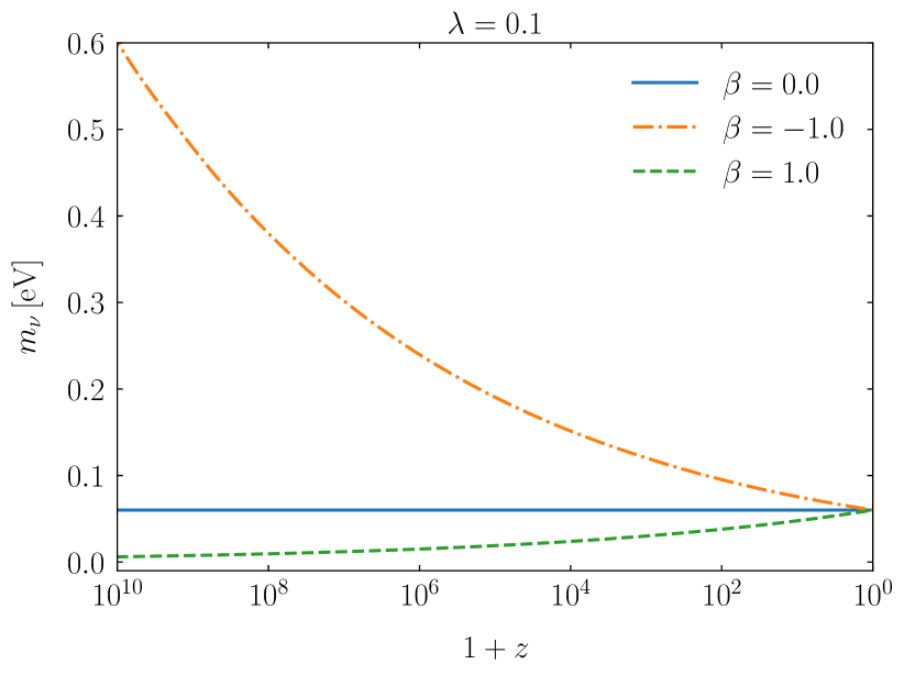
Figure 1: Neutrino mass evolution in growing ($\beta>0$) and shrinking ($\beta<0$) scenarios for ${m_{\nu,0}=0.06\,\mathrm{eV}}$.

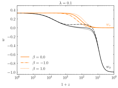
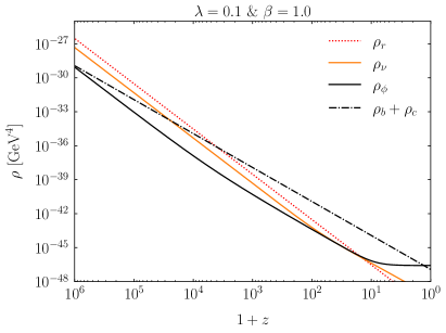
Figure 2: Left panel: Evolution of the equations of state of dark energy ($w_{\phi}$) and of massive neutrinos ($w_{\nu}$) for ${m_{\nu,0}=0.06\,\mathrm{eV}}$ and three illustrative values of $\beta$. Right panel: Evolution of energy densities for ${m_{\nu,0}=0.06\,\mathrm{eV}}$. The radiation energy density ($\rho_{r}$) includes photons and ultrarelatistic neutrinos.

This simple approach is a powerful alternative to the popular CPL parametrization Chevallier and Polarski (2001); Linder (2003), since a large variety of dark energy equation of state evolutions can be captured by just one additional parameter Nunes (2004), thereby limiting the degeneracies in Bayesian inferences. An additional advantage is that the scalar field potential can be reconstructed analytically following Ref. Nunes and Lidsey (2004); da Fonseca et al. (2022b, a); Barros and da Fonseca (2023). This is done by solving the first-order differential equation (7) to find $\rho_{\phi}$ using the constraint equation (1) and noting that ${\dot{\phi}=\lambda H}$ according to Eq. (9). The potential happens to be a sum of exponential terms,

$$V\left(\phi\right)=A\,e^{-\frac{4}{\lambda}\phi}+B\,e^{-\frac{3}{\lambda}\phi}+C\,e^{\left(-\frac{3}{\lambda}+\beta\right)\phi}+D\,e^{-\lambda\phi}\,,$$ (10)

where the mass scales are given by the following analytical expressions,

$$A =\frac{\lambda^{2}}{4-\lambda^{2}}\Omega_{r}H_{0}^{2}\,,$$ (11)

$$B =\frac{3}{2}\frac{\lambda^{2}}{3-\lambda^{2}}\left(\Omega_{b}+\Omega_{c}\right)H_{0}^{2}\,,$$ (12)

$$C =\frac{3}{2}\frac{\lambda^{2}+2\beta\lambda}{3-\lambda^{2}-\beta\lambda}\Omega_{\nu}H_{0}^{2}\,,$$ (13)

$$D =3\left(1-\frac{\lambda^{2}}{6}\right)H_{0}^{2}\left[1+\frac{4}{\lambda^{2}-4}\Omega_{r}\right.$$ (14)

$$\left.+\frac{3}{\lambda^{2}-3}\left(\Omega_{b}+\Omega_{c}\right)+\frac{3}{\lambda^{2}-3+\beta\lambda}\Omega_{\nu}\right]\,,$$

$\Omega_{r}$ includes both photons and ultrarelativist neutrinos. As for the density parameter $\Omega_{\nu}$, it corresponds to those neutrinos that are non-relativistic, and we can write Lesgourgues et al. (2013)

$$\Omega_{\nu}h^{2}=\frac{m_{\nu,0}}{93.14\,\mathrm{eV}}\,.$$ (15)

We specifically modify the CLASS code to evolve the scalar field with the potential and the equation of motion (8). The field parametrization is not implemented as such. Independently of the initial conditions, the potential leads to two successive scaling regimes Barreiro et al. (2000), where the field equation of state, shown in the left panel of Fig. 2, first tracks radiation (${w_{\phi}\sim 1/3}$) and then matter (${w_{\phi}\sim 0}$), before being attracted to the late-time acceleration stage (${w_{\phi}\sim-1}$), always present when ${\lambda^{2}<2}$. At this point, the energy density of the field freezes, mimicking a cosmological constant at late time, as shown in the right panel.

We can see from Fig. 2 that the coupling with neutrinos changes $w_{\phi}$ during the matter-dominated era. For growing masses (${\beta>0}$, dotted line), the field equation of state is smaller compared to the uncoupled case (${\beta=0}$, solid line). On the contrary, $w_{\phi}$ is larger when the energy transfer occurs in the opposite direction, i.e. from neutrinos of shrinking mass (${\beta<0}$, dash-dotted line). Correspondingly, Fig. 3 shows that the non-relativistic neutrinos which receive energy from the scalar field ($\beta>0$) have lower fractional energy density to reach the same present mass than when they give energy ($\beta<0$).

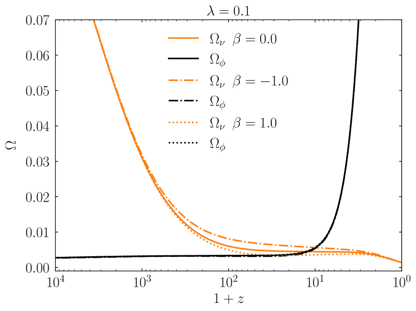
Figure 3: Evolution of the abundances of massive neutrinos and dark energy energy for ${m_{\nu,0}=0.06\,\mathrm{eV}}$

In the early universe, neutrinos are held in equilibrium in the primordial plasma by electroweak interactions with charged leptons tightly coupled to photons by electromagnetic processes. As the temperature of the Universe decreases, the interaction rate drops much faster than the Hubble expansion rate. Around ${1\,\mathrm{MeV}}$, at redshift ${z=1/a-1\sim 10^{10}}$, neutrinos cease to interact with the cosmological plasma and flow freely along geodesics. Unlike other particles, the neutrinos are hot relics that decouple while still ultrarelativistic. Therefore their unperturbed phase-space-distribution function maintains to a good approximation the Fermi-Dirac shape for an ultrarelativistic fermion in thermal equilibrium,

$$f_{0}(q)=\frac{1}{e^{q}+1}\,,$$ (16)

neglecting the chemical potential for neutrinos and antineutrinos (i.e. assuming vanishing lepton asymmetry). ${q=ap/T_{\nu,0}}$ is their normalized comoving momentum, $p$ being the physical momentum, and $T_{\nu,0}$ their current temperature. The unperturbed energy density and pressure of the massive neutrino species are thus given by

$$\rho_{\nu} =\frac{1}{\pi^{2}}\left(\frac{T_{\nu,0}}{a}\right)^{4}\int_{0}^{\infty}f_{0}(q)\,dq\,q^{2}\epsilon\,,$$ (17)

$$p_{\nu} =\frac{1}{3\pi^{2}}\left(\frac{T_{\nu,0}}{a}\right)^{4}\int_{0}^{\infty}f_{0}(q)\,dq\,\frac{q^{4}}{\epsilon}\,,$$ (18)

with

$$\epsilon^{2}=q^{2}+\frac{a^{2}\,m_{\nu}^{2}(\phi)}{T_{\nu,0}^{2}}\,,$$ (19)

where $\epsilon$ is the neutrino comoving energy.

The massive neutrinos in the ultrarelativistic regime, that is up to the non-relativistic transition, behave as standard radiation with their energy density scaling as $a^{-4}$ and ${p_{\nu}=\rho_{\nu}/3}$. In the non-relativistic regime, the coupling term sources the evolution of both the scalar field and the neutrino fluid, the latter behaving as pressureless matter, ${p_{\nu}=0}$, with its energy density scaling as ${a^{-3}\,e^{\beta\phi}}$. Deep in this regime, the direct integration of Eq. (6) gives

$$\rho_{\nu} =3H_{0}^{2}\Omega_{\nu}\,e^{-3N+\beta\phi}\,,$$ (20)

$$=3H_{0}^{2}\Omega_{\nu}\,a^{-3+\beta\lambda}\,,$$ (21)

given that ${\phi\simeq\lambda N\simeq\lambda\ln a}$ in the parametrization.

From the evolution of their equation of state, ${w_{\nu}=p_{\nu}/\rho_{\nu}}$, in the left panel of Fig. 2, we see that neutrinos with shrinking mass (${\beta<0}$, dash-dotted line) become non-relativistic earlier than those with growing mass (${\beta>0}$, dotted line), since the latter are lighter in the past and the transition between the two regimes occurs when the average momentum becomes of the order of the mass, ${\langle p\rangle=3.15\,T_{\nu}=m_{\nu}}$ Gerbino and Lattanzi (2018). The redshift $z_{\mathrm{nr}}$ at which the coupled neutrinos become non-relativistic is given by Gerbino and Lattanzi (2018)

$$1+z_{\mathrm{nr}}\simeq 1900\left(\frac{m_{\nu,0}}{\mathrm{eV}}\right)\,e^{\beta\phi_{\mathrm{nr}}}\,.$$ (22)

According to our choice for the parametrization, ${\phi_{\mathrm{nr}}\simeq-\lambda\ln{(1+z_{\mathrm{nr}})}}$, we get ${e^{\beta\phi_{\mathrm{nr}}}\simeq(1+z_{\mathrm{nr}})^{-\beta\lambda}}$, and thus

$$1+z_{\mathrm{nr}}\simeq\left[1900\left(\frac{m_{\nu,0}}{\mathrm{eV}}\right)\right]^{\frac{1}{1+\beta\lambda}}\,,$$ (23)

where the transition between the two regimes depends on the two extra parameters $\beta$ and $\lambda$ and, as usual, on the current neutrino mass $m_{\nu,0}$.

III Impact of the coupling on perturbations and observables

III.1 Perturbation equations

We apply the theory of linear perturbations Lifshitz (1946) in the synchronous gauge, adopting the usual conventions of Ref. Ma and Bertschinger (1995). In particular, in this section, the scalars $h$ and $\eta$ represent the metric perturbations, and the energy density fluctuation of the cosmological species $i$ is described by the density contrast ${\delta_{i}\equiv\delta\rho_{i}/\bar{\rho_{i}}}$. The overbar denotes the background quantities. The perturbed energy density and pressure of a given species $i$ are ${\delta\rho_{i}\equiv\rho(\bm{x},\tau)-\bar{\rho}_{i}(\tau)}$ and ${\delta p_{i}\equiv p(\bm{x},\tau)-\bar{p}_{i}(\tau)}$ respectively. In this section, the dot denotes derivation with respect to conformal time $d\tau\equiv dt/a$.

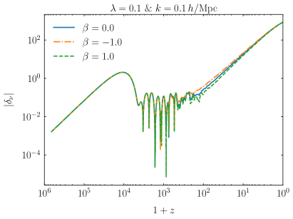
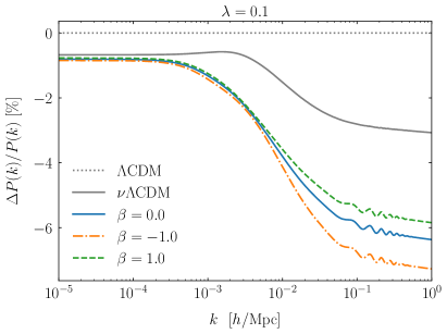
Figure 4: Left panel: Evolution of the massive neutrino perturbations at the scale ${k=0.1\,h/\mathrm{Mpc}}$ for ${\lambda=0.1}$ and ${m_{\nu,0}=0.06\,\mathrm{eV}}$. Right panel: Suppression of the linear matter power spectrum at $z=0$ with respect to the $\Lambda$CDM model.

The perturbed energy density and pressure of the interacting neutrinos have been derived in previous studies (see e.g. Ichiki and Keum (2008); Brookfield et al. (2006); Franca et al. (2009)):

$$\delta\rho_{\nu} =4\pi\left(\frac{T_{\nu,0}}{a}\right)^{4}\int_{0}^{\infty}f_{0}(q)\,dq\,q^{2}\left(\epsilon\Psi+\beta\delta\phi\frac{m^{2}_{\nu}a^{2}}{\epsilon}\right)\,,$$ (24)

$$\delta p_{\nu} =\frac{4\pi}{3}\left(\frac{T_{\nu,0}}{a}\right)^{4}\int_{0}^{\infty}f_{0}(q)\,dq\,\frac{q^{4}}{\epsilon}\left(\Psi-\beta\delta\phi\frac{m^{2}_{\nu}a^{2}}{\epsilon^{2}}\right)\,,$$ (25)

where ${\delta\phi\equiv\phi(\bm{x},t)-\bar{\phi}(t)}$ denotes the fluctuations of the coupled scalar field, and ${\lvert\Psi\rvert\ll 1}$ is the relative perturbation to the neutrino phase-space distribution,

$$\Psi\left(x^{i},q,n_{j},\tau\right)=\frac{f\left(x^{i},q,n_{j},\tau\right)}{f_{0}\left(q\right)}-1\,,$$ (26)

at first order in the perturbations, $f$ being the perturbed distribution function, and ${n^{i}n_{i}=1}$. The dipole equation for the neutrino hierarchy is affected by the interaction, and the corresponding system of infinite equations becomes the following in Fourier space,

$$\dot{\Psi}_{0} =-\frac{qk}{\epsilon}\Psi_{1}+\frac{\dot{h}}{6}\frac{d\ln f_{0}}{d\ln q}\,,$$ (27)

$$\dot{\Psi}_{1} =\frac{qk}{3\epsilon}\left(\Psi_{0}-2\Psi_{2}\right)-\frac{qk}{3\epsilon}\beta\delta\phi\frac{a^{2}m_{\nu}^{2}}{q^{2}}\frac{d\ln f_{0}}{d\ln q}\,,$$ (28)

$$\dot{\Psi}_{2} =\frac{qk}{5\epsilon}\left(2\Psi_{1}-3\Psi_{3}\right)-\left(\frac{\dot{h}}{15}+\frac{2\dot{\eta}}{5}\right)\frac{d\ln f_{0}}{d\ln q}\,,$$ (29)

$$\dot{\Psi}_{\ell\geq 3} =\frac{qk}{\left(2\ell+1\right)\epsilon}\left[\ell\Psi_{\ell-1}-\left(\ell+1\right)\Psi_{\ell+1}\right]\,,$$ (30)

where $\Psi_{\ell}$ is the $\ell$th Legendre component of the series expansion in multipole space of the perturbation $\Psi$. We modified the non cold dark matter part of the CLASS code Lesgourgues and Tram (2011) to evolve the perturbation equations of the MaVaN model.

In the fluid approximation, on sub-Hubble scales, the Boltzmann hierarchy in the momentum grid is cut at ${l_{\mathrm{max}}=2}$ and the continuity equation reads

$$\dot{\delta}_{\nu}= \,3\left(aH+\beta\dot{\phi}\right)\left(w_{\nu}-\frac{\delta p_{\nu}}{\delta\rho_{\nu}}\right)\delta_{\nu}$$

$$-\left(1+w_{\nu}\right)\left(\theta_{\nu}+\frac{\dot{h}}{2}\right)+\beta\left(1-3w_{\nu}\right)\delta\dot{\phi}\,,$$ (31)

where $\theta_{\nu}$ is the neutrino flux divergence. Moreover, the Euler equation is

$$\dot{\theta}_{\nu}= -aH\left(1-3w_{\nu}\right)\theta_{\nu}-\frac{\dot{w}_{\nu}}{1+w_{\nu}}\theta_{\nu}+\frac{\delta p_{\nu}/\delta\rho_{\nu}}{1+w_{\nu}}k^{2}\delta_{\nu}$$

$$+\beta\frac{1-3w_{\nu}}{1+w_{\nu}}k^{2}\delta\phi-\beta\left(1-3w_{\nu}\right)\dot{\phi}\,\theta_{\nu}-k^{2}\sigma_{\nu}\,,$$ (32)

where the neutrino anisotropic stress $\sigma_{\nu}$ Ma and Bertschinger (1995) is not changed by the coupling. We have adjusted the fluid approximation equations of the non cold dark matter in the CLASS code accordingly.

Deep in the non-relativistic regime, when ${w_{\nu}=0}$, the ratio ${q/\epsilon}$ vanishes asymptotically and the pressure perturbations in the neutrino fluid, as well as the shear stress, become negligible with respect to density perturbations. The continuity and Euler equations are analogous to those of the coupled cold dark matter model Amendola (2000); da Fonseca et al. (2022b),

$$\dot{\delta}_{\nu}+\theta_{\nu}+\frac{\dot{h}}{2} =\beta\delta\dot{\phi}\,,$$ (33)

$$\dot{\theta}_{\nu}+aH\theta_{\nu} =\beta\left(k^{2}\delta\phi-\dot{\phi}\theta_{\nu}\right)\,.$$ (34)

For to the coupled scalar field, the equation of motion of the fluctuations is the following,

$$\delta\ddot{\phi}+2aH\delta\dot{\phi}+\left(k^{2}+a^{2}\frac{d^{2}V}{d\phi^{2}}\right)\delta\phi+\frac{1}{2}\dot{h}\dot{\phi}$$

$$=-a^{2}\beta\left(\delta\rho_{\nu}-3\delta p_{\nu}\right)\,.$$ (35)

As in the background, we evolve the field perturbations with the potential through the above equation in our version of the CLASS code.

III.2 Effects on the matter power spectrum

There are three main stages of the evolution of the neutrino density contrast affected by the coupling. During the radiation-dominated era, when the neutrinos are decoupled from the thermal bath but still relativistic, their perturbations grow as radiation. Later, the neutrinos become non-relativistic and cluster in the gravitational potential wells of cold dark matter, which is the dominant cosmological component. However, below their free-streaming scale, they do not cluster like cold dark matter Lesgourgues and Pastor (2006). Neutrino free streaming dampens the neutrino fluctuations up to a critical scale depending on the neutrino mass, and giving the oscillatory pattern seen in the left panel of Fig. 4. The free-streaming wavenumber of Fourrier mode reaches a minimum at the nonrelativistic transition, given by Gerbino and Lattanzi (2018)

$$k_{\mathrm{fs}}\simeq 0.018\,\Omega_{m}^{1/2}\left(\frac{m_{\nu,0}}{\mathrm{eV}}\right)^{1/2}e^{\beta\phi_{\mathrm{nr}}/2}\,h\,\mathrm{Mpc}^{-1}\,,$$ (36)

during matter or dark energy domination. Or equivalently, using Eqs. (22) and (23), we get

$$k_{\mathrm{fs}}\simeq 4.1\cdot 10^{-4}\,\Omega_{m}^{1/2}\left(1900\frac{m_{\nu,0}}{\mathrm{eV}}\right)^{\frac{1}{2(1+\beta\lambda)}}\,h\,\mathrm{Mpc}^{-1}\,,$$ (37)

for our particular scalar field parametrization. Above the free-streaming length, the neutrino fluctuations grow unhindered. For growing neutrino masses (${\beta>0}$, green dashed line) the free-streaming scale in Eq.(37) is larger and the growth of the fluctuations is delayed with respect to shrinking neutrino masses (${\beta<0}$, orange dash-dotted line).

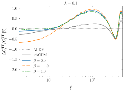
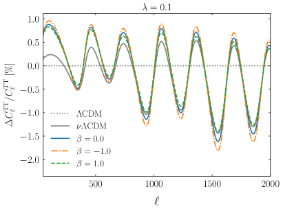
Figure 5: Left panel: Comparison of the power spectra of the CMB anisotropies with respect to $\Lambda$CDM, for ${\lambda=0.1}$ and ${m_{\nu,0}=0.06\,\mathrm{eV}}$, on large and intermediate scales. Right panel: Same as left, on medium and small scales.

Furthermore, the dependence of the neutrino mass on $\beta$ changes the fraction of matter whose fluctuations do not grow like cold dark matter at a given scale. The neutrinos do not contribute to the creation of potential wells below the free streaming scale, and all structure formation is damped because the gravitational wells are not as deep as they would be in the presence of only non-relativistic matter.

The effect of the coupling on the linear matter power spectrum, which is proportional to the variance of the density fluctuations (which tells how large they are at a given scale), can be seen on small scales, at large wavenumbers $k$. The right panel of Fig. 4 shows the residual plot between the MaVaN scenario and the standard $\Lambda$CDM model with massless neutrinos, normalized to the power spectrum of the latter. At scales smaller than the critical scale ($k\gtrsim 10^{-3}$), below which neutrinos do not cluster, the perturbations in the neutrino fluid are completely damped by free streaming and do not contribute to matter perturbations. In this respect, we see with the gray solid line that the ${\nu\Lambda\mathrm{CDM}}$ model suppresses power at these scales compared to the $\Lambda$CDM model with massless neutrinos.

Moreover, the non-negligible fraction of dark energy itself (${\lambda\neq 0}$ and ${\beta=0}$, blue solid line) further reduces the growth of the fluctuations during matter dominance, leading to more power suppression. On the other hand, the matter power spectrum at small scales also depends on how large the neutrino mass was in the past. Growing neutrino masses (${\beta>0}$, green dashed line) reduce the power suppression caused by the scalar field, while shrinking neutrino masses increase the suppression (${\beta<0}$, orange dash-dotted line).

On the contrary, it can be seen that $\beta$ has little influence at large scales ($k\lesssim 10^{-3}$), since the neutrinos cluster independently of their mass.

III.3 Effects on the CMB anisotropies power spectrum

The temperature power spectrum of the unlensed CMB is also affected by the coupling through background and perturbation effects. After their non-relativistic transition, the massive neutrinos modify the evolution of the cosmological background and the redshift of the matter-dark energy equality, with respect to an uncoupled neutrino universe, affecting the Late Time Integrated Sachs Wolf Effect. As shown in the left panel of Fig. 5, at large angular scales (lower multipoles ${\ell\lesssim 20}$) reminiscent of the scale-invariant primordial spectrum of the inflationary perturbations, the additional power produced by the time evolution of the gravitational potentials, as dark energy begins to dominate, decreases with negative couplings (orange dash-dotted line).

On the intermediate scales (${20\lesssim\ell\lesssim 500}$), dominated by the imprints of the acoustic oscillations in the baryon-photon fluid, it is again the effect of the coupling on the evolution of the gravitational potential that affects the first peak. In particular, $\beta$ alters the time required for the gravitational potential to stabilize at a nearly constant value after photon decoupling. Keeping the present value of the Hubble parameter $h$ unchanged, a higher neutrino mass at the time of recombination (${\beta<0}$, orange dash-dotted line) increases the height of the first peak given by the early Integrated Sachs-Wolf effect compared to the $\Lambda$CDM cases. Conversely, the amplitude decreases for a lower neutrino mass at recombination (${\beta>0}$, green dashed line).

The amplitude of the first peak is also affected by the uncoupled scalar field alone (${\beta=0}$, blue solid line). It gives a non-negligible contribution to early dark energy, which reduces the fractional energy density of matter at the time of decoupling da Fonseca et al. (2022a, b). The amplitude increases with the value of $\lambda$.

Moreover, for a given physical density of cold dark matter and baryons, the angle subtended by the sound horizon at recombination, $\theta_{s}$, which determines the spacing between the peaks and in particular the position of the first one, is larger for growing neutrino masses ($\beta>0$). The corresponding shift of the position of the CMB peaks towards larger scales can be compensated by the Hubble constant. Indeed, decreasing $H_{0}$ increases the comoving angular diameter distance from the CMB surface and shifts the peaks towards smaller scales.

At small scales (${\ell\gtrsim 500}$), in the right panel of Fig. 5, of the order of the photon mean free path at the time of recombination, a positive coupling (orange dash-dotted line) has the opposite effect of $\lambda$ (${\beta=0}$, blue solid curve) on the exponential damping of the CMB peak structure.

III.4 Effects on the CMB lensing potential

Because the free-streaming neutrinos erase the density perturbations, they affect the CMB light which is distorted by the gravitational lensing caused by the intervening matter distribution between us and the last scattering surface Lesgourgues et al. (2006). The neutrinos reduce the CMB lensing potential, which is a measure of the integral of the gravitational potentials along the line of sight between the recombination time and the present time. The effect of the weak lensing is to smooth the power spectrum of the CMB temperature anisotropies on small scales. Note in Fig. 6 that since the effect is proportional to the energy density of the neutrinos, it can constrain their mass, whose cosmological evolution is controlled by the two parameters $\lambda$ and $\beta$. For example, if the neutrino mass had been too high in the recent past, we would have had less lensing than we observe. The suppression already caused by the scalar field (${\beta=0}$, blue solid curve) is either enhanced by shrinking neutrino masses ($\beta<0$, orange dash-dotted line) or compensated by growing neutrino masses ($\beta>0$, green dashed line).

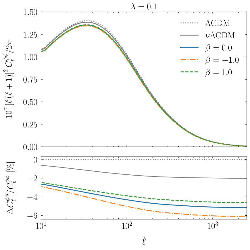
Figure 6: Upper panel: Power spectra of the CMB lensing potential of the $\Lambda$CDM and $\nu\Lambda\mathrm{CDM}$ models, and the coupled scenario with $\lambda=0.1$ and $\sum m_{\nu}=0.06\,\mathrm{eV}$. Lower panel: Percentage deviation between models with respect to $\Lambda$CDM.

It is worth noting that, in contrast to the model-independent parametrization for the neutrino mass variation studied in Ref. Franca et al. (2009), we do not find instabilities on large scales in our model Bjaelde et al. (2008), which would be triggered by large coupling values causing the neutrino perturbations to grow rapidly on the largest scales observable.

IV Parameter estimation

IV.1 Methodology

We choose to test the model with the 2018 Planck satellite Planck Collaboration et al. (2011) temperature and polarization measurements of the CMB at the time of last scattering, combined with the CMB lensing potential as a probe of the distribution and evolution of large-scale structure in the late Universe. We also add Baryon Acoustic Oscillation (BAO) distance and expansion rate measurements in galaxy clusters ”Eisenstein and others” (2005); Cole et al. (2005) covering different redshift ranges. They constrain the model at the background level Percival et al. (2007) to help break the geometric degeneracy between $H_{0}$ and $\sum m_{\nu}$.

With respect to the Planck observations, the Bayesian inference is performed using the CMB lensing potential power spectrum Aghanim et al. (2020b), as well as the cross-correlation likelihoods of the temperature and polarization anisotropies, $TT$, $EE$, and $TE$, respectively Aghanim et al. (2020c). We reduce the dimensional parameter space by using the lite version of the Planck likelihood on the smaller angular scales, which marginalizes the foreground and instrumental effects, leaving the absolute calibration $A_{\mathrm{planck}}$ as the only nuisance parameter. As for the background probe, we use a compilation of measurements that have detected the BAO peak at different angular separations with galaxy samples at different redshifts. The three data points are from the Sloan Digital Sky Survey (SDSS) DR7 Main Galaxy Sample Ross et al. (2015), the SDSS DR9 release Ahn et al. (2012), and the 6dF Galaxy Survey Beutler et al. (2011) respectively. We will refer to our data set as Plk18+BAO in the rest of the document.

Our dedicated version of the CLASS code is used to compute the observables confronting the actual data, on the basis of the sampled parameters $\{\lambda,\beta,\sum m_{\nu}\}$ along with the six standard minimal baseline parameters $\{\Omega_{b}h^{2},\Omega_{c}h^{2},\theta_{s},A_{s},n_{s},\tau_{\mathrm{reio}}\}$. We use $\theta_{s}$ instead of $h$ because it is the quantity measured in the CMB observations. $A_{s}$ is the power of the primordial curvature perturbations normalised at the pivot scale ${k=0.05\,\mathrm{Mpc}^{-1}}$, and $n_{s}$ is the power-law index of the scalar spectrum. $\tau_{\mathrm{reio}}$ is the optical depth to reionization, which gives the fraction of photons re-scattered by the new population of free electrons from the ionization of neutral hydrogen produced by the light of the first stars. The settings in CLASS are such that the effective number of neutrino families is $N_{\mathrm{eff}}=3.044$ Froustey et al. (2020); Bennett et al. (2021), and the neutrino fractional energy density satisfies Eq. (17).

The likelihoods are minimized using the Monte Carlo code of the MontePython parameter estimation package Audren et al. (2013); Brinckmann and Lesgourgues (2019), which samples the parameter space and the posterior probability distributions using a Metropolis-Hastings algorithm with the flat priors specified in Table 1. The size of the prior intervals is sufficient for the corresponding posteriors to fall exponentially within them, except for the parameter $\beta$ as we will discuss later.

Table 1: Flat priors for the sampled model and cosmological parameters.

Parameter	Prior
$\lambda$	$[0,1.4]$
$\beta$	$[0,100]$
$\sum m_{\nu}$	$[0,2]$
$\Omega_{b}h^{2}$	$[0.005,0.1]$
$\Omega_{c}h^{2}$	$[0.01,0.99]$
$100\theta{}_{s}$	$[1,2]$
$\ln 10^{10}A_{s}$	$[2.7,4]$
$n_{s}$	$[0.5,1.5]$
$\tau{}_{\mathrm{reio}}$	$[0.04,0.8]$

We use the Getdist analyzer Lewis (2019) to obtain the constraints from the Markov chains, and plot the confidence contours and the marginalized posterior distributions. In addition to the sampled parameters, we also infer constraints on derived late-Universe parameters : $H_{0}$, $\Omega_{m}$, $\sigma_{8}$ (which measures the amplitude of matter fluctuation on ${8\,h^{-1}\mathrm{Mpc}}$ comoving scale), and the degeneracy parameter ${S_{8}\equiv\sigma_{8}\sqrt{\Omega_{m}/0.3}}$.

IV.2 Main results

The results of the likelihood analysis are summarized in Table 2, which lists the constraints on the cosmological parameters obtained with the Plk18+BAO data set for both the uncoupled ($\beta=0$) scalar field model and the coupled MaVaN model. They lead to several remarkable conclusions.

Table 2: Cosmological constraints (95% limits for $\sum m_{\nu}$, mean and $68\%$ limits for the others) for the uncoupled (${\beta=0}$) and MaVaN ($\beta$ free) models.

Parameter	$\beta=0$	$\hskip 28.45274pt\beta$ free
$\lambda$	$<0.0472$	$\hskip 28.45274pt0.059^{+0.029}_{-0.037}$
$\sum m_{\nu}$	$<0.127$	$\hskip 28.45274pt<0.724$
$\Omega_{b}h^{2}$	$0.02241\pm 0.00014$	$\hskip 28.45274pt0.02242\pm 0.00014$
$\Omega_{c}h^{2}$	$0.1199\pm 0.0011$	$\hskip 28.45274pt0.1200\pm 0.0011$
$100\theta{}_{s}$	$1.04186\pm 0.00030$	$\hskip 28.45274pt1.04179\pm 0.00031$
$\ln 10^{10}A_{s}$	$3.050^{+0.014}_{-0.016}$	$\hskip 28.45274pt3.049^{+0.014}_{-0.016}$
$n_{s}$	$0.9667\pm 0.0039$	$\hskip 28.45274pt0.9669\pm 0.0039$
$\tau{}_{\mathrm{reio}}$	$0.0568^{+0.0068}_{-0.0082}$	$\hskip 28.45274pt0.0564^{+0.0068}_{-0.0080}$
$H_{0}$	$67.59^{+0.69}_{-0.57}$	$\hskip 28.45274pt67.61^{+0.65}_{-0.56}$
$\Omega_{m}$	$0.3127^{+0.0074}_{-0.0091}$	$\hskip 28.45274pt0.3176^{+0.0084}_{-0.012}$
$\sigma_{8}$	$0.813^{+0.012}_{-0.0079}$	$\hskip 28.45274pt0.804^{+0.019}_{-0.010}$
$S_{8}$	$0.830\pm 0.012$	$\hskip 28.45274pt0.827\pm 0.015$
$A_{\mathrm{planck}}$	$1.0008\pm 0.0025$	$\hskip 28.45274pt1.0007\pm 0.0025$

First, in the uncoupled scalar field model (${\beta=0}$), the dynamical dark energy component is constrained to be close to a cosmological constant, ${\lambda<0.05}$ (68%CL) and ${\lambda<0.09}$ (95%CL), with a clear preference for a vanishing scalar field parameter. This is the result of the extreme constraining power of the CMB data on the fraction of early dark energy at the last scattering surface Gómez-Valent et al. (2021, 2022). In our scalar field parametrization, the fraction of dark energy (during the scaling regime with matter) is given by $\Omega_{\phi}=\lambda^{2}/3$ da Fonseca et al. (2022b), which implies $\Omega_{\phi}<0.27\%$ ($95\%\mathrm{CL}$) at recombination. It is therefore not surprising that the corresponding upper limit ${\sum m_{\nu}<0.127\,\mathrm{eV}}$ (95%CL) that we find is in agreement with recent literature findings for the concordance model based on comparable data sets. For example, including the latest release of BAO eBOSS data in combination with Planck temperature, polarization, and lensing measurements gives an upper limit of ${0.129\,\mathrm{eV}}$ (95%CL) for the uncoupled ${\nu\Lambda\mathrm{CDM}}$ model Alam et al. (2021).

Second, we find that the parameter $\beta$ of the MaVaN model, with our choice of scalar field parametrization, is not constrained by the cosmological observations Plk18+BAO, as shown in Fig. 7 (and Appendix A for additional contour and probability distribution plots). However, the interaction does relax the upper bound on the current neutrino mass sum, raising it significantly by almost a factor of six to ${\sum m_{\nu}<0.724\,\mathrm{eV}}$ (95%CL). Positive couplings allow for the possibility of heavier neutrinos today. Despite their current higher mass, the influence of neutrinos with growing mass on the cosmological expansion and perturbations over time is tempered by the fact that they were lighter in the past and gradually gained energy from the scalar field. Moreover, for the MaVaN model, the data favor a non-vanishing scalar field parameter, ${\lambda=0.059^{+0.029}_{-0.037}}$ (68%CL), at the one-sigma level.

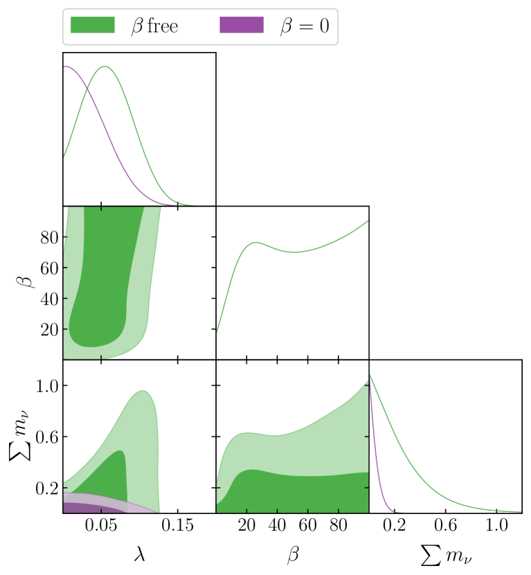
Figure 7: Constraints obtained with the Plk18+BAO data set on the additional parameters. Probability distributions and 2D marginalised contours (68% and 95% CL).

Third, with respect to the standard cosmological parameters, the main differences between the MaVaN model and the uncoupled one are in the matter fluctuation amplitude, $\sigma_{8}$, and the matter density parameter, $\Omega_{m}$. Including the coupling parameter degrades the error bars while virtually preserving the central values, which are consistent with the best fit of the base-$\Lambda$CDM cosmology predicted by the 2018 Planck data Aghanim et al. (2020a). This is particularly the case for the derived parameter $\sigma_{8}$, whose precision decreases by about $50\%$, from $0.813^{+0.012}_{-0.0079}$ to $0.804^{+0.019}_{-0.010}$ (68%CL), mainly towards lower values, which could tend to reduce the tension with late cosmological probes Amon et al. (2022); Abbott et al. (2023); Secco et al. (2022). However, the confidence interval of $\Omega_{m}$ increases by $22\%$ in the opposite direction due to the added fractional energy density of heavier neutrinos, from $0.3126^{+0.0074}_{-0.0090}$ to $0.3176^{+0.0084}_{-0.012}$ (68%CL). As shown in Appendix A, the posterior distribution for the degeneracy parameter $S_{8}$ is only slightly changed by the coupling parameter. As for $H_{0}$, its posterior distribution is hardly modified by the interaction, confirming the inability of the model to resolve the Hubble tension. The fractional dark energy in the early times is far less than the minimum $10\%$ required by neutrino-assisted early dark energy models to improve the $H_{0}$ tension Poulin et al. (2019); de Souza and Rosenfeld (2023).

Finally, to assess the influence of the coupling on the posterior $\sum m_{\nu}$, we repeat the statistical analysis fixing different values for $\beta$. The results are summarized in Table 3 and Fig. 8. For a mass-shrinking neutrino scenario (${\beta=-1}$), the constraint on today’s mass is tighter (${\sum m_{\nu}<0.102\,\mathrm{eV}}$) than without interaction. Large masses in the past are disfavored by the cosmological data. On the contrary, the limit on today’s neutrino masses relaxes as the value of the positive coupling increases. The highest limit is for $\beta=100$, i.e. for the edge of the prior, with $\sum m_{\nu}<1.130\,\mathrm{eV}$ already exceeding the limit obtained by local experiments Aker et al. (2019). Moreover, there seems to be a plateau around $\beta=20$ where the present mass stabilizes in the ($\beta,\sum m_{\nu}$) plane of the parameter space (see also Fig. 7). In addition, as seen earlier, the energy transferred by the scalar field causes the model to deviate slightly from a constant dark energy component. Dark energy moves away from a cosmological constant as the strength of the coupling increases. However, the value of the scalar field parameter is tightly constrained by the CMB data, which does not allow $\lambda$ to be too large, while it could theoretically be as large as $\sqrt{2}$.

Table 3: Constraints on present neutrino mass in eV and on the dark energy parameter $\lambda$, for different coupling values $\beta$.

$\beta$	$\sum m_{\nu}\,(95\%\,\mathrm{CL})$	$\lambda\,(68\%\,\mathrm{CL})$
-1	$<0.102$	$<0.0497$
0	$<0.127$	$<0.0472$
1	$<0.147$	$<0.0493$
5	$<0.355$	$0.046^{+0.016}_{-0.043}$
10	$<0.580$	$0.050^{+0.022}_{-0.038}$
20	$<0.542$	$0.052^{+0.024}_{-0.038}$
30	$<0.513$	$0.053^{+0.025}_{-0.039}$
50	$<0.598$	$0.059^{+0.028}_{-0.037}$
75	$<0.822$	$0.064^{+0.031}_{-0.035}$
100	$<1.130$	$0.067\pm 0.030$
free	$<0.724$	$0.059^{+0.029}_{-0.037}$

We note in Fig. 8 that the $\sum m_{\nu}$ positive and negative correlations with $\Omega_{m}$ and $\sigma_{8}$ respectively are preserved by the coupling. The errors on $S_{8}$ are degraded to lower values as the strength of the interaction increases. It is also worth noting that the degeneracy in the ($\sum m_{\nu},H_{0}$) plane, along which the position of the first CMB peak is held unchanged, decreases significantly with increasing value of the parameter $\beta$, weakening the otherwise strong correlation between the neutrino mass and the Hubble constant. This is probably due to the fact that the posterior for $\lambda$ becomes larger with increasing $\beta$. The corresponding non-negligible fraction of dark energy at the time of recombination reduces the sound horizon at decoupling, thus competing with the geometric degeneracy $\sum m_{\nu}-H_{0}$.

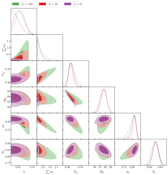
Figure 8: Constraints obtained for fixed coupling parameters. Probability distributions and 2D marginalized contours (68% and 95% CL).

V Discussion

In this study, we investigated a model of mass-varying neutrinos in which the mass depends on the value of a scalar field representing the dark energy component. The originality of our work lies in the choice of the quintessence parametrization, which limits the number of free parameters with respect to other approaches such as the CPL parametrization or arbitrary choices of scalar field potentials. While the parametrization is purely phenomenological, it leads to the analytical reconstruction of the potential as a sum of exponential terms, which conveniently endows dark energy with scaling properties. We have introduced two additional free parameters with respect to $\Lambda$CDM, $\beta$ for the coupling strength between the two sectors in Eq. (2) and $\lambda$ for the linear evolution of the field in Eq. (9).

We confirmed the conjecture that a growing neutrino mass scenario relaxes the upper bound on the current neutrino mass derived in the framework of the baseline $\nu\Lambda$CDM model. Our goal was to complement previous work, such as the study in Ref. Brookfield et al. (2006). In the latter, one of the models considered by the authors was a mass-varying neutrino theory with a constant coupling to the scalar field and a quintessential potential in the form of an exponential. In contrast to our case, their model shows no tracking behavior and allows only shrinking mass scenarios. They also found that astronomical observations do not provide strong constraints on the coupling parameter. To constrain the coupling, they fixed the neutrino mass to values higher than ${0.1\,\mathrm{eV}}$, assuming that such a significant mass could be independently confirmed. Alternately, in our likelihood analysis, we set different values of the coupling to constrain the current neutrino mass.

Following the analysis of the model at background level, we evaluated the sensitivity of several observables (matter and CMB power spectra, and CMB lensing potential) to the coupling, using a version of the Boltzmann code CLASS that we adapted to the considered model. We found that growing neutrino masses lead to less matter power suppression than predicted by the presence of a non-interacting scalar field. The coupling also affects the shape of the CMB power spectrum at different scales, in particular through the integrated Sachs-Wolf effect, in parallel with the effect of the scalar field parameter itself. The CMB lensing potential is sensitive to the interaction. Growing neutrino masses can compensate for the reduction in lensing potential caused by the quintessence fluid. It is therefore theoretically possible to obtain constraints on a putative interaction between the neutrino sector and a dynamical dark energy component.

We performed Bayesian inferences to estimate the parameters of the model using observations of CMB temperature and polarization anisotropies and lensing from the Planck satellite, together with BAO measurements. This data set allows us to combine cosmological probes covering the early universe at the time of the last scattering, the formation of large-scale structures in the late universe, and the cosmic expansion history. The Markov chains were generated by the MontePython package using a Metropolis-Hastings algorithm to explore the parameter space, which contains nine free parameters, $\{\lambda,\beta,\sum m_{\nu},\Omega_{b}h^{2},\Omega_{c}h^{2},\theta_{s},A_{s},n_{s},\tau_{\mathrm{reio}}\}$, plus one nuisance parameter $A_{\mathrm{planck}}$. We also derived constraints on four late universe parameters: $H_{0}$, $\sigma_{8}$, $\Omega_{m}$ and $S_{8}$.

The main conclusion is that the model relaxes the upper bound on the neutrino mass, from ${\sum m_{\nu}<0.13\,\mathrm{eV}}$ in $\nu\Lambda$CDM to ${\sum m_{\nu}<0.72\,\mathrm{eV}}$ in our model (95%CL). The dynamical property of dark energy is enhanced because the scalar field looses energy to the neutrino, whose mass grows with time. With a non-vanishing scalar field parameter, ${\lambda=0.059^{+0.028}_{-0.036}}$ (68%CL), the data disfavors a static field. This is in contrast with previous work where CMB data constraining a scalar field interacting with dark matter model favors $\Lambda$CDM da Fonseca et al. (2022b). The coupling $\beta$ is, however, poorly constrained by the observations of the selected data set. As for the cosmological parameters of the standard model, it is mostly the confidence intervals for $\sigma_{8}$ and $\Omega_{m}$ that are broadened by the interaction, but in a way that weakly affects the posterior distribution of the degeneracy parameter $S_{8}$. The posterior distribution of $H_{0}$ is also almost unchanged, as expected. The scalar field parameter is extremely constrained and the fraction of dark energy at the last scattering is too small to make any impact in resolving the Hubble tension.

In what respects future work, it would be worthwhile to complement the CMB constraints that the Planck data place on the parameters of our model with precise measurements of the anisotropies at larger multipoles ($l\gtrsim 3000$). These small angular scales measured with sufficient accuracy can reveal coupling signatures, especially when the strength of the interaction is small Brax et al. (2023a). For example, an indication of non-vanishing coupling between neutrinos and dark matter at the one-sigma level has been found using the Atacama Cosmology Telescope’s (ACT) high-multipole observations of CMB temperature and polarization anisotropies Brax et al. (2023b). In addition, alternative CMB data on the lensing power spectrum could also be used to further constrain the neutrino – scalar field interaction scenario affecting structure growth Qu et al. (2023). As for the late-time universe probes of large-scale structure, it would be adequate to use the KiDS weak lensing observations Hildebrandt et al. (2017) to test the MaVaN model, like in the coupled dark matter case da Fonseca et al. (2022b).

Appendix A Parameter constraints for the MaVaN and the uncoupled scalar field models

In the appendix we show the triangular plots of the analysis made with the Plk18+BAO data for the MaVaN model ($\beta$ free) and the uncoupled case ($\beta=0$), i.e. no interaction between the quintessence component and the neutrino fluid.

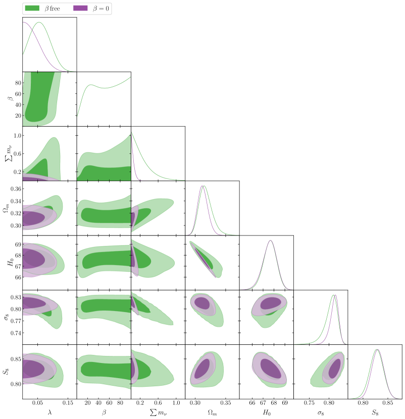
Figure 9: Probability distributions and 2D marginalized contours (68% and 95% CL) obtained with the Plk18+BAO data set.

References

- Lesgourgues and Pastor (2006) J. Lesgourgues and S. Pastor, Phys. Rept. 429, 307 (2006), arXiv:astro-ph/0603494 .
- Gerbino and Lattanzi (2018) M. Gerbino and M. Lattanzi, Frontiers in Physics 5 (2018), 10.3389/fphy.2017.00070.
- Fukuda et al. (1998) Y. Fukuda et al. (Super-Kamiokande), Phys. Rev. Lett. 81, 1562 (1998), arXiv:hep-ex/9807003 .
- Abe et al. (2014) K. Abe et al. (T2K), Phys. Rev. Lett. 112, 061802 (2014), arXiv:1311.4750 [hep-ex] .
- Esteban et al. (2019) I. Esteban, M. C. Gonzalez-Garcia, A. Hernandez-Cabezudo, M. Maltoni, and T. Schwetz, JHEP 01, 106 (2019), arXiv:1811.05487 [hep-ph] .
- Roy Choudhury and Hannestad (2020) S. Roy Choudhury and S. Hannestad, JCAP 07, 037 (2020), arXiv:1907.12598 [astro-ph.CO] .
- Aker et al. (2019) M. Aker et al. (KATRIN), Phys. Rev. Lett. 123, 221802 (2019), arXiv:1909.06048 [hep-ex] .
- Gershtein and Zel’dovich (1966) S. S. Gershtein and Y. B. Zel’dovich, ZhETF Pisma Redaktsiiu 4, 174 (1966).
- Aghanim et al. (2020a) N. Aghanim et al. (Planck), A&A 641, A6 (2020a), [Erratum: Astron.Astrophys. 652, C4 (2021)], arXiv:1807.06209 [astro-ph.CO] .
- Workman et al. (2022) R. L. Workman et al. (Particle Data Group), PTEP 2022, 083C01 (2022).
- Riess et al. (1998) A. G. Riess et al. (Supernova Search Team), Astron. J. 116, 1009 (1998), arXiv:astro-ph/9805201 .
- Perlmutter et al. (1999) S. Perlmutter et al. (Supernova Cosmology Project), Astrophys. J. 517, 565 (1999), arXiv:astro-ph/9812133 .
- Gu et al. (2003) P. Gu, X. Wang, and X. Zhang, Phys. Rev. D 68, 087301 (2003), arXiv:hep-ph/0307148 .
- Fardon et al. (2004) R. Fardon, A. E. Nelson, and N. Weiner, JCAP 10, 005 (2004), arXiv:astro-ph/0309800 .
- Peccei (2005) R. D. Peccei, Phys. Rev. D 71, 023527 (2005), arXiv:hep-ph/0411137 .
- Brookfield et al. (2006) A. W. Brookfield, C. van de Bruck, D. F. Mota, and D. Tocchini-Valentini, Phys. Rev. D 73, 083515 (2006), [Erratum: Phys.Rev.D 76, 049901 (2007)], arXiv:astro-ph/0512367 .
- Wetterich (2007) C. Wetterich, Phys. Lett. B 655, 201 (2007), arXiv:0706.4427 [hep-ph] .
- Amendola et al. (2008) L. Amendola, M. Baldi, and C. Wetterich, Phys. Rev. D 78, 023015 (2008), arXiv:0706.3064 [astro-ph] .
- Ichiki and Keum (2008) K. Ichiki and Y.-Y. Keum, JCAP 06, 005 (2008), arXiv:0705.2134 [astro-ph] .
- Franca et al. (2009) U. Franca, M. Lattanzi, J. Lesgourgues, and S. Pastor, Phys. Rev. D 80, 083506 (2009), arXiv:0908.0534 [astro-ph.CO] .
- Geng et al. (2016) C.-Q. Geng, C.-C. Lee, R. Myrzakulov, M. Sami, and E. N. Saridakis, JCAP 01, 049 (2016), arXiv:1504.08141 [astro-ph.CO] .
- Nunes and Lidsey (2004) N. J. Nunes and J. E. Lidsey, Phys. Rev. D 69, 123511 (2004), arXiv:astro-ph/0310882 .
- Peebles and Ratra (1988) P. J. E. Peebles and B. Ratra, apjl 325, L17 (1988).
- da Fonseca et al. (2022a) V. da Fonseca, T. Barreiro, N. J. Nunes, S. Cristiani, et al., Astronomy & Astrophysics (2022a), 10.1051/0004-6361/202243795.
- Barros and da Fonseca (2023) B. J. Barros and V. da Fonseca, JCAP 06, 048 (2023), arXiv:2209.12189 [astro-ph.CO] .
- da Fonseca et al. (2022b) V. da Fonseca, T. Barreiro, and N. J. Nunes, Phys. Dark Univ. 35, 100940 (2022b), arXiv:2104.14889 [astro-ph.CO] .
- Mota et al. (2008) D. F. Mota, V. Pettorino, G. Robbers, and C. Wetterich, Phys. Lett. B 663, 160 (2008), arXiv:0802.1515 [astro-ph] .
- Nunes et al. (2011) N. J. Nunes, L. Schrempp, and C. Wetterich, Phys. Rev. D 83, 083523 (2011), arXiv:1102.1664 [astro-ph.CO] .
- Sakstein and Trodden (2020) J. Sakstein and M. Trodden, Phys. Rev. Lett. 124, 161301 (2020), arXiv:1911.11760 [astro-ph.CO] .
- Carrillo González et al. (2023) M. Carrillo González, Q. Liang, J. Sakstein, and M. Trodden, (2023), arXiv:2302.09091 [astro-ph.CO] .
- Riess et al. (2019) A. G. Riess, S. Casertano, W. Yuan, L. M. Macri, and D. Scolnic, Astrophys. J. 876, 85 (2019), arXiv:1903.07603 [astro-ph.CO] .
- Wong et al. (2020) K. C. Wong et al., Mon. Not. Roy. Astron. Soc. 498, 1420 (2020), arXiv:1907.04869 [astro-ph.CO] .
- Riess et al. (2021) A. G. Riess, S. Casertano, W. Yuan, J. B. Bowers, L. Macri, J. C. Zinn, and D. Scolnic, Astrophys. J. Lett. 908, L6 (2021), arXiv:2012.08534 [astro-ph.CO] .
- Lesgourgues (2011) J. Lesgourgues, “The cosmic linear anisotropy solving system (class) i: Overview,” (2011), arXiv:1104.2932 [astro-ph.IM] .
- Blas et al. (2011) D. Blas, J. Lesgourgues, and T. Tram, JCAP 2011, 034–034 (2011).
- Slosar (2006) A. c. v. Slosar, Phys. Rev. D 73, 123501 (2006).
- Font-Ribera et al. (2014) A. Font-Ribera, P. McDonald, N. Mostek, B. A. Reid, H.-J. Seo, and A. Slosar, JCAP 05, 023 (2014), arXiv:1308.4164 [astro-ph.CO] .
- Di Valentino et al. (2018) E. Di Valentino et al. (CORE), JCAP 04, 017 (2018), arXiv:1612.00021 [astro-ph.CO] .
- Damour et al. (1990) T. Damour, G. W. Gibbons, and C. Gundlach, Phys. Rev. Lett. 64, 123 (1990).
- Chevallier and Polarski (2001) M. Chevallier and D. Polarski, International Journal of Modern Physics D 10, 213 (2001).
- Linder (2003) E. Linder, Physical review letters 90, 091301 (2003).
- Nunes (2004) N. J. Nunes, AIP Conf. Proc. 736, 135 (2004).
- Lesgourgues et al. (2013) J. Lesgourgues, G. Mangano, G. Miele, and S. Pastor, Neutrino Cosmology (Cambridge University Press, 2013).
- Barreiro et al. (2000) T. Barreiro, E. J. Copeland, and N. J. Nunes, Phys. Rev. D 61, 127301 (2000).
- Lifshitz (1946) E. Lifshitz, J. Phys. (USSR) 10, 116 (1946).
- Ma and Bertschinger (1995) C.-P. Ma and E. Bertschinger, Astrophys. J. 455, 7 (1995), arXiv:astro-ph/9506072 .
- Lesgourgues and Tram (2011) J. Lesgourgues and T. Tram, Journal of Cosmology and Astroparticle Physics 2011, 032 (2011).
- Amendola (2000) L. Amendola, Mon. Not. Roy. Astron. Soc. 312, 521 (2000), arXiv:astro-ph/9906073 .
- Lesgourgues et al. (2006) J. Lesgourgues, L. Perotto, S. Pastor, and M. Piat, Phys. Rev. D 73, 045021 (2006), arXiv:astro-ph/0511735 .
- Bjaelde et al. (2008) O. E. Bjaelde, A. W. Brookfield, C. van de Bruck, S. Hannestad, D. F. Mota, L. Schrempp, and D. Tocchini-Valentini, JCAP 01, 026 (2008), arXiv:0705.2018 [astro-ph] .
- Planck Collaboration et al. (2011) Planck Collaboration, Ade, P. A. R., Aghanim, N., et al., A&A 536, A1 (2011).
- ”Eisenstein and others” (2005) D. J. ”Eisenstein and others” (SDSS), Astrophys. J. 633, 560 (2005), arXiv:astro-ph/0501171 .
- Cole et al. (2005) S. Cole et al. (2dFGRS), Mon. Not. Roy. Astron. Soc. 362, 505 (2005), arXiv:astro-ph/0501174 .
- Percival et al. (2007) W. J. Percival, S. Cole, D. J. Eisenstein, R. C. Nichol, J. A. Peacock, A. C. Pope, and A. S. Szalay, Mon. Not. Roy. Astron. Soc. 381, 1053 (2007), arXiv:0705.3323 [astro-ph] .
- Aghanim et al. (2020b) N. Aghanim et al. (Planck), Astron. Astrophys. 641, A8 (2020b), arXiv:1807.06210 [astro-ph.CO] .
- Aghanim et al. (2020c) N. Aghanim et al. (Planck), Astron. Astrophys. 641, A5 (2020c), arXiv:1907.12875 [astro-ph.CO] .
- Ross et al. (2015) A. J. Ross, L. Samushia, C. Howlett, W. J. Percival, A. Burden, and M. Manera, Mon. Not. Roy. Astron. Soc. 449, 835 (2015), arXiv:1409.3242 [astro-ph.CO] .
- Ahn et al. (2012) C. P. Ahn et al., The Astrophysical Journal Supplement Series 203, 21 (2012).
- Beutler et al. (2011) F. Beutler, C. Blake, M. Colless, D. H. Jones, L. Staveley-Smith, L. Campbell, Q. Parker, W. Saunders, and F. Watson, Monthly Notices of the Royal Astronomical Society 416, 3017 (2011).
- Froustey et al. (2020) J. Froustey, C. Pitrou, and M. C. Volpe, JCAP 12, 015 (2020), arXiv:2008.01074 [hep-ph] .
- Bennett et al. (2021) J. J. Bennett, G. Buldgen, P. F. De Salas, M. Drewes, S. Gariazzo, S. Pastor, and Y. Y. Y. Wong, JCAP 04, 073 (2021), arXiv:2012.02726 [hep-ph] .
- Audren et al. (2013) B. Audren, J. Lesgourgues, K. Benabed, and S. Prunet, JCAP 2013, 001 (2013), arXiv:1210.7183 [astro-ph.CO] .
- Brinckmann and Lesgourgues (2019) T. Brinckmann and J. Lesgourgues, Physics of the Dark Universe 24, 100260 (2019).
- Lewis (2019) A. Lewis, “GetDist: Monte Carlo sample analyzer,” Astrophysics Source Code Library, record ascl:1910.018 (2019), arXiv:1910.13970 [astro-ph.IM] .
- Gómez-Valent et al. (2021) A. Gómez-Valent, Z. Zheng, L. Amendola, V. Pettorino, and C. Wetterich, Phys. Rev. D 104, 083536 (2021), arXiv:2107.11065 [astro-ph.CO] .
- Gómez-Valent et al. (2022) A. Gómez-Valent, Z. Zheng, L. Amendola, C. Wetterich, and V. Pettorino, Phys. Rev. D 106, 103522 (2022), arXiv:2207.14487 [astro-ph.CO] .
- Alam et al. (2021) S. Alam et al. (eBOSS), Phys. Rev. D 103, 083533 (2021), arXiv:2007.08991 [astro-ph.CO] .
- Amon et al. (2022) A. Amon et al. (DES), Phys. Rev. D 105, 023514 (2022), arXiv:2105.13543 [astro-ph.CO] .
- Abbott et al. (2023) T. M. C. Abbott et al. (Kilo-Degree Survey, DES), (2023), arXiv:2305.17173 [astro-ph.CO] .
- Secco et al. (2022) L. F. Secco et al. (DES), Phys. Rev. D 105, 023515 (2022), arXiv:2105.13544 [astro-ph.CO] .
- Poulin et al. (2019) V. Poulin, T. L. Smith, T. Karwal, and M. Kamionkowski, Phys. Rev. Lett. 122, 221301 (2019), arXiv:1811.04083 [astro-ph.CO] .
- de Souza and Rosenfeld (2023) D. H. F. de Souza and R. Rosenfeld, (2023), arXiv:2302.04644 [astro-ph.CO] .
- Brax et al. (2023a) P. Brax, C. van de Bruck, E. Di Valentino, W. Giarè, and S. Trojanowski, (2023a), arXiv:2303.16895 [astro-ph.CO] .
- Brax et al. (2023b) P. Brax, C. van de Bruck, E. Di Valentino, W. Giarè, and S. Trojanowski, Phys. Dark Univ. 42, 101321 (2023b), arXiv:2305.01383 [astro-ph.CO] .
- Qu et al. (2023) F. J. Qu et al. (ACT), (2023), arXiv:2304.05202 [astro-ph.CO] .
- Hildebrandt et al. (2017) H. Hildebrandt et al., Mon. Not. Roy. Astron. Soc. 465, 1454 (2017), arXiv:1606.05338 [astro-ph.CO] .