On the Generalization Properties of Diffusion Models
Abstract
Diffusion models are a class of generative models that serve to establish a stochastic transport map between an empirically observed, yet unknown, target distribution and a known prior. Despite their remarkable success in real-world applications, a theoretical understanding of their generalization capabilities remains underdeveloped. This work embarks on a comprehensive theoretical exploration of the generalization attributes of diffusion models. We establish theoretical estimates of the generalization gap that evolves in tandem with the training dynamics of score-based diffusion models, suggesting a polynomially small generalization error () on both the sample size and the model capacity , evading the curse of dimensionality (i.e., not exponentially large in the data dimension) when early-stopped. Furthermore, we extend our quantitative analysis to a data-dependent scenario, wherein target distributions are portrayed as a succession of densities with progressively increasing distances between modes. This precisely elucidates the adverse effect of “modes shift” in ground truths on the model generalization. Moreover, these estimates are not solely theoretical constructs but have also been confirmed through numerical simulations. Our findings contribute to the rigorous understanding of diffusion models’ generalization properties and provide insights that may guide practical applications.
1 Introduction
As an emerging family of deep generative models, diffusion models (DMs; [16, 45]) have experienced a surge in popularity, owing to their unparalleled performance in a wide range of applications ([22, 39, 68, 15, 3, 35, 4, 60, 33, 69, 64, 63, 53]). This has led to notable commercial successes, such as DALL·E ([34]), Imagen ([38]), and Stable Diffusion ([36]). Mathematically, diffusion models learn an unknown underlying distribution through a two-stage process: (i) first, successively and gradually injecting random noises (forward process); (ii) then reversing the forward process through denoising for sampling purposes (reverse process). To achieve this, an equivalent formulation of diffusion models called score-based generative models (SGMs; [50, 52]) is employed. SGMs implement the aforementioned two-stage process via the continuous dynamics represented by a joint group of coupled stochastic differential equations (SDEs) ([54, 20]).
Despite their impressive empirical performance, the theoretical foundation of DMs/SGMs remains underexplored. Generally, fundamental theoretical questions can be categorized into several aspects. By considering machine learning models as mathematical function classes from certain spaces, one can identify three central aspects: approximation, optimization and generalization. At the forefront lies the generalization problem, which aims to characterize the learning error between the learned and ground truth distributions.
The development of generalization theory for diffusion models is pressing due to both theoretical and practical concerns:
-
•
In theory, the generalization issues of generative modeling (or learning for distributions) may exhibit as the memorization phenomenon, if the modeled distribution is eventually trained to converge to the empirical distribution only associated with training samples. Intuitively, memorization arises from two reasons: (i) it is useful for the hypothesis space to be large enough to approximate highly complex underlying target distributions (universal convergence; [65]); (ii) the underlying distribution is unknown in practice, and one can only use a dataset with finite samples drawn from the target distribution. Rigorous mathematical characterizations of memorization are developed for bias potential models and GANs in [66] and [67], respectively. A natural question is, does a similar phenomenon occur for diffusion models? To answer this, a thorough investigation of generalization properties for DMs/SGMs is required.
-
•
In practice, the generalization capability of diffusion models is also an essential requirement, as the memorization can lead to potential privacy and copyright risks when models are deployed. Similar to other generative models and large language models (LLMs) [5, 70, 19, 6], diffusion models can also memorize and leak training samples [5, 46], hence can be subsequently attacked using specific procedures and algorithms [28, 18, 62]. Although there are defense methods developed to meet privacy and copyright standards ([11, 14, 58]), these approaches are often heuristic, without providing sufficient quantitative understandings particularly on diffusion models. Therefore, a comprehensive investigation of the generalization foundation of diffusion models, including both theoretical and empirical aspects, is of utmost importance in improving principled tutorial guidance in practice.
The current work develops the generalization theory of diffusion models in a mathematically rigorous manner. Our main results include the following:
-
•
We derive an upper bound of the generalization gap for diffusion models along the training dynamics. This result suggests, with early-stopping, the generalization error of diffusion models scales polynomially small on the sample size () and the model capacity (). Notably, the generalization error also escapes from the curse of dimensionality.
-
•
This “uniform” bound is further extended to a data-dependent setting, where a sequence of unidimensional Gaussian mixtures distributions with an increasing modes’ distance is considered as the ground truth. This result characterizes the effect of “modes shift” quantitatively, which implies that the generalization capability of diffusion models is adversely affected by the distance between high-density regions of target distributions.
-
•
The theoretical findings are numerically verified in simulations.
The rest of this paper is organized as follows. In Section 2, we discuss the related work on the convergence and training fronts of diffusion models and also the generalization aspects of other generative modeling methods. Section 3 is the central part, which includes the problem formulation, main results, and consequences. Section 4 includes numerical verifications on synthetic and real-world datasets111Code is available at https://github.com/lphLeo/Diffusion_Generalization. All the details of proofs and experiments are found in the appendices.
2 Related Work
We review the related work on diffusion models concerning the central results in this paper.
-
•
First, on the convergence theory, [7, 9] established elaborate error estimates between the modeled and target distribution given the discretization and time-dependent score matching tolerance. Compared to the present work, they did not evolve the concrete training dynamics since the setting therein focuses on the properties of optimizers.
-
•
Second, on the training front, [51] proposed a set of techniques to enhance the training performance of score-based generative models, scaling diffusion models to images of higher resolution, but without any characterization of possible generalization improvements. Similar to [7, 9], [49] also provided error estimates between the modeled and target distributions in a point-wise sense and again did not evolve the detailed training dynamics.
-
•
Third, on the generalization and memorization side, corresponding theories are developed for bias potential models and GANs in [66] and [67], respectively, where the modeled distribution learns the ground truth with early-stopping and diverges or converges to the empirical distribution only associated with training samples after sufficiently long training time. The current work extends the mathematical analysis to the case of diffusion models under a data-dependent setting.
-
•
As a supplement, we also discuss related literature regarding low-density learning. [50] illustrated the difficulty of learning from low-density regions with toy formulations and simulations, which motivates the sampling method of annealed Langevin dynamics as the predecessor of (score-based) diffusion models. [21] restudied similar problems under the pure score matching regime (without the denoising or time-dependent dynamics) and attributed the difficulty to increasing isoperimetry of distributions with modes shift. [41] defined the Hardness score and numerically justified that decreasing manifold densities leads to the increasing Hardness score, and consequently applied the Hardness score as the regularization to the sampling process to enhance synthetic images from low-density regions. As a comparison, this work establishes a mathematically rigorous estimate on the generalization gap that quantitatively depends on the range of low-density regions (between modes) in target distributions for (score-based) diffusion models that requires denoising.
3 Formulation and Results
In this section, we first introduce the problem setup. Next, we state the main theoretical results, subsequent consequences, and possible connections. The numerical illustration is provided at last.
3.1 Problem Formulation
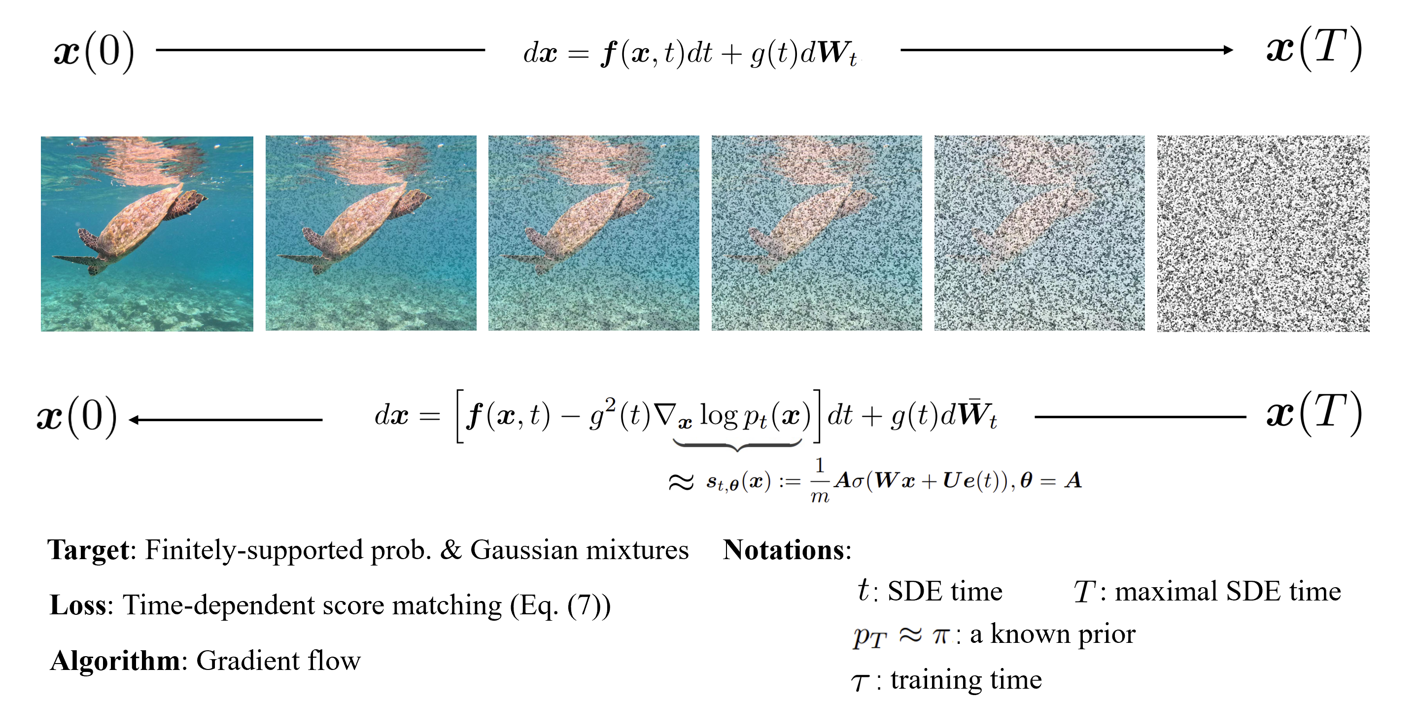
Since DMs/SGMs have already grown into a large family of generative models with an enormous number of variants, there are various ways to define the parameterization of diffusion models. Here, we adopt (one of) the most fundamental architectures proposed in [54], where the forward perturbation and reverse sampling process are both implemented by a joint group of coupled (stochastic) differential equations. See Figure 1 for an illustration of the problem formulation.
Forward perturbation.
We start with the setting of unsupervised learning. Given an unlabeled dataset with the sample , where denotes the underlying (ground truth or target) distribution, the forward diffusion process is defined as
| (1) |
Here, the drift coefficient is a time-dependent vector-valued function, and the diffusion coefficient is a scalar function, and denotes the standard Wiener process (a.k.a., Brownian motion). The SDE (1) has a unique, strong solution under certain regularity conditions (i.e., globally Lipschitz coefficients in both state and time; see [31]). From now on, we denote by the marginal distribution of , and let be the (perturbation) transition kernel from to , with as the time horizon. By appropriately selecting and , one can force the SDE (1) to converge to a prior distribution (typically a Gaussian). Common examples include the (time-rescaled) Ornstein–Uhlenbeck (OU) process,222The OU process is the unique time-homogeneous Markov process which is also a Gaussian process, with the stationary distribution as the standard Gaussian distribution. which is a special case of the linear version of (1):
| (2) |
Reverse sampling.
According to [1] and [54], both the following reverse-time SDE and probability flow ODE share the same marginal distribution as the forward-time SDE (1):
| (3) | ||||
| (4) |
where is a standard Wiener process when time flows backwards from to , and is an infinitesimal negative time step. With the initial condition , where is a known prior distribution such as the Gaussian noise, one can (numerically) solve (3) or (4) to transform noises into samples from , which is exactly the goal of generative modeling.
Loss objectives.
The only remaining task is to estimate the unknown (Stein) score function . This is achieved by minimizing the following weighted sum of denoising score matching ([57]) objectives:
| (5) |
with , where denotes the uniform distribution over , and is a weighting function, which is typically selected as
| (6) |
according to ([54]). The score function is time-dependent and can be parameterized as a neural network (encoded with the time information) such as the U-net([37]) architecture commonly applied in the field of image segmentation. Alternatively, one can also define the time-dependent score matching loss
| (7) |
which is equivalent to (5) up to a constant independent of by [57, 49].
In practice, expectations in the objective (5) can be respectively estimated with empirical means over time steps in , data samples from and , which is efficient when the drift coefficient is linear. Specifically, if the forward-time SDE takes the form of (2), the transition kernel has a closed form ([40])
| (8) |
where denotes the multivariate Gaussian distribution evaluated at with the expectation and covariance , and , .
Training.
We aim to investigate the gradient flow training dynamics over the empirical loss
| (9) |
where is the Monte-Carlo estimation of defined in (5) on the training dataset,333Recall the dataset , and we take for convenience. with an auxiliary gradient flow over the population loss
| (10) |
In both cases, the weighting function is selected as in (6). Denote the score function learned at the training time evaluated at the SDE time with respect to the empirical loss and population loss as and , respectively. The corresponding density functions, denoted by and , are obtained by solving
| (11) |
and then normalizing, respectively.
Score networks.
We parameterize the score function as the following random feature model
| (12) |
where is the ReLU activation function, is the trainable parameter, while and are randomly initialized and frozen during training, and is the embedding function concerning the time information. Assume that , and are i.i.d. sampled from an underlying distribution . Then, as , we get
| (13) |
with and . By the positive homogeneity property of the ReLU activation, we can assume that w.l.o.g.
One can view as a continuous version of the random feature model. Correspondingly, the optimal solution is denoted as when replacing the parameterized score function in the loss objective (5) or (7) by . Define the kernel
and let be the induced reproducing kernel Hilbert space (RKHS; [2]), we have if the RKHS norm , and the corresponding discrete version can be defined by the empirical average, i.e., .
Remark 1.
There are more modern and complex mathematical tools such as neural tangent kernels (NTKs) and mean fields that can be selected as the score networks. Employing these modern tools is valuable at least for theoretical completeness and we leave these as the future work.444For example, the extension to NTKs is possible, since the training of random feature models follows a specific NTK regime (only the last layer is updated) in the output space (instead of the parameter space), which can be properly analyzed in the infinite-width regime.
The goal is to measure and bound the generalization error evolving with the gradient flow training dynamics (9) between the learned distribution and target distribution, using the common Kullback–Leibler (KL) divergence.
Definition 1 (KL divergence).
Given two distributions and , the KL divergence from to is defined as .
Based on the above definitions, the generalization gap along the gradient flow training dynamics (9) is formulated as , which is only a function of the training time . The goal is to estimate .555Here, we aim at the density estimation characterization. This is different from [32], where the equivalence of learned and target data manifolds (support sets) is studied.
3.2 Main Results
In this section, we state the main results of the generalization capability of the (score-based) diffusion models and how it evolves as the training proceeds. Based on the formulation in Section 3.1, we theoretically derive several upper bounds to estimate under different settings. The results cover both the positive and negative aspects: in the data-independent setting where the target distribution has finite support, the generalization gap is proved to be small; while in the data-dependent setting where the target distribution possesses shift modes, the generalization is adversely affected by the modes’ distance.
3.2.1 Data-Independent Generalization Gap
In this section, we provide the characterization of the generalization capability for diffusion models given a target distribution defined on a finite domain. Generally, the KL divergence from the learned distribution at the training time to the target distribution can be estimated as follows.
Theorem 1.
Suppose that the target distribution is continuously differentiable and has a compact support set, i.e., is uniformly bounded, and there exists a reproducing kernel Hilbert space (RKHS) (:=) such that . Assume that the initial loss, trainable parameters, the embedding function and weighting function are all bounded. Then for any , , with the probability of at least , we have
where hides the term , the polynomials of , finite RKHS norms and universal positive constants only depending on .
Remark 2.
Since is compactly supported, the target score function is also defined on a compact domain. According to [12, 13], is contained in the Barron function space with a finite Barron norm, and hence in a certain RKHS with a finite RKHS norm. Therefore, it is reasonable to require that the global minimizer or is also contained in some RKHS.
Proof sketch.
Theorem 1 is proved via the following procedure.
-
1.
According to Theorem 1 in [49], the KL divergence on the left-hand side can be upper bounded by the population loss of the trained model up to a small error. That is,
(14) - 2.
-
3.
can be estimated via a similar argument as in [24] (Lemma 48).
-
4.
can be upper bounded via a standard analysis on the gradient flow dynamics over convex objectives.
-
5.
can be reduced as the norm product of , and their gap, then
-
(a)
the former can be bounded with a square-root rate growth via a general norm estimate of parameters trained under the gradient flow dynamics;
-
(b)
the latter can be estimated by the Rademacher complexity (see e.g., Chapter 26 in [43]).
-
(a)
Combining all above gives the desired result. The detailed proof is found in Appendix A.1.
Discussion on error bounds.
The three error terms are further analyzed as follows.
-
•
The first term is the main error, which implies an early-stopping generalization gap. In fact, if one selects an early-stopping time as , and let , we have
(16) - •
-
•
The third term is exponentially small in since (e.g. the Gaussian density) is log-Sobolev, according to a classical result in e.g. [55] (Theorem 3.20, Theorem 3.24 and Remark 3.26).
Remark 3.
In practice, it is common to use the test error to evaluate the generalization performance. For diffusion models, a straightforward approach is to compute the negative log-likelihood (averaged in bits/dim; equivalent to the KL divergence) on the test dataset during training with the instantaneous change-of-variable formula ([8]) and probability flow ODE (defined in (4)), where the true score function is replaced by .
Remark 4.
Previous literature has established similar bounds for bias potential models ([66]) and GANs ([67]). Theorem 1 extends the corresponding results to the setting of diffusion models. Furthermore, this upper bound is finer in the sense that it incorporates the information regarding the model capacity (the hidden dimension in this case), which shows that more parameters benefit the learning and generalization, as expected.
3.2.2 Data-Dependent Generalization Gap
In Section 3.2.1, we derive estimates on the generalization error for diffusion models along the training dynamics, where the target distribution is assumed to be finitely supported. In reality, this is often not the case, where target distributions usually possess distant multi-modes, from simple Gaussian mixtures to complicated Boltzmann distributions of physical systems ([29, 30]). Under these settings, the above analysis in Section 3.2.1 can not directly apply since the data domain is unbounded. It remains a problem to quantitatively characterize the generalization behavior of diffusion models given these target distributions with distant multi-modes or modes shift.
To provide a fine-grained demonstration of the generalization capability of diffusion models when applied to learn distributions with distant multi-modes, as an illustrating example, the Gaussian mixture with two modes is selected as the target distribution.
Theorem 2.
Suppose the target distribution is a one-dimensional 2-mode Gaussian mixture: , where , with are all constants. Under the conditions of Theorem 1 (except the uniform boundness of inputs), we have
where , hides the polynomials of , finite RKHS norms and universal positive constants only depending on .
Proof sketch.
Theorem 2 is proved following a similar procedure with Theorem 1, except the input data does not have a uniform bound here. This problem mainly affects the last step (5 (b)) in the proof sketch of Theorem 1, and can be handled by using the fact
| (17) |
given the target Gaussian mixture distribution. The detailed proof is found in Appendix A.2.
Remark 5.
Theorem 2 indicates that, even for a simple target distribution (e.g. a one-dimensional 2-mode Gaussian mixture), the generalization error of diffusion models can be polynomially large regarding the modes’ distance. Although Theorem 2 provides only an upper bound, the modes shift effect holds due to the model-target inconsistency (the last paragraph in Appendix A.2) and the following consistent experiments (Section 4.1.2).
4 Numerical Verifications
In this section, we numerically verify the previous theoretical results and insights (early-stopping generalization and modes shift effect) on both synthetic datasets and real-world datasets.
4.1 Simulations on Synthetic Datasets
4.1.1 Early-Stopping Generalization
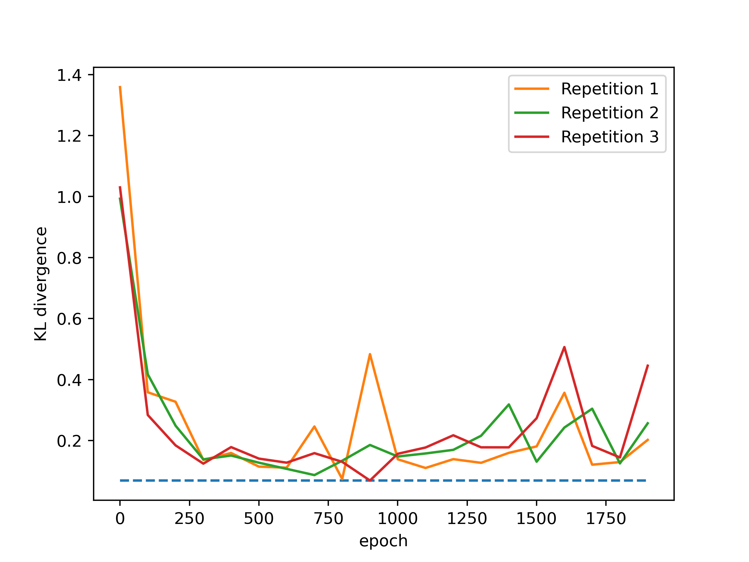
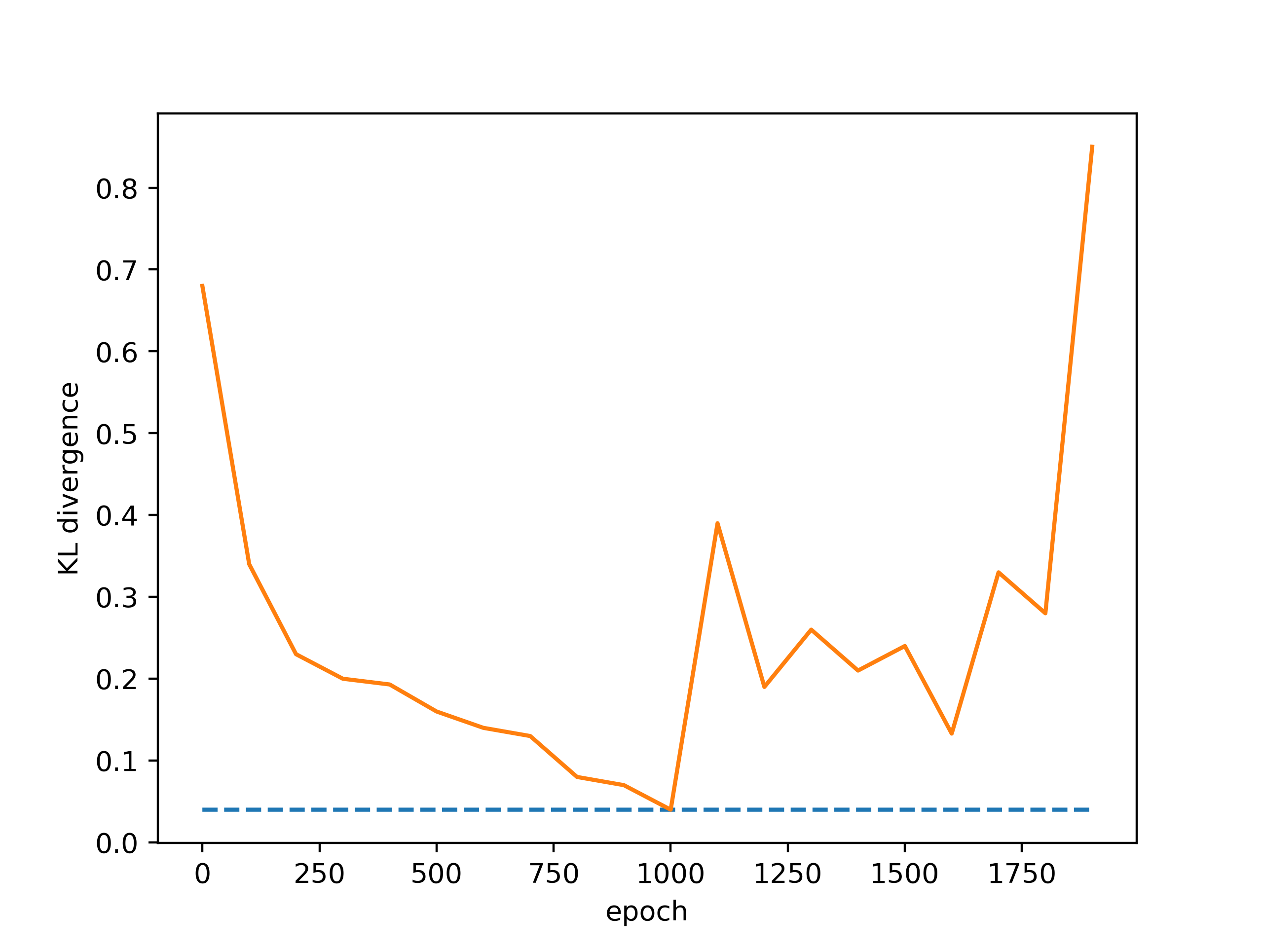
First, we illustrate the early-stopping generalization gap established in Theorem 1. We select the one-hidden-layer neural network with Swish activations as the score network, which is trained using the SGD optimizer with a fixed learning rate . The target distribution is set to be a one-dimensional 2-mode Gaussian mixture with the modes’ distance equalling 6, and the number of data samples is 1000. We measure the KL divergence from the trained model to the target distribution along with the training epochs.
From Figure 3, one can observe that the KL divergence achieves its minimum at approximately the -th training epoch, and it starts to increase after this turning point. The experimental results are consistent with Theorem 1 (over multiple runs), which states that there exist early-stopping times when diffusion models can generalize well, indicating the effectiveness of our upper bound. Further, the KL divergence begins to oscillate after the minimum point, which may suggest a phase transition in the training dynamics, and the transition point is around the (optimal) early-stopping time.
4.1.2 Modes Shift Effect
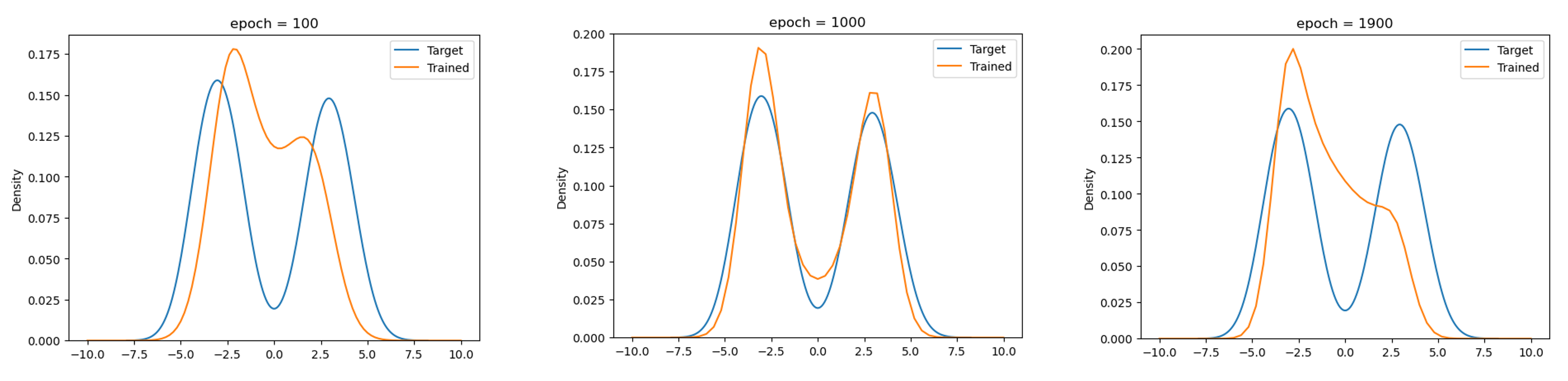
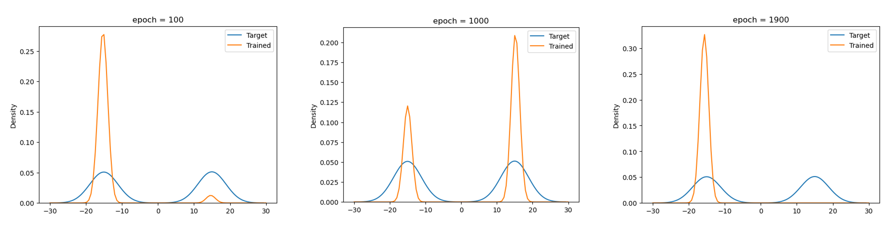
Next, we numerically test the relationship between the modes’ distance and generalization (density estimation) performance. All the configurations remain the same as Section 4.1.1, except that the target Gaussian mixtures have different modes’ distances.
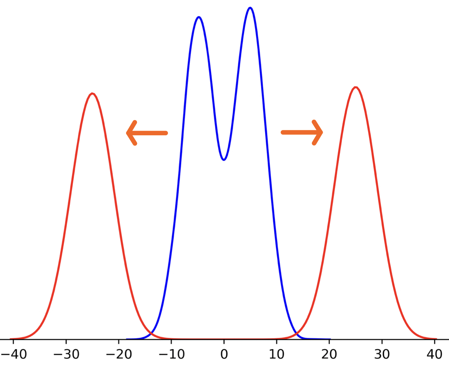
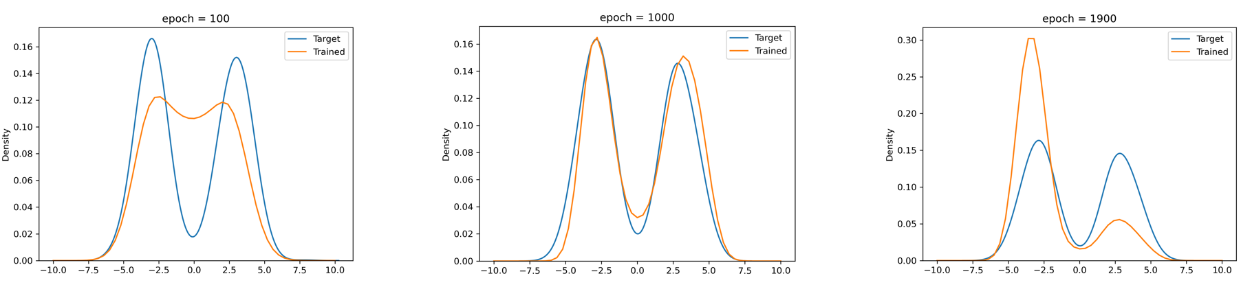
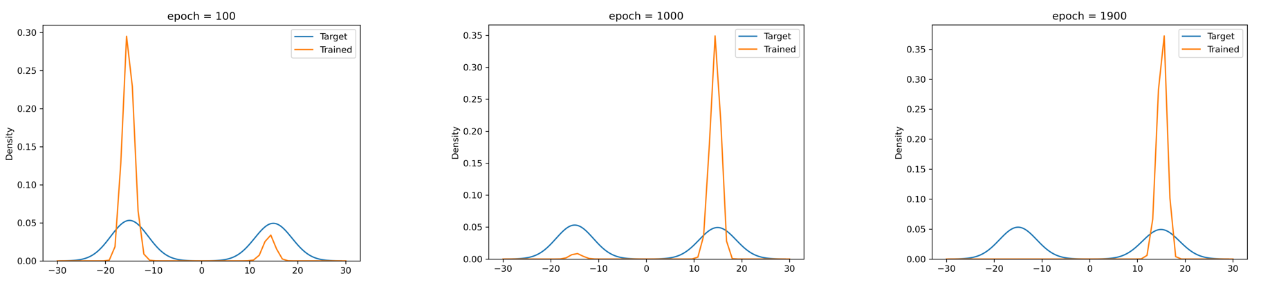
In Figure 4, the modeled distributions exhibit the following two-stage dynamics: (i) first gradually fitting the two modes (epoch ); (ii) then diverging (epoch ). This aligns with the KL divergence dynamics (Figure 3) and again verifies the corresponding theoretical results (Theorem 1). However, Figure 5 shows that when the modes are distant from each other, there is difficulty in the learning process. In Figure 5, the optimal generalization is achieved at epoch , but is still far from well generalizing. As the training proceeds, the learned model is almost always a single-mode distribution (epoch ). This phenomenon is aligned with the results established in Theorem 2, which states that when there are distant modes in the target distribution, the generalization performance is relatively poor.
4.2 Simulations on Real-World Datasets
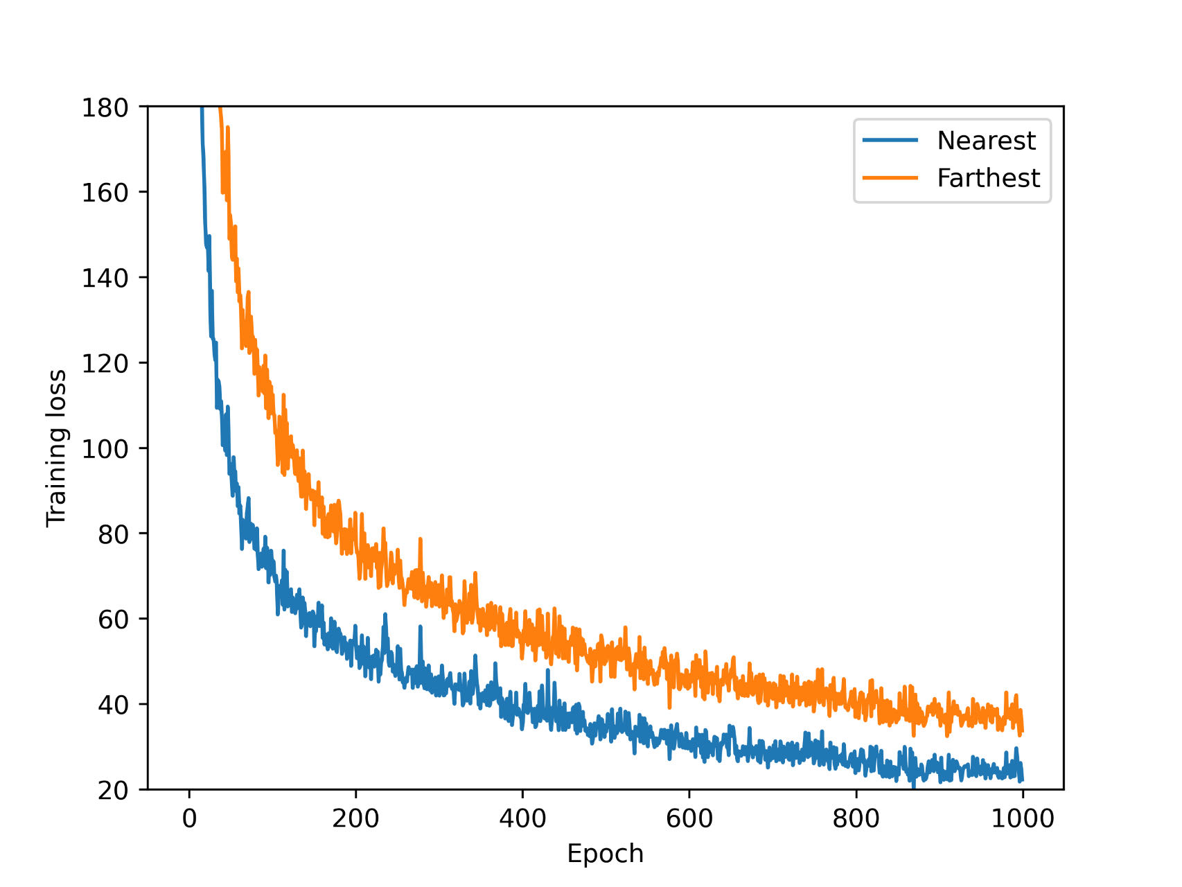
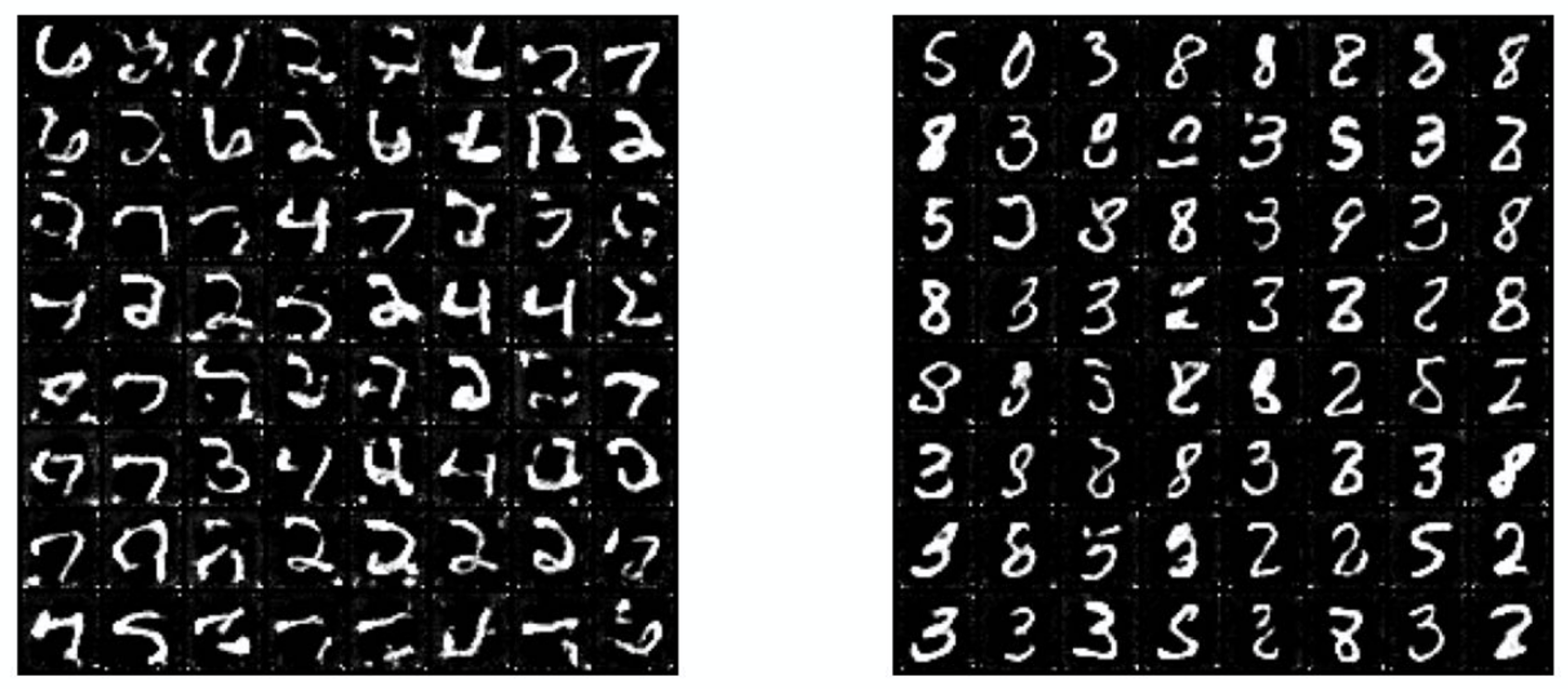
In this subsection, we verify our results on the MNIST dataset using the standard U-net architecture as the score network, which suggests that the adverse effect of modes shift on the generalization performance of diffusion models also appears in general.
The setup is as follows. First, we perform a -means clustering on ( denote the MNIST dataset) to get , and as the center of , . Let , and . is similarly constructed by indices. Then, by randomly selecting the same number of data samples and using the same configuration, we train two separate diffusion models on and , respectively, and then perform inference (sampling). The training loss curves and sampling results are shown in Figure 6 and Figure 7, respectively. One can observe a significant performance gap: the diffusion model trained on appears a higher learning loss and worse sampling quality compared to those of .
4.3 Discussion
We compare the results developed in this work with former corresponding literature as follows:
-
•
The previous work [21] also studied the adverse effect of modes shift, which particularly reported a contrastive simulation indicating the degraded performance when modeling Gaussian mixtures with the increasing distance between modes (see Figure 2 in [21] and compare with Figure 4 and Figure 5). However, the results therein are established and tested under the “pure” score matching setting, without the denoising or time-dependent dynamics. As a comparison, Theorem 2 establishes a theoretical estimate on the generalization gap for diffusion models that requires denoising, and this upper bound directly depends on the distance between modes of target distributions, instead of a circuitous characterization in [21] to attribute the difficulty of learning modes shift to increased isoperimetry of corresponding target distributions.
-
•
Similar adverse effect of modes shift has also been theoretically analyzed and numerically verified on recurrent neural networks (RNNs), see e.g., [23, 24]. There, the modes shift is understood as a type of long-term memory. This is the phenomenon of the “curse of memory”: When there is long-term memory in the target, it requires a large number of parameters for the approximation. Meanwhile, the training process will suffer from severe slowdowns. Both of these effects can be exponentially more pronounced with increasing memory or modes shift.
-
•
The very recent work [42] also considered the problem of learning Gaussian mixtures using the denoising diffusion probabilistic model (DDPM) objective, but under a teacher-student setting. That is, given the Gaussian mixtures target, [42] parametrized the score network model in the same form of the score function target, with the goal to identify true parameters. Consequently, there are all positive convergence results developed in [42], despite that the time and sample complexity increases with the distance between modes. As a comparison, Theorem 2 adopts a pre-selected score network model without incorporating any information from the ground truth, and hence establish negative results concerning the modes shift. In fact, if the goal is to identify only true positions of the target Gaussian mixture (this is exactly the setting of [42]), the teacher-student setup seems not necessary (see Figure 5, where the true position is also learned efficiently using the one-hidden-layer Swish neural network as the score network, but the modes are always weighed incorrectly). In addition, [42] did not take the whole denoising dynamics into account. That is, the gradient descent (GD) analysis therein was performed on the denoising score matching objective successively at only two time stages: a larger (“high noise”) and a smaller (“low noise”), which is often not the case in practice.
5 Conclusion
In this paper, we provide a theoretical analysis of the fundamental generalization aspect of training diffusion models under both the data-independent and data-dependent settings, and early-stopping estimates of the generalization gap along the training dynamics are derived. Quantitatively, the data-independent results indicate a polynomially small generalization error that escapes from the curse of dimensionality, while the data-dependent results suggest the adverse effect of modes shift in target distributions. Numerical simulations have illustrated and verified these theoretical analyses. This work forms a basic starting point for understanding the intricacies of modern deep generative modeling and corresponding central concerns such as memorization, privacy, and copyright arising from practical applications and business products. More broadly, the approach here may have the potential to be extended to other variants in the diffusion models family, including a general SDE-based design space ([20]), consistency models ([48]), rectified flows ([27, 26]), Schrödinger bridges ([59, 56, 10, 44, 47, 25]), etc. These are certainly worthy of future exploration.
Acknowledgements
We would like to thank Dr. Hongkang Yang for helpful discussions, and all the reviewers’ valuable feedback and insightful suggestions to improve this work.
References
- [1] Brian D. O. Anderson. Reverse-time diffusion equation models. Stochastic Processes and their Applications, 12(3):313–326, 1982.
- [2] Nachman Aronszajn. Theory of reproducing kernels. Transactions of the American Mathematical Society, 68(3):337–404, 1950.
- [3] Jacob Austin, Daniel D. Johnson, Jonathan Ho, Daniel Tarlow, and Rianne van den Berg. Structured denoising diffusion models in discrete state-spaces. Advances in Neural Information Processing Systems, 34:17981–17993, 2021.
- [4] Omri Avrahami, Dani Lischinski, and Ohad Fried. Blended diffusion for text-driven editing of natural images. In Proceedings of the IEEE/CVF Conference on Computer Vision and Pattern Recognition, pages 18208–18218, 2022.
- [5] Nicholas Carlini, Jamie Hayes, Milad Nasr, Matthew Jagielski, Vikash Sehwag, Florian Tramer, Borja Balle, Daphne Ippolito, and Eric Wallace. Extracting training data from diffusion models. In USENIX Security Symposium, pages 5253–5270, 2023.
- [6] Nicholas Carlini, Daphne Ippolito, Matthew Jagielski, Katherine Lee, Florian Tramer, and Chiyuan Zhang. Quantifying memorization across neural language models. In International Conference on Learning Representations, 2023.
- [7] Hongrui Chen, Holden Lee, and Jianfeng Lu. Improved analysis of score-based generative modeling: User-friendly bounds under minimal smoothness assumptions. International Conference on Machine Learning, 202:4735–4763, 2023.
- [8] Ricky T. Q. Chen, Yulia Rubanova, Jesse Bettencourt, and David K. Duvenaud. Neural ordinary differential equations. Advances in Neural Information Processing Systems, 31:6571–6583, 2018.
- [9] Sitan Chen, Sinho Chewi, Jerry Li, Yuanzhi Li, Adil Salim, and Anru Zhang. Sampling is as easy as learning the score: Theory for diffusion models with minimal data assumptions. In International Conference on Learning Representations, 2023.
- [10] Valentin De Bortoli, James Thornton, Jeremy Heng, and Arnaud Doucet. Diffusion Schrödinger bridge with applications to score-based generative modeling. Advances in Neural Information Processing Systems, 34:17695–17709, 2021.
- [11] Tim Dockhorn, Tianshi Cao, Arash Vahdat, and Karsten Kreis. Differentially private diffusion models. Transactions on Machine Learning Research, 2023.
- [12] Weinan E, Chao Ma, and Lei Wu. A priori estimates of the population risk for two-layer neural networks. Communications in Mathematical Sciences, 17(5):1407–1425, 2019.
- [13] Weinan E, Chao Ma, and Lei Wu. The Barron space and the flow-induced function spaces for neural network models. Constructive Approximation, 55(1):369–406, 2022.
- [14] Sahra Ghalebikesabi, Leonard Berrada, Sven Gowal, Ira Ktena, Robert Stanforth, Jamie Hayes, Soham De, Samuel L Smith, Olivia Wiles, and Borja Balle. Differentially private diffusion models generate useful synthetic images. In International Workshop on Trustworthy Federated Learning in Conjunction with IJCAI, 2023.
- [15] Shansan Gong, Mukai Li, Jiangtao Feng, Zhiyong Wu, and Lingpeng Kong. Diffuseq: Sequence to sequence text generation with diffusion models. In International Conference on Learning Representations, 2023.
- [16] Jonathan Ho, Ajay Jain, and Pieter Abbeel. Denoising diffusion probabilistic models. Advances in Neural Information Processing Systems, 33:6840–6851, 2020.
- [17] Daniel Hsu, Clayton H. Sanford, Rocco Servedio, and Emmanouil Vasileios Vlatakis-Gkaragkounis. On the approximation power of two-layer networks of random ReLUs. Conference on Learning Theory, 134:2423–2461, 2021.
- [18] Hailong Hu and Jun Pang. Membership inference of diffusion models. arXiv preprint arXiv:2301.09956, 2023.
- [19] Matthew Jagielski, Om Thakkar, Florian Tramer, Daphne Ippolito, Katherine Lee, Nicholas Carlini, Eric Wallace, Shuang Song, Abhradeep Guha Thakurta, Nicolas Papernot, and Chiyuan Zhang. Measuring forgetting of memorized training examples. In International Conference on Learning Representations, 2023.
- [20] Tero Karras, Miika Aittala, Timo Aila, and Samuli Laine. Elucidating the design space of diffusion-based generative models. Advances in Neural Information Processing Systems, 35:26565–26577, 2022.
- [21] Frederic Koehler, Alexander Heckett, and Andrej Risteski. Statistical efficiency of score matching: The view from isoperimetry. In International Conference on Learning Representations, 2023.
- [22] Haoying Li, Yifan Yang, Meng Chang, Shiqi Chen, Huajun Feng, Zhihai Xu, Qi Li, and Yueting Chen. Srdiff: Single image super-resolution with diffusion probabilistic models. Neurocomputing, 479:47–59, 2022.
- [23] Zhong Li, Jiequn Han, Weinan E, and Qianxiao Li. On the curse of memory in recurrent neural networks: Approximation and optimization analysis. In International Conference on Learning Representations, 2021.
- [24] Zhong Li, Jiequn Han, Weinan E, and Qianxiao Li. Approximation and optimization theory for linear continuous-time recurrent neural networks. Journal of Machine Learning Research, 23(42):1–85, 2022.
- [25] Guan-Horng Liu, Arash Vahdat, De-An Huang, Evangelos Theodorou, Weili Nie, and Anima Anandkumar. I2SB: Image-to-image Schrödinger bridge. International Conference on Machine Learning, 202:22042–22062, 2023.
- [26] Qiang Liu. Rectified flow: A marginal preserving approach to optimal transport. arXiv preprint arXiv:2209.14577, 2022.
- [27] Xingchao Liu, Chengyue Gong, and Qiang Liu. Flow straight and fast: Learning to generate and transfer data with rectified flow. In International Conference on Learning Representations, 2023.
- [28] Tomoya Matsumoto, Takayuki Miura, and Naoto Yanai. Membership inference attacks against diffusion models. In IEEE Security and Privacy Workshops, pages 77–83, 2023.
- [29] Laurence Illing Midgley, Vincent Stimper, Gregor N. C. Simm, Bernhard Schölkopf, and José Miguel Hernández-Lobato. Flow annealed importance sampling bootstrap. In International Conference on Learning Representations, 2023.
- [30] Frank Noé, Simon Olsson, Jonas Köhler, and Hao Wu. Boltzmann generators: Sampling equilibrium states of many-body systems with deep learning. Science, 365(6457):eaaw1147, 2019.
- [31] Bernt Øksendal. Stochastic Differential Equations. Springer, 2003.
- [32] Jakiw Pidstrigach. Score-based generative models detect manifolds. Advances in Neural Information Processing Systems, 35:35852–35865, 2022.
- [33] Vadim Popov, Ivan Vovk, Vladimir Gogoryan, Tasnima Sadekova, and Mikhail Kudinov. Grad-tts: A diffusion probabilistic model for text-to-speech. International Conference on Machine Learning, 139:8599–8608, 2021.
- [34] Aditya Ramesh, Prafulla Dhariwal, Alex Nichol, Casey Chu, and Mark Chen. Hierarchical text-conditional image generation with clip latents. arXiv preprint arXiv:2204.06125, 2022.
- [35] Kashif Rasul, Calvin Seward, Ingmar Schuster, and Roland Vollgraf. Autoregressive denoising diffusion models for multivariate probabilistic time series forecasting. International Conference on Machine Learning, 139:8857–8868, 2021.
- [36] Robin Rombach, Andreas Blattmann, Dominik Lorenz, Patrick Esser, and Björn Ommer. High-resolution image synthesis with latent diffusion models. In Proceedings of the IEEE/CVF Conference on Computer Vision and Pattern Recognition, pages 10684–10695, 2022.
- [37] Olaf Ronneberger, Philipp Fischer, and Thomas Brox. U-net: Convolutional networks for biomedical image segmentation. In Medical Image Computing and Computer-Assisted Intervention, pages 234–241. Springer, 2015.
- [38] Chitwan Saharia, William Chan, Saurabh Saxena, Lala Li, Jay Whang, Emily Denton, Seyed Kamyar Seyed Ghasemipour, Raphael Gontijo-Lopes, Burcu Karagol Ayan, Tim Salimans, Jonathan Ho, David J. Fleet, and Mohammad Norouzi. Photorealistic text-to-image diffusion models with deep language understanding. Advances in Neural Information Processing Systems, 35:36479–36494, 2022.
- [39] Chitwan Saharia, Jonathan Ho, William Chan, Tim Salimans, David J. Fleet, and Mohammad Norouzi. Image super-resolution via iterative refinement. IEEE Transactions on Pattern Analysis and Machine Intelligence, 45(4):4713–4726, 2023.
- [40] Simo Särkkä and Arno Solin. Applied Stochastic Differential Equations, volume 10. Cambridge University Press, 2019.
- [41] Vikash Sehwag, Caner Hazirbas, Albert Gordo, Firat Ozgenel, and Cristian Canton. Generating high fidelity data from low-density regions using diffusion models. In Proceedings of the IEEE/CVF Conference on Computer Vision and Pattern Recognition, pages 11492–11501, 2022.
- [42] Kulin Shah, Sitan Chen, and Adam Klivans. Learning mixtures of gaussians using the DDPM objective. Advances in Neural Information Processing Systems, 36, 2023.
- [43] Shai Shalev-Shwartz and Shai Ben-David. Understanding Machine Learning: From Theory to Algorithms. Cambridge University Press, 2014.
- [44] Yuyang Shi, Valentin De Bortoli, Andrew Campbell, and Arnaud Doucet. Diffusion Schrödinger bridge matching. Advances in Neural Information Processing Systems, 36, 2023.
- [45] Jascha Sohl-Dickstein, Eric Weiss, Niru Maheswaranathan, and Surya Ganguli. Deep unsupervised learning using nonequilibrium thermodynamics. International Conference on Machine Learning, 37:2256–2265, 2015.
- [46] Gowthami Somepalli, Vasu Singla, Micah Goldblum, Jonas Geiping, and Tom Goldstein. Diffusion art or digital forgery? investigating data replication in diffusion models. In Proceedings of the IEEE/CVF Conference on Computer Vision and Pattern Recognition, pages 6048–6058, 2023.
- [47] Vignesh Ram Somnath, Matteo Pariset, Ya-Ping Hsieh, Maria Rodriguez Martinez, Andreas Krause, and Charlotte Bunne. Aligned diffusion Schrödinger bridges. Conference on Uncertainty in Artificial Intelligence, 216:1985–1995, 2023.
- [48] Yang Song, Prafulla Dhariwal, Mark Chen, and Ilya Sutskever. Consistency models. International Conference on Machine Learning, 202:32211–32252, 2023.
- [49] Yang Song, Conor Durkan, Iain Murray, and Stefano Ermon. Maximum likelihood training of score-based diffusion models. Advances in Neural Information Processing Systems, 34:1415–1428, 2021.
- [50] Yang Song and Stefano Ermon. Generative modeling by estimating gradients of the data distribution. Advances in Neural Information Processing Systems, 32, 2019.
- [51] Yang Song and Stefano Ermon. Improved techniques for training score-based generative models. Advances in Neural Information Processing Systems, 33:12438–12448, 2020.
- [52] Yang Song, Sahaj Garg, Jiaxin Shi, and Stefano Ermon. Sliced score matching: A scalable approach to density and score estimation. Uncertainty in Artificial Intelligence Conference, 115:574–584, 2020.
- [53] Yang Song, Liyue Shen, Lei Xing, and Stefano Ermon. Solving inverse problems in medical imaging with score-based generative models. In International Conference on Learning Representations, 2022.
- [54] Yang Song, Jascha Sohl-Dickstein, Diederik P. Kingma, Abhishek Kumar, Stefano Ermon, and Ben Poole. Score-based generative modeling through stochastic differential equations. In International Conference on Learning Representations, 2021.
- [55] Ramon Van Handel. Probability in high dimension. Lecture Notes (Princeton University), 2014.
- [56] Francisco Vargas, Pierre Thodoroff, Austen Lamacraft, and Neil Lawrence. Solving Schrödinger bridges via maximum likelihood. Entropy, 23(9):1134, 2021.
- [57] Pascal Vincent. A connection between score matching and denoising autoencoders. Neural Computation, 23(7):1661–1674, 2011.
- [58] Nikhil Vyas, Sham M. Kakade, and Boaz Barak. On provable copyright protection for generative models. International Conference on Machine Learning, 202:35277–35299, 2023.
- [59] Gefei Wang, Yuling Jiao, Qian Xu, Yang Wang, and Can Yang. Deep generative learning via Schrödinger bridge. International Conference on Machine Learning, 139:10794–10804, 2021.
- [60] Jay Zhangjie Wu, Yixiao Ge, Xintao Wang, Stan Weixian Lei, Yuchao Gu, Yufei Shi, Wynne Hsu, Ying Shan, Xiaohu Qie, and Mike Zheng Shou. Tune-a-video: One-shot tuning of image diffusion models for text-to-video generation. In Proceedings of the IEEE/CVF International Conference on Computer Vision, pages 7623–7633, 2023.
- [61] Lei Wu and Weijie J. Su. The implicit regularization of dynamical stability in stochastic gradient descent. International Conference on Machine Learning, 202:37656–37684, 2023.
- [62] Yixin Wu, Ning Yu, Zheng Li, Michael Backes, and Yang Zhang. Membership inference attacks against text-to-image generation models. arXiv preprint arXiv:2210.00968, 2022.
- [63] Tian Xie, Xiang Fu, Octavian-Eugen Ganea, Regina Barzilay, and Tommi S. Jaakkola. Crystal diffusion variational autoencoder for periodic material generation. In International Conference on Learning Representations, 2022.
- [64] Minkai Xu, Lantao Yu, Yang Song, Chence Shi, Stefano Ermon, and Jian Tang. Geodiff: A geometric diffusion model for molecular conformation generation. In International Conference on Learning Representations, 2022.
- [65] Hongkang Yang. A mathematical framework for learning probability distributions. Journal of Machine Learning, 1(4):373–431, 2022.
- [66] Hongkang Yang and Weinan E. Generalization and memorization: The bias potential model. Mathematical and Scientific Machine Learning, 145:1013–1043, 2022.
- [67] Hongkang Yang and Weinan E. Generalization error of GAN from the discriminator’s perspective. Research in the Mathematical Sciences, 9(1):1–31, 2022.
- [68] Ruihan Yang, Prakhar Srivastava, and Stephan Mandt. Diffusion probabilistic modeling for video generation. Entropy, 25(10):1469, 2023.
- [69] Jongmin Yoon, Sung Ju Hwang, and Juho Lee. Adversarial purification with score-based generative models. International Conference on Machine Learning, 139:12062–12072, 2021.
- [70] Chiyuan Zhang, Daphne Ippolito, Katherine Lee, Matthew Jagielski, Florian Tramèr, and Nicholas Carlini. Counterfactual memorization in neural language models. Advances in Neural Information Processing Systems, 36, 2023.
Appendix A Technical Results and Proofs
A.1 Data-Independent Generalization Gap
To derive the theorem for the generalization error of this score-based generative model, we first give the following lemmas.
Lemma 1 (Forward perturbation estimates).
Consider the forward diffusion process with the linear drift coefficient (2). For any , , with the probability of at least , we have
| (18) |
where .
Proof.
When the drift coefficient is linear to , i.e., , the transition kernel has a closed form (8)
| (19) |
with , . Hence, we have
| (20) |
For any , , we have
Let , we get
| (21) |
Hence, for any with , with the probability of at least , we have
| (22) |
with . The proof is completed. ∎
Lemma 2 (Theorem 1 in [49]).
We have
Lemma 3.
Both of the loss objectives and are quadratic (and hence convex).
Proof.
The convexity arises from the following points: (i) The score matching loss objectives (defined in (7)) and are -metrics between the score network model and target score function; (ii) The score networks are defined as random feature models (see (12) and (3.1)) that are linear to trainable parameters. Therefore, using some trace techniques and basic variational calculations, it is not hard to derive the fact that the loss objectives are quadratic and hence convex with respect to trainable parameters.
(1) For , recall that , and let , , , we have
Since for any , we have
we further get
where
Here, is a positive semi-definite matrix, since for any . Notice that for any ,
where denotes the Kronecker product. Hence
| (23) |
is a quadratic function. It is straightforward to show that the eigenvalues of are the same as but with multiplicity,666 In fact, if , have the eigenvalues , , respectively, the eigenvalues of are , , . This is due to the following argument. By Jordan–Chevalley decomposition, there exist invertible matrices such that , , where are upper triangular matrices. Therefore, we have That is, the matrices and are similar. Notice that is still an upper triangular matrix with diagonal elements , , , we obatain the desired result. implying that is also positive semi-definite. Therefore,
is positive semi-definite, i.e., the loss is convex with respect to trainable parameters.
(2) For , notice that
Let , , , we get
Then for any , by symmetry we have
where
This yields
| (24) |
and
hence the functional is convex with respect to (given any positive weighting function ). The proof is completed. ∎
Since the weighting function is fixed in our analysis, we omit the notation without ambiguity in the following contents.
Lemma 4.
For any and , we have
Proof.
(1) For the loss objective , we define the Lyapunov function
Then, we have
where the last inequality holds since
By convexity, for any , it holds that
hence . We conclude that , or equivalently
Therefore, note that (let ), we obtain
which gives the desired estimate.
(2) For the loss objective , the argument is almost the same, except replacing the Lyapunov function by
and by . Note that and , we obtain
which completes the proof. ∎
Lemma 5.
Suppose that the loss objectives , , , are bounded at the initialization, then for any , we have
Proof.
It’s sufficient to prove , and the rest part follows similarly.
Since
applying Cauchy–Schwartz inequality yields
Thus, again by Cauchy–Schwartz inequality, for any , we have
By choosing , we have , hence , which completes the proof. ∎
Lemma 6 (Monte Carlo estimates).
Define the Monte Carlo error
| (25) |
Suppose that , and the trainable parameter and embedding function are both bounded. Then, given any , for any , , with the probability of at least , there exists such that
| (26) |
where hides universal positive constants only depending on .
Proof.
Fix any . According to Lemma 1, for any , , with the probability of at least , we have
| (27) |
Based on the representation (3.1), for any , with , , let with for , and
| (28) |
then . For , let
If is different from at only one component indexed by , we have
where (i) is from the triangle inequality, (ii) is due to the fact that for any , the triangle and Hölder’s inequality and (27), (iii) follows from the positive homogeneity property of the ReLU activation, and (iv) is due to the boundness of the trainable parameter and embedding function . By McDiarmid’s inequality (see e.g., Lemma 26.4 in [43]), for any , with the probability of at least , we have
| (29) | ||||
| (30) |
Since
| (31) | ||||
| (32) |
where (v) is due to Fubini’s theorem, and (ii), (iii), (iv) is the same as before. By the triangle inequality, Jensen’s inequality, (29) and (31), we obtain
| (33) |
which gives
Obviously, . The proof is completed. ∎
Now we are ready to prove the main theorem.
Proof of Theorem 1.
Based on Lemma 2, we have
To bound the term , we use the following decomposition:
According to Lemma 4, we obtain
The term can be further divided into
where is the Monte Carlo estimator of . By Lemma 6, for any , , with the probability of at least , it holds that
| (34) |
while Lemma 4 gives
and similarly,
Hence, for any , , with the probability of at least , it holds that
For the term , we have
Notice that
which gives
Here, the triangle inequality, Cauchy–Schwartz inequality, the fact that for any , Hölder’s inequality, the positive homogeneity property of the ReLU activation, and the boundness of the input data, embedding function and weighting function . Thus, we get
where the last inequality follows from Lemma 4. We further deduce that
where denotes the empirical distribution of . Note that
| (35) |
by Lemma 5 we get . For any , define the function space
where
Then, according to Theorem A.5 in [61], for any , with the probability at least over the choice of the dataset , it holds that
where denotes the (empirical) Rademacher complexity of on , and all the inequalities hold in the element-wise sense.
(i) For , according to Lemma A.6 in [61], we have
Note that
| (36) |
which yields
| (37) |
and hence
where . This gives
Let
according to Lemma 26.6 in [43], we get . Since
where the are independent random variables with the distribution , and obviously,
we have
and by symmetry
i.e., . According to Lemma 26.9 (contraction lemma) and Lemma 26.11 in [43], we have
Combining above, we obtain
Combining (i), (ii) and (iii), we obtain
which gives
| (38) | ||||
where hides universal positive constants only depending on .
Combining all above estimates yields
If one only focuses on the -dependence, i.e. the dependence on the model capacity and sample size, this upper bound can be further simplified as
where we assume for simplicity, and hides the term , the polynomials of and finite RKHS norms . The proof is completed. ∎
Approximation errors.
For the (universal) approximation, we discuss in two points:
-
•
First, the approximation is a separate problem that can be analyzed independently of training and generalization. While it is beyond the scope of current work, we have included the approximation error in the final estimates. When the approximation by random feature models fails, the generalization error is supposed to be significant.
-
•
In addition, the random feature model can approximate Lipschitz continuous functions on a compact domain (Theorem 6 in [17]). Notice that the forward diffusion process defines a random path contained in a rectangular domain with (use Lemma 1 and the boundness of inputs), one can apply Theorem 6 in [17] to bound (7) on the domain in to obtain approximation results for Lipschitz continuous target score functions.
A.2 Data-Dependent Generalization Gap
Lemma 7 (Forward perturbation estimates, Gaussian mixtures).
Suppose that is sampled from a one-dimensional 2-mode Gaussian mixture: , where , with are all constants. Then for any , , , with the probability of at least , we have
| (39) |
Proof.
Lemma 8 (Monte Carlo estimates, Gaussian mixtures).
Define the Monte Carlo error
| (42) |
Suppose that the trainable parameter and embedding function are both bounded, and is sampled from a one-dimensional 2-mode Gaussian mixture: , where , with are all constants. Then, given any , for any , , , with the probability of at least , there exists such that
| (43) |
where hides universal positive constants only depending on .
Proof.
Proof of Theorem 2.
Remark 6.
A standard variance is used here for convenience. In general, if as (e.g. a bounded var), similar analysis and results are supposed to hold. However, this is different when as , since the modes are not separated in this case, and we can not characterize modes shift by simply varying .
Remark 7.
Simply scaling down inputs seems not to resolve the adverse effect of modes shift, since the ground truth is unknown. One can use the input scale to approximate on toy datasets, but it is not that trivial in practice, particularly for real-world applications with multiple high-dimensional modes in varied scales.
The model-target inconsistency.
Informally, there is inconsistency between the score network model and target score function. In fact, given the target Gaussian mixture , the target score function is
which gives , and , . While the score network model is
where "" holds since by (40) (). Both and are linear functions, but they have unmatched scales in slopes and intercepts: and for , but both ’s for . That is, modeling Gaussian mixtures with large modes distances as random feature models is inconsistent.
Appendix B Additional Experiments
B.1 Early-Stopping Generalization
We illustrate the early-stopping generalization gap established in Theorem 1 using the Adam optimizer. All the configurations remain the same as Section 4.1 except that the learning rate is now .
From Figure 8, one can observe that the KL divergence achieves its minimum at the 1000th training epoch, and it starts to increase after this turning point. The plot is aligned with Theorem 1, which states that there exists an optimal early-stopping time when the model can generalize well, indicating the effectiveness of the upper bound. Further, the KL divergence begins to oscillate after the minimum point (1000th training epoch), which may suggest a phase transition in the KL divergence dynamics, and the transition point is around the optimal early-stopping time. The finding is aligned with SGD setting.
B.2 Modes Shift Effect
We further test the relationship between the modes’ distance and the generalization performance using the Adam optimizer under the same configurations.
In Figure 9 and Figure 10, it is shown that the training of modeled distributions exhibits the same two-stage dynamics as the SGD setting, indicating that the modes shift effect holds not particularly for a certain optimizer.
B.3 Model Capacity Dependency
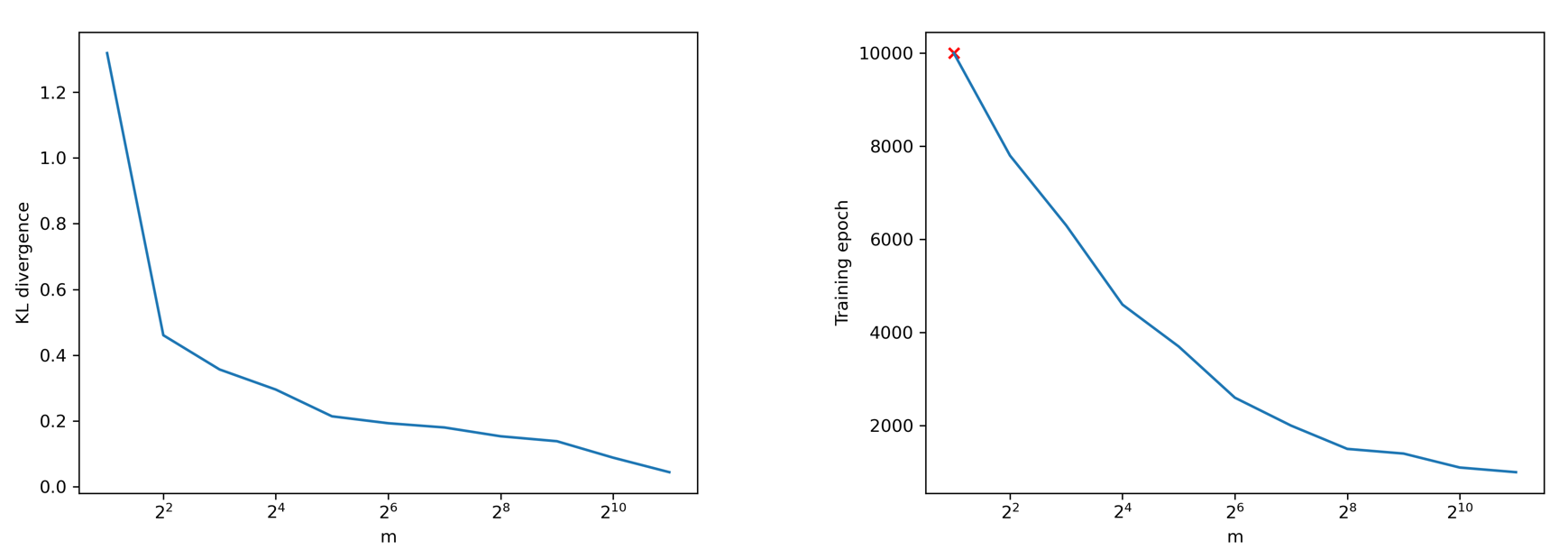
We also numerically study the dependency of generalization on the model capacity. Following the same configurations in Section 4.1.1, we conduct experiments for different hidden dimensions varying from to .
In Figure 11, the left plot shows the KL divergence from the trained distribution at the 1000th training epoch to the target distribution, and the right plot shows the time duration of the modeled distribution to generalize. Here, the generalization criterion we select is , and we stop training at epoch . Both the two plots in Figure 11 indicate that increasing model capacity benefits the generalization, which also verifies the corresponding theoretical results (-dependency in Theorem 1 and Theorem 2).