Abstract

Historically, the interpolation of large geophysical datasets has been tackled using methods like Optimal Interpolation (OI) or model-based data assimilation schemes. However, the recent connection between Stochastic Partial Differential Equations (SPDE) and Gaussian Markov Random Fields (GMRF) introduced a novel approach to handle large datasets making use of sparse precision matrices in OI. Recent advancements in deep learning also addressed this issue by incorporating data assimilation into neural architectures: it treats the reconstruction task as a joint learning problem involving both prior model and solver as neural networks. Though, it requires further developments to quantify the associated uncertainties. In our work, we leverage SPDE-based Gaussian Processes to estimate complex prior models capable of handling non-stationary covariances in space and time. We develop a specific architecture able to learn both state and SPDE parameters as a neural SPDE solver, while providing the precision-based analytical form of the SPDE sampling. The latter is used as a surrogate model along the data assimilation window. Because the prior is stochastic, we can easily draw samples from it and condition the members by our neural solver, allowing flexible estimation of the posterior distribution based on large ensemble. We demonstrate this framework on realistic Sea Surface Height datasets. Our solution improves the OI baseline, aligns with neural prior while enabling uncertainty quantification and online parameter estimation.

1 Introduction

Over the last decade, the emergence of large spatio-temporal datasets both coming from remote sensing satellites and model-based numerical simulations has been noticed in Geosciences. As a consequence, the need for statistical methods able to handle both the size and the underlying physics of these data is growing. Data assimilation (DA) is the traditional framework used by geoscientists to merge these two types of information, data and model, by propagating information from observational data to areas with missing data. Broadly speaking, two main categories of DA (Evensen, 2009; Evensen et al., 2022) exist: variational DA and statistical DA. They both aim at minimizing some energy or functional involving a model-based dynamical prior and an observation term. Importantly, statistical DA addresses jointly interpolation and uncertainty quantification issues (Tandeo et al., 2020). Besides, under linear and Gaussian hypotheses, statistical DA stems from the family of the so-called Optimal Interpolation (OI) techniques, see e.g. Traon et al. (1998). OI is also known as (simple) Kriging in Spatial Statistics (Chilès and Delfiner, 2012; Chilès and Desassis, 2018) and it directly relates to BLUE (Asch et al., 2016) in the data assimilation formulation, being at the core of the statistical DA methods. The OI implies to factorize dense covariance matrices which turns out to be an issue when the size of the spatio-temporal datasets is large. Reduced-rank approximations, see e.g. Cressie and Wikle (2015), have already been investigated to tackle this specific problem. More recently, the use of sparse covariance matrices has also been proposed by using tapering strategies (Furrer et al., 2006; Bolin and Wallin, 2016) or by making use of the link seen by Lindgren et al. (2011) between Stochastic Partial Differential Equations (SPDE) and Gaussian Processes. For the latter, if the original link was made through the Poisson SPDE equation (Whittle, 1953), it can be extended to more complex linear SPDE involving physical processes such as advection or diffusion processes(Lindgren et al., 2011; Fuglstad et al., 2015a, c; Clarotto et al., 2022). Thus, it opens new avenues to cope with large-scale observational datasets in geosciences while making use of the underlying physics of such processes. Let note that the so-called SPDE-based approach can also be used as a general spatio-temporal model, even if it is not physically motivated, since it provides a flexible way to handle local anisotropies of a large set of geophysical processes. It has known numerous applications in the past few years, see e.g. Sigrist et al. (2015); Fuglstad et al. (2015b). These applications generally rely on off-line strategies (Fuglstad et al., 2015b). As the parameters of SPDE should vary across space and time for most of the case-studies, this remains a critical shortcoming for the uptake of SPDE formulations in real-world applications.

From another point of view, deep learning frameworks provide new means to develop data-driven interpolation schemes. While the missing data rates and sampling patterns encountered in geoscience make less relevant interpolation approaches introduced in computational imaging and computer vision, recent advances bridge deep learning and data assimilation (Boudier et al., 2023; Fablet et al., 2020). These studies leverage neural parameterizations of elementary components of DA schemes and train end-to-end DA solvers from data. Interestingly, in Fablet et al. (2020), the so-called 4DVarNet neural scheme exploits a trainable gradient-based solver of a variational DA formulation, which can also involve trainable components. This generic framework also applies to OI (Beauchamp et al., 2023a) with a linear scaling of the solution on the number of space-time variables, leading to a significant speed up in the computation of the solution. Real-world applications Johnson et al. (2023) of these neural interpolation schemes involve purely data-driven priors and do not address uncertainty quantification Beauchamp et al. (2023b).

In this work, we leverage both SPDE priors and trainable neural DA solvers to introduce a neural SPDE solver and address jointly interpolation, uncertainty quantification and SPDE calibration issues. Formally, we state the considered problem as the joint inversion of a state trajectory and of space-time-varying SPDE parameters. For a real case-study, namely ocean altimetry (Johnson et al., 2023), we reach similar interpolation performance as when using purely data-driven neural priors while bringing the ability to sample in the posterior distribution. The key contributions are four-fold:

• We develop the explicit solver of the considered SPDE prior. It relies on the analytical expression for the SPDE-based precision matrix of any state trajectory, based on a finite-difference discretization of the grid covered by the tensors involved in our neural scheme;

• We exploit this SPDE parametrization as surrogate prior model in the proposed variational formulation and leverage a trainable gradient-based solver to address jointly the interpolation of the state trajectory and the estimation of SPDE parameters from irregularly-sampled observations. The end-to-end training of the solver targets both the expectation of the state given the observations, together with the SPDE parametrization maximizing its likelihood given the true states;

• The SPDE prior paves the way to uncertainty quantification through the sampling of the prior pdf and the conditioning by the neural gradient-based solver.;

• We demonstrate how the proposed framework relates to many ideas commonly shared among generative deep learning models;

To make easier the reproduction of our results, an open-source version of our code is available .

2 Background

2.1 GP and Optimal Interpolation

For a m-dimensional Gaussian process $\mathbf{x}$ with mean $\mu$ and covariance $\mathbf{P}$:

$$\mathbf{x}\sim\mathcal{GP}\left(\mu(\mathbf{x}),\mathbf{P}\left(\mathbf{x},\mathbf{x}^{\prime}\right)\right),$$ (1)

and a Gaussian likelihood of partial and noisy observations $\mathbf{y}\in\mathbb{R}^{p}$:

$$\mathbf{y}\mid\mathbf{x} \sim\mathcal{N}\left(\mathbf{H}_{\Omega}\cdot\mathbf{x}_{,}\mathbf{R}\right),$$ (2)

the posterior $p(\mathbf{x}\mid\mathbf{y})$, can be computed in closed form, at a computational cost $\mathcal{O}\left(n^{3}\right)$. This is the so-called optimal interpolation that states the reconstruction as the minimization of a variational cost:

$$\mathbf{x}^{\star}=\arg\min_{\mathbf{x}}\left\|\mathbf{y}-\mathbf{H}_{\Omega}\cdot\mathbf{x}\right\|^{2}_{\mathbf{R}}+\lambda\left\|\mathbf{x}-\mu\right\|^{2}_{\mathbf{P}}$$ (3)

with $\mathbf{H}_{\Omega}$ denotes the observation matrix to map state $\mathbf{x}$ over domain $\cal{D}$ to the observed domain $\Omega$. $\|\cdot\|^{2}_{\mathbf{R}}$ is the Mahanalobis norm w.r.t. the covariance of the observation noise $\mathbf{R}$ and $\|\cdot\|^{2}_{\mathbf{P}}$ the Mahanalobis distance with prior covariance $\mathbf{P}$.

The OI variational cost (3) being linear quadratic, the solution of the optimal interpolation problem is given by:

$$\mathbf{x}^{\star}=\mu+\mathbf{K}\cdot\mathbf{y}$$ (4)

with $\mathbf{K}$ referred to as the Kalman gain $\mathbf{P}\mathbf{H}^{{\mathsf{T}}}_{\Omega}(\mathbf{H}_{\Omega}\mathbf{P}\mathbf{H}^{{\mathsf{T}}}_{\Omega}+\mathbf{R})^{-1}$ (Asch et al., 2016), where $\mathbf{P}\mathbf{H}^{{\mathsf{T}}}_{\Omega}\in\mathbb{R}^{m\times p}$ and $\mathbf{H}_{\Omega}\mathbf{P}\mathbf{H}^{{\mathsf{T}}}_{\Omega}\in\mathbb{R}^{p\times p}$ resp. denotes the (grid,obs) and (obs,obs) prior covariance matrix. For high-dimensional spatio-temporal state sequences of length $N$ and large observation domains, the computation of the Kalman gain becomes rapidly intractable due to the inversion of a $|\Omega|\times|\Omega|$ covariance matrix. This has led to a rich literature to solve minimization 3 without requiring the above-mentioned $|\Omega|\times|\Omega|$ matrix inversion, among others gradient-based solvers using matrix-vector multiplication (MVMs) reformulation Pleiss et al. (2020); Aune et al. (2013); Charlier et al. (2020); Cutajar et al. (2016) and methods based on sparse matrix decomposition with tapering (Furrer et al., 2006; Romary and Desassis, 2018).

2.2 Spatio-temporal GP as SDE

In the last decade, the connection proposed by Lindgren et al. (2011) between Stochastic Partial Differential Equations (SPDE) and Gaussian Markov Random Fields (GMRF) introduced a novel approach to handle large datasets making use of sparse precision-based matrix parameterizations in OI schemes (Carrizo Vergara, 2018; Clarotto et al., 2022; Fuglstad et al., 2015a).

Starting from a general formulation of the continuous state space $\mathbf{x}$, its dynamical evolution states as a stochastic differential equation (SDE):

$$d\mathbf{x} =\mathcal{F}({\mathbf{x}},t)dt+\mathcal{G}({\mathbf{x}},t)d\mathbf{w}$$ (5)

where $\mathcal{F}({\cdot,t}):\mathbb{R}^{m}\rightarrow\mathbb{R}^{m}$, $\mathcal{G}({\cdot,t}):\mathbb{R}^{m}\rightarrow\mathbb{R}^{m\times m}$ and $\mathbf{w}(\mathbf{s},t)$ is the standard Wiener process (Brownian motion).

Proposition 1

When operator $\mathcal{F}({\mathbf{x}},t)$ is linear and noise effect $\mathcal{G}({\mathbf{x}},t)$ denotes the square root of the precision matrix $\mathbf{Q}{z,t}$ of the colored noise $z_{t}=dw/dt$, then denoted $\mathbf{F}_{t}$ and $\mathbf{L}_{z,t}$, one possible discretization of SDE (5) gives the following state space trajectory $\mathbf{x}=\{\mathbf{x}_{0},\cdots,\mathbf{x}_{N}\}$, which identifies to state equation in data assimilation schemes:

$$\mathbf{x}_{t+1} =\mathbf{M}_{t+1}\mathbf{x}_{t}+\boldsymbol{z}_{t+1},\ \ \ \ \ \ \ \boldsymbol{z}_{t+1} \sim\mathcal{N}(\mathbf{0},\mathbf{Q}_{z,t+1}^{-1})$$

$$\mathbf{x}_{0} \sim\mathcal{N}(\mathbf{0},\mathbf{P}_{0})$$ (6)

where $\mathbf{M}_{t+1}$ is the state transition matrix from time $t$ to $t+1$:

$$\mathbf{M}_{t+1} =\left(\mathbf{I}-dt\mathbf{F}_{t+1}\right)^{-1}\in\mathbb{R}^{m\times m}$$

and $\mathbf{T}_{t+1}=\mathbf{M}_{t+1}\mathbf{L}_{z,t+1}\in\mathbb{R}^{m\times m}$

Proof comes along with the backward Euler discretization of SDE (5):

$$\frac{\mathbf{x}_{i+1}-\mathbf{x}_{i}}{dt} = \mathbf{F}_{i+1}\mathbf{x}_{i+1}+\mathbf{L}_{z,i+1}\mathbf{z}_{i+1}$$

$$\left(\mathbf{I}-\mathbf{F}_{i+1}\right)\mathbf{x}_{i+1} = \mathbf{x}_{i}+\mathbf{L}_{z,i+1}\mathbf{z}_{i+1}$$

$$= \mathbf{M}_{i+1}\mathbf{x}_{i}+\mathbf{T}_{i+1}\boldsymbol{z}_{i+1}$$

More often, instead of involving complex colored noise effects $\mathbf{L}_{z,t}$, a simple time-dependent variance regularization $g(t):\mathbb{R}\rightarrow\mathbb{R}$ is used and $\boldsymbol{z}_{t+1}\sim\mathcal{N}\left(\mathbf{0},g^{2}(t)\mathbf{I}\right)$ is pure white noise.

The solution of Eq. (1) is a GP, see e.g. Lindgren et al. (2011); Särkkä and Solin (2019). When the likelihood is Gaussian, the posterior is also a GP, then available in closed form. Sequential Kalman recursions are generally used with computational scaling $\mathcal{O}\left(Nm^{3}\right)$ to solve efficiently the posterior distribution by a preliminary filtering (forward pass) followed by a smoothing (backward pass).

2.3 Sparse precision matrix and OI

An Optimal Interpolation scheme can also be used, but its time computational complexity is generally prohibitive $\mathcal{O}\left((Nm)^{3}\right)$ (Asch et al., 2016). Hopefully, efficient inference algorithms with much lower time computational complexity $\mathcal{O}\left((Nm)^{3/2}\right)$ (Lindgren et al., 2011; Chilès and Desassis, 2018) can be used by switching from dense covariance matrices ${\mathbf{{P}}}$ to sparse precision matrix $\mathbf{Q}$, see Proposition 2.

Proposition 2

Because of the formulation of $\mathbf{M}_{t}$ and $\mathbf{T}_{t}$, the precision matrix $\mathbf{Q}=\mathbf{P}^{-1}$ writes:

$$\mathbf{Q} =\frac{1}{dt}\begin{bmatrix}\mathbf{P}_{0}^{-1}+\mathbf{Q}_{z,1}&-\mathbf{Q}_{z,1}\mathbf{M}_{1}^{-1}&0&0&0&\dots&0\\ -\left(\mathbf{M}_{1}^{{\mathsf{T}}}\right)^{-1}\mathbf{Q}_{z,1}&\mathbf{M}^{{\mathsf{T}}}_{1}\mathbf{Q}_{z,1}\mathbf{M}_{1}+\mathbf{Q}_{z,2}&-\mathbf{Q}_{z,2}\mathbf{M}_{2}^{-1}&0&0&\dots&0\\ 0&-\left(\mathbf{M}_{2}^{{\mathsf{T}}}\right)^{-1}\mathbf{Q}_{z,2}&\mathbf{M}^{{\mathsf{T}}}_{2}\mathbf{Q}_{z,2}\mathbf{M}_{2}+\mathbf{Q}_{z,3}&-\mathbf{Q}_{z,3}\mathbf{M}_{3}^{-1}&0&\dots&0\\ 0&\ddots&\ddots&\ddots&\ddots&\ddots&0\\ 0&\ddots&\ddots&\ddots&\ddots&\ddots&0\\ \vdots&\ddots&\ddots&\ddots&-\left(\mathbf{M}_{N-1}^{{\mathsf{T}}}\right)^{-1}\mathbf{Q}_{z,N-1}&\mathbf{M}^{{\mathsf{T}}}_{N}\mathbf{Q}_{z,N-1}\mathbf{M}_{N-1}+\mathbf{Q}_{z,N}&-\mathbf{Q}_{z,N}\mathbf{M}_{N}^{-1}\\ 0&\ddots&\ddots&\ddots&0&-\left(\mathbf{M}_{N}^{{\mathsf{T}}}\right)^{-1}\mathbf{Q}_{z,N}&\mathbf{M}^{{\mathsf{T}}}_{N}\mathbf{Q}_{z,N}\mathbf{M}_{N}\\ \end{bmatrix}$$ (7)

Proof is given in App. 1.

When considering the augmented state vector $[{\mathbf{y}},{\mathbf{x}}]$ with covariance matrix ${\mathbf{{P}}}_{G}$:

$${\mathbf{{P}}}_{G} =\begin{bmatrix}{\mathbf{{P}}}_{\mathbf{y}\mathbf{y}}&{\mathbf{{P}}}_{\mathbf{y}\mathbf{x}}\\ {\mathbf{{P}}}_{\mathbf{x}\mathbf{y}}&{\mathbf{{P}}}_{\mathbf{x}\mathbf{x}}\end{bmatrix} = \begin{bmatrix}{\mathbf{{P}}}&{\mathbf{{P}}}\mathbf{H}_{\Omega}^{{\mathsf{T}}}\\ \mathbf{H}_{\Omega}{\mathbf{{P}}}&\mathbf{H}_{\Omega}{\mathbf{{P}}}\mathbf{H}_{\Omega}^{{\mathsf{T}}}+\mathbf{R}\end{bmatrix}$$ (8)

Then, the precision matrix $\mathbf{Q}_{G}$ is still sparse and writes:

$$\mathbf{Q}_{G} =\begin{bmatrix}\mathbf{Q}_{\mathbf{y}\mathbf{y}}&\mathbf{Q}_{\mathbf{y}\mathbf{x}}\\ \mathbf{Q}_{\mathbf{x}\mathbf{y}}&\mathbf{Q}_{\mathbf{x}\mathbf{x}}\end{bmatrix} = \begin{bmatrix}\mathbf{Q}+\mathbf{H}_{\Omega}^{{\mathsf{T}}}\mathbf{R}^{-1}\mathbf{H}_{\Omega}&-\mathbf{H}_{\Omega}^{{\mathsf{T}}}\mathbf{R}^{-1}\\ -\mathbf{R}^{-1}\mathbf{H}_{\Omega}&\mathbf{R}^{-1},\end{bmatrix}$$ (9)

and by noticing that:

$${\mathbf{{P}}}_{G}\mathbf{Q}_{G} = \begin{bmatrix}\mathbf{I}_{\mathbf{y}\mathbf{y}}&\mathbf{0}_{\mathbf{y}\mathbf{x}}\\ \mathbf{0}_{\mathbf{x}\mathbf{y}}&\mathbf{I}_{\mathbf{x}\mathbf{x}}\end{bmatrix}$$ (10a)

$${\mathbf{{P}}}_{\mathbf{y}\mathbf{y}}\mathbf{Q}_{\mathbf{y}\mathbf{x}}+{\mathbf{{P}}}_{\mathbf{y}\mathbf{x}}\mathbf{Q}_{\mathbf{x}\mathbf{x}} = \mathbf{0}_{\mathbf{y}\mathbf{x}}$$ (10b)

$$\mathbf{Q}_{\mathbf{y}\mathbf{x}}\mathbf{Q}_{\mathbf{x}\mathbf{x}}^{-1}+{\mathbf{{P}}}_{\mathbf{y}\mathbf{y}}^{-1}{\mathbf{{P}}}_{\mathbf{y}\mathbf{x}} = \mathbf{0}_{\mathbf{y}\mathbf{x}},$$ (10c)

adding Eqs. (10b) and (10c) and finally transposing, we rewrite the Kalman gain $\mathbf{K}\in\mathbb{R}^{m\times p}$ in terms of precision matrix:

$$\mathbf{K} ={\mathbf{{P}}}_{\mathbf{x}\mathbf{y}}{\mathbf{{P}}}_{\mathbf{y}\mathbf{y}}^{-1}$$

$$=-\mathbf{Q}_{\mathbf{x}\mathbf{x}}^{-1}\mathbf{Q}_{\mathbf{x}\mathbf{y}} = \left(\mathbf{Q}+\mathbf{H}_{\Omega}^{{\mathsf{T}}}\mathbf{R}^{-1}\mathbf{H}_{\Omega}\right)^{-1}\mathbf{H}_{\Omega}^{{\mathsf{T}}}\mathbf{R}^{-1}$$ (11)

and the posterior precision matrix is $\mathbf{Q}({\mathbf{x}}\mid{\mathbf{y}})=\mathbf{Q}({\mathbf{x}})+\mathbf{H}_{\Omega}^{{\mathsf{T}}}\mathbf{R}^{-1}\mathbf{H}_{\Omega}$

3 Neural solver for posterior and SPDE prior parametrization

For high-dimensional state space, even sparse precision-based inference may lead to high complexity. In that case, matrix-free approaches can be used using iterative solvers without explicitly build and store the precision matrix $\mathbf{Q}$ (Saad, 2003; Pereira and Desassis, 2019; Pereira et al., 2022). Still, all these methods became hardly tractable when the problem of estimating the posterior distribution $p({\mathbf{x}}\mid y)$ comes jointly with the estimation of the prior SPDE parameter $\Theta$. For stationary SPDEs, Clarotto et al. (2022) use the Broyden, Fletcher, Goldfarb, and Shanno optimization algorithm (Nocedal and Wright, 2006) involving the second-order derivative of the objective function, while for pure spatial GPs, Fuglstad et al. (2015a) forms a hierarchical spatial model for $p({\mathbf{x}}\mid y,\Theta)$ whose inference is handled numerically by the INLA methodology (Rue et al., 2017). All these methods are either time-consuming or comes with simplified assumptions on the SPDE formulation. In this Section, we show how we can escape from solving the linear system and draw from the equivalent variational OI scheme to learn jointly how to compute the posterior and estimate the SPDE parameters. Also, if the training dataset is large enough, our approach provides an efficient way to estimate online the SPDE parametrization for any new sequence of input observations, without any additional inference to make.

3.1 Neural variational scheme

Variational formulations have also been widely explored to solve inverse problems. Similarly to (3), the general formulation involves the sum of a data fidelity term and of a prior term (Asch et al., 2016). In a model-driven approach, the latter derives from the governing equations of the considered processes. For instance, data assimilation in geoscience generally exploits PDE-based terms to state the prior on some hidden dynamics from observations. In signal processing and computational imaging, similar formulations cover a wide range of inverse problems, including inpainting issues (Bertalmio et al., 2001):

$$\mathbf{x}^{\star}=\arg\min_{\mathbf{x}}\left\|\mathbf{y}-\mathbf{H}_{\Omega}\cdot\mathbf{x}\right\|^{2}+\lambda\left\|\mathbf{x}-\Phi(\mathbf{x})\right\|^{2}$$ (12)

where $\lambda$ a positive scalar to balance the data fidelity term and the prior regularization term. Prior $\Phi$ can be seen as a projection operator, comprising gradient-based formulations using finite-difference approximations, proximal operators as well as plug-and-play priors Aubert and Kornprobst (2006); Lucas et al. (2018); McCann et al. (2017). As mentioned above, these formulations have also gained interest for the definition of deep learning schemes based on the unrolling of minimization algorithms (Andrychowicz et al., 2016; Aggarwal et al., 2019) for Eq. (12).

We benefit from automatic differentiation tools associated with neural operators to investigate iterative gradient-based solvers of Eq. (12), denoted as $\Gamma$ in the following. To speed up the gradient descent, we rely on a neural operator ${\mathcal{K}}$ that combines an LSTM cell (Shi et al., 2015) together with a final linear layer to map the hidden state of the LSTM cell to the space spanned by state $\mathbf{x}$. The state updates writes:

$$\mathbf{x}^{(k+1)}=\mathbf{x}^{(k)}-\mathcal{K}\left[\nabla_{\mathbf{x}}\mathcal{J}_{\Phi}\left(\mathbf{x}^{(k)},\mathbf{y},\Omega\right)\right]$$ (13)

Overall, the neural architecture is denoted $\Psi_{\Gamma}(\mathbf{x}^{(0)},\mathbf{y},\Omega)$ given some initial conditions $\mathbf{x}^{(0)}$ and observations $\mathbf{y}$ on domain $\Omega$.

3.2 SPDE as interpretable prior

Here, we use the neural scheme introduced above as neural solver for an SPDE-based formulation of the interpolation problem.

Prior operator $\Phi$ is not easily interpretable, simply acting as a projection of state $\mathbf{x}$ to help in the gradient-based minimization process. Here, we bring both interpretability and stochasticity in the neural scheme by considering as prior surrogate model a linear SPDE (1). Operator $\mathbf{F}$ states as the finite difference discretization scheme ($\mathit{FDM}$) of a fractional advection-diffusion operator:

$$\mathbf{F}=\mathit{FDM}\left(\left\{\boldsymbol{\kappa}^{2}_{t}-\nabla\cdot\mathbf{m}_{t}-\nabla\cdot\mathbf{H}_{t}\nabla\right\}^{\alpha/2}\right)$$

with $\mathbf{m}_{t}$ and $\mathbf{H}_{t}$ resp. the advection vector and diffusion tensor, $\boldsymbol{\kappa}_{t}$ acts as a scaling parameter and $\alpha$ relates to the smoothness of the underlying GP. Operator $\mathbf{G}$ is simplified so that the right-hand side of the SPDE is a white noise with variance regularization $\boldsymbol{\tau}_{t}$. Back to the OI variational problem (3) and the results obtained for precision matrix $\mathbf{Q}$ of state sequences $\mathbf{x}=\{{\mathbf{x}_{0},\cdots,\mathbf{x}_{T}\}}$, see Proposition 2, the variational cost to minimize becomes:

$$\mathbf{x}^{\star}=\arg\min_{\mathbf{x}}\left\|\mathbf{y}-\mathbf{H}_{\Omega}\cdot\mathbf{x}\right\|^{2}+\lambda\cdot\mathbf{x}^{{\mathsf{T}}}\mathbf{Q}\mathbf{x}$$ (14)

which is a specific case of Eq. (12) where $||{\mathbf{x}}-\Phi({\mathbf{x}})||^{2}=\mathbf{x}^{{\mathsf{T}}}\mathbf{Q}\mathbf{x}$ with $\Phi=(1-{\mathbf{{S}}})$, and ${\mathbf{{S}}}$ is the square root of the precision matrix $\mathbf{Q}$.

3.3 Training scheme

Finding the best set of parameters for the SPDE to optimize the reconstruction and helps to uncertainty quantification may be intricate. Drawing from our neural variational framework, the trainable prior is now SPDE-based, and the parameters $\boldsymbol{\Theta}=\begin{bmatrix}\boldsymbol{\kappa}&\mathbf{m}&\mathbf{H}&\boldsymbol{\tau}\end{bmatrix}^{\mathrm{T}}$ are now embedded in an augmented state formalism, i.e.:

$$\tilde{\mathbf{x}}=\begin{bmatrix}\mathbf{x}&\boldsymbol{\Theta}\end{bmatrix}^{\mathrm{T}}$$ (15)

Latent parameter $\boldsymbol{\Theta}$ is non stationary in both space and time and its size directly relates to the size $N$ of the state sequence. The joint learning of SPDE parametrization $\boldsymbol{\Theta}$ and solvers $\Gamma$ for the reconstruction $\mathbf{x}^{\star}$ states as the minimization of:

$$\arg\min_{\boldsymbol{\Theta},\Gamma}\mathcal{L}(\mathbf{x},\boldsymbol{\Theta}^{\star},\mathbf{x}^{\star})\mbox{ s.t. }\tilde{\mathbf{x}}^{\star}=\Psi_{\Gamma}(\tilde{\mathbf{x}}^{(0)},\mathbf{y},\Omega)$$ (16)

with $\mathcal{L}(\mathbf{x},\boldsymbol{\Theta}^{\star},\mathbf{x}^{\star})=\lambda_{1}\mathcal{L}_{1}(\mathbf{x},\mathbf{x}^{\star})+\lambda_{2}\mathcal{L}_{2}(\mathbf{x},\boldsymbol{\Theta}^{\star})$. $\mathcal{L}_{1}(\mathbf{x},\mathbf{x}^{\star})=||\mathbf{x}-\mathbf{x}^{\star}||^{2}$ is the reconstruction cost, i.e. the MSE w.r.t Ground Truth and $\mathcal{L}_{2}(\mathbf{x},\Theta^{\star})$ is the negative log-likelihood $-p(\mathbf{x}\mid\Theta^{\star})$ with:

$$p(\mathbf{x}\mid\Theta^{\star})=-|\mathbf{Q}(\boldsymbol{\Theta}^{\star})|+\mathbf{x}^{\mathrm{T}}\mathbf{Q}(\boldsymbol{\Theta}^{\star})\mathbf{x}$$ (17)

used as the prior regularization cost. The log-determinant of the precision matrix $\log|\mathbf{Q}(\boldsymbol{\Theta}^{\star})|$ is usually difficult to handle.

Proposition 3

Based on its particular block-sparse structure and the notations already introduced for the spatio-temporal precision matrix $\mathbf{Q}$:

$$\log|\mathbf{Q}(\Theta^{\star})| =\log|\mathbf{P}_{0}^{-1}|+2\sum_{i=1}^{L}\sum_{j=1}^{m}\log\mathbf{L}_{i}(j,j)$$ (18)

where $\mathbf{L}_{i}$ denotes here the Cholesky decomposition of $\mathbf{S}_{k}^{-1}$ and $\mathbf{S}_{k}=\mathbf{T}_{k}\mathbf{T}_{k}^{{\mathsf{T}}}$.

Based on Powell (2011) to compute the determinant of an $N\times N$ complex block matrix in terms of its constituent blocks, Proof is given in App. 2. Note that $|\mathbf{S}_{k}^{-1}|$ is now the determinant of a sparse matrix $\in\mathbb{R}^{m}$, symmetric and positive definite matrix. The computation of its determinant can be obtained by Cholesky decomposition. Also, because precision matrix $\mathbf{Q}$ and submatrices $\mathbf{S}_{k}$ are used in the forward pass of our architecture, the backward pass for their Cholesky decomposition is needed. Given a symmetric, positive definite matrix $\mathbf{A}$, its Cholesky factor $\mathbf{L}$ is lower triangular with positive diagonal, such that the forward pass of the Cholesky decomposition is defined as $\mathbf{A}=\mathbf{L}\mathbf{L}^{{\mathsf{T}}}$. Given the output gradient $\overline{\mathbf{L}}$ and the Cholesky factor $\mathbf{L}$, the backward pass compute the input gradient $\overline{\mathbf{A}}$ defined as :

$$\overline{\mathbf{A}}=\frac{1}{2}\mathbf{L}^{-\mathrm{T}}ltu(\mathbf{L}^{{\mathsf{T}}}\overline{\mathbf{L}})\mathbf{L}^{-1}$$ (19)

where $ltu(\cdot)$ generates a symmetric matrix by copying the lower triangle to the upper triangle.

3.4 Sampling of the posterior

Inspired by kriging-based conditioning (Wackernagel, 2003), we draw SPDE-based conditional simulations with our neural scheme:

$$\mathbf{x}^{\star,i}=\mathbf{x}^{\star}+(\mathbf{x}_{s}^{i}-\mathbf{x}_{s}^{\star,i})$$ (20)

where $\mathbf{x}^{\star}$ denotes the neural-based interpolation, $\mathbf{x}^{i}_{s}$ is an SPDE simulation of the space-time trajectory $\{{\mathbf{x}_{0},\cdots,\mathbf{x}_{N}\}}$ based on the parameters $\Theta^{\star}$ and $\mathbf{x}^{\star,i}_{s}$ is the neural reconstruction of this non-conditional simulation, using as pseudo-observations a subsampling of $\mathbf{x}^{i}_{s}$ based on the actual data locations.

4 Generative models as related works

The targeted interpolation problem, stated as the sampling of the posterior pdf of a state given some partial observations, relates to conditional generative models, where the conditioning results from the partial observations. Generative models have received a large attention in the deep learning literature with a variety of neural schemes including among others GANs (Goodfellow et al., 2014), VAEs (Kingma and Welling, 2022), normalizing flows (Dinh et al., 2017) and diffusion models (Ho et al., 2020). We discuss further these connections below.

As we rely on an explicit SPDE-based state-space formulation, we can make explicit the gradient of the inner variational cost $\mathcal{J}(\mathbf{x},\mathbf{y},\Omega)$. From Eq. (14), considering a covariance matrix ${\mathbf{{R}}}$ for the observation noise, we can derive the following expression:

$$\nabla_{\mathbf{x}}\mathcal{J}(\mathbf{x},\mathbf{y},\Omega) =\nabla_{\mathbf{x}}\left[\mathbf{d}^{{\mathsf{T}}}\mathbf{R}^{-1}\mathbf{d}+\mathbf{x}^{{\mathsf{T}}}\mathbf{Q}^{-1}\mathbf{x}\right]$$

$$=-\mathbf{H}^{{\mathsf{T}}}_{\Omega}\mathbf{R}^{-1}\mathbf{d}+\mathbf{Q}^{-1}\mathbf{x}$$

$$=\nabla_{\mathbf{x}}\mathrm{log}p(\mathbf{y}|x)+\nabla_{\mathbf{x}}\mathrm{log}p(\mathbf{x})$$ (21)

where $\mathbf{d}=\mathbf{y}-\mathbf{H}_{\Omega}\mathbf{x}$. Score-based approaches (Sohl-Dickstein et al., 2015) exploits similar formulations. However, they directly parameterize the gradient of the likelihoods rather than the likelihoods themselves. Here, we exploit the latter through an observation operator and the SPDE prior. Another important difference with score-based approaches lies in the considered gradient-based procedure to sample the posterior. Score-based schemes generally rely on Langevin dynamics (Grenander and Miller, 1994) i.e. a stochastic gradient descent for posterior $\mathbf{x}|\mathbf{y}$. Here, we exploit a gradient-based LSTM solver similarly to trainable optimizers exploited in meta-learning schemes (Andrychowicz et al., 2016). This greatly speeds up the convergence of the inner minimization and allows us to train the overall neural scheme end-to-end. As we do not exploit a stochastic solver, our ability to sample the posterior does not derive from the implementation of Langevin dynamics but we exploit the analytic form of the SPDE to sample in the prior. Future works could explore further whether Langevin dynamics fits within the proposed framework.

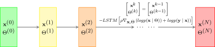
(a)

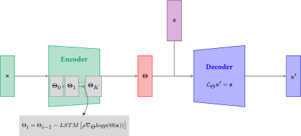
(b)

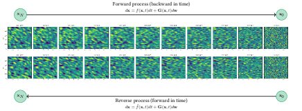
(c)

Figure 1: Example of analogies between our combination of SPDE prior and neural solver with generative models

In (4), we could consider using only the regularization cost if we are only interested to learn SPDE surrogate generative models using as training data gap-free states. In such a case, the proposed formulation relates to variational autoencoder (VAE) formulations (Kingma and Welling, 2022), see also Fig.1b), in which the encoder projects the state $\mathbf{x}$ to the parameter space $\Theta$. The encoder is trained on the NLL of $\Theta$. The decoder is simply the SPDE, and does not require any training. Back to the encoder part, it may compress the original high-dimensional input space into a lower-dimensional space, if the SPDE is stationary for instance. More generally, when complex spatio-temporal anisotropies are involved, and without a parametrization model for the latent variable $\Theta$, the latter has high dimensionality (same as the original data or higher), as it is done in diffusion-based models, see e.g. (Sohl-Dickstein et al., 2015; Ho et al., 2020). Along this line, starting from any initial conditions $\Theta_{0}$, the optimal set of parameters $\Theta^{\star}$ (given $\mathbf{x}$) would be obtained by the iterations:

$$\Theta_{i}=\Theta_{i+1}-\mathcal{K}\big{[}\rho\nabla_{\Theta}\mathrm{log}\ p(\mathbf{x}\mid\Theta)\big{]}$$

because the target cost function would not be the 4DVar cost anymore but its regularization part (prior cost), i.e. $\mathrm{log}\ p(\mathbf{x}\mid\Theta)$. As already said above, this relates to Langevin dynamics formalism.

Eq.(1) provides a simple way to generate SPDE-driven GP simulations starting from white or colored noise $\mathbf{z}_{0}$.It can be seen as the so-called reverse process in diffusion-based models (Ho et al., 2020). Because we deal with space-time processes, this reverse process would actually go forward in time, while the corresponding forward process would go backward in time till the initial noise used in the SPDE to generate realistic space-time sequences. Considering our formulation, the reverse process can be reformulated as follows:

$$\mathbf{x}_{i+1} =\mathbf{M}_{i+1}\mathbf{x}_{i}+\mathbf{T}_{i+1}\boldsymbol{z}_{i}$$

$$=\mathbf{x}_{i}-\mathbf{F}_{i+1}\mathbf{M}_{i+1}\mathbf{x}_{i}+\mathbf{T}_{i+1}\boldsymbol{z}_{i}$$ (22)

because of the Woodbury matrix identity $\mathbf{M}_{i+1}=\mathbf{I}-\mathbf{F}\mathbf{M}_{i+1}$. By (Anderson, 1982), we also know that given a forward process (data to noise):

$$\mathbf{x}_{i}=\mathbf{x}_{i+1}+\mathbf{f}_{i+1}(\mathbf{x}_{i+1})+\mathbf{G}_{i+1}\mathbf{z}_{i+1}$$

the corresponding reverse process (noise to data) writes:

$$\mathbf{x}_{i+1}=\mathbf{x}_{i}+\mathbf{f}_{i}(\mathbf{x}_{i}) -\frac{1}{2}\nabla\cdot\left[\mathbf{G}_{i}\mathbf{G}_{i}^{{\mathsf{T}}}\right]$$

$$-\frac{1}{2}\mathbf{G}_{i}\mathbf{G}_{i}^{{\mathsf{T}}}\nabla\mathrm{log}p_{i}(\mathbf{x}_{i})+\mathbf{G}_{i}\boldsymbol{z}_{i}$$

Then, by simple identification, the drift term $\mathbf{f}_{i}(\mathbf{x}_{i})$ is:

$$\mathbf{f}_{i}(\mathbf{x}_{i})=-\mathbf{F}_{i+1}\mathbf{M}_{i+1} +\frac{1}{2}\nabla\cdot\left[\mathbf{T}_{i+1}\mathbf{T}_{i}^{{\mathsf{T}}}\right]$$

$$+\frac{1}{2}\mathbf{T}_{i+1}\mathbf{T}_{i+1}^{{\mathsf{T}}}\mathbf{P}_{i+1}^{-1}\mathbf{x}_{i+1}$$ (23)

since $\nabla\mathrm{log}p_{i+1}(\mathbf{x}_{i+1})=-\mathbf{P}_{i+1}^{-1}\mathbf{x}_{i+1}$ Fig.1c) demonstrates this link when simulating with Eq. (4) a GP with global anisotropy on a uniform Cartesian grid with $dx$, $dy$ and $dt$ all set to one and shows how we can retrieve the forward process from Eq. (4). This opens a new challenge for future work to estimate the underlying stochastic differential equation of the forward process for space-time sequences, then being able to generate realistic space-time dynamics.

5 Experiments

We apply the proposed neural SPDE scheme to a real-world dataset, namely the interpolaton of sea surface height (SSH) fields from irregularly-sampled satellite altimetry observations Johnson et al. (2023). The SSH relates to sea surface dynamics (Le Guillou et al., 2020) and satellite altimetry data are characterized by an average missing data rate above 90%.

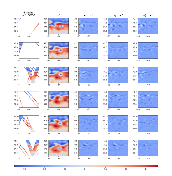
Figure 2: From left to right: Pseudo-observations (4 nadirs and SWOT), the reconstruction obtained with our neural SPDE variational solver, and deviations to the optimal reconstruction obtained from 3 conditional simulations. Results are given at the center of the data assimilation window along the 42 days test period and every 6 days (from top to bottom).

	$\mu$(RMSE)	$\sigma$(RMSE)	$\lambda_{x}$ (degree)	$\lambda_{t}$ (days)
OI (1 swot + 4 nadirs)	0.92	0.02	1.22	11.06
BFN	0.92	0.02	1.23	10.82
DYMOST	0.91	0.02	1.36	11.91
MIOST	0.93	0.01	1.35	10.41
UNet	0.92	0.02	1.25	11.33
UNet (time-dependent)	0.91	0.02	1.29	10.84
4DVarNet - UNet prior	0.94	0.01	1.17	6.86
4DVarNet - BilinRes prior	0.97	0.01	0.89	4.40
4DVarNet - SPDE prior	0.96	0.01	0.90	5.03

Table 1: Interpolation performance for the satellite altimetry case-study: for each benchmarked models, we report the considered performance metrics averaged on the test period.

Experimental setting

We exploit the experimental setting defined in (Johnson et al., 2023) . It relies on a groundtruthed dataset given by the simulation of realistic satellite altimetry observations from numerical ocean simulations. Overall, this dataset refers to 2d+t states for a $10^{\circ}\times 10^{\circ}$ domain with 1/20^∘ resolution corresponding to a small area in the Western part of the Gulf Stream. Regarding the evaluation framework, we refer the reader to SSH mapping data challenge above mentioned for a detailed presentation of the datasets and evaluation metrics. The latter comprise the MSE w.r.t the Ground Truth, the minimal spatial and temporal scales resolved. For learning-based approaches, the training dataset spans from mid-February 2013 to October 2013, while the validation period refers to January 2013. In all the reported experiments, we use Adam optimizer over 200 epochs and NVIDIA A100 Tensor Core mono-GPU architectures. All methods are tested on the test period from October 22, 2012 to December 2, 2012.

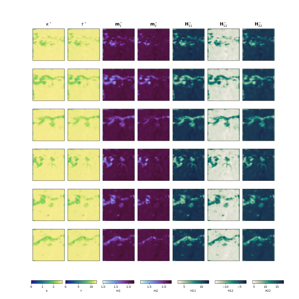
Figure 3: Parameter estimation of the SPDE prior in the neural scheme along the 42 days test period and every 6 days. From left to right: dumpin and variance parameters, advection fields and diffusion tensors.

Benchmarked models

For benchmarking purposes, we consider the approaches reported in Le Guillou et al. (2020), namely: the operational baseline (DUACS) based on an optimal interpolation, multi-scale OI scheme MIOST (Ardhuin et al., 2020) and model-driven interpolation schems BFN (Le Guillou et al., 2020) and DYMOST (Ubelmann et al., 2016; Ballarotta et al., 2020). We also include a state-of-the-art UNet architecture to train a direct inversion scheme Cicek et al. (2016). As stated in Section 4, we also implemented a time-dependent UNet to approximate the gradient of the log-prior distribution $\nabla\mathrm{log}p({\mathbf{x}})$ to replace our LSTM solver. Last, for all neural schemes, we consider $N=$ 15 days space-time sequences to account for time scales considered in state-of-the-art OI schemes. Regarding the parameterization of our framework, we consider a bilinear residual architecture for prior $\Phi$, the same UNet used in the direct inversion and the SPDE prior proposed throughout the paper. For the solver $\Gamma$, we use a 2d convolutional LSTM cell with 150-dimensional hidden states.

Results

Table 1 further highlights the performance gain of the proposed scheme. The relative gain is greater than 50% compared to the operational satellite altimetry processing. We outperform by more than 20% in terms of relative gain to the baseline MIOST and UNet schemes, which are the second best interpolation schemes. Interestingly, our scheme is the only one to retrieve time scales below 10 days. Figure 2 displays the reconstruction obtained with our neural variational scheme as well as the deviations to the optimal reconstruction obtained from 3 conditional simulations, see Eq. (20): we can see how their variance is high along the main meander of the Gulf Stream and highly energetic eddies but lower elsewhere. Regarding Figure 3 and the SPDE parameters estimated along the 42 days test period every 6 days, they seem consistent with state $\mathbf{x}$ that partially encodes the SPDE parametrization. The capability of our approach to span parameter distribution that are not standardized is demonstrated, which is particularly the case for the diffusion tensor $\mathbf{H}$. Last, Figure 4 shows the posterior standard deviations computed when using the SPDE-based generation of 250 members and the reconstruction error $\mathbf{x}-\mathbf{x}^{\star}$ for the tenth day of the test period. Contrary to OI, the posterior variance is not only conditioned by the observations, it is more continuous and flow dependent. The correlation with the reconstruction error is good, thus it is consistent: when low, the average reconstruction is generally very good.

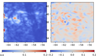
Figure 4: Ensemble-based posterior standard deviations and reconstruction error $\mathbf{x}-\mathbf{x}^{\star}$

6 Conclusion

We have derived a new neural architecture to tackle the reconstruction of a dynamical process from partial and noisy observations. Both state trajectory and stochastic prior parametrization are learnt so that we also provide uncertainty quantification of the mean state. In this work, we use an SPDE-driven GP as flexible prior whose parameters are added as latent variables in an augmented state. A bi-level optimization scheme is used on both the inner variational cost derived from OI-based formulations and the outer training loss function of the neural architecture, which drives the optimization of the LSTM-based residual solver leading to the reconstruction of the state.

Checklist

1. For all models and algorithms presented, check if you include:

   1. A clear description of the mathematical setting, assumptions, algorithm, and/or model. [Yes/No/Not Applicable]. Yes, more specifically in Sections 2 and 3

   2. An analysis of the properties and complexity (time, space, sample size) of any algorithm. [Yes/No/Not Applicable] Yes, when useful, e.g. complexity of OI with sparse precision matrices

   3. (Optional) Anonymized source code, with specification of all dependencies, including external libraries. [Yes/No/Not Applicable] Yes, the GitHub repository will be provided in the final version of the paper

2. For any theoretical claim, check if you include:

   1. Statements of the full set of assumptions of all theoretical results. [Yes/No/Not Applicable] Yes, see Section 2 on the SPDE formulation of the prior

   2. Complete proofs of all theoretical results. [Yes/No/Not Applicable] Yes, see the Supplementary materials

   3. Clear explanations of any assumptions. [Yes/No/Not Applicable] Yes, Sections 2 and 3

3. For all figures and tables that present empirical results, check if you include:

   1. The code, data, and instructions needed to reproduce the main experimental results (either in the supplemental material or as a URL). [Yes/No/Not Applicable] Yes, the GitHub repository will be provided in the final version of the paper. As outputs of the main code, a NetCDF file is produced, the same used to fill in the Table and produce the figures

   2. All the training details (e.g., data splits, hyperparameters, how they were chosen). [Yes/No/Not Applicable] Yes, see Section 5: experimental settings

   3. A clear definition of the specific measure or statistics and error bars (e.g., with respect to the random seed after running experiments multiple times). [Yes/No/Not Applicable] [Yes/No/Not Applicable] Yes, in Section 5 we provide the reference of the data challenge where the main metrics are precisely defined

   4. A description of the computing infrastructure used. (e.g., type of GPUs, internal cluster, or cloud provider). [Yes/No/Not Applicable] Yes, see Section 5: experimental settings

4. If you are using existing assets (e.g., code, data, models) or curating/releasing new assets, check if you include:

   1. Citations of the creator If your work uses existing assets. [Yes/No/Not Applicable] Yes, see Section 5 in which we provide the url of the data challenge related to our experiment

   2. The license information of the assets, if applicable. [Yes/No/Not Applicable] Not applicable

   3. New assets either in the supplemental material or as a URL, if applicable. [Yes/No/Not Applicable] Yes, the GitHub repository will be provided in the final version of the paper.

   4. Information about consent from data providers/curators. [Yes/No/Not Applicable] Not applicable

   5. Discussion of sensible content if applicable, e.g., personally identifiable information or offensive content. [Yes/No/Not Applicable] Not applicable

5. If you used crowdsourcing or conducted research with human subjects, check if you include:

   1. The full text of instructions given to participants and screenshots. [Yes/No/Not Applicable] Not applicable

   2. Descriptions of potential participant risks, with links to Institutional Review Board (IRB) approvals if applicable. [Yes/No/Not Applicable] Not applicable

   3. The estimated hourly wage paid to participants and the total amount spent on participant compensation. [Yes/No/Not Applicable] Not applicable

References

- Aggarwal et al. [2019] H. K. Aggarwal, M. P. Mani, and M. Jacob. MoDL: Model-Based Deep Learning Architecture for Inverse Problems. IEEE Transactions on Medical Imaging, 38(2):394–405, Feb. 2019. ISSN 1558-254X. doi: 10.1109/TMI.2018.2865356. Conference Name: IEEE Transactions on Medical Imaging.
- Anderson [1982] B. D. Anderson. Reverse-time diffusion equation models. Stochastic Processes and their Applications, 12(3):313–326, May 1982. URL https://ideas.repec.org/a/eee/spapps/v12y1982i3p313-326.html.
- Andrychowicz et al. [2016] M. Andrychowicz, M. Denil, S. Gomez, M. W. Hoffman, D. Pfau, T. Schaul, B. Shillingford, and N. De Freitas. Learning to learn by gradient descent by gradient descent. In Advances in neural information processing systems, pages 3981–3989, 2016.
- Ardhuin et al. [2020] F. Ardhuin, C. Ubelmann, G. Dibarboure, L. Gaultier, A. Ponte, M. Ballarotta, and Y. Faugère. Reconstructing ocean surface current combining altimetry and future spaceborne doppler data. Earth and Space Science Open Archive, page 22, 2020. doi: 10.1002/essoar.10505014.1. URL https://doi.org/10.1002/essoar.10505014.1.
- Asch et al. [2016] M. Asch, M. Bocquet, and M. Nodet. Data Assimilation. Fundamentals of Algorithms. Society for Industrial and Applied Mathematics, Dec. 2016. ISBN 978-1-61197-453-9. doi: 10.1137/1.9781611974546. URL https://doi.org/10.1137/1.9781611974546.
- Aubert and Kornprobst [2006] G. Aubert and P. Kornprobst. Mathematical problems in image processing: partial differential equations and the calculus of variations, volume 147. Springer Science & Business Media, 2006. ISBN 0-387-44588-9.
- Aune et al. [2013] E. Aune, J. Eidsvik, and Y. Pokern. Iterative numerical methods for sampling from high dimensional gaussian distributions. Statistics and Computing, 23(4):501–521, Jul 2013. ISSN 1573-1375. doi: 10.1007/s11222-012-9326-8. URL https://doi.org/10.1007/s11222-012-9326-8.
- Ballarotta et al. [2020] M. Ballarotta, C. Ubelmann, M. Rogé, F. Fournier, Y. Faugère, G. Dibarboure, R. Morrow, and N. Picot. Dynamic mapping of along-track ocean altimetry: Performance from real observations. Journal of Atmospheric and Oceanic Technology, 37(9):1593 – 1601, 2020. doi: 10.1175/JTECH-D-20-0030.1. URL https://journals.ametsoc.org/view/journals/atot/37/9/jtechD200030.xml.
- Beauchamp et al. [2023a] M. Beauchamp, Q. Febvre, H. Georgenthum, and R. Fablet. 4dvarnet-ssh: end-to-end learning of variational interpolation schemes for nadir and wide-swath satellite altimetry. Geoscientific Model Development, 16(8):2119–2147, 2023a. doi: 10.5194/gmd-16-2119-2023. URL https://gmd.copernicus.org/articles/16/2119/2023/.
- Beauchamp et al. [2023b] M. Beauchamp, Q. Febvre, J. Thompson, H. Georgenthum, and R. Fablet. Learning neural optimal interpolation models and solvers. In J. Mikyška, C. de Mulatier, M. Paszynski, V. V. Krzhizhanovskaya, J. J. Dongarra, and P. M. Sloot, editors, Computational Science – ICCS 2023, pages 367–381, Cham, 2023b. Springer Nature Switzerland. ISBN 978-3-031-36027-5.
- Bertalmio et al. [2001] M. Bertalmio, A. L. Bertozzi, and G. Sapiro. Navier-Stokes, fluid dynamics, and image and video inpainting. In IEEE CVPR, pages 355–362, 2001.
- Bolin and Wallin [2016] D. Bolin and J. Wallin. Spatially adaptive covariance tapering. Spatial Statistics, 18:163–178, 2016. ISSN 2211-6753. doi: https://doi.org/10.1016/j.spasta.2016.03.003. URL https://www.sciencedirect.com/science/article/pii/S2211675316000245. Spatial Statistics Avignon: Emerging Patterns.
- Boudier et al. [2023] P. Boudier, A. Fillion, S. Gratton, S. Gürol, and S. Zhang. Data assimilation networks. Journal of Advances in Modeling Earth Systems, 15(4):e2022MS003353, 2023. doi: https://doi.org/10.1029/2022MS003353. URL https://agupubs.onlinelibrary.wiley.com/doi/abs/10.1029/2022MS003353. e2022MS003353 2022MS003353.
- Carrizo Vergara [2018] R. Carrizo Vergara. Development of geostatistical models using Stochastic Partial Differential Equations. Theses, Mines ParisTech - PSL University, Dec. 2018. URL https://hal.archives-ouvertes.fr/tel-02126057.
- Charlier et al. [2020] B. Charlier, J. Feydy, J. A. Glaunès, F.-D. Collin, and G. Durif. Kernel operations on the gpu, with autodiff, without memory overflows. 2020. doi: 10.48550/ARXIV.2004.11127. URL https://arxiv.org/abs/2004.11127.
- Chilès and Delfiner [2012] J. Chilès and P. Delfiner. Geostatistics : modeling spatial uncertainty. Wiley, New-York, second edition, 2012.
- Chilès and Desassis [2018] J.-P. Chilès and N. Desassis. Fifty Years of Kriging, pages 589–612. Springer International Publishing, Cham, 2018. ISBN 978-3-319-78999-6. doi: 10.1007/978-3-319-78999-6“˙29. URL https://doi.org/10.1007/978-3-319-78999-6\_29.
- Cicek et al. [2016] O. Cicek, A. Abdulkadir, S. Lienkamp, T. Brox, and O. Ronneberger. 3D U-Net: learning dense volumetric segmentation from sparse annotation. In Proc. MICCAI, pages 424–432, 2016.
- Clarotto et al. [2022] L. Clarotto, D. Allard, T. Romary, and N. Desassis. The spde approach for spatio-temporal datasets with advection and diffusion, 2022. URL https://arxiv.org/abs/2208.14015.
- Cressie and Wikle [2015] N. Cressie and C. Wikle. Statistics for Spatio-Temporal Data. John Wiley & Sons, 2015. ISBN 978-1-119-24304-5.
- Cutajar et al. [2016] K. Cutajar, M. Osborne, J. Cunningham, and M. Filippone. Preconditioning kernel matrices. In IEEE, editor, ICML 2016, International Conference on Machine Learning, June 19-24, 2016, San Francisco, USA, San Francisco, 2016. © 2016 IEEE. Personal use of this material is permitted. However, permission to reprint/republish this material for advertising or promotional purposes or for creating new collective works for resale or redistribution to servers or lists, or to reuse any copyrighted component of this work in other works must be obtained from the IEEE.
- Dinh et al. [2017] L. Dinh, J. Sohl-Dickstein, and S. Bengio. Density estimation using real nvp, 2017.
- Evensen [2009] G. Evensen. Data Assimilation. Springer Berlin Heidelberg, Berlin, Heidelberg, 2009. ISBN 9783642037108 9783642037115. URL http://link.springer.com/10.1007/978-3-642-03711-5.
- Evensen et al. [2022] G. Evensen, , F. C. Vossepoel, and P. J. van Leeuwen. Data Assimilation Fundamentals. Springer Textbooks in Earth Sciences, Geography and Environment (STEGE). Springer Cham, 2022. ISBN 978-3-030-96708-6. doi: 10.1007/978-3-030-96709-3. URL https://doi.org/10.1007/978-3-030-96709-3.
- Fablet et al. [2020] R. Fablet, L. Drumetz, and F. Rousseau. Joint learning of variational representations and solvers for inverse problems with partially-observed data. arXiv:2006.03653 [physics], 2020. URL https://arxiv.org/abs/2006.03653. arXiv:2006.03653.
- Fuglstad et al. [2015a] G.-A. Fuglstad, F. Lindgren, D. Simpson, and H. Rue. Exploring a new class of non-stationary spatial gaussian random fields with varying local anisotropy. Statistica Sinica, 25(1):115–133, 2015a. ISSN 1017-0405. doi: 10.5705/ss.2013.106w.
- Fuglstad et al. [2015b] G.-A. Fuglstad, D. Simpson, F. Lindgren, and H. Rue. Does non-stationary spatial data always require non-stationary random fields? Spatial Statistics, 14:505–531, 2015b. ISSN 2211-6753. doi: https://doi.org/10.1016/j.spasta.2015.10.001. URL https://www.sciencedirect.com/science/article/pii/S2211675315000780.
- Fuglstad et al. [2015c] G.-A. Fuglstad, D. Simpson, F. Lindgren, and H. Rue. Does non-stationary spatial data always require non-stationary random fields? Spatial Statistics, 14:505 – 531, 2015c. ISSN 2211-6753. doi: https://doi.org/10.1016/j.spasta.2015.10.001. URL http://www.sciencedirect.com/science/article/pii/S2211675315000780.
- Furrer et al. [2006] R. Furrer, M. G. Genton, and D. Nychka. Covariance tapering for interpolation of large spatial datasets. Journal of Computational and Graphical Statistics, 15(3):502–523, 2006. ISSN 10618600. URL http://www.jstor.org/stable/27594195.
- Goodfellow et al. [2014] I. J. Goodfellow, J. Pouget-Abadie, M. Mirza, B. Xu, D. Warde-Farley, S. Ozair, A. Courville, and Y. Bengio. Generative adversarial nets. In Proceedings of the 27th International Conference on Neural Information Processing Systems - Volume 2, NIPS’14, page 2672–2680, Cambridge, MA, USA, 2014. MIT Press.
- Grenander and Miller [1994] U. Grenander and M. I. Miller. Representations of knowledge in complex systems. Journal of the Royal Statistical Society. Series B (Methodological), 56(4):549–603, 1994. ISSN 00359246. URL http://www.jstor.org/stable/2346184.
- Ho et al. [2020] J. Ho, A. Jain, and P. Abbeel. Denoising diffusion probabilistic models, 2020.
- Johnson et al. [2023] J. E. Johnson, Q. Febvre, A. Gorbunova, S. Metref, M. Ballarotta, J. L. Sommer, and R. Fablet. Oceanbench: The sea surface height edition, 2023.
- Kingma and Welling [2022] D. P. Kingma and M. Welling. Auto-encoding variational bayes, 2022.
- Le Guillou et al. [2020] F. Le Guillou, S. Metref, E. Cosme, C. Ubelmann, M. Ballarotta, J. Verron, and J. Le Sommer. Mapping altimetry in the forthcoming swot era by back-and-forth nudging a one-layer quasi-geostrophic model. Earth and Space Science Open Archive, page 15, 2020. doi: 10.1002/essoar.10504575.1. URL https://doi.org/10.1002/essoar.10504575.1.
- Lindgren et al. [2011] F. Lindgren, H. Rue, and J. Lindström. An explicit link between gaussian fields and gaussian markov random fields: the stochastic partial differential equation approach. Journal of the Royal Statistical Society: Series B (Statistical Methodology), 73(4):423–498, 2011. doi: 10.1111/j.1467-9868.2011.00777.x. URL https://rss.onlinelibrary.wiley.com/doi/abs/10.1111/j.1467-9868.2011.00777.x.
- Lucas et al. [2018] A. Lucas, M. Iliadis, R. Molina, and A. Katsaggelos. Using Deep Neural Networks for Inverse Problems in Imaging: Beyond Analytical Methods. IEEE SPM, 35(1):20–36, 2018. ISSN 1558-0792. doi: 10.1109/MSP.2017.2760358.
- McCann et al. [2017] M. McCann, K. Jin, and M. Unser. Convolutional Neural Networks for Inverse Problems in Imaging: A Review. IEEE SPM, 34(6):85–95, 2017. ISSN 1558-0792. doi: 10.1109/MSP.2017.2739299.
- Nocedal and Wright [2006] J. Nocedal and S. J. Wright. Numerical Optimization. Springer, New York, NY, USA, 2e edition, 2006.
- Pereira and Desassis [2019] M. Pereira and N. Desassis. Efficient simulation of Gaussian Markov random fields by Chebyshev polynomial approximation. Spatial Statistics, 31:100359, June 2019. doi: 10.1016/j.spasta.2019.100359. URL https://hal.science/hal-02283801.
- Pereira et al. [2022] M. Pereira, N. Desassis, and D. Allard. Geostatistics for large datasets on riemannian manifolds: A matrix-free approach. Journal of Data Science, 20(4):512–532, 2022. ISSN 1680-743X. doi: 10.6339/22-JDS1075.
- Pleiss et al. [2020] G. Pleiss, M. Jankowiak, D. Eriksson, A. Damle, and J. R. Gardner. Fast matrix square roots with applications to gaussian processes and bayesian optimization, 2020. URL https://arxiv.org/abs/2006.11267.
- Powell [2011] P. D. Powell. Calculating determinants of block matrices, 2011.
- Romary and Desassis [2018] T. Romary and N. Desassis. Combining covariance tapering and lasso driven low rank decomposition for the kriging of large spatial datasets, 2018. URL https://arxiv.org/abs/1806.01558.
- Rue et al. [2017] H. Rue, A. Riebler, S. H. Sørbye, J. B. Illian, D. P. Simpson, and F. K. Lindgren. Bayesian computing with inla: A review. Annual Review of Statistics and Its Application, 4(1):395–421, 2017. doi: 10.1146/annurev-statistics-060116-054045. URL https://doi.org/10.1146/annurev-statistics-060116-054045.
- Saad [2003] Y. Saad. Iterative Methods for Sparse Linear Systems. Society for Industrial and Applied Mathematics, second edition, 2003. doi: 10.1137/1.9780898718003. URL https://epubs.siam.org/doi/abs/10.1137/1.9780898718003.
- Särkkä and Solin [2019] S. Särkkä and A. Solin. Applied Stochastic Differential Equations. Institute of Mathematical Statistics Textbooks. Cambridge University Press, 2019. doi: 10.1017/9781108186735.
- Shi et al. [2015] X. Shi, Z. Chen, H. Wang, D.-Y. Yeung, W.-K. Wong, and W.-C. Woo. Convolutional lstm network: A machine learning approach for precipitation nowcasting. In C. Cortes, N. Lawrence, D. Lee, M. Sugiyama, and R. Garnett, editors, Advances in Neural Information Processing Systems, volume 28. Curran Associates, Inc., 2015. URL https://proceedings.neurips.cc/paper/2015/file/07563a3fe3bbe7e3ba84431ad9d055af-Paper.pdf.
- Sigrist et al. [2015] F. Sigrist, H. R. Künsch, and W. A. Stahel. Stochastic partial differential equation based modelling of large space–time data sets. Journal of the Royal Statistical Society: Series B (Statistical Methodology), 77(1):3–33, 2015. doi: https://doi.org/10.1111/rssb.12061. URL https://rss.onlinelibrary.wiley.com/doi/abs/10.1111/rssb.12061.
- Sohl-Dickstein et al. [2015] J. Sohl-Dickstein, E. A. Weiss, N. Maheswaranathan, and S. Ganguli. Deep unsupervised learning using nonequilibrium thermodynamics, 2015.
- Tandeo et al. [2020] P. Tandeo, P. Ailliot, M. Bocquet, A. Carrassi, T. Miyoshi, M. Pulido, and Y. Zhen. A review of innovation-based methods to jointly estimate model and observation error covariance matrices in ensemble data assimilation. Monthly Weather Review, 148(10):3973–3994, Oct 2020. ISSN 1520-0493. doi: 10.1175/mwr-d-19-0240.1. URL http://dx.doi.org/10.1175/MWR-D-19-0240.1.
- Traon et al. [1998] P.-Y. Traon, F. Nadal, and N. Ducet. An improved mapping method of multisatellite altimeter data. Journal of Atmospheric and Oceanic Technology, 15(2):522–534, 1998. doi: 10.1175/1520-0426(1998)015¡0522:AIMMOM¿2.0.CO;2. URL https://journals.ametsoc.org/view/journals/atot/15/2/1520-0426\_1998\_015\_0522\_aimmom\_2\_0\_co\_2.xml.
- Ubelmann et al. [2016] C. Ubelmann, B. Cornuelle, and L.-L. Fu. Dynamic mapping of along-track ocean altimetry: Method and performance from observing system simulation experiments. Journal of Atmospheric and Oceanic Technology, 33(8):1691 – 1699, 2016. doi: 10.1175/JTECH-D-15-0163.1. URL https://journals.ametsoc.org/view/journals/atot/33/8/jtech-d-15-0163_1.xml.
- Wackernagel [2003] H. Wackernagel. Multivariate Geostatistics. An Introduction with Applications. Springer-Verlag Berlin Heidelberg, New York, 2003. doi: 10.1007/978-3-662-05294-5. ISBN 978-3-540-44142-7.
- Whittle [1953] P. Whittle. On stationary processes in the plane. Biometrika, 41(3-4):434–449, 1953. doi: 10.1093/biomet/41.3-4.434. URL http://biomet.oxfordjournals.org/content/41/3-4/434.short.