Solving Kernel Ridge Regression with Gradient Descent for a Non-Constant Kernel

Abstract

Kernel ridge regression, KRR, is a generalization of linear ridge regression that is non-linear in the data, but linear in the parameters. The solution can be obtained either as a closed-form solution, which includes a matrix inversion, or iteratively through gradient descent. Using the iterative approach opens up for changing the kernel during training, something that is investigated in this paper. We theoretically address the effects this has on model complexity and generalization. Based on our findings, we propose an update scheme for the bandwidth of translational-invariant kernels, where we let the bandwidth decrease to zero during training, thus circumventing the need for hyper-parameter selection. We demonstrate on real and synthetic data how decreasing the bandwidth during training outperforms using a constant bandwidth, selected by cross-validation and marginal likelihood maximization. We also show theoretically and empirically that using a decreasing bandwidth, we are able to achieve both zero training error in combination with good generalization, and a double descent behavior, phenomena that do not occur for KRR with constant bandwidth but are known to appear for neural networks.

Keywords: Kernel Ridge Regression, Gradient Descent, Gradient Flow, Hyper-Parameter Selection, Double Descent

1 Introduction

Kernel ridge regression, KRR, is a generalization of linear ridge regression that is non-linear in the data, but linear in the parameters. Just as for linear ridge regression, KRR has a closed-form solution, however at the cost of inverting an $n\times n$ matrix, where $n$ is the number of training observations. The KRR estimate coincides with the posterior mean of kriging, or Gaussian process regression, (Krige,, 1951; Matheron,, 1963) and has successfully been applied within a wide range of applications (Zahrt et al.,, 2019; Ali et al.,, 2020; Chen and Leclair,, 2021; Fan et al.,, 2021; Le et al.,, 2021; Safari and Rahimzadeh Arashloo,, 2021; Shahsavar et al.,, 2021; Singh Alvarado et al.,, 2021; Wu et al.,, 2021; Chen et al.,, 2022).

Solving kernel regression with gradient descent, something we refer to as kernel gradient descent, KGD, but which is also known as functional gradient descent (Mason et al.,, 1999), has been studied by e.g. Yao et al., (2007), Raskutti et al., (2014), Ma and Belkin, (2017), and Allerbo, (2023). The algorithm requires $\mathcal{O}(Tn^{2})$ operations, where $T$ is the number of iterations and $n$ is the number of observations, which is more computationally efficient than the $\mathcal{O}(n^{3})$ operations of the matrix inversion step in the closed-form solution for problems where $T$ is smaller than $n$.

In addition to computational efficiency, the theoretical understandings from solving simpler regression problems, such as kernel regression, using gradient-based methods can be used for a deeper understanding of more complex regression models, such as neural networks (Belkin et al.,, 2018; Bartlett et al.,, 2021). Perhaps counter-intuitively, overparameterized neural networks, where the number of parameters is larger than the number of observations, tend to generalize well (Zhang et al.,, 2021), a phenomenon often referred to as double descent (Advani et al.,, 2020; Belkin et al.,, 2019). Jacot et al., (2018) showed that for highly overparameterized neural networks, the model updates are virtually linear in the parameters, with perfect linearity when the number of parameters goes to infinity. That is, the network is linear in the parameters, but non-linear in the data, just as kernel regression. In fact, a neural network that is linear in its parameters can equivalently be expressed as kernel regression, with a kernel that is a function of the network architecture and the parameter values at initialization. The authors refer to this kernel as the neural tangent kernel. Training a (highly) overparameterized neural network with gradient descent is thus (basically) equivalent to solving kernel regression with gradient descent.

Both the neural tangent kernel interpretation, and the solutions of KGD, assume that the kernel is constant during training. However, for neural networks with finitely many parameters, this is not the case. Furthermore, the model complexity of neural networks is known to increase with training (Kalimeris et al.,, 2019). Thus, training a neural network can be thought of as KGD with a kernel whose complexity increases during training.

In this paper, we introduce kernel gradient descent with a non-constant kernel, whose complexity increases during training. In Section 2, we review KRR, KGD, and kernel gradient flow, KGF, which is how we refer to KGD with infinitesimal step size. In Section 3, we analyze KGD for non-constant kernels in terms of generalization and model complexity. Based on these analyses, we propose an update scheme for the bandwidth of translational-invariant kernels. In Section 4, we theoretically analyze the double descent phenomenon for KGD with non-constant bandwidth. In Section 5, we empirically verify our theoretical results on real and synthetic data.

Our main contributions are listed below.

• We analyze the generalization properties of KGD with a non-constant kernel.

• For translational-invariant kernels we

  • present a theoretically justified kernel update scheme for the bandwidth.

  • theoretically analyze the occurrence of double descent.

• For several different translational-invariant kernels, we demonstrate, on real and synthetic data, that compared to a constant bandwidth, a non-constant bandwidth leads to

  • a better model performance.

  • zero training error in combination with good generalization.

  • a double descent behavior.

All proofs are deferred to Appendix A.

2 Review of Kernel Ridge Regression, Kernel Gradient Descent and Kernel Gradient Flow

For a positive semi-definite kernel function, $k(\bm{x},\bm{x^{\prime}})\in\mathbb{R}$, and $n$ paired observations, $(\bm{x_{i}},y_{i})_{i=1}^{n}\in\mathbb{R}^{p}\times\mathbb{R}$, presented in a design matrix, $\bm{X}=[\bm{x_{1}}^{\top},\bm{x_{2}}^{\top},\dots\bm{x_{n}}^{\top}]^{\top}\in\mathbb{R}^{n\times p}$, and a response vector, $\bm{y}\in\mathbb{R}^{n}$, and for a given regularization strength, $\lambda>0$, the objective function of kernel ridge regression, KRR, is given by

$$\bm{\hat{\alpha}}=\operatorname*{arg\,min}_{\bm{\alpha}\in\mathbb{R}^{n}}\frac{1}{2}\left\|\bm{y}-\bm{K}\bm{\alpha}\right\|_{2}^{2}+\frac{\lambda}{2}\|\bm{\alpha}\|^{2}_{\bm{K}}=\left(\bm{K}+\lambda\bm{I}\right)^{-1}\bm{y},$$ (1)

$$\begin{bmatrix}\bm{\hat{f}}\\ \bm{\hat{f}^{*}}\end{bmatrix}=\begin{bmatrix}\bm{K}\\ \bm{K^{*}}\end{bmatrix}\bm{\hat{\alpha}}=\begin{bmatrix}\bm{K}\\ \bm{K^{*}}\end{bmatrix}\left(\bm{K}+\lambda\bm{I}\right)^{-1}\bm{y}.$$

Here, the two kernel matrices $\bm{K}=\bm{K}(\bm{X},\bm{X})\in\mathbb{R}^{n\times n}$ and $\bm{K^{*}}=\bm{K^{*}}(\bm{X^{*}},\bm{X})\in\mathbb{R}^{n^{*}\times n}$ are defined according to $\bm{K}_{ij}=k(\bm{x_{i}},\bm{x_{j}})$ and $\bm{K^{*}}_{ij}=k(\bm{x^{*}_{i}},\bm{x_{j}})$, where $\bm{X^{*}}=[\bm{x^{*}_{1}}{{}^{\top}},\bm{x^{*}_{2}}{{}^{\top}},\dots\bm{x^{*}_{n^{*}}}{{}^{\top}}]^{\top}\in\mathbb{R}^{n^{*}\times p}$ denotes new data. The vectors $\bm{\hat{f}}=\bm{\hat{f}}(\bm{X})=[\hat{f}(\bm{x_{1}}),\hat{f}(\bm{x_{2}}),\dots\hat{f}(\bm{x_{n}})]^{\top}\in\mathbb{R}^{n}$ and $\bm{\hat{f}^{*}}=\bm{\hat{f}^{*}}(\bm{X^{*}},\bm{X})=[\hat{f}(\bm{x^{*}_{1}}),\hat{f}(\bm{x^{*}_{2}}),\dots\hat{f}(\bm{x^{*}_{n^{*}}})]^{\top}\in\mathbb{R}^{n^{*}}$ denote model predictions on training and new data, respectively. For a single prediction, $\hat{f}(\bm{x^{*}})\in\bm{\hat{f}^{*}}$, $\hat{f}(\bm{x^{*}})=\hat{f}(\bm{x^{*}},\lambda)={\bm{k^{*}}}^{\top}(\bm{K}+\lambda\bm{I})^{-1}\bm{y}$, where ${\bm{k^{*}}}^{\top}=\bm{k^{*}}(\bm{x^{*}},\bm{X})^{\top}\in\mathbb{R}^{n}$ is the corresponding row in $\bm{K^{*}}$. The weighted norm, $\|\bm{v}\|_{\bm{A}}$, is defined according to $\|\bm{v}\|_{\bm{A}}^{2}=\bm{v}^{\top}\bm{A}\bm{v}$ for any symmetric positive definite matrix $\bm{A}$.

The similarities between ridge regression and gradient descent with early stopping are well studied for linear regression (Friedman and Popescu,, 2004; Ali et al.,, 2019; Allerbo et al.,, 2023). In the context of early stopping, optimization time can be thought of as an inverse penalty, where longer optimization time corresponds to weaker regularization. For gradient descent with infinitesimal step size, often referred to as gradient flow, a closed-form solution exists which allows for direct comparisons to ridge regression. The generalization of gradient flow from the linear to the kernel setting was studied by Allerbo, (2023), who used the names kernel gradient descent, KGD, and kernel gradient flow, KGF. Sometimes, the name functional gradient descent is used rather than KGD.

The update rule for KGD, with step size $\eta$, is given by

$$\begin{bmatrix}\bm{\hat{f}}_{k+1}\\ \bm{\hat{f}^{*}}_{k+1}\end{bmatrix}=\begin{bmatrix}\bm{\hat{f}}_{k}\\ \bm{\hat{f}^{*}}_{k}\end{bmatrix}+\eta\cdot\begin{bmatrix}\bm{K}\\ \bm{K^{*}}\end{bmatrix}\left(\bm{y}-\bm{\hat{f}}_{k}\right),\ \begin{bmatrix}\bm{\hat{f}}_{0}\\ \bm{\hat{f}^{*}}_{0}\end{bmatrix}=\begin{bmatrix}\bm{\mu}\\ \bm{\mu^{*}}\end{bmatrix},$$ (2)

where $[\bm{\mu}^{\top},\ {\bm{\mu^{*}}}^{\top}]^{\top}=[\bm{\mu}(\bm{X})^{\top},\ \bm{\mu^{*}}(\bm{X^{*}})^{\top}]^{\top}$ for some prior function $\mu(\bm{x})$.

The KGF solution is obtained by treating Equation 2 as the Euler forward formulation of the differential equation in Equation 3,

$$\frac{\partial}{\partial t}\left(\begin{bmatrix}\bm{\hat{f}}(t)\\ \bm{\hat{f}^{*}}(t)\end{bmatrix}\right)=\begin{bmatrix}\bm{K}\\ \bm{K^{*}}\end{bmatrix}\left(\bm{y}-\bm{\hat{f}}(t)\right),\ \begin{bmatrix}\bm{\hat{f}}(0)\\ \bm{\hat{f}^{*}}(0)\end{bmatrix}=\begin{bmatrix}\bm{\mu}\\ \bm{\mu^{*}}\end{bmatrix},$$ (3)

whose solution is given by

$$\begin{bmatrix}\bm{\hat{f}}(t)\\ \bm{\hat{f}^{*}}(t)\end{bmatrix}=\begin{bmatrix}\bm{I}\\ \bm{K^{*}}\bm{K}^{-1}\end{bmatrix}(\bm{I}-\exp(-t\bm{K}))(\bm{y}-\bm{\mu})+\begin{bmatrix}\bm{\mu}\\ \bm{\mu^{*}}\end{bmatrix},$$ (4)

where $\exp$ denotes the matrix exponential.
Remark 1: Note that $\bm{K}^{-1}(\bm{I}-\exp(-t\bm{K}))\bm{K}^{-1}=(\bm{I}-\exp(-t\bm{K}))\bm{K}^{-1}$ is well-defined even when $\bm{K}$ is singular. The matrix exponential is defined through its Taylor approximation and from $\bm{I}-\exp(-t\bm{K})=t\bm{K}-\frac{1}{2!}t^{2}\bm{K}^{2}+\dots$, a matrix $\bm{K}$ factors out, that cancels with $\bm{K}^{-1}$.
Remark 2: For KGD, the prior function, $\mu(\bm{x})$, is trivially incorporated as the initialization vector $[\bm{\mu}^{\top},\ {\bm{\mu^{*}}}^{\top}]^{\top}$. For KRR, the prior function can be included by shifting both $\bm{y}$ and $f$ with it, i.e. by replacing $\bm{y}$ and $[\bm{\hat{f}}^{\top},\ \bm{\hat{f}^{*}}\,^{\top}]^{\top}$ by $\bm{y_{\mu}}:=\bm{y}-\bm{\mu}$ and $[\bm{\hat{f}_{\mu}}^{\top},\ \bm{\hat{f}^{*}_{\mu}}\,^{\top}]^{\top}:=[(\bm{\hat{f}}-\bm{\mu})^{\top},\ (\bm{\hat{f}^{*}}-\bm{\mu^{*}})^{\top}]^{\top}$ in Equation 1. To alleviate notation, we henceforth use the prior shifted observations and predictions also for KGF, rewriting Equation 4 as

$$\begin{bmatrix}\bm{\hat{f}_{\mu}}(t)\\ \bm{\hat{f}^{*}_{\mu}}(t)\end{bmatrix}=\begin{bmatrix}\bm{I}\\ \bm{K^{*}}\bm{K}^{-1}\end{bmatrix}(\bm{I}-\exp(-t\bm{K}))\bm{y_{\mu}}.$$ (5)

3 Kernel Gradient Descent with Non-Constant Kernels

If we allow $[\bm{K}^{\top}\,{\bm{K^{*}}}^{\top}]^{\top}$ to vary between time steps in Equation 2, we obtain KGD with non-constant kernels. Below, we theoretically analyze the effects of this, discuss the implications for generalization, and propose an algorithm for kernel update during training.

We base our analysis of generalization on the axiom that for generalization to be good, the inferred function should deviate roughly as much from the prior function as the training data does. That is, if the training data follows the prior closely, so should the inferred function, and if the training data deviates from the prior, so should the inferred function.

Axiom 1.

For generalization to be good, the deviation between the inferred function and the prior should be of the same order as the deviation between the training data and the prior.

Axiom 1 is violated if

• $|\hat{f}_{\mu}(\bm{x^{*}})|\ll\min_{i}|y_{\mu,i}|$ for a large part of the predictions (predictions follow the prior too closely), or if

• $|\hat{f}_{\mu}(\bm{x^{*}})|\gg\max_{i}|y_{\mu,i}|$ for a large part of the predictions (predictions are too extreme),

where $y_{\mu,i}=(\bm{y_{\mu}})_{i}$.
Remark 1: The implications of Axiom 1 are probably most intuitive for a zero prior. Then “predictions follow the prior too closely” simply means “the model predicts mostly zero”.
Remark 2: In the following, we will treat Axiom 1 qualitatively rather than quantitatively, i.e. we will not exactly quantize the concepts “large”, “small”, “close”, and so on.

3.1 Generalization for Non-Constant Kernels

In order to evaluate our generalization axiom, we would like to relate $|\hat{f}_{\mu}|$ and $\|\bm{y_{\mu}}\|$, where $\hat{f}_{\mu}\in\bm{\hat{f}^{*}_{\mu}}$. For a constant kernel, this can be obtained from the closed form solutions of Equations 1 and 5; the bounds are stated in Lemma 1.

Lemma 1.

$$\hat{f}_{\mu}(\bm{x^{*}},t)={\bm{k^{*}}}^{\top}(\bm{I}-\exp(-t\bm{K}))\bm{K}^{-1}\bm{y_{\mu}} \implies|\hat{f}_{\mu}(\bm{x^{*}},t)|\leq\|\bm{k^{*}}\|_{2}\cdot\min\left(t,\ \frac{1}{s_{\min}}\right)\cdot\|\bm{y_{\mu}}\|_{2},$$ (6a)

$$\hat{f}_{\mu}(\bm{x^{*}},\lambda)={\bm{k^{*}}}^{\top}(\bm{K}+\lambda\bm{I})^{-1}\bm{y_{\mu}} \implies|\hat{f}_{\mu}(\bm{x^{*}},\lambda)|\leq\|\bm{k^{*}}\|_{2}\cdot\min\left(\frac{1}{\lambda},\ \frac{1}{s_{\min}}\right)\cdot\|\bm{y_{\mu}}\|_{2},$$ (6b)

where $s_{\min}=s_{\min}(\bm{K})$ denotes the smallest eigenvalue of $\bm{K}$.

Remark: Equation 6 indicates that there is a connection between $t$ and $\lambda$ as $t=1/\lambda$. This is also the relation proposed in previous work on the similarities between (kernel) ridge regression and (kernel) gradient flow.

However, when we allow the kernel to change during training, there in general is no closed-form solution to Equation 3, and we cannot use the bound in Equation 6a. However, in Proposition 1 we present a generalization of the KGF bound that holds also for non-constant kernels, despite the absence of a closed-form solution for $\hat{f}(\bm{x^{*}},t)$.

Proposition 1.

Let $\overline{k^{*}_{2}}$ denote the weighted average of $\|\bm{k^{*}}(\tau)\|_{2}$ during training, with weight function $\left\|\bm{y}-\bm{\hat{f}}(\tau)\right\|_{2}$, and let $\overline{s_{\min}}$ denote the time average of the smallest eigenvalue of $\bm{K}(\tau)$ during training, i.e.

$$\overline{k^{*}_{2}}:=\frac{\int_{0}^{t}\left\|\bm{k^{*}}(\tau)\right\|_{2}\cdot\left\|\bm{y}-\bm{\hat{f}}\left(\tau\right)\right\|_{2}d\tau}{\int_{0}^{t}\left\|\bm{y}-\bm{\hat{f}}\left(\tau\right)\right\|_{2}d\tau}\quad\text{and}\quad\overline{s_{\min}}:=\frac{1}{t}\int_{0}^{t}s_{\min}(\bm{K}(\tau))d\tau.$$

Then, for the KGF estimate, $\hat{f}_{\mu}(\bm{x^{*}},t)$,

$$|\hat{f}_{\mu}(\bm{x^{*}},t)|\leq\overline{k^{*}_{2}}\cdot\min\left(t,\ \frac{1}{\overline{s_{\min}}}\right)\cdot\|\bm{y_{\mu}}\|_{2}.$$ (7)

Remark 1: Note that $\bm{y}-\bm{\hat{f}}=\bm{y}-\bm{\mu}-(\bm{\hat{f}}-\bm{\mu})=\bm{y_{\mu}}-\bm{\hat{f}_{\mu}}$.
Remark 2: For a constant kernel, $\overline{s_{\min}}=s_{\min}$ and $\overline{k^{*}_{2}}=\|\bm{k^{*}}\|_{2}$ and Equation 7 reduces to Equation 6a.

The first criterion of Axiom 1 is violated if $|\hat{f}_{\mu}(\bm{x^{*}},t)|\ll\|\bm{y_{\mu}}\|_{2}$, which can be obtained either through a small value of $\overline{k^{*}_{2}}$, a large value of $\overline{s_{\min}}$, or a small value of $t$. The second criterion is violated if $|\hat{f}_{\mu}(\bm{x^{*}},t)|\gg\|\bm{y_{\mu}}\|_{2}$, which can be obtained either through a large value of $\overline{k^{*}_{2}}$, or a small value of $\overline{s_{\min}}$ in combination with a large value of $t$. Let us consider a translational-invariant, decreasing kernel of the form $k(\bm{x},\bm{x^{\prime}},\sigma(\tau))=k\left(\frac{1}{\sigma(\tau)}\cdot\|\bm{x}-\bm{x^{\prime}}\|_{\bm{\Theta}}\right)=k\left((\bm{x}-\bm{x^{\prime}})^{\top}\cdot\frac{1}{\sigma(\tau)}{\bm{\Theta}}\cdot(\bm{x}-\bm{x^{\prime}})\right)$, such that $k^{\prime}(u)\leq 0$, $k(0)=1$ and $k(\infty)=0$, where ${\bm{\Theta}}\in\mathbb{R}^{p\times p}$ and ${\bm{\Theta}}=\bm{\Sigma}^{-1}$ (and $\frac{1}{\sigma(\tau)}{\bm{\Theta}}=(\sigma(\tau)\bm{\Sigma})^{-1}$) for some positive definite covariance matrix $\sigma(\tau)\bm{\Sigma}$. Then $\overline{k^{*}_{2}}\in[0,\ \sqrt{n})$ is small if $\sigma$ is small during the early stages of training, but it can never be larger than $\sqrt{n}$. The reason for early stages being more influential is due to the weight function $\left\|\bm{y}-\bm{\hat{f}}(\tau)\right\|$, which decreases during training as $\bm{\hat{f}}$ approaches $\bm{y}$. On the other hand, $\overline{s_{\min}}\in[0,1]$ is small when $\bm{K}$ is nearly singular (which occurs when $\sigma$ is large) for a large proportion of the training, but it can never be larger than 1. Since both $\overline{k^{*}_{2}}$ and $\overline{s_{\min}}$ have upper bounds but are not bounded away from zero, poor generalization might be a result of either $\overline{k^{*}_{2}}$, $\overline{s_{\min}}$, or $t$ being too small. However, as long as neither $\overline{k^{*}_{2}}$ nor $\overline{s_{\min}}$ is too small, $\|\bm{k^{*}}\|_{2}$ and $s_{\min}$ may temporarily be very small, without resulting in poor generalization. In summary, Proposition 1 in combination with Axiom 1, suggests that for a translational-invariant decreasing kernel generalization will be poor due to

• basically predicting the prior if

  • the bandwidth is too small too early during training ($\overline{k^{*}_{2}}$ is too small) OR

  • the training time, $t$, is too short.

• too extreme predictions if

  • the bandwidth is too large for a too large fraction of the training ($\overline{s_{\min}}$ is too small) AND

  • the training time, $t$, is too long.

The conclusions above suggest that generalization will be good if we start with a large bandwidth, which we gradually decrease toward zero during training. Thus, in the early stages of the training, the bandwidth is large, which prevents a small $\overline{k^{*}_{2}}$, but since it decreases with training time, $\overline{s_{\min}}$ is not too small. The speed of the bandwidth decrease is important since the bandwidth must neither decay too fast, in which case $\overline{k^{*}_{2}}$ will be too small, nor too slowly, in which case $\overline{s_{\min}}$ will be too small. However, before proposing a bandwidth-decreasing scheme, we will discuss the relation between bandwidth and model complexity.

3.2 Model Complexity as Function of Bandwidth

Based on Proposition 1, we argued that to obtain good generalization, one should start with a large bandwidth which is gradually decreased during training. In this section, we will arrive at the same conclusion by reasoning in terms of model complexity. The idea is to start with a simple model and let the model complexity increase during training.

Forward stagewise additive modeling, and its generalization gradient boosting (Friedman,, 2001), is a form of boosting, where $m$ consecutive models are used, and where model $m$ is used to fit the residuals of model $m-1$, i.e.

$$\bm{\hat{f}}_{m}^{\prime}(\bm{X}) =\operatorname*{arg\,min}_{\bm{f}^{\prime}_{m}\in\mathcal{F}_{m}}L\left(\bm{f}^{\prime}_{m}(\bm{X}),\bm{y}-\bm{\hat{f}}_{m-1}(\bm{X})\right)$$

$$\bm{\hat{f}}_{m}(\bm{X}) =\bm{\hat{f}}_{m-1}(\bm{X})+\bm{\hat{f}}_{m}^{\prime}(\bm{X}),$$

where $\mathcal{F}_{m}$ is some class of functions and $L$ is a loss function quantifying the discrepancy between $\bm{f}^{\prime}_{m}$ and $\bm{y}-\bm{\hat{f}}_{m-1}$.

In general, the same class, $\mathcal{F}_{m}=\mathcal{F}$, is used in all stages and the complexity of $\mathcal{F}$ has to be carefully selected to obtain good performance. However, if the complexity of $\mathcal{F}_{m}$ is allowed to increase with $m$, then simpler relations in the data will be captured first, by the simpler models, while more complex relations will be captured in later stages. Thus (ideally) each part of the data will be modeled by a model of exactly the required complexity. Furthermore, if a simple model is enough to model the data, there will be no residuals left to fit for the more complex models and the total model will not be more complex than needed.

Gradient descent is an iterative algorithm, where the update in each iteration is based on the output of the previous iteration. Thus, any iteration can be thought of as starting the training of a new model from the beginning, using the output of the previous iteration as the prior. If this interpretation is made every time the bandwidth is changed, then kernel gradient descent becomes exactly forward stagewise additive modeling, where the different models are defined by their bandwidths. Thus, if the bandwidth is updated during training in such a way that the model complexity increases during training, we would obtain exactly forward stagewise additive modeling with increasing complexity.

It is, however, not obvious how the model complexity depends on the bandwidth, but some guidance is given by Proposition 2. We first consider Equation 8, which states that the inferred function for infinite bandwidth is simply the prior plus a constant (recall that $\hat{f}(\bm{x^{*}})=\hat{f}_{\mu}(\bm{x^{*}})+\mu(\bm{x^{*}})$), where the constant is the (shrunk) mean of the prior shifted observations. Equation 9 states the predictions for zero bandwidth. This time, the inferred function predicts the prior everywhere, except where there are observations, in which case the prediction is a convex combination of the observation and the prior, governed by the strength of the regularization. Arguably, a constant function is the simplest function possible, while a function that has the capacity both to perfectly model the data, and to include the prior, is the most complex function imaginable. Thus, Proposition 2 suggests that a large bandwidth corresponds to a simple model and a small bandwidth corresponds to a complex model.

Proposition 2.

For

$$\hat{f}_{\mu}(\bm{x^{*}},t,\sigma)=\bm{k^{*}}(\sigma)^{\top}(\bm{I}-\exp(-t\bm{K}(\sigma)))\bm{K}(\sigma)^{-1}\bm{y_{\mu}}$$

and

$$\hat{f}_{\mu}(\bm{x^{*}},\lambda,\sigma)=\bm{k^{*}}(\sigma)^{\top}(\bm{K}(\sigma)+\lambda\bm{I})^{-1}\bm{y_{\mu}},$$

where $k(\bm{x},\bm{x^{\prime}},\sigma)=k\left(\frac{1}{\sigma}\cdot\|\bm{x}-\bm{x^{\prime}}\|_{\bm{\Theta}}\right)$ is a translational-invariant kernel such that $k(0)=1$ and $k(\infty)=0$,

$$\lim_{\sigma\to\infty}\hat{f}_{\mu}(\bm{x^{*}},t,\sigma)=(1-e^{-tn})\cdot\overline{y_{\mu}}$$ (8a)

$$\lim_{\sigma\to\infty}\hat{f}_{\mu}(\bm{x^{*}},\lambda,\sigma)=\frac{n}{n+\lambda}\cdot\overline{y_{\mu}}$$ (8b)

and

$$\lim_{\sigma\to 0}\hat{f}_{\mu}(\bm{x^{*}},t,\sigma)=\begin{cases}0&\text{ if }\bm{x^{*}}\notin\bm{X}\\ \left(1-e^{-t}\right)\cdot y_{\mu,i}&\text{ if }\bm{x^{*}}=\bm{x_{i}}\in\bm{X}\end{cases}$$ (9a)

$$\lim_{\sigma\to 0}\hat{f}_{\mu}(\bm{x^{*}},\lambda,\sigma)=\begin{cases}0&\text{ if }\bm{x^{*}}\notin\bm{X}\\ \frac{1}{1+\lambda}\cdot y_{\mu,i}&\text{ if }\bm{x^{*}}=\bm{x_{i}}\in\bm{X},\end{cases}$$ (9b)

where $\overline{y_{\mu}}=\frac{1}{n}\sum_{i=1}^{n}y_{\mu,i}$ is the mean of $\bm{y_{\mu}}$.

To further characterize the relation between bandwidth and model complexity, we use the derivatives of the inferred function as a complexity measure. Intuitively, restricting the derivatives of a function restricts its complexity. This is also exactly what is done when penalizing the parameter vector, $\bm{\hat{\beta}}$, in linear regression: When $\hat{f}(\bm{x^{*}})=\bm{x^{*}}{{}^{\top}}\bm{\hat{\beta}}$, $\frac{\partial\hat{f}(\bm{x^{*}})}{\partial\bm{x^{*}}}=\bm{\hat{\beta}}$, and thus regression schemes such as ridge regression and lasso constrains the function complexity by restricting its derivatives. Other regression techniques where function complexity is restricted through the derivatives are Jacobian regularization (Jakubovitz and Giryes,, 2018) for neural networks and smoothing splines.

In Proposition 3, we relate the derivatives of $\hat{f}_{\mu}(\bm{x^{*}},t)$ to the bandwidth. According to the proposition, for fixed training time, the gradient of the inferred function is bounded by the average of the inverse bandwidth. We denote this average by $\overline{\sigma^{-1}}$. If the bandwidth is constant during training, $\overline{\sigma^{-1}}$ reduces to $1/\sigma$. Just as Proposition 2, Proposition 3 suggests that a model with a larger bandwidth results in a less complex inferred function, and additionally suggests that the relation between complexity and bandwidth is the multiplicative inverse.

Proposition 3.

Let $\overline{\sigma^{-1}}$ denote the weighted average of the inverse bandwidth during training, with weight function $\left\|\bm{y}-\bm{\hat{f}}(\tau)\right\|_{2}$, i.e.,

$$\overline{\sigma^{-1}}:=\frac{\int_{0}^{t}\frac{1}{\sigma(\tau)}\cdot\left\|\bm{y}-\bm{\hat{f}}\left(\tau\right)\right\|_{2}d\tau}{\int_{0}^{t}\left\|\bm{y}-\bm{\hat{f}}\left(\tau\right)\right\|_{2}d\tau}.$$

Then, for a kernel $k(\bm{x},\bm{x^{\prime}},\sigma(\tau))=k\left(\frac{1}{\sigma(\tau)}\cdot\|\bm{x}-\bm{x^{\prime}}\|_{\bm{\Theta}}\right)$, with bounded derivative, $|k^{\prime}(u)|\leq k^{\prime}_{\max}$ $\forall u$, for the KGF estimate, $\hat{f}_{\mu}(\bm{x^{*}},t)$,

$$\left\|\frac{\partial\hat{f}_{\mu}(\bm{x^{*}},t)}{\partial\bm{x^{*}}}\right\|_{2}\leq\overline{\sigma^{-1}}\cdot\min\left(t,\ \frac{1}{\overline{s_{\min}}}\right)\cdot\|\bm{y_{\mu}}\|_{2}\cdot k^{\prime}_{\max}\cdot\sqrt{n\cdot\|{\bm{\Theta}}\|_{2}}.$$

Assuming the data is centered, so that $\overline{y_{\mu}}=0$, we further obtain

$$\left|\hat{f}_{\mu}(\bm{x^{*}},t)\right|\leq\overline{\sigma^{-1}}\cdot\min\left(t,\ \frac{1}{\overline{s_{\min}}}\right)\cdot\|\bm{y_{\mu}}\|_{2}\cdot k^{\prime}_{\max}\cdot\sqrt{n\cdot\|{\bm{\Theta}}\|_{2}}\cdot\|\bm{x^{*}}-\bm{x_{m}}\|_{2}$$ (10)

where $\bm{x_{m}}\in\bm{X}$ is the observation furthest away from $\bm{x^{*}}$.

Remark 1: The proposition allows for $\sigma$ to change during training. When $\sigma$ is constant, $\overline{\sigma^{-1}}$ reduces to $1/\sigma$.
Remark 2: Equation 10 provides an alternative to Equation 7, as a function of $\overline{\sigma^{-1}}$ rather than $\overline{k^{*}_{2}}$, which can be useful if $\overline{k^{*}_{2}}$ is not available.

The observation that model complexity increases as the bandwidth decreases, in combination with the forward stagewise additive modeling interpretation, which suggests that model complexity should increase during training, thus suggests that the bandwidth should decrease during training.

3.3 Bandwidth Decreasing Scheme

We propose a simple bandwidth-decreasing scheme based on $R^{2}$ on training data,

$$R^{2}(t)=1-\frac{\frac{1}{n}\sum_{i=1}^{n}(y_{i}-\hat{f}_{i}(t))^{2}}{\frac{1}{n}\sum_{i=1}^{n}\left(y_{i}-\frac{1}{n}\sum_{i=1}^{n}y_{i}\right)^{2}}=1-\frac{\left\|\bm{y}-\bm{\hat{f}}(t)\right\|_{2}^{2}}{\left\|\bm{y}-\overline{y}\right\|_{2}^{2}},$$ (11)

where $\overline{y}$ is the mean of $\bm{y}$. According to Equation 12 in Lemma 2, $R^{2}$ always increases during training, regardless of how the bandwidth is updated. However, if the kernel is kept constant, according to Equation 14, the speed of the increase decreases with training time. This means that, unless the kernel is updated, eventually the improvement of $R^{2}$, although always positive, will be very small. Based on this observation we use the following simple update rule:

• If $\frac{\partial R^{2}(t)}{\partial t}=2\cdot\left\|\bm{y}-\bm{\hat{f}}(t)\right\|^{2}_{\bm{K}(t)}\big{/}\left\|\bm{y}-\overline{y}\right\|_{2}^{2}<v_{R^{2}}$, decrease the bandwidth.

That is, if the increase in $R^{2}$ is smaller than some threshold value, $v_{R^{2}}$, then the bandwidth is decreased until the increase is again fast enough. Otherwise, the bandwidth is kept constant.

Equation 13 has two interesting implications. First, the value of $v_{R^{2}}$ might affect generalization. If $\frac{\partial R^{2}(t)}{\partial t}$ is allowed to be too small, $s_{\min}(\bm{K}(t))$ will be small enough for poor generalization due to extreme predictions to occur. Second, close to convergence, when both $R^{2}$ and $s_{\max}(\bm{K})$ are close to 1, it may not be possible to obtain $\frac{\partial R^{2}(t)}{\partial t}>v_{R^{2}}$ regardless how small bandwidth is chosen.

KGD with decreasing bandwidth is summarized in Algorithm 1.

Lemma 2.

Let $R^{2}$ on training data be defined according to Equation 11, where $\bm{\hat{f}}(t)$ is the KGF estimate.
Then, for a, possibly non-constant, kernel $\bm{K}(t)$,

$$\frac{\partial R^{2}(t)}{\partial t}=2\cdot\frac{\left\|\bm{y}-\bm{\hat{f}}(t)\right\|^{2}_{\bm{K}(t)}}{\left\|\bm{y}-\overline{y}\right\|_{2}^{2}}\geq 0$$ (12)

and

$$s_{\min}(\bm{K}(t))\leq\frac{\partial R^{2}(t)}{\partial t}\cdot\frac{1}{2}\cdot\frac{1}{1-R^{2}(t)}\leq s_{\max}(\bm{K}(t)).$$ (13)

For a constant kernel $\bm{K}$,

$$\frac{\partial^{2}R^{2}(t)}{\partial t^{2}}=-4\cdot\frac{\left\|\bm{y}-\bm{\hat{f}}(t)\right\|^{2}_{\bm{K}^{2}}}{\left\|\bm{y}-\overline{y}\right\|_{2}^{2}}\leq 0.$$ (14)

Algorithm 1 Kernel Gradient Descent with Decreasing Bandwidth

Input:	Training data, $(\bm{X},\bm{y})$. Prediction covariates, $\bm{X^{*}}$. Initial bandwidth, $\sigma_{0}$. Prior $\mu(\bm{x})$.
	Minimum allowed bandwidth, $\sigma_{m}$. Step-size, $\Delta t$. Minimum $R^{2}$ speed, $v_{R^{2}}$. Maximum $R^{2}$, $R^{2}_{\max}$.
Output:	Vector of predictions $[\bm{\hat{f}}(t)^{\top},\bm{\hat{f}}(t)^{\top}]^{\top}$.

1:Initialize $[\bm{\hat{f}}(0)^{\top},\bm{\hat{f}^{*}}(0)^{\top}]^{\top}=[\bm{\mu}(\bm{X})^{\top},{\bm{\mu}(\bm{X^{*}})}^{\top}]^{\top}$.

2:Initialize $\sigma(0)=\sigma_{0}$, $\bm{K}=\bm{K}(\sigma_{0})$ and $\bm{K^{*}}=\bm{K^{*}}(\sigma_{0})$.

3:repeat

4:     Calculate $R^{2}(t)=1-\frac{\left\|\bm{y}-\bm{\hat{f}}(t)\right\|_{2}^{2}}{\left\|\bm{y}-\overline{y}\right\|_{2}^{2}}$ and $\frac{\partial R^{2}(t)}{\partial t}=1-\frac{\left\|\bm{y}-\bm{\hat{f}}(t)\right\|_{\bm{K}(t)}^{2}}{\left\|\bm{y}-\overline{y}\right\|_{2}^{2}}$.

5:     if $\frac{\partial R^{2}(t)}{\partial t}<v_{R^{2}}$ then

6:         repeat

7:              Decrease $\sigma(t)$ and recalculate $\bm{K}(\sigma(t))$ and $\frac{\partial R^{2}(t)}{\partial t}$

8:         until $\frac{\partial R(t)^{2}}{\partial t}\geq v_{R^{2}}$ or $\sigma(t)\leq\sigma_{m}$.

9:         Recalculate $\bm{K^{*}}(\sigma(t))$.

10:     end if

11:     Update $[\bm{\hat{f}}(t)^{\top},\bm{\hat{f}}(t)^{\top}]^{\top}$ according to

$$\begin{bmatrix}\bm{\hat{f}}(t+\Delta t)\\ \bm{\hat{f}}(t+\Delta t)\end{bmatrix}=\begin{bmatrix}\bm{\hat{f}}(t)\\ \bm{\hat{f}}(t)\end{bmatrix}+\Delta t\begin{bmatrix}\bm{K}(t)\\ \bm{K^{*}}(t)\end{bmatrix}\left(\bm{y}-\bm{\hat{f}}(t)\right)$$

12:until $R^{2}(t)\geq R^{2}_{\max}$.

For KRR (or KGD/KGF), with a constant bandwidth, the hyper-parameters $\lambda$ and $\sigma$ have to be carefully selected in order to obtain a good performance. This is usually done by cross-validation, where the data is split into training and validation data, or marginal likelihood maximization, where the hyper-parameters are optimized together with the model parameters. When starting with a large bandwidth that gradually decreases to zero during training, and training until convergence, the issue of hyper-parameter selection is in some sense circumvented since we use many different values of $\sigma$ and $t$ during training. However, instead of bandwidth and regularization, the minimum $R^{2}$ speed, $v_{R^{2}}$, which controls the decrease of $\sigma$, has to be selected. But since $R^{2}$ is a normalized quantity, this hyper-parameter tends to generalize well across data sets. Our empirical experience is that the choice $v_{R^{2}}=0.05$ leads to good performance.

4 Double Descent in Minimum Bandwidth

According to classical statistical knowledge, a too simple model performs poorly on both training data and in terms of generalization, since it is too simple to capture the relations in the data. A too complex model, on the other hand, performs excellently on training data but tends to generalize poorly, something that is often referred to as overfitting. However, the wisdom from double descent is that if the model is made even more complex, it may generalize well despite excellent performance on training data.

If we constrain the complexity of the final model by introducing a minimum allowed bandwidth, $\sigma_{m}$, we may, for a constant, fairly long, training time, obtain a double descent behavior in the complexity (i.e. in $\sigma_{m}$). This can qualitatively be seen from the bound on $|\hat{f}_{\mu}(\bm{x^{*}})|$ obtained by combining Equations 7 and 10:

$$|\hat{f}_{\mu}(\bm{x^{*}},t,\sigma_{m})|\leq\min\left(\overline{\sigma^{-1}}(\sigma_{m})\cdot C_{1},\ \overline{k^{*}_{2}}(\sigma_{m})\right)\cdot\min\left(t,\ \frac{1}{\overline{s_{\min}}(\sigma_{m})}\right)\cdot C_{2},$$ (15)

where $C_{1}$ and $C_{2}$ are constants with respect to $\sigma_{m}$. Here, $\overline{\sigma^{-1}}$ increases with model complexity (i.e. when $\sigma_{m}$ decreases), while $\overline{k^{*}_{2}}$ and $1/\overline{s_{\min}}$ both decrease with model complexity. Thus, unless the model is very complex (i.e. if $\sigma_{m}$ is very small), Equation 15 becomes

$$|\hat{f}_{\mu}(\bm{x^{*}},t,\sigma_{m})|\leq\overline{\sigma^{-1}}(\sigma_{m})\cdot t\cdot C_{1}C_{2}.$$

Since $\overline{\sigma^{-1}}$ increases with model complexity, for a constant $t$, the bound increases with model complexity from poor generalization due to basically predicting the prior (a too simple model), via good generalization due to moderate deviations from the prior, to poor generalization due to extreme predictions (overfitting). This is in line with classical statistical knowledge. However, since both $\overline{k^{*}_{2}}$ and $1/\overline{s_{\min}}$ decrease with model complexity, for a very complex model (a very small $\sigma_{m}$), Equation 15 becomes

$$|\hat{f}_{\mu}(\bm{x^{*}},t,\sigma_{m})|\leq\frac{\overline{k^{*}_{2}}(\sigma_{m})}{\overline{s_{\min}}(\sigma_{m})}\cdot C_{2},$$

where $\overline{k^{*}_{2}}$ and $1/\overline{s_{\min}}$ may be small enough to induce moderate deviations from the prior, which implies good generalization. This is summarized in Table 1.

Table 1: Conceptual sketch of how the bound on $|\hat{f}_{\mu}|$ from Equation 15, and thus the generalization properties, changes with model complexity, $\sigma_{m}$. The active elements in the minimum functions are marked in bold. In the third and fourth rows, it is not obvious which element is smaller, but this uncertainty does not affect the bound. The constants $C_{1}$ and $C_{2}$ are omitted to improve readability. For lower model complexities, the bound on the deviation from the prior grows with model complexity, but for very complex models it starts to shrink again.

$\sigma_{m}$	Model Complexity	$\overline{\sigma^{-1}}$	$\overline{k^{*}_{2}}$	$t$	$1/\overline{s_{\min}}$	Bound on $|\hat{f}_{\mu}|$	Generalization
Large	Low	Small	Large	Moderate	Large	$\overline{\sigma^{-1}}\cdot t$ Small	Poor, due to basically predicting the prior
Moderate	Moderate	Moderate	Large	Moderate	Large	$\overline{\sigma^{-1}}\cdot t$ Moderate	Good, due to moderate deviations from the prior
Small	High	Large	Large	Moderate	Large	$\overline{\sigma^{-1}}\cdot t$ Large	Poor, due to extreme predictions
Very small	Very high	Very large	Moderate	Moderate	Moderate	$\overline{k^{*}_{2}}/\overline{s_{\min}}$ Moderate	Good, due to moderate deviations from the prior

5 Experiments

In this section, we present experiments comparing decreasing and constant bandwidth and demonstrate double descent as a function of the bandwidth. Hyper-parameter selection was performed using generalized cross-validation, GCV, and marginal likelihood maximization, MML. All statistical tests were performed using Wilcoxon signed-rank tests. We used five different kernels, four Matérn kernels, with different differentiability parameters, $\nu$ (including the Laplace and Gaussian kernels), and the Cauchy kernel. The five different kernels are stated in Table 2. For KGD with decreasing bandwidth, we consistently used $\Delta t=0.01$ and $v_{R^{2}}=0.05$. Unless otherwise stated, the maximum distance between two elements in $\bm{X}$ was used for the initial bandwidth. When plotting model performance as a function of model complexity, we used $1-R^{2}$ as the performance metric and scaled the x-axis with the function $\frac{1}{x+0.1}$. This is because in contrast to $R^{2}$, $1-R^{2}$ increases with the error, and to capture the multiplicative inverse relation between bandwidth and model complexity. The term $0.1$ was added for numerical stability.

Table 2: Kernels used in the experiments

Name	Equation
Matérn, $\nu=\frac{1}{2}$, (Laplace)	$\exp\left(-\frac{\|\bm{x}-\bm{x^{\prime}}\|_{2}}{\sigma}\right)$
Matérn, $\nu=\frac{3}{2}$,	$\left(1+\frac{\sqrt{3}\cdot\|\bm{x}-\bm{x^{\prime}}\|_{2}}{\sigma}\right)\cdot\exp\left(-\frac{\sqrt{3}\cdot\|\bm{x}-\bm{x^{\prime}}\|_{2}}{\sigma}\right)$
Matérn, $\nu=\frac{5}{2}$,	$\left(1+\frac{\sqrt{5}\cdot\|\bm{x}-\bm{x^{\prime}}\|_{2}}{\sigma}+\frac{5\cdot\|\bm{x}-\bm{x^{\prime}}\|^{2}_{2}}{\sigma}\right)\cdot\exp\left(-\frac{\sqrt{5}\cdot\|\bm{x}-\bm{x^{\prime}}\|_{2}}{\sigma}\right)$
Matérn, $\nu=\infty$, (Gaussian)	$\exp\left(-\frac{\|\bm{x}-\bm{x^{\prime}}\|^{2}_{2}}{2\sigma}\right)$
Cauchy	$\left(1+\frac{\|\bm{x}-\bm{x^{\prime}}\|_{2}^{2}}{\sigma^{2}}\right)^{-1}$

5.1 Kernel Gradient Descent with Decreasing Bandwidth

To demonstrate how KGD with decreasing bandwidth is able to capture different complexities in the data, we used two synthetic and one real data set. The first synthetic data set combines linear and sinusoidal data, and the second combines sinusoidal data of two different frequencies. For the first data set, 100 observations were sampled according to

$$x\sim\mathcal{N}(0,1^{2}),\ y=f_{\text{ls}}(x)+\mathcal{N}(0,0.2^{2}),$$

$$f_{\text{ls}}(x)=\begin{cases}x-1,\ x<-1\\ \sin(5\cdot 2\pi x),\ -1\leq x\leq 1\\ x+1,\ x>1.\end{cases}$$

For the second data set, we used stratified sampling for the x-data: 20 observations were sampled according to $x\sim\mathcal{U}(-2,0)$ and 80 observations according to $x\sim\mathcal{U}(0,1)$. The y-data was sampled according to

$$y=f_{\text{2s}}(x)+\mathcal{N}(0,0.2^{2}),$$

$$f_{\text{2s}}(x)=\begin{cases}\sin(2\pi x),\ -2\leq x\leq 0\\ \sin(8\cdot 2\pi x),\ 0<x\leq 1.\end{cases}$$

The reason for using stratified sampling was to obtain the same expected number of observations during a period for both frequencies, in this case, 10 observations per period.

We also used the U.K. temperature data used by Wood et al., (2017). In our experiments, we modeled the daily mean temperature as a function of spatial location for 164 monitoring stations in the U.K. every day during the year 2000. For each day, the observations were split into ten folds, with nine folds used for training data, and one fold used for test data, thus obtaining ten different realizations per day.

For each of the three data sets, we compare KGD with decreasing bandwidth to KRR with constant bandwidth, with bandwidth and regularization selected by GCV and MML. For GCV, $30\times 30$ logarithmically spaced values of $\lambda$ and $\sigma$ were used. For MML, to mitigate the problem of convergence to a poor local optimum, $3\times 3$ different logarithmically spaced optimization seeds were used.

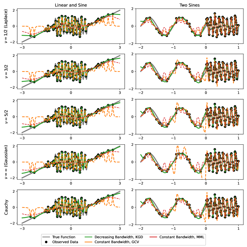
Figure 1: Examples of inferred functions using KGD with decreasing bandwidth and KRR with constant bandwidth and $\lambda$ and $\sigma$ determined through GCV and MML. When the bandwidth is allowed to change during training, all parts of the functions are captured by the model. When a constant bandwidth is used, the inferred function performs well on some parts of the data and poorly on other parts. In the left column, the model selected by GCV performs well on the sinusoidal parts of the function and poorly on the linear parts, and vice versa for the model selected by MML. In the right column, both constant bandwidth models perform well on the high-frequency parts of the function and poorly on low-frequency parts. For some kernels in the right column, the bandwidth selected by GCV is large enough to produce a nearly singular kernel matrix, resulting in cases of extreme predictions between observations, but also small enough for the model to have a tendency to predict zero between observations.

The results for the synthetic data are presented in Table 3. Using a decreasing bandwidth leads to significantly better performance than using a constant one, something that can be attributed to the greater model flexibility. In Figure 1, we display the results of one realization for each data set. We note that when using a constant bandwidth, it tends to be well-adjusted for some parts of the data but either too small or too large for other parts.

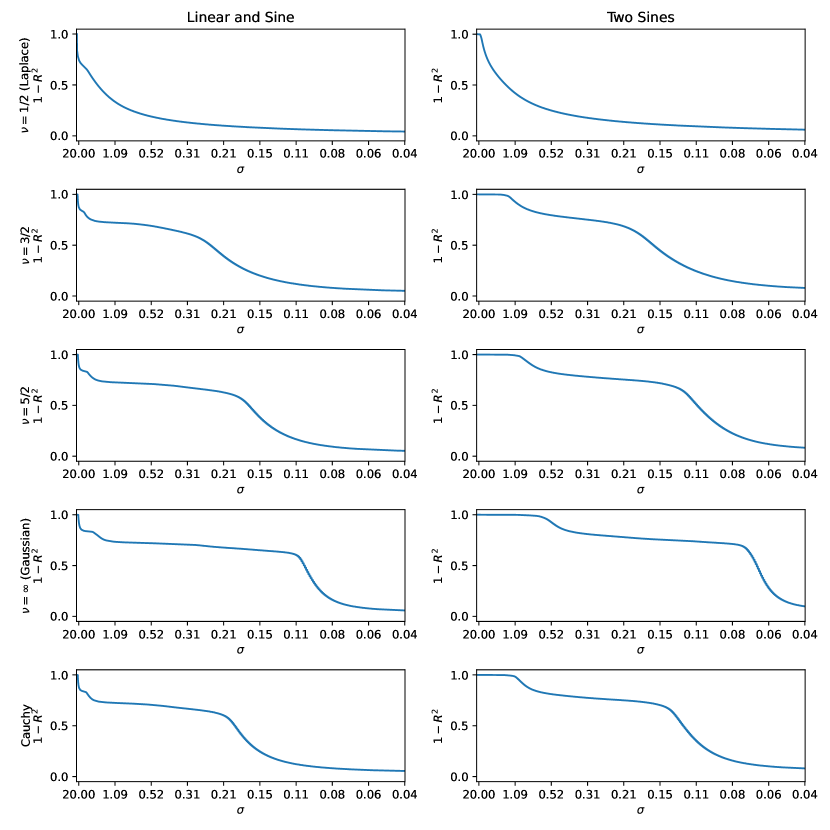
Figure 2: Training error as a function of the bandwidth, which can be used to see which bandwidths are actually used to model the data. In the left column, a large fraction of the training data is explained already for large values of $\sigma$, i.e. when a basically linear model is used. With the exception of the Laplace kernel, a last jump in $R^{2}$ occurs when the bandwidth is approximately between 0.2 and 0.1, which corresponds to $1$ and $1/2$ times the wavelength of the sine wave. In the right column, again with the exception of the Laplace kernel, there are two distinct jumps in $R^{2}$, the first at a bandwidth approximately between 1 and 0.5 and the second approximately between 0.125 and 0.0625, $1$ and $1/2$ times the wavelengths of the two sine waves.

In Figure 2, we demonstrate how the model develops with increasing complexity by plotting the training error as a function of the bandwidth for KGD with decreasing bandwidth. In the left column, where the data is generated as a combination of a linear and a sinusoidal function, much of the data is explained already for a model with low complexity (large bandwidth), i.e. basically a linear model, which is what we expect from a large linear contribution to the true model. The last jump in $R^{2}$ occurs approximately at $\sigma\in[0.2,\ 0.1]$, which can be compared to the wavelength of the sine function, $\frac{1}{5}=0.2$. Thus, the model is complex enough to model the sinusoidal part when the bandwidth is somewhere between the half and the full wavelength. In the right column, where two sine functions of different frequencies were used, we see two jumps in $R^{2}$ at approximately $\sigma\in[1,\ 0.5]$ and $\sigma\in[0.125,\ 0.0625]$, again the half and full wavelengths of the two sine functions.

Table 3: Median and first and third quartile of test $R^{2}$ for 100 simulations for comparisons of the three methods for the five different kernels on the two synthetic data sets. KGD with decreasing bandwidth exhibits significantly higher values of test $R^{2}$ than the competing methods. Its performance is also much more stable with respect to kernel and data.

	Data	Linear and Sine		Two Frequencies
Kernel	Method	Test $R^{2}$ (Q2, (Q1, Q3))	p-value	Test $R^{2}$ (Q2, (Q1, Q3))	p-value
$\nu=1/2$ (Laplace)	KGD	$0.89,\ (0.84,0.91)$	$-$	$0.86,\ (0.83,0.89)$	$-$
	GCV	$0.77,\ (0.71,0.80)$	$7.73\cdot 10^{-18}$	$0.20,\ (-4.46,0.45)$	$1.95\cdot 10^{-18}$
	MML	$0.37,\ (0.26,0.49)$	$1.95\cdot 10^{-18}$	$0.53,\ (0.43,0.61)$	$2.13\cdot 10^{-18}$
$\nu=3/2$	KGD	$0.90,\ (0.87,0.93)$	$-$	$0.87,\ (0.83,0.90)$	$-$
	GCV	$0.47,\ (0.29,0.73)$	$1.95\cdot 10^{-18}$	$0.43,\ (0.27,0.55)$	$2.41\cdot 10^{-18}$
	MML	$0.39,\ (0.34,0.48)$	$1.95\cdot 10^{-18}$	$0.74,\ (0.65,0.79)$	$3.76\cdot 10^{-14}$
$\nu=5/2$	KGD	$0.90,\ (0.87,0.93)$	$-$	$0.87,\ (0.82,0.89)$	$-$
	GCV	$0.34,\ (0.21,0.42)$	$1.95\cdot 10^{-18}$	$0.50,\ (0.32,0.69)$	$5.2\cdot 10^{-17}$
	MML	$0.50,\ (0.36,0.73)$	$5.6\cdot 10^{-13}$	$0.73,\ (0.67,0.77)$	$2.78\cdot 10^{-12}$
$\nu=\infty$ (Gaussian)	KGD	$0.91,\ (0.86,0.94)$	$-$	$0.84,\ (0.78,0.88)$	$-$
	GCV	$0.38,\ (0.32,0.46)$	$2.01\cdot 10^{-18}$	$0.72,\ (0.62,0.77)$	$1.55\cdot 10^{-8}$
	MML	$0.69,\ (0.37,0.77)$	$2.13\cdot 10^{-18}$	$0.70,\ (0.65,0.74)$	$4.23\cdot 10^{-9}$
Cauchy	KGD	$0.90,\ (0.87,0.93)$	$-$	$0.87,\ (0.82,0.90)$	$-$
	GCV	$0.35,\ (0.25,0.45)$	$1.95\cdot 10^{-18}$	$0.43,\ (0.33,0.60)$	$2.88\cdot 10^{-18}$
	MML	$0.58,\ (0.41,0.71)$	$8.41\cdot 10^{-15}$	$0.76,\ (0.70,0.81)$	$2.23\cdot 10^{-10}$

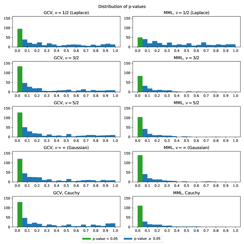
Figure 3: Distributions of p-values for Wilcoxon signed-rank tests, testing whether KGD with decreasing bandwidth performs better than KRR with constant bandwidth and regularization, in terms of test $R^{2}$, on the U.K. temperature data. For the constant models, GCV and MML were used for hyper-parameter selection. The distributions of the p-values are heavily shifted toward the left, with $p<0.05$ for approximately a third of the days.

In Figure 3, we present the distributions of the p-values from testing whether the model with a decreasing bandwidth performs better than the two models with constant bandwidth, on the U.K. temperature data. The distributions of p-values are heavily shifted toward the left, with $p<0.05$ for approximately a third of the days, which means that a decreasing bandwidth results in better performance than a constant bandwidth does.

5.2 Double Descent in Minimum Bandwidth

We demonstrate double descent as a function of model complexity on the U.K. temperature data, and on a synthetic data set by sampling 20 observations according to

$$x\sim\mathcal{U}(-1,1),\ y=\sin(2\pi x)+\mathcal{N}(0,0.2^{2}).$$

For a fixed regularization, $\lambda=1/t=0.001$, KGD with decreasing bandwidth and KRR with constant bandwidth were evaluated for 100 bandwidth values, $\{\sigma_{m}\}_{m=1}^{100}$. For KRR with constant bandwidth, $\sigma_{m}$ was used during the entire training. For KGD with decreasing bandwidth, $\sigma_{m}$ was used as the minimum allowed bandwidth.

In Figures 4 and 5, we plot the training and test errors, as functions of $\sigma_{m}$, for kernel regression with constant and decreasing bandwidths. For large values of $\sigma_{m}$, both models perform poorly both in terms of training and test error. With decreasing $\sigma_{m}$ (increasing model complexity), both the training and test errors decrease, but approximately where the training error becomes zero, the test error starts to increase again. For the constant bandwidth model, the test error continues to increase, but for the decreasing bandwidth model, as the minimum allowed bandwidth becomes even smaller, the test error starts to decrease again. The hump in the error for intermediate model complexities decreases with $\nu$ and is hardly present at all for $\nu=1/2$. This can be attributed to the differentiability of the kernels. For the infinitely differentiable Gaussian kernel, zero training error tends to result in extreme predictions, while for the Laplace kernel, which has discontinuous derivatives, this is not necessarily the case. This is demonstrated in Figure 6, where we plot the inferred functions for one realization for the synthetic data, for four indicative values of $\sigma_{m}$. In the figure, the difference between using a constant and a decreasing bandwidth becomes apparent for small values of $\sigma_{m}$. For a decreasing bandwidth, since simpler models are captured in the early stages of training, a small value of $\sigma_{m}$ can be combined with good generalization. This is, however, not the case if a small bandwidth is used during the entire training. We also see how the Laplace kernel, with discontinuous derivatives, basically performs linear interpolation between the observations, especially for large bandwidths, which explains the absence of a hump in this case.

6 Conclusions

We generalized kernel gradient descent to non-constant kernels and addressed the implications for generalization. Based on our theoretical analysis, we proposed an update scheme for the bandwidth of the kernel during training, obtaining a method that combines zero training error with good generalization. We also related the bandwidth to model complexity and theoretically addressed the phenomenon of double descent as a function of model complexity. We verified our findings by experiments on real and synthetic data.

Kernel regression with non-constant kernels opens up both for better performance on complicated data sets and for a better understanding of generalization as a function of model complexity. An interesting future line of research would be to try to apply our findings to other iteratively trained non-linear regression models. The obvious example would be neural networks, which are also known for combining zero training error with good generalization, and for displaying a double descent behavior.

Code is available at https://github.com/allerbo/non_constant_kgd

Figure 4: Training and test errors (as $1-R^{2}$) as functions of model complexity (as $1/\sigma_{m}$), for kernel regression with constant and decreasing bandwidths. The plots show the median and first and third quartiles from the 366 days. For simple models, both the training and test errors are large, but they all decrease with increasing model complexity. While the training errors decrease toward zero, the test errors start to increase again as the models become even more complex. When using a decreasing bandwidth, there is a second descent in the error as the model complexity increases further, something that is not the case for the constant bandwidth model.

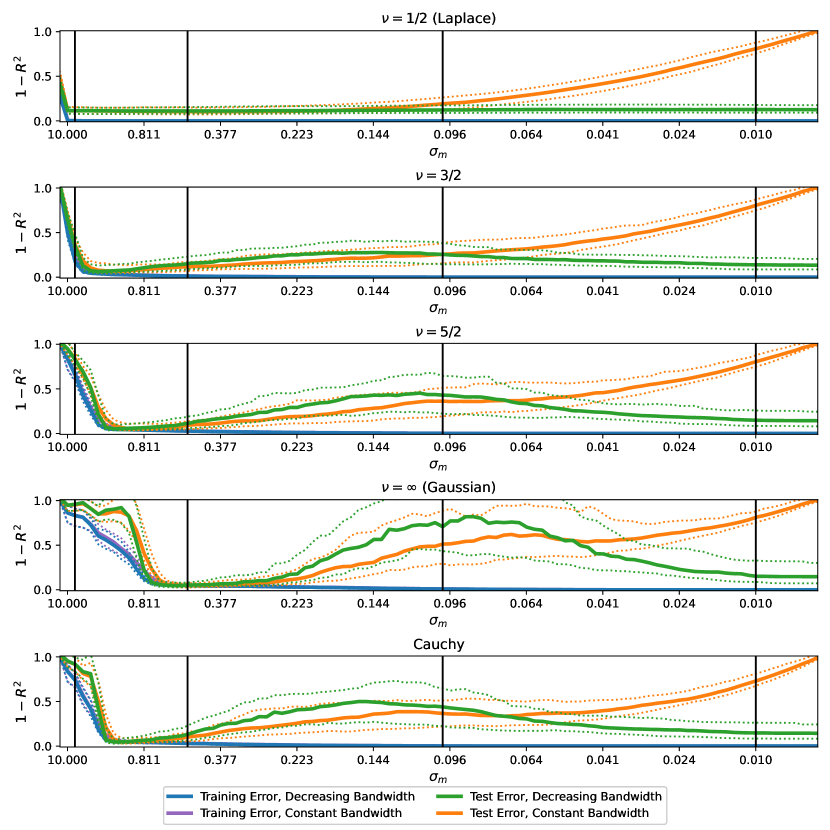
Figure 5: Training and test errors (as $1-R^{2}$) as functions of model complexity (as $1/\sigma_{m}$), for kernel regression with constant and decreasing bandwidths. The plots show the median and first and third quartiles from 100 simulations. For simple models, both the training and test errors are large, but they all decrease with increasing model complexity. While the training errors decrease toward zero, the test errors start to increase again as the models become even more complex. When using a decreasing bandwidth, there is a second descent in the error as the model complexity increases further, something that is not the case for the constant bandwidth model. The black vertical lines correspond to the values of $\sigma_{m}$ used in Figure 6.

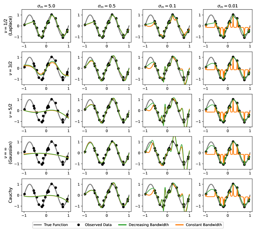
Figure 6: Examples of inferred model for different model complexities, corresponding to the black vertical lines in Figure 5. The Laplace kernel, with discontinuous derivatives, basically performs linear interpolation between the observations. For the four other kernels, in the first column, the models are too simple and perform badly on both training and test data. In the second column, the models do well on both training and test data. In the third column, the models perfectly explain the training data but tend to exhibit extreme predictions between observations. In the fourth column, both models perfectly explain the training data, but in contrast to the decreasing bandwidth model, the constant bandwidth model tends to generalize poorly.

Appendix A Proofs

Proof of Lemma 1.

$$\left|{\bm{k^{*}}}^{\top}(\bm{I}-\exp(-t\bm{K}))\bm{K}^{-1}\bm{y_{\mu}}\right| \leq\|\bm{k^{*}}\|_{2}\cdot\|(\bm{I}-\exp(-t\bm{K}))\bm{K}^{-1}\|_{2}\cdot\|\bm{y_{\mu}}\|_{2}$$

$$=\|\bm{k^{*}}\|_{2}\cdot\frac{1-e^{-t\cdot s_{\min}}}{s_{\min}}\cdot\|\bm{y_{\mu}}\|_{2}$$

$$\leq\|\bm{k^{*}}\|_{2}\cdot\max\left(t,\ \frac{1}{s_{\min}}\right)\cdot\|\bm{y_{\mu}}\|_{2},$$

where in the last equality we used $\|\bm{A}\|_{2}=s_{\max}(\bm{A})$ and the fact that $\frac{1-e^{-t\cdot s}}{s}$ is a decreasing function in $s$, and in the last inequality we used Lemma 3.

$$\left|{\bm{k^{*}}}^{\top}(\bm{K}+\lambda\bm{I})^{-1}\bm{y_{\mu}}\right|\leq\|\bm{k^{*}}\|_{2}\cdot\|(\bm{K}+\lambda\bm{I})^{-1}\|_{2}\cdot\|\bm{y_{\mu}}\|_{2} =\|\bm{k^{*}}\|_{2}\cdot\frac{1}{s_{\min}+\lambda}\cdot\|\bm{y_{\mu}}\|_{2}$$

$$\leq\|\bm{k^{*}}\|_{2}\cdot\max\left(\frac{1}{\lambda},\ \frac{1}{s_{\min}}\right)\cdot\|\bm{y_{\mu}}\|_{2},$$

where in the last equality we used $\|\bm{A}\|_{2}=s_{\max}(\bm{A})$ and $s_{\max}(\bm{A})=1/s_{\min}(\bm{A}^{-1})$, and in the last inequality we used $\lambda,s_{\min}\geq 0$. ∎

Lemma 3.

For $s,t>0$,

$$\frac{1-e^{-ts}}{s}\leq\min\left(t,\ \frac{1}{s}\right).$$

Proof.

That

$$\frac{1-e^{-ts}}{s}\leq\frac{1}{s}$$

follows immediately from $e^{-ts}\in[0,1]$ for $s,t\geq 0$.

To show that

$$\frac{1-e^{-ts}}{s}\leq t,$$

we first show that $\frac{1-e^{-ts}}{s}$ is a decreasing function in $s$:

$$\frac{\partial}{\partial s}\left(\frac{1-e^{-ts}}{s}\right)=\frac{e^{-st}\left(st-e^{st}+1\right)}{s^{2}}.$$

The derivative is non-positive if, for $x=ts$, $x-e^{x}+1\leq 0$. We calculate the maximum by setting the derivative to zero,

$$0=\frac{\partial}{\partial x}\left(x-e^{x}+1\right)=1-e^{x}\implies x=0\implies\max_{x}(x-e^{x}+1)=0-e^{0}-1=0.$$

Thus $\frac{1-e^{-ts}}{s}$ is a decreasing function in $s$, and obtains it maximum in the smallest allowed value of $s$, which is $s=0$:

$$\lim_{s\to 0}\left(\frac{1-e^{-ts}}{s}\right)=\lim_{s\to 0}\left(\frac{1-1+ts+\mathcal{O}(s^{2})}{s}\right)=\lim_{s\to 0}\left(t+\mathcal{O}(s)\right)=t.$$

∎

Proof of Proposition 1.

Using $\frac{\partial\hat{f}_{\mu}(\bm{x^{*}},\tau)}{\partial\tau}=\frac{\partial\hat{f}(\bm{x^{*}},\tau)}{\partial\tau}={\bm{k^{*}}}^{\top}\left(\bm{y}-\bm{\hat{f}}(\tau)\right)$ from Equation 3 and $\left\|\bm{y}-\bm{\hat{f}}(\tau)\right\|_{2}\leq e^{-\tau\cdot\overline{s_{\min}}}\cdot\|\bm{y_{\mu}}\|_{2}$ from Lemma 4, we obtain

$$|\hat{f}_{\mu}(\bm{x^{*}},t)| =\left|\int_{0}^{t}\frac{\partial\hat{f}_{\mu}(\bm{x^{*}},\tau)}{\partial\tau}d\tau\right|\leq\int_{0}^{t}\left|\frac{\partial\hat{f}_{\mu}(\bm{x^{*}},\tau)}{\partial\tau}\right|d\tau=\int_{0}^{t}\left|\bm{k^{*}}(\tau)^{\top}\left(\bm{y}-\bm{\hat{f}}(\tau)\right)\right|d\tau$$

$$\leq\int_{0}^{t}\left\|\bm{k^{*}}(\tau)\right\|_{2}\cdot\left\|\bm{y}-\bm{\hat{f}}\left(\tau\right)\right\|_{2}d\tau=\overline{k^{*}_{2}}\cdot\int_{0}^{t}\left\|\bm{y}-\bm{\hat{f}}\left(\tau\right)\right\|_{2}d\tau$$

$$\leq\overline{k^{*}_{2}}\cdot\int_{0}^{t}e^{-\tau\cdot\overline{s_{\min}}}d\tau\cdot\|\bm{y_{\mu}}\|_{2}=\overline{k^{*}_{2}}\cdot\left(\frac{-1}{\overline{s_{\min}}}e^{-t\cdot\overline{s_{\min}}}+C_{0}\right)\cdot\|\bm{y_{\mu}}\|_{2}$$

$$=\overline{k^{*}_{2}}\cdot\frac{1-e^{-t\cdot\overline{s_{\min}}}}{\overline{s_{\min}}}\cdot\|\bm{y_{\mu}}\|_{2}\leq\overline{k^{*}_{2}}\cdot\min\left(t,\ \frac{1}{\overline{s_{\min}}}\right)\cdot\|\bm{y_{\mu}}\|_{2},$$

where $C_{0}=\frac{1}{\overline{s_{\min}}}$ is calculated from $\hat{f}_{\mu}(\bm{x^{*}},0)=0$ and the last inequality is due to Lemma 3. ∎

Lemma 4.

Let $s_{\min}(\tau)=s_{\min}(\bm{K}(\tau))$ denote the smallest eigenvalue of $\bm{K}(\tau)$ for $\tau\in[0,t]$, and let $\overline{s_{\min}}:=\frac{1}{t}\int_{0}^{t}s_{\min}(\tau)d\tau$ denote its time average. Then

$$\left\|\bm{y}-\bm{\hat{f}}(t)\right\|_{2}\leq e^{-\int_{0}^{t}s_{\min}(\tau)d\tau}\cdot\|\bm{y_{\mu}}\|_{2}=e^{-t\cdot\overline{s_{\min}}}\cdot\|\bm{y_{\mu}}\|_{2}\leq\|\bm{y_{\mu}}\|_{2}.$$

Proof.

The proof is an adaptation of the proof of Theorem 8.2 by Rugh, (1996).

Let $\bm{\hat{\eta}}(t)=\bm{y}-\bm{\hat{f}}(t)$. Then $\bm{\hat{\eta}}(0)=\bm{y_{\mu}}$ and according to Equation 3,

$$\bm{\hat{\eta}}^{\prime}(t)=-\frac{\partial\bm{\hat{f}}(t)}{\partial t}=-\bm{K}(t)\left(\bm{y}-\bm{\hat{f}}(t)\right)=-\bm{K}(t)\bm{\hat{\eta}}(t).$$

Using the chain rule, we obtain

$$\left(\|\bm{\hat{\eta}}(t)\|_{2}^{2}\right)^{\prime}=\left(\bm{\hat{\eta}}(t)^{\top}\bm{\hat{\eta}}(t)\right)^{\prime}=2\bm{\hat{\eta}}(t)^{\top}\bm{\hat{\eta}}^{\prime}(t)=-2\bm{\hat{\eta}}(t)^{\top}\bm{K}(t)\bm{\hat{\eta}}(t)\leq-2\cdot s_{\min}(t)\cdot\|\bm{\hat{\eta}}(t)\|_{2}^{2},$$

where in the last inequality we have used that the Rayleigh quotient of a symmetric matrix, $\bm{A}$, is bounded by its eigenvalues: For all vectors $\bm{v}$,

$$s_{\min}(\bm{A})\leq\frac{\bm{v}^{\top}\bm{A}\bm{v}}{\bm{v}^{\top}\bm{v}}\leq s_{\max}(\bm{A})\iff s_{\min}(\bm{A})\cdot\|\bm{v}\|_{2}^{2}\leq\bm{v}^{\top}\bm{A}\bm{v}\leq s_{\max}(\bm{A})\cdot\|\bm{v}\|_{2}^{2}.$$

Using Grönwall’s inequality on

$$\left(\|\bm{\hat{\eta}}(t)\|_{2}^{2}\right)^{\prime}\leq-2s_{\min}(t)\cdot\|\bm{\hat{\eta}}(t)\|_{2}^{2},$$

we obtain

$$\|\bm{\hat{\eta}}(t)\|_{2}^{2} \leq e^{-2\int_{0}^{t}s_{\min}(\tau)d\tau}\cdot\|\bm{\hat{\eta}}(0)\|_{2}^{2}\iff\|\bm{\hat{\eta}}(t)\|_{2}\leq e^{-\int_{0}^{t}s_{\min}(\tau)d\tau}\cdot\|\bm{\hat{\eta}}(0)\|_{2}$$

$$=\underbrace{e^{-t\cdot\overline{s_{\min}}}}_{\leq 1}\cdot\|\bm{y_{\mu}}\|_{2}\leq\|\bm{y_{\mu}}\|_{2}.$$

∎

Proof of Proposition 2.

Since $\lim_{\sigma\to\infty}\bm{k^{*}}(\sigma)=\bm{1}$, and $\lim_{\sigma\to\infty}\bm{K}(\sigma)=\bm{1}\bm{1}^{\top}$, where $\bm{1}\in\mathbb{R}^{n}$ is a vector of only ones,

$$\lim_{\sigma\to\infty}\hat{f}_{\mu}(\bm{x^{*}},t,\sigma) =\bm{1}^{\top}(\bm{1}\bm{1}^{\top})^{-1}(\bm{I}-\exp(-t\bm{1}\bm{1}^{\top}))\bm{y_{\mu}}=\bm{1}^{\top}(\bm{1}\bm{1}^{\top})^{-1}\left(\bm{I}-\sum_{k=0}^{\infty}\frac{(-t)^{k}}{k!}\underbrace{(\bm{1}\bm{1}^{\top})^{k}}_{=n^{k-1}\cdot\bm{1}\bm{1}^{\top}}\right)\bm{y_{\mu}}$$

$$=\bm{1}^{\top}(\bm{1}\bm{1}^{\top})^{-1}\left(\bm{I}-\frac{1}{n}\cdot\bm{1}\bm{1}^{\top}\cdot\sum_{k=0}^{\infty}\frac{(-tn)^{k}}{k!}\right)\bm{y_{\mu}}=\bm{1}^{\top}\left((\bm{1}\bm{1}^{\top})^{-1}-\frac{1}{n}\cdot e^{-tn}\right)\bm{y_{\mu}}$$

$$\stackrel{{\scriptstyle(a)}}{{=}}\frac{1}{n}\cdot\left(1-\frac{1}{n}\cdot e^{-tn}\right)\bm{1}^{\top}\bm{y_{\mu}}=(1-e^{-tn})\cdot\frac{1}{n}\cdot\sum_{i=1}^{n}y_{\mu,i}=(1-e^{-tn})\cdot\overline{y_{\mu}},$$

where $(a)$ is calculated using the matrix inversion lemma,

$$\bm{D}^{-1}\bm{C}(\bm{A}-\bm{B}\bm{D}^{-1}\bm{C})^{-1}=(\bm{D}-\bm{C}\bm{A}^{-1}\bm{B})^{-1}\bm{C}\bm{A}^{-1},$$

for $\bm{A}=\varepsilon\bm{I}$, $\bm{B}=-\bm{1}$, $\bm{C}=\bm{1}^{\top}$ and $\bm{D}=\bm{I}$:

$$\bm{1}^{\top}(\bm{1}\bm{1}^{\top})^{-1}=\lim_{\varepsilon\to 0}\bm{1}^{\top}(\bm{1}\bm{1}^{\top}+\varepsilon\bm{I})^{-1}=\lim_{\varepsilon\to 0}\bm{1}^{\top}(\bm{I}+\bm{1}^{\top}(1/\varepsilon\bm{I})\bm{1})^{-1}\bm{1}^{\top}(1/\varepsilon\bm{I})=\lim_{\varepsilon\to 0}\frac{1}{\varepsilon+n}\bm{1}^{\top}=\frac{1}{n}\cdot\bm{1}^{\top}.$$

Similarly,

$$\lim_{\sigma\to\infty}\hat{f}_{\mu}(\bm{x^{*}},\lambda,\sigma) =\bm{1}^{\top}(\bm{1}\bm{1}^{\top}+\lambda\bm{I})^{-1}\bm{y_{\mu}}\stackrel{{\scriptstyle(a)}}{{=}}(\bm{I}+\bm{1}^{\top}(1/\lambda\bm{I})\bm{1})^{-1}\bm{1}^{\top}(1/\lambda\bm{I})\bm{y_{\mu}}$$

$$=1/\lambda(\bm{I}+1/\lambda\bm{1}^{\top}\bm{1})^{-1}\bm{1}^{\top}\bm{y_{\mu}}=\frac{1}{\lambda}\cdot\frac{1}{1+n/\lambda}\cdot\sum_{i=1}^{n}y_{\mu,i}$$

$$=\frac{1}{n+\lambda}\cdot\sum_{i=1}^{n}y_{\mu,i}=\frac{n}{n+\lambda}\cdot\overline{y_{\mu}},$$

where $(a)$ is according to the matrix inversion lemma for $\bm{A}=\lambda\bm{I}$, $\bm{B}=-\bm{1}$, $\bm{C}=\bm{1}^{\top}$ and $\bm{D}=\bm{I}$.

We further have $\lim_{\sigma\to 0}\bm{k^{*}}(\sigma)=\begin{cases}\bm{0}\text{ if }\bm{x^{*}}\notin\bm{X}\\ \bm{e_{i}}\text{ if }\bm{x^{*}}=\bm{x_{i}}\in\bm{X},\end{cases}$ where $\bm{e_{i}}$ is a vector of only zeros, except element $i$ which is one, and $\lim_{\sigma\to 0}\bm{K}(\sigma)=\bm{I}$.

Thus, if $\bm{x^{*}}\notin\bm{X}$,

$$\lim_{\sigma\to 0}\hat{f}_{\mu}(\bm{x^{*}},t,\sigma) =\bm{0}^{\top}(\bm{I}-\exp(-t\bm{I}))\bm{I}^{-1}\bm{y_{\mu}}=0$$

$$\lim_{\sigma\to 0}\hat{f}_{\mu}(\bm{x^{*}},\lambda,\sigma) =\bm{0}^{\top}(\bm{I}+\lambda\bm{I})^{-1}\bm{y_{\mu}}=0.$$

If $\bm{x^{*}}=\bm{x_{i}}\in\bm{X}$,

$$\lim_{\sigma\to 0}\hat{f}_{\mu}(\bm{x^{*}},t,\sigma) =\bm{e_{i}}^{\top}(\bm{I}-\exp(-t\bm{I}))\bm{I}^{-1}\bm{y_{\mu}}=(1-e^{-t})\cdot\bm{e_{i}}^{\top}\bm{y_{\mu}}=(1-e^{-t})\cdot y_{\mu,i}$$

$$\lim_{\sigma\to 0}\hat{f}_{\mu}(\bm{x^{*}},\lambda,\sigma) =\bm{e_{i}}^{\top}(\bm{I}+\lambda\bm{I})^{-1}\bm{y_{\mu}}=\frac{1}{1+\lambda}\cdot\bm{e_{i}}^{\top}\bm{y_{\mu}}=\frac{y_{\mu,i}}{1+\lambda}.$$

∎

Proof of Proposition 3.

Mimicking the calculations in the proof of Proposition 1, we obtain

$$\left\|\frac{\partial\hat{f}_{\mu}(\bm{x^{*}},t)}{\partial\bm{x^{*}}}\right\|_{2} =\left\|\int_{0}^{t}\frac{\partial\hat{f}_{\mu}(\bm{x^{*}},\tau)}{\partial\tau\partial\bm{x^{*}}}d\tau\right\|_{2}\leq\int_{0}^{t}\left\|\frac{\partial\hat{f}_{\mu}(\bm{x^{*}},\tau)}{\partial\tau\partial\bm{x^{*}}}\right\|_{2}d\tau$$

$$=\int_{0}^{t}\left\|\frac{\partial}{\partial\bm{x^{*}}}\left(\bm{k}(\bm{x^{*}},\bm{X},\tau)^{\top}\left(\bm{y}-\bm{\hat{f}}(\tau)\right)\right)\right\|_{2}d\tau\leq\int_{0}^{t}\left\|\frac{\partial\bm{k}(\bm{x^{*}},\bm{X},\tau)}{\partial\bm{x^{*}}}\right\|_{2}\cdot\left\|\bm{y}-\bm{\hat{f}}\left(\tau\right)\right\|_{2}d\tau$$

$$=\frac{\int_{0}^{t}\left\|\frac{\partial\bm{k}(\bm{x^{*}},\bm{X},\tau)}{\partial\bm{x^{*}}}\right\|_{2}\cdot\left\|\bm{y}-\bm{\hat{f}}\left(\tau\right)\right\|_{2}d\tau}{\int_{0}^{t}\left\|\bm{y}-\bm{\hat{f}}\left(\tau\right)\right\|_{2}d\tau}\cdot\int_{0}^{t}\left\|\bm{y}-\bm{\hat{f}}\left(\tau\right)\right\|_{2}d\tau$$

$$\leq\frac{\int_{0}^{t}\left\|\frac{\partial\bm{k}(\bm{x^{*}},\bm{X},\tau)}{\partial\bm{x^{*}}}\right\|_{2}\cdot\left\|\bm{y}-\bm{\hat{f}}\left(\tau\right)\right\|_{2}d\tau}{\int_{0}^{t}\left\|\bm{y}-\bm{\hat{f}}\left(\tau\right)\right\|_{2}d\tau}\cdot\min\left(t,\ \frac{1}{\overline{s_{\min}}}\right)\cdot\|\bm{y_{\mu}}\|_{2}.$$

Now, since the covariance matrix $\sigma(\tau)\bm{\Sigma}$, and thus also ${\bm{\Theta}}=\bm{\Sigma}^{-1}$, is positive definite, ${\bm{\Theta}}=\sqrt{{\bm{\Theta}}}\cdot\sqrt{{\bm{\Theta}}}$ and $\left\|\sqrt{{\bm{\Theta}}}\right\|_{2}=\sqrt{\|{\bm{\Theta}}\|_{2}}$,

$$\left\|\frac{\partial\bm{k}(\bm{x^{*}},\bm{X},\tau)}{\partial\bm{x^{*}}}\right\|_{2}=\left\|\frac{\partial}{\partial\bm{x^{*}}}\left(\left[k\left(\frac{\|\bm{x^{*}}-\bm{x_{1}}\|_{\bm{\Theta}}}{\sigma(\tau)}\right),\ k\left(\frac{\|\bm{x^{*}}-\bm{x_{2}}\|_{\bm{\Theta}}}{\sigma(\tau)}\right)\dots,\ k\left(\frac{\|\bm{x^{*}}-\bm{x_{n}}\|_{\bm{\Theta}}}{\sigma(\tau)}\right)\right]\right)\right\|_{2}$$

$$=\left\|\left[k^{\prime}\left(\frac{\|\bm{x^{*}}-\bm{x_{1}}\|_{\bm{\Theta}}}{\sigma(\tau)}\right)\cdot\frac{1}{\sigma(\tau)}\cdot\frac{{\bm{\Theta}}(\bm{x^{*}}-\bm{x_{1}})}{\|\bm{x^{*}}-\bm{x_{1}}\|_{\bm{\Theta}}}\dots,\ k^{\prime}\left(\frac{\|\bm{x^{*}}-\bm{x_{n}}\|_{\bm{\Theta}}}{\sigma(\tau)}\right)\cdot\frac{1}{\sigma(\tau)}\cdot\frac{{\bm{\Theta}}(\bm{x^{*}}-\bm{x_{n}})}{\|\bm{x^{*}}-\bm{x_{n}}\|_{\bm{\Theta}}}\right]\right\|_{2}$$

$$=\left\|\frac{\sqrt{{\bm{\Theta}}}}{\sigma(\tau)}\cdot\left[k^{\prime}\left(\frac{\|\bm{x^{*}}-\bm{x_{1}}\|_{\bm{\Theta}}}{\sigma(\tau)}\right)\cdot\frac{\sqrt{{\bm{\Theta}}}(\bm{x^{*}}-\bm{x_{1}})}{\left\|\sqrt{{\bm{\Theta}}}(\bm{x^{*}}-\bm{x_{1}})\right\|_{2}}\dots,\ k^{\prime}\left(\frac{\|\bm{x^{*}}-\bm{x_{n}}\|_{\bm{\Theta}}}{\sigma(\tau)}\right)\cdot\frac{\sqrt{{\bm{\Theta}}}(\bm{x^{*}}-\bm{x_{n}})}{\left\|\sqrt{{\bm{\Theta}}}(\bm{x^{*}}-\bm{x_{n}})\right\|_{2}}\right]\right\|_{2}$$

$$\leq\underbrace{\max_{u}|k^{\prime}(u)|}_{=:k^{\prime}_{\max}}\cdot\underbrace{\left|\frac{1}{\sigma(\tau)}\right|}_{\sigma(t)\geq 0}\cdot\left\|\sqrt{{\bm{\Theta}}}\right\|_{2}\cdot\left\|\left[\frac{\sqrt{{\bm{\Theta}}}(\bm{x^{*}}-\bm{x_{1}})}{\left\|\sqrt{{\bm{\Theta}}}(\bm{x^{*}}-\bm{x_{1}})\right\|_{2}}\dots,\ \frac{\sqrt{{\bm{\Theta}}}(\bm{x^{*}}-\bm{x_{n}})}{\left\|\sqrt{{\bm{\Theta}}}(\bm{x^{*}}-\bm{x_{n}})\right\|_{2}}\right]\right\|_{2}$$

$$\leq k^{\prime}_{\max}\cdot\frac{1}{\sigma(\tau)}\cdot\left\|\sqrt{{\bm{\Theta}}}\right\|_{2}\cdot\left\|\left[\frac{\sqrt{{\bm{\Theta}}}(\bm{x^{*}}-\bm{x_{1}})}{\left\|\sqrt{{\bm{\Theta}}}(\bm{x^{*}}-\bm{x_{1}})\right\|_{2}}\dots,\ \frac{\sqrt{{\bm{\Theta}}}(\bm{x^{*}}-\bm{x_{n}})}{\left\|\sqrt{{\bm{\Theta}}}(\bm{x^{*}}-\bm{x_{n}})\right\|_{2}}\right]\right\|_{F}$$

$$=k^{\prime}_{\max}\cdot\frac{1}{\sigma(\tau)}\cdot\sqrt{n}\cdot\sqrt{\|{\bm{\Theta}}\|_{2}},$$

where in the last inequality we used $\|\bm{A}\|_{2}\leq\|\bm{A}\|_{F}$, and in the last equality we used that each column in the $n\times p$ matrix has Euclidean norm 1.

Thus,

$$\frac{\int_{0}^{t}\left\|\frac{\partial\bm{k}(\bm{x^{*}},\bm{X},\tau)}{\partial\bm{x^{*}}}\right\|_{2}\cdot\left\|\bm{y}-\bm{\hat{f}}(\tau)\right\|_{2}d\tau}{\int_{0}^{t}\left\|\bm{y}-\bm{\hat{f}}(\tau)\right\|_{2}d\tau}\leq\frac{\int_{0}^{t}k^{\prime}_{\max}\cdot\sqrt{n\cdot\|{\bm{\Theta}}\|_{2}}\cdot\frac{1}{\sigma(t)}\cdot\left\|\bm{y}-\bm{\hat{f}}(\tau)\right\|_{2}d\tau}{\int_{0}^{t}\left\|\bm{y}-\bm{\hat{f}}(\tau)\right\|_{2}d\tau}=k^{\prime}_{\max}\cdot\sqrt{n\cdot\|{\bm{\Theta}}\|_{2}}\cdot\overline{\sigma^{-1}}$$

and

$$\left\|\frac{\partial\hat{f}_{\mu}(\bm{x^{*}},t)}{\partial\bm{x^{*}}}\right\|_{2}\leq\overline{\sigma^{-1}}\cdot\min\left(t,\ \frac{1}{\overline{s_{\min}}}\right)\cdot\|\bm{y_{\mu}}\|_{2}\cdot k^{\prime}_{\max}\cdot\sqrt{n\cdot\|{\bm{\Theta}}\|_{2}}.$$

To prove Equation 10, let $\bm{x^{*}_{\mu}}(t)$ be a value such that $\hat{f}_{\mu}(\bm{x^{*}_{\mu}}(t),t)=0$. Since $\overline{y_{\mu}}=0$, due to continuity, such an $\bm{x^{*}_{\mu}}(t)$ always exists. Then, according to the mean value theorem, for some $\bm{x}(t)\in[\bm{x^{*}},\bm{x^{*}_{\mu}}(t)]$,

$$\left|\hat{f}_{\mu}(\bm{x^{*}},t)\right| =\left|\hat{f}_{\mu}(\bm{x^{*}},t)-\hat{f}_{\mu}(\bm{x^{*}_{\mu}}(t),t)\right|=\left\|\frac{\partial\hat{f}_{\mu}(\bm{x}(t),t)}{\partial\bm{x}(t)}\right\|_{2}\cdot\|\bm{x^{*}}-\bm{x^{*}_{\mu}}(t)\|_{2}$$

$$\leq\overline{\sigma^{-1}}\cdot\min\left(t,\ \frac{1}{\overline{s_{\min}}}\right)\cdot\|\bm{y_{\mu}}\|_{2}\cdot k^{\prime}_{\max}\cdot\sqrt{n\cdot\|{\bm{\Theta}}\|_{2}}\cdot\|\bm{x^{*}}-\bm{x^{*}_{\mu}}(t)\|_{2}$$

$$\leq\overline{\sigma^{-1}}\cdot\min\left(t,\ \frac{1}{\overline{s_{\min}}}\right)\cdot\|\bm{y_{\mu}}\|_{2}\cdot k^{\prime}_{\max}\cdot\sqrt{n\cdot\|{\bm{\Theta}}\|_{2}}\cdot\|\bm{x^{*}}-\bm{x_{m}}\|_{2}.$$

∎

Proof of Lemma 2.

Using the chain rule and $\frac{\partial\bm{\hat{f}_{\mu}}(t)}{\partial t}=\frac{\partial\bm{\hat{f}}(t)}{\partial t}=\bm{K}(t)\left(\bm{y}-\bm{\hat{f}}(t)\right)$ from Equation 3, we obtain

$$\frac{\partial R^{2}(t)}{\partial t}= \left(\frac{\partial R^{2}(t)}{\partial\bm{\hat{f}}(t)}\right)^{\top}\left(\frac{\partial\bm{\hat{f}}(t)}{\partial t}\right)=\frac{2\left(\bm{y}-\bm{\hat{f}}(t)\right)^{\top}}{\left\|\bm{y}-\overline{y}\right\|_{2}^{2}}\bm{K}(t)\left(\bm{y}-\bm{\hat{f}}(t)\right)$$

$$= 2\cdot\frac{\left\|\bm{y}-\bm{\hat{f}}(t)\right\|^{2}_{\bm{K}(t)}}{\left\|\bm{y}-\overline{y}\right\|_{2}^{2}}\geq 0,$$

which proves Equation 12.

To prove Equation 13, we first note that

$$\frac{\partial R^{2}(t)}{\partial t}\cdot\frac{1}{2}\cdot\frac{1}{1-R^{2}(t)} =2\cdot\frac{\left\|\bm{y}-\bm{\hat{f}}(t)\right\|^{2}_{\bm{K}(t)}}{\left\|\bm{y}-\overline{y}\right\|_{2}^{2}}\cdot\frac{1}{2}\cdot\frac{\left\|\bm{y}-\overline{y}\right\|^{2}_{2}}{\left\|\bm{y}-\bm{\hat{f}}(t)\right\|^{2}_{2}}$$

$$=\frac{\left(\bm{y}-\bm{\hat{f}}(t)\right)^{\top}\bm{K}(t)\left(\bm{y}-\bm{\hat{f}}(t)\right)}{\left(\bm{y}-\bm{\hat{f}}(t)\right)^{\top}\left(\bm{y}-\bm{\hat{f}}(t)\right)}.$$

Now, the right hand side of the expression above is the Rayleigh quotient of $\bm{K}(t)$, which is bounded by its singular values, i.e. for any vector $\bm{v}$ and matrix $\bm{A}$, $s_{\min}(\bm{A})\leq\frac{\bm{v}^{\top}\bm{A}\bm{v}}{\bm{v}^{\top}\bm{v}}\leq s_{\max}(A)$. Thus,

$$s_{\min}(\bm{K}(t))\leq\frac{\partial R^{2}(t)}{\partial t}\cdot\frac{1}{2}\cdot\frac{1}{1-R^{2}(t)}\leq s_{\max}(\bm{K}(t)).$$

Finally, for constant $\bm{K}$,

$$\frac{\partial^{2}R^{2}(t)}{\partial t^{2}}= \left(\frac{\partial\frac{\partial R^{2}(t)}{\partial t}}{\partial\bm{\hat{f}}(t)}\right)^{\top}\left(\frac{\partial\bm{\hat{f}}(t)}{\partial t}\right)=\frac{-4\left(\bm{y}-\bm{\hat{f}}(t)\right)^{\top}\bm{K}}{\left\|\bm{y}-\overline{y}\right\|_{2}^{2}}\cdot\bm{K}\left(\bm{y}-\bm{\hat{f}}(t)\right)$$

$$= -4\cdot\frac{\left\|\bm{y}-\bm{\hat{f}}(t)\right\|^{2}_{\bm{K}^{2}}}{\left\|\bm{y}-\overline{y}\right\|_{2}^{2}}\leq 0,$$

which proves Equation 14. ∎

References

- Advani et al., (2020) Advani, M. S., Saxe, A. M., and Sompolinsky, H. (2020). High-dimensional dynamics of generalization error in neural networks. Neural Networks, 132:428–446.
- Ali et al., (2019) Ali, A., Kolter, J. Z., and Tibshirani, R. J. (2019). A continuous-time view of early stopping for least squares regression. In The 22nd International Conference on Artificial Intelligence and Statistics, pages 1370–1378. PMLR.
- Ali et al., (2020) Ali, M., Prasad, R., Xiang, Y., and Yaseen, Z. M. (2020). Complete ensemble empirical mode decomposition hybridized with random forest and kernel ridge regression model for monthly rainfall forecasts. Journal of Hydrology, 584:124647.
- Allerbo, (2023) Allerbo, O. (2023). Solving kernel ridge regression with gradient-based optimization methods. arXiv preprint arXiv:2306.16838.
- Allerbo et al., (2023) Allerbo, O., Jonasson, J., and Jörnsten, R. (2023). Elastic gradient descent, an iterative optimization method approximating the solution paths of the elastic net. Journal of Machine Learning Research, 24(277):1–53.
- Bartlett et al., (2021) Bartlett, P. L., Montanari, A., and Rakhlin, A. (2021). Deep learning: a statistical viewpoint. Acta Numerica, 30:87–201.
- Belkin et al., (2019) Belkin, M., Hsu, D., Ma, S., and Mandal, S. (2019). Reconciling modern machine-learning practice and the classical bias–variance trade-off. Proceedings of the National Academy of Sciences, 116(32):15849–15854.
- Belkin et al., (2018) Belkin, M., Ma, S., and Mandal, S. (2018). To understand deep learning we need to understand kernel learning. In International Conference on Machine Learning, pages 541–549. PMLR.
- Chen and Leclair, (2021) Chen, H. and Leclair, J. (2021). Optimizing etching process recipe based on kernel ridge regression. Journal of Manufacturing Processes, 61:454–460.
- Chen et al., (2022) Chen, Z., Hu, J., Qiu, X., and Jiang, W. (2022). Kernel ridge regression-based tv regularization for motion correction of dynamic mri. Signal Processing, 197:108559.
- Fan et al., (2021) Fan, P., Deng, R., Qiu, J., Zhao, Z., and Wu, S. (2021). Well logging curve reconstruction based on kernel ridge regression. Arabian Journal of Geosciences, 14(16):1–10.
- Friedman and Popescu, (2004) Friedman, J. and Popescu, B. E. (2004). Gradient directed regularization. Unpublished manuscript, http://www-stat.stanford.edu/~ jhf/ftp/pathlite.pdf.
- Friedman, (2001) Friedman, J. H. (2001). Greedy function approximation: a gradient boosting machine. Annals of Statistics, pages 1189–1232.
- Jacot et al., (2018) Jacot, A., Gabriel, F., and Hongler, C. (2018). Neural tangent kernel: Convergence and generalization in neural networks. Advances in Neural Information Processing Systems, 31.
- Jakubovitz and Giryes, (2018) Jakubovitz, D. and Giryes, R. (2018). Improving dnn robustness to adversarial attacks using jacobian regularization. In Proceedings of the European Conference on Computer Vision (ECCV), pages 514–529.
- Kalimeris et al., (2019) Kalimeris, D., Kaplun, G., Nakkiran, P., Edelman, B., Yang, T., Barak, B., and Zhang, H. (2019). Sgd on neural networks learns functions of increasing complexity. Advances in Neural Information Processing Systems, 32.
- Krige, (1951) Krige, D. G. (1951). A statistical approach to some basic mine valuation problems on the witwatersrand. Journal of the Southern African Institute of Mining and Metallurgy, 52(6):119–139.
- Le et al., (2021) Le, Y., Jin, S., Zhang, H., Shi, W., and Yao, H. (2021). Fingerprinting indoor positioning method based on kernel ridge regression with feature reduction. Wireless Communications and Mobile Computing, 2021.
- Ma and Belkin, (2017) Ma, S. and Belkin, M. (2017). Diving into the shallows: a computational perspective on large-scale shallow learning. Advances in Neural Information Processing Systems, 30.
- Mason et al., (1999) Mason, L., Baxter, J., Bartlett, P., and Frean, M. (1999). Boosting algorithms as gradient descent. Advances in Neural Information Processing Systems, 12.
- Matheron, (1963) Matheron, G. (1963). Principles of geostatistics. Economic Geology, 58(8):1246–1266.
- Raskutti et al., (2014) Raskutti, G., Wainwright, M. J., and Yu, B. (2014). Early stopping and non-parametric regression: an optimal data-dependent stopping rule. Journal of Machine Learning Research, 15(1):335–366.
- Rugh, (1996) Rugh, W. J. (1996). Linear System Theory. Prentice-Hall, Inc.
- Safari and Rahimzadeh Arashloo, (2021) Safari, M. J. S. and Rahimzadeh Arashloo, S. (2021). Kernel ridge regression model for sediment transport in open channel flow. Neural Computing and Applications, 33(17):11255–11271.
- Shahsavar et al., (2021) Shahsavar, A., Jamei, M., and Karbasi, M. (2021). Experimental evaluation and development of predictive models for rheological behavior of aqueous fe3o4 ferrofluid in the presence of an external magnetic field by introducing a novel grid optimization based-kernel ridge regression supported by sensitivity analysis. Powder Technology, 393:1–11.
- Singh Alvarado et al., (2021) Singh Alvarado, J., Goffinet, J., Michael, V., Liberti, W., Hatfield, J., Gardner, T., Pearson, J., and Mooney, R. (2021). Neural dynamics underlying birdsong practice and performance. Nature, 599(7886):635–639.
- Wood et al., (2017) Wood, S. N., Li, Z., Shaddick, G., and Augustin, N. H. (2017). Generalized additive models for gigadata: Modeling the uk black smoke network daily data. Journal of the American Statistical Association, 112(519):1199–1210.
- Wu et al., (2021) Wu, Y., Prezhdo, N., and Chu, W. (2021). Increasing efficiency of nonadiabatic molecular dynamics by hamiltonian interpolation with kernel ridge regression. The Journal of Physical Chemistry A, 125(41):9191–9200.
- Yao et al., (2007) Yao, Y., Rosasco, L., and Caponnetto, A. (2007). On early stopping in gradient descent learning. Constructive Approximation, 26(2):289–315.
- Zahrt et al., (2019) Zahrt, A. F., Henle, J. J., Rose, B. T., Wang, Y., Darrow, W. T., and Denmark, S. E. (2019). Prediction of higher-selectivity catalysts by computer-driven workflow and machine learning. Science, 363(6424):eaau5631.
- Zhang et al., (2021) Zhang, C., Bengio, S., Hardt, M., Recht, B., and Vinyals, O. (2021). Understanding deep learning (still) requires rethinking generalization. Communications of the ACM, 64(3):107–115.