TinyFormer: Efficient Transformer Design and Deployment on Tiny Devices

Abstract

Developing deep learning models on tiny devices (e.g. Microcontroller units, MCUs) has attracted much attention in various embedded IoT applications. However, it is challenging to efficiently design and deploy recent advanced models (e.g. transformers) on tiny devices due to their severe hardware resource constraints. In this work, we propose TinyFormer, a framework specifically designed to develop and deploy resource-efficient transformers on MCUs. TinyFormer mainly consists of SuperNAS, SparseNAS and SparseEngine. Separately, SuperNAS aims to search for an appropriate supernet from a vast search space. SparseNAS evaluates the best sparse single-path model including transformer architecture from the identified supernet. Finally, SparseEngine efficiently deploys the searched sparse models onto MCUs. To the best of our knowledge, SparseEngine is the first deployment framework capable of performing inference of sparse models with transformer on MCUs. Evaluation results on the CIFAR-10 dataset demonstrate that TinyFormer can develop efficient transformers with an accuracy of $96.1\%$ while adhering to hardware constraints of $1$MB storage and $320$KB memory. Additionally, TinyFormer achieves significant speedups in sparse inference, up to $12.2\times$, when compared to the CMSIS-NN library. TinyFormer is believed to bring powerful transformers into TinyML scenarios and greatly expand the scope of deep learning applications.

I Introduction

As IoT techniques are becoming increasingly popular recently, microcontroller units (MCUs) have received extensive attention among various kinds of application scenarios. These low-cost, low-power tiny devices are wildly used in plug-and-play scenarios with extreme resource constraints. The devices are usually deployed near the sensor end, gathering the freshest data once produced. Accordingly, Tiny Machine Learning (TinyML) is a growing field in computer science, aiming to apply machine learning technology on MCUs, thereby enabling various applications [1]. Several well-established TinyML applications, such as Keyword Spotting [2], Anomaly Detection and Raise to Wake, only involve some simple deep learning algorithms. Some higher-end applications, such as Wildlife Detection and Food Edibility Detection, usually require powerful deep learning models [3]. However, most of these scenarios only have MCUs available to be exploited, which poses new challenges to TinyML.

Previously, only relatively simple algorithms or lower-end applications were deployed on such tiny devices. If more powerful deep neural networks can be further deployed on tiny devices, it can greatly expand the scope of deep learning applications [4, 5]. However, the available resources of MCUs are strictly limited. For example, ARM Cortex-M7 has only $1$MB storage (Flash) and $320$KB memory (SRAM), compared with some edge devices (such as mobile phones, Raspberry Pi) that have up to GB-level storage and memory. As shown in Fig. 1, there is a large gap between the required resources of deep learning models and the available hardware capacities of tiny devices. For example, deploying ResNet-18 [6] with $11$M parameters into a device with $1$MB storage, at least $90\%$ of weights have to be shrunken, leading to significant accuracy degradation. Therefore, it is difficult to deploy powerful models on such resource-constrained devices.

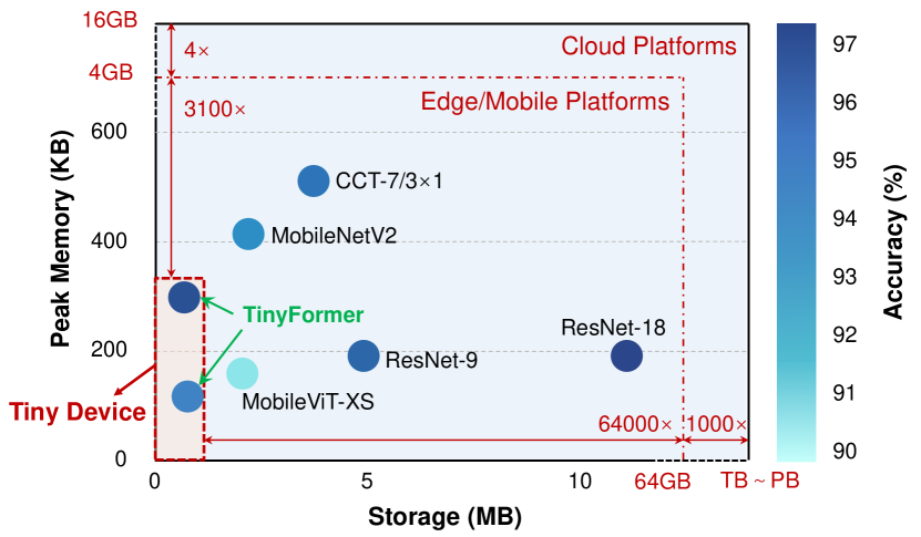
Figure 1: Accuracy and resource usage comparison among different compact models when evaluated on CIFAR-10. Tiny devices only have MB-level storage and KB-level memory, which is a huge difference between the resources available on edge or cloud platforms.

Recently, transformer-based models usually achieve great performance in various fields, such as computer vision, speech recognition and natural language processing [7, 8, 9]. Deploying these powerful transformer models on MCUs can be exciting for satisfying the requirement of high-demanding scenarios in TinyML. However, transformer-based models contain a large number of parameters. Compared with mobile devices and cloud platforms, the available memory and storage are very limited on MCUs. Even for the developed lightweight transformer models [10, 11], it is still difficult to satisfy their strict resource constraints. Therefore, deploying powerful transformer models on edge devices or even MCUs remains difficult.

Aiming to bring powerful transformers to MCUs, TinyFormer is proposed as an efficient framework to design and deploy sparse models with transformers on resource-constrained devices. TinyFormer consists of SuperNAS, SparseNAS and SparseEngine. SuperNAS aims to produce an appropriate supernet from a large search space for further searching. SparseNAS performs model searching in the supernet and model compressing for evaluating hardware constraints and accuracy. SparseEngine automatically optimizes and deploys the compressed models with best accuracy on targeted MCUs. The main contributions of this paper are as follows:

• TinyFormer is proposed as an efficient framework to develop transformers on resource-constrained devices. TinyFormer brings powerful transformers into TinyML scenarios by making it extremely small and efficient on MCUs.

• With the joint search and optimization of sparsity configuration and model architecture, TinyFormer produces a sparse model with best accuracy while satisfying hardware constraints.

• We propose SparseEngine, an automated deployment tool for sparse transformers. To the best of our knowledge, it is the first deployment tool capable of performing sparse inference for models with transformers, with a guaranteed latency on targeted MCUs.

With the cooperation of SuperNAS, SparseNAS and SparseEngine, TinyFormer successfully brings powerful transformers into resource-constrained devices. Experimental results on CIFAR-10 show that TinyFormer could achieve an accuracy of $96.1\%$, with an inference latency of $3.9$ seconds running on STM32F746. Compared to the light-weight transformer CCT-7/3$\times$1 [12], TinyFormer achieves $1.04\%$ accuracy improvement while saving $74\%$ storage. Benefiting from the automated SparseEngine, TinyFormer could obtain up to $12.2\times$ speedup in sparse model inference compared to CMSIS-NN [13].

The rest of the paper is organized as follows. Section II reviews the related background and provides our motivations. Section III demonstrates the details of TinyFormer framework. Experimental results are presented in Section IV and conclusions are given in Section V.

II Related Works and Motivations

Aiming to bring transformers to TinyML scenarios, the following issues have to be comprehensively considered. Firstly, the transformer architecture should be light-weighted to satisfy the extremely demanding resource constraints. Secondly, the sparsity configuration and architecture of the model have coupled effects on accuracy. Thus, we are supposed to consider these effects in the model architecture exploration and compression stage. Finally, it is essential to provide specialized deployment support for targeting on MCUs. These representative investigations motivate us to enable powerful deep-learning models on MCUs through various technological paradigms. Our three primary motivations are listed below:

Motivation ❶ : Design light-weight transformer for MCU.

For TinyML applications, the resources of MCUs are extremely limited. For example, ARM Cortex-M7 STM32F746 has only $1$MB storage and $320$KB memory. Aiming to meet the resource constraints, mixed precision models are deployed on MCUs [14, 15]. However, existing deep neural networks are difficult to satisfy such strict resource constraints. The required storage and peak memory of some light-weight models are illustrated in Fig. 2. Neither MobileNetV2 [16] nor CCT-7/3$\times$1 could satisfy the resource constraints. Therefore, a considerable gap still exists between the limited resources of MCUs and the scales of deep neural networks.

Additionally, some applications require not only the portability and low-power consumption of the MCU, but also its powerful task-specific processing capabilities. Aiming to achieve this goal, a natural approach is to introduce powerful transformers into MCUs. Transformer-based models have demonstrated success in large amount of downstream tasks [7, 8, 9], whereas they usually contain a huge number of parameters. Even the light-weight transformers require resources that are far beyond the upper limit of MCUs constraints [10, 12, 11]. As shown in Fig. 1, both MobileViT-XS [10] and CCT-7/3$\times$1 [12] are beyond the available storage and memory of tiny devices. Therefore, it is challenging to deploy very small transformers onto MCUs. From our perspectives, these efforts will bring transformers into TinyML scenarios, enhancing the applicability of numerous tiny devices.

Motivation ❷ : Joint search with model architecture and sparsity configuration.

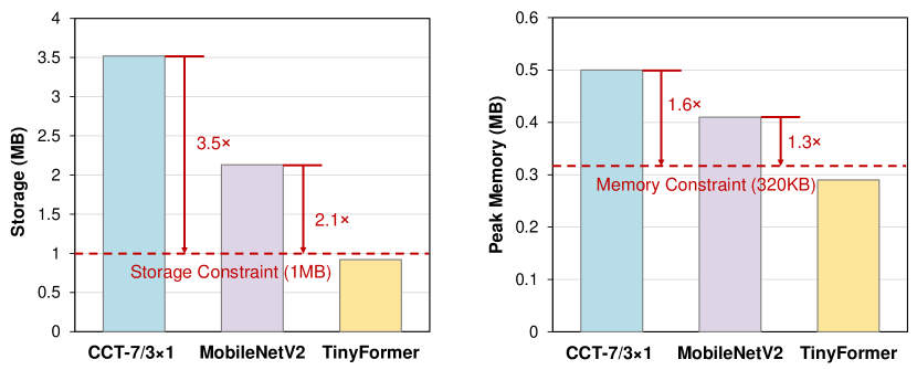
Figure 2: Light-weight models CCT-7/3$\times$1 and MobileNetV2 easily exceed the available hardware resource limits, $\leq 1$MB storage and $\leq 320$KB memory.

Neural Architecture Search (NAS) is an advanced approach in automatically model architecture design [17] and achieves remarkable results in various fields. Most hardware-aware NAS is targeting GPU [18], mobile devices [19, 20] or custom hardware [21]. Currently, there are also some researches exploiting the potential of NAS for light-weight models searching toward IoT devices [22].

Most NAS approaches aim to search for a dense model for better performance. However, the lacking of considering model sparsity in NAS limits the potential benefits of efficient TinyML exploration. Straightforward weight pruning usually causes a significant accuracy drop. Besides, the storage occupation of sparse models includes not only the weights and bias data, but also the cost of sparse coding. It is challenging to balance resource usage and accuracy on TinyML applications.

To address this issue, SpArSe proposed a sparse architecture search algorithm for resource-constrained MCUs [23]. However, SpArSe optimizes the network morphs and performs pruning on respective stages. Hence, it ignores the coupled influence of pruning parameters and network architecture on model accuracy. Aiming to fully consider the interaction between sparsity configuration and dense single-path model, we add pruning steps in two-stage NAS for validation.

Motivation ❸ : Deploy efficient sparse models on MCU.

Model compression can significantly reduce the model size while maintaining accuracy. Accordingly, deploying compressed models on MCUs requires particular support from deployment tools. For example, deployment tools should support sparse model storing and execution to accommodate their extremely perverse resource constraints. Existing deployment tools for MCUs include TensorFlow Lite Micro [24], CMSIS-NN [13], MicroTVM [25], CMix-NN [26] and TinyEngine [27]. However, these frameworks are mainly targeted at small-scale computing by utilizing the locality in dense form for acceleration. None of them support sparse model inference, limiting the scale of models stored in resource-constrained devices. To further exploit the advantage of sparsity, a specialized deployment tool should be developed for sparse model inference on MCUs.

III TinyFormer: A Resource-Efficient Framework

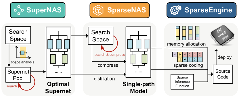
Figure 3: TinyFormer is a hardware-aware framework. SuperNAS is co-designed with SparseNAS to produce sparse models with transformers under resource limits. SparseEngine enables sparse inference on MCUs.

Based on these motivations, we propose TinyFormer, a resource-efficient framework to design and deploy sparse transformer models on resource-constrained devices.

III-A Overview

As shown in Fig. 3, TinyFormer consists of three parts: SuperNAS, SparseNAS and SparseEngine. SuperNAS aims to automatically find an appropriate supernet with transformers in a large search space. In this work, supernet is built as a pre-trained over-parameterized model, where the following single-path models are sampled from the supernet. SparseNAS is adopted to find sparse models with transformer structures from the supernet. Specifically, sparse pruning is performed in convolution and linear layers, and full-integer quantization with INT8 format is applied on all layers. The sparse pruning configurations and compression operations are performed together in the searching stage of SparseNAS. Finally, SparseEngine deploys the obtained model to MCUs with sparse configurations, enabling sparse inference to save hardware resources. SparseEngine could automatically generate binary code for running on STM32 MCUs with several functional implementations to support efficient sparse inference.

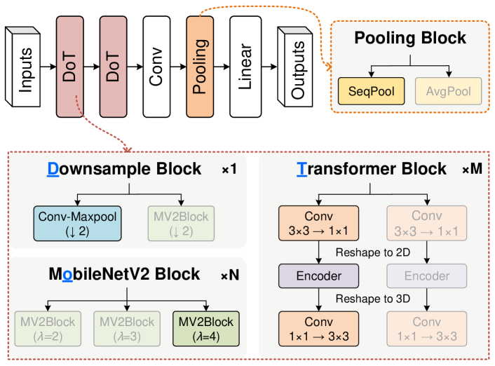
Figure 4: Our supernet architecture design. We design four types of choice blocks: Downsample Block, MobileNetV2 Block, Transformer Block and Pooling Block. Each choice block contains $2$ or $3$ architecture candidates inside. The single-path model is sampled from the supernet with only one architecture candidate invoked per choice block.

III-B SuperNAS: Supernet Architecture Search

When designing a supernet structure to search models and deploy on MCUs, we are facing a trade-off between model sparsity and capacity. The accuracy of smaller dense model is usually limited by capacity, while pruning with higher sparsity on larger model could lead to a drastic drop in accuracy. The balance between model sparsity and capacity should shift according to hardware resource constraints, challenging the design of supernet.

Therefore, we propose SuperNAS to automatically design the supernet. SuperNAS does not directly output the best single-path model. Instead, it searches an appropriate subset from search space and builds a smaller supernet. Loosely speaking, appropriate supernet should satisfy two following conditions. Firstly, most of sparse models obtained from supernet are supposed to satisfy the resource constraints strictly. Secondly, the average validation accuracy of these models should be achieved as high as possible.

With the design of the search space for supernet, SuperNAS first analyses the probability to accept the designed search space. Then SuperNAS randomly samples supernet configurations from search space and evaluates the average accuracy of the random-sampled sparse model in supernet. The supernet with best accuracy will be sent to SparseNAS for actual single-path model search.

1

2

3Input: Search space $\mathbb{S}_{sup}$, memory limit ${\cal L}_{m}$ and storage limit ${\cal L}_{s}$, lower bound ratio $\lambda_{lo}$ and upper bound ratio $\lambda_{up}$, iteration count ${\cal T}_{sup}$.

4

5Output: Probability to accept $\mathbb{S}_{sup}$ for search space.

6 $[n_{accpt},n_{eval}]\leftarrow[0,0]$

7 for $i=1$ to ${\cal T}_{sup}$ do

8       Sample single-path model ${\cal M}^{i}$ from $\mathbb{S}_{sup}$

9      

10      Sample sparse config $c_{sp}^{i}$from $\mathbb{S}_{sup}$

11      

12      $[l_{m}^{i},l_{s}^{i}]$ $\leftarrow$ $ResourceEval({\cal M}^{i},c_{sp}^{i})$

13      

14      if $l_{m}^{i}$ $\leq$ ${\cal L}_{m}$ and $l_{s}^{i}$ $\leq$ ${\cal L}_{s}$ then

15             $n_{eval}$ $\leftarrow$ $n_{eval}+1$

16             $N_{param}^{i}$ $\leftarrow$ $CountModelParam({\cal M}^{i})$

17             if $\lambda_{lo}{\cal L}_{m}$ $\leq$ $N_{param}^{i}$ $\leq$ $\lambda_{up}{\cal L}_{m}$ then

18                   $n_{accpt}$ $\leftarrow$ $n_{accpt}+1$

19                  

20             end if

21            

22       end if

23      

24 end for

25return $n_{accpt}/n_{eval}$

Algorithm 1 Search Space Analysis in SuperNAS

1

2Input: Search space $\mathbb{S}_{sup}$, memory limit ${\cal L}_{m}$ and storage limit ${\cal L}_{s}$, iteration count ${\cal T}_{i}$, ${\cal T}_{j}$ and ${\cal T}_{k}$.

3 Output: An optimal supernet ${\cal A}_{sup}$.

4 for $i=1$ to ${\cal T}_{i}$ do

5       Sample supernet ${\cal A}^{i}$ from $\mathbb{S}_{sup}$

6      

7      if $TestSupernet({\cal A}^{i})\neq True$ then

8             continue

9       end if

10      Train ${\cal A}^{i}$ for $10$ epochs

11       for $j=1$ to ${\cal T}_{j}$ do

12             Sample single-path model ${\cal M}^{i,j}$ from ${\cal A}^{i}$

13             for $k=1$ to ${\cal T}_{k}$ do

14                   Sample sparsity config $c_{sp}^{k}$ from $\mathbb{S}_{sup}$

15                  

16                  $[l_{m},l_{s}]$ $\leftarrow$ $ResourceEval({\cal M}^{i,j},c_{sp}^{k})$

17                   if $l_{m}$ $>$ ${\cal L}_{m}$ or $l_{s}$ $>$ ${\cal L}_{s}$ then

18                         continue

19                   end if

20                  ${\cal M}_{prun}^{i,j,k}\leftarrow OneShotPrune({\cal M}^{i,j},c_{sp}^{k})$

21                   $Acc\leftarrow AccuracyEval({\cal M}_{prun}^{i,j,k})$

22                   $AvgAcc^{i,j}\leftarrow UpdateAvgAcc(Acc)$

23             end for

24            $AvgAcc^{i}\leftarrow UpdateAvgAcc(AvgAcc^{i,j})$

25            

26       end for

27      ${\cal A}_{sup}\leftarrow UpdateBestSupernet({\cal A}^{i},AvgAcc^{i})$

28      

29 end for

30return ${\cal A}_{sup}$

Algorithm 2 Supernet Architecture Seach

III-B1 Search Space of SuperNAS

The search space of SuperNAS contains hyper-parameters that are related to the supernet architecture design, including choices of blocks and number of channels in each choice block. The supernet architecture design is shown in Fig. 4. The supernet architecture design in TinyFormer is similar to the single-path-one-shot (SPOS) approaches [28]. Supernet consists of variate choice blocks, and the single-path model is samples at granularity of choice blocks. We build supernet architecture based on four types of choice blocks: Downsample block, MobileNetV2 block, Transformer block and Pooling block. The four types of blocks contain multiple different architecture candidates respectively.

In Fig. 4, Conv represents a standard $3$$\times$$3$ convolution with $1$$\times$$1$ padding, unless stated otherwise. In Downsample block, Conv-Maxpool refers to a standard convolution following a $2\times 2$ max pooling. Architecture candidates that perform downsampling are tagged with $\downarrow 2$. MobileNetV2 block refers to inverted residual block in [16] with expansion factor $\lambda$. In Transformer block, Conv $3$$\times$$3$$\rightarrow$$1$$\times$$1$ is a standard $3$$\times$$3$ convolution following a $1$$\times$$1$ convolution with no padding. Conv $1$$\times$$1$$\rightarrow$$3$$\times$$3$ is similar to the expression above. Encoder is a standard transformer encoder similar to [9], with ReLU [29] as the activation operation for efficient calculation on MCUs. SeqPool and AvgPool in Pooling block indicate sequence pooling in [12] and $2$$\times$$2$ average pooling, respectively. The single-path model is sampled from the supernet with only one architecture candidate invoked per block, similar to [28].

Unlike CNNs, transformers lack some spatial inductive biases and rely heavily on massive datasets for large-scale training. Therefore, we insert MobileNetV2 block before transformer block to address this issue. The memory usage is sensitive to the size of encoder’s input. To avoid the number of channels being limited by the size of encoder’s input, referring to MobileViT [10], we insert $3$$\times$$3$ convolution and $1$$\times$$1$ convolution before and after the encoder. By this way, we can decouple the relationship between channels and encoder’s input, thus expanding the search space to explore larger scale of candidate models.

We take DoT, an architecture stacked by Downsample block, MobileNetV2 block and Transformer block, as the backbone of the supernet. Furthermore, MobileNetV2 block and Transformer block in DoT structure are repeatable, which makes DoT a more flexible feature extraction architecture. The supernet architecture adopts two DoTs as the backbone, followed by some post-processing operators.

III-B2 Search Space Analysis

The search space of SuperNAS contains hyper-parameters of the supernet, including the number of layers in each choice block, hyper-parameters of architecture candidates, etc. The final single-path model is sampled from the supernet.

As mentioned in III-B, the balance between model sparsity and capacity is essential in search space design, and the configurations of search space determine the supernet and single-path model architecture. Therefore, we need to evaluate search space before sampling supernet. Algorithm 1 shows how we analyze the search space. Before the analysis, we set the hyper-parameter $\lambda_{lo}$ and $\lambda_{up}$ as the lower and upper bound of the single-path model’s capacity. We randomly sample configurations from the search space and build sparse single-path models. If the sparse single-path model meets the hardware constraint, we evaluate the count of parameters in the model and accept the model if the count is between the given boundary. Finally, we calculate the statistical probability to represent how many sampled single-path models are acceptable in the search space. If the statistic probability is higher than $90\%$, we accept the search space for further deployment. Otherwise, we adjust the search space in advance to avoid unnecessary searches.

1 Input: Search space $\mathbb{S}_{sin}$, supernet architecture ${\cal A}$, memory limit ${\cal L}_{m}$ and storage limit ${\cal L}_{s}$, iteration count ${\cal T}_{sin}$.

2 Output: An optimal pruned single-path model ${\cal M}_{prun}$ with its sparse configuration $c_{sp}$.

3 for $i=1$ to ${\cal T}_{sin}$ do

4       Sample single-path model ${\cal M}_{sin}^{i}$ from ${\cal A}$

5       Sample sparsity config $c_{sp}^{i}$ from $\mathbb{S}_{sin}$

6       $[l_{m},l_{s}]$ $\leftarrow$ $ResourceEval({\cal M}^{i},c_{sp}^{i})$

7       if $l_{m}$ $>$ ${\cal L}_{m}$ or $l_{s}$ $>$ ${\cal L}_{s}$ then

8             continue

9       end if

10      Train ${\cal M}^{i}$ for 10 epochs

11       ${\cal M}_{prun}^{i}\leftarrow IterativePrune({\cal M}^{i},c_{sp}^{i})$

12       $Acc^{i}\leftarrow AccuracyEval({\cal M}_{prun}^{i})$

13       ${\cal M}_{prun}\leftarrow UpdateBestModel({\cal M}_{prun}^{i},Acc^{i})$

14       $c_{sp}\leftarrow UpdateSparseConfig(c_{sp}^{i},Acc^{i})$

15      

16 end for

Return ${\cal M}_{prun}$, $c_{sp}$

Algorithm 3 Single-path Model Search in SparseNAS

We conducted experiments in three types of search space: small, normal and large, which denote the model size sampled from them. Detailed experiments of search space analysis can be found in Section IV-B.

III-B3 Supernet Architecture Search

The supernet architecture search process is shown in Algorithm 2. For each supernet built by hyper-parameters sampled from the search space, we perform a simple test on the supernet before the actual search (expressed as TestSupernet in Algorithm 2). Specifically, we randomly sample 100 single-path models from the supernet, and evaluate the memory usage of each model. If half of the models exceed the memory limit of hardware constraint, we skip the search procedure for supernet.

After the simple test of supernet, we take two steps to evaluate its sensitivity to sparsity. Firstly, we randomly sample single-path models from the supernet. For each single-path model, compression is conducted by randomly generated groups of sparse configuration for checking whether the model occupies more resources than the practical scenario. Then we take the average accuracy of these sparse models as the performance metric of the single-path model. Meanwhile, the average metric of all single-path models is adopted as the final performance metric of supernet. The supernet with the highest performance metric will be adopted for the next search stage.

In order to reduce the search cost, we evaluate the storage and peak memory usage of the sparse models for skipping the ones that do not satisfy the resource requirements. In addition, one-shot pruning algorithm with fine granularity is adopted instead of accurate iterative pruning to reduce the runtime cost.

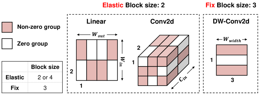
Figure 5: Blockwise pruning method. Here, Linear is a linear layer and Conv2d is a convolution layer. We abbreviate depthwise convolution as DW-Conv2d. $W_{in}$ and $W_{out}$ denote the dimensions of linear layer, $C_{in}$ means the number of input channels and $W_{width}$ is the kernel width of depthwise convolution.

III-C SparseNAS: Hardware-Aware Sparse Network Search

SparseNAS aims to obtain a good single-path model with sparse configuration and path choice encoding from supernet. The single-path model is extracted from the supernet based on the path selection encoding. After the model compression with sparse configuration and fine-tuning with some epochs, the accuracy could be recovered as a satisfiable level. By repeating the above procedures we could obtain the model with the highest accuracy.

The single-path model searching method is similar to SPOS approaches [28]. Excepting the original approaches, the compression procedure is performed including pruning and quantization among searching steps. Moreover, aiming to reduce the cost of training and compression procedures, SparseNAS is divided into two stages, i.e. Two-stage NAS. In first stage, SparseNAS aims to find the best sparse single-path model with pruning and quantization procedures. For the second stage, SparseNAS only performs fine-tuning pruning and operations to recover the model’s accuracy.

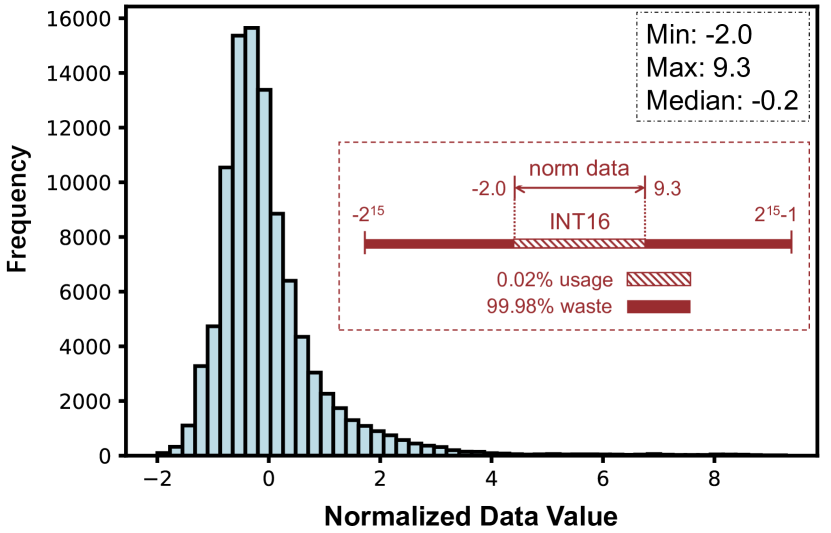
(a)

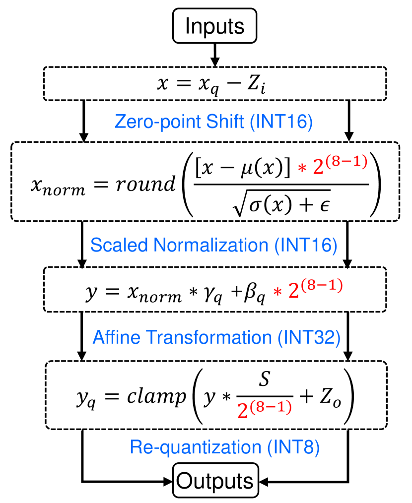
(b)

Figure 6: (a) Distribution of normalized activation in the first layernorm layer. (b) Scaled-LayerNorm inference process. $S$ and $Z$ refer to the scaled and zero-point parameter of quantization respectively. $clamp$ function clamps the result to range of signed INT8.

III-C1 Two-stage NAS

SparseNAS consists of single-path model selection stage and fine-tuning stage. The first stage of SparseNAS is presented in Algorithm 3 for single-path model selection. In first stage, SparseNAS trains randomly-sampled sparse single-path models for a few epoch, then performing iterative pruning and accuracy evaluation. Only the model with highest accuracy will be selected and sent to second stage for further training. We skip the model candidates that do not satisfy hardware constraints by evaluating the storage and memory usage.

For the second stage, SparseNAS only performs iterative pruning and fine-tuning on the model selected from the first stage for accuracy improvement. After the second stage, the fine-tuned model will be sent to SparseEngine for efficient deployment. Two-stage procedures could reduce the training and compression cost while maintaining the obtained single-path model’s accuracy.

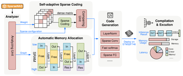
Figure 7: The workflow overview of SparseEngine. Sparse models obtained from SparseNAS are first analyzed for sparse coding and memory allocation. Then, different kinds of layers’ computations are transformed via automatic code generation for the following compilation and execution on targeted MCUs.

III-C2 Pruning Method

Different from the one-shot pruning method in SuperNAS, AGP iterative pruning method [30] is utilized in two-stage NAS. AGP method can avoid significant accuracy degradation caused by pruning. We only perform weight pruning in convolution and linear layers.

SparseNAS adopts a blockwise pruning method, grouping multiple continuous weights as a block to prune. Pruning configuration (sparsity and block size) affects both accuracy and hardware resource usage in deployment, and different layers have different sensitivities to pruning configuration. Therefore, we adopt a mixed-blockwise pruning strategy in Conv and FC layers, as shown in Fig. 5. In mixed-blockwise pruning procedure, SparseNAS select elastic block size (2 or 4) for each layer to prune. Accordingly, we add the pruning confuguration for each choice block into search space. When sampling the single-path model, each choice block is set to a random configuration of sparsity and block size.

As an exception, the block size of depthwise convolution is fixed to $3$. In SparseEngine, we applied the blockwise convolution in width direction to exploit spatial locality in computation. Therefore, the block size of blockwise convolution is set to $3$, for the kernel size is fixed to $3$$\times$$3$.

III-C3 Quantization Method

Floating-point calculations on MCUs are inferior in latency and power efficiency compared to integer calculations. Therefore, we quantize the model weights and activations to INT8 by Post-Training Quantization (PTQ) algorithm [31]. However, LayerNorm calculations in transformer cannot be directly quantized. Performing linear quantization on LayerNorm will cause a significant accuracy drop. The original LayerNorm is defined as:

$$y=\frac{x-\mu(x)}{\sqrt{\sigma(x)+\epsilon}}*\gamma+\beta,$$ (1)

where $\mu(x)=\frac{1}{c}\Sigma^{c}_{i=1}x_{i}$ and $\sigma(x)=\sqrt{\frac{1}{c}\Sigma^{c}_{i=1}(x_{i}-\mu)^{2}}$ are the mean and variance values of input $x$ in channel-wise direction ($c$ is the number of channels). $x_{norm}=\frac{x-\mu(x)}{\sqrt{\sigma(x)+\epsilon}}$ is the normalization result before affine transformation. $\gamma$ and $\beta$ are the learnable parameters in affine transformation. $\epsilon$ is a significantly small value to prevent the denominator to be zero. In linear quantization, the normalization result $x_{norm}$ is supposed to be rounded to integer. However, directly rounding $x_{norm}$ to INT16 incurs a significant loss of precision.

To verify the conjecture, we count the distribution of $x_{norm}$ of LayerNorm in first DoT Architecture. As shown in Fig. 6(a), the normalized data is mapped to the range of $-2.0$ to $9.3$. Rounding the small range of normalization results to INT16 causes a large loss of precision. On the other hand, the range of INT16 is not fully utilized by $x_{norm}$. Adopting INT16 to store the normalized data will waste $99.98\%$ of integer values, presented in Fig. 6(a).

Aiming to tackle this problem, Scaled-LayerNorm is proposed to perform integer-only inference instead of LayerNorm. As shown in Fig. 6(b), we enlarge the normalized results by $2^{(8-1)}$ to reduce the numeric precision loss in quantization. After the linear transformation, the results are stored as INT16 format, while it also includes the $2^{(8-1)}$ factor. In re-quantization step, we fold $\frac{1}{2^{(8-1)}}$ into scaling factor $S$ to ensure mathematical equivalence. Expanding the numerical range of $x_{norm}$ prevents significant accuracy drop caused by large precision loss. With the approaches above, we reach a significant speed-up in LayerNorm inference, with only slight accuracy drop.

III-D SparseEngine: Efficient Deployment of Sparse Models

SparseEngine is an automatic deployment tool for sparse transformer models on MCUs. Comprehensive details of SparseEngine are illustrated in Fig. 7.

Firstly, the models obtained from SparseNAS are analyzed to extract the required information, including sparse configuration, model architecture and memory usage, etc. Aiming to efficiently utilize the available memory on MCUs, a head-tail-alternation allocation strategy is adopted to automatically allocate memory for models inference. Meanwhile, we perform the self-adaptive sparse strategy with blockwise run-length coding in UINT8. Specifically, weights are encoded by the format of $(d,v_{1},v_{2},...,v_{b})$, where $d$ represents the distance between non-zero blocks as the position information, and $v_{i}$ indicates the $i$-th weight in the non-zero block whose length is $b$. With self-adaptive strategy, weights are stored as sparse format only if sparse coding could reduce the storage occupation. Finally, targeted codes could be generated for deployment on MCUs. Kinds of essential operators are implemented for deploying sparse transformer models, including Scaled-LayerNorm, sparse convolution and sparse linear layers.

Compared with other deployment approaches on MCUs, SparseEngine aims to further exploit the sparsity on TinyML deployment and model inference. The sparsity exploitation includes sparse encoding/decoding, and sparse calculations (both Conv and FC layers). Moreover, targeting on model inference with transformer blocks, Softmax operator is also optimized to accelerate the inference on MCUs.

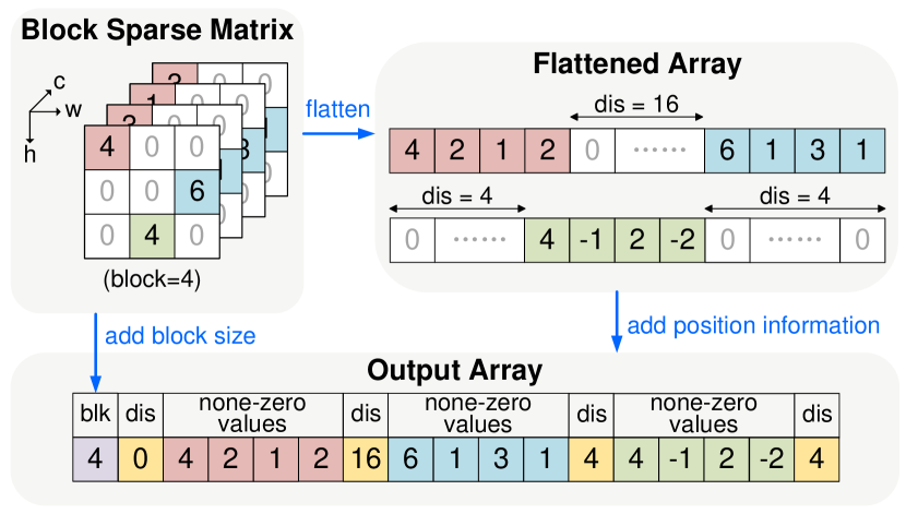
Figure 8: Blockwise run-length coding for 3D matrix.

III-D1 Sparse Coding

In sparse coding, we perform blockwise run-length coding in 8-bit to adopt block pruning. The original 3D matrix (tensor) is firstly flattened into array format. The spare weights are stored in $(dis,val_{1},val_{2}...,val_{b})$ format, as presented in Fig. 8, where $dis$ represents the distance between non-zero blocks as the position information, $val_{i}$ indicates the $i$-th weight in the non-zero block whose length is $b$. We insert zero elements if $dis$ cannot be represented by INT8.

Compared with Coordinate (COO) and Compressed Sparse Row (CSR) formats, blockwise run-length coding has a higher compression ratio. We only require one element to represent the position of adjacent $b$ non-zero weights. The compression ratio of this encoding format could be obtained by

$$\eta=\frac{1}{(1-\rho)\times(1+\frac{1}{b})},$$ (2)

where $\eta$ indicates the compression ratio, $\rho$ refers to the sparsity and $b$ is the block size of pruning. Consequently, the compression ratio of blockwise run-length encoding could be larger along with the increasing of sparsity and block size. Cooperating with mixed-blockwise pruning in SparseNAS, blockwise run-length encoding significantly reduce the required size of sparse coding.

III-D2 Sparse Convolution

Decoding sparse weights and then computing convolution in dense format usually occupies a large amount of memory footprint [32, 33]. To avoid unnecessary memory usage, we perform sparse convolution calculation directly in sparse format. Fig. 9 presents the details of the sparse Conv calculation. Sparse weights are decoded to obtain the coordinates and values. Each weight value corresponds to a sub-matrix of the input matrix. After extracting the sub-matrix, we perform element-matrix multiplication and accumulate the results as the output. Specifically, we decode two weight values simultaneously and extract two corresponding elements from the sub-matrix. Then, two INT8 values are sign-extended to INT16 and concatenated as INT32 format. Thus, the above multiply-accumulate calculations can be performed by SIMD instructions. Meanwhile, the sparse linear layers are implemented by the same manner, despite the difference in dimensions.

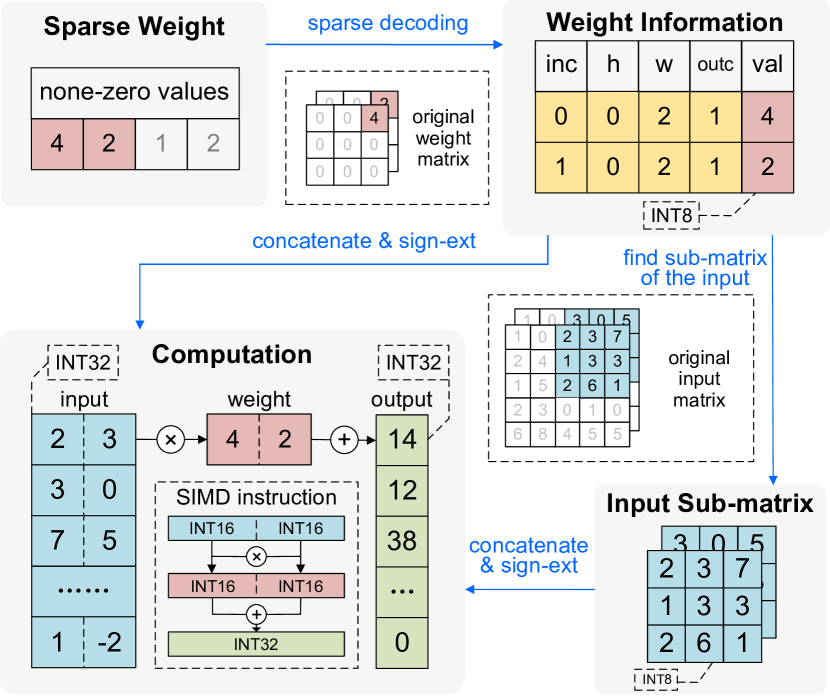
Figure 9: Sparse Convolution with SIMD instruction. Each block’s weight information are extracted by sparse decoding procedure. Among them, the location information are adopted to find the sub-matrix in original input matrix. After concatenate & sign-ext operations, sub-matrix and weight values are sent for computations with SIMD instructions acceleration.

TABLE I: Accuracy comparison and hardware resources evaluation. Different models are evaluated under different hardware constraints. TinyFormer-120K and TinyFormer-300K indicate that the peak memory limit is set as $120$KB and $300$KB, respectively.

Model	Peak Memory	Satisfy Memory	Storage	Satisfy Storage	Top-1 Accuracy
ResNet-18 [6]	$192$KB	✓	$10.66$MB	✗	$96.52$%
MobileNetV2 [16]	$416$KB	✗	$2.13$MB	✗	$94.61$%
MobileViT-XS [10]	$160$KB	✓	$1.91$MB	✗	$90.11$%
CCT-7/3$\times$1 [12]	$512$KB	✗	$3.52$MB	✗	$95.06$%
TinyFormer-120K (ours)	$120$KB	✓	$0.94$MB	✓	$94.52$%
TinyFormer-300K (ours)	$300$KB	✓	$0.91$MB	✓	$96.10$%

III-D3 Softmax Optimization

According to our profiling, the Softmax layer is very time-consuming due to the required exponential operations. The computation of Softmax can be described as

$$Softmax(x_{i})=\frac{e^{x_{i}}}{\sum_{j=1}^{n}e^{x_{j}}}=\frac{e^{x_{i}-x_{max}}}{\sum_{j=1}^{n}e^{x_{j}-x_{max}}},$$ (3)

where $x_{i}$ indicates the $i$-th value and $x_{max}$ indicates the maximum value ($n$ is the number of elements in one channel). Since the inputs of Softmax are INT8 format, the exponents range from -$256$ to $0$. Consequently, redundant calculations will be increased according to the input size of Softmax. Therefore, we optimize the Softmax operator with a lookup table to reduce redundant computations.

Aiming to calculate the negative exponential functions, SparseEngine adopts the absolute value of the exponential factor as an index to query the bitmap. If the corresponding bit has been existed, SparseEngine obtains the result from the lookup table and reuses it in Softmax computations. Otherwise, it calculates the exponential function and stores the result in the table, updating the corresponding bit in the bitmap. According to the evaluation of SparseEngine, its memory usage on bitmap and lookup table is usually less than $1.2$KB. Since we could reuse the buffer memory of convolution when performing Softmax optimization, there is no extra memory cost in calculations.

IV Experimental Results

IV-A Evaluation Setup

IV-A1 Dataset

According to TinyML scenario’s requirements, our TinyFormer is mainly evaluated on CIFAR-10 [34] dataset for image classification. Unless otherwise specified, all involved models are trained from scratch for $300$ epochs using a batch size of $128$.

IV-A2 Training Settings

The adopted optimizer is AdamW [35]. The learning rate starts with a warm-up phase, increasing from $1e^{-5}$ to $55e^{-5}$ for the first $10$ epochs, and then follows a cosine annealing schedule, gradually decreasing to $0.1$. During model’s training, label smoothing with a probability of $0.1$ is employed, as suggested by Szegedy et al. [36].

IV-A3 Models

Since ResNet-18 [6], MobileNetV2 [16] and MobileViT-XS [10] were originally designed for ImageNet dataset [37], we made modifications to their initial layers to accommodate the image size of CIFAR-10. To ensure a fair comparison, all models are performed INT8 quantization and all reported top-1 accuracy values are tested on quantized models if not specifically stated.

IV-A4 Platforms

All experiments are conducted on a MCU platform with Cortex-M7 STM32F746 ($320$KB Memory and $1$MB Storage) inside for accuracy and efficiency evaluation.

IV-B Offline Evaluation

Table I shows the comparison results among our TinyFormer and other state-of-the-art models. With the co-optimization of SuperNAS and SparseNAS, our TinyFormer-300K could satisfy hardware constraints and achieve a record accuracy ($96.1\%$) with CIFAR-10 on MCUs. As illustrated in Fig. 4, TinyFormer is designed as a hybrid model that contains both convolution and transformer encoder layers. Compared to other light-weight hybrid models, such as MobileViT-XS and CCT-7/3$\times$1 [12], TinyFormer better combines the advantages of CNN and transformer to achieve higher accuracy with limited resources. Compared with CCT-7/3$\times$1 designed for CIFAR-10, TinyFormer-300K achieves higher accuracy while reducing peak memory and storage by $41\%$ and $74\%$, respectively. Even compared with MobileNetV2 designed for edge device deployment, TinyFormer-300K also has advantages in peak memory, storage and accuracy.

Meanwhile, TinyFormer-120K is designed for stricter hardware constraints. Compared with MobileViT-XS, TinyFormer-120K improves the accuracy by $4.4\%$ with less peak memory and storage. In addition, TinyFormer-300K has only a slight decrease in accuracy compared to ResNet-18 but reduces $91\%$ storage usage.

Search Space

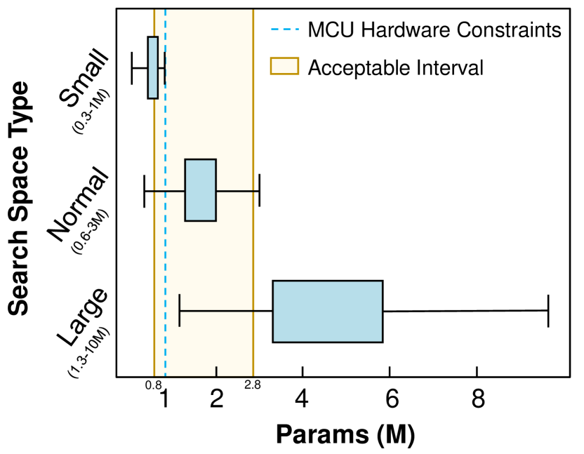
(a)

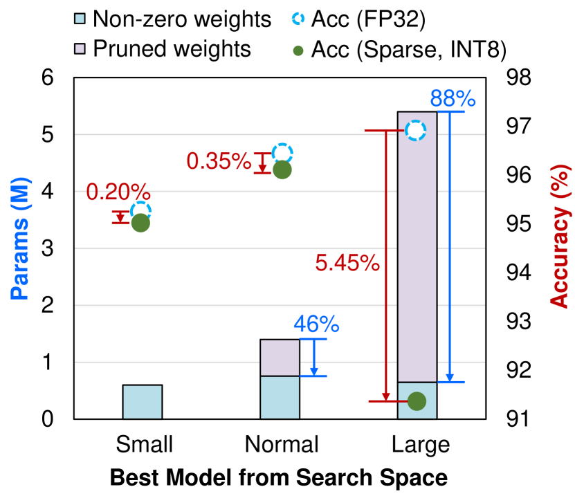
(b)

Figure 10: (a) The obtained model size from three types of search space. The model sampled from a small search space satisfies the hardware constraints without pruning. The models sampled from large search spaces require compression to meet the constraints. (b) The best-performing model in each search space.

TABLE II: Ablation of TinyFormer in offline evaluation. Basic TinyFormer structure has two DoTs and mixed block size. All the models are searched with hardware constraints of $300$KB Memory and $980$KB Storage in CIFAR-10, and each has $300$KB peak memory in the searching procedure. #Params indicate the number of effective weights.

Model	Accuracy	# Params	Storage
TinyFormer	$\boldsymbol{96.10\%}$	$731$K	$942$KB
TinyFormer (w/o Tr.)	$94.62\%$	-	$963$KB
TinyFormer (Single DoT)	$93.92\%$	-	$655$KB
TinyFormer (Block Size $=2$)	$95.88\%$	$730$K	$950$KB
TinyFormer (Block Size $=4$)	$95.52\%$	$807$K	$962$KB

The search space design usually affects the sampled model size. An inappropriate search space will have a negative impact on the experimental results. As shown in Fig. 10(a), we conduct experiments on three different sizes of search spaces, including small, normal and large. With hyper-parameter $\lambda_{lo}=0.8$ and $\lambda_{hi}=2.8$, only normal space has acceptance probability higher than $90\%$. The small and large space has acceptance probability less than $30\%$. The small search space mostly contains dense model with low capacity, while models in large search space have both higher parameter counts and higher sparsity. Fig. 10(b) shows the accuracy and compression ratio of the best model obtained from each search space. While the model searched from the small search space does not require pruning, the accuracy is inferior to others. The model searched from the large search space has the highest original accuracy. However, it needs to be cut down $88\%$ of weights to meet the hardware constraint, which leads to a significant accuracy drop. On the other hand, the model searched from normal search space has a good balance between the model size and sparsity, and achieves the highest accuracy on MCUs.

Ablation Study

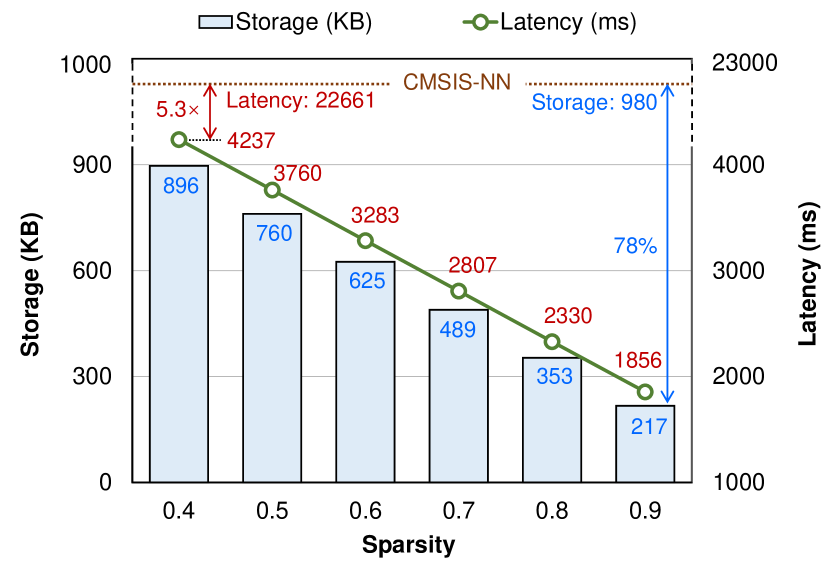
Figure 11: Performance comparis of SparseEngine and CMSIS-NN on CIFAR-10. SparseEngine is $5.3\times$$\sim$$12.2\times$ faster than CMSIS-NN under different sparsity, while saving $9\%$$\sim$$78\%$ storage.

In this part, we show the ablation study on TinyFormer from Table II, which consists of three perspectives: whether to use transformer block, number of DoTs, and whether to adopt mixed block size pruning in search stage. In Table II, TinyFormer refers to the TinyFormer-300K model adopted in Table I, with transformer block, two DoTs, and mixed block size pruning.

In order to understand the impact of transformer block in TinyFormer, a CNN model without transformer block is searched and denoted as TinyFormer (w/o Tr.). TinyFormer (w/o Tr.) deletes the transformer block in DoT architecture, and only remains the downsample block and MobileNetV2 block. Compared to TinyFormer (w/o Tr.), TinyFormer obtains better performance under almost the same resource usage, which also increases the accuracy by $1.5\%$. These results suggest that incorporating transformer-related blocks or layers can offer advantages in achieving improved performance for TinyML.

Additionally, we also conducted experiments to evaluate the impact of the number of DoT layers on model’s accuracy. TinyFormer (Single DoT) is derived from the supernet that exclusively consists of a single DoT architecture, while adhering to the same hardware constraints. In terms of storage occupation, TinyFormer (Single DoT) utilizes only $66.8\%$ of the storage limitation, resulting in a decrease in accuracy by $1.48\%$. When employing a single DoT, the main bottleneck for TinyFormer (Single DoT) arises from memory constraints. In contrast, the model with two DoTs almost approaches the limits of both storage and memory, effectively maximizing resources utilization. Therefore, two DoTs are utilized in our basic experiments.

Finally, we evaluate the effectiveness of the mixed block size strategy in two stages of SparseNAS. In particular, TinyFormer (Block Size $=2$) and TinyFormer (Block Size $=4$) denote models with a fixed block size of $2$ and $4$, respectively, in block pruning. Table II demonstrates that larger block sizes allow for more efficient storage of weights within the given limitations. However, setting all block sizes to $4$ adversely affects model’s accuracy. Based on these results, the pruning method employing a mixed block size scheme strikes the best balance between block size and the number of effective weights, thereby yielding the most suitable model with optimal performance.

IV-C Runtime Evaluation

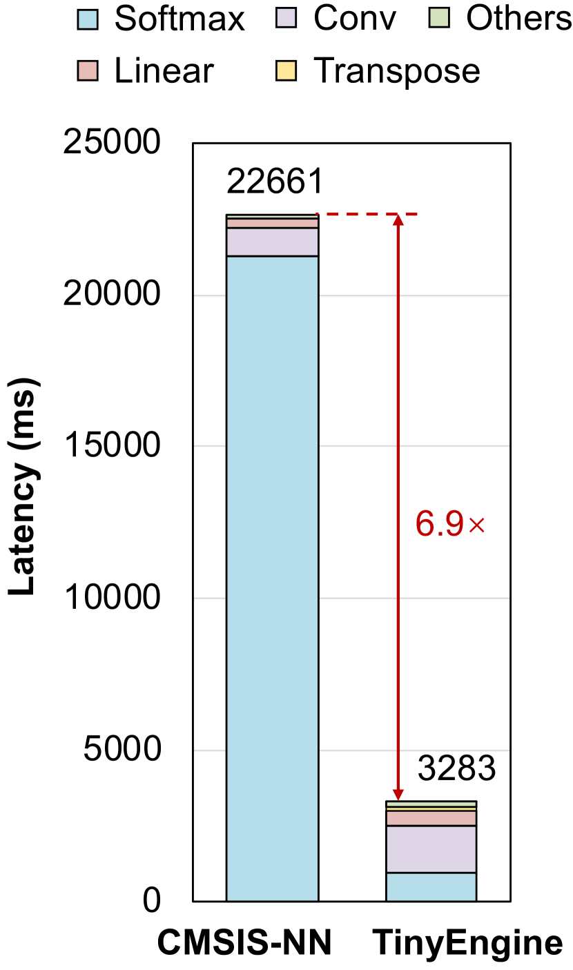
(a)

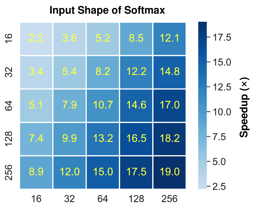
(b)

Figure 12: (a) In CMSIS-NN, Softmax operator occupies $94\%$ of the latency. SparseEngine optimizes the procedure of Softmax to achieve $6.9\times$ acceleration with $60\%$ sparsity. (b) Softmax acceleration in various input size between SparseEngine and CMSIS-NN.

TABLE III: Scaled-LayerNorm acceleration compared with normal LayerNorm. Most of experimental configurations are similar to TinyFormer-300K in Table I except for the LayerNorm implementations. The default normal LayerNorm is calculated with FP32 format.

Method	Accuracy	Shape	Latency
LayerNorm	$96.11\%$	$[256\times 44]$	$194$ms
		$[64\times 192]$	$208$ms
Scaled-LayerNorm	$96.10\%$	$[256\times 44]$	$5$ms
		$[64\times 192]$	$4$ms

At the runtime level, we have developed SparseEngine specifically for performing sparse inference on MCUs. The implementation of SparseEngine has successfully reduced the inference time to $3.8$ seconds on our highest-accuracy searched model. To evaluate the performance of SparseEngine, we deploy the same sparse model in both CMSIS-NN and SparseEngine. As illustrated in Fig. 11, SparseEngine outperforms CMSIS-NN both in terms of inference latency and storage occupation. By leveraging sparse inference support, SparseEngine achieves a significant reduction in storage requirements on MCUs, ranging from $9\%$ to $78\%$. Additionally, through the utilization of specialized optimizations, SparseEngine achieves an impressive acceleration of inference, ranging from $5.3\times$ to $12.2\times$. It is worth noting that in order to make a fair comparison with CMSIS-NN, we need to ensure that the model fits within the resource constraints in its dense form. Consequently, the model evaluated in this particular experiments can not achieve the highest accuracy.

To identify the bottleneck in the inference process, we evaluate the runtime breakdown for different layers. As depicted in Fig. 12(a), our findings indicate that the Softmax operator is responsible for the majority of the inference time. Within the Softmax operator, the most time-consuming step is the negative exponential calculation. However, we discovered that as the input size increases, the results of the negative exponential can be reused. Leveraging this observation, SparseEngine employs a bitmap lookup table to reduce redundant calculations and optimize the Softmax operator. Fig. 12(b) provides a comparison of the inference time for the Softmax operator between CMSIS-NN and SparseEngine, considering various input sizes. Notably, as the input size increases, SparseEngine exhibits more efficient optimization. In fact, with an input shape of $[256\times 256]$, SparseEngine achieves a speedup of up to $19\times$ for the Softmax operator.

Additionally, we also conducted an experiment involving Scaled-LayerNorm in TinyFormer. Our Scaled-LayerNorm performs integer-arithmetic calculations instead of previous normal LayerNorm operation, making it more suitable for model inference on MCUs. Furthermore, Scaled-LayerNorm addresses the issue of precision loss in quantization by expanding the range of normalization results during the rounding operation. Table III illustrates the impact of Scaled-LayerNorm on acceleration. Remarkably, the accuracy of TinyFormer using Scaled-LayerNorm is nearly equivalent to that of the normal LayerNorm computed in FP32 format, while the inference procedure is accelerated by a factor of $38.8\times$ to $52.0\times$. These experimental results align with our expectations, as Scaled-LayerNorm significantly enhances the efficiency of LayerNorm inference without any noticeable loss in accuracy. In summary, the experimental results for both Softmax and Scaled-LayerNorm validate our observations and highlight the substantial acceleration effects achieved by SparseEngine.

V Conclusions

In this work, TinyFormer is proposed as an innovative framework for developing efficient transformers on MCUs by integrating SuperNAS, SparseNAS and SparseEngine. One notable feature of TinyFormer is its ability to produce sparse models with high accuracy while adhering to hardware constraints. By integrating models sparsity and neural architecture search, TinyFormer achieves a delicate balance between efficiency and performance. Along with the automated deployment approaches, TinyFormer could further accomplish efficient sparse inference with a guaranteed latency on targeted MCUs. Experimental results demonstrate that TinyFormer could achieve $96.1\%$ accuracy on CIFAR-10 under the limitations of $1$MB storage and $320$KB memory. Compared with CMSIS-NN, TinyFormer achieves a remarkable speedup of up to $12.2\times$ and reduces storage requirements by up to $78\%$. These achievements not only bring powerful transformers into TinyML scenarios but also greatly expand the scope of deep learning applications.

Jianlei Yang (S’11-M’14-SM’20) received the B.S. degree in microelectronics from Xidian University, Xi’an, China, in 2009, and the Ph.D. degree in computer science and technology from Tsinghua University, Beijing, China, in 2014. He is currently an Associate Professor in Beihang University, Beijing, China, with the School of Computer Science and Engineering. From 2014 to 2016, he was a post-doctoral researcher with the Department of ECE, University of Pittsburgh, Pennsylvania, USA. His current research interests include deep learning accelerators and neuromorphic computing systems. Dr. Yang was the recipient of the First/Second place on ACM TAU Power Grid Simulation Contest in 2011/2012. He was a recipient of IEEE ICCD Best Paper Award in 2013, ACM GLSVLSI Best Paper Nomination in 2015, IEEE ICESS Best Paper Award in 2017, ACM SIGKDD Best Student Paper Award in 2020.

Jiacheng Liao received the B.S. degree in Computer Science and Technology from Beihang University, Beijing, China, in 2022. He is currently working toward the M.S. degree in Computer Science and Technology in Beihang University, Beijing, China. His current research interests include TinyML and ML systems.

Fanding Lei received the B.S. degree in Information and Electronics from Beijing Institute of Technology, Beijing, China, in 2020, and M.S. degree in Computer Science and Technology in Beihang University, Beijing, China, in 2022. His current research interests include TinyML and ML systems.

Meichen Liu received the B.S. degree in Computer Science and Technology from Beihang University, Beijing, China, in 2021. She is currently working toward the M.S. degree in Computer Science and Technology in Beihang University, Beijing, China. Her current research interests include TinyML and ML systems.

Junyi Chen is currently working toward the B.S. degree in Computer Science and Technology in Beihang University, Beijing, China. His current research interests include TinyML and ML systems.

Lingkun Long is currently working toward the B.S. degree in Computer Science and Technology in Beihang University, Beijing, China. His current research interests include TinyML and ML systems.

Han Wan received the B.S. degree and Ph.D. degree in Computer Science and Technology from Beihang University, Beijing, China, in 2003 and 2011, respectively. She is currently an Associate Professor with the School of Computer Science and Engineering at Beihang University. From 2015 to 2016, she was a visiting scholar with the Education Research Group, Massachusetts Institute of Technology (MIT). Her research interests include computer architectures and systems, educational data mining.

Bei Yu (M’15-SM’22) received the Ph.D. degree from The University of Texas at Austin in 2014. He is currently an Associate Professor in the Department of Computer Science and Engineering, The Chinese University of Hong Kong. He has served as TPC Chair of ACM/IEEE Workshop on Machine Learning for CAD, and in many journal editorial boards and conference committees. He is Editor of IEEE TCCPS Newsletter. He received nine Best Paper Awards from DATE 2022, ICCAD 2021 & 2013, ASPDAC 2021 & 2012, ICTAI 2019, Integration, the VLSI Journal in 2018, ISPD 2017, SPIE Advanced Lithography Conference 2016, and six ICCAD/ISPD contest awards.

Weisheng Zhao (Fellow, IEEE) received the Ph.D. degree in physics from the University of Paris Sud, Paris, France, in 2007. He is currently a Professor with the School of Integrated Circuit Science and Engineering, Beihang University, Beijing, China. In 2009, he joined the French National Research Center, Paris, as a Tenured Research Scientist. Since 2014, he has been a Distinguished Professor with Beihang University. He has published more than 200 scientific articles in leading journals and conferences, such as Nature Electronics, Nature Communications, Advanced Materials, IEEE Transactions, ISCA, and DAC. His current research interests include the hybrid integration of nanodevices with CMOS circuit and new nonvolatile memory (40-nm technology node and below) like MRAM circuit and architecture design. Prof. Zhao is currently the Editor-in-Chief for the IEEE Transactions on Circuits and System I: Regular Paper.

References

- [1] M. Shafique, T. Theocharides, V. J. Reddy, and B. Murmann, “TinyML: current progress, research challenges, and future roadmap,” in Proceedings of 58th ACM/IEEE Design Automation Conference (DAC), 2021, pp. 1303–1306.
- [2] Y. Zhang, N. Suda, L. Lai, and V. Chandra, “Hello Edge: Keyword spotting on microcontrollers,” arXiv preprint arXiv:1711.07128, 2017.
- [3] R. Kallimani, K. Pai, P. Raghuwanshi, S. Iyer, and O. L. López, “TinyML: Tools, Applications, Challenges, and Future Research Directions,” arXiv preprint arXiv:2303.13569, 2023.
- [4] C. R. Banbury, V. J. Reddi, M. Lam, W. Fu, A. Fazel, J. Holleman, X. Huang, R. Hurtado, D. Kanter, A. Lokhmotov et al., “Benchmarking TinyML systems: Challenges and direction,” arXiv preprint arXiv:2003.04821, 2020.
- [5] C. Banbury, C. Zhou, I. Fedorov, R. Matas, U. Thakker, D. Gope, V. Janapa Reddi, M. Mattina, and P. Whatmough, “MicroNets: Neural network architectures for deploying tinyml applications on commodity microcontrollers,” in Proceedings of Machine Learning and Systems (MLSys), 2021, pp. 517–532.
- [6] K. He, X. Zhang, S. Ren, and J. Sun, “Deep Residual Learning for Image Recognition,” in Proceedings of Conference on Computer Vision and Pattern Recognition (CVPR), 2016.
- [7] A. Vaswani, N. Shazeer, N. Parmar, J. Uszkoreit, L. Jones, A. N. Gomez, L. Kaiser, and I. Polosukhin, “Attention is All You Need,” in Proceedings of Advances in Neural Information Processing Systems (NeurIPS), 2017, pp. 5998–6008.
- [8] A. Gulati, J. Qin, C. Chiu, N. Parmar, Y. Zhang, J. Yu, W. Han, S. Wang, Z. Zhang, Y. Wu, and R. Pang, “Conformer: Convolution-augmented Transformer for Speech Recognition,” in Proceedings of 21st Annual Conference of the International Speech Communication Association (INTERSPEECH), 2020, pp. 5036–5040.
- [9] A. Dosovitskiy, L. Beyer, A. Kolesnikov, D. Weissenborn, X. Zhai, U. Thomas, M. Dehghani, M. Minderer, H. Georg, S. Gelly, U. Jakob, and H. Neil, “An Image is Worth 1616 Words: Transformers for Image Recognition at Scale,” in Proceedings of 9th International Conference on Learning Representations (ICLR), 2021.
- [10] S. Mehta and M. Rastegari, “MobileViT: Light-weight, General-purpose, and Mobile-friendly Vision Transformer,” in Proceedings of 10th International Conference on Learning Representations (ICLR), 2022.
- [11] H. Zhang, W. Hu, and X. Wang, “EdgeFormer: Improving Light-weight ConvNets by Learning from Vision Transformers,” arXiv preprint arXiv:2203.03952, 2022.
- [12] A. Hassani, S. Walton, N. Shah, A. Abuduweili, J. Li, and H. Shi, “Escaping the Big Data Paradigm with Compact Transformers,” arXiv preprint arXiv:2104.05704, 2021.
- [13] L. Lai, N. Suda, and V. Chandra, “CMSIS-NN: Efficient Neural Network Kernels for Arm Cortex-M CPUs,” arXiv preprint arXiv:1801.06601, 2018.
- [14] M. Rusci, A. Capotondi, and L. Benini, “Memory-Driven Mixed Low Precision Quantization For Enabling Deep Network Inference On Microcontrollers,” in Proceedings of Machine Learning and Systems (MLSys), 2020.
- [15] M. Rusci, M. Fariselli, A. Capotondi, and L. Benini, “Leveraging automated mixed-low-precision quantization for tiny edge microcontrollers,” IoT Streams for Data-Driven Predictive Maintenance and IoT, Edge, and Mobile for Embedded Machine Learning, vol. 1325, pp. 296–308, 2020.
- [16] M. Sandler, A. Howard, M. Zhu, A. Zhmoginov, and L.-C. Chen, “MobileNetV2: Inverted Residuals and Linear Bottlenecks,” in Proceedings of IEEE Conference on Computer Vision and Pattern Recognition (CVPR), 2018, pp. 4510–4520.
- [17] B. Zoph and Q. V. Le, “Neural Architecture Search with Reinforcement Learning,” in Proceedings of International Conference on Learning Representations (ICLR), 2017.
- [18] A. Zhou, J. Yang, Y. Qi, Y. Shi, T. Qiao, W. Zhao, and C. Hu, “Hardware-Aware Graph Neural Network Automated Design for Edge Computing Platforms,” in Proceedings of 60th ACM/IEEE Design Automation Conference (DAC), 2023.
- [19] B. Wu, X. Dai, P. Zhang, Y. Wang, F. Sun, Y. Wu, Y. Tian, P. Vajda, Y. Jia, and K. Keutzer, “FBNet: Hardware-Aware Efficient ConvNet Design via Differentiable Neural Architecture Search,” in Proceedings of IEEE Conference on Computer Vision and Pattern Recognition (CVPR), 2019, pp. 10 734–10 742.
- [20] H. Cai, L. Zhu, and S. Han, “ProxylessNAS: Direct neural architecture search on target task and hardware,” in Proceedings of 7th International Conference on Learning Representations (ICLR), 2019.
- [21] W. Jiang, L. Yang, E. H. Sha, Q. Zhuge, S. Gu, S. Dasgupta, Y. Shi, and J. Hu, “Hardware/software co-exploration of neural architectures,” IEEE Transactions on Computer-Aided Design of Integrated Circuits and Systems (TCAD), vol. 39, no. 12, pp. 4805–4815, 2020.
- [22] X. Luo, D. Liu, H. Kong, S. Huai, H. Chen, and W. Liu, “LightNAS: On lightweight and scalable neural architecture search for embedded platforms,” IEEE Transactions on Computer-Aided Design of Integrated Circuits and Systems (TCAD), vol. 42, no. 6, pp. 1784–1797, 2023.
- [23] I. Fedorov, R. P. Adams, M. Mattina, and P. Whatmough, “SpArSe: Sparse architecture search for CNNs on resource-constrained microcontrollers,” in Proceedings of Advances in Neural Information Processing Systems (NeurIPS), 2019, pp. 4978–4990.
- [24] M. Abadi, P. Barham, J. Chen, Z. Chen, A. Davis, J. Dean, M. Devin, S. Ghemawat, G. Irving, M. Isard, M. Kudlu, J. Levenberg, R. Monga, S. Moore, D. G.Murray, B. Steiner, P. Tucker, V. Vasudevan, P. Warden, M. Wicke, Y. Yu, and X. Zhang, “TensorFlow: A system for large-scale machine learning,” in Proceedings of 12th USENIX Symposium on Operating Systems Design and Implementation (OSDI), 2016, pp. 265–283.
- [25] T. Chen, T. Moreau, Z. Jiang, L. Zheng, E. Yan, M. Cowan, H. Shen, L. Wang, Y. Hu, L. Ceze, C. Guestrin, and A. Krishnamurthy, “TVM: An Automated End-to-End Optimizing Compiler for Deep Learning,” in Proceedings of 13th USENIX Symposium on Operating Systems Design and Implementation (OSDI), 2018, pp. 578–594.
- [26] A. Capotondi, M. Rusci, M. Fariselli, and L. Benini, “CMix-NN: Mixed low-precision CNN library for memory-constrained edge devices,” IEEE Transactions on Circuits and Systems II (TCAS-II), pp. 871–875, 2020.
- [27] J. Lin, W.-M. Chen, Y. Lin, C. John, C. Gan, and S. Han, “MCUNet: tiny deep learning on IoT devices,” in Proceedings of Advances in Neural Information Processing Systems (NeurIPS), 2020, pp. 11 711–11 722.
- [28] Z. Guo, X. Zhang, H. Mu, W. Heng, Z. Liu, Y. Wei, and J. Sun, “Single path one-shot neural architecture search with uniform sampling,” in Proceedings of 16th European Conference on Computer Vision (ECCV), vol. 12361, 2020, pp. 544–560.
- [29] A. F. Agarap, “Deep learning using rectified linear units (ReLU),” arXiv preprint arXiv:1803.08375, 2018.
- [30] M. Zhu and S. Gupta, “To prune, or not to prune: exploring the efficacy of pruning for model compression,” in Proceedings of 6th International Conference on Learning Representations (ICLR), 2018.
- [31] R. Krishnamoorthi, “Quantizing deep convolutional networks for efficient inference: A whitepaper,” arXiv preprint arXiv:1806.08342, 2018.
- [32] J. Yang, W. Fu, X. Cheng, X. Ye, P. Dai, and W. Zhao, “S2Engine: A novel systolic architecture for sparse convolutional neural networks,” IEEE Transactions on Computers (TC), vol. 71, no. 6, pp. 1440–1452, 2021.
- [33] P. Dai, J. Yang, X. Ye, X. Cheng, J. Luo, L. Song, Y. Chen, and W. Zhao, “SparseTrain: Exploiting dataflow sparsity for efficient convolutional neural networks training,” in Proceedings of 57th ACM/IEEE Design Automation Conference (DAC), 2020, pp. 1–6.
- [34] A. Krizhevsky, G. Hinton et al., “Learning Multiple Layers of Features from Tiny Images,” 2009.
- [35] I. Loshchilov and F. Hutter, “Decoupled Weight Decay Regularization,” in Proceedings of 7th International Conference on Learning Representations (ICLR), 2019.
- [36] C. Szegedy, V. Vanhoucke, S. Ioffe, J. Shlens, and Z. Wojna, “Rethinking the Inception Architecture for Computer Vision,” in Proceedings of IEEE Conference on Computer Vision and Pattern Recognition (CVPR), 2016, pp. 2818–2826.
- [37] J. Deng, W. Dong, R. Socher, L.-J. Li, K. Li, and F.-F. Li, “ImageNet: A large-scale hierarchical image database,” in Proceedings of IEEE Conference on Computer Vision and Pattern Recognition (CVPR), 2009.