Ramsey properties of randomly perturbed hypergraphs

Abstract

Let $\tilde{K}_{t}$ denote the $3$-uniform linear clique of order $t$. Given an even integer $t\geq 4$, let $M$ denote the asymmetric maximal density of $\tilde{K}_{t}$ and $\tilde{K}_{t/2}$. We prove that there exists a constant $C>0$ such that, if $(H_{n})_{n\in\mathbb{N}}$ is any sequence of dense $3$-uniform hypergraphs and $p:=p(n)\geq Cn^{-1/M}$, then

$$\lim_{n\to\infty}\mathbb{P}[H_{n}\cup R_{n}\to(\tilde{K}_{t})_{2}]=1$$

holds, whenever $R_{n}\sim\mathbb{H}(n,p)$, where the latter denotes the binomial $3$-uniform random hypergraph distribution. We conjecture that this result uncovers the threshold for the property in question for $t\geq 6$.

The key tools of our proof are a new variant of the Strong Hypergraph Regularity Lemma along with a new Tuple Lemma accompanying it. Our variant incorporates both the strong and the weak hypergraph regularity lemmas into a single lemma; allowing for graph-like applications of the strong lemma to be carried out in $3$-uniform hypergraphs.

1 Introduction

Given a distribution $\mathcal{R}$ over all $n$-vertex hypergraphs, as well as an $n$-vertex hypergraph $H$, referred to as the seed hypergraph, unions of the form $H\cup R$ with $R\sim\mathcal{R}$ define a distribution over the super-hypergraphs of $H$, denoted by $H\cup\mathcal{R}$. The hypergraphs $\Gamma\sim H\cup\mathcal{R}$ are referred to as random perturbations of $H$. The study of the properties of randomly perturbed hypergraphs has received much attention of late. Thus far, two dominant strands of results in this avenue have emerged. One strand is the study of the thresholds for the emergence of various spanning and nearly-spanning configurations within such structures (see, e.g., [3, 4, 5, 6, 10, 11, 12, 13, 21, 32, 41, 42, 47]); the second strand pertains to their Turán, Ramsey and anti-Ramsey properties (see, e.g., [1, 2, 6, 7, 18, 19, 20, 43, 52]). Our result lies in the latter vein.

The first to study Ramsey properties of randomly perturbed graphs were Krivelevich, Sudakov, and Tetali [43]. They determined that $n^{-2/(t-1)}$ is the threshold for the asymmetric Ramsey property $G\cup\mathbb{G}(n,p)\to(K_{3},K_{t})$, whenever $G$ is an $n$-vertex graph of edge-density $d\in(0,1/2)$ independent of $n$. The classical Ramsey arrow-notation $\Gamma\to(K_{3},K_{t})$ denotes the property that any $2$-edge-colouring of $\Gamma$ yields a monochromatic copy of $K_{3}$ occurring in the first colour or a monochromatic copy of $K_{t}$ occurring in the second colour.

The problem, put forth in [43], of determining the threshold for the property $G\cup\mathbb{G}(n,p)\to(K_{s},K_{t})$, whenever $G$ is dense and $s,t\geq 4$, remained open for many years and was only recently (essentially) resolved by Das and Treglown [20] who proved that $n^{-1/m_{2}(K_{t},K_{\lceil s/2\rceil})}$ is the threshold for the property $G\cup\mathbb{G}(n,p)\to(K_{s},K_{t})$, where here $G$ is a dense $n$-vertex graph, $t\geq s\geq 5$, and $m_{2}(H,F)$ denotes the asymmetric maximal $2$-density of two graphs $H$ and $F$. Other values of $t$ and $s$ are considered in [20, Theorem 1.7]. Of these, the case $s=t=4$ stands out; the threshold for the property $G\cup\mathbb{G}(n,p)\to(K_{4})_{2}$ is known to (essentially) be $n^{-1/2}$ by [52, Theorem 1.8] and [20, Theorem 5(ii)].

The aforementioned Ramsey-type results for randomly perturbed dense graphs are formulated for $2$-edge-colourings only. This restriction is well-justified. Indeed, suppose that more than two colours are available. The colouring in which the seed is coloured using one colour and the random perturbation is coloured using all the remaining colours, reduces the problem to that of studying the Ramsey property at hand for truly random hypergraphs.

The results seen in [20, 43, 52], as well as our result, stated in Theorem 1.4, are affected by the well-established line of research [17, 28, 31, 33, 36, 38, 44, 45, 46, 48, 50, 51, 53, 54, 55, 56] determining the thresholds of symmetric and asymmetric Ramsey properties of random hypergraphs. For random graphs, the thresholds for symmetric Ramsey properties are well-understood [17, 28, 31, 45, 50, 51, 53, 54, 55, 56]; in fact, a complete characterisation of these exists, see, e.g., [31, Theorem 1]. Minor exceptions aside, the latter asserts that $n^{-1/m_{2}(F)}$ is the threshold for the property $\mathbb{G}(n,p)\to(F)_{r}$, where $m_{2}(F)$ denotes the maximal $2$-densityfootnote 1 of a prescribed graph $F$, and $r$, taken to be independent of $n$, denotes the number of colours available. The thresholds of asymmetric Ramsey properties in random graphs are the subject of the Kohayakawa-Kreuter conjecture [36, 38]. The $1$-statement stipulated by this conjecture has been verified in [48] and progress has been made with respect to the corresponding $0$-statement [31, 33, 44, 46].

Much less is known regarding the thresholds of Ramsey properties of random hypergraphs of uniformity at least 3, captured through the distribution $\mathbb{H}^{(k)}(n,p)$, referred to as the $k$-uniform binomial random hypergraph. Unlike the case of graphs, a complete characterisation for the thresholds of symmetric Ramsey properties of $\mathbb{H}^{(k)}(n,p)$ is unavailable (see [50, Theorem 3] for further details). The following general bound is due to Friedgut, Rödl, and the third author.

Theorem 1.1.

[28] Let $r,k\geq 2$ be integers and let $F$ be a $k$-uniform hypergraph with maximum degree at least two. Then, there exists a constant $C>0$ such that $\mathbb{H}^{(k)}(n,p)\to(F)_{r}$ holds a.a.s. whenever $p:=p(n)\geq Cn^{-1/m_{k}(F)}$, where $m_{k}(F)$ denotes the maximal $k$-densityfootnote 1 of $F$.

Remark 1.2.

The lower bound on $p$, stated in Theorem 1.1, is in general best possible up to a constant factor. Indeed, if $F$ is complete, then $n^{-1/m_{k}(F)}$ is the threshold for the property $\mathbb{H}^{(k)}(n,p)\to(F)_{r}$ [28, 50].

Given the greater difficulty of studying Ramsey properties of hypergraphs, it is natural to consider special classes of hypergraphs. A hypergraph $H$ is said to be linear if $|e\cap f|\leq 1$ holds whenever $e,f\in E(H)$ are distinct. Linear hypergraphs are viewed as forming a certain middle ground between the realm of graphs and that of hypergraphs. A canonical example of linear hypergraphs exhibiting graph-like traits can be seen in the work [37] by Kohayakawa, Nagle, Rödl, and the third author, who proved that weak regularity suffices in order to support a counting lemma for any (fixed) linear hypergraph. In another vein, Füredi and Jiang [30] as well as Collier-Cartaino, Graber, and Jiang [14] determined the Turán density of linear cycles and the Turán density of linear trees was determined by Füredi [29].

Amongst the linear hypergraphs, linear cliques are of special interest. Given $t\geq 2$, the linear $3$-clique of order $t$, denoted $\tilde{K}_{t}$, is the $3$-uniform hypergraph with vertex-set $\left[t+\binom{t}{2}\right]$ and with positive minimum degree, where for every $1\leq i<j\leq t$ there is a unique $k>t$ such that $ijk$ forms an edge. This definition trivially extends to higher uniformities in which case we write $\tilde{K}^{(k)}_{t}$ to denote the linear $k$-clique of order $t$.

Over the years, linear cliques have attracted a lot of attention. Extending the classical theorem of Turán [59], Mubayi [49] determined the Turán density of linear cliques. The $2$-colour (symmetric) Ramsey number of $\tilde{K}_{t}$ grows polynomially in $t$ while its $4$-colour (symmetric) Ramsey number grows exponentially in $t$ [15]; that is, the Ramsey numbers of $\tilde{K}_{t}$ exhibit a strong dependence on the number of colours and as far as we know this is the sole family of hypergraphs known to have this trait (see [15] for further details).

1.1 Main results

For a $k$-uniform hypergraph ($k$-graph, hereafter) $H$, set

$$d_{k}(H):=\begin{cases}0,&\text{if $e(H)=0$},\\ 1/k&\text{if $e(H)=1,v(H)=k$},\\ \frac{e(H)-1}{v(H)-k},&\text{otherwise.}\end{cases}$$

The maximal $k$-density of $H$ is given by $m_{k}(H):=\max_{F\subseteq H}d_{k}(F)$. For an integer $t\geq 2$, let $M_{t}=m_{3}(\tilde{K}_{t})$.

Let $\mathbb{H}(n,p)$ denote the distribution over the $n$-vertex $3$-graphs, each member of which is obtained by retaining every member of $\binom{[n]}{3}$ as an hyperedge independently at random with probability $p$.

Prior to stating the main result of this paper, we address the more basic problem of determining the threshold for the emergence of a linear $3$-clique in a randomly perturbed dense $3$-graph. For a hypergraph $H$, let

$$m(H):=\max\left\{\frac{e(F)}{v(F)}:F\subseteq H,v(F)\geq 1\right\}$$

denote the maximum sub-hypergraph density of $H$. For $t\geq 3$, set $m(t):=m(\tilde{K}_{t})$. Note that $\tilde{K}_{t}$ is balanced, that is,

$$m(t)=\frac{e(\tilde{K}_{t})}{v(\tilde{K}_{t})}=\frac{\binom{t}{2}}{t+\binom{t}{2}}.$$

Proposition 1.3.

Let $t\geq 4$ be an integer. Then,

1. $\lim_{n\to\infty}\mathbb{P}[\tilde{K}_{t}\subseteq H\cup\mathbb{H}(n,p)]=1$ whenever $H$ is a dense $3$-graph with vertex-set $[n]$ and $p\gg n^{-\frac{1}{m(\lceil t/3\rceil)}}$.

2. there exists a dense $3$-graph $H_{0}$ with vertex-set $[n]$ such that $\lim_{n\to\infty}\mathbb{P}[\tilde{K}_{t}\subseteq H_{0}\cup\mathbb{H}(n,p)]=0$ whenever $p\ll n^{-\frac{1}{m(\lceil t/3\rceil)}}$.

The proof of Proposition 1.3 is deferred to Appendix A.

Given two $k$-graphs $H_{1}$ and $H_{2}$, each with at least one edge and such that $m_{k}(H_{1})\geq m_{k}(H_{2})$, the asymmetric maximal $k$-density of $H_{1}$ and $H_{2}$ is given by

$$m_{k}(H_{1},H_{2})=m_{k}(H_{2},H_{1}):=\max\left\{\frac{e(F)}{v(F)-k+1/m_{k}(H_{2})}:F\subseteq H_{1},e(F)\geq 1\right\}.$$ (1.1)

For integers $t_{1},t_{2}\geq 2$, let $M_{t_{1},t_{2}}=M_{t_{2},t_{1}}=m_{3}\left(\tilde{K}_{t_{1}},\tilde{K}_{t_{2}}\right)$.

Extending the results of [20, 43, 52] into the realm of hypergraphs, our main result, namely Theorem 1.4, concerning the emergence of monochromatic linear $3$-cliques in edge-coloured randomly perturbed dense $3$-graphs reads as follows.

Theorem 1.4.

For every $d>0$ and every even integer $t\geq 4$, there exists a constant $C>0$ such that

$$\lim_{n\to\infty}\mathbb{P}\left[H\cup\mathbb{H}(n,p)\to(\tilde{K}_{t})_{2}\right]=1$$

whenever $p:=p(n)\geq Cn^{-\frac{1}{M_{t,t/2}}}$ and $H$ is a $3$-graph with vertex-set $[n]$ and $e(H)\geq dn^{3}$.

Remark 1.5.

Our proof of Theorem 1.4 can be adapted so as to produce results of similar spirit for the asymmetric Ramsey property $H\cup\mathbb{H}(n,p)\to(\tilde{K}^{(k)}_{s},\tilde{K}^{(k)}_{t})$ for a wide range of values of $s$ and $t$, whenever $H$ is a dense $k$-graph for some $k\geq 3$. In particular, the restrictions to uniformity $3$ and $t$ being even are for convenience only. We do not pursue these extensions in this paper.

We conjecture that Theorem 1.4 uncovers the threshold for the Ramsey property in question; see Conjecture 7.5.

Our proof of Theorem 1.4 relies on two additional new results; their formal statements are postponed until Section 3 due to their highly technical nature. Roughly put, we prove a new variant of the so-called Strong Hypergraph Regularity Lemma (Strong Lemma, hereafter) established by Rödl and the third author [57]. The main addition of our variant, seen in Lemma 3.1, is that it offers a regularity lemma for ($3$-uniform) hypergraphs incorporating both the original Strong Lemma, namely Lemma 2.6, and the Weak Hypergraph Regularity Lemma (Weak Lemma, hereafter), namely Lemma 2.5, in such a way that the weak-regularity thresholds coincide with that seen for the triadsfootnote 2 forming the strong-regularity structure. A ‘hybrid’ hypergraph regularity lemma of a similar spirit can be seen in [8] as well; the latter, though, is insufficient for our needs. In Section 5, following the statement of our variant of the Strong Lemma, we address the variant seen in [8] with more detail and compare it with our formulation.

For certain applications, this combination between the ease of use of the Weak Lemma and the heightened control offered by its strong counterpart allows one to operate with the new variant of the Strong Lemma in a graph-like fashion within the context of $3$-uniform hypergraphs. Our proof of Theorem 1.4, presented in Section 4.2, is a demonstration of this assertion.

Various limitations accompany the Weak Lemma; these detract from its ease of use. A key feature accompanying the Graph Regularity Lemma [39, 40, 58] is the useful so-called tuple property (also referred to as the intersection property) stated in Lemma 3.4 below. Such a property is missing in weakly-regular hypergraphsfootnote 2. For our second main (technical) result, we endow the original Strong Lemma with an appropriate tuple property captured in Lemma 3.5. Operating this last lemma within the framework of our new variant of the Strong Lemma is akin to equipping the Weak Lemma with a much needed tuple property.

Organisation. In Section 2, we collect definitions, notation, and results pertaining to the regularity method. In Section 3, we state our main technical results, namely Lemmas 3.1 and 3.5. In Section 4, we prove Theorem 1.4. In Section 5, we prove our new variant of the Strong Lemma, namely Lemma 3.1. Finally, in Section 6, we prove Lemma 3.5, the aforementioned tuple property for the Strong Lemma.

2 Preliminaries

Let $V$ be a finite set. A partition $\mathcal{U}$ of $V$ given by $V=U_{1}\mathbin{\mathchoice{\leavevmode\vtop{\halign{\hfil$\m@th\displaystyle#$\hfil\cr\cup\cr\cdot\crcr}}}{\leavevmode\vtop{\halign{\hfil$\m@th\textstyle#$\hfil\cr\cup\cr\cdot\crcr}}}{\leavevmode\vtop{\halign{\hfil$\m@th\scriptstyle#$\hfil\cr\cup\cr\cdot\crcr}}}{\leavevmode\vtop{\halign{\hfil$\m@th\scriptscriptstyle#$\hfil\cr\cup\cr\cdot\crcr}}}}\cdots\mathbin{\mathchoice{\leavevmode\vtop{\halign{\hfil$\m@th\displaystyle#$\hfil\cr\cup\cr\cdot\crcr}}}{\leavevmode\vtop{\halign{\hfil$\m@th\textstyle#$\hfil\cr\cup\cr\cdot\crcr}}}{\leavevmode\vtop{\halign{\hfil$\m@th\scriptstyle#$\hfil\cr\cup\cr\cdot\crcr}}}{\leavevmode\vtop{\halign{\hfil$\m@th\scriptscriptstyle#$\hfil\cr\cup\cr\cdot\crcr}}}}U_{r}$ is said to be equitable if $|U_{1}|\leq|U_{2}|\leq\cdots\leq|U_{r}|\leq|U_{1}|+1$. Given an additional partition of $V$, namely $\mathcal{V}$, of the form $V=V_{1}\mathbin{\mathchoice{\leavevmode\vtop{\halign{\hfil$\m@th\displaystyle#$\hfil\cr\cup\cr\cdot\crcr}}}{\leavevmode\vtop{\halign{\hfil$\m@th\textstyle#$\hfil\cr\cup\cr\cdot\crcr}}}{\leavevmode\vtop{\halign{\hfil$\m@th\scriptstyle#$\hfil\cr\cup\cr\cdot\crcr}}}{\leavevmode\vtop{\halign{\hfil$\m@th\scriptscriptstyle#$\hfil\cr\cup\cr\cdot\crcr}}}}\cdots\mathbin{\mathchoice{\leavevmode\vtop{\halign{\hfil$\m@th\displaystyle#$\hfil\cr\cup\cr\cdot\crcr}}}{\leavevmode\vtop{\halign{\hfil$\m@th\textstyle#$\hfil\cr\cup\cr\cdot\crcr}}}{\leavevmode\vtop{\halign{\hfil$\m@th\scriptstyle#$\hfil\cr\cup\cr\cdot\crcr}}}{\leavevmode\vtop{\halign{\hfil$\m@th\scriptscriptstyle#$\hfil\cr\cup\cr\cdot\crcr}}}}V_{\ell}$, we say that $\mathcal{V}$ refines $\mathcal{U}$, and write $\mathcal{V}\prec\mathcal{U}$, if for every $i\in[\ell]$ there exists some $j\in[r]$ such that $V_{i}\subseteq U_{j}$ holds. For $k\geq 2$, write $K^{(k)}(\mathcal{U})$ to denote the complete $|\mathcal{U}|$-partite $k$-graph whose vertex-set is $V$ and whose edge-set is given by all members of $\binom{V}{k}$ meeting every member of $\mathcal{U}$ (termed cluster hereafter) in at most one vertex. If $\mathcal{U}=\{U,U^{\prime}\}$ consists of only two clusters, then we abbreviate $K^{(2)}(\mathcal{U})$ to $K^{(2)}(U,U^{\prime})$. In addition, we write $K^{(2)}(V)$ to denote the complete graph whose vertex-set is $V$.

2.1 Graph regularity

Let $d,\delta>0$ be given. A bipartite $2$-graph $G=(X\mathbin{\mathchoice{\leavevmode\vtop{\halign{\hfil$\m@th\displaystyle#$\hfil\cr\cup\cr\cdot\crcr}}}{\leavevmode\vtop{\halign{\hfil$\m@th\textstyle#$\hfil\cr\cup\cr\cdot\crcr}}}{\leavevmode\vtop{\halign{\hfil$\m@th\scriptstyle#$\hfil\cr\cup\cr\cdot\crcr}}}{\leavevmode\vtop{\halign{\hfil$\m@th\scriptscriptstyle#$\hfil\cr\cup\cr\cdot\crcr}}}}Y,E)$ is said to be $(\delta,d)$-regular if

$$e_{G}(X^{\prime},Y^{\prime})=d|X^{\prime}||Y^{\prime}|\pm\delta|X||Y|$$

holds for every $X^{\prime}\subseteq X$ and $Y^{\prime}\subseteq Y$. If $d$ coincides with the edge-density of $G$, i.e. $d=\frac{e(G)}{|X||Y|}$, then we abbreviate $(\delta,d)$-regular to $\delta$-regular. A tripartite $2$-graph $P$ with vertex-set $V(P)=X\mathbin{\mathchoice{\leavevmode\vtop{\halign{\hfil$\m@th\displaystyle#$\hfil\cr\cup\cr\cdot\crcr}}}{\leavevmode\vtop{\halign{\hfil$\m@th\textstyle#$\hfil\cr\cup\cr\cdot\crcr}}}{\leavevmode\vtop{\halign{\hfil$\m@th\scriptstyle#$\hfil\cr\cup\cr\cdot\crcr}}}{\leavevmode\vtop{\halign{\hfil$\m@th\scriptscriptstyle#$\hfil\cr\cup\cr\cdot\crcr}}}}Y\mathbin{\mathchoice{\leavevmode\vtop{\halign{\hfil$\m@th\displaystyle#$\hfil\cr\cup\cr\cdot\crcr}}}{\leavevmode\vtop{\halign{\hfil$\m@th\textstyle#$\hfil\cr\cup\cr\cdot\crcr}}}{\leavevmode\vtop{\halign{\hfil$\m@th\scriptstyle#$\hfil\cr\cup\cr\cdot\crcr}}}{\leavevmode\vtop{\halign{\hfil$\m@th\scriptscriptstyle#$\hfil\cr\cup\cr\cdot\crcr}}}}Z$ is said to be a $(\delta,d)$-triad, if $P[X,Y]$, $P[Y,Z]$, and $P[X,Z]$ are all $(\delta,d)$-regular. For a $2$-graph $G$, let $\mathcal{K}_{3}(G)$ denote the family of members of $\binom{V(G)}{3}$ spanning a triangle in $G$.

Lemma 2.1.

(The Triangle Counting Lemma [27, Fact A]) Let $d>0$, let $0<\delta<d/2$, and let $P$ be a $(\delta,d)$-triad with vertex-set $V(P)=X\mathbin{\mathchoice{\leavevmode\vtop{\halign{\hfil$\m@th\displaystyle#$\hfil\cr\cup\cr\cdot\crcr}}}{\leavevmode\vtop{\halign{\hfil$\m@th\textstyle#$\hfil\cr\cup\cr\cdot\crcr}}}{\leavevmode\vtop{\halign{\hfil$\m@th\scriptstyle#$\hfil\cr\cup\cr\cdot\crcr}}}{\leavevmode\vtop{\halign{\hfil$\m@th\scriptscriptstyle#$\hfil\cr\cup\cr\cdot\crcr}}}}Y\mathbin{\mathchoice{\leavevmode\vtop{\halign{\hfil$\m@th\displaystyle#$\hfil\cr\cup\cr\cdot\crcr}}}{\leavevmode\vtop{\halign{\hfil$\m@th\textstyle#$\hfil\cr\cup\cr\cdot\crcr}}}{\leavevmode\vtop{\halign{\hfil$\m@th\scriptstyle#$\hfil\cr\cup\cr\cdot\crcr}}}{\leavevmode\vtop{\halign{\hfil$\m@th\scriptscriptstyle#$\hfil\cr\cup\cr\cdot\crcr}}}}Z$. Then,

$$(1-2\delta)(d-\delta)^{3}|X||Y||Z|\leq|\mathcal{K}_{3}(P)|\leq((d+\delta)^{3}+2\delta)|X||Y||Z|.$$

In particular, if $d\leq 1/2$, then

$$|\mathcal{K}_{3}(P)|=(d^{3}\pm 4\delta)|X||Y||Z|$$ (2.1)

holds.

We shall also require the following less-known two-sided variant of the Triangle Counting Lemma; its proof is included for completeness.

Lemma 2.2.

(Two-Sided Triangle Counting Lemma) Let $P=(X\mathbin{\mathchoice{\leavevmode\vtop{\halign{\hfil$\m@th\displaystyle#$\hfil\cr\cup\cr\cdot\crcr}}}{\leavevmode\vtop{\halign{\hfil$\m@th\textstyle#$\hfil\cr\cup\cr\cdot\crcr}}}{\leavevmode\vtop{\halign{\hfil$\m@th\scriptstyle#$\hfil\cr\cup\cr\cdot\crcr}}}{\leavevmode\vtop{\halign{\hfil$\m@th\scriptscriptstyle#$\hfil\cr\cup\cr\cdot\crcr}}}}Y\mathbin{\mathchoice{\leavevmode\vtop{\halign{\hfil$\m@th\displaystyle#$\hfil\cr\cup\cr\cdot\crcr}}}{\leavevmode\vtop{\halign{\hfil$\m@th\textstyle#$\hfil\cr\cup\cr\cdot\crcr}}}{\leavevmode\vtop{\halign{\hfil$\m@th\scriptstyle#$\hfil\cr\cup\cr\cdot\crcr}}}{\leavevmode\vtop{\halign{\hfil$\m@th\scriptscriptstyle#$\hfil\cr\cup\cr\cdot\crcr}}}}Z,E_{P})$ be a tripartite $2$-graph such that $P[X,Y]$ and $P[X,Z]$ are both $(\delta,d)$-regular. In addition, let $X^{\prime}\subseteq X$ be a set of size $|X^{\prime}|\geq\delta|X|$. Then,

$$(d-\delta)d|X^{\prime}|e(P[Y,Z])-2\delta|X||Y||Z|\leq|\mathcal{K}_{3}(P,X^{\prime})|\leq(d+\delta)d|X^{\prime}|e(P[Y,Z])+2\delta|X||Y||Z|$$

holds, where $\mathcal{K}_{3}(P,X^{\prime})$ denotes the set of triangles of $P$ meeting $X^{\prime}$.

Proof.   Let $Y^{\prime}\subseteq Y$ consist of all vertices $y\in Y$ satisfying $\deg_{P}(y,X^{\prime})\geq(d-\delta)|X^{\prime}|$; note that $|Y^{\prime}|\geq(1-\delta)|Y|$ holds by Lemma 3.4 (see Section 3). We may then write

$$|\mathcal{K}_{3}(P,X^{\prime})| \geq\sum_{y\in Y^{\prime}}\Big{(}d(d-\delta)|X^{\prime}|\deg_{P}(y,Z)-\delta|X||Z|\Big{)}$$

$$=d(d-\delta)|X^{\prime}|\left(\sum_{y\in Y}\deg_{P}(y,Z)-\sum_{y\in Y\setminus Y^{\prime}}\deg_{P}(y,Z)\right)-\sum_{y\in Y^{\prime}}\delta|X||Z|$$

$$\geq d(d-\delta)|X^{\prime}|e(P[Y,Z])-d(d-\delta)\delta|X||Y||Z|-\delta|X||Y||Z|$$

$$\geq d(d-\delta)|X^{\prime}|e(P[Y,Z])-2\delta|X||Y||Z|.$$

Next, we prove the upper bound. Let $Y^{\prime\prime}\subseteq Y$ consist of all vertices $y\in Y$ satisfying $\deg_{P}(y,X^{\prime})\leq(d+\delta)|X^{\prime}|$; note that $|Y^{\prime\prime}|\geq(1-\delta)|Y|$ holds by Lemma 3.4. We may then write

$$|\mathcal{K}_{3}(P,X^{\prime})| \leq\sum_{y\in Y^{\prime\prime}}\Big{(}d(d+\delta)|X^{\prime}|\deg_{P}(y,Z)+\delta|X||Z|\Big{)}+\sum_{y\in Y\setminus Y^{\prime\prime}}|X^{\prime}||Z|$$

$$\leq d(d+\delta)|X^{\prime}|\left(\sum_{y\in Y}\deg_{P}(y,Z)-\sum_{y\in Y\setminus Y^{\prime\prime}}\deg_{P}(y,Z)\right)+\sum_{y\in Y^{\prime\prime}}\delta|X||Z|+\sum_{y\in Y\setminus Y^{\prime\prime}}|X||Z|$$

$$\leq d(d+\delta)|X^{\prime}|e(P[Y,Z])+2\delta|X||Y||Z|.$$

$\blacksquare$

The next lemma is commonly referred to as the Slicing Lemma (see, e.g., [40, Fact 1.5]).

Lemma 2.3.

(The Slicing Lemma) Let $d:=d_{\ref{lem:slicing}}$, let $\delta:=\delta_{\ref{lem:slicing}}>0$, and let $G:=(A\mathbin{\mathchoice{\leavevmode\vtop{\halign{\hfil$\m@th\displaystyle#$\hfil\cr\cup\cr\cdot\crcr}}}{\leavevmode\vtop{\halign{\hfil$\m@th\textstyle#$\hfil\cr\cup\cr\cdot\crcr}}}{\leavevmode\vtop{\halign{\hfil$\m@th\scriptstyle#$\hfil\cr\cup\cr\cdot\crcr}}}{\leavevmode\vtop{\halign{\hfil$\m@th\scriptscriptstyle#$\hfil\cr\cup\cr\cdot\crcr}}}}B,E)$ be a $(\delta,d)$-regular bipartite graph. Let $\delta\leq\alpha:=\alpha_{\ref{lem:slicing}}\leq 1$, and let $A^{\prime}\subseteq A$ and $B^{\prime}\subseteq B$ be sets of sizes $|A^{\prime}|\geq\alpha|A|$ and $|B^{\prime}|\geq\alpha|B|$. Then, $G[A^{\prime},B^{\prime}]$ is $(\delta^{\prime},d^{\prime})$-regular where $\delta^{\prime}=\max\{\delta/\alpha,2\delta\}$ and $d^{\prime}=d\pm\delta$.

The last ingredient related to graph regularity that is used in the sequel asserts that (bipartite) complements of regular pairs are themselves regular.

Observation 2.4.

If $G$ is a $(\delta,d)$-regular bipartite graph, then its (bipartite) complement is $(\delta,1-d)$-regular.

2.2 Hypergraph regularity

A direct generalisation of the notion of $\delta$-regularity, defined in the previous section for $2$-graphs, reads as follows. Let $d,\delta>0$. A tripartite $3$-graph $H:=(X\mathbin{\mathchoice{\leavevmode\vtop{\halign{\hfil$\m@th\displaystyle#$\hfil\cr\cup\cr\cdot\crcr}}}{\leavevmode\vtop{\halign{\hfil$\m@th\textstyle#$\hfil\cr\cup\cr\cdot\crcr}}}{\leavevmode\vtop{\halign{\hfil$\m@th\scriptstyle#$\hfil\cr\cup\cr\cdot\crcr}}}{\leavevmode\vtop{\halign{\hfil$\m@th\scriptscriptstyle#$\hfil\cr\cup\cr\cdot\crcr}}}}Y\mathbin{\mathchoice{\leavevmode\vtop{\halign{\hfil$\m@th\displaystyle#$\hfil\cr\cup\cr\cdot\crcr}}}{\leavevmode\vtop{\halign{\hfil$\m@th\textstyle#$\hfil\cr\cup\cr\cdot\crcr}}}{\leavevmode\vtop{\halign{\hfil$\m@th\scriptstyle#$\hfil\cr\cup\cr\cdot\crcr}}}{\leavevmode\vtop{\halign{\hfil$\m@th\scriptscriptstyle#$\hfil\cr\cup\cr\cdot\crcr}}}}Z,E)$ is said to be $(\delta,d)$-weakly-regular if

$$e_{H}(X^{\prime},Y^{\prime},Z^{\prime})=d|X^{\prime}||Y^{\prime}||Z^{\prime}|\pm\delta|X||Y||Z|$$

holds whenever $X^{\prime}\subseteq X$, $Y^{\prime}\subseteq Y$, and $Z^{\prime}\subseteq Z$. If $d=\frac{e(H)}{|X||Y||Z|}$, then we abbreviate $(\delta,d)$-weakly-regular to $\delta$-weakly-regular.

Given a partition $\mathcal{V}$ of a finite set $V$ defined by $V=V_{1}\mathbin{\mathchoice{\leavevmode\vtop{\halign{\hfil$\m@th\displaystyle#$\hfil\cr\cup\cr\cdot\crcr}}}{\leavevmode\vtop{\halign{\hfil$\m@th\textstyle#$\hfil\cr\cup\cr\cdot\crcr}}}{\leavevmode\vtop{\halign{\hfil$\m@th\scriptstyle#$\hfil\cr\cup\cr\cdot\crcr}}}{\leavevmode\vtop{\halign{\hfil$\m@th\scriptscriptstyle#$\hfil\cr\cup\cr\cdot\crcr}}}}\cdots\mathbin{\mathchoice{\leavevmode\vtop{\halign{\hfil$\m@th\displaystyle#$\hfil\cr\cup\cr\cdot\crcr}}}{\leavevmode\vtop{\halign{\hfil$\m@th\textstyle#$\hfil\cr\cup\cr\cdot\crcr}}}{\leavevmode\vtop{\halign{\hfil$\m@th\scriptstyle#$\hfil\cr\cup\cr\cdot\crcr}}}{\leavevmode\vtop{\halign{\hfil$\m@th\scriptscriptstyle#$\hfil\cr\cup\cr\cdot\crcr}}}}V_{t}$, a $3$-graph $H$ with $V(H)=V$ is said to be $\delta$-weakly-regular with respect to $\mathcal{V}$ if $H[X,Y,Z]$ is $\delta$-weakly-regular with respect to all but at most $\delta\binom{t}{3}$ triples $\{X,Y,Z\}\in\binom{\mathcal{V}}{3}$.

The following is a classical, straightforward and well-known adaptation of Szemerédi’s Graph Regularity Lemma [39, 40, 58].

Lemma 2.5.

(The weak $3$-graph regularity lemma) For every $\delta:=\delta_{\ref{lem:weak}}>0$ and positive integers $s:=s_{\ref{lem:weak}}$, $t:=t_{\ref{lem:weak}}$, and $h:=h_{\ref{lem:weak}}$ satisfying $t\geq h$, there exist positive integers $n_{0}$ and $T:=T_{\ref{lem:weak}}$ such that the following holds whenever $n\geq n_{0}$. Let $(H_{1},\ldots,H_{s})$ be a sequence of $n$-vertex $3$-graphs, all on the same vertex-set, namely $V$, and let $\mathcal{U}:=\mathcal{U}_{\ref{lem:weak}}$ be a vertex-partition of $V$ given by $V=U_{1}\mathbin{\mathchoice{\leavevmode\vtop{\halign{\hfil$\m@th\displaystyle#$\hfil\cr\cup\cr\cdot\crcr}}}{\leavevmode\vtop{\halign{\hfil$\m@th\textstyle#$\hfil\cr\cup\cr\cdot\crcr}}}{\leavevmode\vtop{\halign{\hfil$\m@th\scriptstyle#$\hfil\cr\cup\cr\cdot\crcr}}}{\leavevmode\vtop{\halign{\hfil$\m@th\scriptscriptstyle#$\hfil\cr\cup\cr\cdot\crcr}}}}\ldots\mathbin{\mathchoice{\leavevmode\vtop{\halign{\hfil$\m@th\displaystyle#$\hfil\cr\cup\cr\cdot\crcr}}}{\leavevmode\vtop{\halign{\hfil$\m@th\textstyle#$\hfil\cr\cup\cr\cdot\crcr}}}{\leavevmode\vtop{\halign{\hfil$\m@th\scriptstyle#$\hfil\cr\cup\cr\cdot\crcr}}}{\leavevmode\vtop{\halign{\hfil$\m@th\scriptscriptstyle#$\hfil\cr\cup\cr\cdot\crcr}}}}U_{h}$. Then, there exists an equitable vertex partition $\mathcal{V}$, given by $V=V_{1}\mathbin{\mathchoice{\leavevmode\vtop{\halign{\hfil$\m@th\displaystyle#$\hfil\cr\cup\cr\cdot\crcr}}}{\leavevmode\vtop{\halign{\hfil$\m@th\textstyle#$\hfil\cr\cup\cr\cdot\crcr}}}{\leavevmode\vtop{\halign{\hfil$\m@th\scriptstyle#$\hfil\cr\cup\cr\cdot\crcr}}}{\leavevmode\vtop{\halign{\hfil$\m@th\scriptscriptstyle#$\hfil\cr\cup\cr\cdot\crcr}}}}V_{2}\mathbin{\mathchoice{\leavevmode\vtop{\halign{\hfil$\m@th\displaystyle#$\hfil\cr\cup\cr\cdot\crcr}}}{\leavevmode\vtop{\halign{\hfil$\m@th\textstyle#$\hfil\cr\cup\cr\cdot\crcr}}}{\leavevmode\vtop{\halign{\hfil$\m@th\scriptstyle#$\hfil\cr\cup\cr\cdot\crcr}}}{\leavevmode\vtop{\halign{\hfil$\m@th\scriptscriptstyle#$\hfil\cr\cup\cr\cdot\crcr}}}}\cdots\mathbin{\mathchoice{\leavevmode\vtop{\halign{\hfil$\m@th\displaystyle#$\hfil\cr\cup\cr\cdot\crcr}}}{\leavevmode\vtop{\halign{\hfil$\m@th\textstyle#$\hfil\cr\cup\cr\cdot\crcr}}}{\leavevmode\vtop{\halign{\hfil$\m@th\scriptstyle#$\hfil\cr\cup\cr\cdot\crcr}}}{\leavevmode\vtop{\halign{\hfil$\m@th\scriptscriptstyle#$\hfil\cr\cup\cr\cdot\crcr}}}}V_{\tilde{t}}$, where $t\leq\tilde{t}\leq T$, such that $\mathcal{V}\prec\mathcal{U}$ and, moreover, $H_{i}$ is $\delta$-weakly-regular with respect to $\mathcal{V}$ for every $i\in[s]$.

We proceed to the statement of the Strong hypergraph Regularity Lemma for $3$-graphs following the formulation seen in [57]. Given a $2$-graph $G$, the relative density of a $3$-graph $H$ with vertex-set $V(H)=V(G)$, with respect to $G$ is given by

$$d(H|G):=\frac{|E(H)\cap\mathcal{K}_{3}(G)|}{|\mathcal{K}_{3}(G)|}.$$ (2.2)

For $\delta,d>0$ and a positive integer $r$, a tripartite $3$-graph $H=(X\mathbin{\mathchoice{\leavevmode\vtop{\halign{\hfil$\m@th\displaystyle#$\hfil\cr\cup\cr\cdot\crcr}}}{\leavevmode\vtop{\halign{\hfil$\m@th\textstyle#$\hfil\cr\cup\cr\cdot\crcr}}}{\leavevmode\vtop{\halign{\hfil$\m@th\scriptstyle#$\hfil\cr\cup\cr\cdot\crcr}}}{\leavevmode\vtop{\halign{\hfil$\m@th\scriptscriptstyle#$\hfil\cr\cup\cr\cdot\crcr}}}}Y\mathbin{\mathchoice{\leavevmode\vtop{\halign{\hfil$\m@th\displaystyle#$\hfil\cr\cup\cr\cdot\crcr}}}{\leavevmode\vtop{\halign{\hfil$\m@th\textstyle#$\hfil\cr\cup\cr\cdot\crcr}}}{\leavevmode\vtop{\halign{\hfil$\m@th\scriptstyle#$\hfil\cr\cup\cr\cdot\crcr}}}{\leavevmode\vtop{\halign{\hfil$\m@th\scriptscriptstyle#$\hfil\cr\cup\cr\cdot\crcr}}}}Z,E_{H})$ is said to be $(\delta,d,r)$-regular with respect to a tripartite $2$-graph $P=(X\mathbin{\mathchoice{\leavevmode\vtop{\halign{\hfil$\m@th\displaystyle#$\hfil\cr\cup\cr\cdot\crcr}}}{\leavevmode\vtop{\halign{\hfil$\m@th\textstyle#$\hfil\cr\cup\cr\cdot\crcr}}}{\leavevmode\vtop{\halign{\hfil$\m@th\scriptstyle#$\hfil\cr\cup\cr\cdot\crcr}}}{\leavevmode\vtop{\halign{\hfil$\m@th\scriptscriptstyle#$\hfil\cr\cup\cr\cdot\crcr}}}}Y\mathbin{\mathchoice{\leavevmode\vtop{\halign{\hfil$\m@th\displaystyle#$\hfil\cr\cup\cr\cdot\crcr}}}{\leavevmode\vtop{\halign{\hfil$\m@th\textstyle#$\hfil\cr\cup\cr\cdot\crcr}}}{\leavevmode\vtop{\halign{\hfil$\m@th\scriptstyle#$\hfil\cr\cup\cr\cdot\crcr}}}{\leavevmode\vtop{\halign{\hfil$\m@th\scriptscriptstyle#$\hfil\cr\cup\cr\cdot\crcr}}}}Z,E_{P})$ if

$$\left|\Big{|}\bigcup_{i=1}^{r}(E_{H}\cap\mathcal{K}_{3}(Q_{i}))\Big{|}-d\Big{|}\bigcup_{i=1}^{r}\mathcal{K}_{3}(Q_{i})\Big{|}\right|\leq\delta|\mathcal{K}_{3}(P)|$$ (2.3)

holds for every family of, not necessarily disjoint, subgraphs $Q_{1},\ldots,Q_{r}\subseteq P$ satisfying

$$\left|\bigcup_{i=1}^{r}\mathcal{K}_{3}(Q_{i})\right|\geq\delta\left|\mathcal{K}_{3}(P)\right|>0.$$

Let $V$ be a finite set and let $\mathcal{V}$ be a partition $V_{1}\mathbin{\mathchoice{\leavevmode\vtop{\halign{\hfil$\m@th\displaystyle#$\hfil\cr\cup\cr\cdot\crcr}}}{\leavevmode\vtop{\halign{\hfil$\m@th\textstyle#$\hfil\cr\cup\cr\cdot\crcr}}}{\leavevmode\vtop{\halign{\hfil$\m@th\scriptstyle#$\hfil\cr\cup\cr\cdot\crcr}}}{\leavevmode\vtop{\halign{\hfil$\m@th\scriptscriptstyle#$\hfil\cr\cup\cr\cdot\crcr}}}}\ldots\mathbin{\mathchoice{\leavevmode\vtop{\halign{\hfil$\m@th\displaystyle#$\hfil\cr\cup\cr\cdot\crcr}}}{\leavevmode\vtop{\halign{\hfil$\m@th\textstyle#$\hfil\cr\cup\cr\cdot\crcr}}}{\leavevmode\vtop{\halign{\hfil$\m@th\scriptstyle#$\hfil\cr\cup\cr\cdot\crcr}}}{\leavevmode\vtop{\halign{\hfil$\m@th\scriptscriptstyle#$\hfil\cr\cup\cr\cdot\crcr}}}}V_{h}$ of $V$, where $h$ is some positive integer. Given an integer $\ell\geq 1$, a partition $\mathcal{B}$ of $K^{(2)}(\mathcal{V})$ is said to be $\ell$-equitable with respect to $\mathcal{V}$ if it satisfies the following conditions:

(B.1)

every $B\in\mathcal{B}$ satisfies $B\subseteq K^{(2)}(V_{i},V_{j})$ for some distinct $i,j\in[h]$; and

(B.2)

for any distinct $i,j\in[h]$, precisely $\ell$ members of $\mathcal{B}$ partition $K^{(2)}(V_{i},V_{j})$.

We view partitions of $K^{(2)}(\mathcal{V})$ as partitions of $\binom{V}{2}$ under the agreement that the set $\{K^{(2)}(V_{i}):i\in[h]\}$ of complete graphs is added to the former; such an addition of cliques does not hinder the equitability notion defined in (B.2); it does violate (B.1), but this will not harm our arguments. Moreover, it is under this agreement that we say that a partition of $\binom{V}{2}$ refines a partition of $K^{(2)}(\mathcal{V})$.

For distinct indices $i,j\in[h]$, the partition of $K^{(2)}(V_{i},V_{j})$ induced by $\mathcal{B}$ is denoted by $\mathcal{B}^{ij}=\{B^{ij}_{\alpha}:=(V_{i}\mathbin{\mathchoice{\leavevmode\vtop{\halign{\hfil$\m@th\displaystyle#$\hfil\cr\cup\cr\cdot\crcr}}}{\leavevmode\vtop{\halign{\hfil$\m@th\textstyle#$\hfil\cr\cup\cr\cdot\crcr}}}{\leavevmode\vtop{\halign{\hfil$\m@th\scriptstyle#$\hfil\cr\cup\cr\cdot\crcr}}}{\leavevmode\vtop{\halign{\hfil$\m@th\scriptscriptstyle#$\hfil\cr\cup\cr\cdot\crcr}}}}V_{j},E^{ij}_{\alpha}):\alpha\in[\ell]\}$. The triads of $\mathcal{B}$ are the tripartite $2$-graphs having the form

$$B^{ijk}_{\alpha\beta\gamma}:=(V_{i}\mathbin{\mathchoice{\leavevmode\vtop{\halign{\hfil$\m@th\displaystyle#$\hfil\cr\cup\cr\cdot\crcr}}}{\leavevmode\vtop{\halign{\hfil$\m@th\textstyle#$\hfil\cr\cup\cr\cdot\crcr}}}{\leavevmode\vtop{\halign{\hfil$\m@th\scriptstyle#$\hfil\cr\cup\cr\cdot\crcr}}}{\leavevmode\vtop{\halign{\hfil$\m@th\scriptscriptstyle#$\hfil\cr\cup\cr\cdot\crcr}}}}V_{j}\mathbin{\mathchoice{\leavevmode\vtop{\halign{\hfil$\m@th\displaystyle#$\hfil\cr\cup\cr\cdot\crcr}}}{\leavevmode\vtop{\halign{\hfil$\m@th\textstyle#$\hfil\cr\cup\cr\cdot\crcr}}}{\leavevmode\vtop{\halign{\hfil$\m@th\scriptstyle#$\hfil\cr\cup\cr\cdot\crcr}}}{\leavevmode\vtop{\halign{\hfil$\m@th\scriptscriptstyle#$\hfil\cr\cup\cr\cdot\crcr}}}}V_{k},E^{ij}_{\alpha}\mathbin{\mathchoice{\leavevmode\vtop{\halign{\hfil$\m@th\displaystyle#$\hfil\cr\cup\cr\cdot\crcr}}}{\leavevmode\vtop{\halign{\hfil$\m@th\textstyle#$\hfil\cr\cup\cr\cdot\crcr}}}{\leavevmode\vtop{\halign{\hfil$\m@th\scriptstyle#$\hfil\cr\cup\cr\cdot\crcr}}}{\leavevmode\vtop{\halign{\hfil$\m@th\scriptscriptstyle#$\hfil\cr\cup\cr\cdot\crcr}}}}E^{ik}_{\beta}\mathbin{\mathchoice{\leavevmode\vtop{\halign{\hfil$\m@th\displaystyle#$\hfil\cr\cup\cr\cdot\crcr}}}{\leavevmode\vtop{\halign{\hfil$\m@th\textstyle#$\hfil\cr\cup\cr\cdot\crcr}}}{\leavevmode\vtop{\halign{\hfil$\m@th\scriptstyle#$\hfil\cr\cup\cr\cdot\crcr}}}{\leavevmode\vtop{\halign{\hfil$\m@th\scriptscriptstyle#$\hfil\cr\cup\cr\cdot\crcr}}}}E^{jk}_{\gamma}),$$

where $i,j,k\in[h]$ are distinct and $\alpha,\beta,\gamma\in[\ell]$. Recall that a triad is called a $(\delta,d)$-triad if each of the three bipartite graphs comprising it is $(\delta,d)$-regular. A $3$-graph $H$ with vertex-set $V(H)=V$ is said to be $(\delta,r)$-regular with respect to $\mathcal{B}$ if

$$\left|\left\{\bigcup_{\begin{subarray}{c}i,j,k\in[h]\\ \text{$i,j,k$ distinct}\\ \alpha,\beta,\gamma\in[\ell]\end{subarray}}\mathcal{K}_{3}(B^{ijk}_{\alpha\beta\gamma}):H_{ijk}\;\text{is not}\;\left(\delta,d(H|B^{ijk}_{\alpha\beta\gamma}),r\right)-\text{regular with respect to}\;B^{ijk}_{\alpha\beta\gamma}\right\}\right|\leq\delta|V|^{3},$$

where $H_{ijk}:=H[V_{i}\mathbin{\mathchoice{\leavevmode\vtop{\halign{\hfil$\m@th\displaystyle#$\hfil\cr\cup\cr\cdot\crcr}}}{\leavevmode\vtop{\halign{\hfil$\m@th\textstyle#$\hfil\cr\cup\cr\cdot\crcr}}}{\leavevmode\vtop{\halign{\hfil$\m@th\scriptstyle#$\hfil\cr\cup\cr\cdot\crcr}}}{\leavevmode\vtop{\halign{\hfil$\m@th\scriptscriptstyle#$\hfil\cr\cup\cr\cdot\crcr}}}}V_{j}\mathbin{\mathchoice{\leavevmode\vtop{\halign{\hfil$\m@th\displaystyle#$\hfil\cr\cup\cr\cdot\crcr}}}{\leavevmode\vtop{\halign{\hfil$\m@th\textstyle#$\hfil\cr\cup\cr\cdot\crcr}}}{\leavevmode\vtop{\halign{\hfil$\m@th\scriptstyle#$\hfil\cr\cup\cr\cdot\crcr}}}{\leavevmode\vtop{\halign{\hfil$\m@th\scriptscriptstyle#$\hfil\cr\cup\cr\cdot\crcr}}}}V_{k}]$.

A formulation of the Strong Lemma, adapted to $3$-graphs, reads as follows.

Lemma 2.6.

(The strong $3$-graph regularity lemma [57, Theorem 17]) For all $0<\delta_{3}\in\mathbb{R}$, $\delta_{2}:\mathbb{N}\to(0,1]$, $r:\mathbb{N}^{2}\to\mathbb{N}$, and $s,t,\ell\in\mathbb{N}$, there exist $n_{0},T\in\mathbb{N}$ such that for every $n\geq n_{0}$ and every sequence of $n$-vertex $3$-graphs $(H_{1},\ldots,H_{s})$, satisfying $V=V(H_{1})=\cdots=V(H_{s})$, there are $\tilde{t},\tilde{\ell}\in\mathbb{N}$ satisfying $t\leq\tilde{t}\leq T$ and $\ell\leq\tilde{\ell}\leq T$, a vertex partition $V=V_{1}\mathbin{\mathchoice{\leavevmode\vtop{\halign{\hfil$\m@th\displaystyle#$\hfil\cr\cup\cr\cdot\crcr}}}{\leavevmode\vtop{\halign{\hfil$\m@th\textstyle#$\hfil\cr\cup\cr\cdot\crcr}}}{\leavevmode\vtop{\halign{\hfil$\m@th\scriptstyle#$\hfil\cr\cup\cr\cdot\crcr}}}{\leavevmode\vtop{\halign{\hfil$\m@th\scriptscriptstyle#$\hfil\cr\cup\cr\cdot\crcr}}}}\cdots\mathbin{\mathchoice{\leavevmode\vtop{\halign{\hfil$\m@th\displaystyle#$\hfil\cr\cup\cr\cdot\crcr}}}{\leavevmode\vtop{\halign{\hfil$\m@th\textstyle#$\hfil\cr\cup\cr\cdot\crcr}}}{\leavevmode\vtop{\halign{\hfil$\m@th\scriptstyle#$\hfil\cr\cup\cr\cdot\crcr}}}{\leavevmode\vtop{\halign{\hfil$\m@th\scriptscriptstyle#$\hfil\cr\cup\cr\cdot\crcr}}}}V_{\tilde{t}}$, namely $\mathcal{V}$, and an $\tilde{\ell}$-equitable partition $\mathcal{B}$ with respect to $\mathcal{V}$ such that the following properties hold.

(S.1)

$|V_{1}|\leq|V_{2}|\leq\cdots\leq|V_{\tilde{t}}|\leq|V_{1}|+1$;

(S.2)

for all $1\leq i<j\leq\tilde{t}$ and $\alpha\in[\tilde{\ell}]$, the bipartite $2$-graph $B^{ij}_{\alpha}$ is $(\delta_{2}(\tilde{\ell}),1/\tilde{\ell})$-regular; and

(S.3)

$H_{i}$ is $(\delta_{3},r(\tilde{t},\tilde{\ell}))$-regular with respect to $\mathcal{B}$ for every $i\in[s]$.

3 Main technical results

In this section, we state a new variant of the Strong Lemma, namely Lemma 3.1, along with an appropriate tuple property, seen in Lemma 3.5.

3.1 A strong graph-like hypergraph regularity lemma

Our new variant of the Strong Lemma reads as follows.

Lemma 3.1.

(Strong Graph-Like Regularity Lemma for $3$-graphs) For all $0<\delta_{3}:=\delta^{(3)}_{\ref{lem:ghrl}}\in\mathbb{R}$, $\delta_{2}:=\delta^{(2)}_{\ref{lem:ghrl}}:\mathbb{N}\to(0,1]$, $r:=r_{\ref{lem:ghrl}}:\mathbb{N}^{2}\to\mathbb{N}$, and $\ell_{\ref{lem:ghrl}},t_{\ref{lem:ghrl}},s:=s_{\ref{lem:ghrl}}\in\mathbb{N}$, there exist $n_{\ref{lem:ghrl}},T_{\ref{lem:ghrl}}\in\mathbb{N}$ such that for every $n\geq n_{\ref{lem:ghrl}}$ and every sequence $(H_{1},\ldots,H_{s})$ of $n$-vertex $3$-graphs satisfying $V=V(H_{1})=\cdots=V(H_{s})$, there are integers $t$ and $\ell$ satisfying $t_{\ref{lem:ghrl}}\leq t\leq T_{\ref{lem:ghrl}}$ and $\ell_{\ref{lem:ghrl}}\leq\ell\leq T_{\ref{lem:ghrl}}$, a vertex partition $V=V_{1}\mathbin{\mathchoice{\leavevmode\vtop{\halign{\hfil$\m@th\displaystyle#$\hfil\cr\cup\cr\cdot\crcr}}}{\leavevmode\vtop{\halign{\hfil$\m@th\textstyle#$\hfil\cr\cup\cr\cdot\crcr}}}{\leavevmode\vtop{\halign{\hfil$\m@th\scriptstyle#$\hfil\cr\cup\cr\cdot\crcr}}}{\leavevmode\vtop{\halign{\hfil$\m@th\scriptscriptstyle#$\hfil\cr\cup\cr\cdot\crcr}}}}\cdots\mathbin{\mathchoice{\leavevmode\vtop{\halign{\hfil$\m@th\displaystyle#$\hfil\cr\cup\cr\cdot\crcr}}}{\leavevmode\vtop{\halign{\hfil$\m@th\textstyle#$\hfil\cr\cup\cr\cdot\crcr}}}{\leavevmode\vtop{\halign{\hfil$\m@th\scriptstyle#$\hfil\cr\cup\cr\cdot\crcr}}}{\leavevmode\vtop{\halign{\hfil$\m@th\scriptscriptstyle#$\hfil\cr\cup\cr\cdot\crcr}}}}V_{t}$, namely $\mathcal{V}$, and an $\ell$-equitable partition $\mathcal{B}$ with respect to $\mathcal{V}$ such that the following properties hold.

(R.1)

$|V_{1}|\leq|V_{2}|\leq\cdots\leq|V_{t}|\leq|V_{1}|+1$;

(R.2)

for all $1\leq i<j\leq t$ and $\alpha\in[\ell]$, the bipartite $2$-graph $B^{ij}_{\alpha}$ is $(\delta_{2}(\ell),1/\ell)$-regular;

(R.3)

$H_{i}$ is $\delta_{2}(\ell)$-weakly-regular with respect to $\mathcal{V}$ for every $i\in[s]$; and

(R.4)

$H_{i}$ is $(\delta_{3},r(t,\ell))$-regular with respect to $\mathcal{B}$ for every $i\in[s]$.

Remark 3.2.

Most applications of the Strong Lemma found in the literature make do with $r=1$; our proof of the Tuple Lemma, (Lemma 3.5) requires that $r$ be allowed to assume non-trivial values.

Remark 3.3.

Our proof of Lemma 3.1 generalises to all hypergraph uniformities essentially verbatim; for the sake of clarity and simplicity of the presentation we do not pursue such a formulation and its proof.

Compared to Lemma 2.6, Property (R.3) is the new addition brought forth by Lemma 3.1. Having Properties (R.3-4) holding simultaneously for dense hypergraphs allows access to triads with vertex-set $X\mathbin{\mathchoice{\leavevmode\vtop{\halign{\hfil$\m@th\displaystyle#$\hfil\cr\cup\cr\cdot\crcr}}}{\leavevmode\vtop{\halign{\hfil$\m@th\textstyle#$\hfil\cr\cup\cr\cdot\crcr}}}{\leavevmode\vtop{\halign{\hfil$\m@th\scriptstyle#$\hfil\cr\cup\cr\cdot\crcr}}}{\leavevmode\vtop{\halign{\hfil$\m@th\scriptscriptstyle#$\hfil\cr\cup\cr\cdot\crcr}}}}Y\mathbin{\mathchoice{\leavevmode\vtop{\halign{\hfil$\m@th\displaystyle#$\hfil\cr\cup\cr\cdot\crcr}}}{\leavevmode\vtop{\halign{\hfil$\m@th\textstyle#$\hfil\cr\cup\cr\cdot\crcr}}}{\leavevmode\vtop{\halign{\hfil$\m@th\scriptstyle#$\hfil\cr\cup\cr\cdot\crcr}}}{\leavevmode\vtop{\halign{\hfil$\m@th\scriptscriptstyle#$\hfil\cr\cup\cr\cdot\crcr}}}}Z$ over which two features are maintained. The first is that the hypergraphs being regularised are $(\delta,d,r)$-regular with respect to these triads, where $d>0$ is some fixed constant related to the edge-density of the hypergraphs being regularised; this is as in Lemma 2.6. The second feature is that one can exert control over the number of edges between subsets $X^{\prime}\subseteq X$, $Y^{\prime}\subseteq Y$, and $Z^{\prime}\subseteq Z$ satisfying $|X^{\prime}|\geq\delta^{(2)}_{\ref{lem:ghrl}}(\ell)|X|$, $|Y^{\prime}|\geq\delta^{(2)}_{\ref{lem:ghrl}}(\ell)|Y|$, and $|Z^{\prime}|\geq\delta^{(2)}_{\ref{lem:ghrl}}(\ell)|Z|$, where $\delta^{(2)}_{\ref{lem:ghrl}}(\ell)\ll\delta,d$.

Without any manipulation, Lemma 2.6 provides control over subsets $X^{\prime},Y^{\prime},Z^{\prime}$ whose density in their ambient hosts is at least $(\delta^{(3)}_{\ref{lem:ghrl}})^{1/3}$; that is, Lemma 2.6 delivers $(\delta^{(3)}_{\ref{lem:ghrl}})^{1/3}$-weak-regularity control. To see this, consider a single triad, namely $P$, defined over $X\mathbin{\mathchoice{\leavevmode\vtop{\halign{\hfil$\m@th\displaystyle#$\hfil\cr\cup\cr\cdot\crcr}}}{\leavevmode\vtop{\halign{\hfil$\m@th\textstyle#$\hfil\cr\cup\cr\cdot\crcr}}}{\leavevmode\vtop{\halign{\hfil$\m@th\scriptstyle#$\hfil\cr\cup\cr\cdot\crcr}}}{\leavevmode\vtop{\halign{\hfil$\m@th\scriptscriptstyle#$\hfil\cr\cup\cr\cdot\crcr}}}}Y\mathbin{\mathchoice{\leavevmode\vtop{\halign{\hfil$\m@th\displaystyle#$\hfil\cr\cup\cr\cdot\crcr}}}{\leavevmode\vtop{\halign{\hfil$\m@th\textstyle#$\hfil\cr\cup\cr\cdot\crcr}}}{\leavevmode\vtop{\halign{\hfil$\m@th\scriptstyle#$\hfil\cr\cup\cr\cdot\crcr}}}{\leavevmode\vtop{\halign{\hfil$\m@th\scriptscriptstyle#$\hfil\cr\cup\cr\cdot\crcr}}}}Z$ such that its bipartite components adhere to (R.2). Then, $|\mathcal{K}_{3}(P)|\overset{\hyperref@@ii[eq:tri-cnt]{\textup{\tagform@{\ref*{eq:tri-cnt}}}}}{\approx}(m/\ell)^{3}$, where $m:=|X|=|Y|=|Z|$ and $\ell$ is as stated in Lemma 3.1. Given $X^{\prime}\subseteq X,Y^{\prime}\subseteq Y$, and $Z^{\prime}\subseteq Z$ such that $|X^{\prime}|,|Y^{\prime}|,|Z^{\prime}|\geq\eta m$ for some constant $\eta\in(0,1)$, strong regularity offers control over $|E(H)\cap\mathcal{K}_{3}(P[X^{\prime},Y^{\prime},Z^{\prime}])|$ provided that $|\mathcal{K}_{3}(P[X^{\prime},Y^{\prime},Z^{\prime}])|\geq\delta^{(3)}_{\ref{lem:ghrl}}|\mathcal{K}_{3}(P)|\approx\delta^{(3)}_{\ref{lem:ghrl}}(m/\ell)^{3}$. The Triangle Counting Lemma (Lemma 2.1) coupled with the Slicing Lemma (Lemma 2.3) assert that $|\mathcal{K}_{3}(P[X^{\prime},Y^{\prime},Z^{\prime}])|\overset{\hyperref@@ii[eq:tri-cnt]{\textup{\tagform@{\ref*{eq:tri-cnt}}}}}{\approx}(\eta m/\ell)^{3}$. Hence, for strong regularity to take effect, the inequality $\eta^{3}\geq\delta^{(3)}_{\ref{lem:ghrl}}$ must hold.

Property (R.3), however, provides weak regularity control over much smaller vertex-sets; here the density of the sets can drop to $\ell^{-q}$ with $q\in\mathbb{N}$ arbitrarily large yet fixed. To a certain extent, it is this combination of Properties (R.3-4) that allows one to work in $3$-graphs in a graph-like fashion. An explicit demonstration of the latter assertion can be seen in the estimation appearing in 4.11 encountered in our proof of Theorem 1.4.

Allen, Parczyk, and Pfenninger [8, Lemma 5] prove a variant of the Strong Lemma housing $(\delta,1)$-regularity (per our definition) and weak regularity simultaneously. Their lemma accommodates any hypergraph uniformity and the so-called ‘weaker’ notion of regularity in their formulation can be one which exerts control over more than mere vertex-sets (as is the case of weak regularity). Our proof of the Tuple Lemma (Lemma 3.5 stated below) mandates that the parameter $r$ in the $(\delta,r)$-regularity notion be non-trivial; our variant of the Strong Lemma supports this.

It is not hard to verify that for applications such as our proof of Theorem 1.4 or the (main) result of [8], applying the Strong and the Weak lemmas in succession in a black-box manner and in whatever order does not amount to having Properties (R.3-4) holding concurrently as stated in Lemma 3.1.

3.1.1 A strong tuple property for hypergraphs

The classical tuple property of dense regular bipartite graphs, also referred to as the intersection property, reads as follows.

Lemma 3.4.

(Tuple Lemma for graphs [40, Fact 1.4]) Let $G=(X\mathbin{\mathchoice{\leavevmode\vtop{\halign{\hfil$\m@th\displaystyle#$\hfil\cr\cup\cr\cdot\crcr}}}{\leavevmode\vtop{\halign{\hfil$\m@th\textstyle#$\hfil\cr\cup\cr\cdot\crcr}}}{\leavevmode\vtop{\halign{\hfil$\m@th\scriptstyle#$\hfil\cr\cup\cr\cdot\crcr}}}{\leavevmode\vtop{\halign{\hfil$\m@th\scriptscriptstyle#$\hfil\cr\cup\cr\cdot\crcr}}}}Y,E)$ be a $\delta$-regular bipartite graph of edge-density $d>0$. Then, all but at most $2\delta\ell|X|^{\ell}$ of the tuples $(x_{1},\ldots,x_{\ell})\in X^{\ell}$ satisfy

$$|N_{G}(x_{1},\ldots,x_{\ell},Y^{\prime})|:=\left|\{y\in Y^{\prime}:x_{i}y\in E(G)\;\text{for all}\;i\in[\ell]\}\right|=(d\pm\delta)^{\ell}|Y^{\prime}|,$$ (3.1)

whenever $Y^{\prime}\subseteq Y$ satisfies $(d-\delta)^{\ell-1}|Y^{\prime}|\geq\delta|Y|$.

For a vertex $v$ in a $3$-graph $H$, let

$$L_{H}(v)=\left(V(H)\setminus\{v\},\left\{\{u,w\}\subseteq V(H)\setminus\{v\}:\{u,v,w\}\in E(H)\right\}\right)$$

denote the link graph of $v$; the size of $L_{H}(v)$, i.e. $e(L_{H}(v))$, is referred to as the $1$-degree of $v$ in $H$ and is also denoted by $\deg_{H}(v)$. A direct generalisation of Lemma 3.4 fitting $3$-graphs would be a lemma exerting (meaningful) control over the joint link graph, namely

$$L_{H}(X):=\bigcap_{x\in X}L_{H}(x),$$

where $X\subseteq V(H)$. A moment’s thought reveals that $(\delta,d)$-weakly-regular $3$-graphs do not support such a generalisation; this is yet another disadvantage of the Weak Lemma.

The main result of this section is an analogous tuple property for $3$-graphs fitting the Strong Lemma (Lemma 2.6) and, in particular, our new variant of the Strong Lemma seen in Lemma 3.1 (that is, while Property (R.3) is not needed for the proof of our new tuple lemma, combining the two will prove useful in applications). Let $H$ be a $3$-graph and let $G$ be a $2$-graph with vertex-set $V(G)=V(H)$. Let $L_{H}(v,G):=E(G)\cap E(L_{H}(v))$ denote the link graph of $v$ supported on $G$.

Lemma 3.5.

(Tuple Lemma for $3$-graphs) For every non-negative integer $t:=t_{\ref{lem:tuple}}$ and real numbers $\varepsilon:=\varepsilon_{\ref{lem:tuple}}>0$ and $d_{3}:=d_{\ref{lem:tuple}}^{(3)}>0$, there exists a $0<\delta_{3}:=\delta^{(3)}_{\ref{lem:tuple}}\ll d_{3}$ such that for every $0<d_{2}\ll d_{3}$ there exist $\delta_{2}:=\delta^{(2)}_{\ref{lem:tuple}}>0$ and a non-negative integer $r:=r_{\ref{lem:tuple}}$ such that the following holds. Let $H=(X\mathbin{\mathchoice{\leavevmode\vtop{\halign{\hfil$\m@th\displaystyle#$\hfil\cr\cup\cr\cdot\crcr}}}{\leavevmode\vtop{\halign{\hfil$\m@th\textstyle#$\hfil\cr\cup\cr\cdot\crcr}}}{\leavevmode\vtop{\halign{\hfil$\m@th\scriptstyle#$\hfil\cr\cup\cr\cdot\crcr}}}{\leavevmode\vtop{\halign{\hfil$\m@th\scriptscriptstyle#$\hfil\cr\cup\cr\cdot\crcr}}}}Y\mathbin{\mathchoice{\leavevmode\vtop{\halign{\hfil$\m@th\displaystyle#$\hfil\cr\cup\cr\cdot\crcr}}}{\leavevmode\vtop{\halign{\hfil$\m@th\textstyle#$\hfil\cr\cup\cr\cdot\crcr}}}{\leavevmode\vtop{\halign{\hfil$\m@th\scriptstyle#$\hfil\cr\cup\cr\cdot\crcr}}}{\leavevmode\vtop{\halign{\hfil$\m@th\scriptscriptstyle#$\hfil\cr\cup\cr\cdot\crcr}}}}Z,E_{H})$ be a tripartite $3$-graph which is $(\delta_{3},d_{3},r)$-regular with respect to a $(\delta_{2},d_{2})$-triad $P:=(X\mathbin{\mathchoice{\leavevmode\vtop{\halign{\hfil$\m@th\displaystyle#$\hfil\cr\cup\cr\cdot\crcr}}}{\leavevmode\vtop{\halign{\hfil$\m@th\textstyle#$\hfil\cr\cup\cr\cdot\crcr}}}{\leavevmode\vtop{\halign{\hfil$\m@th\scriptstyle#$\hfil\cr\cup\cr\cdot\crcr}}}{\leavevmode\vtop{\halign{\hfil$\m@th\scriptscriptstyle#$\hfil\cr\cup\cr\cdot\crcr}}}}Y\mathbin{\mathchoice{\leavevmode\vtop{\halign{\hfil$\m@th\displaystyle#$\hfil\cr\cup\cr\cdot\crcr}}}{\leavevmode\vtop{\halign{\hfil$\m@th\textstyle#$\hfil\cr\cup\cr\cdot\crcr}}}{\leavevmode\vtop{\halign{\hfil$\m@th\scriptstyle#$\hfil\cr\cup\cr\cdot\crcr}}}{\leavevmode\vtop{\halign{\hfil$\m@th\scriptscriptstyle#$\hfil\cr\cup\cr\cdot\crcr}}}}Z,E_{P})$. Then, all but at most $2\varepsilon|X|^{t}$ of the $t$-tuples of vertices $(x_{1},\ldots,x_{t})\in X^{t}$ satisfy

$$\left|\bigcap_{j\in[t]}L_{H}(x_{j},P)\right|=d_{3}^{t}d_{2}^{2t+1}|Y||Z|\pm\varepsilon d_{2}^{2t+1}|Y||Z|.$$ (3.2)

Remark 3.6.

Our proof of Theorem 1.4 does not utilise the full force of 3.2. In particular, we make do with the following one-sided version of 3.2, which subject to the setting seen in Lemma 3.5, asserts that all but at most $\varepsilon|X|^{t}$ of the $t$-tuples of vertices $(x_{1},\ldots,x_{t})\in X^{t}$ satisfy

$$\left|\bigcap_{j\in[t]}L_{H}(x_{j},P)\right|\geq d_{3}^{t}d_{2}^{2t+1}|Y||Z|-\varepsilon d_{2}^{2t+1}|Y||Z|.$$ (3.3)

Remark 3.7.

The proof of Lemma 3.5 extends to all hypergraph uniformities; for the sake of clarity and simplicity of the presentation we do not pursue such a formulation and its proof.

Remark 3.8.

In Lemma 3.1, our new variant of the Strong Lemma, the quantity $\ell^{-1}$ corresponds to the parameter $d_{2}$ seen in the Tuple Lemma (Lemma 3.5). According to the quantification of Lemma 3.1, the parameter $\ell$ is arbitrarily large (yet fixed). This in turn supports the condition $d_{2}\ll d_{3}$ imposed in the Tuple Lemma.

Remark 3.9.

The order of quantification appearing in Lemma 3.5 implies that both $\delta^{(2)}_{\ref{lem:tuple}}$ and $r_{\ref{lem:tuple}}$ are functions of $d_{2}$; this will be useful when applying this lemma in our proof of Theorem 1.4.

Lemma 3.5 is proved in Section 6. Alternatives to Lemma 3.5, that exert some control over the sizes of joint link graphs of vertex-tuples whilst avoiding the use of the Strong Lemma are possible. Such alternatives are provided in Section 7 – see Lemma 7.1 and Proposition 7.2. For our proof of Theorem 1.4 these alternatives are insufficient.

4 Monochromatic linear cliques

In this section, we prove Theorem 1.4. The required Ramsey properties of $\mathbb{H}(n,p)$ are collected in Section 4.1; a proof of Theorem 1.4 can be found in Section 4.2. For an integer $t\geq 3$, the $t$ vertices of $\tilde{K}^{(k)}_{t}$ having their $1$-degree strictly larger than one are called the branch-vertices of $\tilde{K}^{(k)}_{t}$. Set

$$v(t):=v(\tilde{K}_{t})\quad\text{and}\quad e(t):=e(\tilde{K}_{t}).$$

4.1 Properties of random hypergraphs

The main goal of this section is to state Proposition 4.1 which is an adaptation of [20, Theorem 2.10]. This proposition collects the Ramsey properties of $\mathbb{H}(n,p)$ that will be utilised throughout our proof of Theorem 1.4.

A $k$-graph $H$ is said to be balanced if $m_{k}(H)=d_{k}(H)$ holds; if all proper subgraphs $F$ of $H$ satisfy $m_{k}(F)<m_{k}(H)$, then $H$ is said to be strictly balanced. It is not hard to verify that linear cliques are strictly balanced. In particular,

$$m_{k}\left(\tilde{K}^{(k)}_{t}\right)=\frac{\binom{t}{2}-1}{t+(k-2)\binom{t}{2}-k}$$

holds for any $k\geq 2$ and $t\geq 3$. In the special case $k=3$ we obtain

$$M_{t}=\frac{t^{2}-t-2}{t^{2}+t-6}=1-\frac{2t-4}{t^{2}+t-6}<1,$$ (4.1)

that is, linear 3-cliques are sparse. Note that this is in contrast to 2-cliques (on at least 3 vertices) whose 2-density is larger than one.

Let $H_{1}$ and $H_{2}$ be two $k$-graphs, each with at least one edge and such that $m_{k}(H_{1})\geq m_{k}(H_{2})$. If $m_{k}(H_{1})=m_{k}(H_{2})$, then $m_{k}(H_{1},H_{2})=m_{k}(H_{1})$; otherwise $m_{k}(H_{2})<m_{k}(H_{1},H_{2})<m_{k}(H_{1})$ holds. The $k$-graph $H_{1}$ is said to be strictly balanced with respect to $m_{k}(\cdot,H_{2})$ if no proper subgraph $F\subsetneq H_{1}$ maximises 1.1. For instance, it is not hard to verify that $\tilde{K}_{t}$ is strictly balanced with respect to $m_{3}(\cdot,\tilde{K}_{t/2})$, assuming $t\geq 4$ is even.

Let $F$ and $F^{\prime}$ be $k$-graphs and let $\mu=\mu(n)$ be given. An $n$-vertex $k$-graph $H$ is said to be $(F,\mu)$-Ramsey if $H[U]\to(F)_{2}$ holds for every $U\subseteq V(H)$ is of size $|U|\geq\mu n$. Similarly, $H$ is said to be $(F,F^{\prime},\mu)$-Ramsey if $H[U]\to(F,F^{\prime})$ holds for every $U\subseteq V(H)$ of size $|U|\geq\mu n$. Given $\mathcal{F}\subseteq\binom{[n]}{v(F)}$ and $\mathcal{F}^{\prime}\subseteq\binom{[n]}{v(F^{\prime})}$, we say that $H$ is $(F,F^{\prime})$-Ramsey with respect to $(\mathcal{F},\mathcal{F}^{\prime})$ if any $2$-colouring of $E(H)$ yields a monochromatic copy $K$ of $F$ (in the first colour) with $V(K)\notin\mathcal{F}$ or a monochromatic copy $K^{\prime}$ of $F^{\prime}$ (in the second colour) with $V(K^{\prime})\notin\mathcal{F}^{\prime}$.

Proposition 4.1.

Let $t\geq 4$ be an even integer. The binomial random $3$-graph $H\sim\mathbb{H}(n,p)$ a.a.s. satisfies the following properties.

1. There are constants $\gamma_{\ref{prop:rnd-prop}}:=\gamma_{\ref{prop:rnd-prop}}(t)$ and $C^{(1)}_{\ref{prop:rnd-prop}}:=C^{(1)}_{\ref{prop:rnd-prop}}(t)$ such that if $\mathcal{F}_{1}\subseteq\binom{[n]}{v(t)}$ and $\mathcal{F}_{2}\subseteq\binom{[n]}{v(t/2)}$ satisfy $|\mathcal{F}_{1}|\leq\gamma_{\ref{prop:rnd-prop}}n^{v(t)}$ and $|\mathcal{F}_{2}|\leq\gamma_{\ref{prop:rnd-prop}}n^{v(t/2)}$, then $H$ is $(\tilde{K}_{t},\tilde{K}_{t/2})$-Ramsey with respect to $(\mathcal{F}_{1},\mathcal{F}_{2})$, whenever $p:=p(n)\geq C^{(1)}_{\ref{prop:rnd-prop}}n^{-1/M_{t,t/2}}$.

2. For every fixed $\mu>0$, there exists a constant $C^{(2)}_{\ref{prop:rnd-prop}}:=C^{(2)}_{\ref{prop:rnd-prop}}(\mu,t)$ such that $H$ is $(\tilde{K}_{t-1},\mu)$-Ramsey, whenever $p:=p(n)\geq C^{(2)}_{\ref{prop:rnd-prop}}n^{-1/M_{t-1}}$.

3. For every fixed $\mu>0$, there exists a constant $C^{(3)}_{\ref{prop:rnd-prop}}:=C^{(3)}_{\ref{prop:rnd-prop}}(\mu,t)$ such that $H$ is $(\tilde{K}_{t},\tilde{K}_{t/2},\mu)$-Ramsey, whenever $p:=p(n)\geq C^{(3)}_{\ref{prop:rnd-prop}}n^{-1/M_{t,t/2}}$.

Remark 4.2.

A straightforward albeit somewhat tedious calculation shows that $M_{t,t/2}\geq M_{t-1}$ holds for every even integer $t\geq 4$. It thus follows that Properties (P.1) and (P.3) are the most stringent in terms of the bound these impose on $p$. Hence, if $p:=p(n)\geq\max\left\{C^{(1)}_{\ref{prop:rnd-prop}},C^{(3)}_{\ref{prop:rnd-prop}}\right\}\cdot n^{-1/M_{t,t/2}}$, then a.a.s. $H$ satisfies Properties (P.1), (P.2), and (P.3) simultaneously.

Property (P.1) is modelled after [20, Theorem 2.10(i)]; Properties (P.2) and (P.3) are both specific instantiations of [20, Theorem 2.10(ii)]. The aforementioned results of [20] handle $2$-graphs only. Nevertheless, proofs of Properties (P.1-3) can be attained by straightforwardly adjusting the proofs of their aforementioned counterparts in [20, Theorem 2.10] so as to accommodate the transition from $2$-graphs to $3$-graphs. Theorem 2.10 in [20] requires that the maximal $2$-densities of the two (fixed) configurations would both be at least one; this can be omitted in our setting. Indeed, this condition is imposed in [20, Theorem 2.10] in order to handle setting (a) in that theorem where the maximal $2$-densities of the two configurations coincide; by 4.1, this is not an issue in our case. The fact that $\tilde{K}_{t}$ is strictly balanced with respect to $m_{3}(\cdot,\tilde{K}_{t/2})$ is required by setting (b) appearing in [20, Theorem 2.10].

4.2 Proof of Theorem 1.4

We commence our proof of Theorem 1.4 with a few observations facilitating our arguments; proofs of these observations are included for completeness.

Observation 4.3.

Let $d\in(0,1]$, let $G=(A\mathbin{\mathchoice{\leavevmode\vtop{\halign{\hfil$\m@th\displaystyle#$\hfil\cr\cup\cr\cdot\crcr}}}{\leavevmode\vtop{\halign{\hfil$\m@th\textstyle#$\hfil\cr\cup\cr\cdot\crcr}}}{\leavevmode\vtop{\halign{\hfil$\m@th\scriptstyle#$\hfil\cr\cup\cr\cdot\crcr}}}{\leavevmode\vtop{\halign{\hfil$\m@th\scriptscriptstyle#$\hfil\cr\cup\cr\cdot\crcr}}}}B,E)$ be a bipartite graph satisfying $e(G)\geq d|A||B|$, and let $k\leq d|B|/2$ be a positive integer. Then, $\left|\{v\in A:\deg_{G}(v)\geq k\}\right|\geq d|A|/2$.

Proof.   Let $A_{k}=\{v\in A:\deg_{G}(v)\geq k\}$ and suppose for a contradiction that $|A_{k}|<d|A|/2$. Then,

$$e(G)<k|A|+|A_{k}||B|<d|A||B|/2+d|A||B|/2\leq e(G)$$

which is clearly a contradiction. $\blacksquare$

The next lemma captures the phenomenon of supersaturation (first  recorded in [22, 23, 24]) for bipartite graphs; to facilitate future references, we phrase this lemma with the host graph being bipartite as well.

Lemma 4.4.

For every bipartite graph $K$ and every $d\in(0,1)$, there exists a constant $\zeta:=\zeta_{\ref{lem:supersaturation}}>0$ and a positive integer $n_{0}$ such that every $n$-vertex bipartite graph $G:=(A\mathbin{\mathchoice{\leavevmode\vtop{\halign{\hfil$\m@th\displaystyle#$\hfil\cr\cup\cr\cdot\crcr}}}{\leavevmode\vtop{\halign{\hfil$\m@th\textstyle#$\hfil\cr\cup\cr\cdot\crcr}}}{\leavevmode\vtop{\halign{\hfil$\m@th\scriptstyle#$\hfil\cr\cup\cr\cdot\crcr}}}{\leavevmode\vtop{\halign{\hfil$\m@th\scriptscriptstyle#$\hfil\cr\cup\cr\cdot\crcr}}}}B,E)$ satisfying $n\geq n_{0}$, $|A|\leq|B|\leq|A|+1$, and $e(G)\geq d|A||B|$ contains at least $\zeta n^{v(K)}$ distinct copies of $K$.

Observation 4.5.

For every graph $K$ and every $d\in(0,1)$, there exists a constant $\xi:=\xi_{\ref{obs:disjoint-copies}}>0$ and an integer $n_{0}$ such that the following holds whenever $n\geq n_{0}.$ If an $n$-vertex graph $G$ contains $dn^{v(K)}$ distinct copies of $K$, then it contains at least $\xi n$ pairwise vertex-disjoint copies of $K$.

Proof.   Any given copy of $K$ meets $O\left(n^{v(K)-1}\right)$ copies of $K$. $\blacksquare$

Proof of Theorem 1.4.   Given $d,t$, and $H$ as in the premise of Theorem 1.4, set

$$0<d_{3}\ll d\;\text{and}\;0<\varepsilon\ll\min\left\{d_{3}^{v(t/2)},\gamma_{\ref{prop:rnd-prop}}(t)\right\}.$$ (4.2)

The Tuple Lemma (Lemma 3.5) applied with $t_{\ref{lem:tuple}}=v(t/2)$, $\varepsilon_{\ref{lem:tuple}}=\varepsilon$, and $d^{(3)}_{\ref{lem:tuple}}=d_{3}$, yields the existence of a constant

$$0<\delta_{3}:=\delta^{(3)}_{\ref{lem:tuple}}(v(t/2),\varepsilon,d_{3})\ll d_{3}$$ (4.3)

as well as the functions (see Remark 3.9, and note that, for convenience, $x$ will assume the role of $d_{2}$)

$$\tilde{\delta}_{2}(x):=\delta^{(2)}_{\ref{lem:tuple}}(x,t_{\ref{lem:tuple}},\varepsilon,d_{3},\delta_{3})\;\text{and}\;r(x):=r_{\ref{lem:tuple}}(x,t_{\ref{lem:tuple}},\varepsilon,d_{3},\delta_{3}),$$

where $\tilde{\delta}_{2}:\mathbb{R}\to(0,1]$ and $r:\mathbb{N}\to\mathbb{N}$. Define $\delta_{2}:\mathbb{N}\to(0,1]$ such that

$$0<\delta_{2}(x)\ll\min\left\{\tilde{\delta}_{2}(x),\frac{d_{3}^{2v(t/2)}}{v(t/2)\cdot x^{6\cdot(2v(t/2)+1)}}\right\}$$ (4.4)

holds for every $x\in\mathbb{N}$. Lemma 3.1, applied with

$$H_{1}=\cdots=H_{s}=H,\;\delta^{(3)}_{\ref{lem:ghrl}}=\delta_{3},\;\delta^{(2)}_{\ref{lem:ghrl}}=\delta_{2},\;r_{\ref{lem:ghrl}}=r,\;\ell_{\ref{lem:ghrl}}\gg d_{3}^{-1},\;\text{and}\;t_{\ref{lem:ghrl}}\gg d^{-1},$$ (4.5)

yields the existence of constants $T_{\ref{lem:ghrl}},\tilde{t},\ell\in\mathbb{N}$ satisfying $t_{\ref{lem:ghrl}}\leq\tilde{t}\leq T_{\ref{lem:ghrl}}$ and $\ell_{\ref{lem:ghrl}}\leq\ell\leq T_{\ref{lem:ghrl}}$, along with partitions $\mathcal{V}:=V_{1}\mathbin{\mathchoice{\leavevmode\vtop{\halign{\hfil$\m@th\displaystyle#$\hfil\cr\cup\cr\cdot\crcr}}}{\leavevmode\vtop{\halign{\hfil$\m@th\textstyle#$\hfil\cr\cup\cr\cdot\crcr}}}{\leavevmode\vtop{\halign{\hfil$\m@th\scriptstyle#$\hfil\cr\cup\cr\cdot\crcr}}}{\leavevmode\vtop{\halign{\hfil$\m@th\scriptscriptstyle#$\hfil\cr\cup\cr\cdot\crcr}}}}\cdots\mathbin{\mathchoice{\leavevmode\vtop{\halign{\hfil$\m@th\displaystyle#$\hfil\cr\cup\cr\cdot\crcr}}}{\leavevmode\vtop{\halign{\hfil$\m@th\textstyle#$\hfil\cr\cup\cr\cdot\crcr}}}{\leavevmode\vtop{\halign{\hfil$\m@th\scriptstyle#$\hfil\cr\cup\cr\cdot\crcr}}}{\leavevmode\vtop{\halign{\hfil$\m@th\scriptscriptstyle#$\hfil\cr\cup\cr\cdot\crcr}}}}V_{\tilde{t}}=V(H)$ and ($\mathcal{P}^{ij})_{1\leq i<j\leq\tilde{t}}$ satisfying Properties (R.1-4). Set auxiliary constants

$$d_{2}:=1/\ell\quad\text{and}\quad\eta:=\frac{d_{3}^{v(t/2)}d_{2}^{2v(t/2)+1}}{2}$$ (4.6)

and fix

$$0<\mu\ll\frac{\xi_{\ref{obs:disjoint-copies}}(\zeta_{\ref{lem:supersaturation}}(\eta/2))\cdot d_{3}^{3+2v(t/2)}\cdot d_{2}^{10+4v(t/2)}}{v(t/2)^{2}\cdot T_{\ref{lem:ghrl}}}.$$ (4.7)

We claim that there exist three distinct clusters $X,Y,Z\in\mathcal{V}$ along with a $(\delta_{2}(\ell),d_{2})$-triad $P:=P^{ijk}_{\alpha\beta\gamma}$, with $i,j,k,\alpha,\beta,\gamma$ appropriately defined, satisfying $V(P)=X\mathbin{\mathchoice{\leavevmode\vtop{\halign{\hfil$\m@th\displaystyle#$\hfil\cr\cup\cr\cdot\crcr}}}{\leavevmode\vtop{\halign{\hfil$\m@th\textstyle#$\hfil\cr\cup\cr\cdot\crcr}}}{\leavevmode\vtop{\halign{\hfil$\m@th\scriptstyle#$\hfil\cr\cup\cr\cdot\crcr}}}{\leavevmode\vtop{\halign{\hfil$\m@th\scriptscriptstyle#$\hfil\cr\cup\cr\cdot\crcr}}}}Y\mathbin{\mathchoice{\leavevmode\vtop{\halign{\hfil$\m@th\displaystyle#$\hfil\cr\cup\cr\cdot\crcr}}}{\leavevmode\vtop{\halign{\hfil$\m@th\textstyle#$\hfil\cr\cup\cr\cdot\crcr}}}{\leavevmode\vtop{\halign{\hfil$\m@th\scriptstyle#$\hfil\cr\cup\cr\cdot\crcr}}}{\leavevmode\vtop{\halign{\hfil$\m@th\scriptscriptstyle#$\hfil\cr\cup\cr\cdot\crcr}}}}Z$ such that $H[X\mathbin{\mathchoice{\leavevmode\vtop{\halign{\hfil$\m@th\displaystyle#$\hfil\cr\cup\cr\cdot\crcr}}}{\leavevmode\vtop{\halign{\hfil$\m@th\textstyle#$\hfil\cr\cup\cr\cdot\crcr}}}{\leavevmode\vtop{\halign{\hfil$\m@th\scriptstyle#$\hfil\cr\cup\cr\cdot\crcr}}}{\leavevmode\vtop{\halign{\hfil$\m@th\scriptscriptstyle#$\hfil\cr\cup\cr\cdot\crcr}}}}Y\mathbin{\mathchoice{\leavevmode\vtop{\halign{\hfil$\m@th\displaystyle#$\hfil\cr\cup\cr\cdot\crcr}}}{\leavevmode\vtop{\halign{\hfil$\m@th\textstyle#$\hfil\cr\cup\cr\cdot\crcr}}}{\leavevmode\vtop{\halign{\hfil$\m@th\scriptstyle#$\hfil\cr\cup\cr\cdot\crcr}}}{\leavevmode\vtop{\halign{\hfil$\m@th\scriptscriptstyle#$\hfil\cr\cup\cr\cdot\crcr}}}}Z]$ is $\delta_{2}(\ell)$-weakly-regular and, moreover, $H[X\mathbin{\mathchoice{\leavevmode\vtop{\halign{\hfil$\m@th\displaystyle#$\hfil\cr\cup\cr\cdot\crcr}}}{\leavevmode\vtop{\halign{\hfil$\m@th\textstyle#$\hfil\cr\cup\cr\cdot\crcr}}}{\leavevmode\vtop{\halign{\hfil$\m@th\scriptstyle#$\hfil\cr\cup\cr\cdot\crcr}}}{\leavevmode\vtop{\halign{\hfil$\m@th\scriptscriptstyle#$\hfil\cr\cup\cr\cdot\crcr}}}}Y\mathbin{\mathchoice{\leavevmode\vtop{\halign{\hfil$\m@th\displaystyle#$\hfil\cr\cup\cr\cdot\crcr}}}{\leavevmode\vtop{\halign{\hfil$\m@th\textstyle#$\hfil\cr\cup\cr\cdot\crcr}}}{\leavevmode\vtop{\halign{\hfil$\m@th\scriptstyle#$\hfil\cr\cup\cr\cdot\crcr}}}{\leavevmode\vtop{\halign{\hfil$\m@th\scriptscriptstyle#$\hfil\cr\cup\cr\cdot\crcr}}}}Z]$ is $(\delta_{3},d_{3},r)$-regular with respect to $P$. To see this, note first that at most $\tilde{t}\binom{\lceil n/\tilde{t}\rceil}{3}\leq\frac{n^{3}}{\tilde{t}^{2}}\ll dn^{3}$ edges of $H$ reside within the members of $\mathcal{V}$, where the last inequality relies on $\tilde{t}\geq t_{\ref{lem:ghrl}}\gg d^{-1}$, supported by 4.5. Second, by Property (R.3), the number of edges of $H$ captured within $\delta_{2}(\ell)$-weakly-irregular triples $(V_{i},V_{j},V_{k})$, where $i,j,k\in[\tilde{t}]$, is at most $\delta_{2}(\ell)\cdot\tilde{t}^{3}\cdot\left(\frac{n}{\tilde{t}}+1\right)^{3}\leq 2\delta_{2}(\ell)n^{3}\ll dn^{3}$, where the last inequality holds by 4.2 and 4.4. Third, by Property (R.4), the number of edges of $H$ residing in $(\delta_{3},d(H|P^{ijk}_{\alpha\beta\gamma}),r)$-irregular triads $P^{ijk}_{\alpha\beta\gamma}$ is at most $\delta_{3}n^{3}\ll dn^{3}$, where the last inequality holds by 4.2 and 4.3. Fourth and lastly, it follows by the Triangle Counting Lemma (Lemma 2.1) and by 2.2, that the number of edges of $H$ found in $(\delta_{2}(\ell),d_{2})$-triads $P^{ijk}_{\alpha\beta\gamma}$, where $i,j,k\in[\tilde{t}]$ and $\alpha,\beta,\gamma\in[\ell]$, satisfying $d(H|P^{ijk}_{\alpha\beta\gamma})<d_{3}$ is at most

$$\tilde{t}^{3}\ell^{3}d_{3}\left(d_{2}^{3}+4\delta_{2}(\ell)\right)\left(\frac{n}{\tilde{t}}+1\right)^{3}\leq 2d_{3}\left(\ell^{3}d^{3}_{2}+4\ell^{3}\delta_{2}(\ell)\right)n^{3}\overset{\hyperref@@ii[eq:aux]{\textup{\tagform@{\ref*{eq:aux}}}}}{=}(2+8\ell^{3}\delta_{2}(\ell))d_{3}n^{3}\ll dn^{3},$$

where the last inequality holds by 4.2 and 4.4.

It follows that at least $dn^{3}/2$ edges of $H$ are captured in $(\delta_{2}(\ell),d_{2})$-triads with respect to which $H$ is $(\delta_{3},d_{3},r)$-regular and such that $H$ is $\delta_{2}(\ell)$-weakly-regular with respect to the three members of $\mathcal{V}$ defining the vertex-sets of these triads. The existence of $X,Y,Z\in\mathcal{V}$ and $P$ as defined above is then established. Throughout the remainder of the proof, we identify $H$ with $H[X\mathbin{\mathchoice{\leavevmode\vtop{\halign{\hfil$\m@th\displaystyle#$\hfil\cr\cup\cr\cdot\crcr}}}{\leavevmode\vtop{\halign{\hfil$\m@th\textstyle#$\hfil\cr\cup\cr\cdot\crcr}}}{\leavevmode\vtop{\halign{\hfil$\m@th\scriptstyle#$\hfil\cr\cup\cr\cdot\crcr}}}{\leavevmode\vtop{\halign{\hfil$\m@th\scriptscriptstyle#$\hfil\cr\cup\cr\cdot\crcr}}}}Y\mathbin{\mathchoice{\leavevmode\vtop{\halign{\hfil$\m@th\displaystyle#$\hfil\cr\cup\cr\cdot\crcr}}}{\leavevmode\vtop{\halign{\hfil$\m@th\textstyle#$\hfil\cr\cup\cr\cdot\crcr}}}{\leavevmode\vtop{\halign{\hfil$\m@th\scriptstyle#$\hfil\cr\cup\cr\cdot\crcr}}}{\leavevmode\vtop{\halign{\hfil$\m@th\scriptscriptstyle#$\hfil\cr\cup\cr\cdot\crcr}}}}Z]$.

Let $\mathcal{F}\subseteq\binom{X}{v(t/2)}$ be the family of all sets $\{x_{1},\ldots,x_{v(t/2)}\}\subseteq X$ satisfying

$$\left|\bigcap_{j\in[v(t/2)]}L_{H}(x_{j},P)\right|<\left(d_{3}^{v(t/2)}-\varepsilon\right)d_{2}^{2v(t/2)+1}|Y||Z|.$$ (4.8)

Then,

$$|\mathcal{F}|\leq\varepsilon|X|^{v(t/2)}\overset{\hyperref@@ii[eq:d3-eps]{\textup{\tagform@{\ref*{eq:d3-eps}}}}}{\ll}\gamma_{\ref{prop:rnd-prop}}(t)|X|^{v(t/2)}$$

holds by 3.3, which as stated in Remark 3.6 is a one-sided version of the Tuple Lemma (Lemma 3.5). This application of the Tuple Lemma is supported by our choice $\ell_{\ref{lem:ghrl}}\gg d_{3}^{-1}$, seen in 4.5, ensuring that $d_{2}\ll d_{3}$ holds and thus fitting the quantification of the Tuple Lemma. With foresight (see (C.1) and (C.2) below), let

$$C=\max\left\{C^{(1)}_{\ref{prop:rnd-prop}}(t),C^{(2)}_{\ref{prop:rnd-prop}}(\mu,t),C^{(3)}_{\ref{prop:rnd-prop}}(\mu,t)\right\}\cdot\tilde{t}^{1/M_{t,t/2}}$$

and put

$$p:=p(n)=C\max\left\{n^{-1/M_{t,t/2}},n^{-1/M_{t-1}}\right\}=Cn^{-1/M_{t,t/2}};$$

for the last equality consult Remark 4.2. Proposition 4.1 then asserts that the following properties are all satisfied simultaneously a.a.s. whenever $R\sim\mathbb{H}(n,p)$; in the following list of properties, whenever an asymmetric Ramsey property is stated, the first colour is assumed to be red and the second colour is assumed to be blue.

(C.1)

$R[X]$ is $(\tilde{K}_{t},\tilde{K}_{t/2})$-Ramsey with respect to $(\emptyset,\mathcal{F})$;

(C.2)

$R[X]$ is $(\tilde{K}_{t/2},\tilde{K}_{t})$-Ramsey with respect to $(\mathcal{F},\emptyset)$;

(C.3)

$R$ is $(\tilde{K}_{t-1},\mu)$-Ramsey;

(C.4)

$R$ is $(\tilde{K}_{t},\tilde{K}_{t/2},\mu)$-Ramsey;

(C.5)

$R$ is $(\tilde{K}_{t/2},\tilde{K}_{t},\mu)$-Ramsey.

Fix $R\sim\mathbb{H}(n,p)$ satisfying Properties (C.1-5) and set $\Gamma:=H\cup R$.

Let $\psi$ be a red/blue colouring of $E(\Gamma)$ and suppose for a contradiction that $\psi$ does not yield any monochromatic copy of $\tilde{K}_{t}$. For every $v\in V(H)$, let $L^{(r)}_{H}(v)$ denote the red link graph of $v$ in $H$ under $\psi$, that is, $L^{(r)}_{H}(v)$ is a spanning subgraph of $L_{H}(v)$ consisting of the edges of $L_{H}(v)$ that together with $v$ yield a red edge of $H$ under $\psi$. Similarly, let $L^{(b)}_{H}(v)$ denote the blue link graph of $v$ in $H$ under $\psi$. Note that, for any fixed vertex $v$, these two link subgraphs are edge-disjoint.

We say that blue (respectively, red) is a majority colour of $\psi$ in $H$ if $|\{e\in E(H):\psi(e)\textrm{ is blue}\}|\geq|\{e\in E(H):\psi(e)\textrm{ is red}\}|$ (respectively, $|\{e\in E(H):\psi(e)\textrm{ is red}\}|\geq|\{e\in E(H):\psi(e)\textrm{ is blue}\}|$).

Claim 4.6.

If blue is a majority colour of $\psi$ in $H$, then $e\left(L^{(r)}_{H}(v)\right)\leq\frac{\eta}{2v(t/2)}\cdot|Y||Z|$ holds for every $v\in X$.

Proof.   Suppose for a contradiction that there exists a vertex $v\in X$ which violates the assertion of the claim. The Triangle Counting Lemma (Lemma 2.1) coupled with the assumption of $H$ being $(\delta_{3},d_{3},r)$-regular with respect to the $(\delta_{2}(\ell),d_{2})$-triad $P$ (take $Q_{1}=\cdots=Q_{r}=P$ in 2.3) collectively yield

$$e(H) \overset{\phantom{\hyperref@@ii[eq:tri-cnt]{\textup{\tagform@{\ref*{eq:tri-cnt}}}}}}{\geq}(d_{3}-\delta_{3})|\mathcal{K}_{3}(P)|$$

$$\overset{\hyperref@@ii[eq:tri-cnt]{\textup{\tagform@{\ref*{eq:tri-cnt}}}}}{\geq}(d_{3}-\delta_{3})\left(d_{2}^{3}-4\delta_{2}(\ell)\right)|X||Y||Z|$$

$$\overset{\phantom{\hyperref@@ii[eq:tri-cnt]{\textup{\tagform@{\ref*{eq:tri-cnt}}}}}}{\geq}\left(d_{3}d_{2}^{3}-\delta_{3}d_{2}^{3}-4d_{3}\delta_{2}(\ell)\right)|X||Y||Z|$$

$$\overset{\phantom{\hyperref@@ii[eq:tri-cnt]{\textup{\tagform@{\ref*{eq:tri-cnt}}}}}}{\geq}\frac{d_{3}d_{2}^{3}}{2}|X||Y||Z|,$$ (4.9)

where the last inequality is owing to $\delta_{3}\ll d_{3}$ and $\delta_{2}(\ell)\ll d_{2}^{3}$ supported by 4.3 and 4.4, respectively. Blue being the majority colour implies that at least $\frac{d_{3}d_{2}^{3}}{4}|X||Y||Z|$ of the edges of $H$ are blue and thus there exists a vertex $u\in Z$ satisfying $e\left(L^{(b)}_{H}(u)\right)\geq\frac{d_{3}d_{2}^{3}}{4}|X||Y|$; note that $L^{(b)}_{H}(u)\subseteq X\times Y$. Set

$$A_{v}:=\left\{z\in Z:\deg_{L^{(r)}_{H}(v)}(z)\geq t\right\}\subseteq Z\quad\text{and}\quad A_{u}:=\left\{x\in X:\deg_{L^{(b)}_{H}(u)}(x)\geq t\right\}\subseteq X.$$

Then,

$$|A_{v}|\geq\frac{\eta}{4v(t/2)}|Z|\overset{\hyperref@@ii[eq:delta2-r-func]{\textup{\tagform@{\ref*{eq:delta2-r-func}}}}}{\geq}\delta_{2}(\ell)|Z|\quad\text{and}\quad|A_{u}|\geq\frac{d_{3}d_{2}^{3}}{8}|X|\overset{\hyperref@@ii[eq:delta2-r-func]{\textup{\tagform@{\ref*{eq:delta2-r-func}}}}}{\geq}\delta_{2}(\ell)|X|$$ (4.10)

both hold by Observation 4.3. Since $H$ is $\delta_{2}(\ell)$-weakly-regular, it follows that

$$e_{H}(A_{u},Y,A_{v}) \overset{\hyperref@@ii[eq:H-density]{\textup{\tagform@{\ref*{eq:H-density}}}}}{\geq}\left(\frac{d_{3}d_{2}^{3}}{2}\right)\cdot|A_{u}||Y||A_{v}|-\delta_{2}(\ell)|X||Y|Z|$$

$$\overset{\hyperref@@ii[eq:Au-Av-size]{\textup{\tagform@{\ref*{eq:Au-Av-size}}}}}{\geq}\left(\frac{d_{3}d_{2}^{3}}{2}\right)\cdot\left(\frac{\eta}{4v(t/2)}\right)\cdot\left(\frac{d_{3}d_{2}^{3}}{8}\right)|X||Y||Z|-\delta_{2}(\ell)|X||Y|Z|$$

$$\overset{\phantom{\hyperref@@ii[eq:H-density]{\textup{\tagform@{\ref*{eq:H-density}}}}}}{=}\left(\frac{d^{2}_{3}d_{2}^{6}\eta}{64v(t/2)}-\delta_{2}(\ell)\right)\cdot|X||Y||Z|$$

$$\overset{\hyperref@@ii[eq:delta2-r-func]{\textup{\tagform@{\ref*{eq:delta2-r-func}}}}}{\geq}\left(\frac{d^{2}_{3}d_{2}^{6}\eta}{65v(t/2)}\right)\cdot|X||Y||Z|.$$ (4.11)

If red is a majority colour seen along $E_{H}(A_{u},Y,A_{v})$, then there exists a vertex $v^{\prime}\in A_{v}\subseteq Z$ satisfying

$$\left|E\left(L_{H}^{(r)}(v^{\prime})\right)\cap(A_{u}\times Y)\right|\overset{\hyperref@@ii[eq:Au-Av]{\textup{\tagform@{\ref*{eq:Au-Av}}}}}{\geq}\left(\frac{d^{2}_{3}d_{2}^{6}\eta}{130v(t/2)}\right)|X||Y|\geq\left(\frac{d^{2}_{3}d_{2}^{6}\eta}{130v(t/2)}\right)|A_{u}||Y|.$$

Consequently, the set

$$A_{u,v^{\prime}}:=\left\{x\in A_{u}:\deg_{L_{H}^{(r)}(v^{\prime})}(x)\geq t\right\}\subseteq A_{u}\subseteq X$$

satisfies

$$|A_{u,v^{\prime}}| \overset{\phantom{\hyperref@@ii[eq:Au-Av-size]{\textup{\tagform@{\ref*{eq:Au-Av-size}}}}}}{\geq}\left(\frac{d^{2}_{3}d_{2}^{6}\eta}{260v(t/2)}\right)|A_{u}|$$

$$\overset{\hyperref@@ii[eq:Au-Av-size]{\textup{\tagform@{\ref*{eq:Au-Av-size}}}}}{\geq}\left(\frac{d^{2}_{3}d_{2}^{6}\eta}{260v(t/2)}\right)\cdot\left(\frac{d_{3}d_{2}^{3}}{8}\right)|X|$$

$$\overset{\phantom{\hyperref@@ii[eq:Au-Av-size]{\textup{\tagform@{\ref*{eq:Au-Av-size}}}}}}{\geq}\left(\frac{d^{3}_{3}d_{2}^{9}\eta}{2100v(t/2)}\right)\cdot\left\lfloor\frac{n}{\tilde{t}}\right\rfloor$$

$$\overset{\hyperref@@ii[eq:mu]{\textup{\tagform@{\ref*{eq:mu}}}}}{\geq}\mu n,$$

where the first inequality holds by Observation 4.3. We may then write that $\Gamma[A_{u,v^{\prime}}]\to(\tilde{K}_{t-1})_{2}$ owing to $R$ being $(\tilde{K}_{t-1},\mu)$-Ramsey, by Property (C.3). Let $K$ be a copy of $\tilde{K}_{t-1}$ appearing monochromatically under $\psi$ within $\Gamma[A_{u,v^{\prime}}]$. Let $x_{1},\ldots,x_{t-1}$ denote the branch vertices of $K$. It follows by the definition of $A_{u,v^{\prime}}$ that there are distinct vertices $y_{1},\ldots,y_{t-1}\in Y$ such that $\{x_{i},y_{i},v^{\prime}\}$ is a red edge of $H$ for every $i\in[t-1]$. Similarly, since $A_{u,v^{\prime}}\subseteq A_{u}$, there are distinct vertices $y^{\prime}_{1},\ldots,y^{\prime}_{t-1}\in Y$ such that $\{x_{i},y^{\prime}_{i},u\}$ is a blue edge of $H$ for every $i\in[t-1]$. Therefore, if $K$ is red, then it can be extended into a red copy of $\tilde{K}_{t}$ including $v^{\prime}$; if, on the other hand, $K$ is blue, then it can be extended into a blue copy of $\tilde{K}_{t}$ including $u$. In either case, a contradiction to the assumption that $\psi$ admits no monochromatic copies of $\tilde{K}_{t}$ is reached.

It remains to consider the complementary case where blue is a majority colour in $E_{H}(A_{u},Y,A_{v})$. The argument in this case parallels that seen in the previous one with the sole cardinal difference being that instead of finding a monochromatic copy of $\tilde{K}_{t-1}$ in a subset of $A_{u}\subseteq X$, such a copy is found in a subset of $A_{v}\subseteq Z$. An argument for this case is provided for completeness. If blue is a majority colour seen along $E_{H}(A_{u},Y,A_{v})$, then there exists a vertex $u^{\prime}\in A_{u}\subseteq X$ satisfying

$$\left|E\left(L_{H}^{(b)}(u^{\prime})\right)\cap(Y\times A_{v})\right|\overset{\hyperref@@ii[eq:Au-Av]{\textup{\tagform@{\ref*{eq:Au-Av}}}}}{\geq}\left(\frac{d^{2}_{3}d_{2}^{6}\eta}{130v(t/2)}\right)|Y||Z|\geq\left(\frac{d^{2}_{3}d_{2}^{6}\eta}{130v(t/2)}\right)|Y||A_{v}|.$$

Consequently, the set

$$A_{v,u^{\prime}}:=\left\{z\in A_{v}:\deg_{L_{H}^{(b)}(u^{\prime})}(z)\geq t\right\}\subseteq A_{v}\subseteq Z$$

satisfies

$$|A_{v,u^{\prime}}| \overset{\phantom{\hyperref@@ii[eq:Au-Av-size]{\textup{\tagform@{\ref*{eq:Au-Av-size}}}}}}{\geq}\left(\frac{d^{2}_{3}d_{2}^{6}\eta}{260v(t/2)}\right)|A_{v}|$$

$$\overset{\hyperref@@ii[eq:Au-Av-size]{\textup{\tagform@{\ref*{eq:Au-Av-size}}}}}{\geq}\left(\frac{d^{2}_{3}d_{2}^{6}\eta}{260v(t/2)}\right)\cdot\left(\frac{\eta}{4v(t/2)}\right)|Z|$$

$$\overset{\phantom{\hyperref@@ii[eq:Au-Av-size]{\textup{\tagform@{\ref*{eq:Au-Av-size}}}}}}{\geq}\left(\frac{d^{2}_{3}d_{2}^{6}\eta^{2}}{1100v(t/2)^{2}}\right)\cdot\left\lfloor\frac{n}{\tilde{t}}\right\rfloor$$

$$\overset{\hyperref@@ii[eq:mu]{\textup{\tagform@{\ref*{eq:mu}}}}}{\geq}\mu n,$$

where the first inequality holds by Observation 4.3. Then, $\Gamma[A_{v,u^{\prime}}]\to(\tilde{K}_{t-1})_{2}$ owing to $R$ being $(\tilde{K}_{t-1},\mu)$-Ramsey, by Property (C.3). A monochromatic copy of $\tilde{K}_{t-1}$ appearing in $\Gamma[A_{v,u^{\prime}}]$ can be either extended into a red copy of $\tilde{K}_{t}$ including the vertex $v$ or into a blue such copy including $u^{\prime}$. In either case, a contradiction to the assumption that $\psi$ admits no monochromatic copy of $\tilde{K}_{t}$ is reached. $\square$

The following counterpart of Claim 4.6 holds as well.

Claim 4.7.

If red is a majority colour of $\psi$ in $H$, then $e\left(L^{(b)}_{H}(v)\right)\leq\frac{\eta}{2v(t/2)}\cdot|Y||Z|$ holds for every $v\in X$.

Proceeding with the proof of Theorem 1.4, assume first that blue is a majority colour of $\psi$ in $H$. By Property (C.1), either there is a red copy of $\tilde{K}_{t}$ (within $X$) or there is a blue copy of $\tilde{K}_{t/2}$ within $X$ not supported on $\mathcal{F}$. If the former occurs, then the proof concludes. Assume then that $K\subseteq\Gamma[X]$ is a blue copy of $\tilde{K}_{t/2}$ such that $V(K)\notin\mathcal{F}$, and write $L_{H}(K,P):=\bigcap_{x\in V(K)}L_{H}(x,P)$ to denote the joint link graph of the members of $V(K)$ supported on $P$. Then,

$$e(L_{H}(K,P))\geq\left(d_{3}^{v(t/2)}-\varepsilon\right)d_{2}^{2v(t/2)+1}|Y||Z|,$$

holds by 4.8. Remove $E(L_{H}^{(r)}(x))$ from $E(L_{H}(K,P))$ for every $x\in V(K)$; that is, remove any edge in $L_{H}(K,P)$ that together with a vertex of $K$ gives rise to a red edge of $H$ with respect to $\psi$. By Claim 4.6, at most

$$\sum_{x\in V(K)}e\left(L_{H}^{(r)}(x)\right)\leq v(t/2)\cdot\frac{\eta}{2v(t/2)}|Y||Z|=\frac{\eta}{2}|Y||Z|$$

edges are thus discarded from $L_{H}(K,P)$, leaving at least

$$\left[\left(d_{3}^{v(t/2)}-\varepsilon\right)d_{2}^{2v(t/2)+1}-\frac{\eta}{2}\right]|Y||Z| \overset{\hyperref@@ii[eq:d3-eps]{\textup{\tagform@{\ref*{eq:d3-eps}}}}}{\geq}\left(\frac{d_{3}^{v(t/2)}d_{2}^{2v(t/2)+1}}{2}-\frac{\eta}{2}\right)|Y||Z|$$

$$\overset{\hyperref@@ii[eq:aux]{\textup{\tagform@{\ref*{eq:aux}}}}}{=}\left(\eta-\frac{\eta}{2}\right)|Y||Z|$$

$$\overset{\phantom{\hyperref@@ii[eq:aux]{\textup{\tagform@{\ref*{eq:aux}}}}}}{=}\frac{\eta}{2}|Y||Z|$$

edges in the residual joint link graph of $K$, denoted $L^{\prime}_{H}(K,P)$. It follows by Lemma 4.4 and Observation 4.5 that $L^{\prime}_{H}(K,P)$ contains at least

$$\xi_{\ref{obs:disjoint-copies}}(\zeta_{\ref{lem:supersaturation}}(\eta/2))\frac{2n}{T_{\ref{lem:ghrl}}}\overset{\hyperref@@ii[eq:mu]{\textup{\tagform@{\ref*{eq:mu}}}}}{\geq}\mu n$$

vertex-disjoint copies of the bipartite graph $K_{1,t/2}$. Let $S\subseteq V(L^{\prime}_{H}(K,P))$ consist of the centre-vertices of all said copies of $K_{1,t/2}$. Property (C.4) coupled with $|S|\geq\mu n$ collectively assert that $\Gamma[S]\to(\tilde{K}_{t},\tilde{K}_{t/2})$. If the first alternative occurs, then there is a red copy of $\tilde{K}_{t}$ and thus the proof concludes. Suppose then that the second alternative takes place so that a blue copy $K^{\prime}$ of $\tilde{K}_{t/2}$ arises in $\Gamma[S]$. Let $u_{1},\ldots,u_{t/2}$ denote the branch-vertices of $K^{\prime}$ and let $x_{1},\ldots,x_{t/2}$ denote the branch-vertices of $K$. It follows by the definitions of $L^{\prime}_{H}(K,P)$ and $S$ that there are $t^{2}/4$ distinct vertices $\{w_{ij}:i,j\in[t/2]\}\subseteq V(L^{\prime}_{H}(K,P))\setminus\{u_{1},\ldots,u_{t/2},x_{1},\ldots,x_{t/2}\}$ such that $\{u_{i},x_{j},w_{ij}\}$ forms a blue edge of $H$ for every $i,j\in[t/2]$. We conclude that $\Gamma$ admits a copy of $\tilde{K}_{t}$ which is blue under $\psi$.

Next, assume that red is a majority colour seen for $\psi$ in $H$. Replacing the appeals to Claim 4.6, Properties (C.1) and (C.4) in the argument above with appeals to Claim 4.7 and Properties (C.2), and (C.5), respectively, leads to the rise of a monochromatic copy of $\tilde{K}_{t}$ in $\Gamma$ under $\psi$ in this case as well. $\blacksquare$

5 A strong graph-like regularity lemma for $3$-graphs

In this section, we prove Lemma 3.1 which is our new variant of the Strong Lemma (Lemma 2.6). In section 5.1, we lay out a ‘blueprint’ for our proof of Lemma 3.1 and, in the course of which, collect all results from [57] facilitating our proof. This ‘blueprint’ is then carried out in Section 5.2, where a detailed proof of Lemma 3.1 is provided.

5.1 ‘Blueprint’ for the proof of Lemma 3.1

Refinement process. We start by providing an initial pair of partitions (defined below), one over vertices and the other over (some) pairs of vertices, satisfying Properties (R.1-3). If these satisfy Property (R.4) as well, then the proof concludes. Otherwise, a refinement process for these two partitions commences. A single iteration of this process accepts as input a pair of partitions $\Pi:=(\mathcal{V},\mathcal{B})$, where $\mathcal{V}$ is a vertex-partition and $\mathcal{B}$ is a partition of $K^{(2)}(\mathcal{V})$, such that $\Pi$ satisfies Properties (R.1-3) but not (R.4). At the end of the iteration, a pair of partitions $\Pi^{\prime}:=(\mathcal{V}^{\prime},\mathcal{B}^{\prime})$ satisfying Properties (R.1-3) is produced such that $\Pi^{\prime}\prec\Pi$, by which we mean that $\mathcal{V}^{\prime}\prec\mathcal{V}$ and $\mathcal{B}^{\prime}\prec\mathcal{B}$.

The pair $\Pi^{\prime}$ has an additional crucial property. As customary in proofs of regularity lemmas, a quantity called the index (see 5.2) is associated with any pair of partitions; in that, certain quantities, namely $\mathrm{ind}(\Pi)$ and $\mathrm{ind}(\Pi^{\prime})$, are associated with $\Pi$ and $\Pi^{\prime}$, respectively. The additional key property satisfied by $\Pi^{\prime}$, alluded to above, is that $\mathrm{ind}(\Pi^{\prime})\geq\mathrm{ind}(\Pi)+\Omega_{\delta^{(3)}_{\ref{lem:ghrl}}}(1)$; this inequality embodies the traditional index increment argument that often appears in proofs of regularity lemmas.

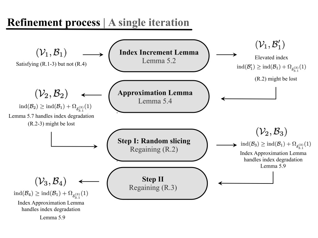
Figure 1: A single iteration of the refinement process

If the pair $\Pi^{\prime}$ satisfies Property (R.4), then the proof concludes; otherwise another iteration of the refinement process takes place, this time with $\Pi^{\prime}$ assuming the role of $\Pi$ above. The index increment argument and the fact that the index of any pair of partitions is bounded from above by one (see 5.3), imply that such a refinement process must terminate. Therefore, within $O(1)$ iterations, a pair of partitions satisfying Properties (R.1-4) is encountered and Lemma 3.1 is proved. Figure 1 provides a bird’s eye view of a single iteration of the refinement process.

Initial partitions. The first pair of partitions, namely $\mathcal{V}_{0}$ and $\mathcal{B}_{0}$, from which the proof of Lemma 3.1 commences is defined next. Let $V$ denote the common vertex-set of $H_{1},\ldots,H_{s_{\ref{lem:ghrl}}}$ and let $\mathcal{V}_{0}$ be an equitable vertex-partition of the form $V=V_{1}\mathbin{\mathchoice{\leavevmode\vtop{\halign{\hfil$\m@th\displaystyle#$\hfil\cr\cup\cr\cdot\crcr}}}{\leavevmode\vtop{\halign{\hfil$\m@th\textstyle#$\hfil\cr\cup\cr\cdot\crcr}}}{\leavevmode\vtop{\halign{\hfil$\m@th\scriptstyle#$\hfil\cr\cup\cr\cdot\crcr}}}{\leavevmode\vtop{\halign{\hfil$\m@th\scriptscriptstyle#$\hfil\cr\cup\cr\cdot\crcr}}}}\cdots\mathbin{\mathchoice{\leavevmode\vtop{\halign{\hfil$\m@th\displaystyle#$\hfil\cr\cup\cr\cdot\crcr}}}{\leavevmode\vtop{\halign{\hfil$\m@th\textstyle#$\hfil\cr\cup\cr\cdot\crcr}}}{\leavevmode\vtop{\halign{\hfil$\m@th\scriptstyle#$\hfil\cr\cup\cr\cdot\crcr}}}{\leavevmode\vtop{\halign{\hfil$\m@th\scriptscriptstyle#$\hfil\cr\cup\cr\cdot\crcr}}}}V_{t}$, with $t$ some positive integer, such that $H_{i}$ is $\delta^{(2)}_{\ref{lem:ghrl}}(\ell_{\ref{lem:ghrl}})$-weakly-regular with respect to $\mathcal{V}_{0}$ for every $i\in[s_{\ref{lem:ghrl}}]$. Such a partition exists by the Weak Lemma (Lemma 2.5) applied with

$$t_{\ref{lem:weak}}\gg\max\left\{(\delta^{(3)}_{\ref{lem:ghrl}})^{-4},t_{\ref{lem:ghrl}}\right\},$$ (5.1)

$\delta_{\ref{lem:weak}}=\delta^{(2)}_{\ref{lem:ghrl}}(\ell_{\ref{lem:ghrl}})$, the trivial partition $\mathcal{U}_{\ref{lem:weak}}=V$ (i.e., $h_{\ref{lem:weak}}=1$), and the given sequence $H_{1},\ldots,H_{s_{\ref{lem:ghrl}}}$. In preparation for a subsequent application of Lemma 5.2 (stated below), one may further assume that $t$ is sufficiently large so as to ensure that $e(K^{(3)}(\mathcal{V}_{0}))\geq(1-\delta^{(3)}_{\ref{lem:ghrl}}/2)\binom{|V|}{3}$ holds (and thus have 5.4, stated below, satisfied).

Let $\mathcal{B}_{0}$ be the partition of $K^{(2)}(\mathcal{V}_{0})$ defined as follows. For every $1\leq i<j\leq t$, let $B^{ij}_{1},\ldots,B^{ij}_{\ell_{\ref{lem:ghrl}}}$ be a uniform random edge-colouring of $K^{(2)}(V_{i},V_{j})$ using $\ell_{\ref{lem:ghrl}}$ colours. That is, every edge of $K^{(2)}(V_{i},V_{j})$ is assigned a colour from $[\ell_{\ref{lem:ghrl}}]$ uniformly at random and independently of all other edges of $K^{(2)}(V_{i},V_{j})$. For every $k\in[\ell_{\ref{lem:ghrl}}]$, every pair of indices $1\leq i<j\leq t$, and any pair of subsets $X\subseteq V_{i}$ and $Y\subseteq V_{j}$, it holds that

$$\operatorname{\mathbb{E}}\left[e\left(B^{ij}_{k}[X,Y]\right)\right]=\frac{1}{\ell_{\ref{lem:ghrl}}}|X||Y|.$$

Applying Chernoff’s inequality [34, Theorem 2.1] yields

$$\mathbb{P}\left[\Big{|}e\left(B^{ij}_{k}[X,Y]\right)-\frac{1}{\ell_{\ref{lem:ghrl}}}|X||Y|\Big{|}>\delta^{(2)}_{\ref{lem:ghrl}}(\ell_{\ref{lem:ghrl}})|V_{i}||V_{j}|\right]=\exp(-\Omega(n^{2})),$$

where here we rely on $\mathcal{V}$ being equitable, implying that $|V_{i}|,|V_{j}|=\Omega(n)$. A union-bound over all choices of $k,i,j,X$, and $Y$ implies that a.a.s. $B^{ij}_{k}$ is $(\delta^{(2)}_{\ref{lem:ghrl}}(\ell_{\ref{lem:ghrl}}),\ell_{\ref{lem:ghrl}}^{-1})$-regular for every $k\in[\ell_{\ref{lem:ghrl}}]$ and every pair of indices $1\leq i<j\leq t$. In particular, $\mathcal{B}_{0}$ is $\ell_{\ref{lem:ghrl}}$-equitable.

Index increment. The notion of index, employed in our arguments, is defined next, along with the index increment machinery alluded to above. Let $V$ be a finite set and let $\mathcal{V}$ be the partition given by $V=V_{1}\mathbin{\mathchoice{\leavevmode\vtop{\halign{\hfil$\m@th\displaystyle#$\hfil\cr\cup\cr\cdot\crcr}}}{\leavevmode\vtop{\halign{\hfil$\m@th\textstyle#$\hfil\cr\cup\cr\cdot\crcr}}}{\leavevmode\vtop{\halign{\hfil$\m@th\scriptstyle#$\hfil\cr\cup\cr\cdot\crcr}}}{\leavevmode\vtop{\halign{\hfil$\m@th\scriptscriptstyle#$\hfil\cr\cup\cr\cdot\crcr}}}}\ldots\mathbin{\mathchoice{\leavevmode\vtop{\halign{\hfil$\m@th\displaystyle#$\hfil\cr\cup\cr\cdot\crcr}}}{\leavevmode\vtop{\halign{\hfil$\m@th\textstyle#$\hfil\cr\cup\cr\cdot\crcr}}}{\leavevmode\vtop{\halign{\hfil$\m@th\scriptstyle#$\hfil\cr\cup\cr\cdot\crcr}}}{\leavevmode\vtop{\halign{\hfil$\m@th\scriptscriptstyle#$\hfil\cr\cup\cr\cdot\crcr}}}}V_{h}$, with $h\geq 1$ some integer. Let $\mathcal{B}$ be an $\ell$-equitable partition with respect to $\mathcal{V}$, for some integer $\ell\geq 1$. The index of $\mathcal{B}$ with respect to $\mathcal{V}$ and a partition $\mathcal{H}$ of $[V]^{3}$ is given by

$$\mathrm{ind}(\mathcal{B})=\frac{1}{|V|^{3}}\sum_{H\in\mathcal{H}}\sum_{P}d\left(H|P\right)^{2}\cdot|\mathcal{K}_{3}(P)|,$$ (5.2)

where the second sum ranges over the triads of $\mathcal{B}$. It is known (see [57, Fact 33]) that

$$\mathrm{ind}(\mathcal{B})\in[0,1].$$ (5.3)

The notion of the index, seen in 5.2, fits the case $s_{\ref{lem:ghrl}}=1$, i.e., the case in which a single hypergraph $H$ is to be regularised. In this case, the members of the partition $\mathcal{H}$, seen in 5.2, are $H$ and its complement; this is in accordance with [57] (see the implication of [57, Theorem 17] from [57, Theorem 23]). Our formulation of Lemma 3.1 supports $s_{\ref{lem:ghrl}}>1$; in the terminology of [39], it is a multi-colour regularity lemma. To support the multi-colour version, the standard approach (see, e.g., [39]) is to define the above index for each hypergraph (and its complement) being regularised and then define a new notion of index given by the average of all of the aforementioned indices of the individual hypergaphs (taking the average ensures that the new index is upperbounded by one as well).

Remark 5.1.

As the transition to the multi-coloured version is considered standard, we prove Lemma 3.1 under the assumption that $s_{\ref{lem:ghrl}}=1$. Our proof of Theorem 1.4 does not employ the multi-colour version.

Lemma 5.2.

(Index Increment Lemma [57, Proposition 39]) Let $V$ be a finite set, let $\mathcal{V}$ be a partition of $V$, let $\mathcal{H}$ be a partition of $[V]^{3}$, and let $\mathcal{B}$ be an $\ell$-equitable partition of $K^{(2)}(\mathcal{V})$. Furthermore, let an integer $r:=r_{\ref{lem:index-inc}}\geq 1$ be given and let $\delta:=\delta_{\ref{lem:index-inc}}>0$ satisfy

$$e\left(K^{(3)}(\mathcal{V})\right)\geq(1-\delta/2)\binom{|V|}{3}.$$ (5.4)

If there exists an $H\in\mathcal{H}$ that is $(\delta,r)$-irregular with respect to $\mathcal{B}$, then there exists a partition $\mathcal{B}^{\prime}$ of $[V]^{2}$ satisfying

(INC.1)

$\mathcal{B}^{\prime}\prec\mathcal{B}$,

(INC.2)

$|\mathcal{B}^{\prime}|\leq|\mathcal{B}|\cdot 2^{r|\mathcal{V}|\ell^{2}}\leq|\mathcal{V}|^{2}\ell\cdot 2^{r|\mathcal{V}|\ell^{2}}$, and

(INC.3)

$\mathrm{ind}(\mathcal{B}^{\prime})\geq\mathrm{ind}(\mathcal{B})+\delta^{4}/2$.

Remark 5.3.

The partitions $\mathcal{B}$ and $\mathcal{B^{\prime}}$, appearing in the premise of Lemma 5.2, are taken over $K^{(2)}(\mathcal{V})$ and $[V]^{2}$, respectively. In Section 2.2, it is explained what is meant by stating that a partition of $[V]^{2}$ refines a partition of $K^{(2)}(\mathcal{V})$.

Returning to the general scheme of the proof outline, let $(\mathcal{V}_{1},\mathcal{B}_{1})$ be a pair of partitions from which a single iteration of the refinement process commences; these partitions satisfy Properties (R.1-3) but they do not satisfy Property (R.4). The Index Increment Lemma (Lemma 5.2) applied to $(\mathcal{V}_{1},\mathcal{B}_{1})$ produces a pair $(\mathcal{V}_{1},\mathcal{B}^{\prime}_{1})$ with $\mathcal{B}_{1}$ and $\mathcal{B}^{\prime}_{1}$ satisfying (INC.1-3). That is, $\mathcal{B}^{\prime}_{1}$ refines $\mathcal{B}_{1}$, its size is $O(|\mathcal{B}_{1}|)=O(1)$, and most importantly satisfies $\mathrm{ind}(\mathcal{B}^{\prime}_{1})\geq\mathrm{ind}(\mathcal{B})+\Omega_{\delta^{(3)}_{\ref{lem:ghrl}}}(1)$. While $\mathcal{B}^{\prime}_{1}$ has its index elevated appropriately relative to $\mathcal{B}_{1}$, it may have lost Property (R.2). Indeed, $\mathcal{B}^{\prime}_{1}$ arises from considering the Venn diagram of all witnesses of $(\delta^{(3)}_{\ref{lem:ghrl}},r_{\ref{lem:ghrl}})$-irregularity that the sequence $(H_{1},\ldots,H_{s_{\ref{lem:ghrl}}})$ has across $(\mathcal{V}_{1},\mathcal{B}_{1})$; see [57] for further details. The process then continues with further refinements of $(\mathcal{V}_{1},\mathcal{B}^{\prime}_{1})$ so as to regain Property (R.2).

Approximation. The next result of [57] serves as a key tool through which we regain Property (R.2). It is a generalisation of a result from [9] which handles the corresponding graph case.

Lemma 5.4.

(The Approximation Lemma [57, Lemma 25]) For every pair of integers $s:=s_{\ref{lem:approx}}\geq 1$ and $h:=h_{\ref{lem:approx}}\geq 1$, every real number $\nu:=\nu_{\ref{lem:approx}}>0$, and every function $\varepsilon:=\varepsilon_{\ref{lem:approx}}:\mathbb{N}\to(0,1]$, there exist positive integers $t_{\ref{lem:approx}}$ and $n_{0}$ such that the following holds whenever $n\geq n_{0}$. Let $V$ be a finite set of size $n$, let $\mathcal{V}$ be a partition of the form $V=V_{1}\mathbin{\mathchoice{\leavevmode\vtop{\halign{\hfil$\m@th\displaystyle#$\hfil\cr\cup\cr\cdot\crcr}}}{\leavevmode\vtop{\halign{\hfil$\m@th\textstyle#$\hfil\cr\cup\cr\cdot\crcr}}}{\leavevmode\vtop{\halign{\hfil$\m@th\scriptstyle#$\hfil\cr\cup\cr\cdot\crcr}}}{\leavevmode\vtop{\halign{\hfil$\m@th\scriptscriptstyle#$\hfil\cr\cup\cr\cdot\crcr}}}}\cdots\mathbin{\mathchoice{\leavevmode\vtop{\halign{\hfil$\m@th\displaystyle#$\hfil\cr\cup\cr\cdot\crcr}}}{\leavevmode\vtop{\halign{\hfil$\m@th\textstyle#$\hfil\cr\cup\cr\cdot\crcr}}}{\leavevmode\vtop{\halign{\hfil$\m@th\scriptstyle#$\hfil\cr\cup\cr\cdot\crcr}}}{\leavevmode\vtop{\halign{\hfil$\m@th\scriptscriptstyle#$\hfil\cr\cup\cr\cdot\crcr}}}}V_{h}$ with all its parts having size $\Omega(n)$, and let $\mathcal{B}:=(B_{1},\ldots,B_{s})$ be a partition of $[V]^{2}$. Then, there exists an equitable partition $\{V=U_{1}\mathbin{\mathchoice{\leavevmode\vtop{\halign{\hfil$\m@th\displaystyle#$\hfil\cr\cup\cr\cdot\crcr}}}{\leavevmode\vtop{\halign{\hfil$\m@th\textstyle#$\hfil\cr\cup\cr\cdot\crcr}}}{\leavevmode\vtop{\halign{\hfil$\m@th\scriptstyle#$\hfil\cr\cup\cr\cdot\crcr}}}{\leavevmode\vtop{\halign{\hfil$\m@th\scriptscriptstyle#$\hfil\cr\cup\cr\cdot\crcr}}}}\cdots\mathbin{\mathchoice{\leavevmode\vtop{\halign{\hfil$\m@th\displaystyle#$\hfil\cr\cup\cr\cdot\crcr}}}{\leavevmode\vtop{\halign{\hfil$\m@th\textstyle#$\hfil\cr\cup\cr\cdot\crcr}}}{\leavevmode\vtop{\halign{\hfil$\m@th\scriptstyle#$\hfil\cr\cup\cr\cdot\crcr}}}{\leavevmode\vtop{\halign{\hfil$\m@th\scriptscriptstyle#$\hfil\cr\cup\cr\cdot\crcr}}}}U_{t_{\ref{lem:approx}}}\}\prec\mathcal{V}$, namely $\mathcal{U}$, as well as a partition $\mathcal{B}^{\prime}:=(B^{\prime}_{1},\ldots,B^{\prime}_{s})$ of $[V]^{2}$ such that the following holds.

(APX.1)

$B^{\prime}_{k}[U_{i},U_{j}]$ is $\varepsilon(t_{\ref{lem:approx}})$-regular for every $k\in[s]$ and every $1\leq i<j\leq t_{\ref{lem:approx}}$.

(APX.2)

$|E(B_{i})\triangle E(B^{\prime}_{i})|\leq\nu n^{2}$ for every $i\in[s]$.

Remark 5.5.

The Approximation Lemma bares its name as it replaces every $B\in\mathcal{B}$ with a highly regular bipartite graph $B^{\prime}$ of virtually the same density as $B$ (as specified in (APX.2)). However, $B^{\prime}$ need not be a subgraph of $B$ and may contain edges not present in $B$; the latter degrades the index increment attained by the Index Increment Lemma (Lemma 5.2).

Remark 5.6.

In its original formulation, namely [57, Lemma 25], the approximation lemma also entails a divisibility condition which in our formulation would read as $t_{\ref{lem:approx}}!\mid n$. The term $t_{\ref{lem:approx}}!$ is a fixed constant. In the case that $t_{\ref{lem:approx}}!\nmid n$ holds, our formulation takes into account any degradation of all parameters that may be incurred by having to distribute at most $t_{\ref{lem:approx}}!$ vertices amongst the members of $\mathcal{U}$.

Returning to the pair $(\mathcal{V}_{1},\mathcal{B}^{\prime}_{1})$ and its potential loss of Property (R.2), the Approximation Lemma (Lemma 5.4) is applied to this pair so as to produce a pair $(\mathcal{V}_{2},\mathcal{B}_{2})$ such that $\mathcal{V}_{2}\prec\mathcal{V}_{1}$ and $\mathcal{B}_{2}$ approximates $\mathcal{B}^{\prime}_{1}$ per (APX.2). That is, modulo some $\xi n^{2}$ exceptional pairs, with $\xi>0$ being arbitrarily small yet fixed, the partition $\mathcal{B}_{2}$ refines $\mathcal{B}^{\prime}_{1}$. Utilising the fact that the members of $\mathcal{B}_{2}$ are highly regular, per (APX.1), we proceed to randomly slice (see Steps I.a and  I.b in the proof of Lemma 3.1 for details) the members of $\mathcal{B}_{2}$ so as to obtain a partition $\mathcal{B}_{3}$ which, modulo some $\xi^{\prime}n^{2}$ exceptions, with $\xi^{\prime}>0$ being arbitrarily small yet fixed, refines $\mathcal{B}_{2}$ and such that its members satisfy Property (R.2), in that all its members are at the ‘correct’ density and regularity as required by Property (R.2). This stage of the process culminates with the pair $(\mathcal{V}_{2},\mathcal{B}_{3})$ and with Property (R.2) regained. Having $\mathcal{B}_{2}$ essentially refining $\mathcal{B}^{\prime}_{1}$ and $\mathcal{B}_{3}$ essentially refining $\mathcal{B}_{2}$ modulo some $o(n^{2})$ exceptions each time, plays a crucial part in the forthcoming index manipulation arguments appearing below. Unfortunately, due to the application of the Approximation Lemma (Lemma 5.4), it is possible that the pair $(\mathcal{V}_{2},\mathcal{B}_{3})$ does not satisfy Property (R.3).

Weak regularity re-established. To regain Property (R.3), the Weak Lemma (Lemma 2.5) is applied to $\mathcal{V}_{2}$ so as to attain a vertex-partition, namely $\mathcal{V}_{3}$, such that $\mathcal{V}_{3}\prec\mathcal{V}_{2}$ and such that $H$ is weakly-regular with respect to $\mathcal{V}_{3}$ at the required level. This in turn affects the regularity of the members of $\mathcal{B}_{3}$ with respect to the members of $\mathcal{V}_{3}$ in the sense that the satisfaction of Property (R.2) is again in jeopardy. Repeated applications of the Slicing Lemma (Lemma 2.3) are then used to regain Property (R.2) once more. The key point at this stage is that the degradation in the regularity of the members of $\mathcal{B}_{3}$, with respect to $\mathcal{V}_{3}$, can be anticipated prior to the application of the Approximation Lemma (Lemma 5.4) which in turn allows for an application of the latter with an enhanced regularity threshold, in order to compensate for this eventual degradation.

This stage ends with a pair $(\mathcal{V}_{3},\mathcal{B}_{4})$, where $\mathcal{B}_{4}\prec\mathcal{B}_{3}$ and is the result of the aforementioned repeated applications of the Slicing Lemma (Lemma 2.3). Accurate details regarding this stage can be seen in Step II of the proof of Lemma 3.1.

Index manipulations. Tracking the index of the various partitions encountered throughout the process described above, we start with the inequality $\mathrm{ind}(\mathcal{B}^{\prime}_{1})\geq\mathrm{ind}(\mathcal{B}_{1})+\Omega_{\delta^{(3)}_{\ref{lem:ghrl}}}(1)$ supported by the Index Increment Lemma (Lemma 5.2). From here on out this index increment suffers degradation incurred by the refinement process outlined above. Two tools are used to curb this degradation. The first such tool, stated below in Lemma 5.7, is designed to handle the index of partitions produced by the Approximation Lemma (Lemma 5.4). The second is the Index Approximation Lemma (see Lemma 5.9 below) which provides estimates for the index of all partitions encountered with the exception of the one produced by the Approximation Lemma (Lemma 5.4).

Lemma 5.7.

[57, Proposition 34] Let $s:=s_{\ref{lem:index-approx}},h:=h_{\ref{lem:index-approx}}$, and $t:=t_{\ref{lem:index-approx}}\geq h$ be positive integers and let $\nu:=\nu_{\ref{lem:index-approx}}>0$. Let $V$ be a set of size $n$ and let $\mathcal{V}=V_{1}\mathbin{\mathchoice{\leavevmode\vtop{\halign{\hfil$\m@th\displaystyle#$\hfil\cr\cup\cr\cdot\crcr}}}{\leavevmode\vtop{\halign{\hfil$\m@th\textstyle#$\hfil\cr\cup\cr\cdot\crcr}}}{\leavevmode\vtop{\halign{\hfil$\m@th\scriptstyle#$\hfil\cr\cup\cr\cdot\crcr}}}{\leavevmode\vtop{\halign{\hfil$\m@th\scriptscriptstyle#$\hfil\cr\cup\cr\cdot\crcr}}}}\cdots\mathbin{\mathchoice{\leavevmode\vtop{\halign{\hfil$\m@th\displaystyle#$\hfil\cr\cup\cr\cdot\crcr}}}{\leavevmode\vtop{\halign{\hfil$\m@th\textstyle#$\hfil\cr\cup\cr\cdot\crcr}}}{\leavevmode\vtop{\halign{\hfil$\m@th\scriptstyle#$\hfil\cr\cup\cr\cdot\crcr}}}{\leavevmode\vtop{\halign{\hfil$\m@th\scriptscriptstyle#$\hfil\cr\cup\cr\cdot\crcr}}}}V_{h}$ and $\mathcal{U}=U_{1}\mathbin{\mathchoice{\leavevmode\vtop{\halign{\hfil$\m@th\displaystyle#$\hfil\cr\cup\cr\cdot\crcr}}}{\leavevmode\vtop{\halign{\hfil$\m@th\textstyle#$\hfil\cr\cup\cr\cdot\crcr}}}{\leavevmode\vtop{\halign{\hfil$\m@th\scriptstyle#$\hfil\cr\cup\cr\cdot\crcr}}}{\leavevmode\vtop{\halign{\hfil$\m@th\scriptscriptstyle#$\hfil\cr\cup\cr\cdot\crcr}}}}\cdots\mathbin{\mathchoice{\leavevmode\vtop{\halign{\hfil$\m@th\displaystyle#$\hfil\cr\cup\cr\cdot\crcr}}}{\leavevmode\vtop{\halign{\hfil$\m@th\textstyle#$\hfil\cr\cup\cr\cdot\crcr}}}{\leavevmode\vtop{\halign{\hfil$\m@th\scriptstyle#$\hfil\cr\cup\cr\cdot\crcr}}}{\leavevmode\vtop{\halign{\hfil$\m@th\scriptscriptstyle#$\hfil\cr\cup\cr\cdot\crcr}}}}U_{t}$ be partitions of $V$ such that $\mathcal{U}\prec\mathcal{V}$. Let $\mathcal{H}$ be a partition of $[V]^{3}$ and let $\mathcal{B}:=(B_{1},\ldots,B_{s})$ and $\mathcal{B}^{\prime}:=(B^{\prime}_{1},\ldots,B^{\prime}_{s})$ be partitions of $K^{(2)}(\mathcal{V})$ and $K^{(2)}(\mathcal{U})$, respectively, satisfying $|E(B_{i})\triangle E(B^{\prime}_{i})|\leq\nu n^{2}$ for every $i\in[s]$. Then,

$$\mathrm{ind}(\mathcal{B^{\prime}})\geq\mathrm{ind}(\mathcal{B})-9(2s)^{3}\nu$$ (5.5)

holds, where $\mathrm{ind}(\mathcal{B})$ is taken with respect to $\mathcal{V}$ and $\mathcal{H}$, and $\mathrm{ind}(\mathcal{B^{\prime}})$ is taken with respect to $\mathcal{U}$ and $\mathcal{H}$.

Remark 5.8.

The partitions $\mathcal{B}$ and $\mathcal{B}^{\prime}$ defined in Lemma 5.7 can both be viewed as partitions of $[V]^{2}$ (see Section 2.2) so as to fit the formulation of the Approximation Lemma (Lemma 5.4) and of [57, Proposition 34]. The latter, fits more general settings than the one appearing in its adaptation stated in Lemma 5.7.

The partition $\mathcal{B}_{2}$ is produced by the Approximation Lemma (Lemma 5.4) applied to $(\mathcal{V}_{1},\mathcal{B}^{\prime}_{1})$. Lemma 5.7 coupled with a judicious choice of $\nu_{\ref{lem:approx}}$ made upon applying the Approximation Lemma (and prior to the application of the Index Approximation Lemma), yields

$$\mathrm{ind}(\mathcal{B}_{2})\geq\mathrm{ind}(\mathcal{B}^{\prime}_{1})-\nu^{\prime}_{\ref{lem:approx}}\geq\mathrm{ind}(\mathcal{B}_{1})+\Omega_{\delta^{(3)}_{\ref{lem:ghrl}}}(1)-\nu^{\prime}_{\ref{lem:approx}},$$

where $\nu^{\prime}_{\ref{lem:approx}}>0$ is a constant related to $\nu_{\ref{lem:approx}}$ through 5.5. Being able to anticipate this degradation of the index allows for an appropriate choice of $\nu_{\ref{lem:approx}}$ to be passed to the Approximation Lemma so as to render $\mathrm{ind}(\mathcal{B}_{2})\geq\mathrm{ind}(\mathcal{B}_{1})+\Omega_{\delta^{(3)}_{\ref{lem:ghrl}}}(1)$.

The second tool for curbing the degradation of the index, namely the Index Approximation Lemma, is stated next. Let $\mathcal{V}$ be a partition of a finite set $V$ and let $\mathcal{B}$ and $\mathcal{B}^{\prime}$ be partitions of $K^{(2)}(\mathcal{V})$. Given a non-negative real number $\beta$, a partition $\mathcal{B}^{\prime}$ is said to form a $\beta$-refinement of a partition $\mathcal{B}$, denoted $\mathcal{B^{\prime}}\prec_{\beta}\mathcal{B}$, if $\sum e(B^{\prime})\leq\beta|V|^{2}$, where the sum is extended over $\{B^{\prime}\in\mathcal{B}^{\prime}:B^{\prime}\not\subseteq B\;\text{for every}\;B\in\mathcal{B}\}$. The following lemma asserts that a partition of $K^{(2)}(\mathcal{V})$ that $\beta$-refines another partition of $K^{(2)}(\mathcal{V})$ has its index at most $\beta$ ‘away’ from that of the partition being refined.

Lemma 5.9.

(The Index Approximation Lemma [57, Proposition 38]) Let $\beta$ be a non-negative real number, let $\mathcal{V}$ be a partition of a finite set $V$, let $\mathcal{B}$ and $\mathcal{B}^{\prime}$ be partitions of $K^{(2)}(\mathcal{V})$, and let $\mathcal{H}$ be a partition of $[V]^{3}$. If $\mathcal{B}^{\prime}\prec_{\beta}\mathcal{B}$, then $\mathrm{ind}(\mathcal{B}^{\prime})\geq\mathrm{ind}(\mathcal{B})-\beta$, where here the index is taken with respect to $\mathcal{V}$ and $\mathcal{H}$.

The next degradation in the index is incurred through the production of the partition $\mathcal{B}_{3}$ from $\mathcal{B}_{2}$ via random slicing. We prove that $\mathcal{B}_{3}$ forms a $\beta$-refinement of $\mathcal{B}_{2}$, where $\beta>0$ is small enough to ensure that $\mathrm{ind}(\mathcal{B}_{3})\geq\mathrm{ind}(\mathcal{B}_{1})+\Omega_{\delta^{(3)}_{\ref{lem:ghrl}}}(1)$ can still be inferred. The last partition, namely $\mathcal{B}_{4}$, properly refines $\mathcal{B}_{3}$, i.e. $\mathcal{B}_{4}\prec_{0}\mathcal{B}_{3}$, and thus, by the Index Approximation Lemma, no index degradation is incurred in the production of $\mathcal{B}_{4}$ culminating with $\mathrm{ind}(\mathcal{B}_{4})\geq\mathrm{ind}(\mathcal{B}_{1})+\Omega_{\delta^{(3)}_{\ref{lem:ghrl}}}(1)$.

Remark 5.10.

Upon the termination of the entire refinement process, a pair of partitions $(\mathcal{V},\mathcal{B})$ satisfying Properties (R.1-4) is produced. Setting $t=|\mathcal{V}|$ and $T_{\ref{lem:ghrl}}=|\mathcal{B}|$, yields $t\leq T_{\ref{lem:ghrl}}$ as well as $\ell\leq T_{\ref{lem:ghrl}}$, where $\ell$ and $t$ are per the premise of Lemma 3.1.

5.2 Proof of Lemma 3.1

Let $\delta_{3}:=\delta^{(3)}_{\ref{lem:ghrl}},\delta_{2}:=\delta^{(2)}_{\ref{lem:ghrl}},r:=r_{\ref{lem:ghrl}},\ell_{\ref{lem:ghrl}},t_{\ref{lem:ghrl}},s_{\ref{lem:ghrl}}$ and $(H_{1},\ldots,H_{s_{\ref{lem:ghrl}}})$ be as specified in the premise of Lemma 3.1; recall Remark 5.1 where it is stipulated that we assume that $s_{\ref{lem:ghrl}}=1$ so that $H:=H_{1}=\cdots=H_{s_{\ref{lem:ghrl}}}$. It suffices to prove an index increment along a single iteration of the refinement process described in Section 5.1. To that end, let $V$ be the vertex-set of $H$ and let $\mathcal{V}_{1}$ be an equitable partition of the form $V=V_{1}\mathbin{\mathchoice{\leavevmode\vtop{\halign{\hfil$\m@th\displaystyle#$\hfil\cr\cup\cr\cdot\crcr}}}{\leavevmode\vtop{\halign{\hfil$\m@th\textstyle#$\hfil\cr\cup\cr\cdot\crcr}}}{\leavevmode\vtop{\halign{\hfil$\m@th\scriptstyle#$\hfil\cr\cup\cr\cdot\crcr}}}{\leavevmode\vtop{\halign{\hfil$\m@th\scriptscriptstyle#$\hfil\cr\cup\cr\cdot\crcr}}}}\cdots\mathbin{\mathchoice{\leavevmode\vtop{\halign{\hfil$\m@th\displaystyle#$\hfil\cr\cup\cr\cdot\crcr}}}{\leavevmode\vtop{\halign{\hfil$\m@th\textstyle#$\hfil\cr\cup\cr\cdot\crcr}}}{\leavevmode\vtop{\halign{\hfil$\m@th\scriptstyle#$\hfil\cr\cup\cr\cdot\crcr}}}{\leavevmode\vtop{\halign{\hfil$\m@th\scriptscriptstyle#$\hfil\cr\cup\cr\cdot\crcr}}}}V_{t_{1}}$, with $t_{1}$ some positive integer, such that $H$ is $\delta_{2}(\ell_{1})$-weakly-regular with respect to $\mathcal{V}_{1}$, where $\ell_{1}$ is some positive integer. Let $\mathcal{B}_{1}$ be an $\ell_{1}$-equitable partition of $K^{(2)}(\mathcal{V}_{1})$. Assume that $e(K^{(3)}(\mathcal{V}_{1}))\geq(1-\delta_{3}/2)\binom{|V|}{3}$ holds and that the partitions $\mathcal{V}_{1}$ and $\mathcal{B}_{1}$ satisfy Properties (R.1-3) yet fail to satisfy Property (R.4). The Index Increment Lemma (Lemma 5.2) applied with $\delta_{\ref{lem:index-inc}}=\delta_{3}$ and $r_{\ref{lem:index-inc}}=r(t_{1},\ell_{1})$, asserts that there exists a partition $\mathcal{B}^{\prime}_{1}$ of $K^{(2)}(\mathcal{V}_{1})$ refining $\mathcal{B}_{1}$ such that $\ell_{2}:=|\mathcal{B}^{\prime}_{1}|\leq t^{2}_{1}\ell_{1}\cdot 2^{r(t_{1},\ell_{1})t_{1}\ell_{1}^{2}}$ and $\mathrm{ind}(\mathcal{B}^{\prime}_{1})\geq\mathrm{ind}(\mathcal{B}_{1})+\delta^{4}_{3}/2$. For future reference, we record that

$$\ell_{2}\gg\delta_{3}^{-4}$$ (5.6)

holds; this on account of $\ell_{2}\geq t_{1}\overset{\hyperref@@ii[eq:initial-t]{\textup{\tagform@{\ref*{eq:initial-t}}}}}{\gg}\delta_{3}^{-4}$.

We proceed with a two stage argument, captured below in Step I and Step II, through which the pair $(\mathcal{V}_{1},\mathcal{B}^{\prime}_{1})$ is further refined so as to obtain a pair of partitions satisfying Properties (R.1-3) and whose index is appropriately elevated with respect to that of $\mathcal{B}_{1}$.

Step I - Regaining Property (R.2). Let $\mathcal{V}_{2}$ and $\mathcal{B}_{2}$ be the vertex and pair partitions, respectively, whose existence is guaranteed by the Approximation Lemma (Lemma 5.4) applied to $\mathcal{V}_{1}$ and $\mathcal{B}^{\prime}_{1}$ with

$$s_{\ref{lem:approx}}=|\mathcal{B}^{\prime}_{1}|=\ell_{2},\quad h_{\ref{lem:approx}}=t_{1},\quad\nu:=\nu_{\ref{lem:approx}}\ll\frac{\delta^{4}_{3}}{s^{3}_{\ref{lem:approx}}},\quad\varepsilon_{\ref{lem:approx}}:=\varepsilon/C_{1}$$ (5.7)

where $C_{1}\gg\ell_{2}^{2}$ is some auxiliary constant and for every $\tilde{t}\in\mathbb{N}$

$$\varepsilon(\tilde{t}):=\min\left\{\ell_{2}^{-2},\frac{\delta_{2}(\ell_{2}^{2})}{T^{2}_{\ref{lem:weak}}(\tilde{t},\delta_{2}(\ell_{2}^{2}))}\right\}.$$ (5.8)

The partition $\mathcal{V}_{2}$ refines $\mathcal{V}_{1}$ and has the form $V=U_{1}\mathbin{\mathchoice{\leavevmode\vtop{\halign{\hfil$\m@th\displaystyle#$\hfil\cr\cup\cr\cdot\crcr}}}{\leavevmode\vtop{\halign{\hfil$\m@th\textstyle#$\hfil\cr\cup\cr\cdot\crcr}}}{\leavevmode\vtop{\halign{\hfil$\m@th\scriptstyle#$\hfil\cr\cup\cr\cdot\crcr}}}{\leavevmode\vtop{\halign{\hfil$\m@th\scriptscriptstyle#$\hfil\cr\cup\cr\cdot\crcr}}}}U_{2}\cdots\mathbin{\mathchoice{\leavevmode\vtop{\halign{\hfil$\m@th\displaystyle#$\hfil\cr\cup\cr\cdot\crcr}}}{\leavevmode\vtop{\halign{\hfil$\m@th\textstyle#$\hfil\cr\cup\cr\cdot\crcr}}}{\leavevmode\vtop{\halign{\hfil$\m@th\scriptstyle#$\hfil\cr\cup\cr\cdot\crcr}}}{\leavevmode\vtop{\halign{\hfil$\m@th\scriptscriptstyle#$\hfil\cr\cup\cr\cdot\crcr}}}}U_{t_{2}}$, where $t_{2}=t_{\ref{lem:approx}}(h_{\ref{lem:approx}},s_{\ref{lem:approx}},\nu,\varepsilon_{\ref{lem:approx}})$ and the last four parameters are as seen in 5.7. Each member $B\in\mathcal{B}_{2}$ has the property that $B[U_{i},U_{j}]$ is $\varepsilon_{\ref{lem:approx}}(t_{2})$-regular whenever $i,j\in[t_{2}]$ are distinct. In addition, the members of $\mathcal{B}_{2}$ approximate the densities of the members of $\mathcal{B}^{\prime}_{1}$ per (APX.2).

Fix indices $1\leq i<j\leq t_{2}$. In what follows, the members of $\mathcal{B}_{2}^{ij}:=\left\{B[U_{i},U_{j}]:B\in\mathcal{B}_{2}\right\}$ are sliced so as to yield a collection of $\ell_{2}^{2}$ bipartite graphs such that each of them is $(\varepsilon(t_{2}),\ell_{2}^{-2})$-regular. This is attained through randomly slicing each member of $\mathcal{B}_{2}^{ij}$ so that, with positive probability, each slice thus produced across all choices for $i$ and $j$ has the specified density and regularity. All this is carried out in two steps, namely Steps I.a and I.b. In the first step, the so-called dense members of $\mathcal{B}^{ij}$ are sliced; in the second step the so-called sparse members of $\mathcal{B}^{ij}$ are sliced along with leftovers incurred through the slicing of the dense members.

Step I.a: Random slicing of dense parts. Fix indices $1\leq i<j\leq t_{2}$ and let $\mathcal{D}^{ij}:=\left\{B[U_{i},U_{j}]:B\in\mathcal{B}_{2}\;\text{and}\;d(B[U_{i},U_{j}])\geq\ell_{2}^{-2}\right\}$ denote the members of $\mathcal{B}_{2}^{ij}$ that are sufficiently dense; note that $\mathcal{D}^{ij}\neq\emptyset$ since the members of $\mathcal{B}_{2}^{ij}$ partition $K^{(2)}(U_{i},U_{j})$ and $|\mathcal{B}_{2}^{ij}|=\ell_{2}$. For every $\Gamma\in\mathcal{D}^{ij}$, there exist an integer $0\leq k_{\Gamma}\leq\ell_{2}^{2}$ and a real number $0\leq\eta_{\Gamma}<\ell_{2}^{-2}$ such that $d(\Gamma)=\frac{k_{\Gamma}}{\ell_{2}^{2}}+\eta_{\Gamma}$. Colour the members of $E(\Gamma)$ by assigning each edge a colour from the palette $\{0,\ldots,k_{\Gamma}\}$, independently from the rest of the edges, according to the following scheme:

1. An edge of $\Gamma$ is assigned the colour $0$ with probability $\frac{\eta_{\Gamma}}{d(\Gamma)}$.

2. An edge of $\Gamma$ is assigned the colour $1\leq i\leq k_{\Gamma}$ with probability $\frac{1}{\ell_{2}^{2}d(\Gamma)}$.

Note that

$$\frac{k_{\Gamma}}{\ell_{2}^{2}d(\Gamma)}+\frac{\eta_{\Gamma}}{d(\Gamma)}=\frac{1}{d(\Gamma)}\left(\frac{k_{\Gamma}}{\ell_{2}^{2}}+\eta_{\Gamma}\right)=1.$$

Let $\Gamma_{0},\Gamma_{1},\ldots,\Gamma_{k_{\Gamma}}$ denote the random pairwise edge-disjoint subgraphs of $\Gamma$ resulting from such a colouring. The random subgraph $\Gamma_{0}$ is referred to as the trash subgraph.

Set $C_{2}=C_{1}/2$ and note that an appropriate choice of $C_{1}$ ensures that $C_{2}\gg\ell_{2}^{2}$ holds. Fix a constant $\zeta$ satisfying

$$0<\zeta\ll\min\left\{\ell_{2}^{-2},\varepsilon(t_{2})/C_{1}\right\}$$ (5.9)

and

$$\left\lfloor\frac{1}{\ell_{2}^{-2}-\zeta}\right\rfloor=\ell_{2}^{2}=\left\lceil\frac{1}{\ell_{2}^{-2}+\zeta}\right\rceil\quad\text{and}\quad\zeta+\max_{\Gamma\in\mathcal{D}^{ij}}\eta_{\Gamma}<\ell_{2}^{-2}.$$ (5.10)

Consider the events

$$\mathcal{E}_{0}(\Gamma) :=\left\{d(\Gamma_{0})\leq\eta_{\Gamma}+\zeta\right\},$$

$$\mathcal{E}_{1}(\Gamma) :=\left\{d(\Gamma_{i})=\ell_{2}^{-2}\pm\zeta\;\text{for every}\;1\leq i\leq k_{\Gamma}\right\},$$

$$\mathcal{E}_{2}(\Gamma) :=\left\{\text{$\Gamma_{i}$ is $(\varepsilon(t_{2})/C_{2},\ell_{2}^{-2})$-regular for every $1\leq i\leq k_{\Gamma}$}\right\}.$$

Finally, for every $k\in\{0,1,2\}$, let

$$\mathcal{E}_{k}:=\{\text{$\mathcal{E}_{k}(\Gamma)$ holds for all $\Gamma\in\mathcal{D}^{ij}$ and for all indices $1\leq i<j\leq t_{2}$}\}.$$

We claim that

$$\mathbb{P}[\mathcal{E}_{0}\wedge\mathcal{E}_{1}\wedge\mathcal{E}_{2}]>0.$$ (5.11)

Note that the number of pairs of indices $1\leq i<j\leq t_{2}$ is independent of $n$. Moreover, $|\mathcal{D}^{ij}|$ is independent of $n$ for any given pair of indices $1\leq i<j\leq t_{2}$.

Hence, in order to prove 5.11, it suffices to prove that

$$\mathbb{P}[\mathcal{E}_{0}(\Gamma)\wedge\mathcal{E}_{1}(\Gamma)\wedge\mathcal{E}_{2}(\Gamma)]=1-o_{n}(1)$$ (5.12)

for every pair of indices $1\leq i<j\leq t_{2}$ and every $\Gamma\in\mathcal{D}^{ij}$.

Note that $\mathcal{E}_{1}$ is not part of the formulation of Property (R.2) but rather an auxiliary event facilitating our arguments seen in Step I.b below. On the other hand, $\mathcal{E}_{2}$ is directly related to Property (R.2) and is of prime concern in regaining Property (R.2).

As noted above, to conclude Step I.a, it remains to prove 5.12. We begin by noting that $\operatorname{\mathbb{E}}[e(\Gamma_{0})]=\eta_{\Gamma}|U_{i}||U_{j}|$ and that $\operatorname{\mathbb{E}}[e(\Gamma_{h})]=\frac{1}{\ell_{2}^{2}}|U_{i}||U_{j}|$ holds for every $1\leq h\leq k_{\Gamma}$. Then, owing to Chernoff’s inequality [34, Theorem 2.1 and Corollary 2.3], we may write

$$\mathbb{P} \left[e(\Gamma_{0})\geq(\eta_{\Gamma}+\zeta)|U_{i}||U_{j}|\right]\leq\exp\left(-\frac{(\zeta|U_{i}||U_{j}|)^{2}}{2(\eta_{\Gamma}+\zeta)|U_{i}||U_{j}|}\right)=\exp\left(-\Omega(n^{2})\right),$$

$$\mathbb{P} \left[\left|e(\Gamma_{h})-\ell_{2}^{-2}|U_{i}||U_{j}|\right|\geq\zeta|U_{i}||U_{j}|\right]\leq\exp(-\Omega(|U_{i}||U_{j}|))=\exp\left(-\Omega(n^{2})\right),$$

where the last equalities seen for each of the bounds just specified, are owing to $\mathcal{V}_{2}$ being equitable, leading to $|U_{i}|=\Omega(n)$ holding for every $i\in[t_{2}]$. In particular, each of the events $\mathcal{E}_{0}(\Gamma)$ and $\mathcal{E}_{1}(\Gamma)$ holds asymptotically almost surely.

To estimate the probability that $\mathcal{E}_{2}(\Gamma)$ holds, fix $X\subseteq U_{i}$ and $Y\subseteq U_{j}$, and recall that

$$e(\Gamma[X,Y])=d(\Gamma)|X||Y|\pm\varepsilon_{\ref{lem:approx}}(t_{2})|U_{i}||U_{j}|.$$

For every $1\leq h\leq k_{\Gamma}$, it holds that

$$\operatorname{\mathbb{E}}[e(\Gamma_{h}[X,Y])] =\ell_{2}^{-2}|X||Y|\pm\frac{\varepsilon_{\ref{lem:approx}}(t_{2})}{\ell_{2}^{2}d(\Gamma)}|U_{i}||U_{j}|$$

$$=\ell_{2}^{-2}|X||Y|\pm\frac{\varepsilon(t_{2})}{C_{1}\ell_{2}^{2}d(\Gamma)}|U_{i}||U_{j}|$$

$$=\ell_{2}^{-2}|X||Y|\pm\frac{\varepsilon(t_{2})}{C_{1}}|U_{i}||U_{j}|,$$

where the last equality holds since $\Gamma\in\mathcal{D}^{ij}$ and thus $\ell_{2}^{2}d(\Gamma)\geq 1$. It then follows by Chernoff’s inequality [34, Theorem 2.1] that

$$\mathbb{P}\left[e(\Gamma_{h}[X,Y])\geq\ell_{2}^{-2}|X||Y|+\frac{\varepsilon(t_{2})}{C_{1}}|U_{i}||U_{j}|+\zeta|U_{i}||U_{j}|\right] =\exp(-\Omega(n^{2}))$$

and

$$\mathbb{P}\left[e(\Gamma_{h}[X,Y])\leq\ell_{2}^{-2}|X||Y|-\frac{\varepsilon(t_{2})}{C_{1}}|U_{i}||U_{j}|-\zeta|U_{i}||U_{j}|\right] =\exp(-\Omega(n^{2}))$$

both hold. The number of choices for the sets $X$ and $Y$ is at most $2^{2n}$ and the number of choices for $h$ is $k_{\Gamma}$. Since, moreover, $C_{2}=C_{1}/2\gg\ell_{2}^{2}$ and $\zeta$ satisfies 5.9, it follows that the random subgraph $\Gamma_{h}$ is a.a.s. $(\varepsilon(t_{2})/C_{2},\ell_{2}^{-2})$-regular for every $1\leq h\leq k_{\Gamma}$. This shows that $\mathcal{E}_{2}(\Gamma)$ holds a.a.s. and thus concludes the proof of 5.12.

Step I.b: Randomly slicing the trash and sparse members of $\boldsymbol{\mathcal{B}_{2}^{ij}}$. Fix indices $1\leq i<j\leq t_{2}$. Expose $\Gamma_{0},\Gamma_{1},\ldots,\Gamma_{k_{\Gamma}}$ for every $\Gamma\in\mathcal{D}^{ij}$. Let $M=\bigcup_{\Gamma\in\mathcal{D}^{ij}}\bigcup_{i=1}^{k_{\Gamma}}\Gamma_{i}$ and let $L=K^{(2)}(U_{i},U_{j})\setminus M$. Let $k=\sum_{\Gamma\in\mathcal{D}^{ij}}k_{\Gamma}$ so that one may write $M=\bigcup_{i=1}^{k}S_{i}$, where $S_{i}$ is $(\varepsilon(t_{2})/C_{2},\ell_{2}^{-2})$-regular with density $d(S_{i})=\ell_{2}^{-2}\pm\zeta$ for every $i\in[k]$. Note that $k\leq\ell_{2}^{2}$ holds by the first equality appearing in 5.10.

Since $S_{1},\ldots,S_{k}$ are pairwise edge-disjoint, $M$ is $\left(\frac{k\varepsilon(t_{2})}{C_{2}},\frac{k}{\ell_{2}^{2}}\right)$-regular. The (bipartite) complement of $M$ in $K^{(2)}(U_{i},U_{j})$, namely $L$, is then $\left(\frac{k\varepsilon(t_{2})}{C_{2}},\frac{\ell_{2}^{2}-k}{\ell_{2}^{2}}\right)$-regular, by Observation 2.4. Slice $L$ uniformly at random using $c:=\ell_{2}^{2}-k$ colours; let $L_{1},\ldots,L_{c}$ denote the resulting slices (note that $c>0$ as $L$ contains $\Gamma_{0}$ for every $\Gamma\in\mathcal{D}^{ij}$ and is thus dense). To gauge the regularity of $L_{h}$, where $h\in[c]$, note that for a fixed $X\subseteq U_{i}$ and $Y\subseteq U_{j}$, one has

$$\operatorname{\mathbb{E}}[e_{L_{h}}(X,Y)]=\ell_{2}^{-2}|X||Y|\pm\frac{k\varepsilon(t_{2})}{C_{2}\cdot c}|U_{i}||U_{j}|=\ell_{2}^{-2}|X||Y|\pm\frac{\varepsilon(t_{2})}{C_{3}}|U_{i}||U_{j}|$$

where $C_{3}=C_{2}\cdot c/k$; an appropriate choice of $C_{1}$ ensures that $C_{3}\gg\ell_{2}^{2}$ holds. An application of Chernoff’s inequality (with deviation $\zeta^{\prime}|U_{i}||U_{j}|$, where $0<\zeta^{\prime}\ll\varepsilon(t_{2})/C_{3}$), yields that a.a.s. $L_{h}$ is $(\varepsilon(t_{2})/C_{4},\ell_{2}^{-2})$-regular, where $C_{4}\gg\ell_{2}^{2}$ is some constant. Since $c$ is independent of $n$, it follows that a.a.s. all of the aforementioned slices admit this level of regularity.

We conclude Step I by setting $\mathcal{B}_{3}$ to denote the collection of all slices produced in Steps I.a and I.b. As such, $\mathcal{B}_{3}$ partitions $K^{(2)}(\mathcal{V}_{2})$ but need not be a refinement of $\mathcal{B}_{2}$ on account of Step I.b. In addition, $\mathcal{B}_{3}$ is $\ell_{2}^{2}$-equitable (indeed, for every pair of indices $1\leq i<j\in t_{2}$, some $k\leq\ell_{2}^{2}$ slices are created in Steps I.a and $\ell_{2}^{2}-k$ additional slices are created in I.b) with each of its members being $(\varepsilon(t_{2}),\ell_{2}^{-2})$-regular. The pair of partitions $(\mathcal{V}_{2},\mathcal{B}_{3})$ then satisfies Property (R.2) with the aforementioned parameters.

Step II: Regaining Property (R.3). In this step, we produce an equitable vertex partition $\mathcal{V}_{3}$ such that $\mathcal{V}_{3}\prec\mathcal{V}_{2}$ and subsequently a partition $\mathcal{B}_{4}$ of $K^{(2)}(\mathcal{V}_{3})$ such that the pair $(\mathcal{V}_{3},\mathcal{B}_{4})$ satisfies Properties (R.1-3) with the correct parameters.

Let $\mathcal{V}_{3}$ be the equitable vertex partition resulting from an application of the Weak Lemma (Lemma 2.5) with $\mathcal{V}_{2}$ as the initial vertex partition and along with

$$\delta_{\ref{lem:weak}}=\delta_{2}\left(\ell_{2}^{2}\right)\quad\text{and}\quad t_{\ref{lem:weak}}=t_{2}.$$

Recall that $\mathcal{V}_{2}$ has the form $V=U_{1}\mathbin{\mathchoice{\leavevmode\vtop{\halign{\hfil$\m@th\displaystyle#$\hfil\cr\cup\cr\cdot\crcr}}}{\leavevmode\vtop{\halign{\hfil$\m@th\textstyle#$\hfil\cr\cup\cr\cdot\crcr}}}{\leavevmode\vtop{\halign{\hfil$\m@th\scriptstyle#$\hfil\cr\cup\cr\cdot\crcr}}}{\leavevmode\vtop{\halign{\hfil$\m@th\scriptscriptstyle#$\hfil\cr\cup\cr\cdot\crcr}}}}\cdots\mathbin{\mathchoice{\leavevmode\vtop{\halign{\hfil$\m@th\displaystyle#$\hfil\cr\cup\cr\cdot\crcr}}}{\leavevmode\vtop{\halign{\hfil$\m@th\textstyle#$\hfil\cr\cup\cr\cdot\crcr}}}{\leavevmode\vtop{\halign{\hfil$\m@th\scriptstyle#$\hfil\cr\cup\cr\cdot\crcr}}}{\leavevmode\vtop{\halign{\hfil$\m@th\scriptscriptstyle#$\hfil\cr\cup\cr\cdot\crcr}}}}U_{t_{2}}$ and that $\mathcal{V}_{3}\prec\mathcal{V}_{2}$. Since both $\mathcal{V}_{2}$ and $\mathcal{V}_{3}$ are equitable, it follows that the number of members of $\mathcal{V}_{3}$ refining a single cluster of $\mathcal{V}_{2}$ is uniform across all clusters of $\mathcal{V}_{2}$. For a pair of distinct indices $i,j\in[t_{2}]$, let

$$\mathcal{W}^{(i)}=\left\{W^{(i)}_{1},\ldots,W^{(i)}_{z}\right\}\quad\text{and}\quad\mathcal{W}^{(j)}=\left\{W^{(j)}_{1},\ldots,W^{(j)}_{z}\right\}$$

denote the members of $\mathcal{V}_{3}$ refining $U_{i}$ and $U_{j}$, respectively. In addition, let $\mathcal{B}_{3}^{ij}$ consist of the members of $\mathcal{B}_{3}$ partitioning $K^{(2)}(U_{i},U_{j})$; recall that $|\mathcal{B}_{3}^{ij}|=\ell_{2}^{2}$.

Fix some $W\in\mathcal{W}^{(i)}$, $W^{\prime}\in\mathcal{W}^{(j)}$, and $\Gamma\in\mathcal{B}^{ij}_{3}$. We claim that $\Gamma[W,W^{\prime}]$ is $(\delta_{2}(\ell_{2}^{2}),\ell_{2}^{-2})$-regular. Indeed, note first that $|W|,|W^{\prime}|\geq\frac{n}{T_{\ref{lem:weak}}(t_{2},\delta_{2}\left(\ell_{2}^{2}\right))}$ and that $T_{\ref{lem:weak}}(t_{2},\delta_{2}\left(\ell_{2}^{2}\right))^{-1}\geq\varepsilon(t_{2})$, where the latter inequality holds by 5.8. Hence, an application of the Slicing Lemma (Lemma 2.3) with

$$d_{\ref{lem:slicing}}=\ell_{2}^{-2},\quad\delta_{\ref{lem:slicing}}=\varepsilon(t_{2}),\quad\alpha_{\ref{lem:slicing}}=T_{\ref{lem:weak}}(t_{2},\delta_{2}\left(\ell_{2}^{2}\right))^{-1}$$

implies that $\Gamma[W,W^{\prime}]$ is $\left(\xi,\ell_{2}^{-2}\pm\delta_{\ref{lem:slicing}}\right)$-regular, with

$$\xi=\max\left\{T_{\ref{lem:weak}}(t_{2},\delta_{2}\left(\ell_{2}^{2}\right))\delta_{\ref{lem:slicing}},2\delta_{\ref{lem:slicing}}\right\}\leq\frac{\delta_{2}(\ell_{2}^{2})}{T_{\ref{lem:weak}}(t_{2},\delta_{2}\left(\ell_{2}^{2}\right))},$$

where the above inequality holds by 5.8. We may then absorb the deviation in the density by enlarging the error term to deduce that $\Gamma[W,W^{\prime}]$ is $(\delta_{2}(\ell_{2}^{2}),\ell_{2}^{-2})$-regular, as claimed.

We conclude that the members of $\mathcal{B}_{3}^{ij}$ define $\ell_{2}^{2}$ edge-disjoint $(\delta_{2}(\ell_{2}^{2}),\ell_{2}^{-2})$-regular subgraphs, between every pair of sets $W\in\mathcal{W}^{(i)}$ and $W^{\prime}\in\mathcal{W}^{(j)}$. Moreover, these subgraphs partition $K^{(2)}(W,W^{\prime})$. Define $\mathcal{B}_{4}$ to be the partition of $K^{(2)}(\mathcal{V}_{3})$ whose members are the subgraphs of the form $\Gamma[W,W^{\prime}]$, where $W\in\mathcal{W}^{(i)}$, $W^{\prime}\in\mathcal{W}^{(j)}$, and $1\leq i<j\leq t_{2}$; note that $\mathcal{B}_{4}\prec\mathcal{B}_{3}$.

Index increment. We conclude the proof of Lemma 3.1 by tracking the index of the various partitions defined throughout the refinement process above and prove that this process culminates with the last partition, namely $\mathcal{B}_{4}$, satisfying

$$\mathrm{ind}(\mathcal{B}_{4})\geq\mathrm{ind}(\mathcal{B}_{1})+\delta_{3}^{4}/8.$$ (5.13)

The refinement process commences with the Index Increment Lemma (Lemma 5.2) yielding $\mathrm{ind}(\mathcal{B}^{\prime}_{1})\geq\mathrm{ind}(\mathcal{B}_{1})+\delta_{3}^{4}/2$, where here the index is taken with respect to $\mathcal{V}_{1}$ and the partition $\mathcal{H}$ whose members are $H$ and its complement. The pair of partitions $(\mathcal{V}_{2},\mathcal{B}_{2})$ is obtained through an application of the Approximation Lemma (Lemma 5.4) to the pair $(\mathcal{V}_{1},\mathcal{B}^{\prime}_{1})$. It follows that

$$\mathrm{ind}(\mathcal{B}_{2})\overset{\hyperref@@ii[eq:ind-approx-new]{\textup{\tagform@{\ref*{eq:ind-approx-new}}}}}{\geq}\mathrm{ind}(\mathcal{B}^{\prime}_{1})-9(2s)^{3}\nu\overset{\hyperref@@ii[eq:const]{\textup{\tagform@{\ref*{eq:const}}}}}{\geq}\mathrm{ind}(\mathcal{B}_{1})+\delta_{3}^{4}/4$$

holds.

The partition $\mathcal{B}_{3}$ need not be a refinement of $\mathcal{B}_{2}$; this is due to the treatment of sparse and trash subgraphs of $\mathcal{B}_{2}$ seen in Step I.b, where these subgraphs are united and then collectively sliced. The partition $\mathcal{B}_{2}$ is obtained from partition $\mathcal{B}^{\prime}_{1}$ through the Approximation Lemma (Lemma 5.4) and thus $|\mathcal{B}_{2}|=|\mathcal{B}^{\prime}_{1}|=\ell_{2}$ holds. Let $\mathcal{A}_{3}=\{B_{3}\in\mathcal{B}_{3}:B_{3}\not\subseteq B_{2}\text{ for every }B_{2}\in\mathcal{B}_{2}\}$. Then,

$$\sum_{A\in\mathcal{A}_{3}}e(A) \overset{\phantom{\hyperref@@ii[eq:zeta2]{\textup{\tagform@{\ref*{eq:zeta2}}}}}}{\leq}\sum_{1\leq i<j\leq t_{2}}\left(\sum_{\Gamma\in\mathcal{D}^{ij}}e(\Gamma_{0})+\sum_{\Gamma\in\mathcal{B}_{2}^{ij}\setminus\mathcal{D}^{ij}}e(\Gamma)\right)$$

$$\overset{\phantom{\hyperref@@ii[eq:zeta2]{\textup{\tagform@{\ref*{eq:zeta2}}}}}}{\leq}|\mathcal{B}_{2}|\left(\zeta+\max_{\Gamma\in\mathcal{D}^{ij}}\eta_{\Gamma}\right)n^{2}+|\mathcal{B}_{2}|\cdot\ell_{2}^{-2}n^{2}$$

$$\overset{\hyperref@@ii[eq:zeta2]{\textup{\tagform@{\ref*{eq:zeta2}}}}}{\leq}2\ell_{2}^{-1}n^{2}.$$

It follows that $\mathcal{B}_{3}$ is a $(2\ell_{2}^{-1})$-refinement of $\mathcal{B}_{2}$ and thus

$$\mathrm{ind}(\mathcal{B}_{3})\geq\mathrm{ind}(\mathcal{B}_{1})+\delta_{3}^{4}/4-2\ell_{2}^{-1}\overset{\hyperref@@ii[eq:ell_2]{\textup{\tagform@{\ref*{eq:ell_2}}}}}{\geq}\mathrm{ind}(\mathcal{B}_{1})+\delta_{3}^{4}/8$$

holds, by the Index Approximation Lemma (Lemma 5.9).

The last partition, namely $\mathcal{B}_{4}$, is attained from $\mathcal{B}_{3}$ through repeated applications of the Slicing Lemma (Lemma 2.3). As such $\mathcal{B}_{4}\prec_{0}\mathcal{B}_{3}$ and thus $\mathrm{ind}(\mathcal{B}_{4})\geq\mathrm{ind}(\mathcal{B}_{3})$ holds by the Index Approximation Lemma (Lemma 5.9). This proves 5.13 as required.

Conclusion. The fact that the index of a partition is bounded from above by one (see 5.3) coupled with the index increment obtained in each iteration of the refinement process, lead to a pair of partitions satisfying Properties (R.1-4) being encountered within $O(\delta_{3}^{-4})$ iterations of this process. This concludes the proof of the Strong Graph-Like hypergraph regularity lemma for $3$-graphs (Lemma 3.1).

6 Proof of the Tuple Lemma

Given $t,\varepsilon,$ and $d_{3}$ per the premise of Lemma 3.5, set an auxiliary constant

$$0<\zeta\ll\min\left\{\varepsilon,d_{3}^{t-1},1\right\}$$ (6.1)

and choose

$$0<\delta_{3}\ll\min\left\{(d_{3}^{t-1}-11\zeta)\zeta^{2},\zeta^{3}\right\}.$$ (6.2)

Given $0<d_{2}\ll d_{3}$, set

$$0<\delta_{2}\ll\min\left\{\frac{\zeta^{2}d_{2}^{6t}}{\max\{t,1\}},\zeta^{2}(d_{3}^{t-1}-\zeta)^{2}d_{2}^{8t+2}\right\}\quad\text{and}\quad r=\frac{\zeta}{d_{2}^{2t-2}}.$$ (6.3)

The assumption that $d_{2}\ll d_{3}$ appearing in the premise supports a choice of $\zeta$ which ensures that $r$ is a positive integer.

The proof is by induction on $t$. For $t=0$, the set defined through the intersection seen on the left hand side of 3.2 coincides with $E_{P}(Y,Z)$; indeed, in this case, no members of $X$ are taken into the tuple and thus no restriction is imposed through the aforementioned intersection. In this case,

$$e_{P}(Y,Z)=d_{2}|Y||Z|\pm\varepsilon d_{2}|Y||Z|$$

is asserted by 3.2 and this is supported by the assumption that $P$ forms a $(\delta_{2},d_{2})$-triad and $\delta_{2}\leq\varepsilon d_{2}$, holding by 6.3 and 6.1. Assume then that $t\geq 1$ and proceed to the induction step. Throughout this section, we employ the following notation for joint vertex-neighbourhoods and joint link graphs.

Definition 6.1.

Let $k$ be a positive integer. Given $\boldsymbol{x}\in X^{k}$, let

$$N_{P}(\boldsymbol{x},Y):=\left(\bigcap_{x\in\boldsymbol{x}}N_{P}(x)\right)\cap Y\quad\text{and}\quad N_{P}(\boldsymbol{x},Z):=\left(\bigcap_{x\in\boldsymbol{x}}N_{P}(x)\right)\cap Z$$

denote the joint vertex-neighbourhoods of the members of $\boldsymbol{x}$ in $Y$ and in $Z$, respectively. In addition, let

$$L_{H}(\boldsymbol{x},P):=\bigcap_{x\in\boldsymbol{x}}L_{H}(x,P)$$

denote the joint link graph of all members of $\boldsymbol{x}$ supported on $P$.

The core property pursued throughout the proof of Lemma 3.5 reads as follows.

Definition 6.2.

(Upper and lower extension properties for tuples) Let $t$ be a positive integer. A $(t-1)$-tuple $\boldsymbol{x}\in X^{t-1}$ is said to have the lower-$\gamma$-extension property if it satisfies the following properties simultaneously.

(E.1)

$$\left|N_{P}(\boldsymbol{x},Y)\right|=(1\pm\gamma)d_{2}^{t-1}|Y|\quad\text{and}\quad\left|N_{P}(\boldsymbol{x},Z)\right|=(1\pm\gamma)d_{2}^{t-1}|Z|;$$

(E.2)

$$e(L_{H}(\boldsymbol{x},P))=\left(d_{3}^{t-1}\pm\gamma\right)d_{2}^{2t-1}|Y||Z|;\;\text{and}$$

(E.3)

all but at most $\gamma|X|$ vertices $x\in X$ satisfy

$$e(L_{H}(\boldsymbol{x^{\prime}},P))\geq(d_{3}^{t}-13\gamma)d_{2}^{2t+1}|Y||Z|,$$ (6.4)

where $\boldsymbol{x^{\prime}}:=(\boldsymbol{x},x)$ is a $t$-tuple.

We say that $\boldsymbol{x}$ satisfies the upper-$\gamma$-extension property if $\boldsymbol{x}$ satisfies Properties (E.1-2) simultaneously along with

(E.4)

all but at most $\gamma|X|$ vertices $x\in X$ satisfy

$$e(L_{H}(\boldsymbol{x^{\prime}},P))\leq(d_{3}^{t}+13\gamma)d_{2}^{2t+1}|Y||Z|,$$ (6.5)

where $\boldsymbol{x^{\prime}}:=(\boldsymbol{x},x)$ is a $t$-tuple.

To establish the induction step, it suffices to prove that there exists a constant $\gamma\in(0,\varepsilon/13)$ such that

(L)

all but at most $\frac{\varepsilon}{2}|X|^{t-1}$ of the members of $X^{t-1}$ satisfy the lower-$\gamma$-extension property; and

(U)

all but at most $\frac{\varepsilon}{2}|X|^{t-1}$ of the members of $X^{t-1}$ satisfy the upper-$\gamma$-extension property.

Indeed, if there exists such a $\gamma$, then all but at most $\varepsilon|X|^{t-1}\cdot|X|+|X|^{t-1}\cdot\gamma|X|\leq 2\varepsilon|X|^{t}$ members of $X^{t}$ satisfy both the upper and lower bounds seen in 3.2 concluding the proof of the tuple lemma. In the sequel, we show that one may take $\gamma=\zeta$.

Let

$$\mathcal{T}:=\left\{\boldsymbol{x}\in X^{t-1}:\;\text{$\boldsymbol{x}$ satisfies Properties~{}(E.1-2) with $\gamma=\zeta$}\right\}.$$

We claim that

$$|\mathcal{T}|\geq\left(1-\frac{\zeta}{2}\right)|X|^{t-1}.$$ (6.6)

In order to prove 6.6, we consider properties (E.1) and (E.2) separately. Starting with Property (E.1), note that $P$ is a $(\delta_{2},d_{2})$-regular triad, where $(d_{2}\pm\delta_{2})^{t-1}=(1\pm\zeta)d_{2}^{t-1}$, owing to $\delta_{2}\ll\zeta d_{2}^{t}$ which holds by 6.3. Since, moreover, $\delta_{2}\ll\zeta/t$ holds by 6.3, it follows by Lemma 3.4 that all but at most $2\delta_{2}(t-1)|X|^{t-1}\leq\frac{\zeta}{4}|X|^{t-1}$ of the members of $X^{t-1}$ satisfy Property (E.1) with $\gamma=\zeta$. Next, it follows by the induction hypothesis, applied with $t_{\ref{lem:tuple}}=t-1$, $\varepsilon_{\ref{lem:tuple}}=\zeta/8$, and $d_{\ref{lem:tuple}}^{(3)}=d_{3}$, that all but at most $\frac{\zeta}{4}|X|^{t-1}$ of the members of $X^{t-1}$ satisfy Property (E.2) with $\gamma=\zeta$.

Having established 6.6, it suffices to prove the following two claims.

Claim 6.3.

All but at most $\frac{\varepsilon}{4}|X|^{t-1}$ of the members of $\mathcal{T}$ satisfy Property (E.3) with $\gamma=\zeta$.

Claim 6.4.

All but at most $\frac{\varepsilon}{4}|X|^{t-1}$ of the members of $\mathcal{T}$ satisfy Property (E.4) with $\gamma=\zeta$.

Indeed, if Claims 6.3 and 6.4 both hold, then coupled with 6.6, all but at most $\left(\frac{\varepsilon}{4}+\frac{\varepsilon}{4}+\frac{\zeta}{2}\right)|X|^{t-1}\overset{\hyperref@@ii[eq:zeta]{\textup{\tagform@{\ref*{eq:zeta}}}}}{\leq}\varepsilon|X|^{t-1}$ of the members of $X^{t-1}$ satisfy both the upper and lower $\zeta$-extension properties as required.

Define

$$\mathcal{B}_{L} :=\{\boldsymbol{x}\in\mathcal{T}:\boldsymbol{x}\;\text{fails to satisfy Property~{}(E.3) with $\gamma=\zeta$}\};$$

$$\mathcal{B}_{U} :=\{\boldsymbol{x}\in\mathcal{T}:\boldsymbol{x}\;\text{fails to satisfy Property~{}(E.4) with $\gamma=\zeta$}\}.$$

The next two claims assert that if $\mathcal{B}_{L}$ or $\mathcal{B}_{U}$ exceed a certain size, then $r$ pairwise disjoint $(t-1)$-tuples can be found in these sets, having the property that their joint neighbourhoods along $P$ in both $Y$ and $Z$ are ‘small’ (see 6.7 below). These tuples are then used in the proofs of Claims 6.3 and 6.4, respectively, in order to construct witnesses of irregularity contradicting the premise of Lemma 3.5.

Claim 6.5.

If $|\mathcal{B}_{L}|\geq\frac{\varepsilon}{4}|X|^{t-1}$, then there exists a collection of $r$ pairwise vertex-disjoint $(t-1)$-tuples, namely $\boldsymbol{x}_{1},\ldots,\boldsymbol{x}_{r}\in\mathcal{B}_{L}$, such that

$$\left|N_{P}(\boldsymbol{x}_{i},Y)\cap N_{P}(\boldsymbol{x}_{j},Y)\right|\leq 2d_{2}^{2(t-1)}|Y|\quad\text{and}\quad\left|N_{P}(\boldsymbol{x}_{i},Z)\cap N_{P}(\boldsymbol{x}_{j},Z)\right|\leq 2d_{2}^{2(t-1)}|Z|$$ (6.7)

holds for every $1\leq i<j\leq r$.

Proof.   Define an auxiliary graph $\Gamma$, where $V(\Gamma)=\mathcal{B}_{L}$ and two $(t-1)$-tuples in $\mathcal{B}_{L}$ are adjacent provided that they are disjoint and satisfy 6.7. It suffices to prove that

$$e(\Gamma)\geq\left(1-d_{2}^{2(t-1)}\right)\binom{|\mathcal{B}_{L}|}{2};$$ (6.8)

indeed, if 6.8 holds, then $\Gamma$ contains a complete subgraph of order at least $d_{2}^{-2(t-1)}\overset{\hyperref@@ii[eq:delta2-r]{\textup{\tagform@{\ref*{eq:delta2-r}}}}}{\geq}r$, by Turán’s theorem [59].

It remains to prove 6.8. First, note that any given $(t-1)$-tuple shares a vertex with at most $O(|X|^{t-2})$ other $(t-1)$-tuples. Consequently, at most $O(|X|^{2t-3})=o\left(|X|^{2(t-1)}\right)=o\left(\binom{\mathcal{B}_{L}}{2}\right)$ members of $\binom{\mathcal{B}_{L}}{2}$ are disqualified from forming an edge in $\Gamma$ due to not being disjoint. Second, note that since $\delta_{2}\ll\varepsilon^{2}d_{2}^{2t}/t$ holds by 6.3 and 6.1, and since $P$ forms a $(\delta_{2},d_{2})$-regular triad, it follows by Lemma 3.4 that at most

$$2\delta_{2}\cdot 2(t-1)\cdot|X|^{2(t-1)}\ll\frac{\varepsilon^{2}\cdot d_{2}^{2(t-1)}}{2^{10}}|\mathcal{B}_{L}|^{2}\leq\frac{d_{2}^{2(t-1)}}{2}\binom{|\mathcal{B}_{L}|}{2}$$

of the $2(t-1)$-tuples $\boldsymbol{x}\in X^{2(t-1)}$ satisfy $|N_{P}(\boldsymbol{x},Y)|>2d_{2}^{2(t-1)}|Y|$ or $|N_{P}(\boldsymbol{x},Z)|>2d_{2}^{2(t-1)}|Z|$. Hence, at most $\frac{d_{2}^{2(t-1)}}{2}\binom{|\mathcal{B}_{L}|}{2}$ members of $\binom{\mathcal{B}_{L}}{2}$ are disjoint but fail to satisfy 6.7. These two observations complete the proof of 6.8. $\square$

Claim 6.6.

If $|\mathcal{B}_{U}|\geq\frac{\varepsilon}{4}|X|^{t-1}$, then there exists a collection of $r$ pairwise vertex-disjoint $(t-1)$-tuples in $\mathcal{B}_{U}$ such that any two of them satisfy 6.7.

Our proof of Claim 6.6 is essentially the same as that of Claim 6.5; the details are thus omitted.

We proceed to prove Claims 6.3 and 6.4. Since our proofs of both claims are quite similar, we provide a detailed proof of Claim 6.3, but for Claim 6.4 we only account for the main differences between the two arguments.

Proof of Claim 6.3.   Suppose for a contradiction that $|\mathcal{B}_{L}|\geq\frac{\varepsilon}{4}|X|^{t-1}$ and let $\boldsymbol{x}_{1},\ldots,\boldsymbol{x}_{r}$ be a collection of $r$ pairwise-disjoint members of $\mathcal{B}_{L}$ satisfying 6.7; the existence of such a collection is ensured by Claim 6.5. With each $\boldsymbol{x}\in\{\boldsymbol{x}_{1},\ldots,\boldsymbol{x}_{r}\}$ we associate a subgraph $Q_{\boldsymbol{x}}\subseteq P$. We then prove that while $\left|\bigcup_{j=1}^{r}\mathcal{K}_{3}(Q_{\boldsymbol{x}_{j}})\right|\geq\delta_{3}|\mathcal{K}_{3}(P)|$ holds, the collection $(Q_{\boldsymbol{x}_{1}},\ldots,Q_{\boldsymbol{x}_{r}})$ fails to satisfy 2.3 (with the appropriate constants) and thus forms a witness of irregularity for $H$ with respect to $P$, contradicting the premise of the Tuple Lemma.

For every $\boldsymbol{x}\in\{\boldsymbol{x}_{1},\ldots,\boldsymbol{x}_{r}\}$, there exists a set $X_{\boldsymbol{x}}\subseteq X$ satisfying $|X_{\boldsymbol{x}}|=\zeta|X|$ (a quantity which we assume is integral) having the property that each of its members fails to satisfy 6.4 with $\gamma=\zeta$ if added to $\boldsymbol{x}$ so as to form a $t$-tuple. Since $\delta_{2}\ll\zeta$ holds by 6.3, it follows that $|X_{\boldsymbol{x}}|\geq\delta_{2}|X|$. Since $\mathcal{B}_{L}\subseteq\mathcal{T}$, the tuple $\boldsymbol{x}$ satisfies Property (E.1) with $\gamma=\zeta$. Since, moreover, $\zeta\leq 1/2$ by 6.1, and $\delta_{2}\ll d_{2}^{t-1}$ by 6.3, it follows that

$$|N_{P}(\boldsymbol{x},Y)|\geq(1-\zeta)d_{2}^{t-1}|Y|\geq\delta_{2}|Y|\quad\text{and}\quad|N_{P}(\boldsymbol{x},Z)|\geq(1-\zeta)d_{2}^{t-1}|Z|\geq\delta_{2}|Z|$$

These lower bounds on the cardinalities of $X_{\boldsymbol{x}}$, $N_{P}(\boldsymbol{x},Y)$, and $N_{P}(\boldsymbol{x},Z)$ together with the Slicing Lemma (Lemma 2.3) collectively imply that $P[X_{\boldsymbol{x}},N_{P}(\boldsymbol{x},Y)]$ and $P[X_{\boldsymbol{x}},N_{P}(\boldsymbol{x},Z)]$ are both $(\sqrt{\delta_{2}},d_{2}\pm\delta_{2})$-regular; indeed

$$\max\left\{\frac{\delta_{2}}{\zeta},\;\frac{\delta_{2}}{(1-\zeta)d_{2}^{t-1}},\;2\delta_{2}\right\}\ll\sqrt{\delta_{2}}$$

follows, as $\delta_{2}\ll\zeta^{2}d_{2}^{2(t-1)}$ holds by 6.3, and as $\zeta\leq 1-\zeta$ due to $\zeta\ll 1/2$ holding by 6.1. The Two-Sided Triangle Counting Lemma (Lemma 2.2) implies that

$$|\mathcal{K}_{3}(Q_{\boldsymbol{x}})|=\left(1\pm\zeta\right)\zeta\left(d_{3}^{t-1}\pm\zeta\right)d_{2}^{2t+1}|X||Y|Z|,$$ (6.9)

where

$$Q_{\boldsymbol{x}}:=P[X_{\boldsymbol{x}},N_{P}(\boldsymbol{x},Y)]\mathbin{\mathchoice{\leavevmode\vtop{\halign{\hfil$\m@th\displaystyle#$\hfil\cr\cup\cr\cdot\crcr}}}{\leavevmode\vtop{\halign{\hfil$\m@th\textstyle#$\hfil\cr\cup\cr\cdot\crcr}}}{\leavevmode\vtop{\halign{\hfil$\m@th\scriptstyle#$\hfil\cr\cup\cr\cdot\crcr}}}{\leavevmode\vtop{\halign{\hfil$\m@th\scriptscriptstyle#$\hfil\cr\cup\cr\cdot\crcr}}}}P[X_{\boldsymbol{x}},N_{P}(\boldsymbol{x},Z)]\mathbin{\mathchoice{\leavevmode\vtop{\halign{\hfil$\m@th\displaystyle#$\hfil\cr\cup\cr\cdot\crcr}}}{\leavevmode\vtop{\halign{\hfil$\m@th\textstyle#$\hfil\cr\cup\cr\cdot\crcr}}}{\leavevmode\vtop{\halign{\hfil$\m@th\scriptstyle#$\hfil\cr\cup\cr\cdot\crcr}}}{\leavevmode\vtop{\halign{\hfil$\m@th\scriptscriptstyle#$\hfil\cr\cup\cr\cdot\crcr}}}}L_{H}({\boldsymbol{x}},P)\subseteq P.$$ (6.10)

To see why the upper bound stipulated in 6.9 holds, note that the Two-Sided Triangle Counting Lemma applied to $Q_{\boldsymbol{x}}$ yields

$$|\mathcal{K}_{3}(Q_{\boldsymbol{x}})| \leq(d_{2}+\delta_{2}+\sqrt{\delta_{2}})(d_{2}+\delta_{2})|X_{\boldsymbol{x}}|e(L_{H}(\boldsymbol{x},P))+2\sqrt{\delta_{2}}|X_{\boldsymbol{x}}||N_{P}(\boldsymbol{x},Y)||N_{P}(\boldsymbol{x},Z)|$$

$$\leq d_{2}^{2}|X_{\boldsymbol{x}}|e(L_{H}(\boldsymbol{x},P))+5\sqrt{\delta_{2}}d_{2}|X_{\boldsymbol{x}}|e(L_{H}(\boldsymbol{x},P))+2\sqrt{\delta_{2}}|X_{\boldsymbol{x}}||Y||Z|.$$

where the last inequality is supported by $\delta_{2}\ll d_{2}$ which holds due to 6.3.

Since $\mathcal{B}_{L}\subseteq\mathcal{T}$, the tuple $\boldsymbol{x}$ satisfies Property (E.2) with $\gamma=\zeta$, implying that

$$e(L_{H}(\boldsymbol{x},P))\leq\left(d_{3}^{t-1}+\zeta\right)d_{2}^{2t-1}|Y||Z|.$$

Therefore,

$$|\mathcal{K}_{3}(Q_{\boldsymbol{x}})| \leq d_{2}^{2}(d_{3}^{t-1}+\zeta)d_{2}^{2t-1}|X_{\boldsymbol{x}}||Y||Z|+7\sqrt{\delta_{2}}|X_{\boldsymbol{x}}||Y||Z|$$

$$\leq\left(1+\zeta\right)(d_{3}^{t-1}+\zeta)d_{2}^{2t+1}|X_{\boldsymbol{x}}||Y||Z|$$

$$=\left(1+\zeta\right)\zeta(d_{3}^{t-1}+\zeta)d_{2}^{2t+1}|X||Y||Z|,$$

where for the last inequality we rely on $\delta_{2}\ll\zeta^{2}(d_{3}^{t-1}+\zeta)^{2}d_{2}^{4t+2}$, which holds by 6.3.

A similar argument delivers the lower bound seen in 6.9. Indeed, the Two-Sided Triangle Counting Lemma applied to $Q_{\boldsymbol{x}}$ also provides

$$|\mathcal{K}_{3}(Q_{\boldsymbol{x}})| \geq(d_{2}-\delta_{2}-\sqrt{\delta_{2}})(d_{2}-\delta_{2})|X_{\boldsymbol{x}}|e(L_{H}(\boldsymbol{x},P))-2\sqrt{\delta_{2}}|X_{\boldsymbol{x}}||Y||Z|$$

$$\geq\left(d_{3}^{t-1}-\zeta\right)d_{2}^{2t+1}|X_{\boldsymbol{x}}||Y||Z|-7\sqrt{\delta_{2}}|X_{\boldsymbol{x}}||Y||Z|$$

$$\geq\left(1-\zeta\right)\zeta\left(d_{3}^{t-1}-\zeta\right)d_{2}^{2t+1}|X||Y||Z|,$$

where the penultimate inequality relies on

$$e(L_{H}(\boldsymbol{x},P))\geq\left(d_{3}^{t-1}-\zeta\right)d_{2}^{2t-1}|Y||Z|,$$

which holds owing to $\boldsymbol{x}$ satisfying Property (E.2) with $\gamma=\zeta$, and the last inequality is owing to $\delta_{2}\ll\zeta^{2}(d_{3}^{t-1}-\zeta)^{2}d_{2}^{4t+2}$ which holds by 6.3. This completes the proof of 6.9.

We proceed to prove that the collection $(Q_{\boldsymbol{x}_{1}},\ldots,Q_{\boldsymbol{x}_{r}})$ satisfies $\left|\bigcup_{j=1}^{r}\mathcal{K}_{3}(Q_{\boldsymbol{x}_{j}})\right|\geq\delta_{3}|\mathcal{K}_{3}(P)|$. Note that

$$\left|\bigcup_{j=1}^{r}\mathcal{K}_{3}(Q_{\boldsymbol{x}_{j}})\right| \overset{\phantom{\hyperref@@ii[eq:K3s-Qx]{\textup{\tagform@{\ref*{eq:K3s-Qx}}}}}}{\geq}\sum_{j=1}^{r}|\mathcal{K}_{3}(Q_{\boldsymbol{x}_{j}})|-\sum_{1\leq i<j\leq r}|\mathcal{K}_{3}(Q_{\boldsymbol{x}_{i}})\cap\mathcal{K}_{3}(Q_{\boldsymbol{x}_{j}})|$$

$$\overset{\hyperref@@ii[eq:K3s-Qx]{\textup{\tagform@{\ref*{eq:K3s-Qx}}}}}{\geq}r\left(1-\zeta\right)\zeta\left(d_{3}^{t-1}-\zeta\right)d_{2}^{2t+1}|X||Y||Z|-\sum_{1\leq i<j\leq r}\left|\mathcal{K}_{3}(Q_{\boldsymbol{x}_{i}})\cap\mathcal{K}_{3}(Q_{\boldsymbol{x}_{j}})\right|.$$ (6.11)

Given indices $1\leq i<j\leq r$, a triangle found in $\mathcal{K}_{3}(Q_{\boldsymbol{x}_{i}})\cap\mathcal{K}_{3}(Q_{\boldsymbol{x}_{j}})$ has its vertices residing in the sets $X_{\boldsymbol{x}_{i}}\cap X_{\boldsymbol{x}_{j}}$, $N_{P}(\boldsymbol{x}_{i},Y)\cap N_{P}(\boldsymbol{x}_{j},Y)$, and $N_{P}(\boldsymbol{x}_{i},Z)\cap N_{P}(\boldsymbol{x}_{j},Z)$. If any of these sets has size at most a $\sqrt{\delta_{2}}$-fraction of its respective host, namely $X,Y,Z$, respectively, then

$$\left|\mathcal{K}_{3}(Q_{\boldsymbol{x}_{i}})\cap\mathcal{K}_{3}(Q_{\boldsymbol{x}_{j}})\right|\leq\sqrt{\delta_{2}}|X||Y||Z|.$$ (6.12)

In the complementary case, the subgraphs $P[X_{\boldsymbol{x}_{i}}\cap X_{\boldsymbol{x}_{j}},N_{P}(\boldsymbol{x}_{i},Y)\cap N_{P}(\boldsymbol{x}_{j},Y)]$, $P[X_{\boldsymbol{x}_{i}}\cap X_{\boldsymbol{x}_{j}},N_{P}(\boldsymbol{x}_{i},Z)\cap N_{P}(\boldsymbol{x}_{j},Z)]$, and $P[N_{P}(\boldsymbol{x}_{i},Y)\cap N_{P}(\boldsymbol{x}_{j},Y),N_{P}(\boldsymbol{x}_{i},Z)\cap N_{P}(\boldsymbol{x}_{j},Z)]$ are all $(\sqrt{\delta_{2}},d_{2}\pm\delta_{2})$-regular, by the Slicing Lemma (Lemma 2.3). Hence,

$$\left|\mathcal{K}_{3}(Q_{\boldsymbol{x}_{i}})\cap\mathcal{K}_{3}(Q_{\boldsymbol{x}_{j}})\right| \leq\left((d_{2}+\delta_{2})^{3}+4\sqrt{\delta_{2}}\right)|X_{\boldsymbol{x}_{i}}\cap X_{\boldsymbol{x}_{j}}||N_{P}(\boldsymbol{x}_{i},Y)\cap N_{P}(\boldsymbol{x}_{j},Y)||N_{P}(\boldsymbol{x}_{i},Z)\cap N_{P}(\boldsymbol{x}_{j},Z)|$$

$$\leq\left(d_{2}^{3}+3\delta_{2}d_{2}+4\sqrt{\delta_{2}}\right)\cdot\zeta|X|\cdot 2d_{2}^{2(t-1)}|Y|\cdot 2d_{2}^{2(t-1)}|Z|$$

$$\leq 8\zeta d_{2}^{4t-1}|X||Y||Z|$$ (6.13)

holds, where the first inequality holds by 2.1, the second inequality is supported by 6.7 which is satisfied by $\boldsymbol{x}_{i}$ and $\boldsymbol{x}_{j}$, and for the third inequality, we rely on $\delta_{2}\ll d_{2}^{6}$ supported by 6.3. Then,

$$\sum_{1\leq i<j\leq r}\left|\mathcal{K}_{3}(Q_{\boldsymbol{x}_{i}})\cap\mathcal{K}_{3}(Q_{\boldsymbol{x}_{j}})\right| \overset{\hyperref@@ii[eq:cap-small]{\textup{\tagform@{\ref*{eq:cap-small}}}},\hyperref@@ii[eq:cap-main-term]{\textup{\tagform@{\ref*{eq:cap-main-term}}}}}{\leq}r^{2}\left(\sqrt{\delta_{2}}+8\zeta d_{2}^{4t-1}\right)|X||Y||Z|$$

$$\overset{\phantom{\hyperref@@ii[eq:cap-small]{\textup{\tagform@{\ref*{eq:cap-small}}}},\hyperref@@ii[eq:cap-main-term]{\textup{\tagform@{\ref*{eq:cap-main-term}}}}}}{\leq}9r^{2}\zeta d_{2}^{4t-1}|X||Y||Z|,$$ (6.14)

where the last inequality is owing to $\delta_{2}\ll\zeta^{2}d_{2}^{8t-2}$, supported by 6.3. Substituting this last estimate into 6.11, we arrive at

$$\left|\bigcup_{j=1}^{r}\mathcal{K}_{3}(Q_{\boldsymbol{x}_{j}})\right| \overset{\phantom{\hyperref@@ii[eq:delta2-r]{\textup{\tagform@{\ref*{eq:delta2-r}}}}}}{\geq}r\left(1-\zeta\right)\zeta\left(d_{3}^{t-1}-\zeta\right)d_{2}^{2t+1}|X||Y||Z|-9r^{2}\zeta d_{2}^{4t-1}|X||Y||Z|$$

$$\overset{\phantom{\hyperref@@ii[eq:delta2-r]{\textup{\tagform@{\ref*{eq:delta2-r}}}}}}{\geq}\left(r\zeta d_{3}^{t-1}d_{2}^{2t+1}-r\zeta^{2}d_{3}^{t-1}d_{2}^{2t+1}-r\zeta^{2}d_{2}^{2t+1}-9r^{2}\zeta d_{2}^{4t-1}\right)|X||Y||Z|$$

$$\overset{\hyperref@@ii[eq:delta2-r]{\textup{\tagform@{\ref*{eq:delta2-r}}}}}{=}\left(d_{3}^{t-1}-\zeta d_{3}^{t-1}-\zeta-9\zeta\right)\zeta^{2}d_{2}^{3}|X||Y||Z|$$

$$\overset{\phantom{\hyperref@@ii[eq:delta2-r]{\textup{\tagform@{\ref*{eq:delta2-r}}}}}}{\geq}(d_{3}^{t-1}-11\zeta)\zeta^{2}d_{2}^{3}|X||Y||Z|$$ (6.15)

$$\overset{\phantom{\hyperref@@ii[eq:delta2-r]{\textup{\tagform@{\ref*{eq:delta2-r}}}}}}{\geq}2\delta_{3}d_{2}^{3}|X||Y||Z|$$

$$\overset{\phantom{\hyperref@@ii[eq:delta2-r]{\textup{\tagform@{\ref*{eq:delta2-r}}}}}}{\geq}\delta_{3}|\mathcal{K}_{3}(P)|.$$ (6.16)

The first inequality above holds by 6.9 and 6. For the penultimate inequality, we rely on $\delta_{3}\ll(d_{3}^{t-1}-11\zeta)\zeta^{2}$, which holds by 6.2 (as well as 6.1 asserting that $\zeta\ll d_{3}^{t-1}$). For the last inequality, note that $\delta_{2}\ll d_{2}^{3}$, which is supported by 6.3, and 2.1 collectively yield

$$|\mathcal{K}_{3}(P)|\leq(d_{2}^{3}+4\delta_{2})|X||Y||Z|\leq 2d_{2}^{3}|X||Y||Z|.$$

Gearing up towards examining 2.3 and proving that it fails to hold for $(Q_{\boldsymbol{x}_{1}},\ldots,Q_{\boldsymbol{x}_{r}})$, note that, in particular,

$$d_{3}\left|\bigcup_{j=1}^{r}\mathcal{K}_{3}(Q_{\boldsymbol{x}_{j}})\right|\overset{\hyperref@@ii[eq:lower-bound-witness']{\textup{\tagform@{\ref*{eq:lower-bound-witness'}}}}}{\geq}(d_{3}^{t}-11d_{3}\zeta)\zeta^{2}d_{2}^{3}|X||Y||Z|\geq(d_{3}^{t}-11\zeta)\zeta^{2}d_{2}^{3}|X||Y||Z|$$ (6.17)

holds. On the other hand,

$$\left|\bigcup_{j=1}^{r}\left(E_{H}\cap\mathcal{K}_{3}(Q_{\boldsymbol{x}_{j}})\right)\right| \overset{\phantom{\hyperref@@ii[eq:delta2-r]{\textup{\tagform@{\ref*{eq:delta2-r}}}}}}{\leq}\sum_{j=1}^{r}\left|E_{H}\cap\mathcal{K}_{3}(Q_{\boldsymbol{x}_{j}})\right|$$

$$\overset{\phantom{\hyperref@@ii[eq:delta2-r]{\textup{\tagform@{\ref*{eq:delta2-r}}}}}}{<}r\zeta|X|\cdot(d_{3}^{t}-12\zeta)d_{2}^{2t+1}|Y||Z|$$

$$\overset{\hyperref@@ii[eq:delta2-r]{\textup{\tagform@{\ref*{eq:delta2-r}}}}}{=}(d_{3}^{t}-12\zeta)\zeta^{2}d_{2}^{3}|X||Y||Z|,$$ (6.18)

where the second inequality holds since, by definition, for every $j\in[r]$, every member of $X_{\boldsymbol{x}_{j}}$ fails to satisfy 6.4 with $\gamma=\zeta$ if added to $\boldsymbol{x}_{j}$ so as to form a $t$-tuple.

Therefore,

$$\left|\Big{|}\bigcup_{j=1}^{r}\left(E_{H}\cap\mathcal{K}_{3}(Q_{\boldsymbol{x}})\right)\Big{|}-d_{3}\Big{|}\bigcup_{j=1}^{r}\mathcal{K}_{3}(Q_{\boldsymbol{x}_{j}})\Big{|}\right| \overset{\hyperref@@ii[eq:lower-bound-witness]{\textup{\tagform@{\ref*{eq:lower-bound-witness}}}}\hyperref@@ii[eq:upper-bound-witness]{\textup{\tagform@{\ref*{eq:upper-bound-witness}}}}}{\geq}\left|d_{3}^{t}-12\zeta-d_{3}^{t}+11\zeta\right|\zeta^{2}d_{2}^{3}|X||Y||Z|$$

$$\overset{\phantom{\hyperref@@ii[eq:lower-bound-witness]{\textup{\tagform@{\ref*{eq:lower-bound-witness}}}}\hyperref@@ii[eq:upper-bound-witness]{\textup{\tagform@{\ref*{eq:upper-bound-witness}}}}}}{=}\zeta^{3}d_{2}^{3}|X||Y||Z|$$

$$\overset{\phantom{\hyperref@@ii[eq:lower-bound-witness]{\textup{\tagform@{\ref*{eq:lower-bound-witness}}}}\hyperref@@ii[eq:upper-bound-witness]{\textup{\tagform@{\ref*{eq:upper-bound-witness}}}}}}{\gg}2\delta_{3}d_{2}^{3}|X||Y||Z|$$

$$\overset{\phantom{\hyperref@@ii[eq:lower-bound-witness]{\textup{\tagform@{\ref*{eq:lower-bound-witness}}}}\hyperref@@ii[eq:upper-bound-witness]{\textup{\tagform@{\ref*{eq:upper-bound-witness}}}}}}{\geq}\delta_{3}|\mathcal{K}_{3}(P)|.$$ (6.19)

For the penultimate inequality, we rely on $\delta_{3}\ll\zeta^{3}$ which holds by 6.2, and for the last inequality we rely, once more, on $|\mathcal{K}_{3}(P)|\leq 2d_{2}^{3}|X||Y||Z|$ which holds by 2.1.

To conclude the proof of Claim 6.3 and thus the lower bound seen in 3.2, note that 6.16 and 6.19 contradict the assumption that $H$ is $(\delta_{3},d_{3},r)$-regular with respect to $P$. $\square$

We proceed to the proof of Claim 6.4 which supports the upper bound seen in 3.2. As mentioned above, our proof of Claim 6.4 is quite similar to that seen for Claim 6.3; hence, we do not give a detailed proof of Claim 6.4, but rather specify the main points where our arguments diverge from their counterparts appearing in the proof of Claim 6.3.

Proof of Claim 6.4.   Suppose for a contradiction that $|\mathcal{B}_{U}|\geq\frac{\varepsilon}{4}|X|^{t-1}$ and let $\boldsymbol{x}_{1},\ldots,\boldsymbol{x}_{r}$ be a collection of $r$ pairwise-disjoint members of $\mathcal{B}_{U}$ satisfying 6.7; the existence of such a collection is ensured by Claim 6.6. For every $\boldsymbol{x}\in\{\boldsymbol{x}_{1},\ldots,\boldsymbol{x}_{r}\}$ there exists a set $X_{\boldsymbol{x}}\subseteq X$ of size $|X_{\boldsymbol{x}}|=\zeta|X|$, having the property that each of its members fails to satisfy 6.5 with $\gamma=\zeta$ if added to $\boldsymbol{x}$ so as to form a $t$-tuple.

Define $Q_{\boldsymbol{x}}$ as seen in 6.10. As in the proof of Claim 6.3, we prove that the collection $(Q_{\boldsymbol{x}_{1}},\ldots,Q_{\boldsymbol{x}_{r}})$ satisfies $\left|\bigcup_{j=1}^{r}\mathcal{K}_{3}(Q_{\boldsymbol{x}_{j}})\right|\geq\delta_{3}|\mathcal{K}_{3}(P)|$ but fails to satisfy 2.3 (with the appropriate constants). The estimates 6.9, 6.13, 6, and consequently 6.16 all hold in the setting of the current claim; for indeed, these are all established using properties (E.1-2) (and the cardinality of $X_{\boldsymbol{x}}$) solely and without any reference to the violation of Property (E.3) (which in the current claim we do not assume). These estimates support $\left|\bigcup_{j=1}^{r}\mathcal{K}_{3}(Q_{\boldsymbol{x}_{j}})\right|\geq\delta_{3}|\mathcal{K}_{3}(P)|$ holding in the setting of Claim 6.4 as well.

To see that 2.3 is violated in the current setting, note that

$$d_{3}\left|\bigcup_{j=1}^{r}\mathcal{K}_{3}(Q_{\boldsymbol{x}_{j}})\right| \leq d_{3}\sum_{j=1}^{r}|\mathcal{K}_{3}(Q_{\boldsymbol{x}_{j}})|$$

$$\overset{\hyperref@@ii[eq:K3s-Qx]{\textup{\tagform@{\ref*{eq:K3s-Qx}}}}}{\leq}d_{3}r(1+\zeta)\zeta(d_{3}^{t-1}+\zeta)d_{2}^{2t+1}|X||Y||Z|$$

$$\overset{\hyperref@@ii[eq:delta2-r]{\textup{\tagform@{\ref*{eq:delta2-r}}}}}{=}d_{3}(1+\zeta)(d_{3}^{t-1}+\zeta)\zeta^{2}d_{2}^{3}|X||Y||Z|$$

$$=(d_{3}^{t}+d_{3}\zeta+d_{3}^{t}\zeta+d_{3}\zeta^{2})\zeta^{2}d_{2}^{3}|X||Y||Z|$$

$$\leq(d_{3}^{t}+3\zeta)\zeta^{2}d_{2}^{3}|X||Y||Z|.$$ (6.20)

Additionally, note that

$$\left|\bigcup_{j=1}^{r}(E_{H}\cap\mathcal{K}_{3}(Q_{\boldsymbol{x}_{j}})\right| \geq\sum_{j=1}^{r}|E_{H}\cap\mathcal{K}_{3}(Q_{\boldsymbol{x}_{j}})|-\sum_{1\leq i<j\leq r}|\mathcal{K}_{3}(Q_{\boldsymbol{x}_{i}})\cap\mathcal{K}_{3}(Q_{\boldsymbol{x}_{i}})|$$

$$\geq r\zeta|X|\cdot(d_{3}^{t}+13\zeta)d_{2}^{2t+1}|Y||Z|-9r^{2}\zeta d_{2}^{4t-1}|X||Y||Z|$$

$$=(d_{3}^{t}+13\zeta-9\zeta)\zeta^{2}d_{2}^{3}|X||Y||Z|$$

$$=(d_{3}^{t}+4\zeta)\zeta^{2}d_{2}^{3}|X||Y||Z|.$$ (6.21)

Combining 6.20 and 6.21 yields

$$\left|\Big{|}\bigcup_{j=1}^{r}\left(E_{H}\cap\mathcal{K}_{3}(Q_{\boldsymbol{x}})\right)\Big{|}-d_{3}\Big{|}\bigcup_{j=1}^{r}\mathcal{K}_{3}(Q_{\boldsymbol{x}_{j}})\Big{|}\right| \geq|d_{3}^{t}+4\zeta-d_{3}^{t}-3\zeta|\zeta^{2}d_{2}^{3}|X||Y||Z|$$

$$=\zeta^{3}d_{2}^{3}|X||Y||Z|$$

$$\gg 2\delta_{3}d_{2}^{3}|X||Y||Z|$$

$$\geq\delta_{3}|\mathcal{K}_{3}(P)|,$$

establishing the violation of 2.3 and concluding the proof. $\square$

7 Concluding remarks

7.1 Alternatives to the Tuple Lemma

In this section, we provide two alternatives to the Tuple Lemma (Lemma 3.5) that avoid using the Strong Lemma (Lemma 2.6), yet fall shy from being a suitable replacement for the Tuple Lemma in our proof of Theorem 1.4. We start with the following simple adaptation of [43, Lemma 3.4]. Given a $3$-graph $H$, let

$$\delta_{1}(H):=\min\{\deg_{H}(v):v\in V(H)\}$$

denote the minimum $1$-degree of $H$.

Lemma 7.1.

For every $d>0$, positive integer $t$, and $c_{1}\in(0,1]$, there exist $c_{2},c_{3}\in(0,1]$ and $n_{0}\in\mathbb{N}$ such that the following holds whenever $n\geq n_{0}$. Let $H$ be an $n$-vertex $3$-graph satisfying $\delta_{1}(H)\geq dn^{2}$ and let $U\subseteq V(H)$ be a set of size $|U|\geq c_{1}n$. Then, there exist at least $c_{2}n^{t}$ members of $\binom{U}{t}$ whose joint link graph has size at least $c_{3}n^{2}$.

Proof.   Fix $U\subseteq V(H)$ of size $|U|\geq c_{1}n$. Note that

$$\sum_{\{w,v\}\in\binom{V(H)}{2}}\deg_{H}(w,v,U)=\sum_{u\in U}\deg_{H}(u)\geq|U|\cdot\delta_{1}(H)\geq d\cdot c_{1}n^{3},$$ (7.1)

where

$$\deg_{H}(w,v,U):=\left|\{u\in U:\{u,v,w\}\in E(H)\}\right|.$$

A double counting argument and an application of Jensen’s inequality imply that

$$\sum_{X\in\binom{U}{t}}e(L_{H}(X)) \overset{\phantom{\hyperref@@ii[eq:deg-sum-U]{\textup{\tagform@{\ref*{eq:deg-sum-U}}}}}}{=}\sum_{\{w,v\}\in\binom{V(H)}{2}}\binom{\deg_{H}(w,v,U)}{t}$$

$$\overset{\phantom{\hyperref@@ii[eq:deg-sum-U]{\textup{\tagform@{\ref*{eq:deg-sum-U}}}}}}{\geq}\binom{n}{2}\cdot\binom{\binom{n}{2}^{-1}\sum_{w,v}\deg_{H}(w,v,U}{t}$$

$$\overset{\hyperref@@ii[eq:deg-sum-U]{\textup{\tagform@{\ref*{eq:deg-sum-U}}}}}{\geq}\binom{n}{2}\cdot\binom{\binom{n}{2}^{-1}\cdot dc_{1}n^{3}}{t}$$

$$\overset{\phantom{\hyperref@@ii[eq:deg-sum-U]{\textup{\tagform@{\ref*{eq:deg-sum-U}}}}}}{=}\binom{n}{2}\cdot\binom{c_{4}n}{t}$$

$$\overset{\phantom{\hyperref@@ii[eq:deg-sum-U]{\textup{\tagform@{\ref*{eq:deg-sum-U}}}}}}{\geq}c_{5}n^{t+2},$$ (7.2)

where $c_{4}$ and $c_{5}$ are appropriate positive constants. Trivially, $e(L_{H}(X))\leq n^{2}$ holds for every $X\in\binom{U}{t}$. The existence of the constants $c_{2}$ and $c_{3}$ thus follows by 7.2, concluding the proof of the lemma. $\blacksquare$

It is evident that Lemma 7.1 offers much weaker control over the joint link graphs of $t$-tuples than that which is ensured by our new Tuple Lemma (Lemma 3.5); in particular, it is insufficient for our proof of Theorem 1.4. Indeed, an important step of our proof involves finding a blue (say) copy $K\subseteq\Gamma[X]$ of $\tilde{K}_{t/2}$ such that its vertex-set forms a good tuple, that is, the joint link graph of this tuple is sufficiently dense. Alas, the parameters of Lemma 7.1 do not guarantee the existence of such a copy.

A versatile tool, commonly used to replace the Tuple Lemma for graphs (Lemma 3.4), and consequently avoid the use of the (graph) regularity lemma altogether, is the so-called dependent random choice [26]. A variant of this tool for hypergraphs was considered before in [16] by Conlon, Fox and Sudakov; their version, however, is not strictly aligned with the tuple property we seek. A formulation of the dependent random choice fitting the settings encountered in our proof of Theorem 1.4 reads as follows.

Proposition 7.2.

(Dependent random choice for $3$-graphs) Let $a,m,n,r$ be positive integers and let $H$ be an $n$-vertex $3$-graph. If there exists a positive integer $t$ such that

$$n^{1-2t}\delta_{1}(H)^{t}-\binom{n}{r}\left(\frac{2m}{n(n-1)}\right)^{t}\geq a$$ (7.3)

holds, then there exists a subset $U\subseteq V(H)$ of size $|U|\geq a$ having the property that $e(L_{H}(S))\geq m$ for every $S\in\binom{U}{r}$.

Proof.   Fix a positive integer $t$ satisfying 7.3 and let $\left\{\boldsymbol{b}_{1}:=\{u_{1},v_{1}\},\ldots,\boldsymbol{b}_{t}:=\{u_{t},v_{t}\}\right\}$ be $t$ pairs of vertices each chosen uniformly at random with replacement from $\binom{V(H)}{2}$, independently from one another. For every $i\in[t]$ let $N_{H}(\boldsymbol{b}_{i})=\{w\in V(H):\{u_{i},v_{i},w\}\in E(H)\}$ and let

$$X=|N_{H}(\boldsymbol{b}_{1},\ldots,\boldsymbol{b}_{t})|:=\left|\bigcap_{i=1}^{t}N_{H}(\boldsymbol{b}_{i})\right|.$$

Then,

$$\operatorname{\mathbb{E}}[X]=\sum_{v\in V(H)}\mathbb{P}\Big{[}v\in N_{H}(\boldsymbol{b}_{i})\;\text{for every $i\in[t]$}\Big{]}\geq\sum_{v\in V(H)}\left(\frac{\deg_{H}(v)}{n^{2}}\right)^{t}\geq n^{1-2t}\delta_{1}(H)^{t}.$$

Any subset of vertices $S\subseteq V(H)$ satisfies $S\subseteq N_{H}(\boldsymbol{b}_{1},\ldots,\boldsymbol{b}_{t})$ with probability at most $\left(\frac{2e(L_{H}(S))}{n(n-1)}\right)^{t}$. Consequently, $\operatorname{\mathbb{E}}[Y]\leq\binom{n}{r}\left(\frac{2m}{n(n-1)}\right)^{t}$ holds, where

$$Y:=\left|\left\{S\in\binom{N_{H}(\boldsymbol{b}_{1},\ldots,\boldsymbol{b}_{t})}{r}:e(L_{H}(S))<m\right\}\right|.$$

Therefore

$$\operatorname{\mathbb{E}}[X-Y]\geq n^{1-2t}\delta_{1}(H)^{t}-\binom{n}{r}\left(\frac{2m}{n(n-1)}\right)^{t}\geq a,$$

where the last inequality is owing to the assumption that $t$ satisfies 7.3. It follows that the required set $U$ exists, thus concluding the proof of the proposition. $\blacksquare$

Remark 7.3.

The assertion of Proposition 7.2 includes a restriction imposed on $\delta_{1}(H)$. This restriction allows us to prove this proposition while avoiding the traditional appeal to Jensen’s inequality, seen in the proof of the original formulation fitting the graph setting [26].

The following consequence of the Dependent Random Choice for $3$-graphs, namely Proposition 7.2, is more inline with the formulation of the Tuple Lemma (Lemma 3.5).

Corollary 7.4.

For every $\alpha,\varrho>0$, and positive integer $r$, there exist $n_{0}\in\mathbb{N}$ and $\beta>0$ such that the following holds whenever $n\geq n_{0}$. Let $H$ be an $n$-vertex $3$-graph satisfying $\delta_{1}(H)\geq\alpha n^{2}$. Then, there exists a subset $U\subseteq V(H)$ of size $|U|\geq\beta n$ such that every member $S\in\binom{U}{r}$ satisfies $e(L_{H}(S))\geq n^{2-\varrho}$.

Proof.   Set $m=n^{2-\varrho}$ and $t=\lceil r/\varrho\rceil$. Then,

$$n^{1-2t}\delta_{1}(H)^{t}-\binom{n}{r}\left(\frac{2m}{n(n-1)}\right)^{t}\geq n^{1-2t}\alpha^{t}n^{2t}-\binom{n}{r}\left(\frac{3n^{2-\varrho}}{n^{2}}\right)^{t}\geq\alpha^{t}n-O(n^{r-\varrho t})\geq\beta n,$$

where $\beta>0$ is an appropriate constant. The assertion of Corollary 7.4 thus follows by Proposition 7.2. $\blacksquare$

We have attempted to replace the Tuple Lemma (Lemma 3.5) with Corollary 7.4 in the proof of Theorem 1.4. This, however, has resulted in a higher edge-probability for the random perturbation. The main cause for this problem is an adaptation of [20, Theorem 2.10(iii)] mandating that the random perturbation $H\sim\mathbb{H}(n,p)$ a.a.s. satisfy the property by which there exist constants $\beta:=\beta(t)>0$ and $C:=C(t)>0$ such that $H$ is $(\tilde{K}_{t},\tilde{K}_{t/2},n^{-\beta^{\prime}})$-Ramsey, whenever $0<\beta^{\prime}\leq\beta$ and $p:=p(n)\geq Cn^{-(1-\beta^{\prime})/M_{t,t/2}}$.

7.2 Further research

As mentioned in the introduction, we conjecture that Theorem 1.4 uncovers the threshold for the emergence of monochromatic linear cliques in randomly perturbed dense $3$-graphs as follows.

Conjecture 7.5.

There exists a constant $d_{0}\in(0,1)$ such that for every even integer $t\geq 6$ there exist constants $c,C>0$ such that

$$\lim_{n\to\infty}\mathbb{P}\left[H\cup\mathbb{H}(n,p)\to(\tilde{K}_{t})_{2}\right]=\begin{cases}1,&\;p\geq Cn^{-\frac{1}{M_{t,t/2}}},\\ 0,&\;p\leq cn^{-\frac{1}{M_{t,t/2}}},\end{cases}$$

whenever $H$ is a $3$-graph with edge-density $0<d\leq d_{0}$.

Remark 7.6.

In Conjecture 7.5, under the appropriate modifications, $3$-uniformity may be replaced with $k$-uniformity.

Remark 7.7.

Conjecture 7.5 may hold for $t=4$ as well. However, this value is excluded due to the distinct behaviour seen for 2-uniform 4-cliques in [20, 52].

Theorem 1.4 and Conjecture 7.5 consider a symmetric Ramsey property. For the corresponding asymmetric Ramsey properties we pose the following conjecture.

Conjecture 7.8.

There exists a constant $d_{0}\in(0,1)$ such that for all sufficiently large integers $t\geq s$ there exist constants $c,C>0$ such that

$$\lim_{n\to\infty}\mathbb{P}\left[H\cup\mathbb{H}(n,p)\to(\tilde{K}_{t},\tilde{K}_{s})\right]=\begin{cases}1,&\;p\geq Cn^{-\frac{1}{m_{3}\left(\tilde{K}_{t},\tilde{K}_{\lceil s/2\rceil}\right)}},\\ 0,&\;p\leq cn^{-\frac{1}{m_{3}\left(\tilde{K}_{t},\tilde{K}_{\lceil s/2\rceil}\right)}},\end{cases}$$

whenever $H$ is a $3$-graph with edge-density $0<d\leq d_{0}$.

Appendix A Linear $3$-cliques in randomly perturbed dense $3$-graphs

In this section, we prove Proposition 1.3. A key tool in our proof is a well-known result by Janson, regarding random variables of the form $X=\sum_{A\in\mathcal{S}}I_{A}$. Here, $\mathcal{S}$ is a family of non-empty subsets of some ground set $\Omega$ and $I_{A}$ is the indicator random variable for the event $A\subseteq\Omega_{p}$, where $\Omega_{p}$ is the so-called binomial random set arising from including every element of $\Omega$ independently at random with probability $p$. For such random variables, set $\lambda:=\operatorname{\mathbb{E}}[X]$, and define

$$\Delta:=\frac{1}{2}\sum_{\stackrel{{\scriptstyle A,B\in\mathcal{S}:}}{{A\neq B\text{ and }A\cap B\neq\emptyset}}}\operatorname{\mathbb{E}}[I_{A}I_{B}].$$

The following result is commonly referred to as the probability of nonexistence.

Theorem A.1.

[34, Theorem 2.18] For $X$, $\lambda$, and $\Delta$ as above we have $\mathbb{P}[X=0]\leq\exp\left(-\frac{\lambda^{2}}{\lambda+2\Delta}\right)$.

Proof of Proposition 1.3.   Starting with the $0$-statement, let $t\geq 4$ be an integer and let $H_{0}$ be the complete tripartite $n$-vertex $3$-graph with vertex-set $V_{1}\mathbin{\mathchoice{\leavevmode\vtop{\halign{\hfil$\m@th\displaystyle#$\hfil\cr\cup\cr\cdot\crcr}}}{\leavevmode\vtop{\halign{\hfil$\m@th\textstyle#$\hfil\cr\cup\cr\cdot\crcr}}}{\leavevmode\vtop{\halign{\hfil$\m@th\scriptstyle#$\hfil\cr\cup\cr\cdot\crcr}}}{\leavevmode\vtop{\halign{\hfil$\m@th\scriptscriptstyle#$\hfil\cr\cup\cr\cdot\crcr}}}}V_{2}\mathbin{\mathchoice{\leavevmode\vtop{\halign{\hfil$\m@th\displaystyle#$\hfil\cr\cup\cr\cdot\crcr}}}{\leavevmode\vtop{\halign{\hfil$\m@th\textstyle#$\hfil\cr\cup\cr\cdot\crcr}}}{\leavevmode\vtop{\halign{\hfil$\m@th\scriptstyle#$\hfil\cr\cup\cr\cdot\crcr}}}{\leavevmode\vtop{\halign{\hfil$\m@th\scriptscriptstyle#$\hfil\cr\cup\cr\cdot\crcr}}}}V_{3}$, where $|V_{1}|\leq|V_{2}|\leq|V_{3}|\leq|V_{1}|+1$; clearly $H_{0}$ is dense. If $H_{0}\cup\mathbb{H}(n,p)$ contains a copy $K$ of $\tilde{K}_{t}$, then one of the parts of $H_{0}$, say $V_{1}$, must contain at least $\lceil t/3\rceil\geq 2$ of the branch vertices of $K$. Since $H_{0}$ is tripartite, any edge which connects any two branch vertices of $K$ which are both in $V_{1}$, must be in $\mathbb{H}(n,p)$. It follows that $\mathbb{H}(n,p)$ contains a copy of $\tilde{K}_{\lceil t/3\rceil}$. However, the probability of the latter event is at most

$$\binom{n}{v(\tilde{K}_{\lceil t/3\rceil})}p^{e(\tilde{K}_{\lceil t/3\rceil})}=o(1).$$

Next, we prove the $1$-statement. Let $r:=\lceil t/3\rceil$, let $H$ be a sufficiently large $n$-vertex dense $3$-graph, and let $R\sim\mathbb{H}(n,p)$. Set $s=t^{2}$ and let $T^{s}$ denote the complete tripartite $3$-graph with each of its partition classes having size $s$.

Claim A.2.

Let $T$ be a copy of $T^{s}$ with veretex-set $V(T)=V_{1}\mathbin{\mathchoice{\leavevmode\vtop{\halign{\hfil$\m@th\displaystyle#$\hfil\cr\cup\cr\cdot\crcr}}}{\leavevmode\vtop{\halign{\hfil$\m@th\textstyle#$\hfil\cr\cup\cr\cdot\crcr}}}{\leavevmode\vtop{\halign{\hfil$\m@th\scriptstyle#$\hfil\cr\cup\cr\cdot\crcr}}}{\leavevmode\vtop{\halign{\hfil$\m@th\scriptscriptstyle#$\hfil\cr\cup\cr\cdot\crcr}}}}V_{2}\mathbin{\mathchoice{\leavevmode\vtop{\halign{\hfil$\m@th\displaystyle#$\hfil\cr\cup\cr\cdot\crcr}}}{\leavevmode\vtop{\halign{\hfil$\m@th\textstyle#$\hfil\cr\cup\cr\cdot\crcr}}}{\leavevmode\vtop{\halign{\hfil$\m@th\scriptstyle#$\hfil\cr\cup\cr\cdot\crcr}}}{\leavevmode\vtop{\halign{\hfil$\m@th\scriptscriptstyle#$\hfil\cr\cup\cr\cdot\crcr}}}}V_{3}$. For every $i\in[3]$, let $K_{i}$ be a copy of $\tilde{K}_{r}$ satisfying $V(K_{i})\subseteq V_{i}$. Then, $T\cup K_{1}\cup K_{2}\cup K_{3}$ contains a copy of $\tilde{K}_{3r}$.

Proof.   For every $i\in[3]$, let $v^{i}_{1},\ldots,v^{i}_{r}$ denote the branch vertices of $V(K_{i})$ and let $A_{i}=V_{i}\setminus V(K_{i})$. For every $1\leq i<j\leq 3$, let $k_{ij}$ denote the unique element of $[3]\setminus\{i,j\}$. For every $1\leq i<j\leq 3$, let $\psi_{ij}:\{v^{i}_{1},\ldots,v^{i}_{r}\}\times\{v^{j}_{1},\ldots,v^{j}_{r}\}\to A_{k_{ij}}$ be an injection; such a function exists since $|A_{k_{ij}}|=s-(r+\binom{r}{2})\geq r^{2}$. For every $1\leq i<j\leq 3$, let

$$E_{ij}=\{\{v^{i}_{a},v^{j}_{b},\psi_{ij}(v^{i}_{a},v^{j}_{b})\}:(a,b)\in[r]\times[r]\}.$$

Then, the sub-hypergraph of $T\cup K_{1}\cup K_{2}\cup K_{3}$, with edge-set $E(K_{1})\cup E(K_{2})\cup E(K_{3})\cup E_{12}\cup E_{13}\cup E_{23}$, forms a copy of $\tilde{K}_{3r}$. $\blacksquare$

Claim A.3.

Let $\gamma>0$ be a constant, let $N\geq\gamma n^{3s}$ be an integer, and let $T_{1},\ldots,T_{N}$ be pairwise distinct copies of $T^{s}$ in $H$. For every $i\in[N]$, let $V^{i}_{1}\mathbin{\mathchoice{\leavevmode\vtop{\halign{\hfil$\m@th\displaystyle#$\hfil\cr\cup\cr\cdot\crcr}}}{\leavevmode\vtop{\halign{\hfil$\m@th\textstyle#$\hfil\cr\cup\cr\cdot\crcr}}}{\leavevmode\vtop{\halign{\hfil$\m@th\scriptstyle#$\hfil\cr\cup\cr\cdot\crcr}}}{\leavevmode\vtop{\halign{\hfil$\m@th\scriptscriptstyle#$\hfil\cr\cup\cr\cdot\crcr}}}}V^{i}_{2}\mathbin{\mathchoice{\leavevmode\vtop{\halign{\hfil$\m@th\displaystyle#$\hfil\cr\cup\cr\cdot\crcr}}}{\leavevmode\vtop{\halign{\hfil$\m@th\textstyle#$\hfil\cr\cup\cr\cdot\crcr}}}{\leavevmode\vtop{\halign{\hfil$\m@th\scriptstyle#$\hfil\cr\cup\cr\cdot\crcr}}}{\leavevmode\vtop{\halign{\hfil$\m@th\scriptscriptstyle#$\hfil\cr\cup\cr\cdot\crcr}}}}V^{i}_{3}$ denote the vertex-set of $T_{i}$. Then, a.a.s. there exists an $i\in[n]$ such that $\tilde{K}_{r}\subseteq R[V^{i}_{j}]$ for every $j\in[3]$.

Proof.   Let $K_{n}^{3}$ denote the complete 3-graph with vertex-set $[n]$. Let $F$ be the 3-graph consisting of three pairwise vertex-disjoint copies of $\tilde{K}_{r}$; note that $m(F)=m(\tilde{K}_{r})$. Let $\mathcal{F}$ be the family of labelled copies $F^{\prime}$ of $F$ in $K_{n}^{3}$ for which there exists an index $i\in[N]$ such that $\tilde{K}_{r}\subseteq F^{\prime}[V^{i}_{j}]$ for every $j\in[3]$; in this case $F^{\prime}$ is said to be included in $T_{i}$. Note that, for every $i\in[N]$, at least one element of $\mathcal{F}$ is included in $T_{i}$. Moreover, every member of $\mathcal{F}$ is included in at most $\binom{n}{s-v(\tilde{K}_{r})}^{3}=O(n^{3s-3v(\tilde{K}_{r})})$ of the $T_{i}$’s. We conclude that $|\mathcal{F}|=\Theta(n^{3v(\tilde{K}_{r})})=\Theta(n^{v(F)})$. For every $F^{\prime}\in\mathcal{F}$, let $Z_{F^{\prime}}$ be the indicator random variable for the event $F^{\prime}\subseteq\mathbb{H}(n,p)$. Let $X_{F}=\sum_{F^{\prime}\in\mathcal{F}}Z_{F^{\prime}}$; we aim to prove that $\mathbb{P}[X_{F}=0]=o(1)$. Note that

$$\lambda:=\mathbb{E}(X_{F})=\sum_{F^{\prime}\in\mathcal{F}}p^{e(F^{\prime})}=|\mathcal{F}|p^{e(F)}=\Theta(n^{v(F)}p^{e(F)})=\omega(1).$$

Writing $F_{i}\sim F_{j}$ whenever $(F_{i},F_{j})\in\mathcal{F}\times\mathcal{F}$ are distinct and not edge-disjoint, we obtain

$$\Delta(F) :=\sum_{\begin{subarray}{c}(F_{i},F_{j})\in\mathcal{F}\times\mathcal{F}\\ F_{i}\sim F_{j}\end{subarray}}\operatorname{\mathbb{E}}[Z_{F_{i}}Z_{F_{j}}]=\sum_{\begin{subarray}{c}(F_{i},F_{j})\in\mathcal{F}\times\mathcal{F}\\ F_{i}\sim F_{j}\end{subarray}}p^{e(F_{i})+e(F_{j})-e(F_{i}\cap F_{j})}$$

$$=\sum_{J\subsetneq F:\,\,e(J)\geq 1}\sum_{\begin{subarray}{c}(F_{i},F_{j})\in\mathcal{F}\times\mathcal{F}\\ F_{i}\cap F_{j}\cong J\end{subarray}}p^{2e(F)-e(J)}=O_{F}\left(n^{2v(F)}p^{2e(F)}\cdot\sum_{J\subsetneq F:\,\,e(J)\geq 1}n^{-v(J)}p^{-e(J)}\right)$$

$$=o(\lambda^{2}),$$ (A.1)

where the last equality follows since $n^{v(J)}p^{e(J)}=\omega(1)$ holds for every $J\subsetneq F$ with at least one edge, by the choice of $p$ and the definition of $m(F)=m(\tilde{K}_{r})$.

It then follows by Theorem A.1 that

$$\mathbb{P}[X_{F}=0]\leq\exp\left(-\frac{\lambda^{2}}{\lambda+\Delta(F)}\right)=o(1).$$

$\blacksquare$

Returning to the main thread of the proof of the 1-statement of Proposition 1.3, note that $H$ is dense and the Turán density of $T^{s}$ is zero (see, e.g., [25, 35]). Hence, $H$ admits $\Omega(n^{3s})$ distinct copies of $T^{s}$. Therefore, it follows by Claim A.3 that a.a.s. there exists a copy $T$ of $T^{s}$ in $H$, with vertex-set $V_{1}\mathbin{\mathchoice{\leavevmode\vtop{\halign{\hfil$\m@th\displaystyle#$\hfil\cr\cup\cr\cdot\crcr}}}{\leavevmode\vtop{\halign{\hfil$\m@th\textstyle#$\hfil\cr\cup\cr\cdot\crcr}}}{\leavevmode\vtop{\halign{\hfil$\m@th\scriptstyle#$\hfil\cr\cup\cr\cdot\crcr}}}{\leavevmode\vtop{\halign{\hfil$\m@th\scriptscriptstyle#$\hfil\cr\cup\cr\cdot\crcr}}}}V_{2}\mathbin{\mathchoice{\leavevmode\vtop{\halign{\hfil$\m@th\displaystyle#$\hfil\cr\cup\cr\cdot\crcr}}}{\leavevmode\vtop{\halign{\hfil$\m@th\textstyle#$\hfil\cr\cup\cr\cdot\crcr}}}{\leavevmode\vtop{\halign{\hfil$\m@th\scriptstyle#$\hfil\cr\cup\cr\cdot\crcr}}}{\leavevmode\vtop{\halign{\hfil$\m@th\scriptscriptstyle#$\hfil\cr\cup\cr\cdot\crcr}}}}V_{3}$, such that $R[V_{i}]$ contains a copy $K_{i}$ of $\tilde{K}_{r}$ for every $i\in[3]$. It then follows by Claim A.2 that $\tilde{K}_{t}\subseteq\tilde{K}_{3r}\subseteq T\cup K_{1}\cup K_{2}\cup K_{3}$.

$\blacksquare$

References

- [1] E. Aigner-Horev, O. Danon, D. Hefetz, and S. Letzter, Large rainbow cliques in randomly perturbed dense graphs, SIAM Journal on Discrete Mathematics 36 (2022), 2975–2994.
- [2] , Small rainbow cliques in randomly perturbed dense graphs, European Journal of Combinatorics 101 (2022), 103452.
- [3] E. Aigner-Horev and D. Hefetz, Rainbow hamilton cycles in randomly coloured randomly perturbed dense graphs, SIAM Journal on Discrete Mathematics 35 (2021), no. 3, 1569–1577.
- [4] E. Aigner-Horev, D. Hefetz, and K. Krivelevich, Minors, connectivity, and diameter in randomly perturbed sparse graphs, Arxiv preprint arXiv:2212.07192, 2022.
- [5] , Cycle lengths in randomly perturbed graphs, Random Structures & Algorithms 63 (2023), 867–884.
- [6] E. Aigner-Horev, D. Hefetz, and A. Lahiri, Rainbow trees in uniformly edge-coloured graphs, Random Structures & Algorithms 62 (2023), 287–303.
- [7] E. Aigner-Horev and Y. Person, Monochromatic Schur triples in randomly perturbed dense sets of integers, SIAM Journal on Discrete Mathematics 33 (2019), no. 4, 2175–2180.
- [8] P. Allen, O. Parczyk, and V. Pfenninger, Resilience for tight Hamiltonicity, Arxiv preprint arXiv:2105.04513, 2021.
- [9] N. Alon, E. Fischer, M. Krivelevich, and M. Szegedy, Efficient testing of large graphs, Combinatorica 20 (2000), no. 4, 451–476.
- [10] J. Balogh, A. Treglown, and A. Z. Wagner, Tilings in randomly perturbed dense graphs, Combinatorics, Probability and Computing 28 (2019), no. 2, 159–176.
- [11] W. Bedenknecht, J. Han, Y. Kohayakawa, and G. O. Mota, Powers of tight Hamilton cycles in randomly perturbed hypergraphs, Random Structures & Algorithms 55 (2019), no. 4, 795–807.
- [12] J. Böttcher, J. Han, Y. Kohayakawa, R. Montgomery, O. Parczyk, and Y. Person, Universality for bounded degree spanning trees in randomly perturbed graphs, Random Structures & Algorithms 55 (2019), no. 4, 854–864.
- [13] J. Böttcher, R. Montgomery, O. Parczyk, and Y. Person, Embedding spanning bounded degree graphs in randomly perturbed graphs, Mathematika 66 (2020), no. 2, 422–447.
- [14] C. Collier-Cartaino, N. Graber, and T. Jiang, Linear Turán numbers of linear cycles and cycle-complete Ramsey numbers, Combinatorics, Probability and Computing 27 (2018), no. 3, 358–386.
- [15] D. Conlon, J. Fox, and V. Rödl, Hedgehogs are not colour blind, Journal of Combinatorics 8 (2017), 475–485.
- [16] D. Conlon, J. Fox, and B. Sudakov, Ramsey numbers of sparse hypergraphs, Random Structures & Algorithms 35 (2009), 1–14.
- [17] D. Conlon and W. T. Gowers, Combinatorial theorems in sparse random sets, Annals of Mathematics. Second Series 184 (2016), no. 2, 367–454.
- [18] S. Das, C. Knierim, and P. Morris, Schur’s theorem for randomly perturbed sets, Extended abstracts EuroComb 2021 (J. Nešetřil, G. Perarnau, J. Rué, and O. Serra, eds.), Trends in Mathematics, vol. 14, Birkhäuser, 2021.
- [19] S. Das, P. Morris, and A. Treglown, Vertex Ramsey properties of randomly perturbed graphs, Random Structures & Algorithms 57 (2020), no. 4, 983–1006.
- [20] S. Das and A. Treglown, Ramsey properties of randomly perturbed graphs: cliques and cycles, Combinatorics, Probability and Computing 29 (2020), no. 6, 830–867.
- [21] A. Dudek, C. Reiher, A. Ruciński, and M. Schacht, Powers of Hamiltonian cycles in randomly augmented graphs, Random Structures & Algorithms 56 (2020), no. 1, 122–141.
- [22] P. Erdős, Some theorems on graphs, Riveon Lematematika 9 (1955), 13–17.
- [23] , On a theorem of Rademacher-Turán, Illinois journal of math 6 (1962), 122–127.
- [24] , On the number of complete subgraphs contained in certain graphs, Magyar Tud. Akad. Mat. Kut. Int. Közl 7 (1962), 459–474.
- [25] , On extremal problems of graphs and generalized graphs, Israel Journal of Mathematics 2 (1964), 183–190.
- [26] J. Fox and B. Sudakov, Dependent random choice, Random Structures & Algorithms 38 (2011), 1–32.
- [27] P. Frankl and V. Rödl, Extremal problems on set systems, Random Structures & Algorithms 20 (2002), no. 2, 131–164.
- [28] E. Friedgut, V. Rödl, and M. Schacht, Ramsey properties of random discrete structures, Random Structures & Algorithms 37 (2010), no. 4, 407–436.
- [29] Z. Füredi, Linear trees in uniform hypergraphs, European Journal of Combinatorics 35 (2014), 264–272.
- [30] Z. Füredi and T. Jiang, Hypergraph Turán numbers of linear cycles, Journal of Combinatorial Theory. Series A 123 (2014), 252–270.
- [31] L. Gugelmann, R. Nenadov, Y. Person, N. Škorić, A. Steger, and H. Thomas, Symmetric and asymmetric Ramsey properties in random hypergraphs, Forum of Mathematics. Sigma 5 (2017), Paper No. e28, 47.
- [32] J. Han and Y. Zhao, Hamiltonicity in randomly perturbed hypergraphs, Journal of Combinatorial Theory Series B 144 (2020), 14–31.
- [33] J. Hyde, Towards the -statement of the Kohayakawa-Kreuter conjecture, Arxiv preprint arXiv:2105.15151, 2021.
- [34] S. Janson, T. Łuczak, and A. Ruciński, Random graphs, Wiley-Interscience Series in Discrete Mathematics and Optimization, Wiley-Interscience, New York, 2000.
- [35] P. Keevash, Hypergraph Turán problems, Surveys in combinatorics 2011, London Math. Soc. Lecture Note Ser., vol. 392, Cambridge Univ. Press, Cambridge, 2011, pp. 83–139.
- [36] Y. Kohayakawa and B. Kreuter, Threshold functions for asymmetric Ramsey properties involving cycles, Random Structures & Algorithms 11 (1997), no. 3, 245–276.
- [37] Y. Kohayakawa, B. Nagle, V. Rödl, and M. Schacht, Weak hypergraph regularity and linear hypergraphs, Journal of Combinatorial Theory. Series B 100 (2010), no. 2, 151–160.
- [38] Y. Kohayakawa, M. Schacht, and R. Spöhel, Upper bounds on probability thresholds for asymmetric Ramsey properties, Random Structures & Algorithms 44 (2014), no. 1, 1–28.
- [39] J. Komlós, A. Shokoufandeh, M. Simonovits, and E. Szemerédi, The regularity lemma and its applications in graph theory, Theoretical aspects of computer science (Tehran, 2000), Lecture Notes in Comput. Sci., vol. 2292, Springer, Berlin, 2000, pp. 84–112.
- [40] J. Komlós and M. Simonovits, Szemerédi’s regularity lemma and its applications in graph theory, Combinatorics, Paul Erdős is eighty, Vol. 2 (Keszthely, 1993), Bolyai Soc. Math. Stud., vol. 2, János Bolyai Math. Soc., Budapest, 1996, pp. 295–352.
- [41] M. Krivelevich, M. Kwan, and B. Sudakov, Cycles and matchings in randomly perturbed digraphs and hypergraphs, Combinatorics, Probability and Computing 25 (2016), no. 6, 909–927.
- [42] , Bounded-degree spanning trees in randomly perturbed graphs, SIAM Journal on Discrete Mathematics 31 (2017), no. 1, 155–171.
- [43] M. Krivelevich, B. Sudakov, and P. Tetali, On smoothed analysis in dense graphs and formulas, Random Structures & Algorithms 29 (2006), no. 2, 180–193.
- [44] A. Liebenau, L. Mattos, W. Mendoça, and J. Skokan, Asymmetric Ramsey properties of random graphs for cliques and cycles, Arxiv preprint arXiv:2010.11933, 2020.
- [45] T. Łuczak, A. Ruciński, and B. Voigt, Ramsey properties of random graphs, Journal of Combinatorial Theory Series B 56 (1992), no. 1, 55–68.
- [46] M. Marciniszyn, J. Skokan, R. Spöhel, and A. Steger, Asymmetric Ramsey properties of random graphs involving cliques, Random Structures & Algorithms 34 (2009), no. 4, 419–453.
- [47] A. McDowell and R. Mycroft, Hamilton -cycles in randomly perturbed hypergraphs, Electronic Journal of Combinatorics 25 (2018), no. 4, Paper 4.36, 30.
- [48] F. Mousset, R. Nenadov, and W. Samotij, Towards the Kohayakawa–Kreuter conjecture on asymmetric Ramsey properties, Combinatorics, Probability and Computing 29 (2020), no. 6, 943–955.
- [49] Dhruv Mubayi, A hypergraph extension of Turán’s theorem, Journal of Combinatorial Theory. Series B 96 (2006), no. 1, 122–134.
- [50] R. Nenadov, Y. Person, N. Škorić, and A. Steger, An algorithmic framework for obtaining lower bounds for random Ramsey problems, Journal of Combinatorial Theory Series B 124 (2017), 1–38.
- [51] R. Nenadov and A. Steger, A short proof of the random Ramsey theorem, Combinatorics, Probability and Computing 25 (2016), no. 1, 130–144.
- [52] E. Powierski, Ramsey properties of randomly perturbed dense graphs, Arxiv preprint arXiv:1902.02197, 2019.
- [53] V. Rödl and A. Ruciński, Lower bounds on probability thresholds for Ramsey properties, Combinatorics, Paul Erdős is eighty, Bolyai Society Mathematical Studies, vol. 1, János Bolyai Math. Soc., Budapest, 1993, pp. 317–346.
- [54] , Random graphs with monochromatic triangles in every edge coloring, Random Structures & Algorithms 5 (1994), no. 2, 253–270.
- [55] , Threshold functions for Ramsey properties, Journal of the American Mathematical Society 8 (1995), no. 4, 917–942.
- [56] , Ramsey properties of random hypergraphs, Journal of Combinatorial Theory Series A 81 (1998), no. 1, 1–33.
- [57] V. Rödl and M. Schacht, Regular partitions of hypergraphs: regularity lemmas, Combinatorics, Probability and Computing 16 (2007), no. 6, 833–885.
- [58] E. Szemerédi, Regular partitions of graphs, Problèmes combinatoires et théorie des graphes (Colloq. Internat. CNRS, Univ. Orsay, Orsay, 1976), Colloq. Internat. CNRS, vol. 260, CNRS, Paris, 1978, pp. 399–401.
- [59] P. Turán, On extremal problems concerning determinants, Math. Naturwiss. Anz. Ungar. Akad. Wiss. 59 (1940), 95–105.