MixCon3D: Synergizing Multi-View and Cross-Modal Contrastive Learning for Enhancing 3D Representation
Abstract
Contrastive learning has emerged as a promising paradigm for 3D open-world understanding, jointly with text, image, and point cloud. In this paper, we introduce MixCon3D, which combines the complementary information between 2D images and 3D point clouds to enhance contrastive learning. With the further integration of multi-view 2D images, MixCon3D enhances the traditional tri-modal representation by offering a more accurate and comprehensive depiction of real-world 3D objects and bolstering text alignment. Additionally, we pioneer the first thorough investigation of various training recipes for the 3D contrastive learning paradigm, building a solid baseline with improved performance. Extensive experiments conducted on three representative benchmarks reveal that our method renders significant improvement over the baseline, surpassing the previous state-of-the-art performance on the challenging 1,156-category Objaverse-LVIS dataset by 5.7%. We further showcase the effectiveness of our approach in more applications, including text-to-3D retrieval and point cloud captioning. The code is available at https://github.com/UCSC-VLAA/MixCon3D.
1 Introduction
The ability to perceive and comprehend 3D environments is crucial in applications like augmented/virtual reality, autonomous driving, and embodied AI. Despite significant progress achieved in closed-set 3D recognition (Qian et al., 2021; Wang et al., 2019b; a; Qi et al., 2017a; b; Qian et al., 2022; Yu et al., 2022; Lai et al., 2022; Zhao et al., 2021), there is still a distinct gap between the advanced development of 2D and 3D vision methods. This phenomenon primarily stems from the limited diversity and complexity of existing 3D datasets caused by high data acquisition costs.
To unlock the full potential of 3D open-world recognition, recent research endeavors have turned to well-trained 2D foundation models. A line of such works is built upon CLIP (Radford et al., 2021), a pioneering foundation model known for its extraordinary zero-shot recognition capability by training on web-scale data (Schuhmann et al., 2021; 2022). The knowledge learned from millions or even billions of image-text pairs proves to be invaluable in assisting the model to learn 3D shapes. In this context, ULIP (Xue et al., 2023a) and CLIP2 (Zeng et al., 2023) first propose to keep the image and text encoder frozen, while training the 3D encoder on the (image, text, point cloud) triplets, which leads to substantially increased zero-shot 3D recognition performance.
While existing methods have demonstrated great promise, they predominantly center on a vanilla correspondence between point-text and point-image to form contrastive pairs, typically overlooking the intricate relationships across various modalities and perspectives. For instance, 2D images and 3D point clouds are known to capture distinct yet complementary attributes of a 3D object (Bai et al., 2022; Liu et al., 2023b; Chen et al., 2023; Wang et al., 2023) — point clouds emphasize depth and geometry, whereas images excel in representing dense semantic information. However, this synergy is underexplored, causing each modality with distinct characteristics of the same 3D object to be isolated in contrastive learning. Similarly, multi-view learning (Su et al., 2015; Jaritz et al., 2019; Hamdi et al., 2021), which harnesses the diverse perspectives offered by different views’ images, is also relatively underexplored in contrastive learning across multiple modalities.
To bridge these gaps, in this paper, we propose to synergize Multi-view and cross-modal CONtrastive learning, termed as MixCon3D, a simple yet effective method tailored to maximize the efficacy and potential of contrastive learning across images, texts, and point clouds. Central to our approach is utilizing the complementary information between 2D images and 3D point clouds to jointly represent a 3D object and align the whole to the text embedding space. Specifically, MixCon3D offers a more holistic description of real-world 3D objects, enhancing its alignment with the text through a joint image-3D to text contrastive loss. Moreover, MixCon3D ensures a comprehensive capture of a 3D object by extracting features from multi-view images, thus fortifying cross-modal alignment. Through a careful examination of the training recipe (e.g., batch size, temperature parameters, and learning rate schedules), we additionally establish an advanced training guideline. This not only stabilizes the training process but also drives enhanced performance.
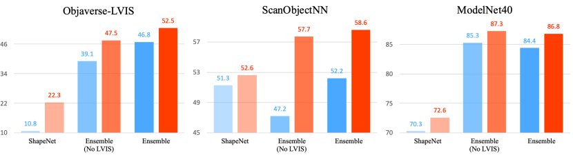
As illustrated in Figure 1, our MixCon3D consistently shows remarkable improvements over multiple popular 3D understanding benchmarks. For example, on the well-established ScanObjectNN dataset, our approach substantially outperforms the prior art by 6.4%, demonstrating the strong generalization ability of MixCon3D. Moreover, on the challenging 1,156-category Objaverse-LVIS dataset with long-tailed distribution, our MixCon3D attains an accuracy of 52.5%, surpassing the competing models by a significant margin of 5.7%. Lastly, by following OpenShape (Liu et al., 2023a) to employ the learned 3D features in the tasks of text to 3D shape retrieval and point cloud caption generation, we showcase our newly learned 3D embedding space is well aligned with CLIP image and text embedding space.
2 Related Works
3D Representation Learning.
Point-based methods, a prominent category of 3D representation learning, have garnered much attention for their simplicity, effectiveness, and efficiency. The pioneering work, PointNet (Qi et al., 2017a), models the inherent permutation invariance of points with point-wise feature extraction and max-pooling, enabling direct processing of unstructured point sets. PointNet++ (Qi et al., 2017b) enhances PointNet with a hierarchical network architecture to effectively capture local and global geometric cues. Building upon this foundation, the 3D community has witnessed the emergence of a plethora of point-based methods, with a particular focus on the design of effective local modules (Qian et al., 2021; Wang et al., 2019b; a; Thomas et al., 2019; Tatarchenko et al., 2018; Xu et al., 2018; Liu et al., 2019; Zhao et al., 2021). PointNext (Qian et al., 2022) explores an orthogonal direction, underscoring the pivotal role of training and scaling strategies in effective 3D representation learning.
Another line of work focuses on designing self-supervised learning techniques tailored for point cloud understanding. Early endeavors along this direction centered around the proposition of various low-level pretext tasks, including self-reconstruction (Achlioptas et al., 2018; Deng et al., 2018), distortion reconstruction (Sauder & Sievers, 2019; Mersch et al., 2022), and normal estimation (Rao et al., 2020). Recently, the remarkable success of self-supervised learning in the language and vision domain has prompted researchers in the 3D domain to adopt analogous self-supervised learning paradigms. PointContrast (Xie et al., 2020), for instance, leverages the concept of contrasting two views of the same point cloud to facilitate high-level scene understanding. PointBERT (Yu et al., 2022) and PointMAE (Pang et al., 2022), based on the idea of masked modeling, train an autoencoder to recover the masked portion of data with the unmasked part of the input.
Different from designing better 3D backbones or self-supervised learning pretext tasks, this paper focuses on improving multimodal contrastive learning for 3D open-world understanding.
CLIP for 3D open-world understanding.
By training on web-scale image-text pairs, CLIP (Radford et al., 2021) has revolutionized the area of visual representation learning via language supervision. The extraordinary zero-shot recognition performance of CLIP has found applications in a lot of domains, including zero-shot text-to-3D generation (Hong et al., 2022; Jain et al., 2022; Michel et al., 2022; Sanghi et al., 2022), zero-shot 3D segmentation or detection (Jatavallabhula et al., 2023; Ding et al., 2023; Yang et al., 2023; Lu et al., 2023), and 3D shape understanding (Zhang et al., 2022; Zhu et al., 2022; Xue et al., 2023a; b; Qi et al., 2023; Hegde et al., 2023; Lei et al., 2023; Zhou et al., 2023). The early exploration in leveraging CLIP for 3D shape understanding typically involves the projection of the original point cloud into depth maps, followed by the direct application of 2D CLIP on them (Zhang et al., 2022; Zhu et al., 2022). However, this approach suffers from information loss during projection while introducing extra latency. Additionally, the domain gap between the synthetically rendered depth maps and natural images could significantly hurt CLIP performance.
More recently, multiple works (Xue et al., 2023a; b; Liu et al., 2023a) propose to learn a unified embedding space for image, text, and point cloud, through training a 3D encoder aligned with CLIP image/text encoder. Our work follows this line of work but takes one step ahead to fully unleash the power of contrastive learning between image, text, point cloud triplets by 1) proposing an image + point cloud joint representation alignment mechanism, and 2) utilizing multi-view images for better point-image alignment.
3 MixCon3D
In Section 3.1, we first review the existing paradigm of image-text-3D contrastive training. More importantly, we further analyze and improve the existing training recipe, leading to a stronger baseline. Next, we propose a novel joint representation alignment mechanism (Section 3.2) with the integration of multi-view 2D images (Section 3.3), combining complementary information captured by 2D and 3D sensors for better aligning with text features.
3.1 Preliminary: Image-Text-3D Contrastive Learning
Optimization Objectives of Cross-modal Contrastive Learning.
By exploiting a massive amount of image-text pairs crawled from the web, the CLIP model (Radford et al., 2021) has demonstrated exceptional open-world image understanding capability. Typically, given batched image-text pairs and the image, text encoders , , the CLIP is trained to bring the representations of paired image and text data closer by the contrastive loss as follows:
| (1) |
where and are the normalized image and text features output by projection heads. and are image and text projection heads and is a learnable temperature.
As the scale of 3D datasets is relatively smaller, previous works (Xue et al., 2023a; b; Liu et al., 2023a; Zeng et al., 2023) have resorted to the pre-trained CLIP image and text embedding space for training a vanilla 3D model (including 3D encoder and projection head ) with open-world recognition ability. Since CLIP is pre-trained on a much larger data scale and is well aligned, its image model and text model are frozen during training. Specifically, given batched input image , text , and point cloud triplets (hence the name image-text-3D), the 3D model is trained to align the point cloud representation to the CLIP embedding space by and (each has the similar formulation of Equation 1). In this case, the optimization objective becomes:
| (2) |
Method Temperature Parameter Batchsize Learning Rate Schedule Warm up EMA ULIP Share 64 Cosine Decay ✓ ✗ OpenShape Share 200 Step Decay ✗ ✗ Improved Recipe Separate 2k Cosine Decay ✓ ✓
Revisiting Training Recipe.
It is known to the 3D community that a well-tuned training recipe can lead to a dramatic performance boost (Qian et al., 2022). Yet, despite its impressively promising performance, the training recipe of the image-text-3D contrastive learning paradigm is underexplored. Thus, before diving deep into our method, we first revisit the training recipe of ULIP (Xue et al., 2023a) and OpenShape (Liu et al., 2023a), identifying useful changes, as listed in Table 1:
-
•
Batchsize. Contrastive learning benefits significantly from a large batch size (Cherti et al., 2023; Radford et al., 2021). Nevertheless, the state-of-the-art model (Xue et al., 2023a) still adopts a small batchsize of 64. We note a medium batchsize of 2k strikes a good trade-off between different datasets; but further increasing it fails to provide further improvement, presumably because of the limited data scale and frozen CLIP encoders. We opt for a batchsize of 2k by default.
-
•
Learning rate schedule. Unlike ULIP, OpenShape adopts the step learning rate decay schedule without warmup. Yet, the CLIP utilizes the cosine learning rate schedule with warmup by default, a setting known to help better train an image model (He et al., 2019). We adopt the same setting as CLIP and find it leads to clear improvement.
-
•
Exponential moving average. During training, we observe the model performance steadily increase on the synthetic Objaverse-LVIS dataset, while fluctuating drastically on the real-scanned ScanObjectNN dataset, presumably due to the domain gap. We employ Exponential Moving Average (EMA) (Tarvainen & Valpola, 2017) to alleviate the fluctuation issue to stabilize training.
-
•
Separate temparature. Features from different modalities may have different distributions. Prior works (Xue et al., 2023a; Liu et al., 2023a) use a shared temperature parameter (Wu et al., 2018) to control the concentration level of multi-modal features. Differently, we hereby use separate temperature parameters for each modality.
Together, as shown in Table 3, our enhanced recipe substantially boosts the top-1 accuracy of OpenShape baseline by 3.3%, 3.6%, and 1.9% on Objaverse-LVIS, ScanObjectNN, and ModelNet40, respectively. Next, we introduce two enhancements designed for 3D contrastive learning.
3.2 Image-3D to text Joint Representation Alignment
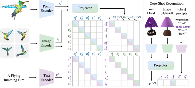
3D point cloud and 2D images are known to encode different yet complementary cues: point cloud better captures depth and geometry information, while images focus on catching dense semantic information (Bai et al., 2022; Liu et al., 2023b; Chen et al., 2023; Wang et al., 2023). Intuitively, the fusion of information from these two modalities could more accurately represent the corresponding 3D object in the real world and thus is expected to align better with the text modality. To this end, we introduce a simple yet effective image-3D to text joint representation alignment approach, which constructs a new 3D object-level representation by aggregating the respective features extracted from RGB image and point cloud modalities. On top of the contrast between the conventional tri-modal features with each other, the joint representation will also be aligned with text features via an additional contrastive loss.
Training Objectives.
Given batched data triplets and image-text-3D models (, , ), the corresponding features are denoted as vectors , , ), respectively. To model the joint representation, we concatenate the image features and point cloud features (i.e., ), and use a fully connected layer to project the joint representation . The extra contrastive term is:
| (3) |
where is the temperature parameter. In this case, the overall objective becomes:
| (4) |
where is the input image-text-point cloud data triplet. Note that we keep the conventional point cloud to text loss , enabling the model to make predictions solely based on 3D input even when corresponding images are unavailable (Uy et al., 2019; Wu et al., 2015). Additionally, different from ULIP and OpenShape, we retain the CLIP loss with an additional learnable projection head upon the frozen CLIP encoder.
Zero-Shot Inference.
The texts of class labels in the downstream tasks are used to connect to the learned 3D representation from the point cloud encoder, enabling the ability of zero-shot recognition. Specifically, the class text features are obtained by inputting the class label to the text encoder with prompt engineering. Then, for single and mixture modality inference, given the trained projector and extracted image , point cloud features, the logits , , between the 3D object and texts are calculated in different ways as follows:
| (5) |
3.3 Synergy with the Multi-view Mechanism
In the 3D world, a single-view image only contains limited information captured from a specific camera pose with an angle. Instead, multi-view, a prominent property in 3D representation, has demonstrated promising effectiveness in 3D understanding tasks (Su et al., 2015; Jaritz et al., 2019; Hamdi et al., 2021; 2023). Though previous works (Xue et al., 2023a; b; Liu et al., 2023a) render images from multiple viewpoints of the same point cloud when creating the data triplets, they merely sample one image from the rendered multi-view images when extracting the image features, which inherently encode only partial facets of the 3D object. In MixCon3D, we capitalize on the features accumulated from multi-view images to achieve a more holistic view of a 3D object.
Specifically, given multi-view images , which corresponds to the text description and point cloud , we replace the single-view image feature with the fusion of individual image features extracted from images . For example, given a fusion function (e.g., view-pooling (Su et al., 2015), maxpooling or MLP), the multi-view image feature is obtained by fusing the features of every single image , as .
4 Experiments
We first introduce our experimental setup in Section 4.1. Then, we compare previous state-of-the-art methods in Section 4.2. We also conduct a series of analysis on the key components (Section 4.3), including the improved training strategies, contrastive loss, multi-view, and effect of inference ways. Additionally, we establish the applicability of 3D representation learned by MixCon3D in the cross-modal applications such as text to 3D object retrieval and point cloud captioning (Section 4.4).
4.1 Experimental Setup
Pre-training datasets.
Following OpenShape (Liu et al., 2023a), the full pre-training dataset (denoted as “Ensemble”) contains four pieces: ShapeNet (Chang et al., 2015), 3D-FUTURE (Fu et al., 2021), ABO (Collins et al., 2022)) and Objaverse (Deitke et al., 2023). The point cloud is obtained by sampling 10,000 points from the mesh surface and the color is interpolated based on the mesh textures. The images are rendered from 12 preset camera poses that cover the whole object uniformly. Then, the paired texts are generated by BLIP (Li et al., 2022; 2023) and Azure cognition services with GPT4 (OpenAI, 2023) to filter out noisy text. In addition, we verify the effectiveness of our method trained by the ShapeNet dataset only and the ensembled dataset except for the LVIS (Gupta et al., 2019) categories (denoted as “Ensemble (No LVIS)”).
Down-stream datasets.
Three datasets are used for evaluating zero-shot point cloud recognition:
-
•
ModelNet40 (Wu et al., 2015) is a synthetic dataset comprising 3D CAD models, including 9,843 training samples and 2,468 testing samples, distributed across 40 categories.
-
•
ScanObjectNN (Uy et al., 2019) is a dataset composed of 3D objects acquired through real-world scanning techniques, encompassing a total of 2,902 objects that are systematically categorized into 15 distinct categories. We follow (Xue et al., 2023a; b; Liu et al., 2023a) and use the variants provided by (Yu et al., 2022) in our experiments.
- •
Implementation details.
We implement our approach in PyTorch (Paszke et al., 2019) and train the models on a server with 8 NVIDIA A5000 GPUs with a batch size of 2048. We train the model for 200 epochs with the AdamW (Loshchilov & Hutter, 2018) optimizer, a warmup epoch of 10, and a cosine learning rate decay schedule (Loshchilov & Hutter, 2016). The base learning rate is set to 1e-3, based on the linear learning rate scaling rule (Goyal et al., 2017): batchsize / 256. The EMA factor is set to 0.9995. Following Liu et al. (2023a), OpenCLIP ViT-bigG-14 (Cherti et al., 2023) is adopted as the pretrained CLIP model.
Method Encoder Training data Objaverse-LVIS ScanObjectNN ModelNet40 Top1 Top1-C Top3 Top5 Top1 Top1-C Top3 Top5 Top1 Top1-C Top3 Top5 PointCLIP - Depth inference 1.9 - 4.1 5.8 10.5 - 20.8 30.6 19.3 - 28.6 34.8 PointCLIP v2 - 4.7 - 9.5 12.9 42.2 - 63.3 74.5 63.6 - 77.9 85.0 ReCon - ShapeNet 1.1 - 2.7 3.7 61.2 - 73.9 78.1 42.3 - 62.5 75.6 CG3D - 5.0 - 9.5 11.6 42.5 - 57.3 60.8 48.7 - 60.7 66.5 CLIP2Point - 2.7 - 5.8 81.2 25.5 - 44.6 59.4 49.5 - 71.3 81.2 ULIP PointBERT 6.2 - 13.6 17.9 51.5 - 71.1 80.2 60.4 - 79.0 84.4 OpenShape SparseConv 11.6 - 21.8 27.1 52.7 - 72.7 83.6 72.9 - 87.2 93.0 MixCon3D SparseConv 23.5 17.5 40.2 47.1 54.4 56.1 73.9 83.3 73.9 70.2 88.2 94.0 OpenShape PointBERT 10.8 - 20.2 25.0 51.3 - 69.4 78.4 70.3 - 86.9 91.3 MixCon3D PointBERT 22.3 16.2 37.5 44.3 52.6 52.1 69.9 78.7 72.6 68.2 87.1 91.3 ULIP PointBERT Ensemble (No LVIS) 21.4 - 38.1 46.0 46.0 - 66.1 76.4 71.4 - 84.4 89.2 OpenShape SparseConv 37.0 - 58.4 66.9 54.9 - 76.8 87.0 82.6 - 95.0 97.5 MixCon3D SparseConv 45.7 33.5 67.0 73.2 56.5 60.5 77.8 87.5 83.3 82.4 95.6 97.6 OpenShape PointBERT 39.1 - 60.8 68.9 47.2 - 72.4 84.7 85.3 - 96.2 97.4 MixCon3D PointBERT 47.5 34.6 69.0 76.2 57.7 61.5 80.7 89.8 87.3 86.7 96.8 98.1 ULIP PointBERT Ensemble 26.8 - 44.8 52.6 51.6 - 72.5 82.3 75.1 - 88.1 93.2 OpenShape SparseConv 43.4 - 64.8 72.4 56.7 - 78.9 88.6 83.4 - 95.6 97.8 MixCon3D SparseConv 47.3 35.0 68.7 76.1 57.1 61.2 79.2 88.9 83.9 83.2 95.9 98.0 OpenShape PointBERT 46.8 34.0 69.1 77.0 52.2 53.2 79.7 88.7 84.4 84.9 96.5 98.0 MixCon3D PointBERT 52.5 38.8 74.5 81.2 58.6 62.3 80.3 89.2 86.8 86.8 96.9 98.3
4.2 Main Results
In Table 2, we compare the performance of our MixCon3D with state-of-the-art competitors across two representative encoders, SparseConv (Choy et al., 2019) and PointBERT (Yu et al., 2022); three different training set, “ShapeNet”, “Ensemble (No LVIS)”, and “Ensemble”; and three popular 3D recognition benchmarks, Objaverse-LVIS, ScanObjectNN, and ModelNet40.
We observe that our MixCon3D consistently exhibits superior performance on different scales of the dataset (From “ShapeNet” to “Ensemble” and types of 3D encoders (SparseConv and PointBERT)). Specifically, on the challenging long-tailed benchmark Objaverse-LVIS, MixCon3D greatly improves the zero-shot Top1 accuracy from 46.8% of OpenShape to 52.5% with PointBERT encoder and “Ensemble” training data. In addition, when tested on the ScanObjectNN dataset that comprises scanned points of real objects and thus a bigger domain gap (Uy et al., 2019), our MixCon3D also achieves a significant performance boost of 6.4% (58.6% vs.52.2%). These results altogether validate the effectiveness of our proposed MixCon3D, demonstrating a more powerful open-world 3D understanding ability.
4.3 Ablation Studies
Improved training recipe.
We show the effect of improved training strategies in Table 3. The separate temperatures obtain a notable performance improvement (+ 0.8% Top1 on ScanObjectNN), indicating the necessity of using separate dynamic scales of logits. A larger batchsize benefits image-text-3D contrastive pre-training, significantly increasing 1.2%/0.7% Top1 accuracy on Objaverse-LVIS and ScanObjectNN. We observe a similar effect of the cosine learning rate schedule with warmup, achieving 48.5% Top1 and 36.0% Top1-C on Objaverse-LVIS without any additional training cost. Lastly, the exponential moving average update brings consistent improvement, especially on the ScanObjectNN (+ 1.5%) with a larger domain gap.
MixCon3D component.
In Table 4, we analyze the effect of each critical component in MixCon3D. Interestingly, we find that the image-text alignment alone even leads to worse performance compared to the baseline (decreasing from 49.8% to 48.7% on Objaverse-LVIS and 86.1% to 84.7% on ModelNet40), which potentially hurts the alignment effectiveness on and . By contrast, our proposed image-3D to text joint alignment loss itself brings a considerable performance boost of at least 1.8% on all three datasets, and combining leads to further improvement. This clearly shows the paramount importance of aggregating complimentary useful cues in contrastive learning with image, point cloud, and text. Moreover, we adopt multi-view images to construct a more comprehensive representation of the 3D object on image modality and result in a further improvement of 0.9% and 0.5% Top1 on Objaverse-LVIS and ScanObjectNN, suggesting the importance of considering the holism of 3D objects on cross-modal alignment.
Multi-view component.
We next analyze the effect of fusion function (Table 5(a)) and the number of views (Table 5(b)) used during the pre-training. For , compared with the max poling operation, we observe that simply adopting view-pooling achieves promising improvement (52.5% v.s. 52.1% Top1 on Objaverse-LVIS). Adding an additional fully connected layer (FC) after the pooling operation may boost the performance on in-distribution Objaverse-LVIS (+ 0.2% Top1) while severely lowering the generalization ability on ScanObjectNN (- 6.2% Top1). Since the image modality is only accessible when testing on Objaverse-LVIS, increasing the number of views during training obtains a consistent improvement (from 51.6% to 53.2% Top1 and 38.2% to 39.5% Top1-C) but may slightly hurt the performance on ScanObjectNN (decreasing 0.5% Top1 when increasing the number of views from 4 to 8). To keep a trade-off between datasets, we choose the view-pooling as and view amount by default.
| Improvements | Objaverse-LVIS | ScanObjectNN | ModelNet40 | |||||||||
| Top1 | Top1-C | Top3 | Top5 | Top1 | Top1-C | Top3 | Top5 | Top1 | Top1-C | Top3 | Top5 | |
| Baseline | 46.5 | 34.0 | 69.0 | 76.8 | 52.0 | 53.2 | 77.5 | 87.5 | 84.2 | 84.9 | 95.9 | 97.4 |
| + Separate Temperature | 46.8 | 34.4 | 69.2 | 77.1 | 52.8 | 54.0 | 77.6 | 87.4 | 84.4 | 84.6 | 96.1 | 97.4 |
| + Large Batchsize | 48.0 | 35.3 | 70.1 | 77.4 | 53.5 | 55.5 | 78.0 | 87.7 | 84.8 | 85.3 | 96.4 | 97.7 |
| + LR Schedule | 48.5 | 36.0 | 70.6 | 77.7 | 54.1 | 56.3 | 78.2 | 87.9 | 85.0 | 85.0 | 96.4 | 97.9 |
| + EMA | 49.8 | 36.9 | 71.7 | 78.7 | 55.6 | 58.9 | 79.3 | 88.6 | 86.1 | 86.2 | 96.8 | 98.3 |
| Multi- View | Objaverse-LVIS | ScanObjectNN | ModelNet40 | |||||||||||
| Top1 | Top1-C | Top3 | Top5 | Top1 | Top1-C | Top3 | Top5 | Top1 | Top1-C | Top3 | Top5 | |||
| ✗ | ✗ | ✗ | 49.8 | 36.9 | 71.7 | 78.7 | 55.6 | 58.9 | 79.3 | 88.6 | 86.1 | 86.2 | 96.8 | 98.3 |
| ✓ | ✗ | ✗ | 48.7 | 36.2 | 70.4 | 77.7 | 55.4 | 59.7 | 75.8 | 85.6 | 84.7 | 84.8 | 96.6 | 97.9 |
| ✗ | ✓ | ✗ | 51.0 | 37.8 | 73.2 | 79.5 | 57.9 | 61.4 | 79.8 | 89.3 | 86.5 | 86.4 | 96.6 | 98.0 |
| ✓ | ✓ | ✗ | 51.6 | 38.2 | 73.7 | 80.6 | 58.1 | 61.9 | 80.3 | 89.2 | 86.6 | 86.6 | 96.4 | 98.1 |
| ✓ | ✓ | ✓ | 52.5 | 38.8 | 74.5 | 81.2 | 58.6 | 62.3 | 80.3 | 89.2 | 86.8 | 86.8 | 96.9 | 98.3 |
| Function | O-LVIS | S-Object | ||
| Top1 | Top1-C | Top1 | Top1-C | |
| - | 51.6 | 38.2 | 58.1 | 61.9 |
| View-pooling | 52.5 | 38.8 | 58.6 | 62.3 |
| View-pooling + FC | 52.7 | 39.1 | 52.4 | 54.1 |
| Max pooling | 52.1 | 38.4 | 56.7 | 60.0 |
| Max pooling + FC | 51.6 | 38.0 | 55.8 | 58.7 |
| Multi-View | O-LVIS | S-Object | ||
| Top1 | Top1-C | Top1 | Top1-C | |
| 1 | 51.6 | 38.2 | 58.1 | 61.9 |
| 2 | 52.3 | 38.9 | 57.0 | 60.5 |
| 4 | 52.5 | 38.8 | 58.6 | 62.3 |
| 8 | 52.7 | 39.3 | 58.1 | 61.7 |
| 12 | 53.2 | 39.5 | 54.2 | 56.1 |
| Point Cloud | Image | Multi- View | Objaverse-LVIS | |||
| Top1 | Top1-C | Top3 | Top5 | |||
| ✓ | ✗ | - | 50.4 | 37.4 | 72.2 | 79.1 |
| ✗ | ✓ | - | 44.5 | 34.5 | 64.2 | 70.6 |
| ✗ | ✓ | ✓ | 51.9 | 38.5 | 73.1 | 79.4 |
| ✓ | ✓ | - | 51.6 | 37.6 | 73.4 | 80.1 |
| ✓ | ✓ | ✓ | 52.5 | 38.8 | 74.5 | 81.2 |
Multi-modal Inference.
The introduction of joint alignment and multi-view images leads to a lot of inference options. For instance, whether we should use point cloud input alone, or combine point cloud with image input. Also, it is necessary to decide whether to apply single-view or multi-view images for complete coverage. We ablate a series of inference ways that aggregate different representations and show the results in Table 5(c). Even with multi-view images, simply using the point cloud (50.4% Top1) or image modality (51.6% Top1) obtains sub-optimal solutions (compared to 52.5% Top1 that uses modality fusion) since both only cover partial information of a 3D instance. As can be seen, the way of point cloud and image representation fusion, plus multi-view image feature extraction (achieving 52.5% Top1 and 38.8% Top1-C), surpasses all other options by a clear margin, underpinning the significance of knowledge aggregation from different representations.
4.4 Cross-modal Applications
To test how well the point cloud representation of our MixCon3D is aligned with CLIP pre-trained representations, we evaluate the learned representations on the following cross-modal tasks, following the practice in Liu et al. (2023a).
Text to 3D object retrieval.
We use cosine similarity between text embeddings of a specific input and 3D shape embeddings from the ensembled dataset as the ranking metric. We compare the retrieval result of our MixCon3D with that of OpenShape. As shown in Figure 3, our MixCon3D can capture more comprehensive feature representation, e.g., allowing for more accurate indexing such as the hummingbird and fine-grained retrieval in situations where the “lamp” is required to have an “electric wire”.
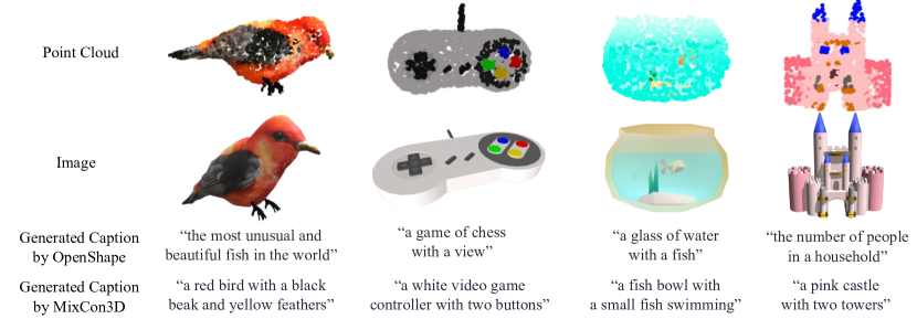
Point cloud captioning.
We feed the 3D shape embeddings of our MixCon3D into an off-the-shelf image captioning model ClipCap (Mokady et al., 2021), and compare the results with that of OpenShape. As can be observed in Figure 4, our MixCon3D captures a better 3D shape representation, thereby enhancing the generative model’s ability to generate more accurate and comprehensive captions.

5 Conclusion
In this paper, we present MixCon3D, a simple yet effective image-text-3D contrastive learning approach, which synergizes multi-modal joint alignment and multi-view representations for better open-world 3D understanding capability. Specifically, we propose constructing a simple yet effective image-3D to text joint representation alignment training scheme and capitalize on the features accumulated from multi-view images. In addition, we provide the first detailed training guideline in the field of image-text-3D contrastive learning. Together with the improved training pipeline, MixCon3D achieves not only superior performance on a wide range of 3D recognition benchmarks but also facilitates downstream cross-modal applications such as text-to-3D object retrieval and point cloud captioning. We hope our work could encourage more research endeavors to build the next-generation open-world 3D model.
Acknowledgement
This work is partially supported by TPU Research Cloud (TRC) program and Google Cloud Research Credits program.
References
- Achlioptas et al. (2018) Panos Achlioptas, Olga Diamanti, Ioannis Mitliagkas, and Leonidas Guibas. Learning representations and generative models for 3d point clouds. In International conference on machine learning, pp. 40–49. PMLR, 2018.
- Bai et al. (2022) Xuyang Bai, Zeyu Hu, Xinge Zhu, Qingqiu Huang, Yilun Chen, Hongbo Fu, and Chiew-Lan Tai. Transfusion: Robust lidar-camera fusion for 3d object detection with transformers. In Proceedings of the IEEE/CVF conference on computer vision and pattern recognition, pp. 1090–1099, 2022.
- Chang et al. (2015) Angel X Chang, Thomas Funkhouser, Leonidas Guibas, Pat Hanrahan, Qixing Huang, Zimo Li, Silvio Savarese, Manolis Savva, Shuran Song, Hao Su, et al. Shapenet: An information-rich 3d model repository. arXiv preprint arXiv:1512.03012, 2015.
- Chen et al. (2023) Zehui Chen, Zhenyu Li, Shiquan Zhang, Liangji Fang, Qinhong Jiang, and Feng Zhao. BEVDistill: Cross-modal BEV distillation for multi-view 3d object detection. In The Eleventh International Conference on Learning Representations, 2023.
- Cherti et al. (2023) Mehdi Cherti, Romain Beaumont, Ross Wightman, Mitchell Wortsman, Gabriel Ilharco, Cade Gordon, Christoph Schuhmann, Ludwig Schmidt, and Jenia Jitsev. Reproducible scaling laws for contrastive language-image learning. In Proceedings of the IEEE/CVF Conference on Computer Vision and Pattern Recognition, pp. 2818–2829, 2023.
- Choy et al. (2019) Christopher Choy, JunYoung Gwak, and Silvio Savarese. 4d spatio-temporal convnets: Minkowski convolutional neural networks. In Proceedings of the IEEE/CVF conference on computer vision and pattern recognition, pp. 3075–3084, 2019.
- Collins et al. (2022) Jasmine Collins, Shubham Goel, Kenan Deng, Achleshwar Luthra, Leon Xu, Erhan Gundogdu, Xi Zhang, Tomas F Yago Vicente, Thomas Dideriksen, Himanshu Arora, et al. Abo: Dataset and benchmarks for real-world 3d object understanding. In Proceedings of the IEEE/CVF Conference on Computer Vision and Pattern Recognition, pp. 21126–21136, 2022.
- Deitke et al. (2023) Matt Deitke, Dustin Schwenk, Jordi Salvador, Luca Weihs, Oscar Michel, Eli VanderBilt, Ludwig Schmidt, Kiana Ehsani, Aniruddha Kembhavi, and Ali Farhadi. Objaverse: A universe of annotated 3d objects. In Proceedings of the IEEE/CVF Conference on Computer Vision and Pattern Recognition, pp. 13142–13153, 2023.
- Deng et al. (2018) Haowen Deng, Tolga Birdal, and Slobodan Ilic. Ppf-foldnet: Unsupervised learning of rotation invariant 3d local descriptors. In Proceedings of the European conference on computer vision (ECCV), pp. 602–618, 2018.
- Ding et al. (2023) Runyu Ding, Jihan Yang, Chuhui Xue, Wenqing Zhang, Song Bai, and Xiaojuan Qi. Pla: Language-driven open-vocabulary 3d scene understanding. In Proceedings of the IEEE/CVF Conference on Computer Vision and Pattern Recognition, pp. 7010–7019, 2023.
- Fu et al. (2021) Huan Fu, Rongfei Jia, Lin Gao, Mingming Gong, Binqiang Zhao, Steve Maybank, and Dacheng Tao. 3d-future: 3d furniture shape with texture. International Journal of Computer Vision, 129:3313–3337, 2021.
- Goyal et al. (2017) Priya Goyal, Piotr Dollár, Ross Girshick, Pieter Noordhuis, Lukasz Wesolowski, Aapo Kyrola, Andrew Tulloch, Yangqing Jia, and Kaiming He. Accurate, large minibatch sgd: Training imagenet in 1 hour. arXiv preprint arXiv:1706.02677, 2017.
- Gupta et al. (2019) Agrim Gupta, Piotr Dollar, and Ross Girshick. Lvis: A dataset for large vocabulary instance segmentation. In Proceedings of the IEEE/CVF conference on computer vision and pattern recognition, pp. 5356–5364, 2019.
- Hamdi et al. (2021) Abdullah Hamdi, Silvio Giancola, and Bernard Ghanem. Mvtn: Multi-view transformation network for 3d shape recognition. In Proceedings of the IEEE/CVF International Conference on Computer Vision, pp. 1–11, 2021.
- Hamdi et al. (2023) Abdullah Hamdi, Silvio Giancola, and Bernard Ghanem. Voint cloud: Multi-view point cloud representation for 3d understanding. In The Eleventh International Conference on Learning Representations, 2023.
- He et al. (2019) Tong He, Zhi Zhang, Hang Zhang, Zhongyue Zhang, Junyuan Xie, and Mu Li. Bag of tricks for image classification with convolutional neural networks. In Proceedings of the IEEE/CVF conference on computer vision and pattern recognition, pp. 558–567, 2019.
- Hegde et al. (2023) Deepti Hegde, Jeya Maria Jose Valanarasu, and Vishal M Patel. Clip goes 3d: Leveraging prompt tuning for language grounded 3d recognition. arXiv preprint arXiv:2303.11313, 2023.
- Hong et al. (2022) Fangzhou Hong, Mingyuan Zhang, Liang Pan, Zhongang Cai, Lei Yang, and Ziwei Liu. Avatarclip: zero-shot text-driven generation and animation of 3d avatars. ACM Transactions on Graphics (TOG), 41(4):1–19, 2022.
- Jain et al. (2022) Ajay Jain, Ben Mildenhall, Jonathan T Barron, Pieter Abbeel, and Ben Poole. Zero-shot text-guided object generation with dream fields. In Proceedings of the IEEE/CVF Conference on Computer Vision and Pattern Recognition, pp. 867–876, 2022.
- Jaritz et al. (2019) Maximilian Jaritz, Jiayuan Gu, and Hao Su. Multi-view pointnet for 3d scene understanding. In Proceedings of the IEEE/CVF International Conference on Computer Vision Workshops, pp. 0–0, 2019.
- Jatavallabhula et al. (2023) Krishna Murthy Jatavallabhula, Alihusein Kuwajerwala, Qiao Gu, Mohd Omama, Tao Chen, Alaa Maalouf, Shuang Li, Ganesh Subramanian Iyer, Soroush Saryazdi, Nikhil Varma Keetha, et al. Conceptfusion: Open-set multimodal 3d mapping. In ICRA2023 Workshop on Pretraining for Robotics (PT4R), 2023.
- Lai et al. (2022) Xin Lai, Jianhui Liu, Li Jiang, Liwei Wang, Hengshuang Zhao, Shu Liu, Xiaojuan Qi, and Jiaya Jia. Stratified transformer for 3d point cloud segmentation. In Proceedings of the IEEE/CVF Conference on Computer Vision and Pattern Recognition, pp. 8500–8509, 2022.
- Lei et al. (2023) Weixian Lei, Yixiao Ge, Jianfeng Zhang, Dylan Sun, Kun Yi, Ying Shan, and Mike Zheng Shou. Vit-lens: Towards omni-modal representations. arXiv preprint arXiv:2308.10185, 2023.
- Li et al. (2022) Junnan Li, Dongxu Li, Caiming Xiong, and Steven Hoi. Blip: Bootstrapping language-image pre-training for unified vision-language understanding and generation. In International Conference on Machine Learning, pp. 12888–12900. PMLR, 2022.
- Li et al. (2023) Junnan Li, Dongxu Li, Silvio Savarese, and Steven Hoi. Blip-2: Bootstrapping language-image pre-training with frozen image encoders and large language models. arXiv preprint arXiv:2301.12597, 2023.
- Liu et al. (2023a) Minghua Liu, Ruoxi Shi, Kaiming Kuang, Yinhao Zhu, Xuanlin Li, Shizhong Han, Hong Cai, Fatih Porikli, and Hao Su. Openshape: Scaling up 3d shape representation towards open-world understanding. arXiv preprint arXiv:2305.10764, 2023a.
- Liu et al. (2019) Yongcheng Liu, Bin Fan, Shiming Xiang, and Chunhong Pan. Relation-shape convolutional neural network for point cloud analysis. In Proceedings of the IEEE/CVF conference on computer vision and pattern recognition, pp. 8895–8904, 2019.
- Liu et al. (2023b) Zhijian Liu, Haotian Tang, Alexander Amini, Xinyu Yang, Huizi Mao, Daniela L Rus, and Song Han. Bevfusion: Multi-task multi-sensor fusion with unified bird’s-eye view representation. In 2023 IEEE International Conference on Robotics and Automation (ICRA), pp. 2774–2781. IEEE, 2023b.
- Loshchilov & Hutter (2016) Ilya Loshchilov and Frank Hutter. Sgdr: Stochastic gradient descent with warm restarts. In International Conference on Learning Representations, 2016.
- Loshchilov & Hutter (2018) Ilya Loshchilov and Frank Hutter. Decoupled weight decay regularization. In International Conference on Learning Representations, 2018.
- Lu et al. (2023) Yuheng Lu, Chenfeng Xu, Xiaobao Wei, Xiaodong Xie, Masayoshi Tomizuka, Kurt Keutzer, and Shanghang Zhang. Open-vocabulary point-cloud object detection without 3d annotation. In Proceedings of the IEEE/CVF Conference on Computer Vision and Pattern Recognition, pp. 1190–1199, 2023.
- Mersch et al. (2022) Benedikt Mersch, Xieyuanli Chen, Jens Behley, and Cyrill Stachniss. Self-supervised point cloud prediction using 3d spatio-temporal convolutional networks. In Conference on Robot Learning, pp. 1444–1454. PMLR, 2022.
- Michel et al. (2022) Oscar Michel, Roi Bar-On, Richard Liu, Sagie Benaim, and Rana Hanocka. Text2mesh: Text-driven neural stylization for meshes. In Proceedings of the IEEE/CVF Conference on Computer Vision and Pattern Recognition, pp. 13492–13502, 2022.
- Mokady et al. (2021) Ron Mokady, Amir Hertz, and Amit H Bermano. Clipcap: Clip prefix for image captioning. arXiv preprint arXiv:2111.09734, 2021.
- OpenAI (2023) OpenAI. Gpt-4 technical report. arXiv:2303.08774, 2023.
- Pang et al. (2022) Yatian Pang, Wenxiao Wang, Francis EH Tay, Wei Liu, Yonghong Tian, and Li Yuan. Masked autoencoders for point cloud self-supervised learning. In European conference on computer vision, pp. 604–621. Springer, 2022.
- Paszke et al. (2019) Adam Paszke, Sam Gross, Francisco Massa, Adam Lerer, James Bradbury, Gregory Chanan, Trevor Killeen, Zeming Lin, Natalia Gimelshein, Luca Antiga, et al. Pytorch: An imperative style, high-performance deep learning library. Advances in neural information processing systems, 32, 2019.
- Qi et al. (2017a) Charles R Qi, Hao Su, Kaichun Mo, and Leonidas J Guibas. Pointnet: Deep learning on point sets for 3d classification and segmentation. In Proceedings of the IEEE conference on computer vision and pattern recognition, pp. 652–660, 2017a.
- Qi et al. (2017b) Charles Ruizhongtai Qi, Li Yi, Hao Su, and Leonidas J Guibas. Pointnet++: Deep hierarchical feature learning on point sets in a metric space. Advances in neural information processing systems, 30, 2017b.
- Qi et al. (2023) Zekun Qi, Runpei Dong, Guofan Fan, Zheng Ge, Xiangyu Zhang, Kaisheng Ma, and Li Yi. Contrast with reconstruct: Contrastive 3d representation learning guided by generative pretraining. In International Conference on Machine Learning (ICML), 2023.
- Qian et al. (2021) Guocheng Qian, Abdulellah Abualshour, Guohao Li, Ali Thabet, and Bernard Ghanem. Pu-gcn: Point cloud upsampling using graph convolutional networks. In Proceedings of the IEEE/CVF Conference on Computer Vision and Pattern Recognition, pp. 11683–11692, 2021.
- Qian et al. (2022) Guocheng Qian, Yuchen Li, Houwen Peng, Jinjie Mai, Hasan Hammoud, Mohamed Elhoseiny, and Bernard Ghanem. Pointnext: Revisiting pointnet++ with improved training and scaling strategies. Advances in Neural Information Processing Systems, 35:23192–23204, 2022.
- Radford et al. (2021) Alec Radford, Jong Wook Kim, Chris Hallacy, Aditya Ramesh, Gabriel Goh, Sandhini Agarwal, Girish Sastry, Amanda Askell, Pamela Mishkin, Jack Clark, et al. Learning transferable visual models from natural language supervision. In International conference on machine learning, pp. 8748–8763. PMLR, 2021.
- Rao et al. (2020) Yongming Rao, Jiwen Lu, and Jie Zhou. Global-local bidirectional reasoning for unsupervised representation learning of 3d point clouds. In Proceedings of the IEEE/CVF Conference on Computer Vision and Pattern Recognition, pp. 5376–5385, 2020.
- Sanghi et al. (2022) Aditya Sanghi, Hang Chu, Joseph G Lambourne, Ye Wang, Chin-Yi Cheng, Marco Fumero, and Kamal Rahimi Malekshan. Clip-forge: Towards zero-shot text-to-shape generation. In Proceedings of the IEEE/CVF Conference on Computer Vision and Pattern Recognition, pp. 18603–18613, 2022.
- Sauder & Sievers (2019) Jonathan Sauder and Bjarne Sievers. Self-supervised deep learning on point clouds by reconstructing space. Advances in Neural Information Processing Systems, 32, 2019.
- Schuhmann et al. (2021) Christoph Schuhmann, Richard Vencu, Romain Beaumont, Robert Kaczmarczyk, Clayton Mullis, Aarush Katta, Theo Coombes, Jenia Jitsev, and Aran Komatsuzaki. Laion-400m: Open dataset of clip-filtered 400 million image-text pairs. arXiv preprint arXiv:2111.02114, 2021.
- Schuhmann et al. (2022) Christoph Schuhmann, Romain Beaumont, Richard Vencu, Cade Gordon, Ross Wightman, Mehdi Cherti, Theo Coombes, Aarush Katta, Clayton Mullis, Mitchell Wortsman, et al. Laion-5b: An open large-scale dataset for training next generation image-text models. Advances in Neural Information Processing Systems, 35:25278–25294, 2022.
- Su et al. (2015) Hang Su, Subhransu Maji, Evangelos Kalogerakis, and Erik Learned-Miller. Multi-view convolutional neural networks for 3d shape recognition. In Proceedings of the IEEE international conference on computer vision, pp. 945–953, 2015.
- Tarvainen & Valpola (2017) Antti Tarvainen and Harri Valpola. Mean teachers are better role models: Weight-averaged consistency targets improve semi-supervised deep learning results. Advances in neural information processing systems, 30, 2017.
- Tatarchenko et al. (2018) Maxim Tatarchenko, Jaesik Park, Vladlen Koltun, and Qian-Yi Zhou. Tangent convolutions for dense prediction in 3d. In Proceedings of the IEEE conference on computer vision and pattern recognition, pp. 3887–3896, 2018.
- Thomas et al. (2019) Hugues Thomas, Charles R Qi, Jean-Emmanuel Deschaud, Beatriz Marcotegui, François Goulette, and Leonidas J Guibas. Kpconv: Flexible and deformable convolution for point clouds. In Proceedings of the IEEE/CVF international conference on computer vision, pp. 6411–6420, 2019.
- Uy et al. (2019) Mikaela Angelina Uy, Quang-Hieu Pham, Binh-Son Hua, Thanh Nguyen, and Sai-Kit Yeung. Revisiting point cloud classification: A new benchmark dataset and classification model on real-world data. In Proceedings of the IEEE/CVF international conference on computer vision, pp. 1588–1597, 2019.
- Wang et al. (2019a) Lei Wang, Yuchun Huang, Yaolin Hou, Shenman Zhang, and Jie Shan. Graph attention convolution for point cloud semantic segmentation. In Proceedings of the IEEE/CVF conference on computer vision and pattern recognition, pp. 10296–10305, 2019a.
- Wang et al. (2019b) Yue Wang, Yongbin Sun, Ziwei Liu, Sanjay E Sarma, Michael M Bronstein, and Justin M Solomon. Dynamic graph cnn for learning on point clouds. ACM Transactions on Graphics (tog), 38(5):1–12, 2019b.
- Wang et al. (2023) Zeyu Wang, Dingwen Li, Chenxu Luo, Cihang Xie, and Xiaodong Yang. Distillbev: Boosting multi-camera 3d object detection with cross-modal knowledge distillation. In Proceedings of the IEEE/CVF International Conference on Computer Vision (ICCV), pp. 8637–8646, 2023.
- Wu et al. (2015) Zhirong Wu, Shuran Song, Aditya Khosla, Fisher Yu, Linguang Zhang, Xiaoou Tang, and Jianxiong Xiao. 3d shapenets: A deep representation for volumetric shapes. In Proceedings of the IEEE conference on computer vision and pattern recognition, pp. 1912–1920, 2015.
- Wu et al. (2018) Zhirong Wu, Yuanjun Xiong, Stella X Yu, and Dahua Lin. Unsupervised feature learning via non-parametric instance discrimination. In Proceedings of the IEEE conference on computer vision and pattern recognition, pp. 3733–3742, 2018.
- Xie et al. (2020) Saining Xie, Jiatao Gu, Demi Guo, Charles R Qi, Leonidas Guibas, and Or Litany. Pointcontrast: Unsupervised pre-training for 3d point cloud understanding. In Computer Vision–ECCV 2020: 16th European Conference, Glasgow, UK, August 23–28, 2020, Proceedings, Part III 16, pp. 574–591. Springer, 2020.
- Xu et al. (2018) Yifan Xu, Tianqi Fan, Mingye Xu, Long Zeng, and Yu Qiao. Spidercnn: Deep learning on point sets with parameterized convolutional filters. In Proceedings of the European conference on computer vision (ECCV), pp. 87–102, 2018.
- Xue et al. (2023a) Le Xue, Mingfei Gao, Chen Xing, Roberto Martín-Martín, Jiajun Wu, Caiming Xiong, Ran Xu, Juan Carlos Niebles, and Silvio Savarese. Ulip: Learning a unified representation of language, images, and point clouds for 3d understanding. In Proceedings of the IEEE/CVF Conference on Computer Vision and Pattern Recognition, pp. 1179–1189, 2023a.
- Xue et al. (2023b) Le Xue, Ning Yu, Shu Zhang, Junnan Li, Roberto Martín-Martín, Jiajun Wu, Caiming Xiong, Ran Xu, Juan Carlos Niebles, and Silvio Savarese. Ulip-2: Towards scalable multimodal pre-training for 3d understanding. arXiv preprint arXiv:2305.08275, 2023b.
- Yang et al. (2023) Jihan Yang, Runyu Ding, Zhe Wang, and Xiaojuan Qi. Regionplc: Regional point-language contrastive learning for open-world 3d scene understanding. arXiv preprint arXiv:2304.00962, 2023.
- Yu et al. (2022) Xumin Yu, Lulu Tang, Yongming Rao, Tiejun Huang, Jie Zhou, and Jiwen Lu. Point-bert: Pre-training 3d point cloud transformers with masked point modeling. In Proceedings of the IEEE/CVF Conference on Computer Vision and Pattern Recognition, pp. 19313–19322, 2022.
- Zeng et al. (2023) Yihan Zeng, Chenhan Jiang, Jiageng Mao, Jianhua Han, Chaoqiang Ye, Qingqiu Huang, Dit-Yan Yeung, Zhen Yang, Xiaodan Liang, and Hang Xu. Clip2: Contrastive language-image-point pretraining from real-world point cloud data. In Proceedings of the IEEE/CVF Conference on Computer Vision and Pattern Recognition, pp. 15244–15253, 2023.
- Zhang et al. (2022) Renrui Zhang, Ziyu Guo, Wei Zhang, Kunchang Li, Xupeng Miao, Bin Cui, Yu Qiao, Peng Gao, and Hongsheng Li. Pointclip: Point cloud understanding by clip. In Proceedings of the IEEE/CVF Conference on Computer Vision and Pattern Recognition, pp. 8552–8562, 2022.
- Zhao et al. (2021) Hengshuang Zhao, Li Jiang, Jiaya Jia, Philip HS Torr, and Vladlen Koltun. Point transformer. In Proceedings of the IEEE/CVF international conference on computer vision, pp. 16259–16268, 2021.
- Zhou et al. (2023) Junsheng Zhou, Jinsheng Wang, Baorui Ma, Yu-Shen Liu, Tiejun Huang, and Xinlong Wang. Uni3d: Exploring unified 3d representation at scale. arXiv preprint arXiv:2310.06773, 2023.
- Zhu et al. (2022) Xiangyang Zhu, Renrui Zhang, Bowei He, Ziyao Zeng, Shanghang Zhang, and Peng Gao. Pointclip v2: Adapting clip for powerful 3d open-world learning. arXiv preprint arXiv:2211.11682, 2022.
Appendix A Appendix
A.1 Details of the 3D encoder
The tokenization of point cloud.
PointBERT backbone.
Following OpenShape (Liu et al., 2023a), we scale up the Point-BERT (Yu et al., 2022) model. The hyperparameters for scaling up are shown in Table 6.
| # Parameters | # Layers | Width | # Heads | MLP Dim | # Patches | Patch Embed Dim |
| 13.3M | 6 | 512 | 8 | 1024 | 64 | 128 |
| 25.9M | 12 | 512 | 8 | 1024 | 128 | 128 |
| 32.3M | 12 | 512 | 8 | 1536 | 384 | 256 |
| Clamp | Temperature Setting | Objaverse-LVIS | ScanObjectNN | ModelNet40 | |||||||||
| Top1 | Top1-C | Top3 | Top5 | Top1 | Top1-C | Top3 | Top5 | Top1 | Top1-C | Top3 | Top5 | ||
| ✗ | Unified | 46.5 | 34.0 | 69.0 | 76.8 | 52.0 | 53.2 | 77.5 | 87.5 | 84.2 | 84.9 | 95.9 | 97.4 |
| ✓ | Unified | 46.5 | 34.1 | 69.0 | 76.8 | 52.2 | 53.3 | 77.5 | 87.7 | 84.4 | 84.9 | 96.0 | 97.6 |
| ✗ | Separate | 46.4 | 34.0 | 69.0 | 76.8 | 52.5 | 53.7 | 77.2 | 87.2 | 84.3 | 84.6 | 96.0 | 97.5 |
| ✓ | Separate | 46.8 | 34.4 | 69.2 | 77.1 | 52.8 | 54.0 | 77.6 | 87.4 | 84.4 | 84.6 | 96.1 | 97.4 |
| Para. | Batchsize | Objaverse-LVIS | ScanObjectNN | ModelNet40 | |||||||||
| Top1 | Top1-C | Top3 | Top5 | Top1 | Top1-C | Top3 | Top5 | Top1 | Top1-C | Top3 | Top5 | ||
| 32.3M | 256 | 47.0 | 34.9 | 69.2 | 76.9 | 50.2 | 52.6 | 77.9 | 87.5 | 85.0 | 85.2 | 96.4 | 97.4 |
| 512 | 47.7 | 36.1 | 69.8 | 77.2 | 49.9 | 52.1 | 75.7 | 85.5 | 84.6 | 84.6 | 95.8 | 97.1 | |
| 1024 | 49.1 | 36.9 | 70.9 | 78.1 | 52.1 | 55.0 | 76.0 | 85.9 | 83.3 | 83.7 | 96.8 | 98.3 | |
| 2048 | 49.6 | 37.4 | 71.1 | 78.3 | 53.2 | 55.0 | 75.3 | 85.7 | 84.6 | 83.7 | 95.2 | 96.9 | |
| 4096 | 49.6 | 37.9 | 70.9 | 78.1 | 52.7 | 54.1 | 76.1 | 85.3 | 83.7 | 82.3 | 96.1 | 97.7 | |
| 25.9M | 256 | 46.8 | 34.4 | 69.2 | 77.1 | 52.8 | 54.0 | 77.6 | 87.4 | 84.4 | 84.6 | 96.1 | 97.4 |
| 512 | 47.3 | 34.7 | 69.6 | 77.1 | 52.5 | 55.6 | 77.2 | 87.4 | 84.3 | 84.6 | 96.3 | 98.1 | |
| 1024 | 47.8 | 35.0 | 69.9 | 77.2 | 52.9 | 56.2 | 77.7 | 87.5 | 84.4 | 85.3 | 96.3 | 98.0 | |
| 2048 | 48.0 | 35.3 | 70.1 | 77.4 | 53.5 | 55.5 | 78.0 | 87.7 | 84.8 | 85.3 | 96.4 | 97.7 | |
| 4096 | 48.5 | 35.6 | 70.4 | 77.6 | 52.9 | 55.1 | 77.9 | 87.8 | 84.3 | 85.4 | 95.9 | 97.5 | |
| 13.3M | 512 | 45.2 | 33.7 | 66.7 | 74.5 | 54.7 | 56.6 | 77.3 | 87.0 | 83.7 | 83.7 | 94.7 | 96.8 |
| 1024 | 45.8 | 34.3 | 67.1 | 74.8 | 54.2 | 56.4 | 76.3 | 86.4 | 85.2 | 84.0 | 95.6 | 97.7 | |
| 2048 | 46.3 | 35.1 | 67.3 | 74.8 | 53.1 | 54.4 | 78.5 | 87.4 | 83.5 | 83.4 | 95.4 | 97.5 | |
A.2 More details and experimental results of the strong baseline
We begin with the baseline developed by Liu et al. (2023a) and use the “Ensemble” dataset for training. The temperature parameters for scaling the logit in two contrastive losses are unified, and the batchsize is 200. To simplify the analysis, we don’t use the “Hard Negative Mining” method utilized by OpenShape.
The setting of temperature for the contrastive loss.
The temperature controls the range of logits in the softmax function used in the contrastive loss (Radford et al., 2021). We first follow the CLIP, which initializes the learnable temperature parameter to 14.28 and clamps the value if it exceeds 100. In the image-text-3D alignment paradigm, the point cloud encoder is trained to align image and text modalities simultaneously. Intuitively, different modalities may have separately appropriate logit ranges. To this end, we verify the effect of temperature settings (a unified one used by two losses or two separate ones, each used by a loss) in Table 7 and choose “Clamp+Separate” by default.
The effect of batchsize for different model sizes
. We systematically investigate the effect of batchsize across model sizes in Table 8. From the results, increasing the model size or batchsize can obtain a better performance on Objaverse-LVIS whose distribution matches the training set very well. However, the results of the other two datasets are barely satisfactory, indicating the model’s generalization ability trained by “Ensemble” dataset still has much room to improve. Considering a good trade-off between datasets and training efficiency, we use a medium model size of “25.9M” and batchsize of 2k for all the following ablation studies by default.
Hyperparameter analysis of EMA decay rate
. We analyze the effect of the decay rate used in the Exponential-Moving-Average (EMA) update. From the results shown in Table 9, choosing the decay rate from the range “0.999” to “0.9999” all yield promising results. Based on the results from three datasets, we choose “0.9995” by default.
| Decay Rate | Objaverse-LVIS | ScanObjectNN | ModelNet40 | |||||||||
| Top1 | Top1-C | Top3 | Top5 | Top1 | Top1-C | Top3 | Top5 | Top1 | Top1-C | Top3 | Top5 | |
| w/o EMA | 48.5 | 36.0 | 70.6 | 77.7 | 54.1 | 56.3 | 78.2 | 87.9 | 85.0 | 85.0 | 96.4 | 97.9 |
| 0.99 | 49.2 | 36.5 | 71.1 | 78.3 | 54.8 | 57.1 | 78.9 | 88.2 | 85.7 | 85.9 | 96.8 | 98.4 |
| 0.999 | 49.3 | 36.5 | 71.2 | 78.3 | 55.3 | 58.3 | 79.4 | 88.8 | 86.4 | 86.3 | 96.9 | 98.4 |
| 0.9995 | 49.8 | 36.9 | 71.7 | 78.7 | 55.6 | 58.9 | 79.3 | 88.6 | 86.1 | 86.2 | 96.8 | 98.3 |
| 0.9999 | 50.1 | 37.0 | 71.3 | 78.6 | 55.4 | 58.5 | 78.9 | 88.4 | 85.7 | 85.3 | 96.9 | 98.2 |
| 0.99999 | 0.3 | 0.1 | 0.5 | 1.1 | 17.1 | 11.2 | 25.2 | 42.6 | 5.3 | 5.4 | 13.5 | 21.6 |
Training stability.
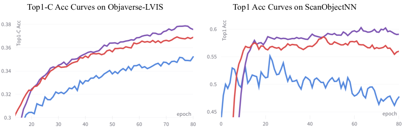
Empirically, we observe that the model’s test performance on the ScanObjectNN benchmark is unstable during training on the Objaverse dataset (the blue curve in Figure 5). Our improved baseline (the red curve) can significantly alleviate the training instability. Meanwhile, our proposed MixCon3D further boosts the performance for both the Objaverse-LVIS and ScanObjectNN.
| Inference Scheme | ||||||||||||||||
| Top1 | Top1-C | Top3 | Top5 | Top1 | Top1-C | Top3 | Top5 | Top1 | Top1-C | Top3 | Top5 | Top1 | Top1-C | Top3 | Top5 | |
| 51.1 | 37.9 | 73.2 | 80.0 | 50.4 | 37.4 | 72.2 | 79.1 | 51.1 | 38.4 | 73.1 | 79.8 | 51.5 | 39.4 | 73.7 | 80.5 | |
| 45.1 | 34.6 | 64.3 | 70.8 | 51.9 | 38.5 | 73.1 | 79.4 | 52.0 | 41.1 | 73.1 | 79.5 | 52.5 | 41.5 | 73.8 | 80.1 | |
| 51.6 | 38.2 | 73.7 | 80.6 | 52.5 | 38.8 | 74.5 | 81.2 | 52.8 | 39.1 | 74.7 | 81.5 | 53.2 | 39.5 | 75.4 | 82.1 | |
| 51.2 | 37.8 | 73.1 | 79.6 | 53.8 | 40.9 | 75.5 | 81.9 | 54.8 | 43.1 | 76.3 | 82.7 | 55.3 | 43.8 | 77.1 | 83.4 | |
A.3 Additional Experimental Results
Full results of Table 5(a) and Table 5(b).
We list the full results of using various types of , and view amounts in Table 11 and Table 12. Using simple view-pooling as obtains consistent improvement across three datasets. Adding an additional FC layer after the view-pooling or max pooling can enhance the Objaverse-LVIS performance while degrading the generalization ability on ScanObjectNN and ModelNet40. Given the availability of the image modality in the Objaverse-LVIS testing scenario, an increase in the number of views during the training phase yields a consistent enhancement in performance. However, this increment marginally impairs the efficacy of the ScanObjectNN and ModelNet40.
More results of Multi-Modal Inference
In Table 5(c), we analyze various multi-modal feature ensemble methods under four views (). To further analyze the combined impact of view amount and inference schemes, we perform in-depth analysis in Table 10, including individual modality inference (point cloud and image ) and modality ensemble inference (using to obtain and ). From the results, the ensemble scheme of the point cloud and the image modalities significantly improves performance. Moreover, benefitting from the large-scale pretrained CLIP model, the scheme further boosts the performance on Objaverse-LVIS when using multi-view images for inference.
| Function | Objaverse-LVIS | ScanObjectNN | ModelNet40 | |||||||||
| Top1 | Top1-C | Top3 | Top5 | Top1 | Top1-C | Top3 | Top5 | Top1 | Top1-C | Top3 | Top5 | |
| - | 51.6 | 38.2 | 73.7 | 80.6 | 58.1 | 61.9 | 80.3 | 89.2 | 86.6 | 86.6 | 96.4 | 98.1 |
| View-pooling | 52.5 | 38.8 | 74.5 | 81.2 | 58.6 | 62.3 | 80.3 | 89.2 | 86.8 | 86.8 | 96.9 | 98.3 |
| View-pooling + FC | 52.7 | 39.1 | 74.8 | 81.4 | 52.4 | 54.1 | 75.2 | 86.5 | 84.5 | 84.0 | 95.1 | 96.5 |
| Max pooling | 52.1 | 38.4 | 74.1 | 80.4 | 56.7 | 60.0 | 79.3 | 89.1 | 85.9 | 85.6 | 96.9 | 98.1 |
| Max pooling + FC | 51.6 | 38.0 | 73.2 | 80.3 | 55.8 | 58.7 | 77.1 | 87.6 | 85.2 | 85.6 | 96.0 | 97.6 |
| Multi-View | Objaverse-LVIS | ScanObjectNN | ModelNet40 | |||||||||
| Top1 | Top1-C | Top3 | Top5 | Top1 | Top1-C | Top3 | Top5 | Top1 | Top1-C | Top3 | Top5 | |
| 1 | 51.6 | 38.2 | 73.7 | 80.6 | 58.1 | 61.9 | 80.3 | 89.2 | 86.6 | 86.6 | 96.4 | 98.1 |
| 2 | 52.3 | 38.9 | 74.1 | 80.0 | 57.0 | 60.5 | 77.8 | 88.0 | 86.2 | 86.7 | 96.2 | 97.8 |
| 4 | 52.5 | 38.8 | 74.5 | 81.2 | 58.6 | 62.3 | 80.3 | 89.2 | 86.8 | 86.8 | 96.9 | 98.3 |
| 8 | 52.7 | 39.3 | 74.7 | 81.7 | 58.1 | 61.7 | 78.9 | 88.5 | 86.2 | 85.5 | 96.8 | 98.1 |
| 12 | 53.2 | 39.5 | 75.4 | 82.1 | 54.2 | 56.1 | 77.8 | 86.7 | 83.3 | 83.6 | 95.1 | 96.8 |