A high-performance surface acoustic wave sensing technique

Abstract

We present a superheterodyne-scheme demodulation system which can detect the amplitude and phaseshift of weak radio-frequency signals with extraordinarily high stability and resolution. As a demonstration, we introduce a process to measure the velocity of the surface acoustic wave using a delay-line device from 30 K to room temperature, which can resolve $\textless$ 0.1ppm velocity shift. Furthermore, we investigate the possibility of using this surface acoustic wave device as a calibration-free, high sensitivity and fast response thermometer.

The surface acoustic wave (SAW) is a special type of acoustic mode which propagates along the surface of a solid within a length scale of about its wavelength [1]. Environmental perturbations directly affect the propagation velocity $v$ and the insertion loss $\mit\Gamma$ of SAW. Therefore, SAW is broadly used as sensors in many applications with its unique advantages such as compact size, low cost and ease of fabrication [2, 3, 4]. In the past few decades, SAW sensors have been developed for various applications such as temperature [5, 6, 7], pressure [8, 9], strain [10], or for biosensing applications [11, 12]. SAW is also a very useful current-free technique in the study of quantum phenomena. It has been used to investigate the property of two dimensional system and prevail the nature of fragile quantum states [13, 14, 15, 16, 17, 18, 19, 20, 21].

In piezoelectric materials, the SAW traveling along the surface converts electric fields to mechanical motion and vice versa. It can be generated and detected by interdigital transducers (IDTs) when the frequency of applied/SAW-induced oscillating voltage matches the resonance condition $f_{r}=v/\lambda_{r}$, where $\lambda_{r}$ is the period of the IDT. The SAW velocity $v$ changes when the external physical properties such as temperature, pressure, etc. vary. SAW sensor devices can be categorized into two types. The first type is a resonator with the central IDT between two reflecting gratings that are totally reflecting at the desired resonance frequency $f_{r}$ [3, 6]. It is included into the feedback loop of an oscillator for frequency readout. The second type has a delay-line structure consisting of spatially separated emitter and receiver IDTs. The variation of the sensing region between the IDTs alters the phase $\mit\Phi$ of the received signal [13, 14, 15, 16, 17, 18, 19, 20, 21] or the resonance frequency $f_{r}$ of the device [7, 22, 10]. The resonator approach suffers from intrinsic electronics noise, parasitic oscillations and saturation of the oscillator [23]. In practice, the delay-line device is preferred for its better precision and reliability.

In this work, we introduce a superheterodyne-scheme radio frequency (RF) lock-in technique which can measure the phase ($\mit\Phi$) of a -90 dBm signal with sub-mrad resolution. We then demonstrate an application of SAW delay-line devices for temperature sensing and calibrate the SAW traveling time $\tau$ from $\sim$30 K to room temperature. At $\tau\simeq$ 1 $\mu$s and $f_{\text{r}}\simeq$ 560 MHz, we can detect $\sim$0.1-ppm of $\frac{\Delta\tau}{\tau}$, corresponding to $\sim 1$ mK temperature resolution at room temperature. Our setup with its combination of low excitation and high sensitivity shows potential to resolve very delicate responses of fragile quantum phases that are only visible at extremely low temperatures. In a separate work, we demonstrate such an application by studying quantum Hall states in a two dimensional system at mK temperature [24].

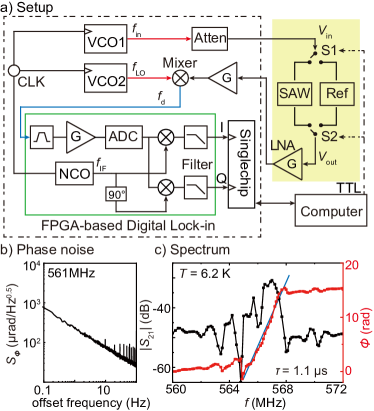
Figure 1: (a) Diagram of superheterodyne quadrature phase demodulation system. The FPGA-based digital lock-in module is shown in the green box. (b) Phase noise spectral density measured at room temperature. (c) The amplitude and phase of the SAW device measured by our setup as a function of frequency.

In order to measure the phase delay of our device, we develop a heterodyne-scheme lock-in technique that functions from 50 MHz to 1.5 GHz and has an exceptional phase noise performance. Fig. 1(a) shows a diagram of our setup. We use fractional phase locked-loops (PLL) to generate two single-frequency signals $V_{\text{in}}$ and $V_{\text{LO}}$, whose frequencies are locked to the reference clock frequency $f_{\text{CLK}}$ by $f_{\text{in}}$ (= $\frac{n}{m}\cdot f_{\text{CLK}}$) and $f_{\text{LO}}$ (= $\frac{n+k}{m}\cdot f_{\text{CLK}}$) respectively; $n$,$m$ and $k$ are integer values. $V_{\text{in}}$ is attenuated and sent to the device which attenuates the amplitude by $\mit\Gamma$ and introduces a phase delay $\mit\Phi$. The output signal of the device $V_{\text{out}}$ will be magnified by a broadband low noise amplifier (LNA) and then multiplied with $V_{\text{LO}}$ in the mixer. We then use a filter to extract the differential frequency component $f_{\text{d}}$ and digitize it with an audio-frequency A/D converter. We properly choose the internal Numerically Controlled Oscillator (NCO) module to generate the intermediate frequency (IF) at $f_{\text{IF}}=|f_{\text{in}}-f_{\text{LO}}|=\frac{k}{m}\cdot f_{\text{CLK}}$ and use it as the reference signal for the digital lock-in-type signal analysis of $V_{\text{d}}$. The amplitude of $V_{\text{d}}$ is proportional to $V_{\text{out}}$, and its phase shift $\mit\Phi_{\text{d}}$ from IF is offset from $\mit\Phi$ by a constant. In particular, we construct a reference channel with fixed attenuation and phase delay. Two microwave mechanical switches toggle between the device and reference channels to eliminate the constant phase offset and compensate for the drift of components such as amplifiers and mixers [10].

Our system is specifically optimised for the best phase stability and low-level RF signal, which is required in studying quantum physics [25, 24]. The superheterodyne-scheme downconverts the RF signal to intermediate frequency (IF) where quadrature demodulation is performed, thereby mitigating the 1/f noise [26]. We use two fractional phase locked loops (PLLs) to generate the measurement and reference signals, so that the phase stability is improved by the internal feedback loop in the PLLs [27]. In contrast to the high speed digitization used in many systems, our intermediate frequency is fixed at audio-frequency so that a low-noise A/D converter can be used and the high precision quadrature demodulation algorithm can be implemented. In addition, the phase noise from the clock-jittering can be eliminated by carefully matching the clocks used by PLLs, A/D converters and digital signal processors. Furthermore, the system features well-designed shielding between its various components and achieves an isolation of more than 80 dB between two channels. These precautions effectively reduce background noise and crosstalk interference.

In typical measurement conditions, the noise is almost always limited by the phase noise of the PLLs. The measured phase noise spectral density $S_{\phi}$(f), shown in Fig. 1(b), is proportional to $1/\sqrt{f}$ and equals about 0.2 mrad/$\sqrt{Hz}$ at 1 Hz. This corresponds to a bounded phase instability $\delta\mit\Phi$ of about 0.3 mrad. On the other hand, the input electronic noise floor is less than -160 dBm/Hz, leading to an equivalent phase noise spectral density lower than 0.3 mrad/$\sqrt{Hz}$ if the signal to be measured is above 1 pW (-90 dBm). For higher amplitude signals, the phase noise of PLLs dominates and limits the resolution [28, 29].

The above specifications are achieved by extremely careful design of radio frequency circuit, power and clock distribution, feedback temperature control of signal sources, as well as step-by-step shielding to meet the stringent requirement of ElectroMagnetic Compatibility (EMC) for over 80 dB channel isolation. Proper device selection is required. If the PLL is replaced by a commercial microwave signal generator (e. g. R$\&$S SMB100A), the phase noise is approximately -70 dBc/Hz at 1 Hz offset when the signal frequency is 1 GHz, comparable with our results 0.2 mrad/$\sqrt{Hz}$ at 1 Hz offset frequency shown in Fig. 1(b). However, the phase noise spectral density $S_{\phi}$(f) of our setup is proportional to 1/f down to 0.01 Hz, while the phase noise of typical microwave signal generator diverges at frequency below 1 Hz. The rapid increase of phase noise as offset frequency decreases suggests an unbounded drift of phase in hundreds of second, while our setup remains stable during the three day period of the data in Fig. 2(b). Our instrument focuses on long-term phase detection of small signals at a single frequency. Our typical resolution band width (RBW) is less than 0.3Hz, so that it can resolve signals lower than -160 dBm. This is 4 orders of magnitude lower than the about -120 dBm noise background of a commonly used vector network analyzer (e.g., Agilent Technologies E5071C). Furthermore, our homemade instrument has the same low noise background compared to commercial RF lock-in amplifiers (e.g., Zurich GHFLI), which implement an all-digital demodulation scheme. In summary, by sacrificing the flexibility, we achieve a very low noise background and extremely high long-term phase stability [24].

The device used in this demonstration is fabricated on an undoped bulk GaAs. We evaporate a 5-$\mu\text{m}$-period interdigital transducer (IDT) on each side of sample. 50 $\Omega$ resistors are connected in parallel to each IDT for broadband impedance matching. The SAW is generated at the emitter IDT by the input voltage $V_{\text{in}}$, propagates through the device and is captured by the receiver IDT on the opposite side of the sample as a voltage output $V_{\text{out}}$. We install the device in a dilution refrigerator and measure the attenuation and phase delay of $V_{\text{out}}$ using our lock-in setup. We can deduce the S-parameter $S_{21}$ with respect to $V_{\text{in}}$. Fig. 1(c) shows the $|S_{21}|$ and $\mit\Phi$ at different frequencies taken at 6.2 K. The $|S_{21}|$ peak indicates the resonance condition when the stimulated SAW wavelength $\lambda$ equals the IDT period $\lambda_{\text{r}}$. The $\simeq$2 MHz oscillations in $|S_{21}|$ are probably due to the echoes caused by the finite reflectivity of the two IDTs. The SAW traveling time from the emitter to the receiver IDTs can be measured by $\tau=\frac{1}{2\pi}d\mit\Phi/df=\frac{L}{\lambda}\cdot f_{\text{r}}^{-1}$, where $L$ is the nominal propagating distance. $N=\frac{L}{\lambda}$ is an integer defined by the lithography, i.e. the number of beats between the emitter and receiver if the frequency is close to $f_{\text{r}}$. We note that $\tau$ and $f_{\text{r}}$ remain almost unchanged when temperature is below 6.5 K. Therefore, we can deduce the device parameters at $T=0$ K to be ${}^{0}f_{r}=566.2$ MHz, ${}^{0}v=\lambda_{\text{r}}^{0}f_{\text{r}}=2830$ m/s, ${}^{0}\tau=1.1\mu$ s, $L=3.1$ mm and $N=620$.

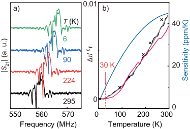
Figure 2: (a) $|S_{21}|$ of the device measured at different temperatures using Vector Network Analyzer. The traces are shifted vertically for clarity. (b) Black and pink curves present the temperature dependence of the propagation time shift $\Delta\tau/^{0}\tau$ measured by the phase approach (see text) using two different GaAs devices with 5 and 20$\mu$m IDT periods, respectively. The grey curve is the 3rd polynomial fitting of the 5$\mu$m period data. Black cross markers are deduced from the resonance frequency extracted from the data in Fig. 2(a) as verification for our method. Blue curve is the thermometer sensitivity ${}^{0}\tau^{-1}d\tau/dT$ derived from taking the derivative of the grey curve.

Besides using the resonance frequency, we can significantly improve the resolution of SAW velocity by directly measuring the propagation time from the phase delay (the phase approach). We choose a frequency $f\approx f_{\text{r}}$ so that the $|S_{21}|$ is close to its maximum. We then measure the phase $-\pi<\mit\Phi<\pi$, and calculate the corresponding delay time by $\tau=\frac{\mit\Phi}{2\pi f}+\frac{N}{f}$. Note that $\mit\Phi$ = 0 and $\tau=N\cdot f^{-1}$ if $f=f_{\text{r}}$, consistent with the mode where the SAW reflected from the receiver IDT constructively interferes with the emitting wave.

Our device can be used as a high resolution thermometer operating from below 30 K to above 300 K. Fig. 2(a) shows the $|S_{21}|$ taken by the Vector Network Analyzer at different temperatures, where the resonance frequency $f_{\text{r}}$ decreases as the temperature increases. The estimated thermal expansion $\Delta L/L$ is about two orders of magnitude smaller than the observed $\Delta f_{\text{r}}/f_{\text{r}}$, so that the SAW velocity change dominates this temperature-dependent shift and $\Delta f_{\text{r}}/^{0}f_{\text{r}}=\Delta v/^{0}v=-\Delta\tau/^{0}\tau$, where ${}^{0}f_{\text{r}}$, ${}^{0}v$ and ${}^{0}\tau$ are the resonance frequency, SAW velocity and propagation time at $T=0$ K. In Fig. 2(b), we summarize the $\Delta\tau/^{0}\tau$ deduced from the resonance frequency shift (symbols) and from our phase approach (curves). This $\Delta\tau/^{0}\tau$ vs. $T$ curve can be fitted as $\frac{\Delta\tau}{{}^{0}\tau}=(-0.8+2.6T+1.3*10^{-1}T^{2}-1.3*10^{-4}T^{3})$ [22]. Using this curve as a calibration, we can derive the temperature $T$ from the measured $\tau$. The sensitivity of the SAW thermometer, ${}^{0}\tau^{-1}d\tau/dT$ reaches about 40 ppm/K at room temperature and decreases to 10 ppm/K when the temperature drops to 30 K. The shrinkage of sensitivity limits the minimum operating temperature of the SAW thermometer.

The parameter $N$ is a well-defined integer by lithography and ${}^{0}v$ is an intrinsic parameter in high-purity materials such as GaAs. This allows us to use one calibration curve for different devices. The phase instability of our lock-in setup is sub-mrad, and the $\tau$ resolution is $N$-times enhanced by the delay-line structure. Therefore we can resolve $\tau$ as small as the $\frac{\delta\mit\Phi}{2\pi N}\sim$ 0.1ppm, leading to mK-level resolution at room temperature. It is worth mensioning that while a large $N$ leads to high resolution, it poses a restriction on the measurement frequency used in the phase approach, i.e. $f$ should be close to $f_{\text{r}}$ so that $N|f-f_{\text{r}}|/f_{\text{r}}<0.5$. An additional phase $2\pi[N|f-f_{\text{r}}|/f_{\text{r}}]$ should be added/subtracted to $\mit\Phi$, $[\cdot]$ means rounding algorithm, if the chosen $f$ is too far away from the resonance frequency $f_{\text{r}}$. Properly choosing the distance and period of the IDTs can compromise between the sensitivity and the ease of use.

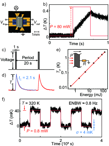
Figure 3: (a) The picture of our demonstration sensor device. (b) The time-domain response of temperature change using 10kHz sampling rates. The red trace is the heating power. (c & d) The pulsed heating voltage applied to the heater, and the measured temperature response of the SAW thermometer. The blue curve is the numerically simulated result. (e) Measured temperature peak $T_{\text{P}}$ as a function of heating energy per pulse. Inset is our model to describe the heating process. (f) Long-term measurement with a 1000-s-period, 0.8 mW amplitude square wave heating.

SAW sensors have an ultra-fast response to external environment, and measuring phase delay allows us to read the sensor response with minimal delay. In order to study the dynamic response of the SAW thermometer, we evaporate a platinum resistance wire (666 $\Omega$) as a heating element between the IDTs, see Fig. 3(a). The device is installed in a vacuum thermostat where the temperature is kept slightly above the room temperature at 320 K. We use $f=561.4$ MHz and -40 dBm RF input power so that the SAW heating is negligible. In Fig. 3(b), we apply an 80 mW, 0.3-second-wide square heating pulse and record the output at 10 kHz sampling rate. From the Fig. 2(b) curve, the measured phase $\mit\Phi$ is converted to temperature variation $\Delta T$ using a sensitivity $(2\pi N)^{-1}d\mit\Phi/dT\simeq$ 46 ppm/K. In Fig. 3(b), $\Delta T$ increases immediately when the heater is switched on, and we observe no delay of more than a few milliseconds.

We can describe the timeline of the thermal process for better understanding. The temperature at the device surface increases immediately when the current through the Pt wire generates heat. The heat defuses into the GaAs substrate which reaches a thermally steady state within a few milliseconds. The temperature sensor output responds as soon as the SAW reaches the receiver IDT after a propagation delay of 1 $\mu$s. In order to investigate this process, we apply 20-s-separated 1-s-wide heating pulses with different power. A typical measured response is shown in Fig. 3(d), and the peak height $T_{\text{P}}$ is summarized as a function of heating power for each pulse in Fig. 3(e). Each temperature peak in Fig. 3(d) has an exponential decay time $t_{\text{c}}\simeq 2.1$ s after each heating pulse. This decay time can be explained by the model shown in the inset of Fig. 3(e). Here the evolution of device temperature $T$ is described by the equation $P=C_{\text{D}}\cdot dT/dt-T/R$, where $P$ is the heating power, $C_{\text{D}}$ is the thermal capacitance of device and $R$ is the thermal resistance between the sensor and the heat sink. By linearly fitting $T_{\text{P}}$ and the energy of each pulse in Fig. 3(e), we can deduce the thermal capacitance of our device to be $C_{\text{D}}=53$ mJ/K. A more accurate estimate of $C_{\text{D}}$ is 42 mJ/K once the finite thermal resistance $R$ is taken in account. $R$ is estimated from the decay time as $R=t_{\text{c}}/C_{\text{D}}\simeq$ 50 mK/mW. The numerical simulation is shown by the blue curve in Fig. 3(d).

We can apply a constant heating power so that the device will reach a steady state determined by the finite $R$. In Fig. 3(f), we apply a 745 mV, 1000-second-period voltage to the heater, generating a heating power of 0.8 mW. We observe about 41 mK temperature increase of the sample when the heater is on, corresponding to a thermal resistance of $R=51$ mK/mW. This is consistent with the results of the pulsed heating measurement in Fig. 3(c-e). The standard deviation of $\Delta T$ in Fig. 3(f) is only 4 mK at 0.8 Hz measurement bandwidth, evidencing the exceptionally high performance of this proposed temperature sensor.

In conclusion, we introduce an approach to measure the propagation time of the SAW delay-line devices with 0.1-ppm resolution, and demonstrate that these devices show considerable promise for high-sensitivity and high-stability temperature sensors. This technique would be of interest for future applications due to its accuracy, sensitivity and fast response time.