Acousto-optic reconstruction of exterior sound field based on concentric circle sampling with circular harmonic expansion

Abstract

Acousto-optic sensing provides an alternative approach to traditional microphone arrays by shedding light on the interaction of light with an acoustic field. Sound field reconstruction is a fascinating and advanced technique used in acousto-optics sensing. Current challenges in sound-field reconstruction methods pertain to scenarios in which the sound source is located within the reconstruction area, known as the exterior problem. Existing reconstruction algorithms, primarily designed for interior scenarios, often exhibit suboptimal performance when applied to exterior cases. This paper introduces a novel technique for exterior sound-field reconstruction. The proposed method leverages concentric circle sampling and a two-dimensional exterior sound-field reconstruction approach based on circular harmonic extensions. To evaluate the efficacy of this approach, both numerical simulations and practical experiments are conducted. The results highlight the superior accuracy of the proposed method when compared to conventional reconstruction methods, all while utilizing a minimal amount of measured projection data.

I Introduction

Acousto-optics sensing methodologies utilize light as the principal sensing modality to non-intrusively sample acoustic fields within a given volume through a sparse array of optical measurements performed remotely. In contrast to conventional electromechanical transducers, acousto-optic methods do not yield localized acoustic pressure measurements due to the acousto-optic interaction taking place throughout the entire optical path [1]. Among numerous acousto-optic sensing methods developed so far [2], precision optical interferometry has played a central role in measuring audible sound, such as laser Doppler vibrometry [3, 4, 1], parallel phase-shifting interferometry and digital holography [5, 6, 7, 8, 9, 10, 11], and midfringe locked interferometry [12].

Computed tomography, frequently observed in medical imaging or nondestructive testing domains, enables the reconstruction of the spatial distribution of physical property from its projection measurements [13]. In acousto-optic sensing, the tomographic reconstruction of the sound field is essential to obtain sound pressure distributions from the measured laser projection data.

The most common tomographic reconstruction technique is filtered back-projection (FBP) [14]. Although this technique is simple and frequently employed [15, 1, 16, 17], the reconstruction accuracy may not be optimal for sound fields. Recently, physical model-based sound-field reconstruction methods have demonstrated their superiority over conventional FBP methods [18, 19, 20, 21] because they ensure that the reconstructed field satisfies the physical properties of sound. A typical reconstruction algorithm in the physical model-based group is the plane-wave expansion (PWE) [19, 21].

A challenge in the existing sound-field reconstruction methods is the so-called exterior problem where the sound source is located inside the reconstruction area. Fig. 1 illustrates the two sound-field reconstruction problems, the interior problem reconstructs the sound field inside a closed space (represented by a dashed line) where a sound source is located outside the space, whereas the exterior problem reconstructs the sound field outside a closed space where a sound source is located inside the space. Since the existing reconstruction algorithms are optimized for the interior reconstruction problem, they exhibit suboptimal performance for the exterior situation. Nevertheless, the reconstruction of the external sound field is a critical problem set that includes essential applications such as directivity measurement of sound sources and estimating the radiated sound field to an infinite region.

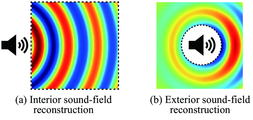
Figure 1: Illustration of (a) interior and (b) exterior sound-field reconstruction problems.

In this study, we present a novel exterior reconstruction method founded upon a concentric circle sampling scheme, utilizing circular harmonics as the expansion coefficients. To the best of our knowledge, this research represents the pioneering effort to facilitate the acousto-optic reconstruction of exterior sound fields, even in cases where the sound source is situated within the confines of the reconstruction area.

The rest of this paper is structured as follows: Section II introduces the proposed method comprising of concentric circle sampling technique and circular harmonic expansion of the sound field. Section III presents the simulation setups and the corresponding simulated results. This is followed by the exposition of the experiment setups and the actual experimental results. Section IV then meticulously presents and analyzes the experimental findings. Section V engages in relevant discussions to shed light on the implications of the results. Finally, Section V encapsulates the research with a conclusive summary of key findings and their broader significance.

II Proposed method

II-A Principle of acousto-optic sensing

In Fig. 2, an exemplification of the Laser Doppler Vibrometer (LDV) is presented, which serves to gauge acoustically induced phase shifts of light. The functioning of this apparatus involves the generation of a laser beam, subsequently bifurcated into two distinct branches: the sensing branch and the reference branch. The sensing beam is then directed through the sound field $p(r)$, wherein it undergoes backscattering upon interacting with the mirror surface and is eventually retrieved at the LDV optics system. The measurement principle can be found in the literature [1]. In short, the sensing beam experiences the phase modulation caused by sound due to the acousto-optic effect, which is detected by the LDV. A notable characteristic of this measurement method is that the detected signal is proportional to the line integral of sound pressure along the sensing beam.

II-B Concentric circular sampling

For exterior reconstruction problems, since a sound source should be located in the center part of the reconstruction area (as depicted in Fig. 1), sensing laser paths must avoid this part. Considering practical experimental implementation, we propose the concentric circle sampling scheme as shown in Fig. 3. The projections $S$ are sampled by laser beams surrounding the circle with radius $R$ and rotation $\phi$. This sampling scheme is easily achieved by rotating the sound source while keeping the laser beam fixed. In order to enhance the fidelity of reconstructed sound fields, it is possible to augment the acquisition of projections by incorporating numerous circles with varying radii, such as $R_{1}$, $R_{2}$, and $R_{3}$ as depicted in Fig. 3, or by employing smaller angular rotation increments. In this context, Fig. 3 illustrates a demonstration with a representation of 72 projections derived from a single concentric circle when the angular interval is 5^∘. This choice of the number of projections was made to strike a judicious balance between the quality of reconstruction and the computational complexity inherent in the reconstruction process. Another important factor to consider is the optimal number of concentric circles to use in sound field reconstruction. In an upcoming section, we will share initial findings and discuss this issue.

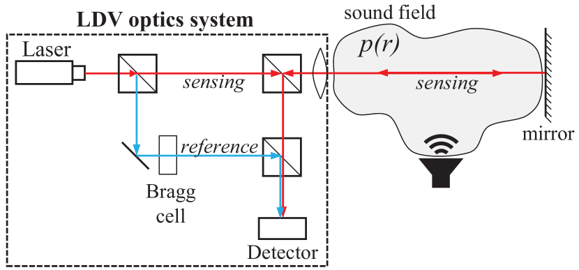
Figure 2: Acousto-optic sensing utilizing a Laser Doppler Vibrometer (LDV) device.

Figure 3: The proposed concentric circle sampling samples a sound field along the tangent line of a circle of radius $R_{i}$ at given angular intervals. The lines in the images represent measurement laser trajectories when the angular interval is 5^∘.

II-C Circular harmonic expansion of sound field

In this section, we expound upon the sound field reproduction technique employing circular harmonics, with a focus on the global exterior sound field as the area of interest. The acoustic field generated by an arbitrary sound source within a two-dimensional exterior space can be accurately depicted through the application of circular harmonic expansion (CHE), as exemplified in the work of E. G. Williams [22]. This representation can be expressed as follows:

$$p(r,\phi,\omega)=\sum\limits_{n=-\infty}^{\infty}{{a_{n}(\omega)}}{H_{n}^{(2)}}(kr){e^{jn\phi}},$$ (1)

where ${a_{n}(\omega)}$ represent the sound field coefficient for the order $n$ and ${H_{n}^{(2)}}\left(\cdot\right)$ is the Hankel function of the second kind. The symbols $\omega$ and $k$ correspond to the angular frequency and wave number, respectively, with the relationship between them given by $k=\omega/c$, where $c$ denotes the velocity of propagation.

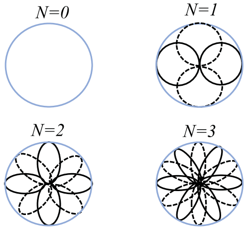
Figure 4: The polar coordinate representation of $e^{jn\phi}$, which serves as the foundational basis for circular harmonic expansion, is exemplified for $N$ values of 0, 1, 2, and 3.

Figure 4 shows the polar coordinate representation of $e^{jn\phi}$. Within our reconstruction method, the selection of the parameter $n$ was made in a flexible manner, contingent upon the specific frequency of the sound signal and the minimal radius of the concentric circle. This choice was crucial to ensure the comprehensive representation of the reconstructed sound field.

II-D Reconstruction algorithm

According to acousto-optic theorem and the circular harmonic expansion of the sound field, the projection $s_{m}$ can be written as

$${s_{m}}=\int{p(r,\phi,\omega)d{l_{m}}\approx\sum\limits_{n=-N}^{N}{{a_{n}}\int{{H_{n}^{(2)}}(kr){e^{jn\phi}}d{l_{m}}}}},$$ (2)

where $l_{m}$ represents the sensing laser trajectory of the $m$th measurement and the infinite sum of circular harmonics is truncated by order $N$. Equation (2) can be expressed algebraically as follows.

$$\mathbf{s}\approx\mathbf{H}\mathbf{a},$$ (3)

where $\mathbf{H}\in{\mathbb{C}^{M\times(2N+1)}}$ is a matrix with elements ${h_{m,n}}=\int{{H_{n}^{(2)}}(kr){e^{jn\phi}}d{l_{m}}}$. $\mathbf{a}\in{\mathbb{C}^{N}}$ are the expansion coefficients of the $N$ circular harmonic waves in the expansion. These coefficients can be determined through the regularized least squares method.

$$\mathbf{\tilde{a}}=\arg\mathop{\min}\limits_{\mathbf{a}\in{\mathbb{C}^{N}}}{\left\|\mathbf{a}\right\|_{2}}$$ (4)

subject to ${\left\|{\mathbf{s}-\mathbf{H}\mathbf{a}}\right\|_{2}}\leq\varepsilon$, where $\varepsilon$ is the permitted discrepancy between measurement $\mathbf{s}$ and $\mathbf{H}\mathbf{a}$. After obtaining the expansion coefficients $\mathbf{\tilde{a}}$, the reconstructed sound field is calculated as

$$\mathbf{\tilde{p}}=\mathbf{G}\mathbf{\tilde{a}}$$ (5)

where $\mathbf{\tilde{p}}\in{\mathbb{C}^{L}}$ denote estimated pressure at positions $r_{1},...,r_{L}$, and $\mathbf{G}\in{\mathbb{C}^{L\times(2N+1)}}$ includes elements ${g_{l,n}}=a_{n}{H_{n}^{(2)}}(kr_{l}){e^{jn\phi_{l}\cdot{r_{l}}}}$.

III Simulation

III-A Reference multi-source complex sound field

The 2D sound field generated by a point source is given as follows

$$p(x,y,k)=A\frac{i}{4}H_{0}^{(1)}(k\left|{r-{r_{0}}}\right|),$$ (6)

where $i=\sqrt{-1}$, $A$ is the amplitude of the sound field, $\left|{r-{r_{0}}}\right|=\sqrt{{{(x-{x_{0}})}^{2}}+{{(y-{y_{0}})}^{2}}}$ is the distance between $r$ and $r_{0}$. $r_{0}$ and $r$ are positions of a point source and position to calculate sound pressure, respectively. $k=\frac{{2\pi}}{\lambda}$ is the wavenumber of sound. $\lambda$ is the wavelength of sound, and $H_{0}^{(1)}(.)$ is the Hankel function of the first kind of order 0 [23].

As reference sound fields for simulating the exterior reconstruction problem, we generated sound fields within the area of 0.7 m $\times$ 0.7 m by the superposition of multiple point sources located within a circular area of minimum radius $R_{\mathrm{min}}=0.3\,$m. The generated reference sound fields are shown in the tops of Figs. 5 and 6, which are created from five sound sources at different phases and positions. The five sound sources have the phases of $\phi=\{\pi/6,2\pi/6,3\pi/6,4\pi/6,5\pi/6\}$ and located at $\{[0,0],[-0.05,0],[0,-0.05],[0.05,0],[0,0.05]\}$, respectively.

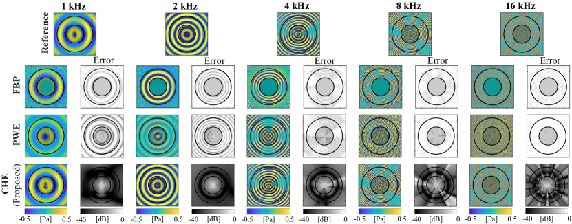
Figure 5: A comparative analysis was conducted on sound fields reconstructed by distinct reconstruction algorithms, namely FBP, PWE, and the proposed CHE. The reference sound fields were constructed using multiple sound point sources distributed in the proximity of a central location and across a range of frequencies.

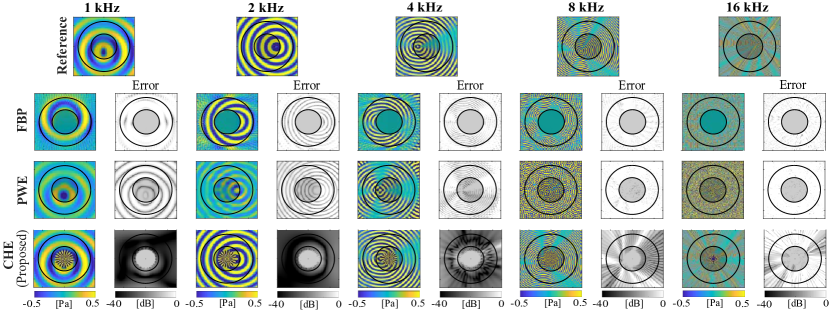
Figure 6: A comparative evaluation was conducted to assess the sound field reconstruction quality of various reconstruction algorithms, specifically FBP, PWE, and the proposed CHE. The reference sound fields were meticulously composed, featuring multiple sound point sources positioned at locations distanced from the central point. The specified locations for the groups of sound sources were as follows: at 1kHz: [0,0.12], 2 kHz: [0.2,0], 4 kHz: [-0.2,0], 8 kHz: [-0.2,0.1], and 16 kHz: [0.2,-0.1]. These sound fields were generated at distinct frequencies for the express purpose of evaluation.

III-B Simulated sound-field reconstruction

In order to assess the quality of the reconstructions, we used reconstruction error [24] which is calculated using $\varepsilon(r)=10{\log_{10}}\left\{{{{{{{{\left|{\tilde{p}(r)-p(r)}\right|}^{2}}}\mathord{\left/{\vphantom{{{{\left|{\tilde{p}(r)-p(r)}\right|}^{2}}}{\left|{p(r)}\right|}}}\right.\kern-1.2pt}{\left|{p(r)}\right|}}}^{2}}}\right\}$, where $\tilde{p}(r)$ and $p(r)$ are the reconstructed and reference sound pressure at position $r$, respectively. We computed the reconstruction error on a pixel-wise basis and juxtaposed the resulting error images alongside each corresponding reconstructed sound field solely for evaluative purposes. In order to enable a rigorous comparative analysis, we conducted simulations involving sound fields generated at different frequencies. For each frequency, we assessed two distinct scenarios wherein sound sources were positioned both at the center and off-center locations. To ensure equitable comparisons, we maintained a uniform number of projections (M = 2232) across three reconstruction algorithms: FBP, PWE, and the proposed CHE-based approach. In the case of the PWE method, our simulations entailed the use of 200 plane waves.

Figure 5 depicts the reconstructed sound fields utilizing three distinct methods: FBP, PWE, and CHE. These reconstructions were performed with the sound sources located at the central coordinates [0, 0]. We employed identical quantities of circular harmonics $N=15$ for sound fields at various frequencies: 1 kHz, 2 kHz, 4 kHz, 8 kHz, and 16 kHz. Examination of the reconstructed sound fields and accompanying reconstruction error images highlights certain noteworthy findings. Specifically, the PWE method exhibited difficulties in achieving accurate sound field reconstruction, while the FBP approach displayed suboptimal reconstruction quality. In contrast, the proposed CHE approach consistently yielded the highest quality reconstructions among the three methods under consideration.

Figure 6 illustrates the reconstruction outcomes in scenarios where sound sources are positioned at varying distances from the central location. In this particular scenario, the sound fields exhibit a greater degree of complexity, necessitating a larger number of circular harmonics compared to the scenario wherein the sound sources are situated at the center position. More specifically, we employed $N\,$=$\,20$ for sound fields at 1 kHz, 2 kHz, and 4 kHz, while for sound fields at 8 kHz and 16 kHz, we utilized $N=30$ and $N=40$ for the reconstruction process, respectively. The outcomes reveal that FBP and PWE exhibit suboptimal reconstruction performance within the frequency bands of 1 kHz, 2 kHz, and 4 kHz, characterized by either amplitude distortion or misalignment in the reproduced sound source positions when compared to the reference sound field. At higher frequency ranges, both FBP and PWE fail to effectively reconstruct the sound fields. Conversely, across all frequency ranges, the CHE-based method consistently delivers the highest reconstruction quality.

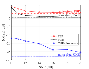
Figure 7: An evaluation is conducted to assess the quality of 2 kHz sound-field reconstruction achieved by three distinct reconstruction methods (namely, FBP, PWE, and proposed CHE) under the influence of AWGN at varying levels of signal-to-noise ratio (SNR).

To investigate the reconstruction performances against noise, different amounts of white Gaussian noises are added to the reference sound field of 2 kHz shown in Fig. 5, and the reconstruction errors among the three methods are compared. For comparing the overall errors across the entire reconstruction area, the following normalized mean square error (NMSE) in decibels (dB) is used; $\mathrm{NMS{E_{dB}}}=20{\log_{10}}({{{{\left\|{\tilde{p}-p}\right\|}_{2}}}\mathord{\left/{\vphantom{{{{\left\|{\tilde{p}-p}\right\|}_{2}}}{{{\left\|p\right\|}_{2}}}}}\right.\kern-1.2pt}{{{\left\|p\right\|}_{2}}}})$. Fig. 7 illustrates the comparison of NMSEs for the three methods. The findings illustrate the persistent supremacy of the proposed CHE algorithm in comparison to the FBP and PWE techniques across various noise levels. Significantly, the sound fields reconstructed by the FBP and PWE methods reach saturation points of NMSE at -1.3 dB, and -3.8 dB, respectively, when the SNR exceeds or equals 14. In contrast, the sound fields reconstructed by the proposed CHE algorithm consistently exhibit ongoing quality improvement as SNR increases, approaching sound field quality levels obtained in a noise-free environment, with an NMSE of -28.1 dB.

IV Experimental results

IV-A Experiment setup

TABLE I: Experiment settings

	Parameter	Value
Microphone	Type	Brüel Kjær 4939-A-011
Microphone amplifier	Type	BK NEXUS
	Signal delay	$\approx 10\,\mu$s
Loudspeaker	Type	Yamaha MS101III
Stage controller	Type	OptoSigma SHOT-302GS
	Movement step	10 mm
	Rotation step	5∘
LDV	Type	Polytec VibroFlex
	Decoder	Displacement
	Bandwidth	20 kHz
	Sensitivity	5 nm/V @M$\Omega$
	Range	10 nm
	Signal delay	900$\,\mu$s
Anechoic chamber	Temperature	16.9∘C
	Humidity	28.4 %
	Pressure	1000.4 hPa

Figure LABEL:fig:8a illustrates our experimental setup, while Fig. LABEL:fig:8b provides a view of the experimental setup within the anechoic chamber. The sound field was generated by a loudspeaker positioned laterally in relation to the LDV. Instead of adjusting the position and angle of the laser path, we rotated and moved the loudspeaker while keeping the laser beam fixed in place to achieve the concentric circle sampling. A mirror was positioned at a distance of 289 cm from the laser window of the LDV. We designated the distance from the center of the loudspeaker to the laser path as $R$. To adjust this distance, we utilized a motor under the control of a LabVIEW program to manage both the rotation of the loudspeaker and its one-dimensional movement. Specifically, the distance $R$ was incremented by 10 mm for each step, ranging from $R_{\mathrm{min}}\,$=$\,0.3\,$m to $R_{\mathrm{max}}\,$=$\,0.6\,$m. The rotation step $\delta_{\theta}$ was fixed at 5 degrees, and a total of 72 projections were obtained for each circle sampling, denoted as $M\,$=$\,72$. The comprehensive information regarding the equipment and experimental parameters are listed in Table I.

IV-B Harmonic sould-field reconstruction

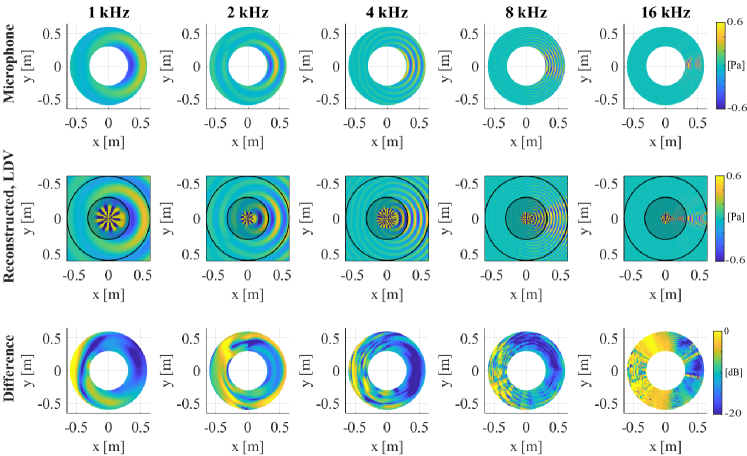
Figure 9: Experimental sound field reconstruction results from LDV projections. Sound fields are created at different frequencies from 1 kHz to 16 kHz The reference sound pressure is recorded by the microphone placed nearest the laser path.

To validate the effectiveness of the proposed method for experimental data, we generated harmonic sound fields at frequencies 1 kHz, 2 kHz, 4 kHz, 8 kHz, and 16 kHz and compared the reconstructed sound fields by CHE with the fields measured by a microphone. The results shown in Fig. 9 indicate that the proposed CHE algorithm effectively reconstructs the sound fields from LDV projections. Notably, it should be emphasized that our LDV device introduces a signal latency of 900$\,\mu$s, which necessitates compensation when comparing the reconstructed sound fields with the reference sound fields recorded by the microphone. The precision of sound field reconstruction is demonstrated by visualizing images depicting the difference between microphone and LDV reconstructions. These images are presented in the third row of Fig. 9. We estimated the difference using the same method as estimating reconstruction errors, as discussed in Section III-B. The experimental results indicate variations in the discrepancy between the reconstructed LDV sound field and the microphone signal across different frequencies. At 1 kHz, a relatively substantial difference is observed, whereas, at 16 kHz, the difference is reduced, though still present. In contrast, at 2 kHz, 4 kHz, and 8 kHz, the difference falls within the range of [-20,-10], underscoring the acceptable quality of the reconstructed sound fields. These findings reveal the persistence of minor reconstruction errors, which can be attributed to uncertainties in phase delays and amplitude losses in the signals recorded by both the microphone and LDV devices.

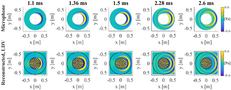
Figure 10: Time-domain sound field reconstruction.

IV-C Time-domain sound-field reconstruction

In order to assess the performance of time-domain sound field reconstruction, a 2 kHz sinusoidal burst wave with a duration of 10 ms was emitted from the loudspeaker. The experimental configuration utilized for this evaluation is consistent with the parameters defined in Section IV-A. To reconstruct the sound field in the time domain from experimentally acquired data, the procedure comprises the following steps:

• Step 1: Perform a Fast Fourier Transform (FFT) on all time-domain LDV projection data, to convert projections from the time domain to the frequency domain.

• Step 2: Apply the proposed CHE algorithm to reconstruct the sound field in the frequency domain from the FFT output data obtained in Step 1, independently for each frequency.

• Step 3: Combine the 2-dimensional (2D) reconstructed sound fields at all frequencies into a 3-dimensional (3D) array. The third dimension represents frequencies ranging from 0 Hz to the maximum frequency, with a length identical to the FFT length in Step 1.

• Step 4: Perform an inverse FFT on the 3D array of reconstructed sound fields in the frequency domain to yield the results of the time-domain sound field reconstruction.

Fig. 10 illustrates multiple frames extracted from time-domain sound fields reconstructed using LDV projections at various time points: 1.1 ms, 1.36 ms, 1.5 ms, 2.28 ms, and 2.6 ms. Concurrently, time-domain microphone signals were acquired synchronously with the LDV device for reference. To enable a meaningful comparison with the microphone signals, a delay of 900$\,\mu$s in the LDV signal was corrected. Additionally, we empirically determined the response delay of the microphone system as approximately 10$\,\mu$s through experimental measurements. Upon scrutinizing the data, it is evident that minor temporal disparities of approximately 90$\,\mu$s persist between the sound fields captured by the microphone and those recorded by the LDV device. These slight variations are attributed to undetermined signal delays within the LDV or microphone circuitry. Nevertheless, it is noteworthy that the sound fields reconstructed using the CHE algorithm from LDV projections exhibit a remarkable similarity to the corresponding microphone signals.

V Discussions

In order to expedite the process of sound field reconstruction, two key aspects are considered: reducing the number of required projections $M$ and determining an appropriate number of circular harmonics $N$.

V-A Influence of expansion order

The appropriate selection of the value $N$ is visually depicted in Fig. LABEL:fig:11a. This figure illustrates the number of circular harmonic waves required to fully represent the amplitude of the expansion coefficients, denoted as $\left|\mathbf{a}\right|$. When we examine our experimental data, we determine that the suitable $N$ values are 3, 5, 10, 20, and 30 for sound fields at 1 kHz, 2 kHz, 4 kHz, 8 kHz, and 16 kHz, respectively. This selection is based on the fact that the amplitude of expansion coefficients converges to zero when the circular harmonics index falls within the range of [-N: N]. In contrast, computational simulations suggest that the appropriate $N$ values are 7, 10, and 20 for sound fields at 1 kHz, 2 kHz, and 4 kHz, respectively. However, for sound fields at 8 kHz and 16 kHz, the amplitudes of the CHE coefficients do not converge to zero even when $N$ equals 30 (for 8 kHz) or 40 (for 16 kHz). It is worth noting that higher frequencies necessitate larger values for $N$ which in turn require more computational time for the reconstruction process. Therefore, in our simulations, we opted for $N$ values of 30 for 8 kHz, and 40 for 16 kHz, as these values adequately represent the majority of the CHE coefficient amplitudes.

Furthermore, Fig. LABEL:fig:11b elucidates the experimental sound-field reconstruction scenarios in instances where varying numbers of circular harmonic waves are employed, leading to cases of good fit, underfitting, and overfitting. A good fit is achieved when the minimum number of circular harmonics is adequate to fully represent the amplitude of the expansion coefficient. Underfitting occurs when there is a loss of amplitude due to the utilization of an insufficient number of circular harmonics. Conversely, overfitting occurs when an excessive number of circular harmonics are utilized to represent the expansion coefficient, resulting in the emergence of complex patterns extending beyond the boundaries of the sound source area. This can be observed in the overfitting cases with N = 20, and N = 25. At a frequency of 2 kHz, a good fit is achieved when the parameter falls within the range of $5\leq N\leq 15$. Underfitting occurs when $N\,<\,5$, and overfitting arises when $N>15$. To determine an appropriate value for a good model fit at frequencies other than 2 kHz, a reference can be made to Fig. LABEL:fig:11a.

V-B Influence of number of projections

In order to determine the optimal number of projections necessary for sound field reconstruction, we conducted an assessment of the reconstructed sound field quality employing NMSE analysis. A 2 kHz sound signal was emitted from a loudspeaker placed in an anechoic chamber, with the sound source positioned at an off-center location [0.12, 0]. During this analysis, we explored a range of projection quantities, ranging from 72 projections originating from the innermost concentric circle with a radius of $0.3\,$m to 2232 projections obtained from 31 concentric circles, with radii varying from $0.3\,$m to $0.6\,$m. Specifically, this encompassed 2 concentric circles with a 15 cm increment for each step, resulting in 144 projections; 4 concentric circles with an 8 cm increment for each step, yielding 288 projections; 8 concentric circles with a 4 cm increment for each step, giving rise to 576 projections; 16 concentric circles with a 2 cm increment for each step, resulting in 1152 projections; and finally, 31 concentric circles with a 1 cm increment for each step, producing a total of 2232 projections. Fig. 12a shows the NMSE values for different numbers of the concentric circles. The highest quality is for the 31 concentric circles with NMSE of -11.458 dB. Additionally, Fig. 12a illustrates that the NMSE nearly reaches convergence when the number of concentric circles is set to 16.

To minimize the number of projections employed in the reconstruction process, it is essential to identify concentric circles that yield optimal reconstruction performance among all available concentric circles. Fig. 12b demonstrates that the choice of concentric circle radius has a significant impact on reconstruction quality. Notably, utilizing 72 projections from a circle with a radius of $R\,$=$\,0.38\,$m yields superior results, with the NMSE of -9.39 dB, surpassing other radii. Fig. 12c demonstrates the reconstruction quality when considering only 144 projections from two concentric circles while the one is fixed at $R\,$=$\,0.38\,$m. It is evident that the two concentric circles with radii of $R_{1}\,$=$\,0.38\,$m and $R_{2}\,$=$\,0.6\,$m outperform the other pairs, achieving almost the same reconstruction quality as when using all 31 circles. This outcome demonstrates that by employing a combination of projections from specific concentric circles that excel in precise sound field reconstruction, it is possible to reduce the overall number of required projections. The determination of the optimal concentric circle radius and the appropriate quantity of concentric circles is beyond the scope of this paper. However, we envision that our discoveries may provide a foundational basis for future research endeavors aimed at investigating these intriguing inquiries.

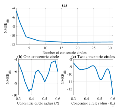
Figure 12: The assessment of the NMSE in decibels (dB) for 2 kHz reconstructed sound fields involves two scenarios: (a) the NMSE is evaluated by varying the number of projections acquired from concentric circles with radii ranging from $R_{\mathrm{min}}\,$=$\,0.3\,$m to $R_{\mathrm{max}}\,$=$\,0.6\,$m; (b) the NMSE is assessed using 72 projections from a single concentric circle; (c) NMSE evaluation when considering only 144 projections from two concentric circles $R=0.38\,$m and $R_{2}$.

VI Conclusion

This paper introduces an innovative approach involving concentric circle sampling and a two-dimensional exterior sound-field reconstruction technique based on the extension of circular harmonics. The proposed reconstruction method effectively reconstructs the sound field, particularly when the sound source is located within the reconstruction area. To evaluate the effectiveness of the proposed approach, comprehensive assessments are conducted through numerical simulations and real-world experiments. The outcomes of these simulations and experiments compellingly establish that the proposed technique outperforms conventional reconstruction methods, exhibiting superior accuracy, and concurrently minimizing the number of required measured projections for the reconstruction process. This study introduces significant advancements in acoustic data measurement and analysis, allowing for comprehensive spatiotemporal sound field capture across extensive spatial regions. Moreover, this methodology holds potential value in diverse disciplines that focus on wave field measurement and visualization.

References

- [1] A. Torras-Rosell, S. Barrera-Figueroa, and F. Jacobsen, “Sound field reconstruction using acousto-optic tomography,” The Journal of the Acoustical Society of America, vol. 131, no. 5, pp. 3786–3793, 2012.
- [2] S. A. Verburg, K. Ishikawa, E. Fernandez-Grande, and Y. Oikawa, “A century of acousto-optics- from early discoveries to modern sensing of sound with light,” Acoust. Today, vol. 19, pp. 54–62, 2023.
- [3] K. Nakamura, M. Hirayama, and S. Ueha, “Measurements of air-borne ultrasound by detecting the modulation in optical refractive index of air,” in Proc. IEEE Ultrasonics Symposium, 2002, pp. 609–612.
- [4] A. Harland, J. Petzing, and J. Tyrer, “Non-invasive measurements of underwater pressure fields using laser doppler velocimetry,” J. Sound Vib., vol. 252, pp. 169–177, 4 2002.
- [5] K. Ishikawa, K. Yatabe, N. Chitanont, Y. Ikeda, Y. Oikawa, T. Onuma, H. Niwa, and M. Yoshii, “High-speed imaging of sound using parallel phase-shifting interferometry,” Opt. Express, vol. 24, p. 12922, 6 2016.
- [6] O. Matoba, H. Inokuchi, K. Nitta, and Y. Awatsuji, “Optical voice recorder by off-axis digital holography,” Opt. Lett., vol. 39, p. 6549, 11 2014.
- [7] K. Ishikawa, R. Tanigawa, K. Yatabe, Y. Oikawa, T. Onuma, and H. Niwa, “Simultaneous imaging of flow and sound using high-speed parallel phase-shifting interferometry,” Opt. Lett., vol. 43, p. 991, 3 2018.
- [8] S. K. Rajput, O. Matoba, and Y. Awatsuji, “Holographic multi-parameter imaging of dynamic phenomena with visual and audio features,” Opt. Lett., vol. 44, p. 995, 2 2019.
- [9] Y. Takase, K. Shimizu, S. Mochida, T. Inoue, K. Nishio, S. K. Rajput, O. Matoba, P. Xia, and Y. Awatsuji, “High-speed imaging of the sound field by parallel phase-shifting digital holography,” Appl. Opt., vol. 60, p. A179, 2 2021.
- [10] S. K. Rajput, O. Matoba, M. Kumar, X. Quan, and Y. Awatsuji, “Sound wave detection by common-path digital holography,” Opt. Lasers Eng., vol. 137, p. 106331, 2 2021.
- [11] Z. Zhong, C. Wang, L. Liu, Y. Liu, L. Yu, B. Liu, and M. Shan, “Visual measurement of instable sound field using common-path off-axis digital holography,” Opt. Lasers Eng., vol. 158, p. 107129, 11 2022.
- [12] K. Ishikawa, Y. Shiraki, T. Moriya, A. Ishizawa, K. Hitachi, and K. Oguri, “Low-noise optical measurement of sound using midfringe locked interferometer with differential detection,” J. Acoust. Soc. Am., vol. 150, pp. 1514–1523, 8 2021.
- [13] B. P. Flannery, H. W. Deckman, W. G. Roberge, and K. L. D’Amico, “Three-dimensional x-ray microtomography,” Science, vol. 237, no. 4821, pp. 1439–1444, 1987.
- [14] A. C. Kak and M. Slaney, Principles of computerized tomographic imaging. SIAM, 2001.
- [15] Y. Oikawa, Y. Ikeda, M. Goto, T. Takizawa, and Y. Yamasaki, “Sound field measurements based on reconstruction from laser projections,” in Proc. (ICASSP ’05). IEEE International Conference on Acoustics, Speech, and Signal Processing, 2005., vol. 4. IEEE, pp. 661–664.
- [16] E. Koponen, J. Leskinen, T. Tarvainen, and A. Pulkkinen, “Acoustic pressure field estimation methods for synthetic schlieren tomography,” The Journal of the Acoustical Society of America, vol. 145, no. 4, pp. 2470–2479, 2019.
- [17] D. Hermawanto, K. Ishikawa, K. Yatabe, and Y. Oikawa, “Determination of frequency response of mems microphone from sound field measurements using optical phase-shifting interferometry method,” Applied Acoustics, vol. 170, p. 107523, 2020.
- [18] K. Yatabe, K. Ishikawa, and Y. Oikawa, “Acousto-optic back-projection: Physical-model-based sound field reconstruction from optical projections,” Journal of Sound and Vibration, vol. 394, pp. 171–184, 2017.
- [19] S. A. Verburg and E. Fernandez-Grande, “Acousto-optical volumetric sensing of acoustic fields,” Physical Review Applied, vol. 16, no. 4, p. 044033, 2021.
- [20] K. Ishikawa, K. Yatabe, and Y. Oikawa, “Physical-model-based reconstruction of axisymmetric three-dimensional sound field from optical interferometric measurement,” Measurement Science and Technology, vol. 32, no. 4, p. 045202, 2021.
- [21] S. A. Verburg, E. G. Williams, and E. Fernandez-Grande, “Acousto-optic holography,” J. Acoust. Soc. Am., vol. 152, pp. 3790–3799, 12 2022.
- [22] E. G. Williams and J. A. Mann III, “Fourier acoustics: sound radiation and nearfield acoustical holography,” 2000.
- [23] Y. Ren and Y. Haneda, “2D local exterior sound field reproduction using an addition theorem based on circular harmonic expansion,” in 2021 IEEE Workshop on Applications of Signal Processing to Audio and Acoustics (WASPAA). IEEE, 2021, pp. 271–275.
- [24] Y. Ren and Y. Haneda, “Two-dimensional exterior sound field reproduction using two rigid circular loudspeaker arrays,” The Journal of the Acoustical Society of America, vol. 148, no. 4, pp. 2236–2247, 2020.