On the Convergence of Encoder-only
Shallow Transformers

Abstract

In this paper, we aim to build the global convergence theory of encoder-only shallow Transformers under a realistic setting from the perspective of architectures, initialization, and scaling under a finite width regime. The difficulty lies in how to tackle the softmax in self-attention mechanism, the core ingredient of Transformer. In particular, we diagnose the scaling scheme, carefully tackle the input/output of softmax, and prove that quadratic overparameterization is sufficient for global convergence of our shallow Transformers under commonly-used He/LeCun initialization in practice. Besides, neural tangent kernel (NTK) based analysis is also given, which facilitates a comprehensive comparison. Our theory demonstrates the separation on the importance of different scaling schemes and initialization. We believe our results can pave the way for a better understanding of modern Transformers, particularly on training dynamics.

1 Introduction

Transformers (Vaswani et al., 2017) have demonstrated unparalleled success in influential applications (Devlin et al., 2019; Brown et al., 2020; Wang et al., 2018; Dosovitskiy et al., 2021; Liu et al., 2022b). A fundamental theoretical topic concerns the global convergence, i.e., the training dynamics of Transformers, which would be helpful for further analysis, e.g., in-context learning (von Oswald et al., 2022; Akyürek et al., 2023), generalization (Li et al., 2023). In fact, even within a simplified Transformer framework under certain specific regimes, the global convergence guarantees still remain an elusive challenge.

To theoretically understand this, let us first recall the exact format of the self-attention mechanism, the core ingredient of the Transformer. Given the input ${\bm{X}}\in\mathbb{R}^{d_{s}\times d}$ ($d_{s}$ is the number of tokens and $d$ is the feature dimension of each token), a self-attention mechanism is defined as:

$$\text{Self-attention}(\bm{X})\triangleq\sigma_{s}\left(\tau_{0}({\bm{X}}{{\bm{W}}}_{Q}^{\top})\left({\bm{X}}{\bm{W}}_{K}^{\top}\right)^{\top}\right)\left({\bm{X}}{\bm{W}}_{V}^{\top}\right)=\sigma_{s}\left({\color[rgb]{0,0,1}\tau_{0}}{\bm{X}}{\color[rgb]{0,0,1}{{\bm{W}}}_{Q}^{\top}{\bm{W}}_{K}}{\bm{X}}^{\!\top}\right)\left({\bm{X}}{\bm{W}}_{V}^{\top}\right)\,,$$

where $\sigma_{s}$ is the row-wise softmax function, $\tau_{0}\in\mathbb{R}^{+}$ is the scaling factor, and the learnable weights are ${{\bm{W}}}_{Q},{{\bm{W}}}_{K},{{\bm{W}}}_{V}\in\mathbb{R}^{d_{m}\times d}$ with the width $d_{m}$. Given $\bm{X}$, the input of softmax depends on $\tau_{0}\bm{W}^{\!\top}_{Q}\bm{W}_{K}$, including the scaling factor $\tau_{0}$ and initialization schemes for learnable parameters, and thus determines the output of softmax and then affects the performance of Transformers in both theory and practice. There are several scaling schemes in previous literature. For instance, given $\bm{W}_{Q}$ and $\bm{W}_{K}$ initialized by standard Gaussian, the scaling factor $\tau_{0}$ is chosen by

• $\tau_{0}=d_{m}^{-1/2}$ in the original Transformer (Vaswani et al., 2017): each element in $\tau_{0}\bm{W}^{\!\top}_{Q}\bm{W}_{K}$ is a random variable with mean $0$ and variance $1$. This scaling avoids the blow-up of value inside softmax as $d_{m}$ increases  (Hron et al., 2020).

• $\tau_{0}=d_{m}^{-1}$: This scaling stems from the neural tangent kernel (NTK) analysis (Jacot et al., 2018), a commonly used technical tool for convergence analysis of fully-connected (or convolutional) networks under an infinite-width setting $d_{m}\to\infty$. However, for Transformer, if one uses this scaling under the infinite-width setting, then by the law of large numbers, we have $\lim_{d_{m}\to\infty}\tau_{0}[\bm{W}^{\!\top}_{Q}\bm{W}_{K}]^{(ij)}=0$. As a result, the input of softmax is zero and the softmax degenerates to a pooling layer. That means, the non-linearity is missing, which motivates researchers to carefully rethink this setting.

For instance, under the $\tau_{0}=d_{m}^{-1}$ setting, Yang (2020) use the same query and key matrices to prevent the softmax from degenerating into a pooling layer. Besides, to avoid the analytic difficulty of softmax due to the fact that each element of the output depends on all inputs,  Hron et al. (2020) substitute softmax with ReLU under the $\tau_{0}=d_{m}^{-1/2}$ and infinite width setting for simplicity.

Clearly, there exists a gap between theoretical analysis and practical architectures on the use of softmax, and accordingly, this leads to the following open question:

How can we ensure the global convergence of Transformers under a realistic setting?

The primary contribution of this work is to establish the convergence theory of shallow Transformer under a realistic setting. Despite its shallow and encoder-only architecture, our Transformer model captures all the fundamental components found on typical Transformers, including the self-attention mechanism with the softmax activation function, one feedforward ReLU layer, one average pooling layer, and a linear output layer, cf. Eq. .2. We adopt the $\tau_{0}=d_{m}^{-1/2}$ scaling under the finite-width setting and compare the results of LeCun/He initializations, which are commonly used in practical applications. Besides, the convergence result under the $\tau_{0}=d_{m}^{-1}$ setting (as well as the NTK-based analysis) is also studied, which facilitates a comprehensive comparison. Our theoretical results demonstrate notable separations among scaling settings, initializations, and architectures as below:

• Scaling: The global convergence can be achieved under both $\tau_{0}=d_{m}^{-1/2}$ and $\tau_{0}=d_{m}^{-1}$. Nevertheless, as suggested by our theory: for a small $d_{m}$, there is no significant difference for these two scaling schemes on the convergence; but for a large enough $d_{m}$, the $\tau_{0}=d_{m}^{-1/2}$ scaling admits a faster convergence rate of Transformers than that with $\tau_{0}=d_{m}^{-1}$. Interestingly, under this $\tau_{0}=d_{m}^{-1}$ setting, our theory also demonstrates the separation on the convergence result, depending on whether the input is formed along sequence dimension ($d=1$) or embedding dimension ($d_{s}=1$).

• Initialization: Under LeCun and He initialization, our shallow Transformer admits a faster convergence rate than the NTK initialization. This could be an explanation for the seldom usage of NTK initialization for Transformer training in practice.

• Architecture: Quadratic over-parameterization is enough to ensure the global convergence of our shallow Transformer. As a comparison, if the self-attention mechanism is substituted by a feed-forward ReLU layer, our shallow Transformer is close to a three-layer fully-connected ReLU neural networks to some extent, requiring cubic over-parameterization for global convergence.

We firmly believe that our theoretical analysis takes a significant step towards unraveling the mysteries behind Transformers from the perspective of global convergence. We hope that our analytical framework and insights on various initialization and scaling techniques would be helpful in training modern, large-scale Transformer-based models (Radford et al., 2018; Brown et al., 2020).

2 Related work

Self-attention, Transformer: Regarding training dynamics, Snell et al. (2021) explains why single-head attention focuses on salient words by analyzing the evolution throughout training. Hron et al. (2020) show that the output of Transformer converges to Gaussian process kernel and provide the NTK formulation of Transformer. Recently, Li et al. (2023) provide sample complexity of shallow Transformer to study its generalization property under a good initialization from pretrained model. The separation between the Transformer and CNN is recently explored. Jelassi et al. (2022) provably demonstrate that Vision Transformer (ViT) has the ability to learn spatial structure without additional inductive bias such as the spatial locality in CNN. Chen et al. (2022) study the loss landscape of ViT and find that ViT converges at sharper local minima than ResNet. Park and Kim (2022) show that ViT is a low-pass filter while CNN is a high-pass filter, thus, these two models can be complementary.

NTK, lazy training, Hessian: The NTK was introduced by Jacot et al. (2018) to connect the infinite-width neural network trained by gradient descent and the kernel regression. The roles of such kernel include analysis of the training dynamics of the neural network in the over-parameterization regime (Allen-Zhu et al., 2019a; Chizat et al., 2019; Du et al., 2019a, b; Zou et al., 2020). The global convergence, generalization bound, and memorization capacity largely depend on the minimum eigenvalue of the NTK (Cao and Gu, 2019; Zhu et al., 2022; Nguyen et al., 2021; Bombari et al., 2022). Even though the NTK is extended from FCNN to several typical networks including Transformer (Tirer et al., 2020; Huang et al., 2020; Arora et al., 2019b; Alemohammad et al., 2021; Nguyen and Mondelli, 2020), it has not been used to analyze the global convergence of Transformer. On the other hand, the stability of the tangent kernel during training is required when connecting to kernel regression, but such stability can not be explained by the phenomenon of lazy training (Chizat et al., 2019), which indicates a small change of the parameters from initialization. The hessian spectral bound is the main reason for the stability of kernel, as mentioned in Liu et al. (2020).

Over-parameterization for convergence analysis: Due to over-parameterization, neural networks (NNs) can fit arbitrary labels with zero training loss when trained with (stochastic) gradient descent (SGD), both theoretically Li and Liang (2018); Du et al. (2019b) and empirically (Zhang et al., 2017). This leads to an interesting question in theory: how much overparameterization is enough to ensure global convergence of NNs? A common recipe for the proof of global convergence relies on the variant of Polyak-Lojasiewicz condition (Polyak, 1963; Liu et al., 2022a), NTK (Du et al., 2019b, a; Zou and Gu, 2019; Allen-Zhu et al., 2019a), or the minimum eigenvalue of the gram matrix (Nguyen, 2021; Bombari et al., 2022). In Section B.3, we provide a comprehensive overview of a recent line of work that improves the over-parameterization condition for ensuring the convergence of NNs. However, the over-parameterization condition for Transformer to achieve global convergence remains elusive from existing literature and we make an initial step towards this question.

3 Problem setting

This section includes the problem setting with notations and model formulation of the shallow Transformer that is studied in this paper.

3.1 Notation

Vectors (matrices) are symbolized by lowercase (uppercase) boldface letters, e.g., ${\bm{w}}$, ${\bm{W}}$. We use $\|\cdot\|_{\mathrm{F}}$ and $\|\cdot\|_{2}$ to represent the Frobenius norm and the spectral norm of a matrix, respectively. The Euclidean norm of a vector is symbolized by $\|\cdot\|_{2}$. The superscript with brackets is used to represent the element of a vector/matrix, e.g., $w^{(i)}$ is the $i^{\text{th}}$ element of ${\bm{w}}$. The superscript without brackets symbolizes the parameters at different training step, e.g., ${\bm{\theta}}^{t}$. We denote by $[N]=\{1,\dots,N\}$ for short. We use $\sigma_{\min}(\cdot)$ and $\lambda_{\min}(\cdot)$ to represent the minimum singular value and minimum eigenvalue of a matrix. The NTK matrix and hessian matrix of the network are denoted by ${\bm{K}}$ and ${\bm{H}}$, respectively. The order notation, e.g., $\widetilde{\mathcal{O}}$, $\widetilde{\Omega}$, omits the logarithmic factor. More detailed notation can be found in Table 2 of the appendix.

Let $X\subseteq\mathbb{R}^{d_{s}\times d}$ be a compact metric space with $d_{s}\leq d$ and $Y\subseteq\mathbb{R}$, where $d$ is the dimension of each token, $d_{s}$ is the total sequence length of the input. The training set $\{({\bm{X}}_{n},y_{n})\}_{n=1}^{N}$ is assumed to be iid sampled from an unknown probability measure on $X\times Y$. In this paper, we focus the regression task by employing the squared loss. The goal of our regression task is to find a hypothesis, i.e., a Transformer $f:X\rightarrow Y$ in our work, such that $f({\bm{X}};{\bm{\theta}})$ parameterized by ${\bm{\theta}}$ is a good approximation of the label $y\in Y$ corresponding to a new sample ${\bm{X}}\in X$. We use a vector ${\bm{\theta}}$ to denote the collection of all learnable parameters.

3.2 Model formulation of shallow Transformer

Throughout this work, we consider the encoder of Transformer, which can be applied to both regression and classification tasks (Yüksel et al., 2019; Dosovitskiy et al., 2021). Given an input ${\bm{X}}\in\mathbb{R}^{d_{s}\times d}$, the model is defined as below:

$${\bm{A}}_{1}=\text{Self-attention}(\bm{X})\triangleq\sigma_{s}\left(\tau_{0}({\bm{X}}{{\bm{W}}}_{Q}^{\top})\left({\bm{X}}{\bm{W}}_{K}^{\top}\right)^{\top}\right)\left({\bm{X}}{\bm{W}}_{V}^{\top}\right),$$ (.1)

$${\bm{A}}_{2}=\tau_{1}\sigma_{r}{({\bm{A}}_{1}{\bm{W}}_{H})}\,,\qquad{\bm{a}}_{3}=\varphi{({\bm{A}}_{2})},\qquad f({\bm{X}};{\bm{\theta}})={\bm{a}}_{3}^{\top}{\bm{w}}_{O}\,,$$ (.2)

where the output is $f({\bm{X}};{\bm{\theta}})\in\mathbb{R}$, $\tau_{0}$ and $\tau_{1}$ are two scaling factors.

The ingredients of a Transformer with width $d_{m}$ are defined as follows:

• A self-attention mechanism (Eq. .1): $\sigma_{s}$ is the row-wise softmax function; the learnable parameters are ${{\bm{W}}}_{Q},{{\bm{W}}}_{K},{{\bm{W}}}_{V}\in\mathbb{R}^{d_{m}\times d}$. We employ Gaussian initialization ${{\bm{W}}}_{Q}^{(ij)}\sim\mathcal{N}(0,\eta_{Q})$, ${{\bm{W}}}_{K}^{(ij)}\sim\mathcal{N}(0,\eta_{K})$, ${{\bm{W}}}_{V}^{(ij)}\sim\mathcal{N}(0,\eta_{V})$ with $i\in[d_{m}]$ and $j\in[d]$. Refer to Section 3.2 for typical initialization examples.

• A feed-forward ReLU layer (in Eq. .2): $\sigma_{r}$ is the ReLU activation function; the learnable parameter is ${\bm{W}}_{H}\in\mathbb{R}^{d_{m}\times d_{m}}$. Following Yang et al. (2022), we combine ${\bm{W}}_{V}$ and ${\bm{W}}_{H}$ together (by setting ${\bm{W}}_{H}={\bm{I}}$ ) for ease of the analysis. Note that it does not mean its training dynamics are the same as the joint-training of these two adjacent matrices.

• An average pooling layer (in Eq. .2): $\varphi$ indicates the column-wise average pooling. Note that the average pooling layer is applied along the sequence length dimension to ensure the final output is a scalar, which is commonly used in practical Vision Transformer or theoretical analysis (Dosovitskiy et al., 2021; Yang, 2020).

• An output layer (in Eq. .2) with learnable parameter ${\bm{w}}_{O}\in\mathbb{R}^{d_{m}}$, initialized by ${\bm{w}}_{O}^{(i)}\sim\mathcal{N}(0,\eta_{O})$.

Remarks: Proper initialization and scaling are required to ensure the convergence and learnability, as seen in previous work (Jacot et al., 2018; Tirer et al., 2022; Lee et al., 2019). For our convergence analysis, we consider standard Gaussian initialization with different variances and different scaling factor that includes three typical initialization schemes in practice. In Section 3.2, we detail the formula of LeCun initialization, He initialization, and NTK initialization.

Given $N$ input samples $\{{{\bm{X}}_{n}}\}_{n=1}^{N}$, the corresponding ground truth label, the final output of network, and the output of the last hidden layer, are denoted by:

$${\bm{y}}\triangleq\{y_{n}\}_{n=1}^{N}\in\mathbb{R}^{N},\quad{\bm{f}}({\bm{\theta}})\triangleq\{f({\bm{X}}_{n};{\bm{\theta}})\}_{n=1}^{N}\in\mathbb{R}^{N},\quad{\bm{F}}_{\mathrm{pre}}({\bm{\theta}})\triangleq\{{\bm{a}}_{3}({\bm{X}}_{n};{\bm{\theta}})\}_{n=1}^{N}\in\mathbb{R}^{N\times d_{m}}.$$

We consider standard gradient descent (GD) training of Transformer, as illustrated in Algorithm 1. Here the squared loss is expressed as $\ell({\bm{\theta}})=\frac{1}{2}\left\lVert{\bm{f}}({\bm{\theta}})-{\bm{y}}\right\rVert_{2}^{2}$.

Table 1: Common initialization methods with their variances of Gaussian distribution and scaling factors. The choice of $\tau_{1}=d_{m}^{-1/2}$ is based on standard NTK initialization on prior literature (Du et al., 2019b).

Init.	$\eta_{O}$	$\eta_{V}$	$\eta_{Q}$	$\eta_{K}$	$\tau_{1}$
LeCun	$d_{m}^{-1}$	$d^{-1}$	$d^{-1}$	$d^{-1}$	$1$
He	$2d_{m}^{-1}$	$2d^{-1}$	$2d^{-1}$	$2d^{-1}$	$1$
NTK	1	1	1	1	$d_{m}^{-1/2}$

  Input: data $({\bm{X}}_{n},y_{n})_{n=1}^{N}$, step size $\gamma$.

  Initialize weights as follows:

$\quad\,\,{\bm{\theta}}^{0}:=\{{{\bm{W}}}_{Q}^{0},{{\bm{W}}}_{K}^{0},{{\bm{W}}}_{V}^{0},{{\bm{W}}}_{O}^{0}\}.$

  for $t=0$ to $t^{\prime}-1$ do

      ${\bm{W}}_{Q}^{t+1}={{\bm{W}}}_{Q}^{t}-\gamma\cdot\nabla_{{{\bm{W}}}_{Q}}\ell({\bm{\theta}}^{t})$, ${{\bm{W}}}_{K}^{t+1}={{\bm{W}}}_{K}^{t}-\gamma\cdot\nabla_{{{\bm{W}}}_{K}}\ell({\bm{\theta}}^{t})$,

${{\bm{W}}}_{V}^{t+1}={{\bm{W}}}_{V}^{t}-\gamma\cdot\nabla_{{{\bm{W}}}_{V}}\ell({\bm{\theta}}^{t})$, ${{\bm{W}}}_{O}^{t+1}={{\bm{W}}}_{O}^{t}-\gamma\cdot\nabla_{{{\bm{W}}}_{O}}\ell({\bm{\theta}}^{t})$.

  end for

Output: the model based on ${{\bm{\theta}}}^{t^{\prime}}$.

Algorithm 1 Gradient descent training

4 Main results

In this section, we study the convergence guarantee of Transformer training by GD under the squared loss. Firstly, we provide a general analytical framework in Section 4.1 covering different initialization schemes, where we identify the condition for achieving global convergence. Next, we validate these conditions for several practical initialization schemes under $\tau_{0}=d_{m}^{-1/2}$ in Section 4.2 and $\tau_{0}=d_{m}^{-1}$ in Section 4.3, respectively. We include NTK-based results for self-completeness. Discussion on the convergence results with different scalings, initializations, and architectures is present in Section 4.4.

4.1 General framework for convergence analysis

Before presenting our result, we introduce a basic assumption.

Assumption 1.

The input data is bounded $\|{\bm{X}}\|_{\mathrm{F}}\leq\sqrt{d_{s}}C_{x}$ with some positive constant $C_{x}$.

Remark: This assumption is standard as we can always scale the input. The embedding of token is usually assumed to have a unit norm (Li et al., 2023), which is unrelated to $d$.

Now we are ready to present our proposition, with the proof deferred to Section C.2. Notice that our proposition holds with high probability under some conditions, which depend on certain initialization schemes and scaling factors. Since our proposition is devoted to a unifying analysis framework under various initialization schemes, we do not include specific probabilities here. The validation of the required conditions and probability is deferred to Sections 4.2 and 4.3, respectively.

Proposition 1.

Consider the Transformer with $d_{m}\geq N$. Let $C_{Q},C_{K},C_{V},C_{O}$ be some positive constants, and define the following quantities at initialization for simplification:

• The norm of the parameters:

  $$\bar{\lambda}_{Q}\triangleq\left\lVert{\bm{W}}_{Q}^{0}\right\rVert_{2}+C_{Q},\;\bar{\lambda}_{K}\triangleq\left\lVert{\bm{W}}_{K}^{0}\right\rVert_{2}+C_{K},\;\bar{\lambda}_{V}\triangleq\left\lVert{\bm{W}}_{V}^{0}\right\rVert_{2}+C_{V},\;\bar{\lambda}_{O}\triangleq\left\lVert{\bm{w}}_{O}^{0}\right\rVert_{2}+C_{O}.$$

• Two auxiliary terms: $\rho\triangleq N^{1/2}d_{s}^{3/2}\tau_{1}C_{x},\quad$ $z\triangleq\bar{\lambda}_{O}^{2}\left(1+4\tau_{0}^{2}C_{x}^{4}d_{s}^{2}\bar{\lambda}_{V}^{2}\left(\bar{\lambda}_{Q}^{2}+\bar{\lambda}_{K}^{2}\right)\right)\,$.

Under Assumption 1, we additionally assume that the minimum singular value of ${\bm{F}}_{\mathrm{pre}}^{0}$, i.e., $\alpha\triangleq\sigma_{\rm min}\left({\bm{F}}_{\mathrm{pre}}^{0}\right)$ satisfies the following condition at initialization:

$$\alpha^{2}\geq 8\rho\max\left(\bar{\lambda}_{V}C_{O}^{-1},\bar{\lambda}_{O}C_{V}^{-1},2\tau_{0}C_{x}^{2}d_{s}\bar{\lambda}_{K}\bar{\lambda}_{V}\bar{\lambda}_{O}C_{Q}^{-1},2\tau_{0}C_{x}^{2}d_{s}\bar{\lambda}_{Q}\bar{\lambda}_{V}\bar{\lambda}_{O}C_{K}^{-1}\right)\sqrt{2\ell({\bm{\theta}}^{0})}\,,$$ (2)

$$\alpha^{3}\geq 32\rho^{2}z\sqrt{2\ell({\bm{\theta}}^{0})}/\bar{\lambda}_{O}\,.$$ (3)

If the step size satisfies $\gamma\leq 1/C$ with a constant $C$ depending on ($\bar{\lambda}_{Q},\bar{\lambda}_{K},\bar{\lambda}_{V},\bar{\lambda}_{O},\ell({\bm{\theta}}^{0}),\rho,\tau_{0}$), then GD converges to a global minimum as follows:

$$\ell({\bm{\theta}}^{t})\leq\left(1-\gamma\frac{\alpha^{2}}{2}\right)^{t}\ \ell({\bm{\theta}}^{0})\,,\quad\forall t\geq 0\,.$$ (4)

Remark: The parameter $\alpha$ in Eqs. 2 and 3 controls the convergence rate of global convergence, and the condition will be verified in the next subsection. The step-size $\gamma$ is inversely proportional to $N^{1/2}$ due to the construction of $C$ in Section C.2.

Proof sketch: The main idea of our convergence analysis is based on the variant of Polyak-Lojasiewicz (PL) inequality (Polyak, 1963; Nguyen, 2021), i.e., $||\nabla\ell({{\bm{\theta}}})||_{2}^{2}\geq 2\lambda_{\min}({{\bm{K}}})\ell({{\bm{\theta}}})\geq 2\lambda_{\min}({{\bm{F}}}_{\mathrm{pre}}{{\bm{F}}}_{\mathrm{pre}}^{\top})\ell({{\bm{\theta}}})$. Thus, if the minimum singular value of ${\bm{F}}_{\mathrm{pre}}$ is strictly greater than 0, then minimizing the gradient on the LHS will drive the loss to zero. To this end, Proposition. 1 can be split into two parts. First, by induction, at every time step, each parameter in the Transformer can be bounded w.h.p; the minimum singular value of ${\bm{F}}_{\mathrm{pre}}$ is bounded away for some positive quality at the initialization point. Secondly, we prove that the Lipschitzness of the network gradient, which means the loss function is almost smooth. Combining the above two results, the global convergence can be achieved. Furthermore, based on different initialization and scaling schemes, we are able to validate Eqs. 2 and 3 via the spectral norm estimation of $\bar{\lambda}_{Q}$, $\bar{\lambda}_{K}$, $\bar{\lambda}_{V}$, $\bar{\lambda}_{O}$ and a positive lower bound for ${\bm{F}}_{\mathrm{pre}}$ in the following section.

4.2 LeCun and He initialization under the $d_{m}^{-1/2}$ setting

Here we aim to show that, under the LeCun/He initialization with the setting of $d_{m}^{-1/2}$, the conditions in Eqs. 2 and 3 will be satisfied with high probability and scaling schemes in Section 3.2 and hence lead to global convergence. To derive our result, we need the following assumptions on the input data regarding the rank and dissimilarity of data.

Assumption 2.

We assume that the input data ${\bm{X}}$ has full row rank.

Remark: This assumption requires that each row $\bm{X}^{(i,:)}$ is linearly independent for any $i\in[d_{s}]$, which is fair and attainable in practice. For example, for language tasks, even though there might be some repeated token in ${\bm{X}}$, each row in ${\bm{X}}$ can be uncorrelated when added with positional embedding. Similarly, in image tasks with Visual Transformer, the raw image is grouped by patch and mapped via a linear layer to construct ${\bm{X}}$, thus each row in ${\bm{X}}$ can be uncorrelated.

Assumption 3.

For any data pair $({\bm{X}}_{n},{\bm{X}}_{n^{\prime}})$, with $n\neq n^{\prime}$ and $n,n^{\prime}\in[N]$, then we assume that $\mathbb{P}\left(\left|\left\langle{\bm{X}}_{n}^{\top}{\bm{X}}_{n},{\bm{X}}_{n^{\prime}}^{\top}{\bm{X}}_{n^{\prime}}\right\rangle\right|\geq t\right)\leq\exp(-t^{\hat{c}})$ with some constant $\hat{c}>0$.

Remark: We discuss the rationale behind this assumption:

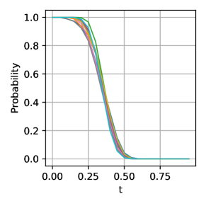
Figure 1: Validation of Asm. 3.

The idea behind Assumption 3 is that different data points admit a small similarity. To be specific, for two data points $\bm{X}_{n}$ and $\bm{X}_{n^{\prime}}$ with $n\neq n^{\prime}$, their inner product reflects the similarity of their respective (empirical) covariance matrix. We expect that this similarity is small with a high probability. The spirit of this assumption also exists in previous literature, e.g., Nguyen et al. (2021). The constant $\hat{c}$ determines the decay of data dissimilarity. A larger $\hat{c}$ results in less separable data. Our assumption has no requirement on $\hat{c}$ such that $\hat{c}$ can be small enough, which allows for a general data distribution.

Verification of assumption. Here we experimentally validate this assumption under a standard language IMDB dataset (Maas et al., 2011). We randomly sample 100 (normalized) sentences with embedding and plot the probability (frequency) of $\mathbb{P}\left(\left|\left\langle{\bm{X}}_{n}^{\top}{\bm{X}}_{n},{\bm{X}}_{n^{\prime}}^{\top}{\bm{X}}_{n^{\prime}}\right\rangle\right|\geq t\right)$ as $t$ increases. We repeat it over 10 runs and plot the result in Figure 1. We can observe an exponential decay as $t$ increases, which implies that our assumption is fair. Besides, the validation of Assumption 3 on image data, e.g., MNIST by ViT, is deferred to Section E.2.

Now we are ready to present our main theorem under the $d_{m}^{-1/2}$ setting. The proof is deferred to Section C.3.

Theorem 1.

Under the setting of LeCun/He initialization in Section 3.2 and  Assumptions 1, 2 and 3, suppose $d_{m}\geq d$, and given $\tau_{0}=d_{m}^{-1/2}$, $d_{m}=\tilde{\Omega}(N^{3})$, then with probability at least $1-8e^{-d_{m}/2}-\delta-\exp{(-\Omega((N-1)^{-\hat{c}}d_{s}^{-1}))}$ for proper $\delta$, the GD training of Transformer converges to a global minimum with sufficiently small step size $\gamma$ as in Eq. 4.

Remark: The probability relates to several randomness sources, e.g., data sampling, dissimilarity of data, and parameter initialization. The quantity $\exp{(-\Omega((N-1)^{-\hat{c}}d_{s}^{-1}))}$ can be small for a small enough $\hat{c}$ as discussed in Assumption 3. Further discussion on our result refers to Section 4.4 for details. Besides, our proof framework is also valid for the $\tau_{0}=d_{m}^{-1}$ setting. We demonstrate that $d_{m}=\tilde{\Omega}(N^{2})$ suffices to achieve global convergence, see Section C.3 for details.

Proof sketch: To check whether the conditions in Eqs. 2 and 3 hold, the key idea is to provide the lower bound of $\alpha$. Then we upper bound $\bar{\lambda}_{Q},\bar{\lambda}_{K},\bar{\lambda}_{V},\bar{\lambda}_{O}$ based on concentration inequalities to upper bound the initial loss, one key step is to utilize Gershgorin circle theorem (Gershgorin, 1931) to provide a lower bound for $\alpha$. Lastly, we plug these bound into the condition Eqs. 2 and 3 in order to obtain the requirement for the width $d_{m}$.

4.3 NTK initialization under the $d_{m}^{-1}$ setting

The NTK theory, as a representative application of the $\tau_{0}=d_{m}^{-1}$ setting, can be also used for analysis of training dynamics. We also include the NTK results in this section for self-completeness. In this section, we first derive the limiting NTK formulation of Transformer under the $d_{m}^{-1}$ scaling scheme, and then show the global convergence of Transformers.

Lemma 1.

Denote $\bm{\Phi}^{\star}=:[\frac{1}{d_{s}}{\bm{X}}_{1}^{\top}\bm{1}_{d_{s}},...,\frac{1}{d_{s}}{\bm{X}}_{N}^{\top}\bm{1}_{d_{s}}]^{\top}\in\mathbb{R}^{N\times d}$, then the limiting NTK matrix ${\bm{K}}\in\mathbb{R}^{N\times N}$ of Transformer under the NTK initialization with $\tau_{0}=d_{m}^{-1}$ has the following form:

$$\begin{split}&{\bm{K}}=d_{s}^{2}\mathbb{E}_{{\bm{w}}\sim\mathcal{N}(\bm{0},\bm{I})}\left(\sigma_{r}\left(\bm{\Phi}^{\star}{\bm{w}}\right)\sigma_{r}\left(\bm{\Phi}^{\star}{\bm{w}}\right)^{\top}\right)+d_{s}^{2}\mathbb{E}_{{\bm{w}}\sim\mathcal{N}(\bm{0},\bm{I})}\left(\dot{\sigma_{r}}\left(\bm{\Phi^{\star}}{\bm{w}}\right)\dot{\sigma_{r}}\left(\bm{\Phi}^{\star}{\bm{w}}\right)^{\top}\right)\left(\bm{\Phi}^{\star}\bm{\Phi}^{\star\top}\right).\end{split}$$

Remark: The formulation of $\bm{\Phi}^{\star}$ implies that the self-attention layer degenerates as $\frac{1}{d_{s}}\bm{1}_{d_{s}\times d_{s}}{\bm{X}}{\bm{W}}_{V}^{\top}$, i.e., the dimension missing effect as mentioned before.

Now we are ready to present our convergence result under the $d_{m}^{-1}$ scaling with the proof deferred to Section C.4.

Theorem 2.

Under the setting of NTK initialization in Section 3.2 and Assumptions 1, 2 and 3 , suppose $d_{m}=\tilde{\Omega}(N)$, then with probability at least $1-8e^{-d_{m}/2}-\delta-\exp{(-\Omega((N-1)^{-\hat{c}}d_{s}^{-1}))}$, the GD training of Transformer converges to a global minimum with sufficiently small $\gamma$ as in Eq. 4.

Proof sketch: The overall idea is the same as the proof of the previous theorem, i.e., we need to provide the lower bound of $\alpha$. However, in this case, the limit for the output of softmax exists so that we can apply concentration inequality to lower bound the $\alpha$. Lastly, we plug these bound into the condition Eqs. 2 and 3 in order to obtain the requirement for the width $d_{m}$. Besides, the stability of NTK during training allows us to build a connection on training dynamics between the Transformer (assuming a squared loss) and the kernel regression predictor. Next, in order to show that the NTK is stable during GD training, below we prove that the spectral norm of Hessian is controlled by the width.

Theorem 3 (Hessian norm is controlled by the width).

Under Assumption 1 and scaling $\tau_{0}=d_{m}^{-1}$, given any fixed $R>0$, and any ${\bm{\theta}}^{t}\in B({\bm{\theta}},R):=\{{\bm{\theta}}:\|{\bm{\theta}}-{\bm{\theta}}^{0}\|_{2}\leq R\}$, ${\bm{\theta}}^{0}$ as the weight at initialization, then with probability at least $1-8e^{-d_{m}/2}$, the Hessian spectral norm of Transformer satisfies: $\|{\bm{H}}({\bm{\theta}}^{t})\|_{2}\leq\mathcal{O}{\left(d_{m}^{-1/2}\right)}$.

Remark: By (Liu et al., 2020, Proposition 2.3), the small Hessian norm is a sufficient condition for small change of NTK. Thus, Theorem 3 can be an indicator for the stability of NTK. Besides, Theorem 3 supplements the result in (Park and Kim, 2022) which exhibits empirically a relationship between the Hessian norm and the width but lacks theoretical proof.

4.4 Discussion on convergence results

We compare the derived results under different scaling schemes, initializations, and architectures.

Comparison of scaling schemes: The global convergence can be achieved under both $\tau_{0}=d_{m}^{-1/2}$ and $\tau_{0}=d_{m}^{-1}$. Nevertheless, as suggested by our theory, for a small $d_{m}$, there is no significant difference between these two scaling schemes on the convergence; but for a large enough $d_{m}$, the $\tau_{0}=d_{m}^{-1/2}$ scaling admits a faster convergence rate of Transformers than that of $\tau_{0}=d_{m}^{-1}$ due to a more tight estimation of the lower bound of $\alpha$, see Section C.6 for details. The intuition behind the lower convergence rate under the setting of large width and $\tau_{0}=d_{m}^{-1}$ is that the input of softmax is close to zero such that softmax roughly degenerates as a pooling layer, losing the ability to fit data. This can be also explained by Lemma 1 from the perspective of dimension missing: self-attention (${\bm{X}}$) degenerates as $\frac{1}{d_{s}}\bm{1}_{d_{s}\times d_{s}}{\bm{X}}{\bm{W}}_{V}^{\top}$.

The result under the $\tau_{0}=d_{m}^{-1}$ setting requires weaker over-parameterization than the $\tau_{0}=d_{m}^{-1/2}$ setting. Nevertheless, we do not claim that $\tau_{0}=d_{m}^{-1}$ is better than $\tau_{0}=d_{m}^{-1/2}$. This is because, under the over-parameterization regime, the scaling $\tau_{0}=d_{m}^{-1}$ makes the self-attention layer close to a pooling layer. This analysis loses the ability to capture the key characteristics of the self-attention mechanism in Transformers.

Note that the lower bound of the minimum eigenvalue is in the constant order, which is tight (since it matches the upper bound). Based on this, by studying the relationship between $d_{m}$ and $\lambda_{0}$, we can prove that quadratic (cubic) over-parameterization is required for $d_{m}^{-1}$ ($d_{m}^{-1/2}$) scaling. This quadratic over-parameterization requirement could be relaxed if a better relationship is given while it is still unclear and beyond our proof technique.

Comparison on initializations: Though our results achieve the same convergence rate under these initialization schemes, we can still show the separation on $\alpha$ that affects the convergence in Eq. 4 among these initialization schemes. To be specific, we verify that under LeCun and He initialization, the lower bound of $\alpha^{2}$ is tighter than that of NTK initialization, and hence admits faster convergence, see Section C.5 for further details. This can be an explanation of the seldom usage of NTK initialization in practice. Besides, the NTK initialization scheme allows for a larger step size than LeCun/He initialization for training. That means, if $\alpha$ is the same in these three initialization schemes, we usually choose a large step size under the NTK initialization scheme, see Section E.1.

Comparison on architectures: Note that the Transformer defined in Eq. .2 includes a self-attention layer, a feedforward ReLU layer, and an output layer. Our result proves that a cubic (quadratic) over-parameterization condition is required for $d_{m}^{-1/2}$ ($d_{m}^{-1}$) under LeCun initialization. As a comparison, a three-layer fully-connected ReLU network under LeCun initialization requires $d_{m}=\tilde{\Omega}(N^{3})$ (Nguyen, 2021).

The aforementioned result holds for matrix input. Although not as frequent, some data inputs are naturally in vector form. Two ways to feed the input into Transformer are either formulating along sequence dimension ($d=1$) or along embedding dimension ($d_{s}=1$). The following result shows the separation under these two settings to understand when the Transformer works well or not regarding the input.

Corollary 1 (Convergence of vector input).

Consider LeCun initialization with $\tau_{0}=d_{m}^{-1}$ scaling, given vector input ${\bm{x}}\in\mathbb{R}^{\tilde{d}}$, if one feeds the input to Transformer by setting $d_{s}=1,d=\tilde{d}$, then training with GD can converge to a global minimum. On the contrary, if one sets $d_{s}=\tilde{d},d=1$, the conditions in Eqs. 2 and 3 do not hold, the convergence can not be guaranteed by our theory.

Remark: Such a result is motivated by considering least squares. Specifically, given input ${\bm{X}}\in\mathbb{R}^{N\times 1}$, then the NTK ${\bm{X}}{\bm{X}}^{\top}$ is a rank-one matrix. As a result, when the augmented matrix $[{\bm{X}},{\bm{y}}]$ is not rank-one, then there is no solution to the linear system so that GD training can not converge to zero loss. The empirical validation can be found in Figure 3.

Technical difficulty. The technical difficulty of our analysis includes handling the softmax function and scaling schemes beyond NTK initialization. Previous convergence analysis, e.g.,  (Du et al., 2019b; Nguyen, 2021) cannot be applied to our setting because of the following issues. First, different from classical activation functions, e.g., ReLU, in softmax each element of the output depends on all input. To tackle the interplay between dimensions, we build the connection between the output of softmax and ${\bm{X}}{\bm{X}}^{\!\top}$ to disentangle the nonlinear softmax function. By doing so, a lower bound on the minimum singular value of ${\bm{F}}_{\text{pre}}$ in Proposition. 1 can be well controlled by $\bm{X}\bm{X}^{\!\top}$ and the output of softmax.

Regarding different initializations and scaling, previous NTK-based analysis is only valid under the $d_{m}^{-1}$ setting (the softmax degenerates to an all-one vector) but is inapplicable to the realistic $d_{m}^{-1/2}$ setting, as discussed in the introduction. To tackle this issue, we analyze the input/output of softmax under LeCun/He initialization and identify the optimization properties of the loss function for global convergence under the finite-width setting.

5 Experimental validations

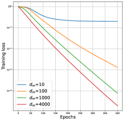
(a)

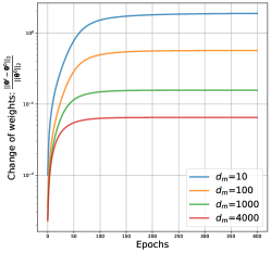
(b)

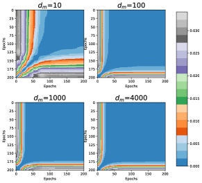
(c)

Figure 2: Visualization of the training process of Transformers with LeCun initialization and $\tau_{0}=d_{m}^{-1/2}$ scaling on synthetic data. (a) Linear convergence. (b) Rate of change of the weights during training. Observe that the weights change very slowly after the $50^{\text{th}}$ epoch. (c) Evolution of the NTK during the training. The result mirrors the plot (b) and demonstrates how the kernel varies significantly at the beginning of the training and remains approximately constant later. As the width increases, the empirical NTK becomes more stable.

Our experiments are organized as follows: In Section 5.1, we conduct experiments with the model Eq. .2 on synthetic data and study the training dynamics. Next, we show convergence results on ViT (Dosovitskiy et al., 2021) on the standard MNIST dataset in Section 5.2. Additional results and detail on the experimental setup are deferred to Appendix E.

5.1 Fitting synthetic data

In this section, we corroborate our theoretical findings on the synthetic data. We generate $100$ data points where the input ${\bm{X}}\in\mathbb{R}^{10\times 100}$ is sampled from standard Gaussian distribution. The corresponding label $y\in\mathbb{R}$ is generated from standard Gaussian distribution. Squared loss is selected as the criterion. We apply gradient descent on the shallow Transformer defined in Eq. .2 with LeCun initialization and $\tau_{0}=d_{m}^{-1/2}$ for $400$ epochs with a fixed step size $\gamma=1$. We test different widths of the network including $d_{m}=\{10,100,1000,4000\}$ and plot the training progress in Figure 2. The result shows that the training can converge except for the case with sub-linear width, see the linear convergence rate in Figure 2(a) and the small movement of the weight in Figure 2(b). For these cases, the weights do not change much after 50 epochs while the losses are still decreasing. In Figure 2(c), we keep track of the evolution of NTK along each epoch. Specifically, the kernel distance is given by:

$$\text{Distance}\left({\bm{K}},\widetilde{{\bm{K}}}\right)=1-\frac{\operatorname{Tr}\left({\bm{K}}\widetilde{{\bm{K}}}^{\top}\right)}{\sqrt{\operatorname{Tr}\left({\bm{K}}{\bm{K}}^{\top}\right)}\sqrt{\operatorname{Tr}\left(\widetilde{{\bm{K}}}\widetilde{{\bm{K}}}^{\top}\right)}}\,,$$

which quantitatively compares two kernels by the relative rotation, as used in Fort et al. (2020). Figure 2(c) shows that the kernel changes rapidly at the beginning of training while being approximately constant at later stages. The experiment with $\tau_{0}=d_{m}^{-1}$, which is deferred to Section E.1, obtains similar results.

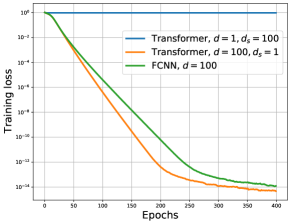
Figure 3: Convergence result on synthetic data with vector input.

Additionally, the experiment with other initialization schemes is deferred to Section E.1, where we observe that NTK initialization indeed yields slower convergence than LeCun/He initialization, which is consistent with our theoretical finding.

Next, in order to verify corollary 1, we feed vector input ${\bm{x}}_{n}\in\mathbb{R}^{100}$ into Transformer by setting either $d_{s}=1,d=100$ or $d_{s}=100,d=1$ under LeCun initialization with $\tau_{0}=d_{m}^{-1}$. Figure 3 shows that the training of Transformer with $d_{s}=1,d=100$ is similar to that of two-layer FCNN with the same width $d_{m}=100$. However, the case of $d_{s}=100,d=1$ fails to converge, which is consistent with our theoretical finding.

5.2 Fitting real-world dataset

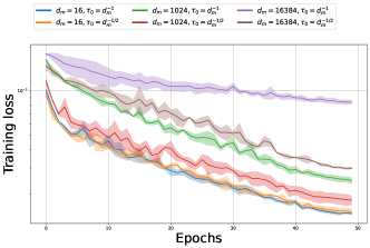
(a)

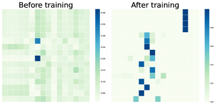
(b)

Figure 4: Convergence curve on MNIST dataset with different scaling schemes and different widths in (a). Visualization of attention map in (b).

Beyond synthetic data, in this section, we examine the convergence performance of Vision Transformer (ViT) on classification task on MNIST dataset (LeCun et al., 1998), which includes 10 classes of images with size $28\times 28$. We use a single layer and single head ViT. The dimension of $d$ is 64. We change the dimension of the query, key, and value from 16 to 1024 and 16384. The network is optimized with SGD with step size $0.1$, and momentum $0.9$ for $50$ epochs. We repeat the experiment for three runs. We present the convergence results over $3$ runs in Figure 4(a), which shows that when the width is smaller, e.g., $16$, both $\tau_{0}=d_{m}^{-1}$ and $\tau_{0}=d_{m}^{-1/2}$ scaling have similar convergence results. However, as the width increases to $1024$ and $16384$, the $\tau_{0}=d_{m}^{-1}$ setting admits a slower rate than that of $\tau_{0}=d_{m}^{-1/2}$, especially a extremely slow rate under $d_{m}=16384$. This is consistent with our theoretical result on the dimension missing effect such that the $\tau_{0}=d_{m}^{-1}$ setting makes Transformer difficult to fit data. Additionally, we visualize the attention map in Figure 4(b), i.e., the output of softmax in the self-attention layer before training and after training under $\tau_{0}=d_{m}^{-1/2}$ setting. We could see that the self-attention layer changes a lot during training.

6 Conclusion

We present a comprehensive analysis of the global convergence properties of shallow Transformer under various scaling and initialization schemes. Regarding scaling schemes, for a large width setting, the difference on convergence between $\tau_{0}=d_{m}^{-1/2}$ and $\tau_{0}=d_{m}^{-1}$ can be demonstrated both theoretically and empirically. Our theory is able to explain this in a dimension missing view. Regarding initialization schemes, our theory prefers to using LeCun and He initialization in Transformer training, which allows for a faster convergence rate than NTK initialization. Though our analysis is limited to shallow Transformers, we believe our framework can be extended to deep Transformers. We provide further discussion into this extension in Section C.7. Exploring the convergence properties of deep Transformers is indeed an intriguing avenue for future research.

Contents of the Appendix

The Appendix is organized as follows:

• In Appendix A, we summarize the symbols and notation used in this work.

• In Section B.1, we provide a theoretical overview for neural tangent kernel (NTK). The background in Sub-Exponential random variables is elaborated in Section B.2. More detailed related work on the convergence analysis of nerual networks can be found in Section B.3.

• The proofs for the convergence of Transformer are included in Appendix C.

• The derivations and the proofs for the NTK are further elaborated in Appendix D, including the formulation of NTK, minimum eigenvalue of NTK, and the relationship between the Hessian and the width.

• Further details on the experiments are developed in Appendix E.

• Limitations and societal impact of this work are discussed in Appendix F and Appendix G, respectively.

Appendix A Symbols and Notation

We include the core symbols and notation in Table 2 for facilitating the understanding of our work.

Table 2: Core symbols and notations used in this paper.

Symbol	Dimension(s)	Definition
$\mathcal{N}(\mu,\sigma)$	-	Gaussian distribution of mean $\mu$ and variance $\sigma$
$\left\|{\bm{w}}\right\|_{2}$	-	Euclidean norms of vectors ${\bm{w}}$
$\left\|{\bm{W}}\right\|_{2}$	-	Spectral norms of matrix ${\bm{W}}$
$\left\|{\bm{W}}\right\|_{\mathrm{F}}$	-	Frobenius norms of matrix ${\bm{W}}$
$\left\|{\bm{W}}\right\|_{\mathrm{\ast}}$	-	Nuclear norms of matrix ${\bm{W}}$
$\lambda_{\min}({\bm{W}}),\lambda_{\max}({\bm{W}})$	-	Minimum and maximum eigenvalues of matrix ${\bm{W}}$
$\sigma_{\min}({\bm{W}}),\sigma_{\max}({\bm{W}})$	-	Minimum and Maximum singular values of matrix ${\bm{W}}$
${\bm{w}}^{(i)}$	-	$i$-th element of vectors ${\bm{w}}$
${\bm{W}}^{(i,j)}$	-	$(i,j)$-th element of matrix ${\bm{W}}$
${\bm{W}}^{t}$	-	${\bm{W}}$ at time step $t$
$\circ$	-	Hadamard product
$\sigma_{s}({\bm{W}})$	-	Row-wise Softmax activation for matrix ${\bm{W}}$
$\sigma_{r}({\bm{W}})$	-	Element-wise ReLU activation for matrix ${\bm{W}}$
$\mathbbm{1}\left\{\text{event}\right\}$	-	Indicator function for event
$N$	-	Size of the dataset
$d_{m}$	-	Width of intermediate layer
$d_{s}$	-	Sequence length of the input
$d$	-	Dimension of each token
$\eta_{Q},\eta_{K},\eta_{V},\eta_{O}$	-	Variance of Gaussian initialization of ${\bm{W}}_{Q},{\bm{W}}_{K},{\bm{W}}_{V},{\bm{w}}_{O}$
$\tau_{0}$, $\tau_{1}$	-	Scaling factor
$\gamma$	-	Step size
${\bm{X}}_{n}$	$\mathbb{R}^{d_{s}\times d}$	The $n$-th data point
$y_{n}$	$\mathbb{R}$	The $n$-th target
$\mathcal{D}_{X}$	-	Input data distribution
$\mathcal{D}_{Y}$	-	Target data distribution
${\bm{\beta}}_{i,n}:=\sigma_{s}\left(\tau_{0}{\bm{X}}_{n}^{(i,:)}{\bm{W}}_{Q}^{\top}{\bm{W}}_{K}{\bm{X}}_{n}^{\top}\right)^{\top}$	$\mathbb{R}^{d_{s}}$	The $i$-th row of the output of softmax of the $n$-th data point
${\bm{y}}:=[y_{1},...,y_{N}]^{\top}$	$\mathbb{R}^{N}$	Ground truth label of the data samples $\{{{\bm{X}}_{n}}\}_{n=1}^{N}$
${\bm{f}}({\bm{\theta}}):=[f({\bm{X}}_{1};{\bm{\theta}}),...,f({\bm{X}}_{N};{\bm{\theta}})]^{\top}$	$\mathbb{R}^{N}$	Network output given data samples $\{{{\bm{X}}_{n}}\}_{n=1}^{N}$
${\bm{F}}_{\text{pre}}({\bm{\theta}}):=[{\bm{a}}_{3}({\bm{X}}_{1};{\bm{\theta}}),...,{\bm{a}}_{3}({\bm{X}}_{N};{\bm{\theta}})]^{\top}$	$\mathbb{R}^{N\times d_{m}}$	Output of the last hidden layer given $\{{{\bm{X}}_{n}}\}_{n=1}^{N}$
$f({\bm{\theta}}):=f({\bm{X}};{\bm{\theta}})$	$\mathbb{R}$	Network output given data samples ${\bm{X}}$
${\bm{f}}_{\text{pre}}:={\bm{a}}_{3}({\bm{X}};{\bm{\theta}})$	$\mathbb{R}^{d_{m}}$	Output of the last hidden layer given${\bm{X}}$
${\bm{W}}_{Q},{\bm{W}}_{K}$	$\mathbb{R}^{d_{m}\times d},\mathbb{R}^{d_{m}\times d}$	Learnable parameters
${\bm{W}}_{V},{\bm{w}}_{O}$	$\mathbb{R}^{d_{m}\times d},\mathbb{R}^{d_{m}}$	Learnable parameters
$\bar{\lambda}_{Q}\triangleq\left\lVert{\bm{W}}_{Q}^{0}\right\rVert_{2}+C_{Q},$ $\bar{\lambda}_{K}\triangleq\left\lVert{\bm{W}}_{K}^{0}\right\rVert_{2}+C_{K}$	$\mathbb{R}$	Parameters norm
$\bar{\lambda}_{V}\triangleq\left\lVert{\bm{W}}_{V}^{0}\right\rVert_{2}+C_{V}$, $\bar{\lambda}_{O}\triangleq\left\lVert{\bm{w}}_{O}^{0}\right\rVert_{2}+C_{O}$	$\mathbb{R}$	Parameters norm
$\rho\triangleq N^{1/2}d_{s}^{3/2}\tau_{1}C_{x},\quad$ $z\triangleq\bar{\lambda}_{O}^{2}\left(1+4\tau_{0}^{2}C_{x}^{4}d_{s}^{2}\bar{\lambda}_{V}^{2}\left(\bar{\lambda}_{Q}^{2}+\bar{\lambda}_{K}^{2}\right)\right)\,$	$\mathbb{R}$	Auxiliary terms
$f_{i}$	$\mathbb{R}$	Output of network for input ${\bm{X}}_{i}$
$\mathcal{O}$, $o$, $\Omega$ and $\Theta$	-	Standard Bachmann–Landau order notation

• * The superscript with bracket represents the element of a vector/matrix, e.g., ${\bm{w}}^{(i)}$ is the $i^{\text{th}}$ element of ${\bm{w}}$.

• * The superscript without bracket symbolizes the parameters at different training steps, e.g., ${\bm{\theta}}^{t}$.

• * The subscript without bracket symbolizes the variable associated to the $n$-th data sample, e.g., ${\bm{X}}_{n}$.

Appendix B Theoretical background

B.1 Preliminary on NTK

In this section, we summarize how training a neural network by minimizing squared loss, i.e., $\ell({\bm{\theta}}^{t})=\frac{1}{2}\sum_{n=1}^{N}(f({\bm{X}}_{n};{\bm{\theta}}^{t})-y_{n})^{2}$, via gradient descent can be characterized by the kernel regression predictor with NTK.

By choosing an infinitesimally small learning rate, we can obtain the following gradient flow:

$$\frac{d{\bm{\theta}}^{t}}{dt}=-\nabla\ell({\bm{\theta}}^{t})\,.$$

By substituting the loss into the above equation and using the chain rule, we can find that the network outputs $f({\bm{\theta}}^{t})\in\mathbb{R}^{N}$ admit the following dynamics:

$$\frac{df({\bm{\theta}}^{t})}{dt}=-{\bm{K}}^{t}(f({\bm{\theta}}^{t})-\bm{y})\,,$$ (5)

where ${\bm{K}}^{t}=\left(\frac{\partial f({\bm{\theta}}^{t})}{\partial{\bm{\theta}}}\right)\left(\frac{\partial f({\bm{\theta}}^{t})}{\partial{\bm{\theta}}}\right)^{\top}\in\mathbb{R}^{N\times N}$. Jacot et al. [2018], Arora et al. [2019b] have shown that for fully-connected neural networks, under the infinite-width setting and proper initialization, ${\bm{K}}^{t}$ will be stable during training and ${\bm{K}}^{0}$ will converge to a fixed matrix $\bm{K}^{\star}\in\mathbb{R}^{N\times N}$, where $({{\bm{K}}}^{\star})^{(ij)}=K^{\star}({\bm{X}}_{i},{\bm{X}}_{j})$ is the NTK value for the inputs ${\bm{X}}_{i}$ and ${\bm{X}}_{j}$. Then, we rewrite Eq. 5 as:

$$\frac{df({\bm{\theta}}^{t})}{dt}=-\bm{K}^{\star}(f({\bm{\theta}}^{t})-\bm{y})\,.$$

This implies the network output for any ${\bm{X}}\in\mathbb{R}^{d_{s}\times d}$ can be calculated by the kernel regression predictor with the associated NTK:

$$f({\bm{X}}) =\left(K^{\star}({\bm{X}},{\bm{X}}_{1}),\cdots,K^{\star}({\bm{X}},{\bm{X}}_{N})\right)\cdot{(\bm{K}^{\star})}^{-1}\bm{y}\,,$$

where $K^{\star}({\bm{X}},{\bm{X}}_{n})$ is the kernel value between test data ${\bm{X}}$ and training data ${\bm{X}}_{n}$.

B.2 Preliminary on Sub-Exponential random variables

Below, we overview the definition of a sub-exponential random variable and few related lemma based on Wainwright [2019]. A random variable $X$ with mean $\mu$ is called sub-exponential random variable if there exist non-negative parameters $(\nu,\alpha)$ such that

$$\mathbb{E}[e^{\lambda(X-\mu)}]\leq e^{\frac{\nu^{2}\lambda^{2}}{2}}\quad\text{ for all }|\lambda|<\frac{1}{\alpha},$$

and we denote by $X\sim SE(\nu,\alpha)$.

Lemma 2.

The multiplication of a scalar $s\in\mathbb{R}^{+}$ and a sub-exponential random variable $X\sim SE(\nu,\alpha)$ is still a sub-exponential random variable: $sX\sim SE(s\nu,s\alpha)$.

Lemma 3.

Given a set of independent sub-exponential random variables $X_{i}\sim(\nu_{i},\alpha_{i})$ for $i\in 1,...,N$, then $\sum_{i=1}^{N}X_{i}\sim(\sqrt{\sum_{i=1}^{N}\nu_{i}^{2}},\max_{i}\alpha_{i})$.

Lemma 4.

Given a sub-exponential random variable $X\sim SE(\nu,\alpha)$ with mean $\mu$, the following inequality holds with probability at least $1-\delta$:

$$|X-\mu|<\max\left(\nu\sqrt{2\log\frac{2}{\delta}},2\alpha\log\frac{2}{\delta}\right)\,.$$

Table 3: Over-parameterization conditions for the convergence analysis of neural network under gradient descent training with squared loss. $L$ is the depth of the network.

	Model	Depth	Initialization	Activation	Width
Allen-Zhu et al. [2019a]	FCNN/CNN	Deep	NTK	ReLU	$\Omega(N^{24}L^{12})$
Du et al. [2019a]	FCNN/CNN	Deep	NTK	Smooth	$\Omega(N^{4}2^{\mathcal{O}(L)})$
Oymak and Soltanolkotabi [2020]	FCNN	Shallow	Standard Gaussian	ReLU	$\Omega(N^{2})$
Zou and Gu [2019]	FCNN	Deep	He	ReLU	$\Omega(N^{8}L^{12})$
Du et al. [2019b]	FCNN	Shallow	NTK	ReLU	$\Omega(N^{6})$
Nguyen [2021]	FCNN	Deep	LeCun	ReLU	$\Omega(N^{3})$
Chen et al. [2021]	FCNN	Deep	NTK	ReLU	$\Omega(L^{22})$
Song et al. [2021]	FCNN	Shallow	He/Lecun	Smooth	$\Omega(N^{3/2})$
Bombari et al. [2022]	FCNN	Deep	He/LeCun	Smooth	$\Omega{(\sqrt{N})}$
Allen-Zhu et al. [2019b]	RNN	-	NTK	ReLU	$\Omega{(N^{c})},c>1$
Hron et al. [2020]	Transformer	Deep	NTK	ReLU	-
Yang [2020]	Transformer	Deep	NTK	Softmax+ReLU	-
Our	Transformer	Shallow	Section 3.2	Softmax+ReLU	$\Omega(N)$

B.3 Related work on over-parameterization for convergence analysis

Recent empirical observation shows that neural networks can fit arbitrary labels with zero training loss when applying the first-order methods, e.g., gradient descent (GD) [Zhang et al., 2017]. Due to the highly non-convex and non-smooth instinct of the neural network, a large body of work have attempted to explain such a phenomenon.

Early work studied the convergence of stochastic gradient descent (SGD) for training two-layer over-parameterized ReLU neural network with cross-entropy loss  [Li and Liang, 2018]. Du et al. [2019b] show that only training the first layer of two-layer ReLU network with square loss by GD can lead to global convergence under the assumption that the Gram matrix is positive definite. Du et al. [2019a] extend the result to deep neural network with smooth activation function and shows that the convergence is guaranteed when the widths of all the hidden layers scale in $\Omega(N^{4})$, where $N$ is the number of data points. Meanwhile, Zou and Gu [2019] prove that the condition for the convergence of GD for deep ReLU network is $\Omega(N^{8})$, which improves upon Allen-Zhu et al. [2019a] that show the result of $\Omega(N^{24})$. Allen-Zhu et al. [2019a] also provide several convergence analyses under the setting of SGD and various loss functions. The assumption regarding the positive definiteness of the Gram matrix made in Du et al. [2019b] has been rigorously proved in Nguyen et al. [2021]. This facilitates Nguyen [2021] to demonstrate that deep ReLU network under LeCUN initialization with width in the order $\Omega{(N^{3})}$ is enough for global convergence. Recent breakthrough [Bombari et al., 2022] improves previous results by showing that sub-linear layer widths suffice for deep neural network with smooth activation function.

Appendix C Proof for convergence analysis

This section is developed for the proof of the convergence result and we outline the flowchart below: Specifically, in Section C.1, we provide some auxiliary lemmas. Lemma 5 and Lemma 6 show that the norm of the parameters can be bounded with high probability at initialization. Lemmas 7, 9 and 10 present that the network output and the output of softmax between two adjacent time steps can be upper bounded. The Lipschitzness of network gradient and its norm is bounded in Lemmas 14 and 13. In Section C.2, we prove the convergence of the general cases, i.e., Proposition. 1. In Sections C.4 and C.3 we present the proof for $d_{m}^{-1/2}$ and $d_{m}^{-1}$ scaling.

C.1 Auxiliary lemmas

Lemma 5 (Corollary 5.35 of Vershynin [2012]).

For a weight matrix ${\bm{W}}\in\mathbb{R}^{d_{1}\times d_{2}}$ where each element is sampled independently from $\mathcal{N}(0,1)$, for every $\zeta\geq 0$, with probability at least $1-2\mathrm{exp}(-\zeta^{2}/2)$ one has:

$$\sqrt{d_{1}}-\sqrt{d_{2}}-\zeta\leq\sigma_{\min}({\bm{W}})\leq\sigma_{\max}({\bm{W}})\leq\sqrt{d_{1}}+\sqrt{d_{2}}+\zeta,$$

where $\sigma_{\max}({\bm{W}})$ and $\sigma_{\min}({\bm{W}})$ represents the maximum and minimum singular value of ${\bm{W}}$, respectively.

Lemma 6 (Upper bound of spectral norms of initial weight).

For a weight matrix ${\bm{W}}\in\mathbb{R}^{d_{m}\times d}$ where $d_{m}>d$ , each element is sampled independently from $\mathcal{N}(0,1)$, with probability at least $1-2\exp(-{d_{m}}/{2})$, one has:

$$\|{\bm{W}}\|_{2}\leq 3\sqrt{d_{m}}.$$

Proof of Lemma 6.

Following Lemma 5, one has:

$$\|\bm{W}\|_{2}\leq\sqrt{d_{m}}+\sqrt{d}+\zeta.$$

Letting $\zeta=\sqrt{d_{m}}$ and using the fact that $d_{m}>d$ complete the proof. ∎

Lemma 7.

Recall from Table 2, ${\bm{\beta}}_{i}=\sigma_{s}\left(\tau_{0}{\bm{X}}^{(i,:)}{\bm{W}}_{Q}^{\top}{\bm{W}}_{K}{\bm{X}}^{\top}\right)^{\top}$ is the $i$-th row of the output of Softmax, if $\max{(\left\lVert{\bm{W}}_{Q}^{t}\right\rVert_{2},\left\lVert{\bm{W}}_{Q}^{t^{\prime}}\right\rVert_{2})}\leq\bar{\lambda}_{Q},\max{(\left\lVert{\bm{W}}_{K}^{t}\right\rVert_{2},\left\lVert{\bm{W}}_{K}^{t^{\prime}}\right\rVert_{2})}\leq\bar{\lambda}_{K},$ then its difference between $t^{\prime}$ step and $t$ step has the following upper bound:

$$\left\lVert{\bm{\beta}}_{i}^{t^{\prime}}-{\bm{\beta}}_{i}^{t}\right\rVert_{2}\leq 2\tau_{0}C_{x}^{2}d_{s}\left(\bar{\lambda}_{Q}\left\lVert{\bm{W}}_{K}^{t^{\prime}}-{\bm{W}}_{K}^{t}\right\rVert_{2}+\bar{\lambda}_{K}\left\lVert{\bm{W}}_{Q}^{t^{\prime}}-{\bm{W}}_{Q}^{t}\right\rVert_{2}\right)\,.$$

Proof.

$$\begin{split}&\left\lVert{\bm{\beta}}_{i}^{t^{\prime}}-{\bm{\beta}}_{i}^{t}\right\rVert_{2}\\ &\leq\left\lVert{\bm{\beta}}_{i}^{t^{\prime}}-{\bm{\beta}}_{i}^{t}\right\rVert_{1}\\ &\leq 2\left\lVert\tau_{0}{\bm{X}}^{(i,:)}{\bm{W}}_{Q}^{t^{\prime}\top}{\bm{W}}_{K}^{t^{\prime}}{\bm{X}}^{\top}-\tau_{0}{\bm{X}}^{(i,:)}{\bm{W}}_{Q}^{t\top}{\bm{W}}_{K}^{t}{\bm{X}}^{\top}\right\rVert_{\infty}\mbox{(By Corollary A.7 in \cite[citet]{\@@bibref{Authors Phrase1YearPhrase2}{edelman2022inductive}{\@@citephrase{[}}{\@@citephrase{]}}})}\\ &=2\max_{j}|\tau_{0}{\bm{X}}^{(i,:)}{\bm{W}}_{Q}^{t^{\prime}\top}{\bm{W}}_{K}^{t^{\prime}}{\bm{X}}^{(j,:)\top}-\tau_{0}{\bm{X}}^{(i,:)}{\bm{W}}_{Q}^{t\top}{\bm{W}}_{K}^{t}{\bm{X}}^{(j,:)\top}|\\ &\leq 2\max_{j}\left(\tau_{0}\left\lVert{\bm{X}}^{(i,:)}\right\rVert_{2}\left\lVert{\bm{W}}_{Q}^{t^{\prime}\top}{\bm{W}}_{K}^{t^{\prime}}-{\bm{W}}_{Q}^{t\top}{\bm{W}}_{K}^{t}\right\rVert_{2}\left\lVert{\bm{X}}^{(j,:)}\right\rVert_{2}\right)\mbox{(By Cauchy-Schwarz inequality)}\\ &\leq 2\tau_{0}C_{x}^{2}d_{s}\left\lVert{\bm{W}}_{Q}^{t^{\prime}\top}{\bm{W}}_{K}^{t^{\prime}}-{\bm{W}}_{Q}^{t\top}{\bm{W}}_{K}^{t}\right\rVert_{2}\mbox{(By \lx@cref{creftype~refnum}{assumption:distribution_1})}\\ &\leq 2\tau_{0}C_{x}^{2}d_{s}\left(\left\lVert{\bm{W}}_{Q}^{t^{\prime}}\right\rVert_{2}\left\lVert{\bm{W}}_{K}^{t^{\prime}}-{\bm{W}}_{K}^{t}\right\rVert_{2}+\left\lVert{\bm{W}}_{K}^{t}\right\rVert_{2}\left\lVert{\bm{W}}_{Q}^{t^{\prime}}-{\bm{W}}_{Q}^{t}\right\rVert_{2}\right)\mbox{(By Cauchy-Schwarz inequality, Triangle inequality)}\\ &\leq 2\tau_{0}C_{x}^{2}d_{s}\left(\bar{\lambda}_{Q}\left\lVert{\bm{W}}_{K}^{t^{\prime}}-{\bm{W}}_{K}^{t}\right\rVert_{2}+\bar{\lambda}_{K}\left\lVert{\bm{W}}_{Q}^{t^{\prime}}-{\bm{W}}_{Q}^{t}\right\rVert_{2}\right)\,.\end{split}$$

∎

Lemma 8 (Upper bound the Euclidean norm of the output of softmax).

Suppose ${\bm{v}}=\textnormal{Softmax}({\bm{u}})\in\mathbb{R}^{d_{s}}$, then one has: $1/\sqrt{d_{s}}\leq\left\lVert{\bm{v}}\right\rVert_{2}\leq 1\,.$

Proof.

By the inequality of arithmetic and geometric mean:

$$\frac{1}{\sqrt{d_{s}}}=\frac{\sum_{i=1}^{d_{s}}{\bm{v}}^{(i)}}{\sqrt{d_{s}}}\leq\left\lVert{\bm{v}}\right\rVert_{2}=\sqrt{\sum_{i=1}^{d_{s}}\left(({\bm{v}}^{(i)})^{2}\right)}\leq\sqrt{\left(\sum_{i=1}^{d_{s}}({\bm{v}}^{(i)})\right)^{2}}=1\,.$$

∎

Lemma 9.

If at $t^{\prime}$ and $t$ step, $\max{(\left\lVert{\bm{W}}_{Q}^{t}\right\rVert_{2},\left\lVert{\bm{W}}_{Q}^{t^{\prime}}\right\rVert_{2})}\leq\bar{\lambda}_{Q},\max{(\left\lVert{\bm{W}}_{K}^{t}\right\rVert_{2},\left\lVert{\bm{W}}_{K}^{t^{\prime}}\right\rVert_{2})}\leq\bar{\lambda}_{K},\max{(\left\lVert{\bm{W}}_{V}^{t}\right\rVert_{2},\left\lVert{\bm{W}}_{V}^{t^{\prime}}\right\rVert_{2})}\leq\bar{\lambda}_{V}$, then the difference between the output of the last hidden layer at $t^{\prime}$ step and $t$ can be upper bounded by:

$$\left\lVert{\bm{F}}_{\text{pre}}^{t^{\prime}}-{\bm{F}}_{\text{pre}}^{t}\right\rVert_{\mathrm{F}}\leq\rho\left(\left\lVert{\bm{W}}_{V}^{t^{\prime}}-{\bm{W}}_{V}^{t}\right\rVert_{2}+\bar{\lambda}_{V}2\tau_{0}C_{x}^{2}d_{s}\left(\bar{\lambda}_{Q}\left\lVert{\bm{W}}_{K}^{t^{\prime}}-{\bm{W}}_{K}^{t}\right\rVert_{2}+\bar{\lambda}_{K}\left\lVert{\bm{W}}_{Q}^{t^{\prime}}-{\bm{W}}_{Q}^{t}\right\rVert_{2}\right)\right)\,.$$

Proof.

Note that ${\bm{F}}_{\text{pre}}\in\mathbb{R}^{N\times d_{m}}$ is the output of the last hidden layer given $\{{{\bm{X}}_{n}}\}_{n=1}^{N}$ sample as defined in Table 2. We firstly analyze each sample, i.e., ${\bm{f}}_{\text{pre}}\in\mathbb{R}^{d_{m}}$ and we drop the index $n$ for simplification.

$$\begin{split}&\left\lVert{\bm{f}}_{\text{pre}}^{t^{\prime}}-{\bm{f}}_{\text{pre}}^{t}\right\rVert_{2}=\tau_{1}\left\lVert\sum_{i=1}^{d_{s}}\sigma_{r}\left({\bm{W}}_{V}^{t^{\prime}}{\bm{X}}^{\top}{\bm{\beta}}_{i}^{t^{\prime}}\right)-\sum_{i=1}^{d_{s}}\sigma_{r}\left({\bm{W}}_{V}^{t}{\bm{X}}^{\top}{\bm{\beta}}_{i}^{t}\right)\right\rVert_{2}\\ &\leq\tau_{1}\sum_{i=1}^{d_{s}}\left\lVert{\bm{W}}_{V}^{t^{\prime}}{\bm{X}}^{\top}{\bm{\beta}}_{i}^{t^{\prime}}-{\bm{W}}_{V}^{t}{\bm{X}}^{\top}{\bm{\beta}}_{i}^{t}\right\rVert_{2}\mbox{(By Lipschitz continuity of $\sigma_{r}$)}\\ &\leq\tau_{1}\sum_{i=1}^{d_{s}}\left(\left\lVert({\bm{W}}_{V}^{t^{\prime}}-{\bm{W}}_{V}^{t}){\bm{X}}^{\top}{\bm{\beta}}_{i}^{t^{\prime}}\right\rVert_{2}+\left\lVert{\bm{W}}_{V}^{t}{\bm{X}}({\bm{\beta}}_{i}^{t^{\prime}}-{\bm{\beta}}_{i}^{t})\right\rVert_{2}\right)\mbox{(By Triangle inequality)}\\ &\leq\tau_{1}\sum_{i=1}^{d_{s}}\left(\left\lVert{\bm{W}}_{V}^{t^{\prime}}-{\bm{W}}_{V}^{t}\right\rVert_{2}\left\lVert{\bm{X}}\right\rVert_{2}\left\lVert{\bm{\beta}}_{i}^{t^{\prime}}\right\rVert_{2}+\left\lVert{\bm{W}}_{V}^{t}\right\rVert_{2}\left\lVert{\bm{X}}\right\rVert_{2}\left\lVert{\bm{\beta}}_{i}^{t^{\prime}}-{\bm{\beta}}_{i}^{t}\right\rVert_{2}\right)\mbox{(By Cauchy-Schwarz inequality)}\\ &\leq\tau_{1}C_{x}\sqrt{d_{s}}\sum_{i=1}^{d_{s}}\left(\left\lVert{\bm{W}}_{V}^{t^{\prime}}-{\bm{W}}_{V}^{t}\right\rVert_{2}+\bar{\lambda}_{V}\left\lVert{\bm{\beta}}_{i}^{t^{\prime}}-{\bm{\beta}}_{i}^{t}\right\rVert_{2}\right)\mbox{ (By \lx@cref{creftype~refnum}{lemma:softmaxbound} and \lx@cref{creftype~refnum}{assumption:distribution_1}) }\\ &\leq\tau_{1}C_{x}d_{s}^{3/2}\left(\left\lVert{\bm{W}}_{V}^{t^{\prime}}-{\bm{W}}_{V}^{t}\right\rVert_{2}+\bar{\lambda}_{V}2\tau_{0}C_{x}^{2}d_{s}\left(\bar{\lambda}_{Q}\left\lVert{\bm{W}}_{K}^{t^{\prime}}-{\bm{W}}_{K}^{t}\right\rVert_{2}+\bar{\lambda}_{K}\left\lVert{\bm{W}}_{Q}^{t^{\prime}}-{\bm{W}}_{Q}^{t}\right\rVert_{2}\right)\right)\mbox{ (By \lx@cref{creftype~refnum}{lemma:lipsoftmax}) }.\end{split}$$ (6)

Next, we bound the difference given $N$ data sample:

$$\left\lVert{\bm{F}}_{\text{pre}}^{t^{\prime}}-{\bm{F}}_{\text{pre}}^{t}\right\rVert_{\mathrm{F}}\leq\sqrt{N}\tau_{1}C_{x}d_{s}^{3/2}\left(\left\lVert{\bm{W}}_{V}^{t^{\prime}}-{\bm{W}}_{V}^{t}\right\rVert_{2}+\bar{\lambda}_{V}2\tau_{0}C_{x}^{2}d_{s}\left(\bar{\lambda}_{Q}\left\lVert{\bm{W}}_{K}^{t^{\prime}}-{\bm{W}}_{K}^{t}\right\rVert_{2}+\bar{\lambda}_{K}\left\lVert{\bm{W}}_{Q}^{t^{\prime}}-{\bm{W}}_{Q}^{t}\right\rVert_{2}\right)\right)$$

$$=\rho\left(\left\lVert{\bm{W}}_{V}^{t^{\prime}}-{\bm{W}}_{V}^{t}\right\rVert_{2}+\bar{\lambda}_{V}2\tau_{0}C_{x}^{2}d_{s}\left(\bar{\lambda}_{Q}\left\lVert{\bm{W}}_{K}^{t^{\prime}}-{\bm{W}}_{K}^{t}\right\rVert_{2}+\bar{\lambda}_{K}\left\lVert{\bm{W}}_{Q}^{t^{\prime}}-{\bm{W}}_{Q}^{t}\right\rVert_{2}\right)\right)\,,$$

where the last equality is by the definition of $\rho$ in Proposition. 1. ∎

Lemma 10.

If at $t^{\prime}$ and $t$ step, $\max{(\left\lVert{\bm{W}}_{Q}^{t}\right\rVert_{2},\left\lVert{\bm{W}}_{Q}^{t^{\prime}}\right\rVert_{2})}\leq\bar{\lambda}_{Q},\max{(\left\lVert{\bm{W}}_{K}^{t}\right\rVert_{2},\left\lVert{\bm{W}}_{K}^{t^{\prime}}\right\rVert_{2})}\leq\bar{\lambda}_{K},\max{(\left\lVert{\bm{W}}_{V}^{t}\right\rVert_{2},\left\lVert{\bm{W}}_{V}^{t^{\prime}}\right\rVert_{2})}\leq\bar{\lambda}_{V},\max{(\left\lVert{\bm{w}}_{O}^{t}\right\rVert_{2},\left\lVert{\bm{w}}_{O}^{t^{\prime}}\right\rVert_{2})}\leq\bar{\lambda}_{O}$, then the difference between the network output at $t^{\prime}$ step and $t$ step can be upper bounded by:

$$\begin{split}&\left\lVert{\bm{f}}^{t^{\prime}}-{\bm{f}}^{t}\right\rVert_{2}\leq\rho\bar{\lambda}_{V}\left\lVert{\bm{w}}_{O}^{t^{\prime}}-{\bm{w}}_{O}^{t}\right\rVert_{2}+\bar{\lambda}_{O}\left\lVert{\bm{F}}_{\mathrm{pre}}^{t^{\prime}}-{\bm{F}}_{\mathrm{pre}}^{t}\right\rVert_{\mathrm{F}}\,.\end{split}$$

Proof.

$$\begin{split}&\left\lVert{\bm{f}}^{t^{\prime}}-{\bm{f}}^{t}\right\rVert_{2}=\left\lVert{\bm{F}}^{t^{\prime}}_{\mathrm{pre}}{\bm{w}}_{O}^{t^{\prime}}-{\bm{F}}^{t}_{\mathrm{pre}}{\bm{w}}_{O}^{t}\right\rVert_{2}\leq\left\lVert{\bm{F}}^{t^{\prime}}_{\mathrm{pre}}\right\rVert_{2}\left\lVert{\bm{w}}_{O}^{t^{\prime}}-{\bm{w}}_{O}^{t}\right\rVert_{2}+\left\lVert{\bm{w}}_{O}^{t}\right\rVert_{2}\left\lVert{\bm{F}}^{t^{\prime}}_{\mathrm{pre}}-{\bm{F}}^{t}_{\mathrm{pre}}\right\rVert_{2}\,,\end{split}$$

where we use triangle inequality. Then, the first term of the RHS can be bounded by:

$$\left\lVert{\bm{F}}^{t^{\prime}}_{\mathrm{pre}}\right\rVert_{2}\leq\left\lVert{\bm{F}}^{t^{\prime}}_{\mathrm{pre}}\right\rVert_{\mathrm{F}}=\left\lVert\begin{bmatrix}\tau_{1}\sum_{i=1}^{d_{s}}\sigma_{r}\left({\bm{W}}_{V}^{t^{\prime}}{\bm{X}}_{1}^{\top}{\bm{\beta}}_{i,1}^{t^{\prime}}\right)\\ \vdots\\ \tau_{1}\sum_{i=1}^{d_{s}}\sigma_{r}\left({\bm{W}}_{V}^{t^{\prime}}{\bm{X}}_{N}^{\top}{\bm{\beta}}_{i,N}^{t^{\prime}}\right)\end{bmatrix}\right\rVert_{\mathrm{F}}\leq\tau_{1}\sqrt{N}d_{s}^{3/2}C_{x}\left\lVert{\bm{W}}_{V}^{t^{\prime}}\right\rVert_{2}=\rho\left\lVert{\bm{W}}_{V}^{t^{\prime}}\right\rVert_{2}\,,$$

where the last equality is by the definition of $\rho$ in Proposition. 1. ∎

Lemma 11 (Jacobian of Softmax).

Suppose ${\bm{v}}=\textnormal{Softmax}({\bm{u}})\in\mathbb{R}^{d_{s}}$, then $\frac{\partial{\bm{v}}}{\partial{\bm{u}}}=\textnormal{diag}({\bm{v}})-{\bm{v}}{\bm{v}}^{\top}$.

Proof.

We can reformulate $\bm{v}$ as: ${\bm{v}}=\begin{bmatrix}\frac{\exp{({\bm{u}}^{(1)})}}{\sum_{i=1}^{d_{s}}\exp{({\bm{u}}^{(i)})}}\\ \vdots\\ \frac{\exp{({\bm{u}}^{(d_{s})})}}{\sum_{i=1}^{d_{s}}\exp{({\bm{u}}^{(i)})}}\end{bmatrix}.$

Then, we have

$$\begin{split}\frac{\partial{\bm{v}}^{(j)}}{\partial{\bm{u}}^{(k)}}=\frac{\partial\frac{\exp{({\bm{u}}^{(j)})}}{\sum_{i=1}^{d_{s}}\exp{({\bm{u}}^{(i)})}}}{\partial{\bm{u}}^{(k)}}&=\left\{\begin{array}[]{ll}\frac{-\exp{({\bm{u}}^{(j)})}-\exp{({\bm{u}}^{(k)})}}{(\sum_{i=1}^{d_{s}}\exp{({\bm{u}}^{(i)})})^{2}}&\mbox{if }j\neq k\\ \frac{\exp{({\bm{u}}^{(k)})}\sum_{i=1}^{d_{s}}\exp{({\bm{u}}^{(i)})}-(\exp{({\bm{u}}^{(k)})})^{2}}{\left(\sum_{i=1}^{d_{s}}\exp{({\bm{u}}^{(i)})}\right)^{2}}&\mbox{if }j=k\end{array}\right.\\ &=\left\{\begin{array}[]{ll}-{\bm{v}}^{(j)}{\bm{v}}^{(k)}&\mbox{if }j\neq k\\ {\bm{v}}^{(k)}-{\bm{v}}^{(j)}{\bm{v}}^{(k)}&\mbox{if }j=k\end{array}\right.\end{split}$$

Thus

$$\begin{split}\frac{\partial\bm{v}}{\partial\mathbf{u}}=\textnormal{diag}(\bm{v})-\bm{v}\bm{v}^{\top}\,.\end{split}$$

∎

Lemma 12 (Upper bound for the loss gradient norm).

If $\left\lVert{\bm{W}}_{Q}^{t}\right\rVert_{2}\leq\bar{\lambda}_{Q},\left\lVert{\bm{W}}_{K}^{t}\right\rVert_{2}\leq\bar{\lambda}_{K},\left\lVert{\bm{W}}_{V}^{t}\right\rVert_{2}\leq\bar{\lambda}_{V},\left\lVert{\bm{w}}_{O}^{t}\right\rVert_{2}\leq\bar{\lambda}_{O},$ then the gradient norm with respect to ${\bm{W}}_{Q},{\bm{W}}_{K},{\bm{W}}_{V},{\bm{w}}_{O}$ can be upper bounded by:

$$\begin{split}&\left\lVert\nabla_{{\bm{W}}_{Q}}\ell({\bm{\theta}}^{\top})\right\rVert_{\mathrm{F}}\leq 2\rho\tau_{0}\bar{\lambda}_{K}\bar{\lambda}_{V}\bar{\lambda}_{O}d_{s}C_{x}^{2}\left\lVert{\bm{f}}^{t}-{\bm{y}}\right\rVert_{2}\,,\quad\quad\left\lVert\nabla_{{\bm{W}}_{K}}\ell({\bm{\theta}}^{\top})\right\rVert_{\mathrm{F}}\leq 2\rho\tau_{0}\bar{\lambda}_{Q}\bar{\lambda}_{V}\bar{\lambda}_{O}d_{s}C_{x}^{2}\left\lVert{\bm{f}}^{t}-{\bm{y}}\right\rVert_{2}\,,\\ &\left\lVert\nabla_{{\bm{W}}_{V}}\ell({\bm{\theta}}^{\top})\right\rVert_{\mathrm{F}}\leq\rho\bar{\lambda}_{O}\left\lVert{\bm{f}}^{t}-{\bm{y}}\right\rVert_{2}\,,\qquad\qquad\qquad\qquad\left\lVert\nabla_{{\bm{w}}_{O}}\ell({\bm{\theta}}^{\top})\right\rVert_{2}\leq\rho\bar{\lambda}_{V}\left\lVert{\bm{f}}^{t}-{\bm{y}}\right\rVert_{2}\,.\end{split}$$

Proof.

To simplify the notation, in the proof below, we hide the index $t$. Firstly, consider the gradient w.r.t ${\bm{W}}_{V}$,

$$\begin{split}&\left\lVert\nabla_{{\bm{W}}_{V}}\ell({\bm{\theta}})\right\rVert_{\mathrm{F}}=\left\lVert-\sum^{N}_{n=1}(f({\bm{X}}_{n})-y_{n})\frac{\partial f({\bm{X}}_{n})}{\partial{\bm{W}}_{V}}\right\rVert_{\mathrm{F}}\\ &=\tau_{1}\left\lVert\sum^{N}_{n=1}(f({\bm{X}}_{n})-y_{n})\sum_{i=1}^{d_{s}}\left({\bm{w}}_{O}\circ\dot{\sigma_{r}}\left({\bm{W}}_{V}{\bm{X}}_{n}^{\top}{\bm{\beta}}_{i,n}\right)\right){\bm{\beta}}_{i,n}^{\top}{\bm{X}}_{n}\ \right\rVert_{\mathrm{F}}\leq\tau_{1}\sum^{N}_{n=1}\left|(f({\bm{X}}_{n})-y_{n})\right|d_{s}^{3/2}\bar{\lambda}_{O}C_{x}\\ &\leq\tau_{1}\sqrt{N\sum^{N}_{n=1}\left|(f({\bm{X}}_{n})-y_{n})\right|^{2}}d_{s}^{3/2}\bar{\lambda}_{O}C_{x}=\tau_{1}d_{s}^{3/2}\bar{\lambda}_{O}C_{x}\sqrt{N}\left\lVert{\bm{f}}-{\bm{y}}\right\rVert_{2}=\rho\bar{\lambda}_{O}\left\lVert{\bm{f}}-{\bm{y}}\right\rVert_{2}\,,\end{split}$$ (7)

where the last equality is by the definition of $\rho$ in Proposition. 1. Next, consider the gradient w.r.t ${\bm{w}}_{O}$,

$$\begin{split}&\left\lVert\nabla_{{\bm{w}}_{O}}\ell({\bm{\theta}})\right\rVert_{2}=\left\lVert-\sum^{N}_{n=1}(f({\bm{X}}_{n})-y_{n})\frac{\partial f({\bm{X}}_{n})}{\partial{\bm{w}}_{O}}\right\rVert_{2}=\tau_{1}\left\lVert\sum^{N}_{n=1}(f({\bm{X}}_{n})-y_{n})\sum_{i=1}^{d_{s}}\sigma_{r}\left({\bm{W}}_{V}{\bm{X}}_{n}^{\top}{\bm{\beta}}_{i,n}\right)\right\rVert_{2}\\ &\leq\tau_{1}\sum^{N}_{n=1}\left|(f({\bm{X}}_{n})-y_{n})\right|d_{s}^{3/2}\bar{\lambda}_{V}C_{x}\leq\tau_{1}\sqrt{N\sum^{N}_{n=1}\left|(f({\bm{X}}_{n})-y_{n})\right|^{2}}d_{s}^{3/2}\bar{\lambda}_{V}C_{x}=\rho\bar{\lambda}_{V}\left\lVert{\bm{f}}-{\bm{y}}\right\rVert_{2}\,,\end{split}$$ (8)

Next, consider the gradient w.r.t ${\bm{W}}_{Q}$,

$$\begin{split}&\left\lVert\nabla_{{\bm{W}}_{Q}}\ell({\bm{\theta}})\right\rVert_{\mathrm{F}}=\left\lVert-\sum^{N}_{n=1}(f({\bm{X}}_{n})-y_{n})\frac{\partial f({\bm{X}}_{n})}{\partial{\bm{W}}_{Q}}\right\rVert_{\mathrm{F}}\\ &=\tau_{0}\tau_{1}\left\lVert\sum^{N}_{n=1}(f({\bm{X}}_{n})-y_{n})\sum_{i=1}^{d_{s}}{\bm{W}}_{k}{\bm{X}}_{n}^{\top}\left(\mathrm{diag}({\bm{\beta}}_{i,n})-{\bm{\beta}}_{i,n}{\bm{\beta}}_{i,n}^{\top}\right){\bm{X}}_{n}{\bm{W}}_{V}^{\top}\left({\bm{w}}_{O}\circ\dot{\sigma_{r}}\left({\bm{W}}_{V}{\bm{X}}_{n}^{\top}{\bm{\beta}}_{i,n}\right)\right){\bm{X}}_{n}^{(i,:)}\right\rVert_{\mathrm{F}}\\ &\leq 2\tau_{0}\tau_{1}\sum^{N}_{n=1}\left|(f({\bm{X}}_{n})-y_{n})\right|d_{s}\bar{\lambda}_{K}\bar{\lambda}_{V}\bar{\lambda}_{O}(C_{x}\sqrt{d_{s}})^{3}\\ &\leq 2\tau_{0}\tau_{1}\sqrt{N\sum^{N}_{n=1}\left|(f({\bm{X}}_{n})-y_{n})\right|^{2}}d_{s}\bar{\lambda}_{K}\bar{\lambda}_{V}\bar{\lambda}_{O}(C_{x}\sqrt{d_{s}})^{3}\\ &=2\rho\tau_{0}\bar{\lambda}_{K}\bar{\lambda}_{V}\bar{\lambda}_{O}d_{s}C_{x}^{2}\left\lVert{\bm{f}}-{\bm{y}}\right\rVert_{2}\,.\end{split}$$ (9)

Similarly, for the gradient w.r.t ${\bm{W}}_{K}$, we have:

$$\left\lVert\nabla_{{\bm{W}}_{K}}\ell({\bm{\theta}})\right\rVert_{\mathrm{F}}\leq 2\rho\tau_{0}\bar{\lambda}_{Q}\bar{\lambda}_{V}\bar{\lambda}_{O}d_{s}C_{x}^{2}\left\lVert{\bm{f}}-{\bm{y}}\right\rVert_{2}\,.$$ (10)

∎

Lemma 13 (Upper bound for the network function gradient norm).

If $\left\lVert{\bm{W}}_{Q}^{t}\right\rVert_{2}\leq\bar{\lambda}_{Q},\left\lVert{\bm{W}}_{K}^{t}\right\rVert_{2}\leq\bar{\lambda}_{K},\left\lVert{\bm{W}}_{V}^{t}\right\rVert_{2}\leq\bar{\lambda}_{V},\left\lVert{\bm{w}}_{O}^{t}\right\rVert_{2}\leq\bar{\lambda}_{O},$ then one has:

$$\begin{split}\left\lVert\nabla_{\bm{\theta}}{\bm{f}}^{t}\right\rVert_{2}\leq c_{2}\,,\end{split}$$

where

$$c_{2}\triangleq\rho\sqrt{\bar{\lambda}_{O}^{2}+\bar{\lambda}_{V}^{2}+(2\tau_{0}\bar{\lambda}_{K}\bar{\lambda}_{V}\bar{\lambda}_{O}d_{s}C_{x}^{2})^{2}+(2\tau_{0}\bar{\lambda}_{Q}\bar{\lambda}_{V}\bar{\lambda}_{O}d_{s}C_{x}^{2})^{2}}\,.$$ (11)

Proof.

To simplify the notation, in the proof below, we hide the index $t$. Firstly, note that:

$$\begin{split}&\left\lVert\nabla_{\bm{\theta}}{\bm{f}}\right\rVert_{2}\leq\left\lVert\nabla_{\bm{\theta}}{\bm{f}}\right\rVert_{\mathrm{F}}\\ &=\sqrt{\sum_{n=1}^{N}\left(\left\lVert\nabla_{{\bm{w}}_{O}}f({\bm{X}}_{n};{\bm{\theta}})\right\rVert_{2}^{2}+\left\lVert\nabla_{{\bm{w}}_{Q}}f({\bm{X}}_{n};{\bm{\theta}})\right\rVert_{\mathrm{F}}^{2}+\left\lVert\nabla_{{\bm{w}}_{K}}f({\bm{X}}_{n};{\bm{\theta}})\right\rVert_{\mathrm{F}}^{2}+\left\lVert\nabla_{{\bm{W}}_{V}}f({\bm{X}}_{n};{\bm{\theta}})\right\rVert_{\mathrm{F}}^{2}\right)}.\end{split}$$ (12)

Then following the step as in Eqs. 8, 7, 10 and 9, each term can be bounded as follows:

$$\begin{split}&\sum_{n=1}^{N}\left(\left\lVert\nabla_{{\bm{W}}_{V}}f({\bm{X}}_{n};{\bm{\theta}})\right\rVert_{\mathrm{F}}^{2}\right)\leq(\rho\bar{\lambda}_{O})^{2},\qquad\qquad\qquad\quad\sum_{n=1}^{N}\left(\left\lVert\nabla_{{\bm{w}}_{O}}f({\bm{X}}_{n};{\bm{\theta}})\right\rVert_{2}\right)\leq(\rho\bar{\lambda}_{V})^{2}\,,\\ &\sum_{n=1}^{N}\left(\left\lVert\nabla_{{\bm{w}}_{Q}}f({\bm{X}}_{n};{\bm{\theta}})\right\rVert_{\mathrm{F}}\right)\leq(2\rho\tau_{0}\bar{\lambda}_{K}\bar{\lambda}_{V}\bar{\lambda}_{O}d_{s}C_{x}^{2})^{2},\quad\sum_{n=1}^{N}\left(\left\lVert\nabla_{{\bm{w}}_{K}}f({\bm{X}}_{n};{\bm{\theta}})\right\rVert_{\mathrm{F}}\right)\leq(2\rho\tau_{0}\bar{\lambda}_{Q}\bar{\lambda}_{V}\bar{\lambda}_{O}d_{s}C_{x}^{2})^{2}\,.\end{split}$$

Plugging these bounds back LABEL:equ:gradientallbound finishes the proof. ∎

Lemma 14 (Upper bound for the Lipschitzness of the network gradient).

Suppose $\max{(\left\lVert{\bm{W}}_{Q}^{t}\right\rVert_{2},\left\lVert{\bm{W}}_{Q}^{t^{\prime}}\right\rVert_{2})}\leq\bar{\lambda}_{Q},\max{(\left\lVert{\bm{W}}_{K}^{t}\right\rVert_{2},\left\lVert{\bm{W}}_{K}^{t^{\prime}}\right\rVert_{2})}\leq\bar{\lambda}_{K},\max{(\left\lVert{\bm{W}}_{V}^{t}\right\rVert_{2},\left\lVert{\bm{W}}_{V}^{t^{\prime}}\right\rVert_{2})}\leq\bar{\lambda}_{V},\max{(\left\lVert{\bm{w}}_{O}^{t}\right\rVert_{2},\left\lVert{\bm{w}}_{O}^{t^{\prime}}\right\rVert_{2})}\leq\bar{\lambda}_{O},$ and define $z\triangleq 2\tau_{0}C_{x}^{2}d_{s}(\bar{\lambda}_{Q}+\bar{\lambda}_{K})$, then one has

$$\left\lVert\nabla_{\bm{\theta}}{\bm{f}}^{t^{\prime}}-\nabla_{\bm{\theta}}{\bm{f}}^{t}\right\rVert_{2}\leq c_{3}\left\lVert{\bm{\theta}}^{t^{\prime}}-{\bm{\theta}}^{t}\right\rVert_{2}\,,$$ (13)

where

$$\begin{split}&(c_{3})^{2}\triangleq N(\tau_{1}C_{x}d_{s}^{3/2}(1+\bar{\lambda}_{V}z))^{2}\\ &\quad+N\left\{\tau_{1}C_{x}d_{s}^{3/2}\bigg{[}\bar{\lambda}_{O}z+\bar{\lambda}_{O}C_{x}\sqrt{d_{s}}(1+\bar{\lambda}_{V}z)+1\bigg{]}\right\}^{2}\\ &\quad+N\left\{\tau_{0}\tau_{1}C_{x}d_{s}\left\{2\bar{\lambda}_{K}d_{s}C_{x}^{2}\left[\bar{\lambda}_{V}\left(\bar{\lambda}_{O}C_{x}\sqrt{d_{s}}(1+\bar{\lambda}_{V}z)+1\right)+\bar{\lambda}_{O}\right]+\bar{\lambda}_{V}\bar{\lambda}_{O}[C_{x}^{2}d_{s}+3\bar{\lambda}_{K}z]\right\}\right\}^{2}\\ &\quad+N\left\{\tau_{0}\tau_{1}C_{x}d_{s}\left\{2\bar{\lambda}_{Q}d_{s}C_{x}^{2}\left[\bar{\lambda}_{V}\left(\bar{\lambda}_{O}C_{x}\sqrt{d_{s}}(1+\bar{\lambda}_{V}z)+1\right)+\bar{\lambda}_{O}\right]+\bar{\lambda}_{V}\bar{\lambda}_{O}[C_{x}^{2}d_{s}+3\bar{\lambda}_{K}z]\right\}\right\}^{2}\,.\end{split}$$ (14)

Proof.

Firstly, note that:

$$\begin{split}&\left\lVert\nabla_{\bm{\theta}}{\bm{f}}^{t^{\prime}}-\nabla_{\bm{\theta}}{\bm{f}}^{t}\right\rVert_{2}^{2}\\ &\leq\sum_{n=1}^{N}\left(\left\lVert\nabla_{{\bm{w}}_{O}}f({\bm{X}}_{n};{\bm{\theta}}^{t^{\prime}})-\nabla_{{\bm{w}}_{O}}f({\bm{X}}_{n};{\bm{\theta}}^{t})\right\rVert_{2}^{2}+\left\lVert\nabla_{{\bm{W}}_{V}}f({\bm{X}}_{n};{\bm{\theta}}^{t^{\prime}})-\nabla_{{\bm{W}}_{V}}f({\bm{X}}_{n};{\bm{\theta}}^{t})\right\rVert_{\mathrm{F}}^{2}\right.\\ &\qquad\left.+\left\lVert\nabla_{{\bm{W}}_{Q}}f({\bm{X}}_{n};{\bm{\theta}}^{t^{\prime}})-\nabla_{{\bm{W}}_{Q}}f({\bm{X}}_{n};{\bm{\theta}}^{t})\right\rVert_{\mathrm{F}}^{2}+\left\lVert\nabla_{{\bm{W}}_{K}}f({\bm{X}}_{n};{\bm{\theta}}^{t^{\prime}})-\nabla_{{\bm{W}}_{K}}f({\bm{X}}_{n};{\bm{\theta}}^{t})\right\rVert_{\mathrm{F}}^{2}\right)\,.\end{split}$$ (15)

Then, we will prove each term separately. Regarding the first term in Eq. 15, we have

$$\begin{split}&\left\lVert\nabla_{{\bm{w}}_{O}}f({\bm{X}}_{n};{\bm{\theta}}^{t^{\prime}})-\nabla_{{\bm{w}}_{O}}f({\bm{X}}_{n};{\bm{\theta}}^{t})\right\rVert_{2}\\ &=\left\lVert{\bm{f}}_{\text{pre}}^{t^{\prime}}-{\bm{f}}_{\text{pre}}^{t}\right\rVert_{2}\\ &\leq\tau_{1}C_{x}d_{s}^{3/2}\left(\left\lVert{\bm{W}}_{V}^{t^{\prime}}-{\bm{W}}_{V}^{t}\right\rVert_{2}+\bar{\lambda}_{V}2\tau_{0}C_{x}^{2}d_{s}\left(\bar{\lambda}_{Q}\left\lVert{\bm{W}}_{K}^{t^{\prime}}-{\bm{W}}_{K}^{t}\right\rVert_{2}+\bar{\lambda}_{K}\left\lVert{\bm{W}}_{Q}^{t^{\prime}}-{\bm{W}}_{Q}^{t}\right\rVert_{2}\right)\right)\\ &\leq\tau_{1}C_{x}d_{s}^{3/2}\left(1+\bar{\lambda}_{V}2\tau_{0}C_{x}^{2}d_{s}\left(\bar{\lambda}_{Q}+\bar{\lambda}_{K}\right)\right)\left\lVert{\bm{\theta}}^{t^{\prime}}-{\bm{\theta}}^{t}\right\rVert_{2}\\ &=\tau_{1}C_{x}d_{s}^{3/2}(1+\bar{\lambda}_{V}z)\left\lVert{\bm{\theta}}^{t^{\prime}}-{\bm{\theta}}^{t}\right\rVert_{2}\,.\end{split}$$ (16)

where the first inequality is by Eq. 6, and in the last equality is by the definition of $z$ in the lemma. Regarding the second term in Eq. 15, we have:

$$\small\begin{split}&\left\lVert\nabla_{{\bm{W}}_{V}}f({\bm{X}}_{n};{\bm{\theta}}^{t^{\prime}})-\nabla_{{\bm{W}}_{V}}f({\bm{X}}_{n};{\bm{\theta}}^{t})\right\rVert_{\mathrm{F}}\\ &=\tau_{1}\left\lVert\sum_{i=1}^{d_{s}}\left({\bm{w}}_{O}^{t^{\prime}}\circ\dot{\sigma_{r}}\left({\bm{W}}_{V}^{t^{\prime}}{\bm{X}}_{n}^{\top}{\bm{\beta}}_{i,n}^{t^{\prime}}\right)\right){{\bm{\beta}}_{i,n}^{t^{\prime}}}^{\top}{\bm{X}}_{n}-\sum_{i=1}^{d_{s}}\left({\bm{w}}_{O}^{t}\circ\dot{\sigma_{r}}\left({\bm{W}}_{V}^{t}{\bm{X}}_{n}^{\top}{\bm{\beta}}_{i,n}^{t}\right)\right){{\bm{\beta}}_{i,n}^{t}}^{\top}{\bm{X}}_{n}\right\rVert_{\text{F}}\\ &\leq\tau_{1}C_{x}\sqrt{d_{s}}\sum_{i=1}^{d_{s}}\left\lVert\left({\bm{w}}_{O}^{t^{\prime}}\circ\dot{\sigma_{r}}\left({\bm{W}}_{V}^{t^{\prime}}{\bm{X}}_{n}^{\top}{\bm{\beta}}_{i,n}^{t^{\prime}}\right)\right){{\bm{\beta}}_{i,n}^{t^{\prime}}}^{\top}-\left({\bm{w}}_{O}^{t}\circ\dot{\sigma_{r}}\left({\bm{W}}_{V}^{t}{\bm{X}}_{n}^{\top}{\bm{\beta}}_{i,n}^{t}\right)\right){{\bm{\beta}}_{i,n}^{t}}^{\top}\right\rVert_{\text{F}}\\ &\leq\tau_{1}C_{x}\sqrt{d_{s}}\sum_{i=1}^{d_{s}}\bigg{[}\left\lVert{\bm{w}}_{O}^{t^{\prime}}\circ\dot{\sigma_{r}}\left({\bm{W}}_{V}^{t^{\prime}}{\bm{X}}_{n}^{\top}{\bm{\beta}}_{i,n}^{t^{\prime}}\right)\right\rVert_{2}\left\lVert{\bm{\beta}}_{i,n}^{t^{\prime}}-{\bm{\beta}}_{i,n}^{t}\right\rVert_{2}+\left\lVert{\bm{\beta}}_{i,n}^{t}\right\rVert_{2}\left\lVert{\bm{w}}_{O}^{t^{\prime}}\circ\dot{\sigma_{r}}\left({\bm{W}}_{V}^{t^{\prime}}{\bm{X}}_{n}^{\top}{\bm{\beta}}_{i,n}^{t^{\prime}}\right)-\tilde{\bm{w}}_{O}^{t}\circ\dot{\sigma_{r}}\left(\tilde{\bm{W}}_{V}^{t}{\bm{X}}_{m}^{\top}\tilde{\bm{\beta}}_{i,n}^{t}\right)\right\rVert_{2}\bigg{]}\\ &\leq\tau_{1}C_{x}\sqrt{d_{s}}\sum_{i=1}^{d_{s}}\bigg{[}\bar{\lambda}_{O}\left\lVert{\bm{\beta}}_{i,n}^{t^{\prime}}-{\bm{\beta}}_{i,n}^{t}\right\rVert_{2}+\left\lVert{\bm{w}}_{O}^{t^{\prime}}\circ\dot{\sigma_{r}}\left({\bm{W}}_{V}^{t^{\prime}}{\bm{X}}_{n}^{\top}{\bm{\beta}}_{i,n}^{t^{\prime}}\right)-{\bm{w}}_{O}^{t}\circ\dot{\sigma_{r}}\left({\bm{W}}_{V}^{t}{\bm{X}}_{n}^{\top}{\bm{\beta}}_{i,n}^{t}\right)\right\rVert_{2}\bigg{]}\,.\end{split}$$ (17)

The term $\left\lVert{\bm{\beta}}_{i,n}^{t^{\prime}}-{\bm{\beta}}_{i,n}^{t}\right\rVert_{2}$ can be bounded by Lemma 7 as follows:

$$\begin{split}\left\lVert{\bm{\beta}}_{i,n}^{t^{\prime}}-{\bm{\beta}}_{i,n}^{t}\right\rVert_{2}\leq 2\tau_{0}C_{x}^{2}d_{s}\left(\bar{\lambda}_{Q}\left\lVert{\bm{W}}_{K}^{t^{\prime}}-{\bm{W}}_{K}^{t}\right\rVert_{2}+\bar{\lambda}_{K}\left\lVert{\bm{W}}_{Q}^{t^{\prime}}-{\bm{W}}_{Q}^{t}\right\rVert_{2}\right)\leq z\left\lVert{\bm{\theta}}^{t^{\prime}}-{\bm{\theta}}^{t}\right\rVert_{2}\,.\end{split}$$ (18)

The term $\left\lVert{\bm{w}}_{O}^{t^{\prime}}\circ\dot{\sigma_{r}}\left({\bm{W}}_{V}^{t^{\prime}}{\bm{X}}_{n}^{\top}{\bm{\beta}}_{i,n}^{t^{\prime}}\right)-{\bm{w}}_{O}^{t}\circ\dot{\sigma_{r}}\left({\bm{W}}_{V}^{t}{\bm{X}}_{n}^{\top}{\bm{\beta}}_{i,n}^{t}\right)\right\rVert_{2}$ can be bounded by the triangle inequality, Cauchy–Schwarz inequality, and the same method in Eq. 6 as follows:

$$\begin{split}&\left\lVert{\bm{w}}_{O}^{t^{\prime}}\circ\dot{\sigma_{r}}\left({\bm{W}}_{V}^{t^{\prime}}{\bm{X}}_{n}^{\top}{\bm{\beta}}_{i,n}^{t^{\prime}}\right)-{\bm{w}}_{O}^{t}\circ\dot{\sigma_{r}}\left({\bm{W}}_{V}^{t}{\bm{X}}_{n}^{\top}{\bm{\beta}}_{i,n}^{t}\right)\right\rVert_{2}\\ &\leq\left\lVert{\bm{w}}_{O}^{t^{\prime}}\right\rVert_{2}\left\lVert\dot{\sigma_{r}}\left({\bm{W}}_{V}^{t^{\prime}}{\bm{X}}_{n}^{\top}{\bm{\beta}}_{i,n}^{t^{\prime}}\right)-\dot{\sigma_{r}}\left({\bm{W}}_{V}{\bm{X}}_{n}^{\top}{\bm{\beta}}_{i,n}^{t}\right)\right\rVert_{2}+\left\lVert\dot{\sigma_{r}}\left({\bm{W}}_{V}^{t}{\bm{X}}_{n}^{\top}{\bm{\beta}}_{i,n}^{t}\right)\circ\left({\bm{w}}_{O}^{t^{\prime}}-{\bm{w}}_{O}^{t}\right)\right\rVert_{2}\\ &\leq\bar{\lambda}_{O}\left\lVert{\bm{W}}_{V}^{t^{\prime}}{\bm{X}}_{n}^{\top}{\bm{\beta}}_{i,n}^{t^{\prime}}-{\bm{W}}_{V}^{t}{\bm{X}}_{n}^{\top}{\bm{\beta}}_{i,n}^{t}\right\rVert_{2}+\left\lVert{\bm{w}}_{O}^{t^{\prime}}-{\bm{w}}_{O}^{t}\right\rVert_{2}\\ &\leq\bar{\lambda}_{O}C_{x}\sqrt{d_{s}}\left(\left\lVert{\bm{W}}_{V}^{t^{\prime}}-{\bm{W}}_{V}^{t}\right\rVert_{2}+\bar{\lambda}_{V}2\tau_{0}C_{x}^{2}d_{s}\left(\bar{\lambda}_{Q}\left\lVert{\bm{W}}_{K}^{t^{\prime}}-{\bm{W}}_{K}^{t}\right\rVert_{2}+\bar{\lambda}_{K}\left\lVert{\bm{W}}_{Q}^{t^{\prime}}-{\bm{W}}_{Q}^{t}\right\rVert_{2}\right)\right)+\left\lVert{\bm{w}}_{O}^{t^{\prime}}-{\bm{w}}_{O}^{t}\right\rVert_{2}\\ &\leq\left[\bar{\lambda}_{O}C_{x}\sqrt{d_{s}}(1+\bar{\lambda}_{V}z)+1\right]\left\lVert{\bm{\theta}}^{t^{\prime}}-{\bm{\theta}}^{\top}\right\rVert_{2}\,.\end{split}$$ (19)

Plugging Eq. 18 and Eq. 19 back Eq. 17, we obtain:

$$\begin{split}&\left\lVert\nabla_{{\bm{W}}_{V}}f({\bm{X}}_{n};{\bm{\theta}}^{t^{\prime}})-\nabla_{{\bm{W}}_{V}}f({\bm{X}}_{n};{\bm{\theta}}^{t})\right\rVert_{\mathrm{F}}\\ &\leq\tau_{1}C_{x}d_{s}^{3/2}\bigg{[}\bar{\lambda}_{O}z+\bar{\lambda}_{O}C_{x}\sqrt{d_{s}}(1+\bar{\lambda}_{V}z)+1\bigg{]}\left\lVert{\bm{\theta}}^{t^{\prime}}-{\bm{\theta}}^{\top}\right\rVert_{2}\,.\end{split}$$ (20)

Regarding the third term in Eq. 15, let us denote by:

$$\begin{split}&{\bm{U}}_{i,n}^{t^{\prime}}={\bm{W}}_{K}^{t^{\prime}}{\bm{X}}_{n}^{\top}\left(\text{diag}({\bm{\beta}}_{i,n}^{t^{\prime}})-{\bm{\beta}}_{i,n}^{t^{\prime}}{{\bm{\beta}}_{i,n}^{t^{\prime}}}^{\top}\right){\bm{X}}_{n},\quad{\bm{h}}_{i,n}^{t^{\prime}}={{\bm{W}}_{V}^{t^{\prime}}}^{\top}\left({\bm{w}}_{O}^{t^{\prime}}\circ\dot{\sigma_{r}}\left({\bm{W}}_{V}^{t^{\prime}}{\bm{X}}_{n}^{\top}{\bm{\beta}}_{i,n}^{t^{\prime}}\right)\right)\,,\\ &{\bm{U}}_{i,n}^{t}={\bm{W}}_{K}^{t}{\bm{X}}_{n}^{\top}\left(\text{diag}({\bm{\beta}}_{i,n}^{t})-{\bm{\beta}}_{i,n}^{t}{{\bm{\beta}}_{i,n}^{t}}^{\top}\right){\bm{X}}_{n},\quad{\bm{h}}_{i,n}^{t}={{\bm{W}}_{V}^{t}}^{\top}\left({\bm{w}}_{O}^{t}\circ\dot{\sigma_{r}}\left({\bm{W}}_{V}^{t}{\bm{X}}_{n}^{\top}{\bm{\beta}}_{i,n}^{t}\right)\right)\,.\end{split}$$

Then:

$$\begin{split}&\left\lVert\nabla_{{\bm{W}}_{Q}}f({\bm{X}}_{n};{\bm{\theta}}^{t^{\prime}})-\nabla_{{\bm{W}}_{Q}}f({\bm{X}}_{n};{\bm{\theta}}^{t})\right\rVert_{\mathrm{F}}=\tau_{0}\tau_{1}\left\lVert\sum_{i=1}^{d_{s}}{\bm{U}}_{i,n}^{t^{\prime}}{\bm{h}}_{i,n}^{t^{\prime}}{\bm{X}}_{n}^{(i,:)}-\sum_{i=1}^{d_{s}}{\bm{U}}_{i,n}^{t}{\bm{h}}_{i,n}^{t}{\bm{X}}_{n}^{(i,:)}\right\rVert_{\text{F}}\\ &\leq\tau_{0}\tau_{1}C_{x}\left\lVert\sum_{i=1}^{d_{s}}{\bm{U}}_{i,n}^{t^{\prime}}{\bm{h}}_{i,n}^{t^{\prime}}-\sum_{i=1}^{d_{s}}{\bm{U}}_{i,n}^{t}{\bm{h}}_{i,n}^{t}\right\rVert_{2}\leq\tau_{0}\tau_{1}C_{x}\sum_{i=1}^{d_{s}}\left(\left\lVert{\bm{U}}_{i,n}^{t^{\prime}}\right\rVert_{2}\left\lVert{\bm{h}}_{i,n}^{t^{\prime}}-{\bm{h}}_{i,n}^{t}\right\rVert_{2}+\left\lVert{\bm{h}}_{i,n}^{t}\right\rVert_{2}\left\lVert{\bm{U}}_{i,n}^{t^{\prime}}-{\bm{U}}_{i,n}^{t}\right\rVert_{2}\right)\,.\end{split}$$ (21)

We bound each term separately:

$$\begin{split}\left\lVert{\bm{U}}_{i,n}^{t^{\prime}}\right\rVert_{2}\leq\left\lVert{\bm{W}}_{K}^{t^{\prime}}\right\rVert_{2}\left\lVert{\bm{X}}_{n}\right\rVert_{2}^{2}\left\lVert\text{diag}({\bm{\beta}}_{i,n}^{t^{\prime}})-{\bm{\beta}}_{i,n}^{t^{\prime}}{{\bm{\beta}}_{i,n}^{t^{\prime}}}^{\top}\right\rVert_{2}\leq 2\bar{\lambda}_{K}d_{s}C_{x}^{2}\,.\end{split}$$

$$\begin{split}\left\lVert{\bm{h}}_{i,n}^{t}\right\rVert_{2}\leq\left\lVert{\bm{W}}_{V}^{t}\right\rVert_{2}\left\lVert{\bm{w}}_{O}^{t}\right\rVert_{2}\leq\bar{\lambda}_{V}\bar{\lambda}_{O}\,.\end{split}$$

$$\small\begin{split}&\left\lVert{\bm{h}}_{i,n}^{t^{\prime}}-{\bm{h}}_{i,n}^{t}\right\rVert_{2}\leq\left\lVert{\bm{W}}_{V}^{t^{\prime}}\right\rVert_{2}\left\lVert{\bm{w}}_{O}^{t^{\prime}}\circ\dot{\sigma_{r}}\left({\bm{W}}_{V}^{t^{\prime}}{\bm{X}}_{n}^{\top}{\bm{\beta}}_{i.n}^{t^{\prime}}\right)-{\bm{w}}_{O}^{t}\circ\dot{\sigma_{r}}\left(\tilde{\bm{W}}_{V}^{t}{\bm{X}}_{n}^{\top}{\bm{\beta}}_{i.n}^{t}\right)\right\rVert_{2}+\left\lVert{\bm{W}}_{V}^{t^{\prime}}-{\bm{W}}_{V}^{t}\right\rVert_{2}\left\lVert{\bm{w}}_{O}\right\rVert_{2}\\ &\leq\left[\bar{\lambda}_{V}\left(\bar{\lambda}_{O}C_{x}\sqrt{d_{s}}(1+\bar{\lambda}_{V}z)+1\right)+\bar{\lambda}_{O}\right]\left\lVert{\bm{\theta}}^{t^{\prime}}-{\bm{\theta}}^{t}\right\rVert_{2}\,.\end{split}$$

where the second inequality uses the result in Eq. 19.

$$\begin{split}&\left\lVert{\bm{U}}_{i,n}^{t^{\prime}}-{\bm{U}}_{i,n}^{t}\right\rVert_{2}\\ &\leq\left\lVert{\bm{W}}_{K}^{t^{\prime}}{\bm{X}}_{n}^{\top}\left(\text{diag}({\bm{\beta}}_{i,n}^{t^{\prime}})-{\bm{\beta}}_{i,n}^{t^{\prime}}{{\bm{\beta}}_{i,n}^{t^{\prime}}}^{\top}\right)-{\bm{W}}_{K}^{t}{\bm{X}}_{n}^{\top}\left(\text{diag}({\bm{\beta}}_{i,n}^{t})-{\bm{\beta}}_{i,n}^{t}{{\bm{\beta}}_{i,n}^{t}}^{\top}\right)\right\rVert_{2}\left\lVert{\bm{X}}_{n}\right\rVert_{2}\\ &\leq C_{x}\sqrt{d_{s}}\left[\left\lVert{\bm{W}}_{K}^{t^{\prime}}-{\bm{W}}_{K}^{t}\right\rVert_{2}\left\lVert{\bm{X}}_{n}\right\rVert_{2}\left\lVert\text{diag}({\bm{\beta}}_{i,n}^{t^{\prime}})-{\bm{\beta}}_{i,n}^{t^{\prime}}{{\bm{\beta}}_{i,n}^{t^{\prime}}}^{\top}\right\rVert_{2}\right.\\ &\left.\qquad\qquad+\left\lVert{\bm{W}}_{K}^{t}\right\rVert_{2}\left\lVert{\bm{X}}_{n}\right\rVert_{2}\left\lVert\text{diag}({\bm{\beta}}_{i,n}^{t^{\prime}})-{\bm{\beta}}_{i,n}^{t^{\prime}}{{\bm{\beta}}_{i,n}^{t^{\prime}}}^{\top}-\text{diag}({\bm{\beta}}_{i,n}^{t})-{\bm{\beta}}_{i,n}^{t}{{\bm{\beta}}_{i,n}^{t}}^{\top}\right\rVert_{2}\right]\\ &\leq C_{x}^{2}d_{s}\left[\left\lVert{\bm{\theta}}^{t^{\prime}}-{\bm{\theta}}^{t}\right\rVert_{2}+\bar{\lambda}_{K}\left(\left\lVert\text{diag}({\bm{\beta}}_{i,n}^{t^{\prime}})-\text{diag}({\bm{\beta}}_{i,n}^{t})\right\rVert_{2}+\left\lVert{\bm{\beta}}_{i,n}^{t^{\prime}}{{\bm{\beta}}_{i,n}^{t^{\prime}}}^{\top}-{\bm{\beta}}_{i,n}^{t}{{\bm{\beta}}_{i,n}^{t}}^{\top}\right\rVert_{2}\right)\right]\\ &\leq C_{x}^{2}d_{s}\left[\left\lVert{\bm{\theta}}^{t^{\prime}}-{\bm{\theta}}^{t}\right\rVert_{2}+\bar{\lambda}_{K}\left(\left\lVert{\bm{\beta}}_{i,n}^{t^{\prime}}-{\bm{\beta}}_{i,n}^{t}\right\rVert_{\infty}+\left(\left\lVert{\bm{\beta}}_{i,n}^{t^{\prime}}\right\rVert_{2}+\left\lVert{\bm{\beta}}_{i,n}^{t}\right\rVert_{2}\right)\left\lVert{\bm{\beta}}_{i,n}^{t^{\prime}}-{\bm{\beta}}_{i,n}^{t}\right\rVert_{2}\right)\right]\\ &\leq C_{x}^{2}d_{s}\left[\left\lVert{\bm{\theta}}^{t^{\prime}}-{\bm{\theta}}^{t}\right\rVert_{2}+3\bar{\lambda}_{K}\left\lVert{\bm{\beta}}_{i,n}^{t^{\prime}}-{\bm{\beta}}_{i,n}^{t}\right\rVert_{2}\right]\\ &\leq C_{x}^{2}d_{s}\left[\left\lVert{\bm{\theta}}^{t^{\prime}}-{\bm{\theta}}^{t}\right\rVert_{2}+3\bar{\lambda}_{K}2\tau_{0}C_{x}^{2}d_{s}\left(\bar{\lambda}_{Q}\left\lVert{\bm{W}}_{K}^{t^{\prime}}-{\bm{W}}_{K}^{t}\right\rVert_{2}+\bar{\lambda}_{K}\left\lVert{\bm{W}}_{Q}^{t^{\prime}}-{\bm{W}}_{Q}^{t}\right\rVert_{2}\right)\right]\\ &\leq[C_{x}^{2}d_{s}+3\bar{\lambda}_{K}z]\left\lVert{\bm{\theta}}^{t^{\prime}}-{\bm{\theta}}^{t}\right\rVert_{2}\,,\end{split}$$ (22)

where the last second inequality is by Lemma 7. Plugging back Eq. 21, we obtain:

$$\begin{split}&\left\lVert\nabla_{{\bm{W}}_{Q}}f({\bm{X}}_{n};{\bm{\theta}}^{t^{\prime}})-\nabla_{{\bm{W}}_{Q}}f({\bm{X}}_{n};{\bm{\theta}}^{t})\right\rVert_{\mathrm{F}}\\ &\leq\tau_{0}\tau_{1}C_{x}d_{s}\left\{2\bar{\lambda}_{K}d_{s}C_{x}^{2}\left[\bar{\lambda}_{V}\left(\bar{\lambda}_{O}C_{x}\sqrt{d_{s}}(1+\bar{\lambda}_{V}z)+1\right)+\bar{\lambda}_{O}\right]+\bar{\lambda}_{V}\bar{\lambda}_{O}[C_{x}^{2}d_{s}+3\bar{\lambda}_{K}z]\right\}\left\lVert{\bm{\theta}}^{t^{\prime}}-{\bm{\theta}}^{t}\right\rVert_{2}\,.\end{split}$$ (23)

Similarly, the fourth term in Eq. 15 can be bounded by:

$$\begin{split}&\left\lVert\nabla_{{\bm{W}}_{K}}f({\bm{X}}_{n};{\bm{\theta}}^{t^{\prime}})-\nabla_{{\bm{W}}_{K}}f({\bm{X}}_{n};{\bm{\theta}}^{t})\right\rVert_{\mathrm{F}}\\ &\leq\tau_{0}\tau_{1}C_{x}d_{s}\left\{2\bar{\lambda}_{Q}d_{s}C_{x}^{2}\left[\bar{\lambda}_{V}\left(\bar{\lambda}_{O}C_{x}\sqrt{d_{s}}(1+\bar{\lambda}_{V}z)+1\right)+\bar{\lambda}_{O}\right]+\bar{\lambda}_{V}\bar{\lambda}_{O}[C_{x}^{2}d_{s}+3\bar{\lambda}_{K}z]\right\}\left\lVert{\bm{\theta}}^{t^{\prime}}-{\bm{\theta}}^{t}\right\rVert_{2}\,.\end{split}$$ (24)

Plugging the upper bound for these four terms back Eq. 15 finishes the proof. ∎

C.2 Proof of Proposition. 1

Proof.

We can reformulate Eq. .2 as:

$$\begin{split}f({\bm{X}})&=\tau_{1}{\bm{w}}_{O}^{\top}\sum_{i=1}^{d_{s}}\sigma_{r}\left({\bm{W}}_{V}{\bm{X}}^{\top}{\bm{\beta}}_{i}\right)={\bm{w}}_{O}^{\top}{\bm{f}}_{\mathrm{pre}}\,,\end{split}$$

with ${\bm{\beta}}_{i}:=\sigma_{s}\left(\tau_{0}{\bm{X}}^{(i,:)}{\bm{W}}_{Q}^{\top}{\bm{W}}_{K}{\bm{X}}^{\top}\right)^{\top}\in\mathbb{R}^{d_{s}}$. We show by induction for every $t\geq 0$

$$\begin{cases}\left\lVert{\bm{W}}_{Q}^{s}\right\rVert_{2}\leq\bar{\lambda}_{Q},\left\lVert{\bm{W}}_{K}^{s}\right\rVert_{2}\leq\bar{\lambda}_{K},\quad\,s\in[0,t],\\ \left\lVert{\bm{W}}_{V}^{s}\right\rVert_{2}\leq\bar{\lambda}_{V},\left\lVert{\bm{w}}_{O}^{s}\right\rVert_{2}\leq\bar{\lambda}_{O},\quad\,s\in[0,t],\\ \sigma_{\rm min}\left({\bm{F}}_{\mathrm{pre}}^{s}\right)\geq\frac{1}{2}\alpha,\quad s\in[0,t],\\ \ell({\bm{\theta}}^{s})\leq\Big{(}1-\gamma\frac{\alpha^{2}}{2}\Big{)}^{s}\ell({\bm{\theta}}^{0}),\quad s\in[0,t].\end{cases}$$ (25)

It is clear that Eq. 25 holds for $t=0.$ Assume that Eq. 25 holds up to iteration $t$. By the triangle inequality, we have

$$\begin{split}&\left\lVert{\bm{W}}_{Q}^{t+1}-{\bm{W}}_{Q}^{0}\right\rVert_{\mathrm{F}}\leq\sum_{s=0}^{t}\left\lVert{\bm{W}}_{Q}^{s+1}-{\bm{W}}_{Q}^{s}\right\rVert_{\mathrm{F}}=\gamma\sum_{s=0}^{t}\left\lVert\nabla_{{\bm{W}}_{Q}}\ell({\bm{\theta}}^{s})\right\rVert_{\mathrm{F}}\\ &\leq 2\gamma\rho\tau_{0}\bar{\lambda}_{K}\bar{\lambda}_{V}\bar{\lambda}_{O}d_{s}C_{x}^{2}\sum_{s=0}^{t}\sqrt{2\ell({\bm{\theta}}^{s})}\leq 2\gamma\rho\tau_{0}\bar{\lambda}_{K}\bar{\lambda}_{V}\bar{\lambda}_{O}d_{s}C_{x}^{2}\sum_{s=0}^{t}\Big{(}1-\gamma\frac{\alpha^{2}}{2}\Big{)}^{s/2}\sqrt{2\ell({\bm{\theta}}^{0})}\,,\end{split}$$ (26)

where the second inequality follows from the upper bound of the gradient norm in Lemma 12, and the last inequality follows from induction assumption. Let $u:=\sqrt{1-\gamma\alpha^{2}/2}$, we bound the RHS of the previous expression:

$$\rho 2\tau_{0}\bar{\lambda}_{K}\bar{\lambda}_{V}\bar{\lambda}_{O}d_{s}C_{x}^{2}\frac{2}{\alpha^{2}}(1-u^{2})\frac{1-u^{t+1}}{1-u}\sqrt{2\ell({\bm{\theta}}^{0})}$$ (27)

$$\leq\rho 2\tau_{0}\bar{\lambda}_{K}\bar{\lambda}_{V}\bar{\lambda}_{O}d_{s}C_{x}^{2}\frac{4}{\alpha^{2}}\sqrt{2\ell({\bm{\theta}}^{0})},\quad\textrm{ (since }u\in(0,1))$$ (28)

$$\leq C_{Q}.\quad\textrm{(by \lx@cref{creftype~refnum}{equ:condition1})}\,.$$ (29)

By Weyl’s inequality, this implies:

$$\left\lVert{\bm{W}}_{Q}^{t+1}\right\rVert_{2}\leq\left\lVert{\bm{W}}_{Q}^{0}\right\rVert_{2}+C_{Q}=\bar{\lambda}_{Q}\,.$$ (30)

Similarly,

$$\begin{split}&\left\lVert{\bm{w}}_{O}^{t+1}-{\bm{w}}_{O}^{0}\right\rVert_{2}\leq\sum_{s=0}^{t}\left\lVert{\bm{w}}_{O}^{s+1}-{\bm{w}}_{O}^{s}\right\rVert_{2}=\gamma\sum_{s=0}^{t}\left\lVert\nabla_{{\bm{w}}_{O}}\Phi({\bm{W}}^{s})\right\rVert_{2}\leq\gamma\rho\bar{\lambda}_{V}\sum_{s=0}^{t}\sqrt{2\ell({\bm{\theta}}^{s})}\\ &\leq\gamma\rho\bar{\lambda}_{V}\sum_{s=0}^{t}\Big{(}1-\gamma\frac{\alpha^{2}}{2}\Big{)}^{s/2}\sqrt{2\ell({\bm{\theta}}^{0})}\leq\rho\bar{\lambda}_{V}\frac{2}{\alpha^{2}}(1-u^{2})\frac{1-u^{t+1}}{1-u}\sqrt{2\ell({\bm{\theta}}^{0})}\leq\rho\bar{\lambda}_{V}\frac{4}{\alpha^{2}}\sqrt{2\ell({\bm{\theta}}^{0})}\leq C_{O}\,.\end{split}$$ (31)

By Weyl’s inequality, this implies

$$\left\lVert{\bm{w}}_{O}^{t+1}\right\rVert_{2}\leq\left\lVert{\bm{w}}_{O}^{0}\right\rVert_{2}+C_{O}=\bar{\lambda}_{O}\,.$$ (32)

Similarly, we can obtain that

$$\left\lVert{\bm{W}}_{K}^{t+1}-{\bm{W}}_{K}^{0}\right\rVert_{\mathrm{F}}\leq 2\rho\tau_{0}\bar{\lambda}_{Q}\bar{\lambda}_{V}\bar{\lambda}_{O}d_{s}C_{x}^{2}\frac{4}{\alpha^{2}}\sqrt{2\ell({\bm{\theta}}^{0})},\quad\left\lVert{\bm{W}}_{K}^{t+1}\right\rVert_{2}\leq\bar{\lambda}_{K},$$ (33)

$$\left\lVert{\bm{W}}_{V}^{t+1}-{\bm{W}}_{V}^{0}\right\rVert_{\mathrm{F}}\leq\rho\bar{\lambda}_{O}\frac{4}{\alpha^{2}}\sqrt{2\ell({\bm{\theta}}^{0})},\quad\left\lVert{\bm{W}}_{V}^{t+1}\right\rVert_{2}\leq\bar{\lambda}_{V}.$$ (34)

Next, we will prove the fifth inequality in Eq. 25:

$$\left\lVert{\bm{F}}_{\mathrm{pre}}^{t+1}-{\bm{F}}_{\mathrm{pre}}^{0}\right\rVert_{\mathrm{F}}$$

$$\leq\rho\left\{\left\lVert{\bm{W}}_{V}^{t+1}-{\bm{W}}_{V}^{0}\right\rVert_{2}+\left\lVert{\bm{W}}_{V}^{0}\right\rVert_{2}2\tau_{0}C_{x}^{2}\left(\left\lVert{\bm{W}}_{Q}^{t+1}\right\rVert_{2}\left\lVert{\bm{W}}_{K}^{t+1}-{\bm{W}}_{K}^{0}\right\rVert_{2}+\left\lVert{\bm{W}}_{K}^{0}\right\rVert_{2}\left\lVert{\bm{W}}_{Q}^{t+1}-{\bm{W}}_{Q}^{0}\right\rVert_{2}\right)\right\}$$

$$\leq\sum_{s=0}^{t}\gamma\rho\left\{\rho\bar{\lambda}_{O}\sqrt{2\ell({\bm{\theta}}^{s})}+\bar{\lambda}_{V}2\tau_{0}C_{x}^{2}d_{s}[2\rho\tau_{0}(\bar{\lambda}_{K}^{2}+\bar{\lambda}_{Q}^{2})\bar{\lambda}_{V}\bar{\lambda}_{O}C_{x}^{2}d_{s}\sqrt{2\ell({\bm{\theta}}^{s})}]\right\}\quad\mbox{(by \lx@cref{creftype~refnum}{lemma:gradientbound})}$$

$$\leq\rho^{2}\bar{\lambda}_{O}\left[1+4\tau_{0}^{2}C_{x}^{4}d_{s}^{2}\bar{\lambda}_{V}^{2}\left(\bar{\lambda}_{Q}^{2}+\bar{\lambda}_{K}^{2}\right)\right]\frac{16}{\alpha^{2}}\sqrt{2\ell({\bm{\theta}}^{0})}$$

$$=\rho^{2}\frac{z}{\bar{\lambda}_{O}}\frac{16}{\alpha^{2}}\sqrt{2\ell({\bm{\theta}}^{0})}$$

$$\leq\frac{1}{2}\alpha,\quad\textrm{(by \lx@cref{creftype~refnum}{equ:condition2})}$$

where the first inequality holds by Lemma 9. This result further implies that $\sigma_{\rm min}\left({\bm{F}}_{\mathrm{pre}}^{t+1}\right)\geq\frac{1}{2}\alpha$ by Weyl’s inequality. It remains to prove the last inequality in Eq. 25 holds for step $t+1.$

We start by proving the Lipschitz constant for the gradient of the loss restricted to the interval $[{\bm{\theta}}^{\top},{\bm{\theta}}^{t+1}]$. We define ${\bm{\theta}}^{t+\phi}:={\bm{\theta}}^{\top}+\phi({\bm{\theta}}^{t+1}-{\bm{\theta}}^{\top})$, for $\phi\in[0,1]$. Then, by triangle inequality and Cauchy–Schwarz inequality, we have:

$$\begin{split}&\left\lVert\nabla_{\bm{\theta}}\ell({\bm{\theta}}^{t+\phi})-\nabla_{\bm{\theta}}\ell({\bm{\theta}}^{\top})\right\rVert_{2}\\ &=\left\lVert\nabla_{\bm{\theta}}{\bm{f}}^{t+\phi}\cdot({\bm{f}}^{t+\phi}-{\bm{y}})-\nabla_{\bm{\theta}}{\bm{f}}^{t}\cdot({\bm{f}}^{t}-{\bm{y}})\right\rVert_{2}\\ &\leq\left\lVert{\bm{f}}^{t+\phi}-{\bm{f}}^{t}\right\rVert_{2}\left\lVert\nabla_{\bm{\theta}}{\bm{f}}^{t+\phi}\right\rVert_{2}+\left\lVert\nabla_{\bm{\theta}}{\bm{f}}^{t+\phi}-\nabla_{\bm{\theta}}{\bm{f}}^{t}\right\rVert_{2}\left\lVert{\bm{f}}^{t}-{\bm{y}}\right\rVert_{2}\\ &\leq\left\lVert{\bm{f}}^{t+\phi}-{\bm{f}}^{t}\right\rVert_{2}\left\lVert\nabla_{\bm{\theta}}{\bm{f}}^{t+\phi}\right\rVert_{2}+2\left\lVert\nabla_{\bm{\theta}}{\bm{f}}^{t+\phi}-\nabla_{\bm{\theta}}{\bm{f}}^{t}\right\rVert_{2}\ell({\bm{\theta}}^{0})\,,\end{split}$$ (35)

where the last inequality is by induction rule. Then, we bound each term separately. Note that:

$$\begin{split}&\left\lVert{\bm{W}}_{Q}^{t+\phi}-{\bm{W}}_{Q}^{0}\right\rVert_{\mathrm{F}}\leq\left\lVert{\bm{W}}_{Q}^{t+\phi}-{\bm{W}}_{Q}^{t}\right\rVert_{\mathrm{F}}+\sum_{s=0}^{t-1}\left\lVert{\bm{W}}_{Q}^{s+1}-{\bm{W}}_{Q}^{s}\right\rVert_{\mathrm{F}}\\ &=\phi\gamma\left\lVert\nabla_{{\bm{W}}_{Q}}\ell({\bm{\theta}}^{\top})\right\rVert_{\mathrm{F}}+\gamma\sum_{s=0}^{t-1}\left\lVert\nabla_{{\bm{W}}_{Q}}\ell({\bm{\theta}}^{s})\right\rVert_{\mathrm{F}}\leq\gamma\sum_{s=0}^{t}\left\lVert\nabla_{{\bm{W}}_{Q}}\ell({\bm{\theta}}^{s})\right\rVert_{\mathrm{F}}\,.\end{split}$$

Then following exact the same step as in Eqs. 26, 27 and 30, we have: $\left\lVert{\bm{W}}_{Q}^{t+\phi}\right\rVert_{2}\leq\bar{\lambda}_{Q}$. By the same method, we have: $\left\lVert{\bm{W}}_{K}^{t+\phi}\right\rVert_{2}\leq\bar{\lambda}_{K}$, $\left\lVert{\bm{W}}_{V}^{t+\phi}\right\rVert_{2}\leq\bar{\lambda}_{V}$, $\left\lVert{\bm{w}}_{O}^{t+\phi}\right\rVert_{2}\leq\bar{\lambda}_{O}$. Now we proceed to bound the first term in Eq. 35.

$$\small\begin{split}&\left\lVert{\bm{f}}^{t+\phi}-{\bm{f}}^{t}\right\rVert_{2}\\ &\leq\rho\left\lVert{\bm{W}}_{V}^{t+\phi}\right\rVert_{2}\left\lVert{\bm{w}}_{O}^{t+\phi}-{\bm{w}}_{O}^{t}\right\rVert_{2}+\left\lVert{\bm{w}}_{O}^{t}\right\rVert_{2}\left\lVert{\bm{F}}_{\text{pre}}^{t+\phi}-{\bm{F}}_{\text{pre}}^{t}\right\rVert_{2}\\ &\leq\rho\left\lVert{\bm{W}}_{V}^{t+\phi}\right\rVert_{2}\left\lVert{\bm{w}}_{O}^{t+\phi}-{\bm{w}}_{O}^{t}\right\rVert_{2}\\ &\qquad+\rho\left\lVert{\bm{w}}_{O}^{t}\right\rVert_{2}\left(\left\lVert{\bm{W}}_{V}^{t+\phi}-{\bm{W}}_{V}^{t}\right\rVert_{2}+\left\lVert{\bm{W}}_{V}^{t}\right\rVert_{2}2\tau_{0}C_{x}^{2}d_{s}\left(\left\lVert{\bm{W}}_{Q}^{t+\phi}\right\rVert_{2}\left\lVert{\bm{W}}_{K}^{t+\phi}-{\bm{W}}_{K}^{t}\right\rVert_{2}+\left\lVert{\bm{W}}_{K}^{t}\right\rVert_{2}\left\lVert{\bm{W}}_{Q}^{t+\phi}-{\bm{W}}_{Q}^{t}\right\rVert_{2}\right)\right)\\ &\leq\rho\bar{\lambda}_{V}\left\lVert{\bm{\theta}}^{t+\phi}-{\bm{\theta}}^{\top}\right\rVert_{2}+\rho\bar{\lambda}_{O}(1+\bar{\lambda}_{V}2\tau_{0}C_{x}^{2}d_{s}(\bar{\lambda}_{Q}+\bar{\lambda}_{K}))\left\lVert{\bm{\theta}}^{t+\phi}-{\bm{\theta}}^{\top}\right\rVert_{2}\\ &=\rho(\bar{\lambda}_{V}+\bar{\lambda}_{O}+\bar{\lambda}_{V}2\tau_{0}C_{x}^{2}d_{s}(\bar{\lambda}_{Q}+\bar{\lambda}_{K}))\left\lVert{\bm{\theta}}^{t+\phi}-{\bm{\theta}}^{\top}\right\rVert_{2}\\ &\triangleq c_{1}\left\lVert{\bm{\theta}}^{t+\phi}-{\bm{\theta}}^{\top}\right\rVert_{2}\,,\end{split}$$ (36)

where the first inequality is by Lemma 10, the second inequality is by Lemma 9. Next, the second term in Eq. 35 can be bounded by Lemma 13. The third term in Eq. 35 can be bounded by Lemma 14. As a result, Eq. 35 has the following upper bound:

$$\begin{split}&\left\lVert\nabla_{\bm{\theta}}\ell({\bm{\theta}}^{t+\phi})-\nabla_{\bm{\theta}}\ell({\bm{\theta}}^{\top})\right\rVert_{2}\leq c_{1}c_{2}\left\lVert{\bm{\theta}}^{t+\phi}-{\bm{\theta}}^{\top}\right\rVert_{2}+2c_{3}\ell({\bm{\theta}}^{0})\left\lVert{\bm{\theta}}^{t+\phi}-{\bm{\theta}}^{\top}\right\rVert_{2}\triangleq C\left\lVert{\bm{\theta}}^{t+\phi}-{\bm{\theta}}^{\top}\right\rVert_{2}\,,\end{split}$$ (37)

where $c_{1},c_{2},c_{3}$ are defined at Eqs. 36, 11 and 14, and we further define $C\triangleq c_{1}c_{2}+2c_{3}\ell({\bm{\theta}}^{0})\,.$ Lastly, by applying Lemma 4.3 in Nguyen and Mondelli [2020] and Eq. 37, we have:

$$\begin{split}&\ell({\bm{\theta}}^{t+1})\leq\ell({\bm{\theta}}^{\top})+\langle\nabla_{\bm{\theta}}\ell({\bm{\theta}}^{\top}),{\bm{\theta}}^{t+1}-{\bm{\theta}}^{\top}\rangle+\frac{C}{2}\left\lVert{\bm{\theta}}^{t+1}-{\bm{\theta}}^{\top}\right\rVert_{\mathrm{F}}^{2}\\ &=\ell({\bm{\theta}}^{\top})-\gamma\left\lVert\nabla_{\bm{\theta}}\ell({\bm{\theta}}^{\top})\right\rVert_{\mathrm{F}}^{2}+\frac{C}{2}\gamma^{2}\left\lVert\nabla_{\bm{\theta}}\ell({\bm{\theta}}^{\top})\right\rVert_{\mathrm{F}}^{2}\\ &\leq\ell({\bm{\theta}}^{\top})-\frac{1}{2}\gamma\left\lVert\nabla_{\bm{\theta}}\ell({\bm{\theta}}^{\top})\right\rVert_{\mathrm{F}}^{2}\quad\mbox{(By the condition on $\gamma$)}\\ &\leq\ell({\bm{\theta}}^{\top})-\frac{1}{2}\gamma\left\lVert\nabla_{{\bm{w}}_{o}}\ell({\bm{\theta}}^{\top})\right\rVert_{2}^{2}\\ &=\ell({\bm{\theta}}^{\top})-\frac{1}{2}\gamma\left\lVert({\bm{F}}_{\mathrm{pre}}^{t})^{\top}({\bm{f}}^{t}-{\bm{y}})\right\rVert_{2}^{2}\\ &\leq\ell({\bm{\theta}}^{\top})-\frac{1}{2}\gamma(\sigma_{\rm min}\left({\bm{F}}_{\mathrm{pre}}^{t}\right))^{2}\left\lVert{\bm{f}}^{t}-{\bm{y}}\right\rVert_{2}^{2}\\ &\leq(1-\gamma\frac{\alpha}{2})\ell({\bm{\theta}}^{\top})\quad\mbox{(By induction assumption)}\,,\end{split}$$

which concludes the proof. ∎

C.3 Proof of Theorem 1

Lemma 15.

Let $\bm{\Phi}=[{\bm{X}}_{1}^{\top}{\bm{\beta}}_{1,1},...,{\bm{X}}_{N}^{\top}{\bm{\beta}}_{1,N}]^{\top}\in\mathbb{R}^{N\times d}$ , where ${\bm{\beta}}_{1,n}=\sigma_{s}\left(\tau_{0}{\bm{X}}_{n}^{(1,:)}{\bm{W}}_{Q}^{\top}{\bm{W}}_{K}{\bm{X}}_{n}^{\top}\right)^{\top},n\in[N]$, then under Assumptions 3 and 2, with probability at least $1-\exp{(-\Omega((N-1)^{-\hat{c}}d_{s}^{-1}))}$, one has: $\lambda_{0}:=\lambda_{\rm min}\left(\mathbb{E}_{{\bm{w}}\mathbin{\overset{}{\sim}}\mathcal{N}(0,\eta_{V}\mathbb{I}_{d})}[\sigma_{r}(\bm{\Phi}{\bm{w}})\sigma_{r}(\bm{\Phi}{\bm{w}})^{\!\top}]\right)\geq\Theta(\eta_{V}/d_{s})$.

Proof.

Due to Assumption 2, for any data $\bm{X}$, the matrix $\bm{X}\bm{X}^{\!\top}$ is positive definite and thus has positive minimum eigenvalue. We denote it as $\lambda_{\min}(\bm{X}\bm{X}^{\!\top})\geq C_{\lambda}$.

According to [Nguyen et al., 2021, Lemma 5.3], using the Hermite expansion of $\sigma_{r}$ , one has:

$$\begin{split}\lambda_{0}\geq\eta_{V}\mu(\sigma_{r})^{2}\lambda_{\min}(\bm{\Phi}\bm{\Phi}^{\top})\,,\end{split}$$ (38)

where $\mu(\sigma_{r})$ is the 1-st Hermite coefficient of ReLU satisfying $\mu(\sigma_{r})>0$.

Now we proceed to provide a lower bound for $\lambda_{\min}(\bm{\Phi}\bm{\Phi}^{\top})$. For notational simplicity, define:

$${\bm{B}}_{ij}={\bm{\beta}}_{1,i}{\bm{\beta}}_{1,j}^{\top}\in\mathbb{R}^{d_{s}\times d_{s}},{\bm{C}}_{ij}={\bm{X}}_{i}{\bm{X}}_{j}^{\top}\in\mathbb{R}^{d_{s}\times d_{s}}.$$

Then we can rewrite $\bm{\Phi}\bm{\Phi}^{\top}$ as follows:

$$\bm{\Phi}\bm{\Phi}^{\top}=\begin{bmatrix}\mathrm{Trace}({\bm{B}}_{11}^{\top}{\bm{C}}_{11})&\mathrm{Trace}({\bm{B}}_{12}^{\top}{\bm{C}}_{12})&\cdots&\mathrm{Trace}({\bm{B}}_{1N}^{\top}{\bm{C}}_{1N})\\ \mathrm{Trace}({\bm{B}}_{21}^{\top}{\bm{C}}_{21})&\mathrm{Trace}({\bm{B}}_{22}^{\top}{\bm{C}}_{22})&\cdots&\mathrm{Trace}({\bm{B}}_{2N}^{\top}{\bm{C}}_{2N})\\ \vdots&\vdots&\vdots&\vdots\\ \mathrm{Trace}({\bm{B}}_{N1}^{\top}{\bm{C}}_{N1})&\mathrm{Trace}({\bm{B}}_{N2}^{\top}{\bm{C}}_{N2})&\cdots&\mathrm{Trace}({\bm{B}}_{NN}^{\top}{\bm{C}}_{NN})\end{bmatrix}.$$

By Gershgorin circle theorem [Gershgorin, 1931], there exists $k\in[N]$ such that:

$$\lambda_{\min}(\bm{\Phi}\bm{\Phi}^{\top})\geq\mathrm{Trace}({\bm{B}}_{kk}^{\top}{\bm{C}}_{kk})-\sum_{j\neq k}\mathrm{Trace}({\bm{B}}_{kj}^{\top}{\bm{C}}_{kj})\,.$$ (39)

Using Von Neumann’s trace inequality [Mirsky, 1975] and noting that ${\bm{B}}_{kj}$ is a rank one matrix, one has:

$$\begin{split}&\mathrm{Trace}({\bm{B}}_{kj}^{\top}{\bm{C}}_{kj})\leq\sigma_{\max}{({\bm{B}}_{kj})}\sigma_{\max}{({\bm{C}}_{kj})}=\left\lVert{\bm{\beta}}_{1,k}\right\rVert_{2}\left\lVert{\bm{\beta}}_{1,j}\right\rVert_{2}\sqrt{\lambda_{\max}{({\bm{C}}_{kj}{\bm{C}}_{kj}^{\!\top})}}\\ &\leq\left\lVert{\bm{\beta}}_{1,k}\right\rVert_{2}\sqrt{\mathrm{Trace}{({\bm{C}}_{kj}{\bm{C}}^{\!\top}_{kj})}}=\left\lVert{\bm{\beta}}_{1,k}\right\rVert_{2}\sqrt{\langle{\bm{X}}_{k}^{\top}{\bm{X}}_{k},{\bm{X}}_{j}^{\top}{\bm{X}}_{j}\rangle}\,,\end{split}$$ (40)

where we use the definition of the inner product between two matrices and $\left\lVert{\bm{\beta}}_{1,j}\right\rVert_{2}\leq 1$. By Assumption 2, we have $\lambda_{\min}({\bm{X}}_{k}{\bm{X}}_{k}^{\top})\geq C_{\lambda}$, where $C_{\lambda}$ is some positive constant. By setting $t:=\left\lVert{\bm{\beta}}_{1,k}\right\rVert^{2}_{2}C^{2}_{\lambda}/(N-1)^{2}$ in Assumption 3, with probability at least $1-\exp{(-\Omega((N-1)^{-\hat{c}}))}$, one has

$$\sqrt{\langle{\bm{X}}_{k}^{\top}{\bm{X}}_{k},{\bm{X}}_{j}^{\top}{\bm{X}}_{j}}\rangle\leq\left\lVert{\bm{\beta}}_{1,k}\right\rVert_{2}C_{\lambda}(N-1)^{-1}\,,\quad\forall j\neq k\,.$$

Plugging back Eq. 39 and Eq. 40, we obtain:

$$\begin{split}&\lambda_{\min}(\bm{\Phi}\bm{\Phi}^{\top})\geq\mathrm{Trace}({\bm{B}}_{kk}^{\top}{\bm{C}}_{kk})-C_{\lambda}\left\lVert{\bm{\beta}}_{1,k}\right\rVert_{2}^{2}\geq\lambda_{\min}({\bm{C}}_{kk})\mathrm{Trace}({\bm{B}}_{kk})-C_{\lambda}\left\lVert{\bm{\beta}}_{1,k}\right\rVert_{2}^{2}\\ &=\lambda_{\min}({\bm{X}}_{k}{\bm{X}}_{k}^{\top})\left\lVert{\bm{\beta}}_{1,k}\right\rVert_{2}^{2}-C_{\lambda}\left\lVert{\bm{\beta}}_{1,k}\right\rVert_{2}^{2}\geq\Theta{(\left\lVert{\bm{\beta}}_{1,k}\right\rVert_{2}^{2})}\geq\Theta{(1/d_{s})}\,,\end{split}$$ (41)

where the last inequality is by the lower bound of ${\bm{\beta}}_{1,k}$ in Lemma 8. Lastly, plugging the lower bound of $\lambda_{\min}(\bm{\Phi}\bm{\Phi}^{\top})$ back Eq. 38 finishes the proof.

∎

Remark: The estimation of $\lambda_{0}$ is actually tight because its upper bound is also in a constant order. To be specific, denote $\bm{G}:=\sigma_{r}(\bm{\Phi}{\bm{w}})\sigma_{r}(\bm{\Phi}{\bm{w}})^{\!\top}$, we have

$$\lambda_{0}:=\lambda_{\min}\left(\mathbb{E}_{{\bm{w}}}\bm{G}\right)\leq\frac{\mathrm{tr}(\mathbb{E}_{{\bm{w}}}\bm{G})}{N}=\frac{\sum_{n=1}^{N}\mathbb{E}_{{\bm{w}}}[\sigma_{r}(\bm{\Phi}^{(n,:)}{\bm{w}})]^{2}}{N}\,,$$ (42)

where $\bm{\Phi}^{(n,:)}=\bm{\beta}_{1,n}^{\!\top}\bm{X}_{n}$. Next, by Liao and Couillet [2018] (Sec.A in Supplementary Material):

$$\mathbb{E}_{{\bm{w}}}[\sigma_{r}(\bm{\Phi}^{(n,:)}{\bm{w}})]^{2}=\frac{\eta_{V}}{2\pi}\left\lVert\bm{\Phi}^{(n,:)}\right\rVert^{2}\arccos(-1)=\frac{\left\lVert\bm{\Phi}^{(n,:)}\right\rVert^{2}}{2}\,.$$ (43)

Combine Eq. 42 and Eq. 43, we have

$$\lambda_{0}\leq\frac{\sum_{n=1}^{N}\eta_{V}\|\bm{\Phi}^{(n,:)}\|^{2}_{2}}{2N}\leq\eta_{V}d_{s}C_{x}^{2}\leq\mathcal{O}(1)\,.$$

That means, our estimation on $\lambda_{0}$ is tight as its upper and lower bounds match with each other.

Now we are ready to present the proof for LeCun initialization under $\tau_{0}=d_{m}^{-1/2}$ scaling.

Proof.

We select $C_{Q}=C_{K}=1=C_{V}=C_{O}=1$, then by Lemma 5, with probability at least $1-8e^{-d_{m}/2}$ , we have:

$$\begin{split}&\bar{\lambda}_{V}=\mathcal{O}(\sqrt{d_{m}/d}),\quad\bar{\lambda}_{O}=\mathcal{O}(1)\,,\\ &\bar{\lambda}_{Q}=\mathcal{O}(\sqrt{d_{m}/d}),\quad\bar{\lambda}_{K}=\mathcal{O}(\sqrt{d_{m}/d})\,.\end{split}$$ (44)

Plugging Eq. 44 into Eqs. 2 and 3 , it suffices to prove the following equations.

$$\alpha^{2}\geq\mathcal{O}{\left(\sqrt{N}d_{s}^{3/2}C_{x}\sqrt{d_{m}/d}\right)\sqrt{2\ell({\bm{\theta}}^{0})}}$$ (45)

$$\alpha^{3}\geq\mathcal{O}\left(Nd_{s}^{3}C_{x}^{2}(1+4C_{x}^{4}d_{s}^{2}d_{m}d^{-2})\right)\sqrt{2\ell({\bm{\theta}}^{0})}$$ (46)

Next, we will provide the lower bound for $\alpha^{2}=\lambda_{\mathrm{min}}{(({\bm{F}}_{\mathrm{pre}}^{0})({\bm{F}}_{\mathrm{pre}}^{0})^{\!\top}})$. In the following context, we hide the index $0$ for simplification. One can note that ${\bm{F}}_{\mathrm{pre}}{\bm{F}}_{\mathrm{pre}}^{\top}$ is the summation of PSD matrices, thus, it suffices to lower bound: $\lambda_{\mathrm{min}}(\hat{{\bm{F}}}_{\mathrm{pre}}\hat{{\bm{F}}}_{\mathrm{pre}}^{\top})$, where we introduce the following notations:

$$\begin{split}&\hat{{\bm{F}}}_{\mathrm{pre}}\hat{{\bm{F}}}_{\mathrm{pre}}^{\top}=\tau_{1}^{2}\sigma_{r}(\bm{\Phi}{\bm{W}}_{v}^{\top})\sigma_{r}(\bm{\Phi}{\bm{W}}_{v}^{\top})^{\top}\\ &\bm{\Phi}=[{\bm{X}}_{1}^{\top}{\bm{\beta}}_{1,1},...,{\bm{X}}_{N}^{\top}{\bm{\beta}}_{1,N}]^{\top}\\ &{\bm{\beta}}_{1,n}=\sigma_{s}\left(\tau_{0}{\bm{X}}_{n}^{(1,:)}{\bm{W}}_{Q}^{\top}{\bm{W}}_{K}{\bm{X}}_{n}^{\top}\right)^{\top}n\in[N].\end{split}$$ (47)

By Matrix-Chernoff inequality, we can obtain that (e.g. Lemma 5.2 of Nguyen et al. [2021]) w.p at least $1-\delta_{1}$,

$$\lambda_{\mathrm{min}}(\hat{{\bm{F}}}_{\mathrm{pre}}\hat{{\bm{F}}}_{\mathrm{pre}}^{\top})\geq d_{m}\lambda_{0}/4,$$ (48)

as long as it holds $d_{m}\geq\tilde{\Omega}(N/\lambda_{0})$, where $\lambda_{0}=\lambda_{\rm min}\left(\mathbb{E}_{{\bm{w}}\mathbin{\overset{}{\sim}}\mathcal{N}(0,\eta_{V}\mathbb{I}_{d})}[\sigma_{r}(\bm{\Phi}{\bm{w}})\sigma_{r}(\bm{\Phi}{\bm{w}})^{\!\top}]\right)$, and $\tilde{\Omega}$ hides logarithmic factors depending on $\delta_{1}$. Lastly, w.p. at least $1-\delta_{2}$, one has $\sqrt{2\ell({\bm{\theta}}^{0})}\leq\tilde{\mathcal{O}}(\sqrt{N})$. Plugging back Eqs. 2 and 3, it suffices to prove the following inequality.

$$d_{m}\lambda_{0}/4\geq\tilde{\mathcal{O}}(Nd_{s}^{3/2}C_{x}\sqrt{d_{m}/d})\,,$$ (49)

$$(d_{m}\lambda_{0}/4)^{3/2}\geq\tilde{\mathcal{O}}(N^{3/2}d_{s}^{3}C_{x}^{2}(1+4C_{x}^{4}d_{s}^{2}d_{m}d^{-2}))\,,$$ (50)

By Lemma 15, with probability at least $1-\exp{(-\Omega((N-1)^{-\hat{c}}d_{s}^{-1}))}$, one has $\lambda_{0}\geq\Theta(\eta_{V}/d_{s})=\Theta(d^{-1}d_{s}^{-1})$. Thus, when $d_{m}\geq\tilde{\Omega}(N^{3})$, all of the above conditions hold. As a result, the conditions in Eqs. 45 and 46 are satisfied and the convergence of training Transformer is guaranteed as in Eq. 4. Note that one can achieve the same width requirement and probability for He initialization, and the proof bears resemblance to the LeCun initialization.

For the proof under LeCun initialization and $\tau_{0}=d_{m}^{-1}$ scaling, we follow the same strategy. Specifically: As the same in the proof with $\tau_{0}=d_{m}^{-1/2}$ scaling, we select $C_{Q}=C_{K}=C_{V}=C_{O}=1$, then plugging Eq. 44 into Eqs. 2 and 3, it suffices to prove the following equations.

$$\alpha^{2}\geq\mathcal{O}{\left(\sqrt{N}d_{s}^{3/2}C_{x}\sqrt{d_{m}/d}\right)\sqrt{2\ell({\bm{\theta}}^{0})}}\,,$$ (51)

$$\alpha^{3}\geq\mathcal{O}\left(Nd_{s}^{3}C_{x}^{2}(1+4C_{x}^{4}d_{s}^{2}d^{-2})\right)\sqrt{2\ell({\bm{\theta}}^{0})}\,.$$ (52)

Next, we will provide the lower bound for $\alpha^{2}=\lambda_{\mathrm{min}}{(({\bm{F}}_{\mathrm{pre}}^{0})({\bm{F}}_{\mathrm{pre}}^{0})^{\!\top}})$. In the following context, we hide the index $0$ for simplification. One can note that ${\bm{F}}_{\mathrm{pre}}{\bm{F}}_{\mathrm{pre}}^{\top}$ is the summation of PSD matrices, thus, it suffices to lower bound: $\lambda_{\mathrm{min}}(\hat{{\bm{F}}}_{\mathrm{pre}}\hat{{\bm{F}}}_{\mathrm{pre}}^{\top})$, where we introduce the following notations:

$$\begin{split}&\hat{{\bm{F}}}_{\mathrm{pre}}\hat{{\bm{F}}}_{\mathrm{pre}}^{\top}=\tau_{1}^{2}\sigma_{r}(\bm{\Phi}{\bm{W}}_{v}^{\top})\sigma_{r}(\bm{\Phi}{\bm{W}}_{v}^{\top})^{\top}\,,\\ &\bm{\Phi}=[{\bm{X}}_{1}^{\top}{\bm{\beta}}_{1,1},...,{\bm{X}}_{N}^{\top}{\bm{\beta}}_{1,N}]^{\top}\,,\\ &{\bm{\beta}}_{1,n}=\sigma_{s}\left(\tau_{0}{\bm{X}}_{n}^{(1,:)}{\bm{W}}_{Q}^{\top}{\bm{W}}_{K}{\bm{X}}_{n}^{\top}\right)^{\top}n\in[N]\,.\end{split}$$ (53)

By Eq. 48 w.p at least $1-\delta_{1}$, $\lambda_{\mathrm{min}}(\hat{{\bm{F}}}_{\mathrm{pre}}\hat{{\bm{F}}}_{\mathrm{pre}}^{\top})\geq d_{m}\lambda_{0}/4,$, as long as it holds $d_{m}\geq\tilde{\Omega}(N/\lambda_{0})$, where $\lambda_{0}=\lambda_{\rm min}\left(\mathbb{E}_{{\bm{w}}\mathbin{\overset{}{\sim}}\mathcal{N}(0,\eta_{V}\mathbb{I}_{d})}[\sigma_{r}(\bm{\Phi}{\bm{w}})\sigma_{r}(\bm{\Phi}{\bm{w}})^{\!\top}]\right)$, and $\tilde{\Omega}$ hides logarithmic factors depending on $\delta_{1}$. Lastly, note that the activation function in the output layer $\sigma_{r}$ is 1-Lipschitz and is applied to $\sigma_{r}\left({\bm{W}}_{V}{\bm{X}}^{\top}{\bm{\beta}}_{i}\right)$, where ${\bm{X}}^{\top}{\bm{\beta}}_{i}$ is bounded due to the softmax’s property in Lemma 8, then by Lemma C.1 of Nguyen and Mondelli [2020], w.p. at least $1-\delta_{3}$, one has $\sqrt{2\ell({\bm{\theta}}^{0})}\leq\tilde{\mathcal{O}}(\sqrt{N}).$ Plugging back Eqs. 2 and 3, it suffices to prove the following inequality.

$$d_{m}\lambda_{0}/4\geq\tilde{\mathcal{O}}(Nd_{s}^{3/2}C_{x}\sqrt{d_{m}/d})\,,$$ (54)

$$(d_{m}\lambda_{0}/4)^{3/2}\geq\tilde{\mathcal{O}}(N^{3/2}d_{s}^{3}C_{x}^{2}(1+4C_{x}^{4}d_{s}^{2}d^{-2}))\,.$$ (55)

By Lemma 15, with probability at least $1-\exp{(-\Omega((N-1)^{-\hat{c}}d_{s}^{-1}))}$, one has $\lambda_{0}\geq\Theta(\eta_{V}/d_{s})=\Theta(d^{-1}d_{s}^{-1})$. Thus, when $d_{m}\geq\tilde{\Omega}(N^{2})$, all of the above conditions hold. As a result, the conditions in Eqs. 45 and 46 are satisfied and the convergence of training Transformer is guaranteed as in Eq. 4. Note that one can achieve the same width requirement and probability for He initialization, and the proof bears resemblance to the LeCun initialization. ∎

C.4 Proof of Theorem 2 (NTK analysis)

Proof.

Below, we present the proof for NTK initialization. We select $C_{Q}=C_{K}=C_{V}=C_{O}=1$, then by Lemma 5, with probability at least $1-8e^{-d_{m}/2}$, we have:

$$\begin{split}&\bar{\lambda}_{V}=\mathcal{O}(\sqrt{d_{m}}+\sqrt{d}),\quad\bar{\lambda}_{O}=\mathcal{O}(\sqrt{d_{m}})\,,\\ &\bar{\lambda}_{Q}=\mathcal{O}(\sqrt{d_{m}}+\sqrt{d}),\quad\bar{\lambda}_{K}=\mathcal{O}(\sqrt{d_{m}}+\sqrt{d})\,.\end{split}$$ (56)

When $d_{m}\geq d$, plugging Eq. 56 into Eqs. 2 and 3, it suffices to prove the following equations.

$$\alpha^{2}\geq\mathcal{O}(\sqrt{N}d_{s}^{5/2}C_{x}^{3})\sqrt{2\ell({\bm{\theta}}^{0})}\,,$$ (57)

$$\alpha^{3}\geq\mathcal{O}(Nd_{s}^{3}C_{x}^{2}(1+4C_{x}^{4}d_{s}^{2}))\sqrt{2\ell({\bm{\theta}}^{0})}\,.$$ (58)

Next, we will provide the lower bound for $\alpha^{2}=\lambda_{\mathrm{min}}{(({\bm{F}}_{\mathrm{pre}}^{0})({\bm{F}}_{\mathrm{pre}}^{0})^{\!\top}})$. In the following context, we hide the index $0$ for simplification. One can note that ${\bm{F}}_{\mathrm{pre}}{\bm{F}}_{\mathrm{pre}}^{\top}$ is the summation of PSD matrices, thus, it suffices to lower bound: $\lambda_{\mathrm{min}}(\hat{{\bm{F}}}_{\mathrm{pre}}\hat{{\bm{F}}}_{\mathrm{pre}}^{\top})$, where we introduce the following notations:

$$\begin{split}&\hat{{\bm{F}}}_{\mathrm{pre}}\hat{{\bm{F}}}_{\mathrm{pre}}^{\top}=\tau_{1}^{2}\sigma_{r}(\bm{\Phi}{\bm{W}}_{v}^{\top})\sigma_{r}(\bm{\Phi}{\bm{W}}_{v}^{\top})^{\top}\,,\\ &\bm{\Phi}=[{\bm{X}}_{1}^{\top}{\bm{\beta}}_{1,1},...,{\bm{X}}_{N}^{\top}{\bm{\beta}}_{1,N}]^{\top}\,,\\ &{\bm{\beta}}_{1,n}=\sigma_{s}\left(\tau_{0}{\bm{X}}_{n}^{(1,:)}{\bm{W}}_{Q}^{\top}{\bm{W}}_{K}{\bm{X}}_{n}^{\top}\right)^{\top}n\in[N].\end{split}$$ (59)

By Eq. 48, w.p at least $1-\delta$, $\lambda_{\mathrm{min}}(\hat{{\bm{F}}}_{\mathrm{pre}}\hat{{\bm{F}}}_{\mathrm{pre}}^{\top})\geq d_{m}\lambda_{0}/4,$ as long as it holds $d_{m}\geq\tilde{\Omega}(N/\lambda_{0})$, where $\lambda_{0}=\lambda_{\rm min}\left(\mathbb{E}_{{\bm{w}}\mathbin{\overset{}{\sim}}\mathcal{N}(0,\mathbb{I}_{d})}[\sigma_{r}(\bm{\Phi}{\bm{w}})\sigma_{r}(\bm{\Phi}{\bm{w}})^{\!\top}]\right)$, and $\tilde{\Omega}$ hides logarithmic factors depending on $\delta_{1}$. Lastly, w.p. at least $1-\delta_{3}$, one has $\sqrt{2\ell({\bm{\theta}}^{0})}\leq\tilde{\mathcal{O}}(\sqrt{N}).$ Plugging back Eqs. 2 and 3, it suffices to prove the following inequality.

$$d_{m}\lambda_{0}/4\geq\tilde{\mathcal{O}}(Nd_{s}^{5/2}C_{x}^{3})\,,$$ (60)

$$(d_{m}\lambda_{0}/4)^{3/2}\geq\tilde{\mathcal{O}}(N^{3/2}d_{s}^{3}C_{x}^{2}(1+4C_{x}^{4}d_{s}^{2}))\,.$$ (61)

By Lemma 15, with probability at least $1-\exp{(-\Omega((N-1)^{-\hat{c}}d_{s}^{-1}))}$, we have $\lambda_{0}\geq\Omega(1)$. Thus, all of the above conditions hold when $d_{m}=\tilde{\Omega}(N)$. As a result, the conditions in Eqs. 57 and 58 are satisfied and the convergence of training Transformer is guaranteed. ∎

C.5 Discussion for different initialization schemes

Recall that the convergence result in Theorem 2 shows:

$$\ell({\bm{\theta}}^{\top})\leq\left(1-\gamma\frac{\alpha^{2}}{2}\right)^{t}\ \ell({\bm{\theta}}^{0}).$$

Thus, to discuss the convergence speed for different initialization, we need to check the lower bound for $\alpha^{2}$. From the proofs for different initialization schemes above, we have the following lower bound for $\alpha^{2}$, i.e.,

$$\alpha^{2}=\lambda_{\mathrm{min}}(\hat{{\bm{F}}}_{\mathrm{pre}}\hat{{\bm{F}}}_{\mathrm{pre}}^{\top})\geq\tau_{1}^{2}d_{m}\lambda_{0}/4\geq\tau_{1}^{2}\eta_{V}d_{m}\Omega(N/d),$$

with high probability. Plugging the value of $\tau_{1}$ and $\eta_{V}$, we observe that for LeCun initialization and He initialization: $\alpha^{2}\geq\Omega(d_{m}N/d)$ while for NTK initialization: $\alpha^{2}\geq\Omega(N/d)$. Thus, the convergence speed of LeCun initialization and He initialization is faster than NTK initialization. As a result, faster step-size is required for NTK intialization.

C.6 Discussion for $\tau_{0}=d_{m}^{-1}$ and $\tau_{0}=d_{m}^{-1/2}$

Eq. 4 indicates that the convergence speed is affected by $\alpha$, there we compare the lower bound for $\alpha$ for these two scaling. In Section C.3, we have proved that under the LeCun initialization, one has $\alpha^{2}\geq d_{m}\lambda_{0}/4\geq d_{m}\eta_{V}\mu(\sigma_{r})^{2}\Theta{(\left\lVert{\bm{\beta}}_{1,k}\right\rVert_{2}^{2})}.$ Note that this bound holds for these two different scaling, which is inside ${\bm{\beta}}$. Thus in the next, we need to see the difference between the lower bound of $\left\lVert{\bm{\beta}}_{1,k}\right\rVert_{2}^{2})$ in the case of these two scalings. Specifically, for $\tau_{0}=d_{m}^{-1/2}$ scaling, we have proved that $\left\lVert{\bm{\beta}}_{1,k}\right\rVert_{2}^{2}\geq 1/d_{s}$ by Lemma 8. However, for the case of $\tau_{0}=d_{m}^{-1}$ scaling, when the width is large enough, the value inside the softmax tends to zero, as a result, $\left\lVert{\bm{\beta}}_{1,k}\right\rVert_{2}^{2}\approx 1/d_{s}$. Thus, we can see that as the width increases, the convergence speed of $\tau_{0}=d_{m}^{-1/2}$ could be faster. Lastly, we remark on the difference in the step size for these two scales, which can be seen from the definition of $C$ and its corresponding $c_{1},c_{2},c_{3}$ in Section C.2.

C.7 Discussion for extension to deep Transformer and residual Transformer

Extension from our shallow Transformer to deep Transformer is not technically difficult as they share the same analysis framework. Nevertheless, the extension requires several tedious derivations and calculations involving the query, key, and value matrices along different layers. Here we point out the proof roadmap for this extension. The first step is following Proposition. 1 to provide the sufficient condition for the convergence guarantee, e.g., Eqs. 2 and 3. The second step is similar to Theorem 2, where we need to verify the aforementioned assumptions for different initialization. In the second part, the main task is to prove the lower bound of $\alpha:=\sigma_{\rm min}\left({\bm{F}}_{\mathrm{pre}}^{0}\right)$, where ${\bm{F}}_{\mathrm{pre}}$ is the output of the last hidden layer. One can apply concentration inequality to bound the difference between $\sigma_{\rm min}\left({\bm{F}}_{\mathrm{pre}}^{0}\right)$ and $\sigma_{\rm min}\left({\bm{F}}_{\mathrm{pre}}^{\star 0}\right)$, where the latter is the corresponding limit in infinite width. Lastly, one needs to plug the lower bound into the assumptions in order to obtain the width requirement.

Our proof framework is general and can handle the following residual Transformer. Here we give a proof sketch to show how to achieve this. Specifically, we consider the residual block in the self-attention layer:

$$\bf{A}_{1}=\text{Self-attention}(\bf{X})\triangleq\sigma_{s}\left(\tau_{0}(\bf{X}{\bf{W}}_{Q}^{\top})\left(\bf{X}\bf{W}_{K}^{\top}\right)^{\top}\right)\left(\bf{X}\bf{W}_{V}^{\top}\right)+\bf{X}.$$

As a result, the output becomes

$$f({\bm{X}})=\tau_{1}{\bm{w}}_{O}^{\top}\sum_{i=1}^{d_{s}}\sigma_{r}\left({\bm{W}}_{V}{\bm{X}}^{\top}{\bm{\beta}}_{i}+{({\bm{X}}^{(i:)})}^{\top}\right).$$

To prove the convergence of the above residual Transformer, the first part that will be modified is the proof for Proposition 1. The formula for $\bm{f}_{\mathrm{pre}}$ becomes as follows:

$$\bm{f}_{pre}=\tau_{1}\bm{w}_{O}^{\top}\sum_{i=1}^{d_{s}}\sigma_{r}\left(\bm{W}_{V}\bm{X}^{\top}\bm{\beta}_{i}+{(\bm{X}^{(i:)})}^{\top}\right).$$

Lemmas 7 and 8 remain unchanged. In Lemma 9, only the first step in the proof changes while the remaining part does not change because the term ${\bm{X}^{(i:)}}^{\top}$ in two adjacent time steps cancels out. In Lemma 10, we have

$$||\tau_{1}\sum_{i=1}^{d_{s}}\sigma_{r}\left(\bm{W}_{V}^{t^{\prime}}\bm{X}_{1}^{\top}\bm{\beta}_{i,1}^{t^{\prime}}{(\bm{X}^{(i:)})}\right)||_{2}\leq\tau_{1}d_{s}\left(||\bm{W}_{V}^{t^{\prime}}||_{2}d_{s}^{1/2}C_{x}+C_{x}\right).$$

Similarly, in the remaining lemmas, we need to add the additional term $C_{x}$ for the upper bound of $||{\bm{X}^{(i:)}}||_{2}$.

The second part is the proof for Theorem 1 regarding the lower bound for $\alpha_{0}$. By Weyl’s inequality:

$$\alpha_{0}=\sigma_{\min}(\bm{F}_{\mathrm{pre}})\geq\sigma_{\min}(\bm{F}_{\mathrm{pre}}^{*})-||\bm{F}_{\mathrm{pre}}-\bm{F}_{\mathrm{pre}}^{*}||_{2},$$

where we denote by $\bm{F}_{\mathrm{pre}}=[\bm{f}_{\mathrm{pre}}(\bm{X}_{1}),\cdots,\bm{f}_{\mathrm{pre}}(\bm{X}_{N})]$, and $\bm{F}_{\mathrm{pre}}^{*}$ is the corresponding one without the residual connection. Then we can upper bound the second term can be bounded as follows:

$$\begin{split}&||\bm{F}_{\mathrm{pre}}-\bm{F}_{\mathrm{pre}}^{*}||_{2}\leq||\bm{F}_{\mathrm{pre}}-\bm{F}_{\mathrm{pre}}^{*}||_{F}\\ &\leq\sqrt{N}||\tau_{1}\bm{w}_{O}^{\top}\sum_{i=1}^{d_{s}}\sigma_{r}\left(\bm{W}_{V}\bm{X}^{\top}\bm{\beta}_{i}+{(\bm{X}^{(i:)})}^{\top}\right)-\tau_{1}\bm{w}_{O}^{\top}\sum_{i=1}^{d_{s}}\sigma_{r}\left(\bm{W}_{V}\bm{X}^{\top}\bm{\beta}_{i}\right)||_{2}\\ &\leq\sqrt{N}\tau_{1}d_{s}||\bm{w}_{O}||_{2}||\bm{W}_{V}||_{2}C_{x}.\end{split}$$ (62)

The remaining step follows the same as previous analysis.

C.8 Linear over-parametrization and attention module behaving as a pooling layer

In this section, we discuss the link between the linear over-parametrization and attention module behaving as a pooling layer under the $d_{m}^{-1}$ scaling. First, due to the $d_{m}^{-1}$ scaling, the attention module degenerates to a pooling layer according to the law of large numbers. In this case, the nonlinearity on ${\bm{X}}$ disappears and thus the minimum eigenvalue of $\bm{\Theta}\bm{\Theta}^{\top}$ can be estimated via ${\bm{X}}{\bm{X}}^{\top}$. Accordingly, this leads to the minimum eigenvalue in the order of $\Omega(N/d)$, and thus linear over-parameterization is enough.

Appendix D Proof for NTK

In this section, we elaborate the proof for Lemma 1 in Section D.1, the proof for Theorem 3 in Section D.3, respectively.

D.1 Proof of Lemma 1

Proof.

We will compute the inner product of the Jacobian of each weight separately. Firstly, we analyze ${\bm{w}}_{O}$. Let us denote by ${\bm{\beta}}_{i}:=\sigma_{s}\left(\tau_{0}{\bm{X}}^{(i,:)}{\bm{W}}_{Q}^{\top}{\bm{W}}_{K}{\bm{X}}^{\top}\right)^{\top}\in\mathbb{R}^{d_{s}}.$ Then:

$$\begin{split}\frac{\partial f({\bm{X}})}{\partial{\bm{w}}_{O}}=\tau_{1}\sum_{i=1}^{d_{s}}\sigma_{r}\left({\bm{W}}_{V}{\bm{X}}^{\top}{\bm{\beta}}_{i}\right)\,.\end{split}$$

The inner product of the gradient is:

$$\begin{split}&\lim_{d_{m}\rightarrow\infty}\left\langle\frac{\partial f({\bm{X}})}{\partial{\bm{w}}_{O}},\frac{\partial f({\bm{X}}^{\prime})}{\partial{\bm{w}}_{O}}\right\rangle\\ &=\tau_{1}^{2}\sum_{i=1,j=1}^{d_{s}}\lim_{d_{m}\rightarrow\infty}\left(\sigma_{r}\left({\bm{W}}_{V}{\bm{X}}^{\prime\top}{\bm{\beta}}_{j}^{\prime}\right)\right)^{\top}\left(\sigma_{r}\left({\bm{W}}_{V}{\bm{X}}^{\top}{\bm{\beta}}_{i}\right)\right)\\ &=d_{s}^{2}\mathbb{E}_{{\bm{w}}\sim\mathcal{N}(\bm{0},\bm{I})}\left(\sigma_{r}\left({\bm{w}}^{\top}{\bm{X}}^{\prime\top}\bm{1}_{d_{s}}\right)\right)\left(\sigma_{r}\left({\bm{w}}^{\top}{\bm{X}}^{\top}\bm{1}_{d_{s}}\right)\right)\,,\end{split}$$ (63)

where the second equality uses the law of large numbers. Secondly, we analyze ${\bm{W}}_{Q}$:

$$\begin{split}\frac{\partial f({\bm{X}})}{\partial W_{Q}^{(p,q)}}=\tau_{0}\tau_{1}\sum_{i=1}^{d_{s}}\left({\bm{w}}_{O}\circ\dot{\sigma_{r}}\left({\bm{W}}_{V}{\bm{X}}^{\top}{\bm{\beta}}_{i}\right)\right)^{\top}{\bm{W}}_{V}{\bm{X}}^{\top}\left(\text{diag}({\bm{\beta}}_{i})-{\bm{\beta}}_{i}{\bm{\beta}}_{i}^{\top}\right){\bm{X}}{\bm{W}}_{K}^{\top}{\bm{e}}_{p}{\bm{e}}_{q}^{\top}{\bm{X}}^{(i,:)\top}\,.\end{split}$$

Thus:

$$\begin{split}\frac{\partial f({\bm{X}})}{\partial{\bm{W}}_{Q}}=\tau_{0}\tau_{1}\sum_{i=1}^{d_{s}}{\bm{W}}_{k}{\bm{X}}^{\top}\left(\text{diag}({\bm{\beta}}_{i})-{\bm{\beta}}_{i}{\bm{\beta}}_{i}^{\top}\right){\bm{X}}{\bm{W}}_{V}^{\top}\left({\bm{w}}_{O}\circ\dot{\sigma_{r}}\left({\bm{W}}_{V}{\bm{X}}^{\top}{\bm{\beta}}_{i}\right)\right){\bm{X}}^{(i,:)}\,.\end{split}$$

The inner product of the gradient is:

$$\begin{split}&\lim_{d_{m}\rightarrow\infty}\left\langle\frac{\partial f({\bm{X}})}{\partial{\bm{W}}_{Q}},\frac{\partial f({\bm{X}}^{\prime})}{\partial{\bm{W}}_{Q}}\right\rangle\\ &=\lim_{d_{m}\rightarrow\infty}\tau_{0}^{2}\tau_{1}^{2}\sum_{i=1,j=1}^{d_{s}}\text{Trace}\left({\bm{W}}_{k}{\bm{X}}^{\top}\left(\text{diag}({\bm{\beta}}_{i})-{\bm{\beta}}_{i}{\bm{\beta}}_{i}^{\top}\right){\bm{X}}{\bm{W}}_{V}^{\top}\left({\bm{w}}_{O}\circ\dot{\sigma_{r}}\left({\bm{W}}_{V}{\bm{X}}^{\top}{\bm{\beta}}_{i}\right)\right){\bm{X}}^{(i,:)}\right.\\ &\qquad\qquad\qquad\qquad\qquad\left.{\bm{X}}^{(j,:)\top}\left({\bm{w}}_{O}\circ\dot{\sigma_{r}}\left({\bm{W}}_{V}{\bm{X}}^{\prime\top}{\bm{\beta}}_{j}^{\prime}\right)\right)^{\top}{\bm{W}}_{V}{\bm{X}}^{\prime\top}\left(\text{diag}({\bm{\beta}}_{j}^{\prime})-{\bm{\beta}}_{j}^{\prime}{\bm{\beta}}_{j}^{\prime\top}\right){\bm{X}}^{\prime}{\bm{W}}_{k}^{\top}\right)\\ &=\lim_{d_{m}\rightarrow\infty}\sum_{i=1,j=1}^{d_{s}}{\bm{X}}^{(i,:)}{\bm{X}}^{(j,:)\top}\langle\tau_{0}\tau_{1}\left({\bm{X}}^{\top}\left(\text{diag}({\bm{\beta}}_{i})-{\bm{\beta}}_{i}{\bm{\beta}}_{i}^{\top}\right){\bm{X}}{\bm{W}}_{V}^{\top}\left({\bm{w}}_{O}\circ\dot{\sigma_{r}}\left({\bm{W}}_{V}{\bm{X}}^{\top}{\bm{\beta}}_{i}\right)\right)\right.,\\ &\qquad\qquad\qquad\qquad\qquad\left.\tau_{0}\tau_{1}{\bm{W}}_{k}^{\top}{\bm{W}}_{k}{\bm{X}}^{\prime\top}\left(\text{diag}({\bm{\beta}}_{j}^{\prime})-{\bm{\beta}}_{j}^{\prime}{\bm{\beta}}_{j}^{\prime\top}\right){\bm{X}}^{\prime}{\bm{W}}_{V}^{\top}\left({\bm{w}}_{O}\circ\dot{\sigma_{r}}\left({\bm{W}}_{V}{\bm{X}}^{\prime\top}{\bm{\beta}}_{j}^{\prime}\right)\right)\right)\rangle\,.\end{split}$$

For the first term of the inner product, we have:

$$\begin{split}&\lim_{d_{m}\rightarrow\infty}\tau_{0}\tau_{1}{\bm{X}}^{\top}\left(\text{diag}({\bm{\beta}}_{i})-{\bm{\beta}}_{i}{\bm{\beta}}_{i}^{\top}\right){\bm{X}}{\bm{W}}_{V}^{\top}\left({\bm{w}}_{O}\circ\dot{\sigma_{r}}\left({\bm{W}}_{V}{\bm{X}}^{\top}{\bm{\beta}}_{i}\right)\right)\\ &=\lim_{d_{m}\rightarrow\infty}{\bm{X}}^{\top}\left(\text{diag}({\bm{\beta}}_{i})-{\bm{\beta}}_{i}{\bm{\beta}}_{i}^{\top}\right){\bm{X}}\begin{bmatrix}\tau_{0}\tau_{1}\sum_{k=1}^{d_{m}}W_{V}^{(k,1)}w_{O}^{(k)}\dot{\sigma_{r}}\left({\bm{W}}_{V}{\bm{X}}^{\top}{\bm{\beta}}_{i}\right)^{(k)}\\ \vdots\\ \tau_{0}\tau_{1}\sum_{k=1}^{d_{m}}W_{V}^{(k,d)}w_{O}^{(k)}\dot{\sigma_{r}}\left({\bm{W}}_{V}{\bm{X}}^{\top}{\bm{\beta}}_{i}\right)^{(k)}\end{bmatrix}\\ &={\bm{X}}^{\top}\left(\text{diag}{(\bm{1}_{d_{s}})}-\bm{1}_{d_{s}}\bm{1}_{d_{s}}^{\top}\right){\bm{X}}\begin{bmatrix}0\\ \vdots\\ 0\end{bmatrix}=0\,,\end{split}$$

where the second equality is by the law of large numbers and $\mathbb{E}w=0$ for a random variable $w\sim\mathcal{N}(0,1)$. Thus: $\lim_{d_{m}\rightarrow\infty}\left\langle\frac{\partial f({\bm{X}})}{\partial{\bm{W}}_{Q}},\frac{\partial f({\bm{X}}^{\prime})}{\partial{\bm{W}}_{Q}}\right\rangle=0$. Similarly, $\lim_{d_{m}\rightarrow\infty}\left\langle\frac{\partial f({\bm{X}})}{\partial{\bm{W}}_{K}},\frac{\partial f({\bm{X}}^{\prime})}{\partial{\bm{W}}_{K}}\right\rangle=0$. Lastly, we analyze ${\bm{W}}_{V}$:

$$\begin{split}\frac{\partial f({\bm{X}})}{\partial W_{V}^{(p,q)}}&=\tau_{1}\sum_{i=1}^{d_{s}}\left({\bm{w}}_{O}\circ\dot{\sigma_{r}}\left({\bm{W}}_{V}{\bm{X}}^{\top}{\bm{\beta}}_{i}\right)\right)^{\top}{\bm{e}}_{p}{\bm{e}}_{q}^{\top}{\bm{X}}^{\top}{\bm{\beta}}_{i}.\end{split}$$

Thus:

$$\begin{split}\frac{\partial f({\bm{X}})}{\partial{\bm{W}}_{V}}=\tau_{1}\sum_{i=1}^{d_{s}}\left({\bm{w}}_{O}\circ\dot{\sigma_{r}}\left({\bm{W}}_{V}{\bm{X}}^{\top}{\bm{\beta}}_{i}\right)\right){\bm{\beta}}_{i}^{\top}{\bm{X}}\,.\end{split}$$

The inner product of the gradient is:

$$\begin{split}&\lim_{d_{m}\rightarrow\infty}\left\langle\frac{\partial f({\bm{X}})}{\partial{\bm{W}}_{V}},\frac{\partial f({\bm{X}}^{\prime})}{\partial{\bm{W}}_{V}}\right\rangle\\ &=\lim_{d_{m}\rightarrow\infty}\tau_{1}^{2}\sum_{i=1,j=1}^{d_{s}}\text{Trace}{\left(\left({\bm{w}}_{O}\circ\dot{\sigma_{r}}\left({\bm{W}}_{V}{\bm{X}}^{\top}{\bm{\beta}}_{i}\right)\right){\bm{\beta}}_{i}^{\top}{\bm{X}}{\bm{X}}^{\prime\top}{\bm{\beta}}_{j}^{\prime}\left({\bm{w}}_{O}\circ\dot{\sigma_{r}}\left({\bm{W}}_{V}{\bm{X}}^{\prime\top}{\bm{\beta}}_{j}^{\prime}\right)\right)^{\top}\right)}\\ &=\lim_{d_{m}\rightarrow\infty}\tau_{1}^{2}\sum_{i=1,j=1}^{d_{s}}\left({\bm{w}}_{O}\circ\dot{\sigma_{r}}\left({\bm{W}}_{V}{\bm{X}}^{\prime\top}{\bm{\beta}}_{j}^{\prime}\right)\right)^{\top}\left({\bm{w}}_{O}\circ\dot{\sigma_{r}}\left({\bm{W}}_{V}{\bm{X}}^{\top}{\bm{\beta}}_{i}\right)\right){\bm{\beta}}_{i}^{\top}{\bm{X}}{\bm{X}}^{\prime\top}{\bm{\beta}}_{j}^{\prime}\\ &=\lim_{d_{m}\rightarrow\infty}\tau_{1}^{2}\sum_{i=1,j=1}^{d_{s}}\sum_{k=1}^{d_{m}}(w_{O}^{(k)})^{2}\dot{\sigma_{r}}\left({\bm{W}}_{V}^{(k,:)}{\bm{X}}^{\prime\top}{\bm{\beta}}_{j}^{\prime}\right)\dot{\sigma_{r}}\left({\bm{W}}_{V}^{(k,:)}{\bm{X}}^{\top}{\bm{\beta}}_{i}\right){\bm{\beta}}_{i}^{\top}{\bm{X}}{\bm{X}}^{\prime\top}{\bm{\beta}}_{j}^{\prime}\\ &=d_{s}^{2}\mathbb{E}_{{\bm{w}}\sim\mathcal{N}(\bm{0},\bm{I})}\left(\dot{\sigma_{r}}\left({\bm{w}}^{\top}{\bm{X}}^{\prime\top}\bm{1}_{d_{s}}\right)\right)\left(\dot{\sigma_{r}}\left({\bm{w}}^{\top}{\bm{X}}^{\top}\bm{1}_{d_{s}}\right)\right)\left(\bm{1}_{d_{s}}^{\top}{\bm{X}}{\bm{X}}^{\prime\top}\bm{1}_{d_{s}}\right)\,,\end{split}$$ (64)

where the last equality uses the law of large numbers. ∎

D.2 NTK minimum eigenvalue

Lemma 16.

Given $\bm{\Phi}$ defined in Eq. 53 and $\bm{\Phi}^{\star}$ defined in Lemma 1, denote $\lambda_{*}=\lambda_{\min}(\bm{\Phi}^{\star}\bm{\Phi}^{\star\top})$, and suppose the width satisfies $d_{m}=\Omega(\frac{N^{2}\sqrt{\log(2d^{2}N^{2}/\delta)}}{\lambda_{*}^{2}})$ , then with probability at least $1-\delta$, one has $\left\lVert\bm{\Phi}\bm{\Phi}^{\top}-\bm{\Phi}^{\star}\bm{\Phi}^{\star\top}\right\rVert_{\mathrm{F}}\leq\frac{\lambda_{*}}{4}$ and $\lambda_{\min}(\bm{\Phi}\bm{\Phi}^{\top})\geq\frac{3\lambda_{*}}{4}$.

Proof.

In the following content, the variable with ^⋆ indicates the corresponding variable with infinite width $d_{m}$. According to the definition of $\bm{\Phi}$ in Eq. 53 and $\bm{\Phi}^{\star}$ in Lemma 1, for each entry in $\bm{\Phi}\bm{\Phi}^{\top}$ and $\bm{\Phi}^{\star}\bm{\Phi}^{\star\top}$, we have

$$\begin{split}&|(\bm{\Phi}\bm{\Phi}^{\top}-\bm{\Phi}^{\star}\bm{\Phi}^{\star\top})^{(n,r)}|=|{\bm{\beta}}_{1,n}^{\top}{\bm{X}}_{n}{\bm{X}}_{r}^{\top}{\bm{\beta}}_{1,r}-{\bm{\beta}}_{1,n}^{\star\top}{\bm{X}}_{n}{\bm{X}}_{r}^{\top}{\bm{\beta}}_{1,r}^{\star}|\\ &\leq\left\lVert{\bm{X}}_{n}{\bm{X}}_{r}^{\top}({\bm{\beta}}_{1,n}-{\bm{\beta}}_{1,n}^{\star})\right\rVert_{2}+\left\lVert{\bm{X}}_{n}{\bm{X}}_{r}^{\top}({\bm{\beta}}_{1,r}-{\bm{\beta}}_{1,r}^{\star})\right\rVert_{2}\leq C_{x}^{2}d_{s}(\left\lVert{\bm{\beta}}_{1,n}-{\bm{\beta}}_{1,n}^{\star}\right\rVert_{2}+\left\lVert{\bm{\beta}}_{1,r}-{\bm{\beta}}_{1,r}^{\star}\right\rVert_{2})\,.\end{split}$$ (65)

Next, we will bound $\left\lVert{\bm{\beta}}_{1,n}-{\bm{\beta}}_{1,n}^{\star}\right\rVert_{2}$,

$$\begin{split}&\left\lVert{\bm{\beta}}_{1,n}-{\bm{\beta}}_{1,n}^{\star}\right\rVert_{2}=\left\lVert\sigma_{s}\left(\tau_{0}{\bm{X}}_{n}^{(1,:)}{\bm{W}}_{Q}^{\top}{\bm{W}}_{K}{\bm{X}}_{n}^{\top}\right)^{\top}-\sigma_{s}\left(\tau_{0}{\bm{X}}_{n}^{(1,:)}{\bm{W}}_{Q}^{\star\top}{\bm{W}}_{K}^{\star}{\bm{X}}_{n}^{\top}\right)^{\top}\right\rVert_{2}\\ &\leq 2C_{x}^{2}d_{s}\left\lVert\tau_{0}{\bm{W}}_{Q}^{\top}{\bm{W}}_{K}-\tau_{0}{\bm{W}}_{Q}^{\star\top}{\bm{W}}_{K}^{\star}\right\rVert_{\mathrm{F}}\mbox{ \quad( By \lx@cref{creftype~refnum}{lemma:lipsoftmax})\,. }\end{split}$$ (66)

Let first consider the absolute value of each element of $\tau_{0}{\bm{W}}_{Q}^{\top}{\bm{W}}_{K}-\tau_{0}{\bm{W}}_{Q}^{\star\top}{\bm{W}}_{K}^{\star}$, i.e.,

$$|\tau_{0}{\bm{W}}_{Q}^{\top}{\bm{W}}_{K}-\tau_{0}{\bm{W}}_{Q}^{\star\top}{\bm{W}}_{K}^{\star}|^{(i,j)}=|\tau_{0}\sum_{q=1}^{d_{m}}W_{Q}^{(q,i)}W_{k}^{(q,j)}-\tau_{0}\sum_{q=1}^{d_{m}}W_{Q}^{\star(q,i)}W_{k}^{\star(q,j)}|.$$

Since $W_{Q}^{(q,i)}W_{k}^{(q,j)}\sim SE(\sqrt{2}\eta_{QK},\sqrt{2}\eta_{QK})$ is sub-exponential random variable, by Lemma 2 and Lemma 3, $\tau_{0}\sum_{q=1}^{d_{m}}W_{Q}^{(q,i)}W_{k}^{(q,j)}\sim SE(\tau_{0}\eta_{QK}\sqrt{2d_{m}},\sqrt{2}\tau_{0}\eta_{QK})$, by Bernstein’s inequality, when $d_{m}\geq 2\log(2/\delta)$, the following inequality holds with probability at least $1-\delta$:

$$|\tau_{0}\sum_{q=1}^{d_{m}}W_{Q}^{(q,i)}W_{k}^{(q,j)}-\tau_{0}\sum_{q=1}^{d_{m}}W_{Q}^{\star(q,i)}W_{k}^{\star(q,j)}|\leq 2\tau_{0}\eta_{QK}\sqrt{d_{m}\log{(2/\delta)}}\,.$$ (67)

Substituting $\delta=\frac{\delta^{\prime}}{d^{2}}$ and applying union bound, we can obtain that when $d_{m}\geq 2\log{\frac{2d^{2}}{\delta^{\prime}}}$, with probability at least $1-\delta^{\prime}$:

$$\left\lVert{\bm{\beta}}_{1,n}-{\bm{\beta}}_{1,n}^{\star}\right\rVert_{2}\leq 4\tau_{0}\eta_{QK}C_{x}^{2}d_{s}d\sqrt{d_{m}\log(2d^{2}/\delta^{\prime})}\,.$$ (68)

Substituting back to Eq. 65, the following inequality holds with the same width requirement and probability. $|(\bm{\Phi}\bm{\Phi}^{\top}-\bm{\Phi}^{\star}\bm{\Phi}^{\star\top})^{(n,r)}|\leq 8\tau_{0}\eta_{QK}C_{x}^{4}d_{s}d\sqrt{d_{m}\log(2d^{2}/\delta^{\prime})}$ Applying the union bound over the index $(n,r)$ for $n\in[N]$ and $r\in[N]$, and substituting $\delta^{\prime}=\frac{\delta^{\prime\prime}}{N^{2}}$, we obtain that when the width $d_{m}\geq 2\log{\frac{2d^{2}N^{2}}{\delta^{\prime\prime}}}$, the following inequality holds with probability at least $1-\delta^{\prime\prime}$:

$$\left\lVert\bm{\Phi}\bm{\Phi}^{\top}-\bm{\Phi}^{\star}\bm{\Phi}^{\star\top}\right\rVert_{\mathrm{F}}=\sqrt{\sum_{n=1}^{N}\sum_{r=1}^{N}|(\bm{\Phi}\bm{\Phi}^{\top}-\bm{\Phi}^{\star}\bm{\Phi}^{\star\top})^{(n,r)}|^{2}}\leq 8N\tau_{0}\eta_{QK}C_{x}^{4}d_{s}d\sqrt{d_{m}\log(2d^{2}N^{2}/\delta^{\prime\prime})}\,.$$

In the case of LeCun initialization when $d_{m}=\Omega(\frac{N^{2}\sqrt{\log(2d^{2}N^{2}/\delta^{\prime\prime})}}{\lambda_{0}^{2}})$ , $\left\lVert\bm{\Phi}\bm{\Phi}^{\top}-\bm{\Phi}^{\star}\bm{\Phi}^{\star\top}\right\rVert_{\mathrm{F}}\leq\frac{\lambda_{*}}{4}$. Lastly, one has:

$$\lambda_{\min}{(\bm{\Phi}\bm{\Phi}^{\top})}\geq\lambda_{*}-\left\lVert\bm{\Phi}\bm{\Phi}^{\top}-\bm{\Phi}^{\star}\bm{\Phi}^{\star\top}\right\rVert_{2}\geq\lambda_{*}-\left\lVert\bm{\Phi}\bm{\Phi}^{\top}-\bm{\Phi}^{\star}\bm{\Phi}^{\star\top}\right\rVert_{\mathrm{F}}\geq\frac{3\lambda_{*}}{4}.$$

where the first inequality is by Weyl’s inequality. One can easily check that the same result also holds for He initialization and NTK initialization. ∎

Lemma 17.

Given the $\bm{\Phi}^{\star}$ defined in Lemma 1, then when $N\geq\Omega(d^{4})$, with probability at least $1-e^{-d}$ one has: $\lambda_{\min}(\bm{\Phi}^{\star}\bm{\Phi}^{\star\top})\geq\Theta(N/d)\,$.

Proof.

Firstly, let us define ${\bm{Z}}^{\star}=\bm{\Phi}^{\star}\bm{\Sigma}^{-1/2}$, then:

$$\begin{split}&\lambda_{\min}({\bm{\Phi}^{\star}\bm{\Phi}^{\star\top}})=\lambda_{\min}({\bm{\Phi}^{\star\top}\bm{\Phi}^{\star}})=\lambda_{\min}({\bm{\Sigma}^{1/2}{\bm{Z}}^{\star\top}{\bm{Z}}^{\star}\bm{\Sigma}^{1/2\top}})\\ &\geq\lambda_{\min}({{\bm{Z}}^{\star\top}{\bm{Z}}^{\star}})\lambda_{\min}({\bm{\Sigma}})\geq\lambda_{\min}({{\bm{Z}}^{\star\top}{\bm{Z}}^{\star}})C_{\Sigma}\,,\end{split}$$

where the last inequality is by Assumption 4). Note that we can reformulate ${\bm{Z}}^{\star}$ by plugging $\bm{\Phi}^{\star}$ as follows:

$${\bm{Z}}^{\star}=\bm{\Phi}^{\star}\bm{\Sigma}^{-1/2}=\begin{bmatrix}\frac{1}{d_{s}}\sum_{i=1}^{d_{s}}{\bm{X}}_{1}^{(i,:)}\bm{\Sigma}^{-1/2}\\ \vdots\\ \frac{1}{d_{s}}\sum_{i=1}^{d_{s}}{\bm{X}}_{N}^{(i,:)}\bm{\Sigma}^{-1/2}\end{bmatrix}\,.$$

Recall that in Assumption 4, we define the random vector ${\bm{x}}={\bm{X}}_{n}^{(i,:)\top}$ and write the covariance matrix for each feature of ${\bm{x}}$ as $\bm{\Sigma}=\mathbb{E}[{\bm{x}}{\bm{x}}^{\top}]$. Here we further define the random vector ${\bm{z}}=\bm{\Sigma}^{-1/2}{\bm{x}}$ . Clearly, the covariance matrix for each feature of ${\bm{z}}$ is $\bm{\Sigma}_{z}=\mathbb{E}[{\bm{z}}{\bm{z}}^{\top}]=\mathbb{I}_{d}$. Therefore, by Proposition 4 of Zhu et al. [2022]), we have $\lambda_{\min}({{\bm{Z}}^{\star\top}{\bm{Z}}^{\star}})\geq\Theta(N/d)$, which finishes the proof.

∎

Lemma 18.

Suppose the number of samples $N\geq\Omega(d^{4})$ and the width $d_{m}=\tilde{\Omega}(N^{2}\lambda_{*}^{-2})$, where $\lambda_{*}=\lambda_{\min}(\bm{\Phi}^{\star}\bm{\Phi}^{\star\top})$, then under Assumption 4, with probability at least $1-\delta-e^{-d}$, one has $\lambda_{0}=\lambda_{\rm min}\left(\mathbb{E}_{{\bm{w}}\mathbin{\overset{}{\sim}}\mathcal{N}(0,\eta_{V}\mathbb{I}_{d})}[\sigma_{r}(\bm{\Phi}{\bm{w}})\sigma_{r}(\bm{\Phi}{\bm{w}})^{T}]\right)\geq\Theta(\eta_{V}N/d)$.

Proof.

By the Hermite expansion of $\sigma_{r}$ , one has:

$$\begin{split}\lambda_{0}\geq\eta_{V}\mu(\sigma_{r})^{2}\lambda_{\min}(\bm{\Phi}\bm{\Phi}^{\top})\,,\end{split}$$

where $\mu(\sigma_{r})$ is the 1-st Hermite coefficient of ReLU satisfying $\mu(\sigma_{r})>0$. By Lemma 16, , when the width satisfies $d_{m}=\tilde{\Omega}(N^{2}\lambda_{*}^{-2})$, then with probability at least $1-\delta$, one has $\lambda_{\min}(\bm{\Phi}\bm{\Phi}^{\top})\geq\frac{3}{4}\lambda_{*}\,.$ Furthermore, by Lemma 17, when $N\geq\Omega(d^{4})$ w.p. at least $1-e^{-d}$ one has $\lambda_{*}=\Theta(N/d)\,.$ Thus, with probability at least $1-\delta-e^{-d}$, one has:

$$\lambda_{0}\geq\frac{3}{4}\eta_{V}\mu(\sigma_{r})^{2}\lambda_{*}\geq\Theta(\eta_{V}N/d)).$$

∎

Below, we provide a lower bound for the minimum eigenvalue of NTK, which plays a key role in analyzing convergence, generalization bounds, and memorization capacity [Arora et al., 2019a, Nguyen et al., 2021, Montanari and Zhong, 2022, Bombari et al., 2022].

To prove this, we need the following assumption.

Assumption 4.

Let ${\bm{x}}=\sum_{i=1}^{d_{s}}({\bm{X}}^{(i,:)})^{\top}$, $\bm{\Sigma}=\mathbb{E}[{\bm{x}}{\bm{x}}^{\top}]$, then we assume that $\bm{\Sigma}$ is positive definite, i.e., $\lambda_{\min}{(\bm{\Sigma})}\geq C_{\Sigma}$ for some positive constant $C_{\Sigma}$.

Remark: This assumption implies that the covariance matrix along each feature dimension is positive definite. In statistics and machine learning [Liu et al., 2021, Liang and Rakhlin, 2020, Vershynin, 2018, Hastie et al., 2022], the covariance of ${\bm{x}}$ is frequently assumed to be an identity matrix or positive definite matrix.

Lemma 19 (Minimum eigenvalue of limiting NTK).

Under Assumptions 1 and 4 and scaling $\tau_{0}=d_{m}^{-1}$, when $N\geq\Omega(d^{4})$, the minimum eigenvalue of ${\bm{K}}$ can be lower bounded with probability at least $1-e^{-d}$ as: $\lambda_{\min}({\bm{K}})\geq\mu(\sigma_{r})^{2}\Omega(N/d)\,,$ where $\mu(\sigma_{r})$ represents the first Hermite coefficient of the ReLU activation function.

Proof.

By the Hermite expansion of $\sigma_{r}$ , we have:

$$\begin{split}&\lambda_{\min}({\bm{K}})>\lambda_{\min}(\mathbb{E}_{{\bm{w}}\sim\mathcal{N}(\bm{0},\bm{I})}\left(\sigma_{r}\left(\bm{\Phi}^{\star}{\bm{w}}\right)\sigma_{r}\left(\bm{\Phi}^{\star}{\bm{w}}\right)^{\top}\right))\\ &=\lambda_{\min}\bigg{(}\sum_{s=0}^{\infty}\mu_{s}(\sigma_{r})^{2}\bigcirc_{i=1}^{s}(\bm{\Phi}^{\star}\bm{\Phi}^{\star\top})\bigg{)}\quad\text{\cite[citep]{[\@@bibref{AuthorsPhrase1Year}{nguyen2020global}{\@@citephrase{, }}{}, Lemma D.3]}}\\ &\geq\mu(\sigma_{r})^{2}\lambda_{\min}(\bm{\Phi}^{\star}\bm{\Phi}^{\star\top})\,.\end{split}$$

Note that when $N\geq\Omega(d^{4})$, based on Lemma 17 and the fact that $\bm{\Phi}^{\star}\bm{\Phi}^{\star\top}$ and $\bm{\Phi}^{\star\top}\bm{\Phi}^{\star}$ share the same non-zero eigenvalues, with probability at least $1-e^{-d}$ one has:

$$\lambda_{\min}({\bm{K}})\geq\mu(\sigma_{r})^{2}(\frac{N}{d}-9N^{2/3}d^{1/3})=\mu(\sigma_{r})^{2}\Theta(N/d)\,,$$

which completes the proof. ∎

Remark: The minimum eigenvalue of the NTK plays an important role in the global convergence, similar to $\alpha$ in Proposition. 1. By defining $\alpha\triangleq\sigma_{\rm min}\left({\bm{F}}_{\mathrm{pre}}^{0}\right)$, under the over-parameterized regime with $d_{m}\geq N$, we have $\alpha^{2}=\lambda_{\min}(({{\bm{F}}_{\mathrm{pre}}^{0})^{\top}{\bm{F}}_{\mathrm{pre}}^{0}})$, which is the exact minimum eigenvalue of the empirical NTK with respect to the weight in the output layer.

D.3 Proof of Theorem 3

Proof.

Before starting the proof, we introduce some useful lemmas that are used to analyze the randomness of initialized weight.

Lemma 20.

Given an initial weight vector ${\bm{w}}\in\mathbb{R}^{d_{m}}$ where each element is sampled independently from $\mathcal{N}(0,1)$, for any $\tilde{\bm{w}}$ such that $\|\tilde{\bm{w}}-{\bm{w}}\|_{2}\leq R$, with probability at least $1-2\exp(-{d_{m}}/{2})$, one has:

$$\|\tilde{\bm{w}}\|_{2}\leq R+3\sqrt{d_{m}}\,.$$ (69)

Proof of Lemma 20.

By triangle inequality and Lemma 6:

$$\|\tilde{\bm{w}}\|_{2}\leq\|\tilde{\bm{w}}-{\bm{w}}\|_{2}+\|{\bm{w}}\|_{2}\leq R+3\sqrt{d_{m}}\,.$$ (70)

∎

Now we are ready to start our proof, in the following content, we avoid the tilde symbol ($\widetilde{\cdot}$) over the weight for simplicity. Because we aim to study the effect of width ($d_{m}$), to simplify the proof, we set the embedding dimension of the input as one, we can write the output layer of the network into the following form:

$$\begin{split}f({\bm{x}})=\tau_{0}\sum_{i=1}^{d_{s}}\sigma_{r}\left(\sigma_{s}\left(\tau_{1}x^{(i)}{\bm{w}}_{Q}^{\top}{{\bm{w}}_{K}{{\bm{x}}}^{\top}}\right)\left({\bm{w}}_{V}{\bm{x}}{{}^{\top}}\right)\right)^{\top}{\bm{w}}_{O}\end{split}$$ (71)

The Hessian matrix ${\bm{H}}$ of the network can be written as the following structure:

$${\bm{H}}=\left(\begin{array}[]{cccc}{\bm{H}}_{Q,Q}&{\bm{H}}_{Q,K}&{\bm{H}}_{Q,V}&{\bm{H}}_{Q,O}\\ {\bm{H}}_{K,Q}&{\bm{H}}_{K,K}&{\bm{H}}_{K,V}&{\bm{H}}_{K,O}\\ {\bm{H}}_{V,Q}&{\bm{H}}_{V,K}&{\bm{H}}_{V,V}&{\bm{H}}_{V,O}\\ {\bm{H}}_{O,Q}&{\bm{H}}_{O,K}&{\bm{H}}_{O,V}&{\bm{H}}_{O,O}\\ \end{array}\right)\,,$$ (72)

where we partition the Hessian ${\bm{H}}$ of the network to each Hessian block e.g., ${\bm{H}}_{Q,Q}=\frac{\partial^{2}f}{\partial{\bm{w}}_{Q}\partial{\bm{w}}_{Q}},{\bm{H}}_{Q,K}=\frac{\partial^{2}f}{\partial{\bm{w}}_{Q}\partial{\bm{w}}_{K}}$ , etc. Based on the triangle inequality of the norm, the spectral norm of the Hessian ${\bm{H}}$ can be upper bounded by the sum of the spectral norm of each Hessian block. We start by analyzing ${\bm{H}}_{Q,Q}.$ The time step $t$ is hidden for simplification.

$$\begin{split}\frac{\partial f({\bm{x}})}{\partial w_{Q}^{(j)}}&=\tau_{0}\tau_{1}\sum_{i=1}^{d_{s}}{x^{(i)}w_{K}^{(j)}{\bm{w}}_{V}^{\top}\left({\bm{w}}_{O}\circ\dot{\sigma_{r}}\left({\bm{w}}_{V}{\bm{x}}^{\top}{\bm{\beta}}_{i}\right)\right){\bm{x}}^{\top}\left(\text{diag}({\bm{\beta}}_{i})-{\bm{\beta}}_{i}{\bm{\beta}}_{i}^{\top}\right){\bm{x}}}\,,\end{split}$$ (73)

where the Jacobian of Softmax is given by Lemma 11.

Next, we calculate the second-order derivative. Each element of the Hessian ${\bm{H}}_{Q,Q}$ is

$$\begin{split}H_{Q,Q}^{(j,p)}=\frac{\partial^{2}f({\bm{x}})}{\partial w_{Q}^{(j)}\partial w_{Q}^{(p)}}=\tau_{0}^{2}\tau_{1}\sum_{i=1}^{d_{s}}w_{K}^{(j)}w_{K}^{(p)}(x^{(i)})^{2}{\bm{w}}_{V}^{\top}\left({\bm{w}}_{O}\circ\dot{\sigma_{r}}\left({\bm{w}}_{V}{\bm{x}}^{\top}{\bm{\beta}}_{i}\right)\right){\bm{x}}^{\top}\bm{\Gamma}_{i}{\bm{x}}\,,\end{split}$$

where we denote by $\bm{\Gamma}_{i}=\bigg{\{}\text{diag}\left({\bm{\beta}}_{i}\circ{\bm{x}}-{\bm{\beta}}_{i}{\bm{\beta}}_{i}{{}^{\top}}{\bm{x}}\right)-\left(\text{diag}\left({\bm{\beta}}_{i}\right)-{\bm{\beta}}_{i}{\bm{\beta}}_{i}{{}^{\top}}\right){\bm{x}}{\bm{\beta}}_{i}{{}^{\top}}-{\bm{\beta}}_{i}{\bm{x}}^{\top}\left(\text{diag}\left({\bm{\beta}}_{i}\right)-{\bm{\beta}}_{i}{\bm{\beta}}_{i}{{}^{\top}}\right){\bm{x}}\bigg{\}}\,,$ $\circ$ symbolizes Hadamard product. According to initialization of ${\bm{w}}_{O}$, ${\bm{w}}_{V}$, ${\bm{w}}_{Q}$, ${\bm{w}}_{K}$ and Lemma 20, with probability at least $1-8e^{-d_{m}/2}$, we have

$$\begin{split}&\left\|{\bm{w}}_{V}\right\|_{2}\leq 3\sqrt{\eta_{V}d_{m}}+R,\quad\left\|{\bm{w}}_{O}\right\|_{2}\leq 3\sqrt{\eta_{O}d_{m}}+R,\\ &\left\|{\bm{w}}_{Q}\right\|_{2}\leq 3\sqrt{\eta_{Q}d_{m}}+R,\quad\left\|{\bm{w}}_{K}\right\|_{2}\leq 3\sqrt{\eta_{K}d_{m}}+R\,.\end{split}$$

The spectral norm of ${\bm{H}}_{Q,Q}$ can be bounded with probability at least $1-8e^{-d_{m}/2}$:

$$\begin{split}\|{\bm{H}}_{Q,Q}\|_{2}&=\|\tau_{0}^{2}\tau_{1}\sum_{i=1}^{d_{s}}(x^{(i)})^{2}{\bm{w}}_{V}^{\top}\left({\bm{w}}_{O}\circ\dot{\sigma_{r}}\left({\bm{w}}_{V}{\bm{x}}^{\top}{\bm{\beta}}_{i}\right)\right){\bm{x}}^{\top}\bm{\Gamma}_{i}{\bm{x}}{\bm{w}}_{K}{\bm{w}}_{K}^{\top}\|_{2}\\ &\leq|\tau_{0}^{2}\tau_{1}\sum_{i=1}^{d_{s}}(x^{(i)})^{2}{\bm{w}}_{V}^{\top}\left({\bm{w}}_{O}\circ\dot{\sigma_{r}}\left({\bm{w}}_{V}{\bm{x}}^{\top}{\bm{\beta}}_{i}\right)\right){\bm{x}}^{\top}\bm{\Gamma}_{i}{\bm{x}}|\|{\bm{w}}_{K}{\bm{w}}_{K}^{\top}\|_{2}\quad\text{(Homogeneity of norm)}\\ &\leq|\tau_{0}^{2}\tau_{1}\sum_{i=1}^{d_{s}}(x^{(i)})^{2}{\bm{x}}^{\top}\bm{\Gamma}_{i}{\bm{x}}|\|{\bm{w}}_{O}\|_{2}\|{\bm{w}}_{V}\|_{2}\|{\bm{w}}_{K}\|_{2}^{2}\quad\text{(Cauchy\textendash Schwarz inequality)}\\ &\leq\tau_{0}^{2}\tau_{1}|\sum_{i=1}^{d_{s}}(x^{(i)})^{2}{\bm{x}}^{\top}\bm{\Gamma}_{i}{\bm{x}}|\left(3\sqrt{\eta_{O}d_{m}}+R\right)\left(3\sqrt{\eta_{V}d_{m}}+R\right)(3\sqrt{\eta_{Q}d_{m}}+R)(3\sqrt{\eta_{K}d_{m}}+R)\quad\text{(\lx@cref{creftype~refnum}{lemma:wl2})}\\ &=\mathcal{O}(1/{\sqrt{d_{m}}})\,,\end{split}$$

where the last equality is by the bound of $\left\lVert\bm{\Gamma}_{i}\right\rVert_{2}$, by triangle inequality:

$$\begin{split}\left\lVert\bm{\Gamma}_{i}\right\rVert_{2}&\leq\left\lVert\text{diag}\left({\bm{\beta}}_{i}\circ{\bm{x}}-{\bm{\beta}}_{i}{\bm{\beta}}_{i}{{}^{\top}}{\bm{x}}\right)\right\rVert_{2}+\left\lVert\left(\text{diag}\left({\bm{\beta}}_{i}\right)-{\bm{\beta}}_{i}{\bm{\beta}}_{i}{{}^{\top}}\right){\bm{x}}{\bm{\beta}}_{i}{{}^{\top}}\right\rVert_{2}+\left\lVert{\bm{\beta}}_{i}{\bm{x}}^{\top}\left(\text{diag}\left({\bm{\beta}}_{i}\right)-{\bm{\beta}}_{i}{\bm{\beta}}_{i}{{}^{\top}}\right){\bm{x}}\right\rVert_{2}\,.\end{split}$$ (74)

For the first part of Eq. 74, we have

$$\begin{split}&\left\lVert\text{diag}\left({\bm{\beta}}_{i}\circ{\bm{x}}-{\bm{\beta}}_{i}{\bm{\beta}}_{i}{{}^{\top}}{\bm{x}}\right)\right\rVert_{2}\leq\left\lVert\text{diag}\left({\bm{\beta}}_{i}\circ{\bm{x}}-{\bm{\beta}}_{i}{\bm{\beta}}_{i}{{}^{\top}}{\bm{x}}\right)\right\rVert_{2}\leq\left\lVert\left({\bm{\beta}}_{i}\circ{\bm{x}}-{\bm{\beta}}_{i}{\bm{\beta}}_{i}{{}^{\top}}{\bm{x}}\right)\right\rVert_{\infty}\\ &\leq\left\lVert\left({\bm{\beta}}_{i}\circ{\bm{x}}\right)\right\rVert_{\infty}+\left\lVert{\bm{\beta}}_{i}{\bm{\beta}}_{i}{{}^{\top}}{\bm{x}}\right\rVert_{\infty}\leq\left\lVert{\bm{x}}\right\rVert_{\infty}+|{\bm{\beta}}_{i}{{}^{\top}}{\bm{x}}|\leq\left\lVert{\bm{x}}\right\rVert_{2}+\left\lVert{\bm{\beta}}_{i}\right\rVert_{2}\left\lVert{\bm{x}}\right\rVert_{2}\leq 2C_{x}\,.\end{split}$$

For the second part of Eq. 74, we have

$$\begin{split}&\left\lVert\left(\text{diag}\left({\bm{\beta}}_{i}\right)-{\bm{\beta}}_{i}{\bm{\beta}}_{i}{{}^{\top}}\right){\bm{x}}{\bm{\beta}}_{i}{{}^{\top}}\right\rVert_{2}\leq\left(\left\lVert{\bm{\beta}}_{i}\right\rVert_{\infty}+\left\lVert{\bm{\beta}}_{i}{\bm{\beta}}_{i}{{}^{\top}}\right\rVert_{2}\right)\left\lVert{\bm{x}}{\bm{\beta}}_{i}{{}^{\top}}\right\rVert_{2}\\ &\leq 2\left\lVert{\bm{x}}{\bm{\beta}}_{i}{{}^{\top}}\right\rVert_{2}\leq 2\left\lVert{\bm{x}}\right\rVert_{2}\left\lVert{\bm{\beta}}_{i}{{}^{\top}}\right\rVert_{2}\leq 2C_{x}\,.\end{split}$$

For the third part of Eq. 74, we have

$$\begin{split}&\left\lVert{\bm{\beta}}_{i}{\bm{x}}^{\top}\left(\text{diag}\left({\bm{\beta}}_{i}\right)-{\bm{\beta}}_{i}{\bm{\beta}}_{i}{{}^{\top}}\right){\bm{x}}\right\rVert_{2}\leq\left\lVert{\bm{\beta}}_{i}{\bm{x}}^{\top}\right\rVert_{2}\left\lVert\left(\text{diag}\left({\bm{\beta}}_{i}\right)-{\bm{\beta}}_{i}{\bm{\beta}}_{i}{{}^{\top}}\right)\right\rVert_{2}\left\lVert{\bm{x}}\right\rVert_{2}\,.\end{split}$$

Next, we analyze the Hessian ${\bm{H}}_{Q,K}$, where each element is:

$$\begin{split}H_{Q,K}^{(j,p)}=\frac{\partial^{2}f}{\partial w_{Q}^{(j)}\partial w_{K}^{(p)}}=\frac{\partial^{2}f({\bm{x}})}{\partial w_{Q}^{(j)}\partial w_{Q}^{(p)}}=\tau_{0}^{2}\tau_{1}\sum_{i=1}^{d_{s}}w_{K}^{(j)}w_{Q}^{(p)}(x^{(i)})^{2}{\bm{w}}_{V}^{\top}\left({\bm{w}}_{O}\circ\dot{\sigma_{r}}\left({\bm{w}}_{V}{\bm{x}}^{\top}{\bm{\beta}}_{i}\right)\right){\bm{x}}^{\top}\bm{\Gamma}_{i}{\bm{x}}\,.\end{split}$$

Due to the symmetry, similar to ${\bm{H}}_{Q,Q}$, the spectral norm of ${\bm{H}}_{Q,K}$ can be bounded with probability at least $1-8e^{-d_{m}/2}$: $\|{\bm{H}}_{Q,K}\|_{2}=\mathcal{O}(1/{\sqrt{d_{m}})}$.

Next, we analyze the Hessian ${\bm{H}}_{Q,V}$, where each element is:

$$\begin{split}H_{Q,V}^{(j,p)}=\frac{\partial^{2}f}{\partial w_{Q}^{(j)}\partial w_{V}^{(p)}}=\tau_{0}\tau_{1}\sum_{i=1}^{d_{s}}w_{K}^{(j)}x^{(i)}w_{O}^{(p)}\dot{\sigma_{r}}\left(w_{V}^{(p)}{\bm{x}}^{\top}{\bm{\beta}}_{i}\right){\bm{x}}^{\top}\left(\text{diag}{({\bm{\beta}}_{i})}-{\bm{\beta}}_{i}{\bm{\beta}}_{i}^{\top}\right){\bm{x}}\,.\end{split}$$

The spectral norm of ${\bm{H}}_{Q,V}$ can be bounded with probability at least $1-8e^{-d_{m}/2}$:

$$\begin{split}\|{\bm{H}}_{Q,V}\|_{2}&=\|\tau_{0}\tau_{1}\sum_{i=1}^{d_{s}}x^{(i)}\dot{\sigma_{r}}\left(w_{V}^{(p)}{\bm{x}}^{\top}{\bm{\beta}}_{i}\right){\bm{x}}^{\top}\left(\text{diag}{({\bm{\beta}}_{i})}-{\bm{\beta}}_{i}{\bm{\beta}}_{i}^{\top}\right){\bm{x}}{\bm{w}}_{K}{{\bm{w}}_{O}}^{\top}\|_{2}\\ &\leq|\tau_{0}\tau_{1}\sum_{i=1}^{d_{s}}x^{(i)}\dot{\sigma_{r}}\left(w_{V}^{(p)}{\bm{x}}^{\top}{\bm{\beta}}_{i}\right){\bm{x}}^{\top}\left(\text{diag}{({\bm{\beta}}_{i})}-{\bm{\beta}}_{i}{\bm{\beta}}_{i}^{\top}\right){\bm{x}}|\|{\bm{w}}_{K}{{\bm{w}}_{O}}^{\top}\|_{2}\quad\text{(Homogeneity of norm)}\\ &\leq\tau_{0}\tau_{1}\sum_{i=1}^{d_{s}}|x_{i}|\|\text{diag}{({\bm{\beta}}_{i})}-{\bm{\beta}}_{i}{\bm{\beta}}_{i}^{\top}\|_{2}\|{\bm{x}}\|_{2}^{2}\|{\bm{w}}_{K}\|_{2}\|{\bm{w}}_{O}\|_{2}\quad\text{(Cauchy\textendash Schwarz inequality)}\\ &\leq\tau_{0}\tau_{1}\sum_{i=1}^{d_{s}}|x_{i}|\|\text{diag}{({\bm{\beta}}_{i})}-{\bm{\beta}}_{i}{\bm{\beta}}_{i}^{\top}\|_{2}\|{\bm{x}}\|_{2}^{2}\left(3\sqrt{\eta_{QK}d_{m}}+R\right)\left(3\sqrt{\eta_{O}d_{m}}+R\right)\quad\text{(\lx@cref{creftype~refnum}{lemma:wl2})}\\ &=\mathcal{O}(1/{d_{m}})\,,\end{split}$$

where the last step is by Weyl’s inequality and the range of the output of Softmax (from zero to one):

$$\left(\min_{j}(\beta_{i}^{(j)})+\|\bm{{\bm{\beta}}}_{i}\|_{2}^{2}\right)^{2}\leq\|\text{diag}({\bm{\beta}}_{i})-{\bm{\beta}}_{i}{\bm{\beta}}_{i}^{\top}\|_{2}^{2}\leq\left(\max_{j}(\beta_{i}^{(j)})+\|\bm{{\bm{\beta}}}_{i}\|_{2}^{2}\right)^{2}=\mathcal{O}(1)\,.$$

It suffices to bound $\|{\bm{\beta}}_{i}\|_{2}$, i.e., $\|\sigma_{s}\left(x^{(i)}{\bm{x}}{\bm{w}}_{Q}^{\top}{\bm{w}}_{K}\right)\|_{2}$. Since the range of each element of the output of Softmax is from $0$ to $1$ and the sum of is one, $\|{\bm{\beta}}_{i}\|\leq 1$.

Next, we analyze the Hessian ${\bm{H}}_{Q,O}$, where each element is:

$$\begin{split}H_{Q,O}^{(j,p)}=\frac{\partial^{2}f}{\partial w_{Q}^{(j)}\partial w_{V}^{(p)}}=\tau_{0}\tau_{1}\sum_{i=1}^{d_{s}}w_{K}^{(j)}x^{(i)}w_{V}^{(p)}\dot{\sigma_{r}}\left(w_{V}^{(p)}{\bm{x}}^{\top}{\bm{\beta}}_{i}\right){\bm{x}}^{\top}\left(\text{diag}{({\bm{\beta}}_{i})}-{\bm{\beta}}_{i}{\bm{\beta}}_{i}^{\top}\right){\bm{x}}\,.\end{split}$$

The spectral norm of ${\bm{H}}_{Q,V}$ can be bounded with probability at least $1-8e^{-d_{m}/2}$:

$$\begin{split}\|{\bm{H}}_{Q,O}\|_{2}&=\|\tau_{0}\tau_{1}\sum_{i=1}^{d_{s}}x^{(i)}\dot{\sigma_{r}}\left(w_{V}^{(p)}{\bm{x}}^{\top}{\bm{\beta}}_{i}\right){\bm{x}}^{\top}\left(\text{diag}{({\bm{\beta}}_{i})}-{\bm{\beta}}_{i}{\bm{\beta}}_{i}^{\top}\right){\bm{x}}{\bm{w}}_{K}{{\bm{w}}_{V}}^{\top}\|_{2}\\ &\leq|\tau_{0}\tau_{1}\sum_{i=1}^{d_{s}}x^{(i)}\dot{\sigma_{r}}\left(w_{V}^{(p)}{\bm{x}}^{\top}{\bm{\beta}}_{i}\right){\bm{x}}^{\top}\left(\text{diag}{({\bm{\beta}}_{i})}-{\bm{\beta}}_{i}{\bm{\beta}}_{i}^{\top}\right){\bm{x}}|\|{\bm{w}}_{K}{{\bm{w}}_{V}}^{\top}\|_{2}\quad\text{(Homogeneity of norm)}\\ &\leq\tau_{0}\tau_{1}\sum_{i=1}^{d_{s}}|x_{i}|\|\text{diag}{({\bm{\beta}}_{i})}-{\bm{\beta}}_{i}{\bm{\beta}}_{i}^{\top}\|_{2}\|{\bm{x}}\|_{2}^{2}\|{\bm{w}}_{K}\|_{2}\|{\bm{w}}_{V}\|_{2}\quad\text{(Cauchy\textendash Schwarz inequality)}\\ &\leq\tau_{0}\tau_{1}\sum_{i=1}^{d_{s}}|x_{i}|\|\text{diag}{({\bm{\beta}}_{i})}-{\bm{\beta}}_{i}{\bm{\beta}}_{i}^{\top}\|_{2}\|{\bm{x}}\|_{2}^{2}\left(3\sqrt{\eta_{QK}d_{m}}+R\right)\left(3\sqrt{\eta_{V}d_{m}}+R\right)\quad\text{(\lx@cref{creftype~refnum}{lemma:wl2})}\\ &=\mathcal{O}(1/{d_{m}})\,.\end{split}$$

Next, we analyze the Hessian ${\bm{H}}_{O,V}$. Each element of ${\bm{H}}_{O,V}$ is:

$$\begin{split}H_{OV}^{(p,j)}=\frac{\partial^{2}f({\bm{x}})}{\partial w_{O}^{(p)}\partial w_{V}^{(j)}}=\tau_{1}\sum_{i=1}^{d_{s}}\dot{\sigma_{r}}\left(w_{V}^{(p)}{\bm{\beta}}_{i}^{\top}{\bm{x}}\right){\bm{x}}^{\top}{\bm{\beta}}_{i}\mathbbm{1}_{\{j=p\}}\,.\end{split}$$

Note that ${\bm{H}}_{O,V}$ is a diagonal matrix. Consequently, the spectral norm of ${\bm{H}}_{O,V}$ is:

$$\|{\bm{H}}_{O,V}\|_{2}=\max_{j\in[d_{m}]}|H_{O,V}^{(jj)}|\leq|\tau_{1}\sum_{i=1}^{d_{s}}{\bm{x}}^{\top}{\bm{\beta}}_{i}|\leq\tau_{1}\sum_{i=1}^{d_{s}}\|{\bm{x}}\|_{2}\|{\bm{\beta}}_{i}\|_{2}=\mathcal{O}(1/{d_{m}})\,.$$

Next, since each element of ${\bm{H}}_{O,O}$ and ${\bm{H}}_{V,V}$ is zero, the corresponding spectral norm is zero. Lastly, due to the symmetry of ${\bm{w}}_{K}$ and ${\bm{w}}_{Q}$, we can obtain the same bound for the corresponding Hessian block. Thus, the spectral norm of Hessian ${\bm{H}}$ is upper bounded by $\mathcal{O}(1/{\sqrt{d_{m}}})$, which completes the proof.

∎

(a)

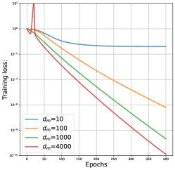
(b)

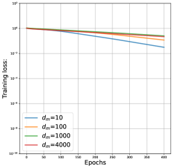
(c)

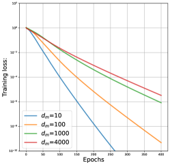
(d)

Figure 5: Comparison of convergence curve for different initialization schemes. The convergence speed under Lecun/He initialization is generally faster than that of NTK initialization with the same step size.

Appendix E Additional details on experiments

E.1 Additional result in Section 5.1

In this section, we present the convergence curve for different initialization schemes following the setup in Section 5.1. The results in Figures 5(a), 5(b) and 5(c) show that when using the same step size $\gamma=1$ for LeCun and He initialization exhibits similar behavior while NTK initialization leads to slower convergence. This is consistent with our theoretical finding. We also depict the result with larger step size $\gamma=10$ for NTK initialization in Figure 5(d), following our analysis in Section C.5.

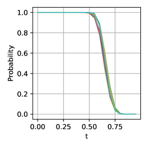
Figure 6: Verification of Assumption 3 on MNIST dataset.

E.2 Additional result and set-up in Section 5.2

We have validated Assumption 3 on language data in the main paper. Here we will validate it on image dataset. Specifically, we choose MNIST dataset and consider the embedding in the ViT as ${\bm{X}}$, then we plot $\mathbb{P}\left(\left|\left\langle{\bm{X}}_{n}^{\top}{\bm{X}}_{n},{\bm{X}}_{n^{\prime}}^{\top}{\bm{X}}_{n^{\prime}}\right\rangle\right|\geq t\right)$ as $t$ increases in Figure 6, where we could see exponential decay. The architecture of ViT is the same as in Section 5.2.

Additionally, in Figure 7, we can see that $d_{m}^{-1/2}$setting achieves faster convergence in training loss and higher test accuracy. In Figure 8, we conduct the experiment on MNIST with regression task by using the same architecture. We take two classes $\{0,1\}$ in MNIST for binary classification, the output of our regression is taken by $\text{sign}(f)$, and the training error is given by $\sum_{n=1}^{N}[\text{sign}(f({\bm{X}}_{n}))-y_{n}]^{2}$. We can see that the convergence speed of $d_{m}^{-1/2}$ is faster than that of $d_{m}^{-1}$. Overall, these separation results on both classification and regression tasks provide good justification for the $d_{m}^{-1/2}$ scaling.

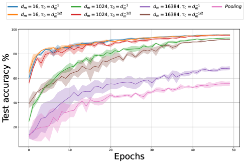
Figure 7: Test accuracy of classification task on MNIST dataset.

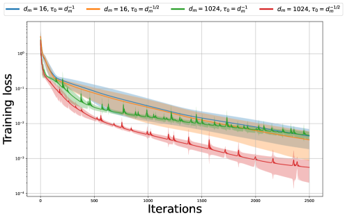
Figure 8: Regression task (with MSE loss) on MNIST dataset.

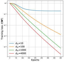
(a)

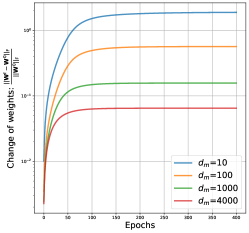
(b)

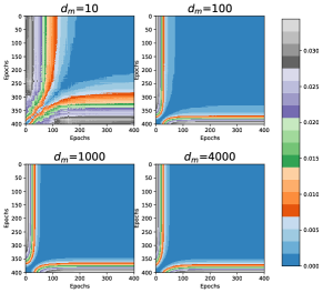
(c)

Figure 9: Experimental validation of the theoretical results on Transformers with $\tau_{0}=d_{m}^{-1}$ scaling trained on synthetic data. (a) Linear convergence. (b) Rate of change of the weights during training. Observe that the weights change very slowly after the $50^{\text{th}}$ epoch. (c) Evolution of the NTK during the training. The result mirrors the plot (b) and demonstrates how the kernel varies significantly at the beginning of the training and remains approximately constant later. As the width increases, the NTK becomes more stable.

Appendix F Limitation

Firstly, in this work, we prove the global convergence guarantee for Transformer under different initialization schemes. Nevertheless, we only consider the gradient descent training under squared loss. Our result does not cover SGD training and other loss functions, e.g., hinge loss and cross-entropy loss. Secondly, the model architecture being analyzed in this work is the encoder of Transformer which is widely used for regression problems or image classification problems. We do not consider the entire Transformer including the decoder, which is designed for sequence-to-sequence modeling. Lastly, our model does not cover the deep Transformer. We believe our analytic framework paves a way for further analyzing large-scale Transformer.

Appendix G Societal impact

This work offers a convergence analysis for the Transformer, which is a core element within contemporary large language models. Our theoretical analysis with realistic initializations and scaling schemes lays a theoretical foundation for the interested practitioner in the ML community to further study other priorities of Transformer such as generalization and in-context learning. We do not expect any negative societal bias from this work.

References

- Akyürek et al. (2023) Ekin Akyürek, Dale Schuurmans, Jacob Andreas, Tengyu Ma, and Denny Zhou. What learning algorithm is in-context learning? investigations with linear models. In International Conference on Learning Representations (ICLR), 2023.
- Alemohammad et al. (2021) Sina Alemohammad, Zichao Wang, Randall Balestriero, and Richard Baraniuk. The recurrent neural tangent kernel. In International Conference on Learning Representations (ICLR), 2021.
- Allen-Zhu et al. (2019a) Zeyuan Allen-Zhu, Yuanzhi Li, and Zhao Song. A convergence theory for deep learning via over-parameterization. In International Conference on Machine Learning (ICML), pages 242–252. PMLR, 2019a.
- Allen-Zhu et al. (2019b) Zeyuan Allen-Zhu, Yuanzhi Li, and Zhao Song. On the convergence rate of training recurrent neural networks. In Advances in neural information processing systems (NeurIPS), volume 32, 2019b.
- Arora et al. (2019a) Sanjeev Arora, Simon Du, Wei Hu, Zhiyuan Li, and Ruosong Wang. Fine-grained analysis of optimization and generalization for overparameterized two-layer neural networks. In International Conference on Machine Learning (ICML), 2019a.
- Arora et al. (2019b) Sanjeev Arora, Simon S Du, Wei Hu, Zhiyuan Li, Russ R Salakhutdinov, and Ruosong Wang. On exact computation with an infinitely wide neural net. Advances in neural information processing systems (NeurIPS), 32, 2019b.
- Bombari et al. (2022) Simone Bombari, Mohammad Hossein Amani, and Marco Mondelli. Memorization and optimization in deep neural networks with minimum over-parameterization. In Advances in neural information processing systems (NeurIPS), 2022.
- Brown et al. (2020) Tom Brown, Benjamin Mann, Nick Ryder, Melanie Subbiah, Jared D Kaplan, Prafulla Dhariwal, Arvind Neelakantan, Pranav Shyam, Girish Sastry, Amanda Askell, et al. Language models are few-shot learners. Advances in neural information processing systems (NeurIPS), 2020.
- Cao and Gu (2019) Yuan Cao and Quanquan Gu. Generalization bounds of stochastic gradient descent for wide and deep neural networks. In Advances in neural information processing systems (NeurIPS), 2019.
- Chen et al. (2022) Xiangning Chen, Cho-Jui Hsieh, and Boqing Gong. When vision transformers outperform resnets without pre-training or strong data augmentations. In International Conference on Learning Representations (ICLR), 2022.
- Chen et al. (2021) Zixiang Chen, Yuan Cao, Difan Zou, and Quanquan Gu. How much over-parameterization is sufficient to learn deep re{lu} networks? In International Conference on Learning Representations (ICLR), 2021.
- Chizat et al. (2019) Lenaic Chizat, Edouard Oyallon, and Francis Bach. On lazy training in differentiable programming. Advances in neural information processing systems (NeurIPS), 2019.
- Devlin et al. (2019) Jacob Devlin, Ming-Wei Chang, Kenton Lee, and Kristina Toutanova. BERT: Pre-training of deep bidirectional transformers for language understanding. In Proceedings of the 2019 Conference of the North American Chapter of the Association for Computational Linguistics: Human Language Technologies, Volume 1 (Long and Short Papers), pages 4171–4186, Minneapolis, Minnesota, June 2019. Association for Computational Linguistics. doi: 10.18653/v1/N19-1423.
- Dosovitskiy et al. (2021) Alexey Dosovitskiy, Lucas Beyer, Alexander Kolesnikov, Dirk Weissenborn, Xiaohua Zhai, Thomas Unterthiner, Mostafa Dehghani, Matthias Minderer, Georg Heigold, Sylvain Gelly, Jakob Uszkoreit, and Neil Houlsby. An image is worth 16x16 words: Transformers for image recognition at scale. In International Conference on Learning Representations (ICLR), 2021.
- Du et al. (2019a) Simon Du, Jason Lee, Haochuan Li, Liwei Wang, and Xiyu Zhai. Gradient descent finds global minima of deep neural networks. In International Conference on Machine Learning (ICML), 2019a.
- Du et al. (2019b) Simon S. Du, Xiyu Zhai, Barnabas Poczos, and Aarti Singh. Gradient descent provably optimizes over-parameterized neural networks. In International Conference on Learning Representations (ICLR), 2019b.
- Edelman et al. (2022) Benjamin L Edelman, Surbhi Goel, Sham Kakade, and Cyril Zhang. Inductive biases and variable creation in self-attention mechanisms. In International Conference on Machine Learning (ICML), pages 5793–5831, 2022.
- Fort et al. (2020) Stanislav Fort, Gintare Karolina Dziugaite, Mansheej Paul, Sepideh Kharaghani, Daniel M Roy, and Surya Ganguli. Deep learning versus kernel learning: an empirical study of loss landscape geometry and the time evolution of the neural tangent kernel. In Advances in neural information processing systems (NeurIPS), 2020.
- Gershgorin (1931) Semyon Aranovich Gershgorin. About delimiting the intrinsic values of a matrix. Proc. Russian Acad. Sci, page 749–754, 1931.
- Hastie et al. (2022) Trevor Hastie, Andrea Montanari, Saharon Rosset, and Ryan J Tibshirani. Surprises in high-dimensional ridgeless least squares interpolation. Annals of Statistics, 2022.
- Hron et al. (2020) Jiri Hron, Yasaman Bahri, Jascha Sohl-Dickstein, and Roman Novak. Infinite attention: Nngp and ntk for deep attention networks. In International Conference on Machine Learning (ICML), 2020.
- Huang et al. (2020) Kaixuan Huang, Yuqing Wang, Molei Tao, and Tuo Zhao. Why do deep residual networks generalize better than deep feedforward networks?—a neural tangent kernel perspective. Advances in neural information processing systems (NeurIPS), 33:2698–2709, 2020.
- Jacot et al. (2018) Arthur Jacot, Franck Gabriel, and Clement Hongler. Neural tangent kernel: Convergence and generalization in neural networks. In S. Bengio, H. Wallach, H. Larochelle, K. Grauman, N. Cesa-Bianchi, and R. Garnett, editors, Advances in neural information processing systems (NeurIPS), 2018.
- Jelassi et al. (2022) Samy Jelassi, Michael Eli Sander, and Yuanzhi Li. Vision transformers provably learn spatial structure. In Alice H. Oh, Alekh Agarwal, Danielle Belgrave, and Kyunghyun Cho, editors, Advances in neural information processing systems (NeurIPS), 2022.
- LeCun et al. (1998) Yann LeCun, Léon Bottou, Yoshua Bengio, Patrick Haffner, et al. Gradient-based learning applied to document recognition. Proceedings of the IEEE, 86(11):2278–2324, 1998.
- Lee et al. (2019) Jaehoon Lee, Lechao Xiao, Samuel Schoenholz, Yasaman Bahri, Roman Novak, Jascha Sohl-Dickstein, and Jeffrey Pennington. Wide neural networks of any depth evolve as linear models under gradient descent. Advances in neural information processing systems (NeurIPS), 2019.
- Li et al. (2023) Hongkang Li, Meng Wang, Sijia Liu, and Pin-Yu Chen. A theoretical understanding of shallow vision transformers: Learning, generalization, and sample complexity. In International Conference on Learning Representations (ICLR), 2023.
- Li and Liang (2018) Yuanzhi Li and Yingyu Liang. Learning overparameterized neural networks via stochastic gradient descent on structured data. Advances in neural information processing systems (NeurIPS), 2018.
- Liang and Rakhlin (2020) Tengyuan Liang and Alexander Rakhlin. Just interpolate: Kernel “ridgeless” regression can generalize. The Annals of Statistics, 2020.
- Liao and Couillet (2018) Zhenyu Liao and Romain Couillet. On the spectrum of random features maps of high dimensional data. In International Conference on Machine Learning, pages 3063–3071. PMLR, 2018.
- Liu et al. (2020) Chaoyue Liu, Libin Zhu, and Misha Belkin. On the linearity of large non-linear models: when and why the tangent kernel is constant. Advances in neural information processing systems (NeurIPS), 2020.
- Liu et al. (2022a) Chaoyue Liu, Libin Zhu, and Mikhail Belkin. Loss landscapes and optimization in over-parameterized non-linear systems and neural networks. Applied and Computational Harmonic Analysis, 2022a.
- Liu et al. (2021) Fanghui Liu, Zhenyu Liao, and Johan Suykens. Kernel regression in high dimensions: Refined analysis beyond double descent. In International Conference on Artificial Intelligence and Statistics (AISTATS), 2021.
- Liu et al. (2022b) Ze Liu, Han Hu, Yutong Lin, Zhuliang Yao, Zhenda Xie, Yixuan Wei, Jia Ning, Yue Cao, Zheng Zhang, Li Dong, et al. Swin transformer v2: Scaling up capacity and resolution. In Conference on Computer Vision and Pattern Recognition (CVPR), 2022b.
- Maas et al. (2011) Andrew L. Maas, Raymond E. Daly, Peter T. Pham, Dan Huang, Andrew Y. Ng, and Christopher Potts. Learning word vectors for sentiment analysis. In Proceedings of the 49th Annual Meeting of the Association for Computational Linguistics: Human Language Technologies, pages 142–150, Portland, Oregon, USA, June 2011. Association for Computational Linguistics.
- Mirsky (1975) Leon Mirsky. A trace inequality of john von neumann. Monatshefte für mathematik, 79:303–306, 1975.
- Montanari and Zhong (2022) Andrea Montanari and Yiqiao Zhong. The interpolation phase transition in neural networks: Memorization and generalization under lazy training. The Annals of Statistics, 50(5):2816–2847, 2022.
- Nguyen (2021) Quynh Nguyen. On the proof of global convergence of gradient descent for deep relu networks with linear widths. In International Conference on Machine Learning (ICML), 2021.
- Nguyen et al. (2021) Quynh Nguyen, Marco Mondelli, and Guido F Montufar. Tight bounds on the smallest eigenvalue of the neural tangent kernel for deep relu networks. In International Conference on Machine Learning (ICML), 2021.
- Nguyen and Mondelli (2020) Quynh N Nguyen and Marco Mondelli. Global convergence of deep networks with one wide layer followed by pyramidal topology. Advances in neural information processing systems (NeurIPS), 2020.