Total Variation Meets Differential Privacy

Abstract

The framework of approximate differential privacy is considered, and augmented by introducing the notion of “the total variation of a (privacy-preserving) mechanism” (denoted by $\eta$-TV). With this refinement, an exact composition result is derived, and shown to be significantly tighter than the optimal bounds for differential privacy (which do not consider the total variation). Furthermore, it is shown that $(\varepsilon,\delta)$-DP with $\eta$-TV is closed under subsampling. The induced total variation of commonly used mechanisms are computed. Moreover, the notion of total variation of a mechanism is extended to the local privacy setting and privacy-utility tradeoffs are investigated. In particular, total variation distance and KL divergence are considered as utility functions and upper bounds are derived. Finally, the results are compared and connected to the (purely) locally differentially private setting.

I Introduction

Given a database $D$ that contains private records (e.g., medical records), one would like to design a mechanism $M$ to answer queries issued by a curious (but not necessarily malicious) analyst (e.g., medical researchers). Such mechanism should provide useful answers while preserving the privacy of the individuals whose records are in $D$. In this context, differential privacy (DP) [1] was developed, and subsequently widely adopted, to quantify the privacy guarantees of a given mechanism $M$. Essentially, given any database $D$, any possible record, and the output $M(D)$ of a differentially-private $M$, the analyst cannot tell (except with insignificant probability) whether or not the record appears in $D$.

However, the analyst may issue several queries, thus degrading the privacy guarantees. Provable bounds on the resulting guarantees are referred to as composition theorems. Notably, pure differential privacy yields pessimistic composition theorems. As such, researchers have developed relaxations and variations of differential privacy to yield better composition behaviour, e.g., approximate DP [2], Rényi-DP [3], concentrated-DP [4], Gaussian DP [5], etc.

Herein, we focus on approximate DP and Gaussian DP as they have the clearest operational interpretation. In particular, Kairouz et al. [6] provided an equivalent characterization of $(\varepsilon,\delta)$-DP in terms of the achievable region of errors (type I and type II) of a binary hypothesis testing experiment. Utilizing this view, they proved an exact composition result for $(\varepsilon,\delta)$-DP in terms of a family of $\{(\varepsilon_{j},\delta_{j})\}_{j}$ parameters. As observed by Dong et al. [5], the binary hypothesis view also elucidates why composition results for $(\varepsilon,\delta)$-DP are pessimistic: the framework is not rich enough to capture the induced privacy region of the composed mechanisms (with one $(\varepsilon,\delta)$ pair). Instead, they parameterized the privacy guarantee by (the lower convex envelope of) the privacy region itself, and denoted it by $f$-DP [5]. Hence, they showed that $f$-DP is closed under composition, and proved an interesting limiting behavior wherein, under certain assumptions, the limit of the composition of $n$ $f$-DP mechanisms converges to the guarantees of the Gaussian mechanism.

We also study the privacy setting in which data remains private even from the statistician. Given distributions $P_{0}$ and $P_{1}$ and an $\varepsilon$-locally differentially private ($\varepsilon$-LDP) privatization mechanism $Q$, let $M_{0}$ and $M_{1}$ be the induced output marginals. Duchi et al. [7] proved bounds on the symmetrized KL divergence between $M_{0}$ and $M_{1}$ in the $\varepsilon$-LDP setting. Kairouz et al. [8] provided an $\varepsilon$-LDP binary mechanism that maximizes the total variation between $M_{0}$ and $M_{1}$ for all $P_{0}$ and $P_{1}$, and approximates the mechanism that maximizes the KL divergence between the marginals.

In this work, we introduce a simple refinement to (approximate) differential privacy to yield better composition results. Namely, we define the total variation (TV) of a mechanism, denoted by $\eta$-TV, so that we keep track of both the $(\varepsilon,\delta)$-parameters for DP and the $\eta$-parameter for TV. This retains an equivalent characterization in terms of binary hypothesis testing. Our contributions consist of the following:

• We prove an exact composition bound for $(\varepsilon,\delta)$-DP coupled with $\eta$-TV (Section III).

• We show the provided bounds can be significantly tighter than bounds where total variation is not taken into consideration (using examples, as well as asymptotic analysis [5]) (Sections III and IV).

• We show that $(\varepsilon,\delta)$-DP with $\eta$-TV is closed under subsampling (where the mechanism computes the query answer on a random subset of the database) (Section V).

• We compute the total variation of commonly used mechanisms and demonstrate an interesting connection with the staircase mechanism [9] (Section VI).

• We extend the notion of total variation of a mechanism to the local privacy setting and study privacy-utility tradeoffs (Section VII). In particular,

  • We refine and generalize existing bounds on the KL divergence between the output marginals of a privacy-preserving mechanism ([7], [8]).

  • We provide a mechanism that maximizes the total variation between the marginals in the case of $\varepsilon$-LDP with $\eta$-TV.

  • Finally, given an $\varepsilon$-LDP mechanism, we show how to construct and $\varepsilon$-LDP with $\eta$-TV mechanism, and use this result to connect the corresponding privacy-utility tradeoffs in the two settings (i.e., enforcing $\varepsilon$-LDP constraint versus enforcing $\varepsilon$-LDP and an $\eta$-TV constraint).

It is worth noting that total variation is arguably a “natural” measure to consider in privacy analysis and has been used in the literature as a privacy metric [10], and as a disparity metric [11], and indeed (as will be seen in this paper) it naturally appears in many existing analyses. Moreover, it is simple to compute bounds on total variation using, for instance, KL divergence or Chernoff information. As such, the computational overhead of keeping track of total variation (in order to get the above advantages) is relatively low.

II Preliminaries

Fix an alphabet $\mathcal{X}$ and an integer $m\in\mathbb{N}$. A database $D$ is an element in $\mathcal{X}^{m}$. Two databases that differ in one entry are called neighboring databases. A (query-answering) mechanism $M$ is a randomized map from $\mathcal{X}^{m}$ to an output space, which we denote by $\mathcal{Y}$.

Definition 1 (Differential Privacy (DP) [1])

Given $\varepsilon\geq 0$ and $\delta\in[0,1]$, a mechanism $M$ is $(\varepsilon,\delta)$-differentially private if, for all neighboring databases $D_{0}$ and $D_{1}$ and all $S\subseteq\mathcal{Y}$,

$${\rm\mathbf{Pr}}(M(D_{0})\in S)\leq e^{\varepsilon}{\rm\mathbf{Pr}}(M(D_{1})\in S)+\delta.$$

Wasserman and Zhou [12] and Kairouz et al. [6] provide an equivalent characterization of $(\varepsilon,0)$- and $(\varepsilon,\delta)$-DP, respectively, in terms of binary hypothesis testing. In particular, consider a mechanism $M$, two neighboring databases $D_{0}$ and $D_{1}$, and let $P_{0}$ and $P_{1}$ be the corresponding distributions over $\mathcal{Y}$ of $M(D_{0})$ and $M(D_{1})$. Given a random output $Y\in\mathcal{Y}$, an adversary aims to distinguish between

$H_{0}$: $Y\sim P_{0}$,  and  $H_{1}$: $Y\sim P_{1}$.

Let $h$ be any (possibly randomized) decision function, $h:\mathcal{Y}\rightarrow\{0,1\}$, and denote by $\beta_{\mathrm{I}}(P_{0},P_{1},h)=P_{0}(f(Y)=1)$ and $\beta_{\mathrm{I}\mathrm{I}}(P_{0},P_{1},h)=P_{1}(f(Y)=0)$ the type I and type II errors, respectively. Among such decision functions, the ROC curve (also called the tradeoff function [5]) describes the best type II error that can be achieved for a given level of type I error:

Definition 2 (ROC)

For a binary hypothesis testing experiment with distributions $P_{0}$ and $P_{1}$, the ROC curve, $f:[0,1]\to[0,1]$, is defined as

$$f(P_{0},P_{1})(t)=\inf_{h}\left\{\beta_{\mathrm{II}}(P_{0},P_{1},h):\beta_{\mathrm{I}}(P_{0},P_{1},h)\leq t\right\}.$$

Differential privacy can then be described in terms of constraints on ROC curves:

Theorem 1 ( [6, Theorem 2.1])

Given $\varepsilon\geq 0$ and $\delta\in[0,1]$, a mechanism $M$ is $(\varepsilon,\delta)$-DP if and only if for all neighboring databases $D_{0}$ and $D_{1}$ and all $t\in[0,1],$

$$t+e^{\varepsilon}f(P_{0},P_{1})(t)\geq 1-\delta,$$

$$e^{\varepsilon}t+f(P_{0},P_{1})(t)\geq 1-\delta,$$

where $M(D_{0})\sim P_{0}$ and $M(D_{1})\sim P_{1}$.

The region $(\beta_{\mathrm{I}},\beta_{\mathrm{II}})$ corresponding to the above constraints will also be referred to as the “privacy region” of the mechanism. The ROC curve corresponding to $(\varepsilon,\delta)$-DP is shown in Figure 1 (region in gray).

Figure 1: ROC corresponding to $(\varepsilon,\delta)$-DP.

In this work, we introduce “the total variation of the mechanism”. First, recall

Definition 3 (Total Variation)

Given two distributions $P$ and $Q$ over a common alphabet $\mathcal{Y}$, the total variation is defined as follows:

$$d_{TV}(P,Q)=\sup_{A\subseteq\mathcal{Y}}(P(A)-Q(A)).$$

Now, define

Definition 4 (Total Variation of a Mechanism)

Given $\eta\in[0,1]$, a mechanism $M$ has total variation less than $\eta$ (or $d_{TV}(M)\leq\eta$ or $\eta$-TV, for short) if, for all neighboring databases $D_{0}$ and $D_{1}$,

$$d_{TV}\left(P_{0},P_{1}\right)\leq\eta,$$ (1)

where $M(D_{0})\sim P_{0}$ and $M(D_{1})\sim P_{1}$.

Total variation is closely related to hypothesis testing: given two distributions $P$ and $Q$, then $d_{TV}(P,Q)\leq\eta$ if and only if $f(P,Q)(t)\geq 1-\eta-t$ for all $t\in[0,1]$.

Corollary 1

Given $\varepsilon\geq 0$, $\delta\in[0,1]$, and $\eta\in[0,\delta+(1-\delta)\frac{e^{\varepsilon}-1}{e^{\varepsilon}+1}]$, a mechanism $M$ is $(\varepsilon,\delta)$-DP and $\eta$-TV if and only if, for all neighboring databases $D_{0}$ and $D_{1}$ and all $t\in[0,1]$,

$$t+e^{\varepsilon}f(P_{0},P_{1})(t)\geq 1-\delta,$$ (2)

$$e^{\varepsilon}t+f(P_{0},P_{1})(t)\geq 1-\delta,$$ (3)

$$t+f(P_{0},P_{1})(t)\geq 1-\eta,$$ (4)

where $M(D_{0})\sim P_{0}$ and $M(D_{1})\sim P_{1}$.

As such, $M$ is $\eta$-TV can be rewritten as $(0,\eta)$-DP.

Remark 1

The maximum possible value for $\eta$ can be seen from the region in Figure 1, where $\beta_{\mathrm{I}}+\beta_{\mathrm{II}}\geq\frac{2(1-\delta)}{1+e^{\varepsilon}}=1-\left(\delta+(1-\delta)\frac{e^{\varepsilon}-1}{e^{\varepsilon}+1}\right)$.

The corresponding ROC curve is shown in Figure 2, with the privacy region shaded in gray.

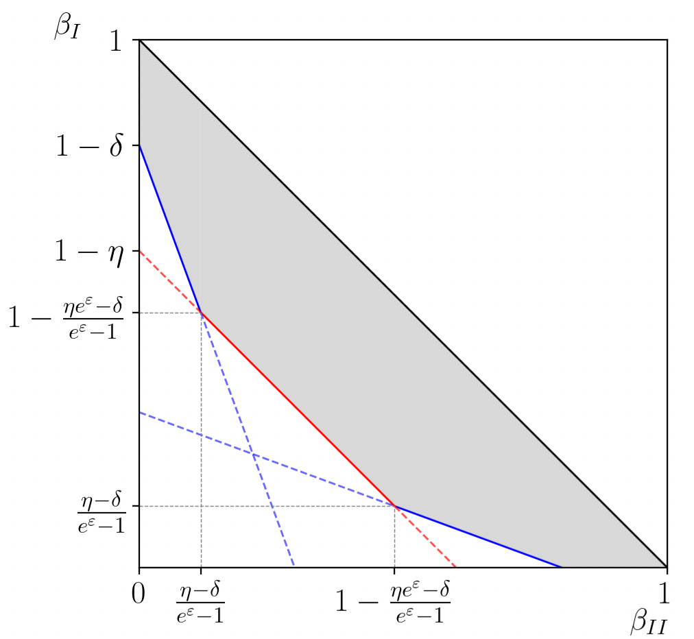
Figure 2: ROC corresponding to $(\varepsilon,\delta)$-DP $\eta$-TV.

III Main Result: Adaptive Composition

Our main result characterizes exactly the $k$-fold adaptive composition of $(\varepsilon,\delta)$-DP and $\eta$-TV mechanisms. More precisely, the $k$-fold binary hypothesis experiment is defined as follows:

• An adversary $\mathcal{A}$ chooses two neighboring databases $D_{0}$ and $D_{1}$.

• A parameter $b\in\{0,1\}$ is fixed (unknown to $\mathcal{A}$).

• $\mathcal{A}$ issues $k$ queries $q_{1}$, $q_{2},\ldots,q_{k}$, and receives $M_{1}(D_{b})$, $M_{2}(D_{b}),\ldots,M_{k}(D_{b})$. The choice of each query (or equivalently, the mechanism $M_{i}$) may depend on the outputs of previous queries.

• $\mathcal{A}$ guesses $\hat{b}\in\{0,1\}$.

Given that each $M_{i}$ is an $(\varepsilon,\delta)$-DP and $\eta$-TV mechanism, what is the privacy region induced by the above experiment?

Theorem 2

For any $\varepsilon\geq 0$, $\delta\in[0,1]$, and $\eta\in[\delta,\delta+\frac{(e^{\varepsilon}-1)(1-\delta)}{1+e^{\varepsilon}}]$, the class of $(\varepsilon,\delta)$-differentially private and $\eta$-total variation mechanisms satisfies

$$(j\varepsilon,1-(1-\delta)^{k}(1-\delta_{j}))\text{-differential privacy with }$$

$$d_{TV}=1-(1-\delta)^{k}(1-\delta_{0})$$

under $k$-fold adaptive composition, for all $j\in\{0,1,...,k\}$, where

$$\delta_{j}=\!\!\sum_{a=0}^{k-j-1}\!\!{k\choose a}\!\!\sum_{\ell=0}^{\lceil\frac{k-j-a}{2}\rceil-1} {k-a\choose\ell}\left(\frac{1-\alpha}{1+e^{\varepsilon}}\right)^{k-a}\alpha^{a}\left(e^{(k-\ell-a)\varepsilon}-e^{(\ell+j)\varepsilon}\right)$$ (5)

and $\displaystyle\alpha=1-\frac{(\eta-\delta)(1+e^{\varepsilon})}{(1-\delta)(e^{\varepsilon}-1)}$.

The proof follows the machinery developed by Kairouz et al. [6]. In particular, we introduce a “dominating” mechanism, i.e., a mechanism which exactly achieves the region described by the equations of Corollary 1. The achievability is then shown by analyzing the (non-adaptive) composition of the dominating mechanism (which admits a simple form). The key component of the converse, similarly to [6], is a result by Blackwell [13, Corollary of Theorem 10] which states the following: for two binary hypothesis testing experiments $A$ and $B$, if $f_{B}(t)\geq f_{A}(t)$ for all $t\in[0,1]$, then $B$ can be simulated from $A$. This is why the dominating mechanism yields the worst-case degradation (other mechanisms can be simulated from it).

III-A Comparison

The composition bound proved by Kairouz et al. [6] states that for any $\varepsilon$ and $\delta\in[0,1]$, the class of $(\varepsilon,\delta)$-differentially private mechanisms satisfies

$$(j\varepsilon,1-(1-\delta)^{k}(1-\delta_{j}))\text{-differential privacy}$$

under $k$-fold adaptive composition, for all $j\in\{k-2i:i=0,1,\ldots,\lfloor k/2\rfloor\}$, where

$$\delta_{j}=\frac{\sum_{\ell=0}^{\frac{k-j}{2}-1}{k\choose\ell}\left(e^{(k-\ell)\varepsilon}-e^{(\ell+j)\varepsilon}\right)}{(1+e^{\varepsilon})^{k}}.$$ (6)

Although the above bound is tight, commonly used mechanisms, like the Laplace mechanism, do not achieve the entire region described in Theorem 1. Taking into consideration the mechanism’s total variation leads to a better bound on the mechanism’s privacy region, as shown in Figure 3 (details of the computations can be found in section VI-A).

We illustrate the improved composition bound in Figure 4, with $\varepsilon=1$, $\delta=0$, and $\eta=0.7\frac{e^{\varepsilon}-1}{1+e^{\varepsilon}}$ (i.e., $\alpha=0.3$). Note that the refined composition bound involves lines with slopes of the form $-e^{\pm j\varepsilon}$ for $j\in\{0,1,...,k\}$, while the bound introduced in [6] only involves values of $j$ such that $0\leq j\leq k$ and $j$ and $k$ have the same parity. Even if one were to only observe the lines that correspond to values of $j$ that have the same parity as $k$ (blue vs green in Figure (4b)), the refined bound still improves on the previous bound.

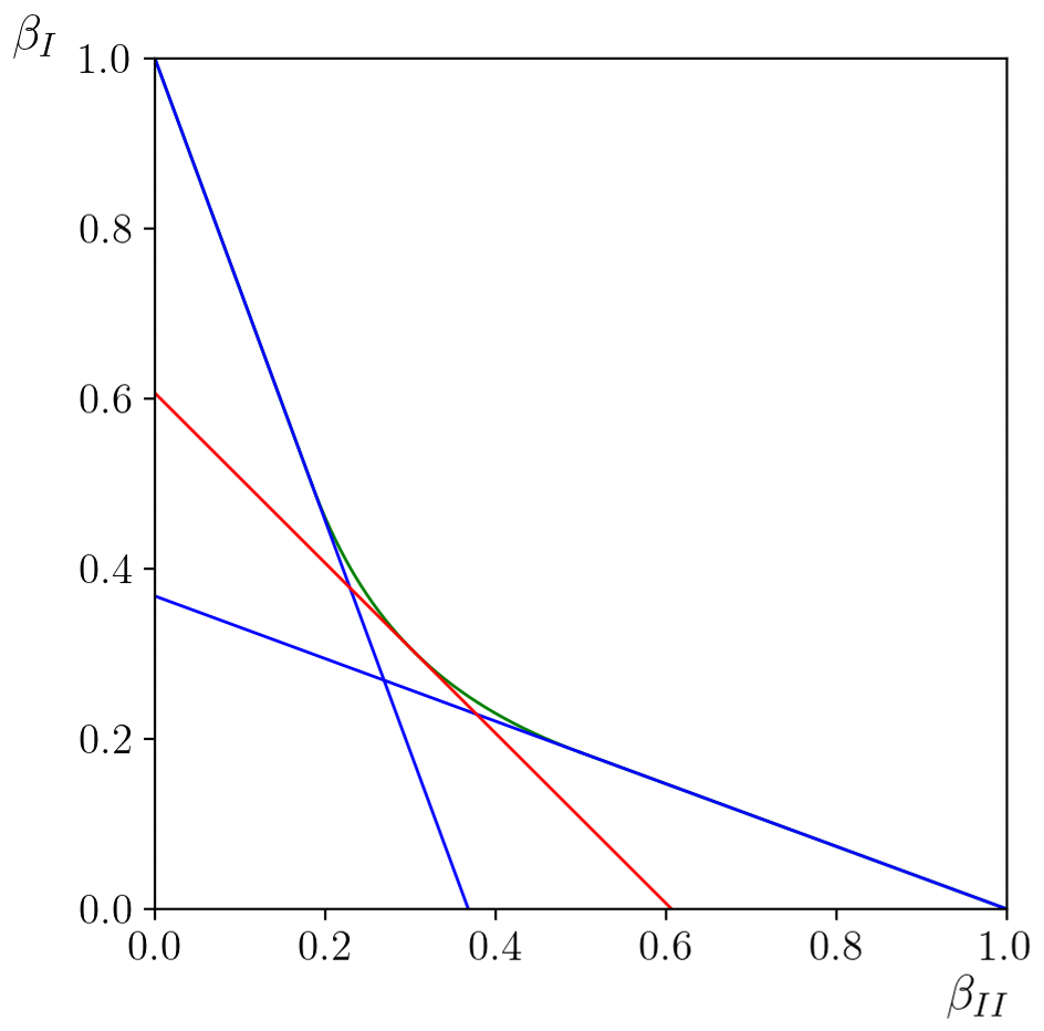
Figure 3: The Laplace mechanism’s exact tradeoff function is shown in green (for $\varepsilon=1$). The blue lines correspond to the differential privacy constraints. The red line corresponds to $\beta_{\mathrm{I}}=1-\eta_{\mathrm{Lap}}-\beta_{\mathrm{II}}$ where $\eta_{\mathrm{Lap}}=1-e^{-\varepsilon/2}$ is the total variation of the Laplace mechanism.

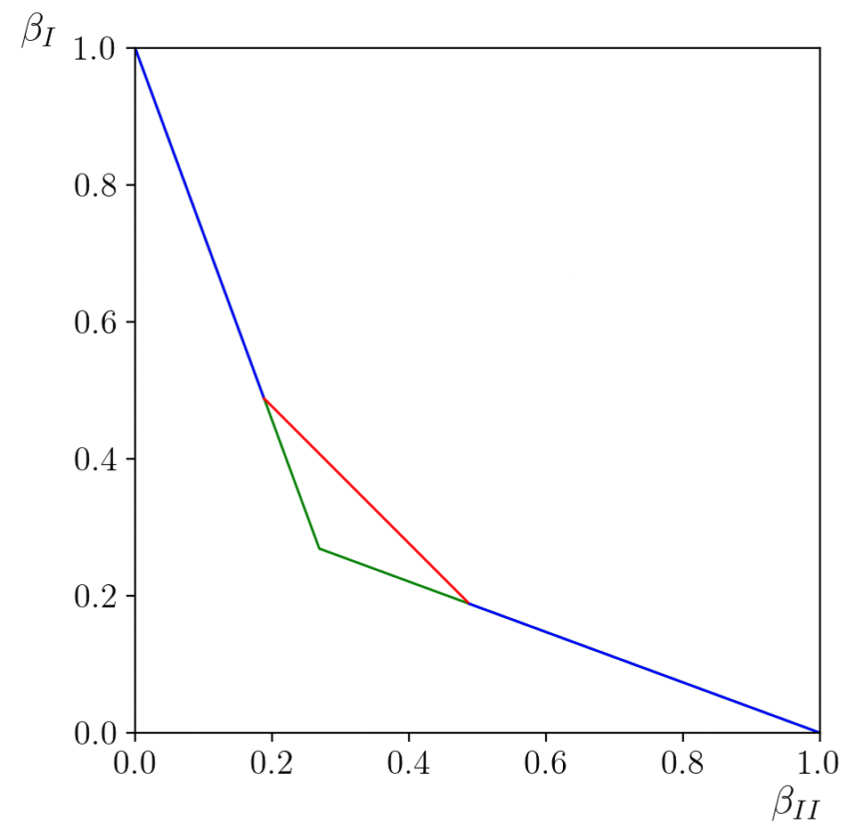
(a) The tradeoff functions for $k=1$.

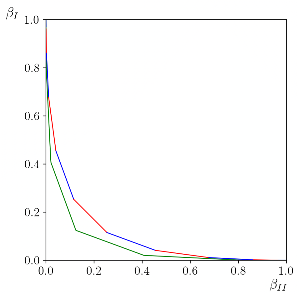
(b) The tradeoff functions for k=5

Figure 4: Dominating mechanisms for $\varepsilon=1$, $\delta=0$, and $\alpha=0.3$. The green line shows the tradeoff function of $\varepsilon$-DP (given by equation (6)). The blue and red lines plot the tradeoff given by Theorem 2, where they correspond, respectively, to odd (same parity as $k=5$) and even choices of $j$ in equation (5).

III-B Proof

III-B1 Dominating Mechanism

Kairouz [6] et al. introduced a mechanism, which we will denote by $M_{\varepsilon,\delta}:\mathcal{X}^{m}\to\{0,1\}$, that dominates all $(\varepsilon,\delta)$-differentially private mechanisms in the following sense: for any $(\varepsilon,\delta)$-DP mechanism $M:\mathcal{X}^{m}\to\mathcal{Y}$, for any pair of databases $D_{0}$ and $D_{1}$, there exists a (possibly randomized) mapping $T:\{0,1\}\to\mathcal{Y}$ such that, $M(D)$ and $T(M_{\varepsilon,\delta}(D))$ have the same distribution, where $D\in\{D_{0},D_{1}\}$. We adopt a similar approach, and provide a mechanism that dominates all $(\varepsilon,\delta)$-differentially private mechanisms with total variation $\eta$. Due to lack of space, we provide herein the proof of the case $\delta=0$ only.

The following mechanism (as in [6]) does not depend on the database entries or the query; it only depends on the hypothesis, and will be denoted by $M_{\varepsilon,0,\eta}$. It outputs $X_{0}\sim P_{0}$ in the case of the null hypothesis, and $X_{1}\sim P_{1}$ in the case of the alternative hypothesis, where $P_{0}$ and $P_{1}$ are defined as follows, for $\varepsilon\geq 0$ and $\alpha\in[0,1]$:

$$P_{0}=\begin{cases}\frac{(1-\alpha)e^{\varepsilon}}{(1+e^{\varepsilon})},&\text{for }x=0,\\ \alpha,&\text{for }x=1,\\ \frac{(1-\alpha)}{(1+e^{\varepsilon})},&\text{for }x=2,\end{cases}$$ (7)

and

$$P_{1}=\begin{cases}\frac{(1-\alpha)}{(1+e^{\varepsilon})},&\text{for }x=0,\\ \alpha,&\text{for }x=1,\\ \frac{(1-\alpha)e^{\varepsilon}}{(1+e^{\varepsilon})},&\text{for }x=2.\end{cases}$$ (8)

The above mechanism’s total variation is $d_{TV}(P_{0},P_{1})=\frac{(e^{\varepsilon}-1)(1-\alpha)}{(1+e^{\varepsilon})}$. So for a target $\eta\in[0,\frac{e^{\varepsilon}-1}{e^{\varepsilon}+1}]$, we set $\alpha=1-\eta\frac{e^{\varepsilon}+1}{e^{\varepsilon}-1}$. For $\eta=\frac{e^{\varepsilon}-1}{e^{\varepsilon}+1}$, we recover $M_{\varepsilon,0}$. It is easy to verify that $f(P_{0},P_{1})$ exactly achieves the region described in Corollary 1.

III-B2 Composed Dominating Mechanism

We show that the region described in Theorem 2 is achievable by analyzing the non-adaptive composition of $M_{\varepsilon,0,\eta}$, i.e., in the $k$-fold binary hypothesis experiment, we set $M_{i}=M_{\varepsilon,0,\delta}$ for all $i=1,2,\ldots,k$.

Since the privacy region of the composed mechanism is a convex set, we can describe its boundaries with a set of lines tangent to its envelope. For a slope $-\gamma$, we want to find the largest shift $1-\delta^{\prime}$ such that the line $\beta_{\mathrm{I}}=-\gamma\beta_{\mathrm{II}}+1-\delta^{\prime}$ is below the tradeoff curve.

For some acceptance set $A$, consider the point $(\beta_{\mathrm{II}}(A),\beta_{\mathrm{I}}(A))$ included in the composed mechanism’s privacy region. We want $-\gamma\beta_{\mathrm{II}}(A)+1-\delta^{\prime}\leq\beta_{\mathrm{I}}(A)$, i.e.,

$$\delta^{\prime} \geq 1-\beta_{\mathrm{I}}(A)-\gamma\beta_{\mathrm{II}}(A)$$ (9)

$$=P_{0}(A)-\gamma P_{1}(A).$$ (10)

We choose the smallest $\delta^{\prime}$ such that the inequality (9) is satisfied for all $A$, i.e.,

$$\delta^{\prime}=\max_{\begin{subarray}{c}A\in\mathcal{X}\end{subarray}}\{P_{0}(A)-\gamma P_{1}(A)\}.$$

We represent the output of a $k$-fold composition experiment as a sequence $s^{k}\in\{0,1,2\}^{k}$, and use the following notations:

$$a=|\{i:s_{i}^{k}=1\}|,\text{ and }\ell=|\{i:s_{i}^{k}=2\}|.$$ (11)

Let $\tilde{P_{0}}$ be the probability of obtaining a specific sequence $s^{k}$ when the true database is $D_{0}$ and $\tilde{P_{1}}$ the probability of obtaining $s^{k}$ when the true database is $D_{1}$ under $k$-fold composition. Since the outputs of the mechanisms are i.i.d.,

$$\tilde{P_{0}}(s^{k}) =P_{0}(X=0)^{k-\ell-a}P_{0}(X=1)^{a}P_{0}(X=2)^{\ell}$$

$$=\left(\frac{1-\alpha}{1+e^{\varepsilon}}\right)^{k-a}e^{(k-\ell-a)\varepsilon}\alpha^{a},$$

and

$$\tilde{P_{1}}(s^{k}) =P_{1}(X=0)^{k-\ell-a}P_{1}(X=1)^{a}P_{1}(X=2)^{\ell}$$

$$={\left(\frac{1-\alpha}{1+e^{\varepsilon}}\right)}^{k-a}e^{\ell\varepsilon}\alpha^{a}.$$

By the Neyman-Pearson lemma [14, Theorem 11.7.1], points on the ROC curve are achieved by tests of the form $\{s^{k}:\frac{\tilde{P}_{0}(s^{k})}{P_{1}(s^{k})}>T\}$, for some threshold $T$. Letting

$$E\equiv\{0\leq\tilde{\varepsilon}\leq\infty:\tilde{P_{0}}(s_{k})=e^{\tilde{\varepsilon}}\tilde{P_{1}}(s_{k})\text{ for some }x\in\mathcal{X}\},$$

any $\tilde{\varepsilon}\notin E$ does not contribute to the boundary of the privacy region.

Remark 2

It is sufficient to consider $\tilde{\varepsilon}\geq 0$ as the tradeoff function is symmetric due to the symmetry of $P_{0}$ and $P_{1}$. The symmetry is then accounted for by the symmetry of $(\varepsilon,\delta)$-DP.

Noting that

$$\frac{\tilde{P_{0}}(s_{k})}{\tilde{P_{1}}(s_{k})}=\frac{e^{(k-\ell-a)\varepsilon}}{e^{\ell\varepsilon}},\text{ it follows }\tilde{\varepsilon}=(k-2\ell-a)\varepsilon.$$

Therefore, the distinct values that $\tilde{\varepsilon}$ can take are of the form $\varepsilon_{j}=j\varepsilon$ where $j\in\{0,1,...,k\}$. To every $\varepsilon_{j}$ corresponds a $\delta_{j}$ of the form

$$\delta_{j}=\max_{\begin{subarray}{c}A\in\mathcal{X}^{k}\end{subarray}}\{\tilde{P_{0}}(A)-e^{\varepsilon_{j}}\tilde{P_{1}}(A)\},$$

where $A$ is the acceptance region. For a fixed $j$, we consider the sequences $s_{k}$ such that $\tilde{P_{0}}(s_{k})-e^{j\varepsilon}\tilde{P_{1}}(s_{k})>0$, i.e.

$${\left(\frac{1-\alpha}{1+e^{\varepsilon}}\right)}^{k-a}\alpha^{a}\left(e^{(k-\ell-a)\varepsilon}-e^{(\ell+j)\varepsilon}\right) >0.$$

There are ${k\choose a}{k-a\choose\ell}$ sequences of the form described in (11), but we are only interested in the sequences that satisfy $e^{(k-\ell-a)\varepsilon}-e^{(\ell+j)\varepsilon}>0$, or $k-j>2\ell+a$, hence the summation bounds in equation (5).

III-B3 Converse

Since the tradeoff function of $M_{\varepsilon,0,\eta}$, $f_{{\varepsilon,0,\eta}}$, matches with equality the constraints given in Corollary 1, the tradeoff function of any $\varepsilon$-DP and $\eta$-TV mechanism $M$ must satisfy $f_{M}(t)\geq f_{{\varepsilon,0,\eta}}(t)$ for all $t\in[0,1]$. Hence by Blackwell’s result [13, Corollary of Theorem 10], $M$ can be simulated from $M_{\varepsilon,0,\delta}$. Given this fact, one can follow exactly the converse proof in [6] to show that the output of the $k$-fold composition of any $\varepsilon$-DP and $\eta$-TV mechanisms can also be simulated using the (non-adaptive) $k$-fold composition of $M_{\varepsilon,0,\eta}$, hence the corresponding tradeoff function will be greater than the composition of $M_{\varepsilon,0,\eta}$.

IV Asymptotic Behaviour

Inspired by the hypothesis testing view of differential privacy [6, 12], Dong et al. [5] introduced a new privacy measure, called $f$-differential privacy, based directly on tradeoff functions (i.e., ROC curves):

Definition 5 ($f$-DP [5])

Let $f:[0,1]\to[0,1]$ be a convex, continuous, non-increasing function, satisfying $f(x)\leq 1-x$. A mechanism $M$ is $f$-DP if for all neighboring databases $D_{0}$ and $D_{1}$ and $t\in[0,1]$,

$$f(P_{0},P_{1})(t)\geq f(t),$$ (12)

where $M(D_{0})\sim P_{1}$ and $M(D_{1})\sim P_{1}$.

As such, $(\varepsilon,\delta)$-DP, as well as $(\varepsilon,\delta)$-DP with $\eta$-TV, are special cases of $f$-DP, with $f$ given by the corresponding curves shown in Figure 2.

Notably, the composition of $f$-DP mechanisms is also $f$-DP (with a potentially different $f$), i.e., $f$-DP is closed under composition. Moreover, the authors [5] show that composition for $f$-DP follows a central limit theorem-like behavior in the following sense. Given $\mu\in\mathbb{R}$, let

$$G_{\mu}(\alpha)=f(\mathcal{N}(0,1),\mathcal{N}(\mu,1))(\alpha),$$ (13)

for $\alpha\in[0,1]$. Then, the composition of $n$ $f$-DP mechanisms can be approximated by $G_{\mu}$ (with an appropriate $\mu$) [5, Theorem 3.4]. Indeed, under suitable assumptions, the limit of the composition is equal to $G_{\mu}$ [5, Theorem 3.5]. For instance, letting $\varepsilon_{n}=\frac{\mu}{\sqrt{n}}$, then the composition of $n$ $\varepsilon_{n}$-DP mechanisms converges to $G_{\mu}$ [5, Theorem 3.6]. Here, we provide an analogous result for $\varepsilon$-DP with $\eta$-TV (proof deferred to Appendix -E):

Theorem 3

Consider a triangular array $\{(\varepsilon_{ni},\eta_{ni}):1\leq i\leq n\}_{n=1}^{\infty}$ such that $\displaystyle\lim_{n\rightarrow\infty}\sum_{i=1}^{n}\varepsilon_{ni}\eta_{ni}=\frac{\mu^{2}}{2}$ for some $\mu\geq 0$, and $\displaystyle\lim_{n\rightarrow\infty}\max_{1\leq i\leq n}\varepsilon_{ni}=0$. Let $M_{ni}:\mathcal{X}^{m}\to\mathcal{Y}_{ni}$ be an $\varepsilon_{ni}$-DP and $\eta_{ni}$-TV mechanism, and let $M_{n}(D)=(M_{n1}(D),\ldots,M_{nn}(D))$, $D\in\mathcal{X}^{m}$. Then, there exists a sequence of functions $\{f_{n}\}$ such that $M_{n}(D)$ is $f_{n}$-DP and

$$\lim_{n\rightarrow\infty}f_{n}=G_{\mu},$$ (14)

uniformly over $[0,1]$, where $G_{\mu}$ is defined in Eq. (13).

For pure differential privacy, $\eta=\frac{e^{\varepsilon}-1}{e^{\varepsilon}+1}\approx\frac{\varepsilon}{2}$ for small $\varepsilon$, so that the above result matches Theorem 3.6 of [5]. However, if for small $\varepsilon$, $\eta\approx\frac{\varepsilon}{c_{0}}$ for some $c_{0}>2$, then: if Theorem 3.6 of [5] yields a parameter $\mu$, Theorem 3 will yield $\mu\sqrt{\frac{2}{c_{0}}}$. It is worth noting that one can always reduce the total variation of a mechanism by a factor $(1-\delta^{\prime})$ by passing its output through an erasure channel with parameter $\delta^{\prime}$. Moreover, let $c_{1}\in(0,1/2)$, $\varepsilon_{ni}=\frac{\mu}{n^{c_{1}}}$, and $\eta_{ni}=\frac{\mu}{2n^{1-c_{1}}}$, for all $1\leq i\leq n$. Then, the conditions of the theorem are satisfied, and the limit of the composition is $G_{\mu}$. As opposed to decaying as $1/\sqrt{n}$, $\varepsilon_{n}$ could decay with an arbitrarily small power of $n$, as long as this is “compensated” for with a faster decay for the total variation. Finally, it is worth noting that, as compared to the $f$-DP framework, $(\varepsilon,\delta)$-DP with $\eta$-TV is significantly simpler as we keep track of only three parameters, while still yielding considerable advantages over $(\varepsilon,\delta)$-DP. Moreover, it is easier to work with from a design perspective (choosing $\varepsilon$ and $\eta$ parameters versus choosing a function).

Remark 3

Although Theorem 3 was stated for non-adaptive composition, one could allow adaptive choices of $M_{ni}$ and retain the same result (this is due to a tightness result by Dong et al. [5, Theorem 3.2]).

V Subsampling

Subsampling is a simple method to “amplify” privacy guarantees: before answering a query on a given database of size $n$, first choose uniformly at random a subset of size $m$, $1\leq m\leq n$. This procedure will be denoted by $\mathrm{Sample}_{m}$. Then, compute the query answer on the sampled database.

Proposition 1

Given $\varepsilon>0$, $\delta\in[0,1]$, and $\eta\in[0,1]$, if $M:\mathcal{X}^{m}\to\mathcal{Y}$ is ($\varepsilon$,$\delta$)-DP and $\eta$-TV, then the subsampled mechanism $M\circ\mathrm{Sample}_{m}:\mathcal{X}^{n}\to\mathcal{Y}$ is $p\eta$-TV and ($\log\left(1+p\left(e^{\varepsilon}-1\right)\right),p\delta$)-DP on $\mathcal{X}^{n}$, where $m\leq n$ and $p=\frac{m}{n}$.

The proof (deferred to Appendix -F) is based on the privacy amplification by subsampling result for ($\varepsilon$,$\delta$)-DP appearing in [15, 16, 17] and stated in  [18, Theorem 29], hence its tightness derives from the tightness of the $(\varepsilon,\delta)$-DP result. As such, $(\varepsilon,\delta)$-DP with $\eta$-TV is closed under subsampling. Moreover, as can be seen from the proof, it holds in general that if $M$ is $\eta$-TV, then $M\circ\mathrm{Sample}_{m}$ is $p\eta$-TV.

VI Applications

In this section, we compute the total variation for the Laplace, Gaussian, and staircase mechanisms, to demonstrate improvement and/or simplicity of analysis for commonly used mechanisms. Using well-known bounds on the total variation (e.g., Pinsker’s inequality), one could also derive simple closed-form bounds on the total variation of the composition. While one could efficiently approximate the composed tradeoff functions of mechanisms using Fourier-based methods [19, 20, 21], doing so requires the CDF of the “privacy loss” random variable and may not lead to a closed form. We also discuss an additional use-case for keeping track of the total variation of a mechanism in the context of Membership Inference Attacks.

VI-A Laplace Mechanism

The probability density function of a Laplace distribution centered at $0$ and with scale $b$ is

$$Lap(x|b)=\frac{1}{2b}\exp(-\frac{|x|}{b}),$$ (15)

and will be denoted by $Lap(b)$. For a (query) function $q:\mathcal{X}^{m}\rightarrow\mathbb{R}$, the output of the Laplace mechanism, denoted $M_{\mathrm{Lap}}$, is $M_{\mathrm{Lap}}(X)=q(X)+Y$ where $Y\sim Lap(\Delta/\varepsilon)$, and the query sensitivity $\Delta$ is defined as

$$\Delta=\max_{\begin{subarray}{c}D\text{ and }D^{\prime}\text{ neighbours}\end{subarray}}|q(D)-q(D^{\prime})|.$$ (16)

$M_{\mathrm{Lap}}$ is $\varepsilon$-DP and $d_{TV}(M_{\mathrm{Lap}})=1-e^{-\frac{\varepsilon}{2}}$ (derivation in Appendix -G).

VI-B Gaussian Mechanism

The total variation of a Gaussian mechanism operating on a statistic $\theta$ with variance $\sigma^{2}=\frac{sens(\theta)^{2}}{\mu^{2}}$ for $\mu\geq 0$ is

$$d_{TV} =2\Phi\Bigl{(}\frac{\mu}{2}\Bigr{)}-1,$$ (17)

where $\Phi$ is the Standard Normal CDF (derivation in Appendix -H).

VI-C Staircase Mechanism

Geng et al. [22] studied privacy-utility tradeoffs using differential privacy. They demonstrated that, for a large family of utility functions, the optimal noise-adding mechanism is the “staircase mechanism”. That is, the noise is drawn from a staircase-shaped probability distribution with probability density function

$$f_{\gamma}(x)=\left\{\begin{aligned} &a(\gamma),&&x\in[0,\gamma\Delta),\\ &e^{-\varepsilon}a(\gamma),&&x\in[\gamma\Delta,\Delta),\\ &e^{-k\varepsilon}f_{\gamma}(x-k\Delta),&&[k\Delta,(k+1)\Delta),~{}k\in\mathbb{N},\\ &f_{\gamma}(-x),&&x<0.\end{aligned}\right.$$

where $\displaystyle a(\gamma)=\frac{1-e^{-\varepsilon}}{2\Delta(\gamma+e^{-\varepsilon}(1-\gamma))}$, $\gamma\in\mathbb{R}^{+}$. The total variation of the staircase mechanism is given by (derivation in Appendix -I1):

$$d_{TV}\!\!=\!\!\left\{\begin{aligned} &\frac{(1-e^{-\varepsilon})(2\gamma(1-e^{-\varepsilon})+e^{-\varepsilon})}{2(\gamma+e^{-\varepsilon}(1-\gamma))},&\gamma\in[0,\frac{1}{2}),\\ &\frac{1-e^{-\varepsilon}}{2(\gamma+e^{-\varepsilon}(1-\gamma))},&\gamma\in[\frac{1}{2},\infty).\end{aligned}\right.$$

Remarkably, the staircase mechanism with total variation $\eta$ achieves exactly the privacy region corresponding to $(\varepsilon,0)$-DP and $\eta$-TV (proof in Appendix -I2).

For $\gamma=\frac{1}{2}$, $d_{TV}=\frac{e^{\varepsilon}-1}{e^{\varepsilon}+1}$, which corresponds to the total variation of the $(\varepsilon,0)$-differentially private dominating mechanism introduced by Kairouz et al. [6], or to that of the mechanism that we introduced in Section III-B for $\alpha=0$. For $\gamma=0.0139$, $\alpha\approx 0.3$, the corresponding tradeoff function consists of the blue and red lines in Figure 4a, and therefore the composition exactly corresponds to the blue and red lines in Figure 4b.

VI-D Membership Inference Attacks

Another motivation for keeping track of a mechanism’s total variation is in the context of Membership Inference Attacks (MIAs), in which the attacker tries to determine whether a given record was part of the model’s training data. Kulynych et al. [11] studied the phenomenon of disparate vulnerability to MIAs, i.e., the unequal success rate of MIAs against different population subgroups (or the difference between subgroup vulnerability to MIAs). They showed that the worst-case vulnerability of a subgroup to MIAs is bounded by the total variation of the mechanism, and consequently, so is the disparity. It is therefore useful to keep track of the total variation of a mechanism under composition to obtain guarantees against MIAs. We know from our refined composition result that a bound on the total variation under $k$-fold composition is $d_{TV}=1-(1-\delta)^{k}(1-\delta_{0})$ (and that it is exact when the mechanism is dominating, e.g., staircase mechanism). We also know that a mechanism that is $\mu$-GDP, is $\sqrt{k}\mu$-GDP under $k$-fold composition ([5]); therefore, in the case of the Gaussian mechanism, the total variation under $k$-fold composition is exactly $2\Phi\bigl{(}\frac{\sqrt{k}\mu}{2}\bigr{)}-1$.

VII Total Variation with Local Differential Privacy

We extend the notion of total variation of a mechanism to the local privacy setting. Consider a setting where $n$ data providers each owning a data $X_{i}\in\mathcal{X}$, each independently sampled from some distribution $P_{\nu}$. A statistical privatization mechanism $Q$ is a conditional distribution that maps $X_{i}\in\mathcal{X}$ stochastically to $Y_{i}\in\mathcal{Y}$, privatized views of $X_{i}$’s. The mechanism is used locally by all individuals. In this section, we assume all alphabets are finite.

Definition 6 (Local Differential Privacy)

For $\varepsilon\geq 0$, a mechanism $Q$ is $\varepsilon$-locally differentially private if

$$\sup_{S\subset\mathcal{Y},x,x^{\prime}\in\mathcal{X}}\frac{Q(S|x)}{Q(S|x^{\prime})}\leq e^{\varepsilon}.$$ (18)

We define the total variation of a mechanism in the context of local privacy:

Definition 7

Given $\eta\in[0,1]$, a mechanism $Q_{Y|X}$ is said to be $\eta$-TV locally (or $d_{TV}(Q)\leq\eta$ for short) if

$$\max_{x,x^{\prime}}\,d_{TV}\bigl{(}Q(.|X=x),Q(.|X=x^{\prime})\bigr{)}=\eta.$$ (19)

In other words, the Dobrushin coefficient [23] of $Q$, typically denoted by $\eta_{TV}(Q)$, is given by $\eta$, i.e., $\eta_{TV}(Q)=\eta$. The connection to contraction coefficients is reminiscent of the recent results on the connection between local differential privacy and the contract coefficients for $E_{\gamma}$ divergences [24, 25].

We first show an upper bound on $d_{TV}(Q)$ for locally differentially private mechanisms (proof deferred to Appendix -J):

Proposition 2

Given $\varepsilon\geq 0$, if a mechanism $Q_{Y|X}$ is $\varepsilon$-locally differentially private, then

$$d_{TV}(Q)\leq\frac{e^{\varepsilon}-1}{e^{\varepsilon}+1}.$$ (20)

With the refined privacy notion in hand, we can now study privacy-utility tradeoffs. In particular, we are interested in utility functions that are relevant for hypothesis testing or more general statistical analyses, such as $f$-divergences. To that end, consider the following problem. Given two distributions $P_{0}$ and $P_{1}$ on $\mathcal{X}$,

$$\underset{Q_{Y|X}}{\text{maximize }} ~{}D_{f}(M_{0}||M_{1})$$

subject to $$~{}Q_{Y|X}\text{ is }\varepsilon\text{-LDP},$$

$$~{}d_{TV}(Q_{Y|X})\leq\eta,$$

where $D_{f}$ is an $f$-divergence, and $M_{0}$ and $M_{1}$ are the induced marginals by $P_{0}$ and $P_{1}$, respectively. That is, for $S\in\mathcal{Y}$ and $\nu\in\{0,1\}$,

$$M_{\nu}(S)\equiv\sum_{x\in\mathcal{X}}Q(S|x)P_{\nu}(x).$$ (21)

In the following, we consider the above optimization problem for total variation, and for symmetrized KL divergence. Finally, we relate the optimal values of the optimzation problems with and without the $\eta$-TV constraint.

VII-A Total Variation Bound

In this section, we consider $D_{f}$ to be the total variation, i.e., we would like to maximize the total variation between the marignals, $d_{TV}(M_{0}||M_{1})$. This problem was considered by Kairouz et al. [8] for the case of $\varepsilon$-locally DP mechanisms. They exactly characterized the solution as follows:

Theorem 4 ([8, Theorem 6, Corollary 11])

Given $\varepsilon\geq 0$, if $Q$ is $\varepsilon$-LDP, then

$$\|M_{0}-M_{1}\|_{TV}\leq\frac{e^{\varepsilon}-1}{e^{\varepsilon}+1}\|P_{0}-P_{1}\|_{TV}.$$ (22)

Moreover, equality is achieved by the binary mechanism defined by

$$Q^{\star}_{b}(0|x)=\begin{cases}\frac{e^{\varepsilon}}{1+e^{\varepsilon}}&\text{if }P_{0}(x)\geq P_{1}(x),\\ \frac{1}{1+e^{\varepsilon}}&\text{if }P_{0}(x)<P_{1}(x),\end{cases}$$ (23)

and

$$Q^{\star}_{b}(1|x)=\begin{cases}\frac{e^{\varepsilon}}{1+e^{\varepsilon}}&\text{if }P_{0}(x)<P_{1}(x),\\ \frac{1}{1+e^{\varepsilon}}&\text{if }P_{0}(x)\geq P_{1}(x).\end{cases}$$ (24)

We generalize the above theorem to include the $\eta$-TV constraint:

Theorem 5

Given $\varepsilon\geq 0$ and $\eta\in[0,\frac{e^{\varepsilon}-1}{e^{\varepsilon}+1}]$, if $Q$ is $\varepsilon$-LDP and $\eta$-TV, then

$$\|M_{0}-M_{1}\|_{TV}\leq\eta\|P_{0},P_{1}\|_{TV}.$$ (25)

Moreover, equality is achieved by the binary mechanism with erasure defined by

$$Q^{\star}(0|x) =\begin{cases}(1-\alpha)\frac{e^{\varepsilon}}{1+e^{\varepsilon}}&\text{if }P_{0}(x)\geq P_{1}(x),\\ (1-\alpha)\frac{1}{1+e^{\varepsilon}}&\text{if }P_{0}(x)<P_{1}(x),\end{cases}$$ (26)

$$Q^{\star}(1|x) =\begin{cases}(1-\alpha)\frac{e^{\varepsilon}}{1+e^{\varepsilon}}&\text{if }P_{0}(x)<P_{1}(x),\\ (1-\alpha)\frac{1}{1+e^{\varepsilon}}&\text{if }P_{0}(x)\geq P_{1}(x),\end{cases}$$ (27)

$$Q^{\star}(e|x) =\alpha,$$ (28)

where $\alpha=1-\eta\frac{e^{\varepsilon}+1}{e^{\varepsilon}-1}$.

Remark 4

By Proposition 2, $\eta(Q)\leq\frac{e^{\varepsilon}-1}{e^{\varepsilon}+1}$ if $Q$ is $\varepsilon$-LDP. Hence, the inequality in Theorem 4 follows from Theorem 5 and Proposition 2. Moreover, the equality in Theorem 4 follows by choosing $\eta=\frac{e^{\varepsilon}-1}{e^{\varepsilon}+1}$ in Theorem 5.

Proof:

Recall Dobrushin’s classical result [23]:

$$\sup_{\begin{subarray}{c}P_{0},P_{1}\\ P_{0}\neq P_{1}\end{subarray}}\frac{||M_{0}-M_{1}||_{\text{TV}}}{||P_{0}-P_{1}||_{\text{TV}}}=\sup_{x,x^{\prime}}\,d_{TV}\bigl{(}Q(.|X=x),Q(.|X=x^{\prime})\bigr{)}.$$ (29)

As such,

$$\|M_{0}-M_{1}\|_{TV}\leq\eta_{TV}(Q)\|P_{0}-P_{1}\|_{TV}=\eta\|P_{0}-P_{1}\|_{TV},$$ (30)

where the inequality follows from (29), and the equality follows from Definition 7.

It remains to show that the binary mechanism with erasure achieves

$$||M_{0}-M_{1}||_{\text{TV}}=\eta\,||P_{0}-P_{1}||_{\text{TV}}.$$ (31)

Let $\mathcal{A}\subseteq\mathcal{X}$ such that $\mathcal{A}=\{x\in\mathcal{X}:P_{0}(x)\geq P_{1}(x)\}$. Hence

$$\|P_{0}-P_{1}\|_{TV}=P_{0}(A)-Q_{0}(A).$$ (32)

Now note that

$$M_{\nu}(0) =\sum_{x\in\mathcal{A}}\frac{e^{\varepsilon}}{1+e^{\varepsilon}}(1-\alpha)P_{\nu}(x)+\sum_{x\notin\mathcal{A}}\frac{1}{1+e^{\varepsilon}}(1-\alpha)P_{\nu}(x),$$ (33)

$$M_{\nu}(1) =\sum_{x\in\mathcal{A}}\frac{1}{1+e^{\varepsilon}}(1-\alpha)P_{\nu}(x)+\sum_{x\notin\mathcal{A}}\frac{e^{\varepsilon}}{1+e^{\varepsilon}}(1-\alpha)P_{\nu}(x),$$ (34)

$$M_{\nu}(e) =\alpha\sum_{x}P_{\nu}(x)=\alpha.$$ (35)

Therefore,

$$|M_{0}(0)-M_{1}(0)| =\sum_{x\in\mathcal{A}}\frac{e^{\varepsilon}}{1+e^{\varepsilon}}(1-\alpha)P_{0}(x)+\sum_{x\notin\mathcal{A}}\frac{1}{1+e^{\varepsilon}}(1-\alpha)P_{0}(x)$$ (36)

$$-\sum_{x\in\mathcal{A}}\frac{e^{\varepsilon}}{1+e^{\varepsilon}}(1-\alpha)P_{1}(x)-\sum_{x\notin\mathcal{A}}\frac{1}{1+e^{\varepsilon}}(1-\alpha)P_{1}(x)$$ (37)

$$=\frac{e^{\varepsilon}}{1+e^{\varepsilon}}(1-\alpha)\sum_{x\in\mathcal{A}}(P_{0}(x)-P_{1}(x))+\frac{1}{1+e^{\varepsilon}}(1-\alpha)\sum_{x\notin\mathcal{A}}(P_{0}(x)-P_{1}(x))$$ (38)

$$=\frac{e^{\varepsilon}}{1+e^{\varepsilon}}(1-\alpha)||P_{0}-P_{1}||_{TV}-\frac{1}{1+e^{\varepsilon}}(1-\alpha)||P_{0}-P_{1}||_{TV}$$ (39)

$$=(1-\alpha)\frac{e^{\varepsilon}-1}{1+e^{\varepsilon}}||P_{0}-P_{1}||_{TV}$$ (40)

Since $|M_{0}(0)-M_{1}(0)|=|M_{0}(1)-M_{1}(1)|$, and $|M_{0}(e)-M_{1}(e)|=0$,

$$\|M_{0}-M_{1}\|_{TV}=|M_{0}(0)-M_{1}(0)|=(1-\alpha)\frac{e^{\varepsilon}-1}{1+e^{\varepsilon}}\|P_{0}-P_{1}\|_{TV}.$$ (41)

Setting $\displaystyle\alpha=1-\eta\frac{1+e^{\varepsilon}}{e^{\varepsilon}-1}$, the binary mechanism with erasure is locally $\eta$-TV and the total variation between the induced marginals achieves the upper bound $\displaystyle\eta\,\|P_{0}-P_{1}\|_{\text{TV}}$.

∎

VII-B KL Divergence Bound

Another metric of interest is the KL divergence, which plays an important role in statistical analyses, as it appears, for instance, in the Chernoff-Stein exponent in hypothesis testing [14], as well as in (versions of) LeCam’s and Fano’s methods for minimax risk bounds.

To that end, Duchi et al. [7] bound the symmetrized KL divergence between the induced marginals as a function of the $\varepsilon$ associated with the privatization mechanism $Q$ and the total variation between $P_{0}$ and $P_{1}$:

Theorem 6 ( [7, Theorem 1])

For any $\varepsilon\geq 0$, let $Q$ be a conditional distribution that guarantees $\varepsilon$-local differential privacy. Then for any pair of distributions $P_{0}$ and $P_{1}$, the induced marginals $M_{0}$ and $M_{1}$ satisfy the bound

$$D_{\text{kl}}(M_{0}||M_{1})+D_{\text{kl}}(M_{1}||M_{0})\leq\min{\{4,e^{2\varepsilon}\}}(e^{\varepsilon}-1)^{2}||P_{0}-P_{1}||^{2}_{\text{TV}}.$$ (42)

We refine and generalize the result by accounting for the mechanism’s total variation, and show that doing so yields a better result for the class of $\varepsilon$-locally differentially private mechanisms.

Theorem 7

Given $\varepsilon\geq 0$ and $\eta\in[0,\frac{e^{\varepsilon}-1}{e^{\varepsilon}+1}]$, let $Q$ be a conditional distribution that guarantees $\varepsilon$-local differential privacy and local $\eta$-TV. Then for any pair of distributions $P_{0}$ and $P_{1}$, the induced marginals $M_{0}$ and $M_{1}$ satisfy the bound

$$D_{\text{kl}}(M_{0}||M_{1})+D_{\text{kl}}(M_{1}||M_{0})\leq 2\eta\min{\{2,e^{\varepsilon}\}}(e^{\varepsilon}-1)||P_{0}-P_{1}||^{2}_{\text{TV}}.$$ (43)

Thus, it follows from Proposition 2 that

Corollary 2

Given $\varepsilon\geq 0$, let $Q$ be a conditional distribution that guarantees $\varepsilon$-local differential privacy and local $\eta$-TV. Then for any pair of distributions $P_{0}$ and $P_{1}$, the induced marginals $M_{0}$ and $M_{1}$ satisfy the bound

$$D_{\text{kl}}(M_{0}||M_{1})+D_{\text{kl}}(M_{1}||M_{0})\leq 2\min{\{2,e^{\varepsilon}\}}\frac{(e^{\varepsilon}-1)^{2}}{1+e^{\varepsilon}}||P_{0}-P_{1}||^{2}_{\text{TV}}.$$ (44)

One can readily verify that for all $\varepsilon\geq 0$,

$$\frac{2\min\{2,e^{\varepsilon}\}}{e^{\varepsilon}+1}\leq\min\{4,e^{2\varepsilon}\},$$ (45)

so that this improves over Theorem 6.

Remark 5

Kairouz et al. [8, Corollary 9] show that the factor $\min\{2,e^{\varepsilon}\}$ can be replaced by $(1+\delta)$, and $\delta$ can be chosen arbitrarily small. However, for every $\delta$, the bound would hold only for $\varepsilon$ below some threshold $\varepsilon_{\delta}$.

Proof:

We initially follow Duchi et al.’s proof technique. To that end, note that $M_{0}$ and $M_{1}$ are absolutely continuous with respect to each other, as are the channel probabilities $Q(.|x)$ and $Q(.|x^{\prime})$ (for all $x,x^{\prime}$). Let $\mu$ be a dominating measure (i.e., $M_{0}\ll\mu$, $M_{1}\ll\mu$, and $Q(.|x)\ll\mu$ for all $x$). Let $m_{\nu}$, $\nu\in\{0,1\}$, and $q(.|x)$, $x\in\mathcal{X}$, denote the corresponding densities. Thus, we can write $m_{\nu}(y)=\int q(y\,|\,x)dP_{\nu}(x)$. Now

$$D_{\text{kl}}(M_{0}||M_{1})+D_{\text{kl}}(M_{1}||M_{0}) =\int m_{0}(y)\log{\frac{m_{0}(y)}{m_{1}(y)}}d\mu(y)+\int m_{1}(y)\log{\frac{m_{1}(y)}{m_{0}(y)}}d\mu(y)$$

$$=\int(m_{0}(y)-m_{1}(y))\log{\frac{m_{0}(y)}{m_{1}(y)}}d\mu(y)$$

$$\leq\int\left|m_{0}(y)-m_{1}(y)\right|\left|\log{\frac{m_{0}(y)}{m_{1}(y)}}\right|d\mu(y).$$

Duchi et al. [7, p. 28 after Lemma 4] show that

$$\bigg{|}\log{\frac{m_{0}(y)}{m_{1}(y)}\bigg{|}}\leq c_{\varepsilon}(e^{\varepsilon}-1)||P_{0}-P_{1}||_{\text{TV}},$$ (46)

where $c_{\varepsilon}=\min{\{2,e^{\varepsilon}\}}$. Hence,

$$D_{\text{kl}}(M_{0}||M_{1})+D_{\text{kl}}(M_{1}||M_{0}) \leq\int\left|m_{0}(y)-m_{1}(y)\right|\left|\log{\frac{m_{0}(y)}{m_{1}(y)}}\right|d\mu(y)$$ (47)

$$\leq c_{\varepsilon}(e^{\varepsilon}-1)\|P_{0}-P_{1}\|_{TV}\int\left|m_{0}(y)-m_{1}(y)\right|d\mu(y)$$ (48)

$$=2c_{\varepsilon}(e^{\varepsilon}-1)\|P_{0}-P_{1}\|_{TV}\|M_{0}-M_{1}\|_{TV}$$ (49)

$$\leq 2\eta c_{\varepsilon}(e^{\varepsilon}-1)\|P_{0}-P_{1}\|_{TV}^{2},$$ (50)

where the last inequality follows from Dobrushin’s result [23] and Definition 7. ∎

VII-B1 Consequences on Analysis of Binary Mechanism

In [8], Kairouz et al. study the behavior of the binary mechanism (cf. definition in Theorem 4) in the context of bounding the KL divergence of the output marginals. In particular, they showed that for small enough $\varepsilon$, the binary mechanism is optimal [8, Theorem 5] (in fact, they showed this for any $f$-divergence). And in general, they showed that, for any $\varepsilon$ and any pair of distributions $P_{0}$ and $P_{1}$, the binary mechanism is an $1/(2(e^{\varepsilon}+1))^{2}$ approximation of the maximum KL divergence between the induced marginals $M_{0}$ and $M_{1}$ among all $\varepsilon$-locally differentially private mechanisms. In other words, let

$$\text{OPT}=\underset{Q_{Y|X}}{\text{maximize }} ~{}D_{\text{kl}}(M_{0}||M_{1})$$ (51)

subject to $$~{}Q_{Y|X}\text{ is }\varepsilon\text{-LDP},$$ (52)

denote the maximum KL divergence achievable by an $\varepsilon$-locally differentially private mechanism, and BIN denote the KL divergence achieved when the binary mechanism is used. It is shown that $\displaystyle\text{BIN}\geq\frac{1}{2(e^{\varepsilon}+1)^{2}}\text{OPT}$  [8, Theorem 7]. The proof uses Pinsker’s inequality and Theorem 6. Using Corollary 2 yields the a tighter analysis of the performance of the binary mechanism. In particular,

$$\text{BIN}\geq\frac{1}{\min{\{2,e^{\varepsilon}\}}(e^{\varepsilon}+1)}\text{OPT}.$$

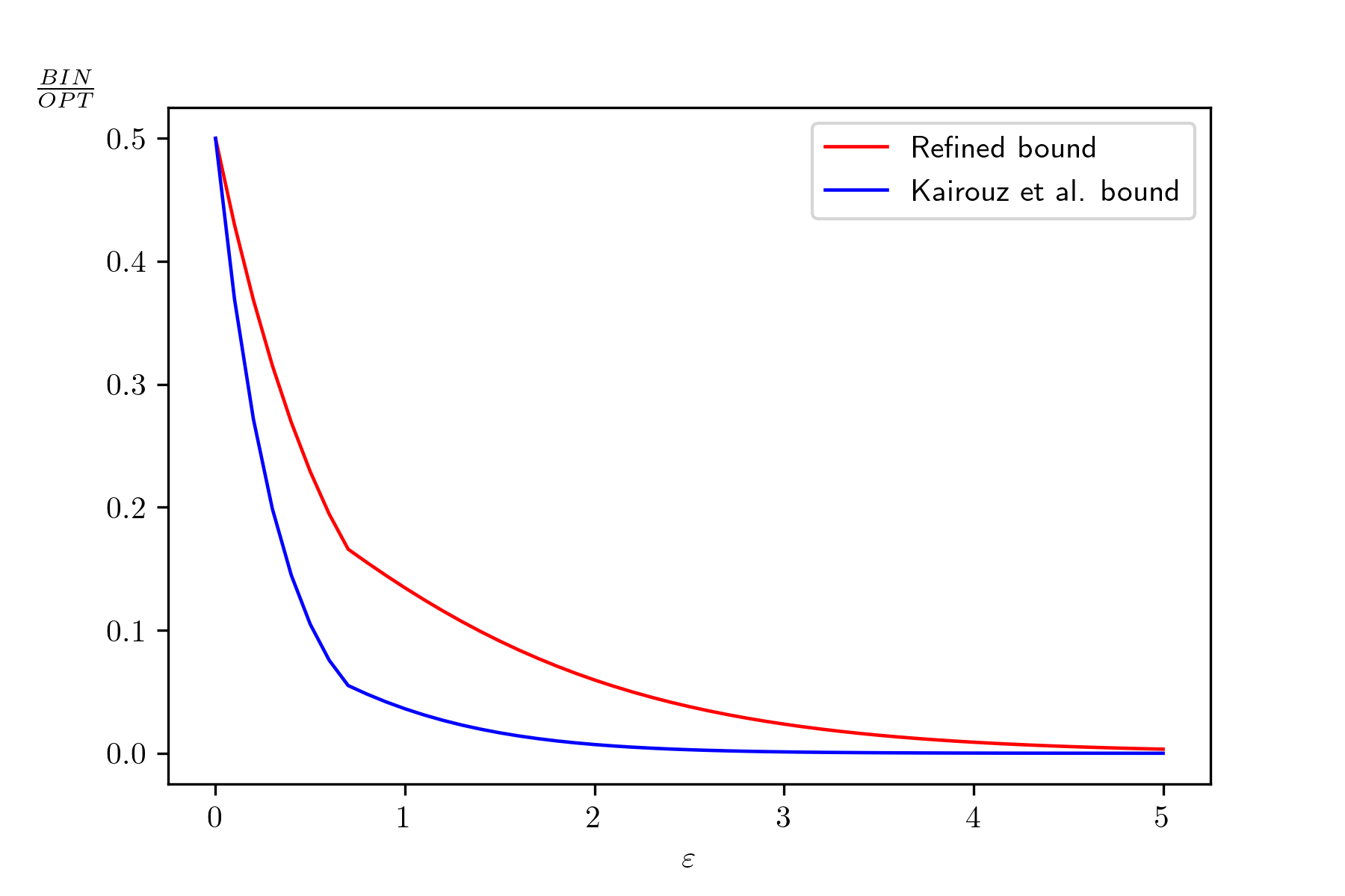
Figure 5: Comparing Binary Mechanism Approximations

Proof: Since

$$D_{\text{kl}}(M_{0}||M_{1})+D_{\text{kl}}(M_{1}||M_{0})\leq 2\min{\{2,e^{\varepsilon}\}}\frac{(e^{\varepsilon}-1)^{2}}{e^{\varepsilon}+1}||P_{0}-P_{1}||^{2}_{\text{TV}},$$ (53)

then

OPT $$=\max_{Q:~{}Q\text{ is }\varepsilon\text{-LDP}}D_{\text{kl}}(M_{0}||M_{1})\leq 2\min{\{2,e^{\varepsilon}\}}\frac{(e^{\varepsilon}-1)^{2}}{e^{\varepsilon}+1}||P_{0}-P_{1}||^{2}_{\text{TV}}.$$ (54)

As for the binary mechanism,

$$\text{BIN}=D_{\text{KL}}(M_{0}^{B}||M_{1}^{B})\geq 2\|M_{0}^{B}-M_{1}^{B}\|_{TV}^{2}=2\bigg{(}\frac{e^{\varepsilon}-1}{1+e^{\varepsilon}}\bigg{)}^{2}||P_{0}-P_{1}||_{\text{TV}}^{2},$$ (55)

where the first inequality follows from Pinsker’s inequality, and the second equality follows from Theorem 4. Rewrite as

$$2(e^{\varepsilon}-1)||P_{0}-P_{1}||_{\text{TV}}^{2}\leq\frac{(1+e^{\varepsilon})^{2}}{e^{\varepsilon}-1}\text{BIN}.$$ (56)

Then

OPT $$\leq 2\min{\{2,e^{\varepsilon}\}}\frac{(e^{\varepsilon}-1)^{2}}{e^{\varepsilon}+1}||P_{0}-P_{1}||^{2}_{\text{TV}}$$ (57)

$$\leq\min{\{2,e^{\varepsilon}\}}(1+e^{\varepsilon})\text{BIN}.$$ (58)

VII-C From $\varepsilon$-LDP to $\varepsilon$-LDP with $\eta$-TV

Given two distributions $P_{0}$ and $P_{1}$ on $\mathcal{X}$, let

$$\mathrm{OPT}_{\varepsilon,\eta}= \max_{Q_{Y|X}}~{}D_{f}(M_{0}||M_{1})$$

$$\text{subject to }Q_{Y|X}\text{ is }\varepsilon\text{-LDP},$$

$$~{}d_{TV}(Q_{Y|X})\leq\eta,$$

and

$$\mathrm{OPT}_{\varepsilon}= \max_{Q_{Y|X}}~{}D_{f}(M_{0}||M_{1})$$

$$\text{subject to }Q_{Y|X}\text{ is }\varepsilon\text{-LDP}.$$

Clearly, $\mathrm{OPT}_{\varepsilon}\geq\mathrm{OPT}_{\varepsilon,\eta}$. Our next result proves a reverse inequality:

Theorem 8

For any $f$-divergence (where $f$ is convex and satisfies $f(1)=0$), $\epsilon\geq 0$, and $\eta\in[0,\frac{e^{\varepsilon}-1}{e^{\varepsilon}+1}]$,

$$\mathrm{OPT}_{\varepsilon,\eta}\geq\eta\frac{e^{\varepsilon}+1}{e^{\varepsilon}-1}\mathrm{OPT}_{\varepsilon}.$$ (59)

Proof:

Let $Q_{Y|X}$ be $\varepsilon$-LDP. Let $W_{\alpha}:\mathcal{Y}\to\mathcal{Y}\cup\{e\}$ be an erasure channel with parameter $\alpha$, i.e., for all $y\in\mathcal{Y}$, $W(y|y)=1-\alpha$ and $W(e|y)=\alpha$.

Let $Q^{\prime}_{Y|X}=W\circ Q_{Y|X}$. Note that for $y\in\mathcal{Y}$, $Q^{\prime}(y|x)=Q(y|x)(1-\alpha)$ for all $x\in\mathcal{X}$, and $Q(e|x)=\sum_{y\in\mathcal{Y}}Q(y|x)W(e|y)=\alpha$ for all $x\in\mathcal{X}$.

Lemma 3

$d_{TV}(Q^{\prime}_{Y|X})\leq(1-\alpha)\frac{e^{\varepsilon}-1}{e^{\varepsilon}+1}$.

Proof:

Fix $x,x^{\prime}$, and $A\subset\mathcal{Y}\cup\{e\}$. Then,

$$Q^{\prime}(A|x)-Q^{\prime}(A|x^{\prime}) =\sum_{y^{\prime}\in A}Q^{\prime}(y|x)-Q^{\prime}(y|x^{\prime})$$ (60)

$$=\sum_{y^{\prime}\in A\setminus\{e\}}(1-\alpha)(Q(y|x)-Q(y|x^{\prime}))$$ (61)

$$\leq(1-\alpha)\|Q(.|x)-Q(.|x^{\prime})\|_{TV}.$$ (62)

Taking supremum over all $x$, $x^{\prime}$, and $A$, and noting that $d_{TV}(Q)\leq\frac{e^{\varepsilon}-1}{e^{\varepsilon}+1}$ (by Proposition 2), we get the desired result. ∎

As such, choosing $\alpha=1-\eta\frac{e^{\varepsilon}+1}{e^{\varepsilon}-1}$, we get $Q^{\prime}$ satisfying $d_{TV}(Q^{\prime})\leq\eta$. It is straightforward to check that $Q^{\prime}$ also satisfies $\varepsilon$-LDP so that $Q^{\prime}$ is feasible for the $\mathrm{OPT}_{\varepsilon,\eta}$ problem. Let $M_{0}^{\prime}$ and $M_{1}^{\prime}$ be the induced marginals. Then,

$$M_{0}^{\prime}(e)=\sum_{x\in\mathcal{X}}P_{0}(x)Q^{\prime}(e|x)=\alpha,$$ (63)

and for all $y\in\mathcal{Y}$,

$$M_{0}^{\prime}(y)=\sum_{x\in\mathcal{X}}P_{0}(x)Q^{\prime}(y|x)=\sum_{x\in\mathcal{X}}P_{0}(x)(1-\alpha)Q(y|x)=(1-\alpha)M_{0}(y).$$ (64)

Analogous equations hold for $M_{1}^{\prime}.$ Hence,

$$D_{f}(M_{0}^{\prime}||M_{1}^{\prime}) =\sum_{y^{\prime}\in\mathcal{Y}\cup\{e\}}M_{1}^{\prime}(y)f\left(\frac{M_{0}^{\prime}(y)}{M_{1}^{\prime}(y)}\right)$$ (65)

$$=\sum_{y\in\mathcal{Y}}(1-\alpha)M_{1}(y)f\left(\frac{M_{0}(y)}{M_{1}(y)}\right)+M_{1}(e)f\left(\frac{M_{0}(e)}{M_{1}(e)}\right)$$ (66)

$$\stackrel{{\scriptstyle\text{(a)}}}{{=}}(1-\alpha)D_{f}(M_{0}||M_{1})$$ (67)

$$\stackrel{{\scriptstyle\text{(b)}}}{{=}}\eta\frac{e^{\varepsilon}+1}{e^{\varepsilon}-1}D_{f}(M_{0}||M_{1}),$$ (68)

where (a) follows from the fact that $f(1)=0$, and (b) follows from the choice of $\alpha=1-\eta\frac{e^{\varepsilon}+1}{e^{\varepsilon}-1}$. Finally, taking supremum on both sides yields

$$\mathrm{OPT}_{\varepsilon,\eta}\geq\eta\frac{e^{\varepsilon}+1}{e^{\varepsilon}-1}\mathrm{OPT}_{\varepsilon}.$$ (69)

∎

-D Proof for Approximate Differential Privacy

The following mechanism outputs an integer sampled from $P_{0}$ when the true database is $D_{0}$ (null hypothesis) and from $P_{1}$ when the true database is $D_{1}$ (alternative hypothesis). For $\varepsilon\geq 0$, $\delta>0$, and $\alpha\in[0,1]$:

$$P_{0}=\begin{cases}\delta&\text{for }x=0,\\ \frac{(1-\delta)(1-\alpha)e^{\varepsilon}}{(1+e^{\varepsilon})}&\text{for }x=1,\\ \alpha(1-\delta)&\text{for }x=2,\\ \frac{(1-\delta)(1-\alpha)}{(1+e^{\varepsilon})}&\text{for }x=3,\\ 0&\text{for }x=4,\end{cases}$$ (70)

and

$$P_{1}=\begin{cases}0&\text{for }x=0,\\ \frac{(1-\delta)(1-\alpha)}{(1+e^{\varepsilon})}&\text{for }x=1,\\ \alpha(1-\delta)&\text{for }x=2,\\ \frac{(1-\delta)(1-\alpha)e^{\varepsilon}}{(1+e^{\varepsilon})}&\text{for }x=3,\\ \delta&\text{for }x=4.\end{cases}$$ (71)

The total variation of the above mechanism is $d_{TV}=\delta+\frac{(1-\delta)(1-\alpha)(e^{\varepsilon}-1)}{1+e^{\varepsilon}}$. Setting $\alpha=0$ yields the same mechanism proposed in [6].

The proof is analogous to case of $\delta=0$ in Section III-B2. To see how the expression $\max_{\begin{subarray}{c}S\in\mathcal{X}^{k}\end{subarray}}\{\tilde{P_{0}}(S)-e^{\varepsilon_{j}}\tilde{P_{1}}(S)\}=1-(1-\delta)^{k}(1-\delta_{j})$ in Theorem 2 was derived, we split it into two parts ($p_{1}+p_{2}$), such that $p_{1}=1-(1-\delta)^{k}$ and $p_{2}=(1-\delta)^{k}\delta_{j}$.
We are interested in the sequences $s_{k}$ that achieve the inequality $\tilde{P_{0}}(s_{k})-e^{\tilde{\varepsilon}}\tilde{P_{1}}(s_{k})>0$:

• $p_{1}$: This inequality is satisfied for all output sequences in which $x=0$ appears at least once, because the probability of such a sequence under $P_{1}$ is always 0. The probability of obtaining a sequence with no “$0$”s under $P_{0}$ is $(1-\delta)^{k}$. Taking the complement to obtain the probability that a sequence contains at least one “$0$” under $P_{0}$, we get $p_{1}=1-(1-\delta)^{k}$.

• $p_{2}$: We now consider the sequences that do not contain a “$0$” and that lead to a positive $\tilde{P_{0}}(s_{k})-e^{\tilde{\varepsilon}}\tilde{P_{1}}(s_{k})$. We apply the same logic that we followed in the case of $\delta=0$. Factoring out $(1-\delta)^{k}$ from the result, we obtain $p_{2}=(1-\delta)^{k}\delta_{j}$.

-E Proof of Theorem 3

The theorem is an application of Dong et al.’s result, in particular Theorem 3.5 in “Gaussian Differential Privacy” [5], specialized for $\varepsilon$-DP and $\eta$-TV. Note that, by definition, $M_{ni}$ is $f_{\varepsilon_{ni},0,\eta_{ni}}$-DP. Now, following the definitions in [5],

$$kl(f_{\varepsilon,0,\eta}) \vcentcolon=-\int_{0}^{1}\log\left|f_{\varepsilon,0,\eta}^{\prime}(t)\right|dt$$

$$=-\left(\int_{0}^{\frac{\eta}{e^{\varepsilon}-1}}\varepsilon dt+\int_{1-\eta\frac{e^{\varepsilon}}{e^{\varepsilon}+1}}^{1}(-\varepsilon)dt\right)$$

$$=\varepsilon\eta.$$ (72)

Similarly,

$$\kappa_{2}(f_{\varepsilon,0,\eta})\vcentcolon=\int_{0}^{1}\log^{2}\left|f_{\varepsilon,0,\eta}^{\prime}(t)\right|dt=\eta\varepsilon^{2}\frac{e^{\varepsilon}+1}{e^{\varepsilon}-1},$$ (73)

and

$$\kappa_{3}(f_{\varepsilon,0,\eta})\vcentcolon=\int_{0}^{1}\left|\log\left|f_{\varepsilon,0,\eta}^{\prime}(t)\right|\right|^{3}dt=\eta\varepsilon^{3}\frac{e^{\varepsilon}+1}{e^{\varepsilon}-1}.$$ (74)

Now,

$$\sum_{i=1}^{n}kl(f_{\varepsilon_{ni},0,\eta_{ni}})=\sum_{i=1}^{n}\varepsilon_{ni}\eta_{ni}\rightarrow\frac{\mu^{2}}{2},$$ (75)

where the limit holds by assumption of the theorem. Similarly,

$$\max_{1\leq i\leq n}kl(f_{\varepsilon_{ni},0,\eta_{ni}})=\max_{1\leq i\leq n}\eta_{ni}\varepsilon_{ni}\leq\max_{1\leq i\leq n}\varepsilon_{ni}\rightarrow 0,$$ (76)

where the limit holds by assumption. Since $kl(f)\geq 0$, then $\max_{1\leq i\leq n}kl(f_{\varepsilon_{ni},0,\eta_{ni}})\rightarrow 0$. Moreover, note that

$$\sum_{i=1}^{n}\left|\frac{1}{2}\kappa_{2}(f_{\varepsilon_{ni},0,\eta_{ni}})-kl(f_{\varepsilon_{ni},0,\eta_{ni}})\right|$$

$$=\sum_{i=1}^{n}\varepsilon_{ni}\eta_{ni}\left|\frac{\varepsilon_{ni}(e^{\varepsilon}_{ni}+1)}{2(e^{\varepsilon}_{ni}-1)}-1\right|$$

$$\leq\sum_{i=1}^{n}\varepsilon_{ni}\eta_{ni}\varepsilon_{ni}^{2}$$

$$\leq\max_{1\leq i\leq n}\varepsilon_{ni}^{2}\sum_{i=1}^{n}\varepsilon_{ni}\eta_{ni}\rightarrow 0,$$

where the first inequality follows from the Taylor expansion of $t(e^{t}+1)/(e^{t}-1)$. Hence,

$$\sum_{i=1}^{n}\kappa_{2}(f_{\varepsilon_{ni},0,\eta_{ni}})\rightarrow\mu^{2}.$$ (77)

Similarly, one can show that $\sum_{i=1}^{n}\kappa_{3}(f_{\varepsilon_{ni},0,\eta_{ni}})\rightarrow 0$. Coupled with equations (75), (76), and (77), the assumptions of Theorem 3.5 of [5] are satisfied, hence the limit of the composition converges uniformly to $G_{\mu}$.

-F Proof of Proposition 1

Since $M$ is $(\varepsilon,\delta)$-DP then $M\circ\mathrm{Sample}_{m}$ is ($\log\left(1+p\left(e^{\varepsilon}-1\right)\right),p\delta$)-DP by Theorem 29 of [18]. Similarly, $M$ being $\eta$-TV can be rewritten as $(0,\eta)$-DP (see, for instance, equations of Corollary 1). Hence, $M\circ\mathrm{Sample}_{m}$ is ($0$,$p\eta$)-DP, i.e., it’s $p\eta$-TV, as desired.

-G Total Variation of the Laplace Mechanism

To determine the total variation of the Laplace mechanism, consider two Laplace distributions, one centered at zero ($P:Lap(\frac{1}{\varepsilon},0)$), and one shifted to the right by the sensitivity ($Q:Lap(\frac{1}{\varepsilon},\Delta)$).

$$d_{TV}(P,Q) =\int_{x:P(x)>Q(x)}P(x)-Q(x)\,dx$$

$$=\int_{-\infty}^{\Delta/2}\frac{\varepsilon}{2\Delta}e^{-\frac{\varepsilon|x|}{\Delta}}-\frac{\varepsilon}{2\Delta}e^{-\frac{\varepsilon|x-\Delta|}{\Delta}}\,dx$$

$$=\int_{-\infty}^{0}\frac{\varepsilon}{2\Delta}(e^{\varepsilon x}-e^{-\varepsilon(\Delta-x)})\,dx$$

$$~{}~{}+\int_{0}^{\frac{\Delta}{2}}\frac{\varepsilon}{2\Delta}(e^{-\varepsilon x}-e^{-\varepsilon(\Delta-x)})\,dx$$

$$=1-e^{-\frac{\varepsilon}{2}}.$$

-H Total Variation of the Gaussian Mechanism

Corollary $2.13$ in [5] states that a mechanism is $\mu$-GDP if and only if it is ($\varepsilon$,$\delta(\varepsilon)$)-DP for all $\varepsilon\geq 0$, where $\delta(\varepsilon)=\Phi\bigl{(}-\frac{\varepsilon}{\mu}+\frac{\mu}{2}\bigr{)}-e^{\varepsilon}\Phi\bigl{(}-\frac{\varepsilon}{\mu}-\frac{\mu}{2}\bigr{)}$. Thus, the total variation distance of the Gaussian mechanism is

$$\delta(0)=\Phi\bigl{(}\frac{\mu}{2}\bigr{)}-\Phi\bigl{(}-\frac{\mu}{2}\bigr{)}=2\Phi\bigl{(}\frac{\mu}{2}\bigr{)}-1.$$ (78)

-I Analysis of the Staircase Mechanism

-I1 Total Variation

To derive the total variation of the staircase mechanism, we consider two distributions: $P(x)$ centered at $0$, and $Q(x)$, which is $P(x)$ shifted to the right by the sensitivity $\Delta$. We obtain the total variation of the staircase mechanism by subtracting the areas under each distribution for the values of $x$ where $P(x)>Q(x)$.
We distinguish the cases of $\gamma\leq\frac{1}{2}$ and $\gamma>\frac{1}{2}$.
For $\gamma\leq\frac{1}{2}$, we are interested in the interval $(-\infty,\gamma]$ which we split into two sub-intervals (Figure 6):

• For $(-\infty,-\gamma]$, the difference between the area under the red curve and that under the blue curve is given by $a(\gamma)\Delta\sum_{n=1}^{\infty}{(e^{-n\varepsilon}-e^{-n\varepsilon-\varepsilon})}=a(\gamma)\Delta e^{-\varepsilon}$

• For $(-\gamma,\gamma]$, the difference is $a(\gamma)(2\gamma\Delta(1-e^{\varepsilon}))$

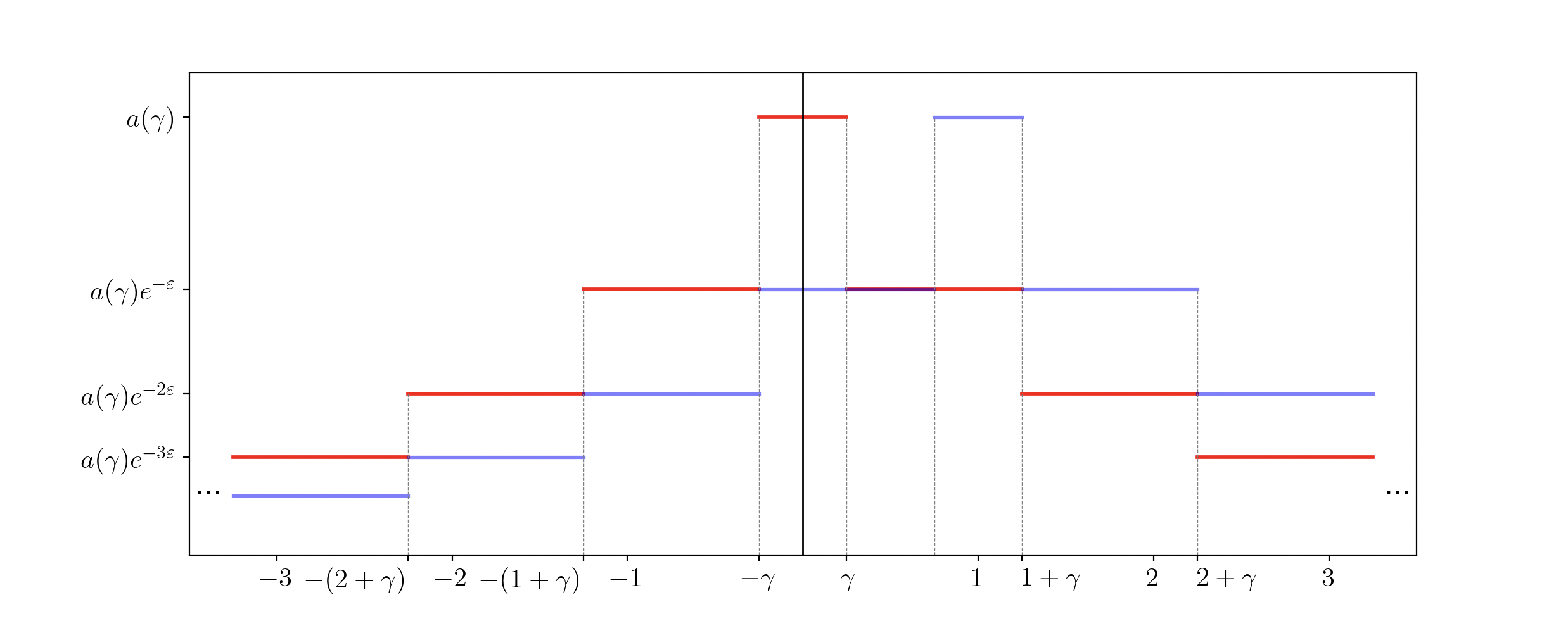
Figure 6: Two staircase distributions for $\gamma\leq\frac{1}{2}$ shifted by the sensitivity.

For $\gamma>\frac{1}{2}$, we look at the interval $(-\infty,1-\gamma)$ (Figure 7). The total variation of the mechanism is given by $a(\gamma)\Delta\sum_{n=0}^{\infty}{(e^{-n\varepsilon}-e^{-n\varepsilon-\varepsilon})}=a(\gamma)\Delta$.

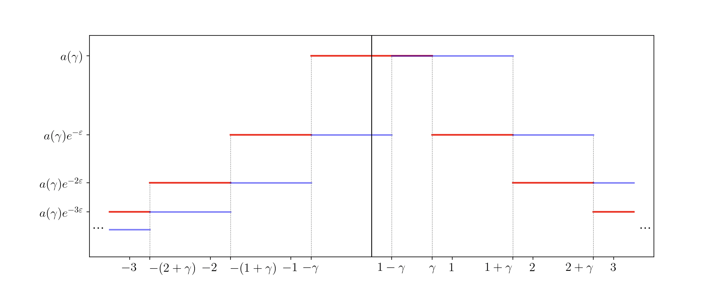
Figure 7: Two staircase distributions for $\gamma>\frac{1}{2}$ shifted by the sensitivity.

Considering two intervals for the values of $\gamma$ and setting $\Delta=1$, we derive the following expressions for the total variation of the staircase mechanism

$$d_{TV}\!\!=\!\!\left\{\begin{aligned} &\frac{(1-e^{-\varepsilon})(2\gamma(1-e^{-\varepsilon})+e^{-\varepsilon})}{2(\gamma+e^{-\varepsilon}(1-\gamma))},&\gamma\in[0,\frac{1}{2}),\\ &\frac{1-e^{-\varepsilon}}{2(\gamma+e^{-\varepsilon}(1-\gamma))},&\gamma\in[\frac{1}{2},\infty).\end{aligned}\right.$$

-I2 Privacy Region

The staircase mechanism with total variation $\eta$ achieves exactly the privacy region corresponding to $(\varepsilon,0)$-DP $\eta$-TV (cf. Corollary 1). Consider two staircase-shaped distributions, $P_{0}$ and $P_{1}$ (where $P_{1}$ is $P_{0}$ shifted by $\Delta$) for some arbitrary $\gamma$. The Neyman-Pearson Lemma states that the optimal decision rule is to reject when the likelihood ratio is above some threshold $T$. Since the likelihood ratio of $P_{1}$ to $P_{0}$ is non-decreasing (cf. Figures 6 and 7 in Appendix -I1), we can pick a point $t$ and accept whenever $t>x$. The rejection rules $x\geq 1-\gamma$ and $x\geq\gamma$ will yield type I and II values that correspond to the points ($\frac{\eta}{e^{\varepsilon}-1}$,$1-\frac{\eta e^{\varepsilon}}{e^{\varepsilon}-1}$) and ($1-\frac{\eta e^{\varepsilon}}{e^{\varepsilon}-1}$, $\frac{\eta}{e^{\varepsilon}-1}$) in Figure 2 for $\delta=0$. The rest of the tradeoff function is derived by averaging. Therefore, the bound provided in Theorem 2 exactly describes the privacy region of the composed staircase mechanism.

-J Proof of Proposition 2

By Definition 7, it suffices to consider binary-input channels $Q_{Y|X}$ (i.e., $\mathcal{X}=\{x_{0},x_{1}\}$). In this case, Barthe and Köpf showed that [26, Corollary 1]

$$\mathrm{ML}(Q_{Y|X}):=\sum_{y}\max_{x\in\{x_{0},x_{1}\}}Q_{Y|X}(y|x)\leq\log\frac{2\varepsilon}{e^{\varepsilon}+1}.$$ (79)

Now note that $\mathrm{ML}(Q_{Y|X})$ is equivalent to Sibson mutual information of order $\infty$ [27, 28]: $I_{\infty}(X;Y)=\mathrm{ML}(Q_{Y|X})$. Moreover, Sibson showed that in the binary case,

$$d_{TV}(Q(.|X=x_{0}),Q(.|X=x_{1}))=1-e^{-I_{\infty}(X;Y)}.$$ (80)

Combining the above equations, we get

$$d_{TV}(Q(.|X=x_{0}),Q(.|X=x_{1}))=1-e^{-I_{\infty}(X;Y)}=1-e^{-\mathrm{ML}(Q_{Y|X})}\leq 1-\frac{2\varepsilon}{e^{\varepsilon}+1}=\frac{e^{\varepsilon}-1}{e^{\varepsilon}+1}.$$ (81)

References

- [1] C. Dwork, F. McSherry, K. Nissim, and A. Smith, “Calibrating noise to sensitivity in private data analysis,” in Theory of Cryptography: Third Theory of Cryptography Conference, TCC 2006, New York, NY, USA, March 4-7, 2006. Proceedings 3. Springer, 2006, pp. 265–284.
- [2] C. Dwork, K. Kenthapadi, F. McSherry, I. Mironov, and M. Naor, “Our data, ourselves: Privacy via distributed noise generation,” in Annual International Conference on the Theory and Applications of Cryptographic Techniques. Springer, 2006, pp. 486–503.
- [3] I. Mironov, “Rényi differential privacy,” in 2017 IEEE 30th Computer Security Foundations Symposium (CSF). IEEE, 2017, pp. 263–275.
- [4] C. Dwork and G. N. Rothblum, “Concentrated differential privacy,” arXiv preprint arXiv:1603.01887, 2016.
- [5] J. Dong, A. Roth, and W. J. Su, “Gaussian differential privacy,” 2019. [Online]. Available: https://arxiv.org/abs/1905.02383
- [6] P. Kairouz, S. Oh, and P. Viswanath, “The composition theorem for differential privacy,” in International conference on machine learning. PMLR, 2015, pp. 1376–1385.
- [7] J. C. Duchi, M. I. Jordan, and M. J. Wainwright, “Local privacy, data processing inequalities, and statistical minimax rates,” 2014.
- [8] P. Kairouz, S. Oh, and P. Viswanath, “Extremal mechanisms for local differential privacy,” in Advances in Neural Information Processing Systems, Z. Ghahramani, M. Welling, C. Cortes, N. Lawrence, and K. Weinberger, Eds., vol. 27. Curran Associates, Inc., 2014. [Online]. Available: https://proceedings.neurips.cc/paper_files/paper/2014/file/86df7dcfd896fcaf2674f757a2463eba-Paper.pdf
- [9] Q. Geng, P. Kairouz, S. Oh, and P. Viswanath, “The staircase mechanism in differential privacy,” IEEE Journal of Selected Topics in Signal Processing, vol. 9, no. 7, pp. 1176–1184, 2015.
- [10] B. Rassouli and D. Gündüz, “Optimal utility-privacy trade-off with total variation distance as a privacy measure,” IEEE Transactions on Information Forensics and Security, vol. 15, pp. 594–603, 2019.
- [11] M. Yaghini, B. Kulynych, and C. Troncoso, “Disparate vulnerability: on the unfairness of privacy attacks against machine learning,” CoRR, vol. abs/1906.00389, 2019. [Online]. Available: http://arxiv.org/abs/1906.00389
- [12] L. Wasserman and S. Zhou, “A statistical framework for differential privacy,” Journal of the American Statistical Association, vol. 105, no. 489, pp. 375–389, 2010.
- [13] D. Blackwell, “Equivalent comparisons of experiments,” The annals of mathematical statistics, pp. 265–272, 1953.
- [14] T. M. Cover and J. A. Thomas, “Elements of information theory 2nd edition,” Willey-Interscience: NJ, 2006.
- [15] S. P. Kasiviswanathan, H. K. Lee, K. Nissim, S. Raskhodnikova, and A. Smith, “What can we learn privately?” SIAM Journal on Computing, vol. 40, no. 3, pp. 793–826, 2011.
- [16] A. Smith, “Differential privacy and the secrecy of the sample,” Sep 2009. [Online]. Available: https://adamdsmith.wordpress.com/2009/09/02/sample-secrecy/
- [17] K. Chaudhuri and N. Mishra, “When random sampling preserves privacy,” in Advances in Cryptology - CRYPTO 2006, C. Dwork, Ed. Berlin, Heidelberg: Springer Berlin Heidelberg, 2006, pp. 198–213.
- [18] T. Steinke, “Composition of differential privacy & privacy amplification by subsampling,” arXiv preprint arXiv:2210.00597, 2022.
- [19] A. Koskela, J. Jälkö, L. Prediger, and A. Honkela, “Tight differential privacy for discrete-valued mechanisms and for the subsampled gaussian mechanism using fft,” in Proceedings of The 24th International Conference on Artificial Intelligence and Statistics, ser. Proceedings of Machine Learning Research, A. Banerjee and K. Fukumizu, Eds., vol. 130. PMLR, 13–15 Apr 2021, pp. 3358–3366. [Online]. Available: https://proceedings.mlr.press/v130/koskela21a.html
- [20] S. Gopi, Y. T. Lee, and L. Wutschitz, “Numerical composition of differential privacy,” in Advances in Neural Information Processing Systems, M. Ranzato, A. Beygelzimer, Y. Dauphin, P. Liang, and J. W. Vaughan, Eds., vol. 34. Curran Associates, Inc., 2021, pp. 11 631–11 642. [Online]. Available: https://proceedings.neurips.cc/paper_files/paper/2021/file/6097d8f3714205740f30debe1166744e-Paper.pdf
- [21] Y. Zhu, J. Dong, and Y.-X. Wang, “Optimal accounting of differential privacy via characteristic function,” in Proceedings of The 25th International Conference on Artificial Intelligence and Statistics, ser. Proceedings of Machine Learning Research, G. Camps-Valls, F. J. R. Ruiz, and I. Valera, Eds., vol. 151. PMLR, 28–30 Mar 2022, pp. 4782–4817. [Online]. Available: https://proceedings.mlr.press/v151/zhu22c.html
- [22] Q. Geng and P. Viswanath, “The optimal mechanism in differential privacy,” in 2014 IEEE International Symposium on Information Theory, 2014, pp. 2371–2375.
- [23] R. L. Dobrushin, “Central limit theorem for nonstationary markov chains. i,” Theory of Probability & Its Applications, vol. 1, no. 1, pp. 65–80, 1956.
- [24] S. Asoodeh, M. Aliakbarpour, and F. P. Calmon, “Local differential privacy is equivalent to contraction of an -divergence,” in 2021 IEEE International Symposium on Information Theory (ISIT). IEEE, 2021, pp. 545–550.
- [25] B. Zamanlooy and S. Asoodeh, “Strong data processing inequalities for locally differentially private mechanisms,” in 2023 IEEE International Symposium on Information Theory (ISIT). IEEE, 2023, pp. 1794–1799.
- [26] G. Barthe and B. Kopf, “Information-theoretic bounds for differentially private mechanisms,” in 2011 IEEE 24th Computer Security Foundations Symposium. IEEE, 2011, pp. 191–204.
- [27] R. Sibson, “Information radius,” Zeitschrift für Wahrscheinlichkeitstheorie und verwandte Gebiete, vol. 14, no. 2, pp. 149–160, 1969.
- [28] S. Verdú, “-mutual information,” in 2015 Information Theory and Applications Workshop (ITA). IEEE, 2015, pp. 1–6.