Divergent Token Metrics: Measuring degradation to
prune away LLM components – and optimize quantization

Abstract

Large Language Models (LLMs) have reshaped natural language processing with their impressive capabilities. Their ever-increasing size, however, raised concerns about their effective deployment and the need for LLM compressions. This study introduces the Divergent Token metrics (DTMs), a novel approach for assessing compressed LLMs, addressing the limitations of traditional perplexity or accuracy measures that fail to accurately reflect text generation quality. DTMs focus on token divergence, that allow deeper insights into the subtleties of model compression, i.p. when evaluating component’s impacts individually. Utilizing the First Divergent Token metric (FDTM) in model sparsification reveals that a quarter of all attention components can be pruned beyond 90% on the Llama-2 model family, still keeping SOTA performance. For quantization FDTM suggests that over 80% of parameters can naively be transformed to int8 without special outlier management. These evaluations indicate the necessity of choosing appropriate compressions for parameters individually—and that FDTM can identify those—while standard metrics result in deteriorated outcomes.

Divergent Token Metrics: Measuring degradation to
prune away LLM components – and optimize quantization

Björn Deiseroth^1,2,3,∗                        Max Meuer¹                        Nikolas Gritsch^1,4                        Constantin Eichenberg¹

Patrick Schramowski^2,3,5                        Matthias Aßenmacher^4,6                        Kristian Kersting^{2,3,5 1} Aleph Alpha ² Technical University Darmstadt ³ Hessian Center for Artificial Intelligence (hessian.AI) ⁵ German Center for Artificial Intelligence (DFKI) ⁴ Department of Statistics, LMU ⁶ Munich Center for Machine Learning (MCML)

1 Introduction

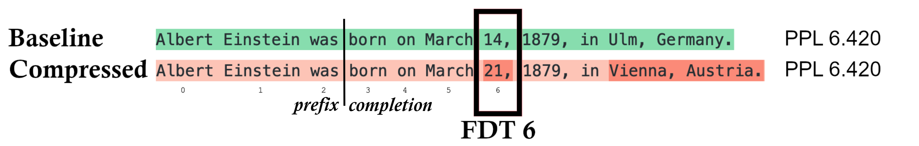
Figure 1: Illustration of a diverging generation process. Given the 3-token prefix as prompt, a base and its compressed model generate 8 subsequent tokens. Our proposed metric points to the first divergent token (FDT). The FDT may cause further divergence during the iterative generation process. Note how both models score the same perplexity value, as the actual sampling process is not reflected (c.f. Fig. 2, Sec. 4 for an empirical exploration).

Cutting-edge Large Language Models (LLMs) based on the transformer architecture have revolutionized Natural Language Processing with their exceptional performance, notably exemplified by the GPT-series (Radford et al., 2018, 2019; Brown et al., 2020; Bubeck et al., 2023; OpenAI, 2022) in text generation. However, these models have grown vastly massive, even exceeding half a trillion parameters Chowdhery et al. (2022). While their bountiful parameters aid early training convergence, their practical utility and true necessity remain unclear.

Compression strategies like sparsification and quantization can enhance parameter efficiency. Current metrics, however, are either averaging too coarsely, such as perplexity, or are by design too specific, such as standard NLP benchmarks. Either fail to capture the diverging performance nuances introduced by the compression early on. As they oversight the actual discontinous text generation process. This however is the main use of the final model, and we thus argue, that they are therefore insufficient measures for the performance of compressed model. This misalignment can lead to unwanted subtle discrepancies in generations, such as grammatical errors or a mismatch in numbers as we will see, even when overall metrics, such as perplexity, appear satisfactory (cf. Prop. 3.2, Sec. 4). An example is depicted in Fig. 1.

To meet these challenges, we introduce the family of Divergent Token metrics (DTMs). These metrics are tailored to measure the model divergence of LLMs throughout the compression process and in relation to the actual generation procedure. We demonstrate that the First Divergent Token metric (FDTM) and the Share of Divergent Tokens metric (SDTM) offer a more nuanced evaluation compared to perplexity. They, moreover, enable an individual component evaluation to rank parts of the model best suited for compression, thus enabling meaningful compression while preserving text generation quality. Specifically, sparsification enhanced by FDTM indicates significant differences in component utilization across layers. For the first time, we show that almost twenty percent of the model components can be pruned beyond 90%, several even entirely removed, while preserving a single-digit perplexity. Consequently, one can employ a sparse matrix format to accelerate computational efficiency. Likewise for precision reduction we show that sorting components by FDTM coincidentally correlates to sorting by their induced number of outliers when being converted to int8. FDTM identifies the optimal 80% of components that overall keep performance without specific outlier-handling. The observed decline in performance with more outliers, and the significant influence of specific components on those, suggests to reevaluate the applied normalization methods throughout the model. This level of precision goes beyond what standard perplexity and conventional NLP benchmarks can achieve. As the proposed Divergent Token metrics closely reflect the generation process, and as such, can be a measure to foster confidence of deployed compressed models.

We proceed as follows. We first briefly revisit common compression principles known from the literature. Afterwards we introduce our novel family of metrics. Before concluding, we present our exhaustive experimental evaluation of sparsification and quantization.

2 Compression Principles

Model compression aims to reduce the hardware resources needed to operate the model. Indeed, doing so may sacrifice model accuracy. To keep the regret as small as possible, a corrective measure is typically used. Here, we discuss the most commonly used concepts and state-of-the-art methods for sparsification and quantization of LLMs.

Outlier and Hessians.

Most model compression methods rely either on the separation of outliers or the computation of a Hessian matrix. Outliers usually refer to significantly larger values in magnitude occurring either in the weight matrix directly or in the activations during a forward pass. As most computations are linear matrix multiplications, such outliers strongly influence the remaining entropy contained in consecutive computations. In the case of sparsification, outliers should be left intact, and the values with the least magnitude—which are consequently the least influential—should be masked instead. For quantization, it was suggested to be beneficial to separate outliers and compute parts in higher-bit formats. This is i.p. motivated due to rounding issues in lower precision formats Dettmers et al. (2022). On the other hand, after conversion, Hessian matrices can be applied. They can effectively be approximated by computing backpropagation gradients for a small number of samples and represent a second-order approximation to reconstruct the original model Frantar et al. (2023).

Sparsification.

The goal of sparsification is a reduction of the overall number of weights and as such, a distillation of the relevant computation. Typically, this category is divided into “structured” and “unstructured” pruning. Structured-pruning aims to locate dynamics, such as the irrelevance of an entire layer or dimension for a given use case and prunes these entirely. Unstructured-pruning usually refers to the masking of weights, i.e., setting the irrelevant weights to 0. High levels of sparse matrix computations could result in more efficient kernels and computations. Masks exceeding 90%, in particular, allow the transition to a specific sparse matrix format, which typically necessitates the additional storage of weight indices, but significantly enhances performance.

Magnitude pruning selects the masking of weights only based on their magnitudes. This is fast to compute but significantly degenerates model performance when pruning larger amounts simultaneously. To resolve this issue, wanda Sun et al. (2023) proposes to sample a small amount of data and incorporate activations during the forward pass. It was shown that this generates more effective one-shot pruning masks. Finally, SparseGPT Frantar and Alistarh (2023) computes iterative Hessian approximations to select the lowest impact weights and correct the remaining.

Note that the incorporation of activations can to some extent be interpreted as a milder form of training. Moreover, despite these efforts, one-shot pruning has not yet produced directly usable models without further final fine-tunings. This is in particular the case for high sparsity levels beyond 70%, that we target. Finally, the components of a model have not yet been investigated individually, at all.

Quantization.

Model quantization pertains to reducing the utilized precision in the employed numeric format. Usually, LLMs are trained in 16-bit floating-point (fp16) and converted to 8-bit integer (int8) representations. The naive solution of converting float matrices to integers is the AbsMax rounding. It divides a number by the maximum value occurring in the matrix and multiplies by the largest available integer—as such, it spans a uniform representation grid. The largest float value is stored and multiplied for dequantization. The most prominent methods to mitigate the introduced rounding errors are LLM.int8() and GPTQ.

Dettmers et al. (2022) introduced LLM.int8(), which identifies vectors containing outliers and retains them in their original fp16 form during the matrix multiplication of a forward pass. The vectors lacking outliers are quantized fully. Their int8 weights and activations during the forward pass are subsequently multiplied and dequantized afterward. This allows them to be integrated with the fp16 representation of the outliers. Through empirical investigation optimizing the trade-off between degradation in perplexity and the number of outliers preserved in fp16, they fixed an absolute outlier threshold.

The GPTQ framework offers a more robust quantization approach, i.p., to different integer bit-precision. It does not rely on any outlier detection mechanism or mixed precision computations—matrix multiplications with the weights are fully performed on integers. Frantar et al. (2023) introduce an efficient Hessian approximation and iteratively quantize the weights of the matrices while performing error corrections on the remaining weights.

3 Model Divergence Metrics

Perplexity fails to identify minor variations in model degradation at an early stage. This behavior is depicted in Fig. 1 and 2 and discussed in Sec. 3.5 and 4 in more detail. To assess model divergence and enhance the model compression process, we introduce token-based metrics specifically designed to detect those nuances occurring in early compression stages. We start by establishing our notation and presenting the perplexity metric (PPL). Subsequently, we introduce an enhanced variant of PPL and propose the Share of Divergent Tokens metric (SDTM) and First Divergent Token metric (FDTM). We conclude by discussing the advantages of each metric compared to traditional perplexity-based measures when assessing the degradation of the generative performance of compressed models.

3.1 Basic notation

Let $F$ denote an auto-regressive model over a vocabulary $\mathcal{V}=\{0,1,...,|\mathcal{V}|-1\}$, $y=(y_{1},..,y_{N})\in\mathcal{V}^{N}$ an arbitrary token sequence and $F(y)=F(y)_{ij}\in{\mathbb{R}}^{N\times|\mathcal{V}|}$ the model logits. Given a prefix length $n<N$, we denote the token prefix $y_{:n}=(y_{1},...,y_{n})$ and the greedily decoded completion up to index $N$ by $\mathcal{G}(F,y_{:n},N)$. It is defined recursively as follows: $\mathcal{G}(F,y_{:n},N)_{:n}=y_{:n}$, and for $n\leq i\leq N-1$

$$\textstyle\mathcal{G}(F,y_{:n}, N)_{i+1}$$

$$\textstyle=\operatorname*{arg\,max}_{j}F(\mathcal{G}(F,y_{:n},N)_{:i})_{ij}.$$

3.2 Perplexity (PPL)

Given a ground truth sequence $y$ and model $F$, the negative log-likelihood of $y$ given $F$ is

$$\textstyle\operatorname{NLL}(y,F, n)$$

$$\textstyle=-\frac{1}{N-n}\sum_{i=n}^{N-1}\log\mathbb{P}(y_{i+1}|y_{i},..,y_{1}),$$

with $\mathbb{P}(y_{i+1}|y_{i},..,y_{1})=(\mathrm{softmax}\ F(y))_{iy_{i+1}}$. Then the perplexity is given by

$$\operatorname{PPL}(y,F,n)=\exp(\operatorname{NLL}(y,F,n)).$$

A common practice in the literature, e.g. Dettmers et al. (2022), is to measure model degradation as the increase in average perplexity over a given test dataset $\mathcal{D}$, e.g. randomly sampled from C4 Raffel et al. (2019). Usually, this metric is computed disregarding the prefix, i.e., with $\operatorname{PPL}(y,F):=\operatorname{PPL}(y,F,1)$.

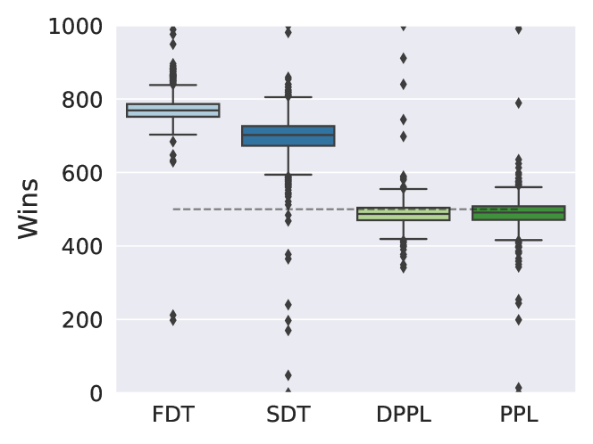
Figure 2: We test the metrics to distinguish between pruning lowest weights, and random weights. FDT is able to discriminate the cases. PPL exactly performs on the level of guessing. C.f. Sec. 4.2.

3.3 Context aware model comparison

First, we argue that standard evaluation does not reflect the typical generative model usage, i.e., there are no empty prompts, and as such, those positions should not be taken into account when evaluating the generative performance. Moreover, when comparing a compressed model $F^{\prime}$ to the original model $F$, one is rather interested to what extent the original behavior is kept. Therefore, we propose to use the outputs of the original model $F$ as a ground truth to assess the performance of the compressed model $F^{\prime}$. This leads to the definition of the divergent perplexity metric as

$$M_{\mathrm{DPPL}}(F, F^{\prime},y_{:n},N)$$ (1)

$$=\operatorname{PPL}(\mathcal{G}(F,y_{:n},N),F^{\prime},n)\;.$$

Finally, let $\mathcal{D}$ be an arbitrary test dataset containing documents of potentially varying length. For a fixed prompt length $n$ and completion length $N$, we define the aggregated divergent perplexity metric as the complete evaluation on the dataset:

$$\textstyle\mathcal{M}_{\mathrm{DPPL}}( F,F^{\prime},n,N)=$$ (2)

$$\textstyle\frac{1}{|\mathcal{D}|}\sum_{y\in\mathcal{D}}M_{\mathrm{DPPL}}(F,F^{\prime},y_{:n},N).$$

In the following, we will ease notation and omit $\mathcal{M}$, or the words aggregated and metric, when they become clear by the context. The as such denoted DPPL already substantially improves discriminative capabilities over PPL, as we will demonstrate in the empirical evaluation.

3.4 Divergent Token Metrics

SDT.

To iterate on the expressiveness and interpretability of model divergence, we propose the share of divergent tokens (SDT) as follows:

$$\textstyle\operatorname{SDT}(y, F,n)$$

$$\textstyle=|\{i\geq n\colon\ \operatorname*{arg\,max}_{j}\ F(y)_{ij}\neq y_{i+1}\}|,$$

$\operatorname{SDT}(y,F,n)$ can be interpreted as the number of times the model would need to be corrected during decoding to match the ground truth after consuming the prefix. This metric provides a more direct interpretation of the errors occurring during actual token generation, as opposed to estimating prediction certainties as PPL does.

FDT.

In addition to SDT, we introduce the first divergent token (FDT) as

$${\textstyle\operatorname{FDT}(y,F,n)}$$ (3)

$${\textstyle=\min\{i\geq n\colon\operatorname*{arg\,max}_{j}\ F(y)_{i,j}\neq y_{i+1}\}-n,}$$

with the convention that the minimum is equal to $N$ if the set on the right-hand side is empty. Analogously to Eq. 1 and Eq. 2, we define $M_{\mathrm{SDT}},M_{\mathrm{FDT}}$ and $\mathcal{M}_{\mathrm{SDT}},\mathcal{M}_{\mathrm{FDT}}$ in the same fashion.

As an illustrative example, consider to compute $M_{\mathrm{FDT}}(F,F^{\prime},y_{:n},N)$. We first perform a greedy decoding of $N-n$ tokens with the base model $F$ given the prefix $y_{:n}$. We then feed the sequence $\mathcal{G}(F,y_{:n},N)$ into the compressed model $F^{\prime}$ and find the first index greater than or equal to $n$, where the logit argmax of $F^{\prime}$ differs from what $F$ generated. This computation can be done in a single forward pass similar to perplexity, and is as such more efficient than accuracy based evaluations. Trivially, $0\leq M_{\mathrm{FDT}}(F,F^{\prime},y_{:n},N)\leq N-n$, where the upper bound is reached if and only if $F$ and $F^{\prime}$ would generate the exact same sequence up to position $N$ given the prefix $y_{:n}$. Further note that $M_{\mathrm{FDT}}$ is symmetric, i.e. $M_{\mathrm{FDT}}(F,F^{\prime},y_{:n},N)=M_{\mathrm{FDT}}(F^{\prime},F,y_{:n},N)$, in contrast to PPL.

3.5 Token vs. Perplexity Metrics

It turns out that divergent token metrics offer a superior criterion for analyzing model performance degradation compared to perplexity-based metrics, especially in the context of greedy decoding. The main reason for that is the fact that the greedy decoding operation $\mathcal{G}$ is a discontinuous function of the logits. To formalize this, let us discard the model itself and focus notation solely on the concept of logits.

Definition 3.1.

The operators and metrics from previous sections defined for models $F,F^{\prime}$ are defined for logits $l,l^{\prime}\in{\mathbb{R}}^{N\times|\mathcal{V}|}$ by replacing all occurrences of $F,F^{\prime}$ with $l,l^{\prime}$.

For example, $\mathcal{G}(l,y_{:n},N)_{i+1}=\operatorname*{arg\,max}_{j}l_{ij}$, for $n\leq i\leq N$.

Proposition 3.2.

Given any $y$, $N$ and $\varepsilon>0$ there exist logits $l,l^{\prime}\in{\mathbb{R}}^{N\times|\mathcal{V}|}$ such that

$$\textstyle|\operatorname{PPL}(y,l,1)-\operatorname{PPL}(y,l^{\prime},1)| <\varepsilon,$$

$$\textstyle M_{\mathrm{SDT}}(l,l^{\prime},y_{:1},N) =N.$$

Proof.

C.f. App. A. ∎

This means that even if the average perplexity of a compressed model matches the perplexity of the original model, the compressed model can produce a very different (and potentially worse) output when performing greedy decoding. Hence leading to a false positive. In practice, this is a severe issue since even a single diverging token can lead to a completely different subsequent output. It is illustrated in Fig. 1 and 2 and discussed in Sec. 4.2.

As described before, another option is to compute the perplexity with respect to the generated completions of the original model. This metric relates more reasonably to the share of divergent tokens:

Proposition 3.3.

The following upper bound holds:

$${\textstyle M_{\mathrm{SDT}}(l,l^{\prime},y_{:n},N)\leq\frac{N-n}{\log 2}\log M_{\mathrm{DPPL}}(l,l^{\prime},y_{:n},N).}$$

Proof.

C.f. App. A. ∎

However, a comparable lower bound does not generally hold. In fact, in the case $l=l^{\prime}$ we trivially have $M_{\mathrm{SDT}}(l,l,y_{:n},N)=0$. Further, the value of $M_{\mathrm{DPPL}}(l,l,y_{:n},N)$ can still be as high as the maximal value, which occurs when $l$ is a perfectly flat distribution at any sequence index. This could lead to a false negative signal for the generation process.

In conclusion, perplexity-based metrics suffer from false positives or false negatives when evaluating degradation of generative performance. The case for FDT and SDT is quite straightforward in that they both directly measure the difference between model outputs in a what-you-see-is-what-you-get manner.

Note that additional token-based metrics, such as the measurement of the width between erroneous predictions, can be readily formulated. These metrics may prove especially valuable when assessing potential benefits, for instance, in the context of correction-based inference strategies like speculative decoding Leviathan et al. (2023). We now empirically demonstrate the improvements of well-known compression methods using our metrics.

4 Token Metrics Improve Model Compression

Now, we will demonstrate how the proposed metric provides novel insights into the efficiency of the architecture of LLMs and serve as a benchmark for model compression. We outperform PPL as a ranking metric throughout all experiments.

More precisely, we apply component-wise probing on sparsification to determine individual sparsity rates. Interestingly, the model tends to remove components of the attention mechanism on certain layers entirely. In total 40 out of 280 components are sparsed beyond 90% and 15 removed completely. For quantization, on the other hand, we show how component selection significantly influences the overall number of model outliers. For the first time, almost 10% of model components can be converted to 4-bit integer representations without significant model degradation.

4.1 Experimental Protocol

Let us start by clarifying the experimental setup.

Test environment.

All experiments were performed on the public Llama2-7B and 13B models Touvron et al. (2023). Note, however, that we observed similar behavior amongst other decoder transformer models. It remains, i.p., throughout upscaled sizes, and smaller variations on the architecture or the training procedure.

For all experiments, we follow best practices of compression evaluations Sun et al. (2023) and randomly sampled from the C4 data Raffel et al. (2019) for training iterations. The final model evaluation utilizes the Wikitext2 dataset and standard NLP benchmarks Gao et al. (2021).

Metrics.

We apply our proposed metrics for performance evaluation as well as selection criteria.

We employ FDT, SDT, and PPL as metrics to assess the overall model divergence. When it comes to model compression, we demonstrated that both PPL and our variant DPPL typically struggle to measure minor changes adequately (cf. Sec. 3.5,4.2 and Fig. 2). On the other hand, FDT is particularly suited to describe errors for subtle model changes. Consequently, we apply FDT for model compression. In the following paragraph, we describe the selected parameters for compression using FDT in more detail.

Divergent Token Parameters.

We empirically selected hyperparameters as follows. Through preliminary sparsification experiments, we observed that the most variance is present in the 75%-quantile of FDT, as defined in Eq. 3. We denote this value by FDT₇₅. It is in the following our compare-to value.

Next, we swept over the given context prefix length $n$ of FDT and sparsification steps. Fig. 3 depicts different sparsification steps and prefix lengths on the x- and y-axis respectively. The heatmap shows the overall variance of FDT₇₅ on 5k probes. For simplicity, we fixed the prefix length to $100$ tokens, as it is most discriminative on average.

We observed that most sparsification steps introduce an error in FDT₇₅ within a range of $500$ completion tokens. Therefore, we selected $N=500$. Finally, to determine the number of probes $|\mathcal{D}|$, we compared the mean deviation against a baseline of $5000$ probes. Interestingly, it converged rather fast, and the deviation of $1000$ to $5000$ probes only differs on average by a value $4$ in mean FDT₇₅. Therefore, we selected $|\mathcal{D}|=1000$.

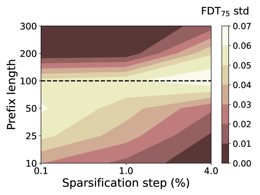
Figure 3: Hyperparameter selection of FDT. Visualized is the std in FDT₇₅ over all components when varying prefix length (y-axis) and applying different choices for sparsity-step increases (x-axis) as described in Sec. 4.1 and 4.2.

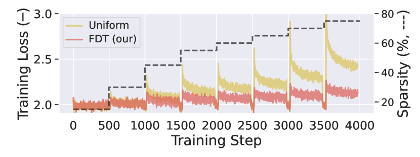
(a) Comparison of uniform and component-wise pruning using FDT as a metric for comparison.

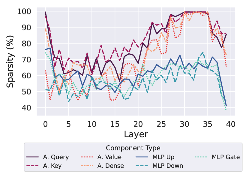
(b) Converged component config with 75% average sparsity. Layers (x-axis), Component-sparsity (y-axis).

Figure 4: Depiction of the proposed sparsification process that converged to a 75% sparse Llama-2-13b. a) Model training performance throughout all rounds. Our FDT-based sparsification clearly outperforms uniform magnitude pruning. b) Converged sparsity values per component. One quarter of attention components are pruned beyond 90% sparsity. Significant outliers appear in first and last layers.

Pruning of LLMs.

In Sec. 4.2, we will show that FDT improves sparsification procedures to achieve high compression rates on LLama2-13b.

We iterate small unstructured sparsification with continued training steps for the model to attune to the remaining weights and recover performance. Specifically, we apply eight iterations to increase the average model sparsity by $20,15,10,10,5,5,5,$ and $5$ percent. As such, the final model has 25% total parameters remaining.

We run this experiment in two configurations, uniform and FDT-selective. Uniform sparsification applies the target increase of the current round to each component uniformly, pruning the lowest weights. For FDT, we determine individual component sparsification values to evenly distribute the induced error. Based on the previous sparsed model $F$ and for the current target increase $step$, we probe each component $c_{i}$ separately with an additional $step\pm step/2$ percent of lowest weights pruned, denoted by $F^{c_{i}+s}$, to determine its FDT₇₅ value. We further add the constant extrema, i.e., step sparsity $0$ and $100\%$ with FDT₇₅ values of $500$ and $0$. Given these four data points, we segment-wise interpolate linearly to achieve the highest value of FDT₇₅ possible throughout all components, but on average yielding the target sparsity. Specifically, we find the set of component-sparsities $\{s_{i}\}$ that optimize for

$$\textstyle\operatorname*{arg\,max}_{\{s_{i}\}}\min_{i}M_{\textrm{FDT}_{75}}(F,F^{c_{i}+s_{i}}),$$

such that $\sum_{i}\tilde{s}_{i}=step$ with $\tilde{s}_{i}$ denoting the normalized sparsity of $s_{i}$ accounting the individual parameters of component $c_{i}$ in.

We further follow the findings of AC/DC Peste et al. (2021) and alternate compressed and decompressed iterations as follows: Each round we train a total of $500$ steps, from which the first 450 are with sparsification mask applied, and the following $50$ without any masks. We found this alternation to produce smaller spikes in training loss after sparsification steps. This yields a total of $4000$ training steps. During training, we apply a weight decay of $0.01$, batch size $256$, and sequence length $2048$.

Note that throughout this experiment series, we only apply pure magnitude pruning per iteration. The probing strategy can be applied to other methods, such as Wanda, as well.

Quantization of LLMs.

For model quantization, we compare the performance of the proposed metrics on the task of sorting the model’s components by their lowest introduced error. To this end, we build a search tree to find the best model configuration as follows: We construct a parallel depth-first search tree with a branching width of $10$. This means that, at each level of the tree, we simultaneously explore all possible successor configs for the currently top-$10$ performing nodes, with one more component naively quantized using AbsMax. From this newly identified set of nodes, we again select the best-performing for the next iteration. Starting with the unquantized base model Llama2-7b, each node contains exactly the number of quantized components respective to its depth, while the final node is a fully AbsMax quantized model. We further apply deduplication to prevent redundant computations.

4.2 Sparsification reveals:
        Attention is not all you need!

We applied step-wise uniform magnitude pruning, and our balanced component-wise pruning using FDT, to achieve 75% model sparsity. A summary of the results is shown in Fig. 4.

Attention almost erased.

Fig. 4(b) visualizes the converged sparsity values when applying our balanced pruning using FDT.

Notably, the model favors pruning Attention over MLP. In total 40 out of 160 attention components are sparsed beyond 90% and 15 even completely removed. In general the second half of the model appears to be more prunable than the first half. The value matrices are overall least pruned of the attention matrices. Finally, significant outliers appear at the first and last layers. This finding indicates that attention is not efficiently utilized throughout the entire model. In fact, only layers 3 to 20 and layer 40 appear to be of significant relevance for the models final prediction. This observation might be attributed to an evolving shift in distributions, and therewith the concepts processed in embeddings.

Notably, in the first layer Attention Dense and MLP Down remain significant dense, while all others are comparable sparse. This observation indicates an incomplete shift of token-embeddings.

General Observations.

As shown in Fig. 4(a), FDT based balanced pruning significantly lowers the introduced error between sparsification rounds. Uniform pruning, on the other hand, substantially diverged, and i.p. does not regain performance with the given amount of compute. Generally speaking, what is lost can hardly be recovered.

The standard evaluation of FDT and PPL on Wikitext2, is found in Tab. 1. The 75% compressed 13b model, with several components pruned away, scored PPL 8.1, compared to PPL 4.8 of the base model. Note that no other model sparsed beyond 70% has yet been reported i.p. achieving single-digit PPL. Uniform pruning achieved 13.5. Further note, that we almost doubled the mean FDT value when comparing to uniform pruning. However, as the generally low FDT value suggests, it already diverged quite far from the base model.

FDT is more discriminative.

In practice, FDT is more discriminative than PPL to subtle changes. We demonstrate this with a test as follows: On each component of the model, we prune 0.1% of the weights either randomly or from the lowest weights at a time. The resulting model is probed for $1000$ trials with all discussed metrics used to distinguish the cases. The results in Fig. 2 clearly indicate that FDT is able to distinguish the cases, while they remain indifferent for PPL-based comparison. We therefore omit using PPL as a metric to determine step-sizes for the described sparsification experiment.

In Fig. 4(b) the converged sparsity rates for all components are displayed. A final discussion of the sparsification experiment is found in App. G.

4.3 Quantization: Outliers can be prevented

Finally, we demonstrate the impact of selecting the right components on quantization. We compare the proposed metrics PPL, DPPL, and FDT as a ranking criteria to showcase their discrimation capabilities.

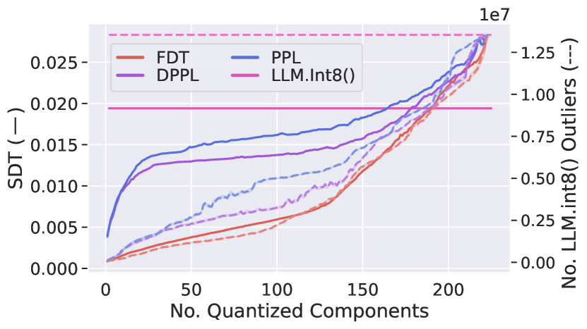
(a) Performance of FDT vs PPL

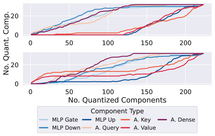
(b) Selected Components FDT vs PPL

Figure 5: Evaluation of the Tree Search as described in text. a) Comparison of Tree Search based component-wise quantization. Different number of components (x-axis) lead to different token divergence scores (y-axis, normalized to $[0,1]$), and i.p. correlates early on to introduces ouliers (second y-axis). Throughout the entire search, FDT is able to rank components by their potential errors, and, coincidentally, outliers. b) Selected components at respective depth. A.Key and A.Value induce most error.

Quantization without outlier-handling.

Fig. 5 shows the average performance of the top 10 nodes occuring in the respective search tree depth (x-axis). FDT constantly outperforms the other metrics on the Share-of-Divergent-Token metric (y-axis). Notably, this goes on par with the total number of occurring outliers for the respective configs (second y-axis). Certain components appear to significantly influence the decline observed in both measures. While DPPL enhances some aspects of performance, neither variant of PPL effectively distinguishes these components and tends to select those prematurely.

With FDT, we can cast 80%, i.e. 150, of the model’s components directly to int8 using only naive AbsMax—and without further outlier handling—still outperforming full LLM.int8() conversion in model performance. Selecting those 150 components with DPPL and FDT leads to a close perplexity scores $5.490$ and $5.489$ on Wikitext2, c.f. Tab. 1. However the resulting mean FDT improves by almost 50% when also selecting the components by this metric. The larger generation of the same sequences suggest a model closer to the original when choosing FDT as a selection criteria.

Fig. 5b) shows the selected components to each depth respective of a). Most outliers occur when selecting A. Key early on. Notably, we observed in Sec. 4.2, that this is one of the matrices most suitable to sparsify.

Sparsification
	Model	FDT $\uparrow$	PPL $\downarrow$	NLP $\uparrow$
	Llama2-13b	-	4.884	53.59
	$\sim$ 60% sparse (unif.)	004.7	09.244	46.32
	$\sim$ 60% sparse (our)	007.9	6.242	48.89
	$\sim$ 75% sparse (unif.)	00$\bullet$3.5	$\bullet$13.512	41.67
	$\sim$ 75% sparse (our)	005.5	8.101	46.32
	$\sim$ 80% sparse (our)	005.2	9.531	45.66
Quantization
	Model	FDT $\uparrow$	PPL $\downarrow$	NLP $\uparrow$
	Llama2-7b	-	5.472	50.79
int8	LLM.int8()all	036.1	5.505	50.81
	AbsMax PPL150	0$\bullet$46.3	5.500	50.72
	AbsMax DPPL150	054.1	5.490	50.75
	AbsMax FDT150 (our)	071.7	5.489	50.75
int4	GPTQall	011.1	5.665	48.34
	GPTQ PPL16	45.0	5.511	49.91
	GPTQ DPPL16	0137.0	5.476	50.02
	GPTQ FDT16 (our)	205.0	5.475	50.13

Table 1: Evals of Compressed Models. Even when evaluating the final model, standard NLP benchmarks don’t reflect the actual model degradation, as observed in AbsMax quantization. FDT, PPL are evaluated on Wikitext2. Subscript refers to best found $k$ quantized components. Bold denote best values.

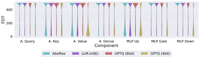
(a) Quantization methods evaluated on Components.

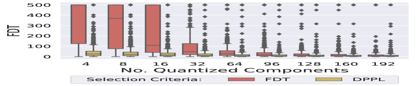
(b) Top-selected GPTQ(4bit) components.

Figure 6: Evaluation of FDT performance. a) evaluates components separately on all quantization methods. Clear outliers in performance are A.Value and MLP.up. GPTQ(8bit) is able to evenly amortize the induced error. b) Selecting top-k components of GPTQ(4bit). FDT is suited to rank components one-shot.

16 components in 4-bit.

Figure 6(a) presents a comprehensive assessment of the quantization techniques discussed. First, it is noticeable that the LLM.int8() method slightly lowers the lower quantile scores of FDT in comparison to AbsMax. Yet, GPTQ-8bit demonstrates superior performance, outshining both plain AbsMax and LLM.int8(). This method achieves a more balanced error distribution across all components (c.f. Fig. 15). Conversely, GPTQ-4bit shows noticeable deviations in the generation process, with only a limited number of components achieving FDT scores above 300. Despite this, the discriminative power of FDT enabled us to identify and merge the top 16 components that minimally compromised the model’s integrity, as illustrated in Fig. 6(b).

We conclude that PPL is not suitable for either, selecting components to compress, or for assessing the degradation of compressed models, as indicated in Table 1.

In Appendix Fig. 15 detailed FDT statistics on all components are displayed. A final discussion of the quantization experiment is found in App. B.

5 Conclusion

We introduced the Divergent Token Metrics (DTMs), a tailored approach to evaluate the performance differences of compressed generative models. In particular, DTMs respect the usually applied greedy sampling procedure to generate predictions. We proved that DTMs achieve appropriate metric bounds and are not affected from catastrophic artefacts that perplexity-based metrics encounter.

Due to our metrics’ discriminative capabilities, we are able to measure the subtle influence of model components individually, and in turn build a fine-grained selection for compression. With our sparsification experiments we achieved an outperforming 75% sparse version of the Llama2-13b model with a small amount of training steps and otherwise only applying magnitude pruning. Many (in particular attention) modules were entirely removed, which hints that attention is, after all, not always needed—during inference—in decoder models. Notably, the MLP components in the first and last layers are extremely sensitive, which hints at an incomplete shift of token-embedding distributions. For quantization, we were able to sort the influence of the quantized components individually. Interestingly sorting by FDT coincides with sorting by outliers. We successfully converted 80% of the LLama2-7b components naively to int8 using AbsMax, without severe degeneration of performance, and without any outlier-handling. Further, we concluded that GPTQ-8bit performs very well. The 4bit version, on the other hand, significantly degenerates. However, we were able to select the 16 out of 224 significantly outperforming components, that even combined, sustained substantial model performance.

Building up on this work, one could investigate further variations of our metric for specific use-cases. The average distances between falsely predicted tokens, as an example, intuitively reflect the efficiency of speculative sampling algorithms. We envision fully heterogeneous model architectures, with components mixed in precision and varying levels of sparsities. Afterall, there is ample diversity throughout the model to be exploit.

Limitations

With the proposed DTMs, compression processes can be tailored to use cases—and we can measure its performance degeneration. We hinted with the sparsification experiments, that MLP and Attention can be ascribed varying levels of significance throughout the layers. These variations should further be exploited to optimize model architectures. In particular variations of specific datasets to probe or finetune on could lead to interesting variations.

As a pruning strategy, we achieved outperforming results using only naive magnitude pruning. DTMs should directly be applicable to other masking strategies, such as Wanda Sun et al. (2023), which may further improve results. Finally, the generalizability of the metrics to other sampling strategies should be investigated.

Ethics Statement

We affirm that our research adheres to the ACL Ethics Policy. This work involves the use of publicly available data sets and does not involve human subjects or any personally identifiable information. We declare that we have no conflicts of interest that could potentially influence the outcomes, interpretations, or conclusions of this research. All funding sources supporting this study are acknowledged. We have made our best effort to document our methodology, experiments, and results accurately and are committed to sharing our code, data, and other relevant resources to foster reproducibility and further advancements in research.

Appendix

Appendix A Proof of Propositions

Proof of Proposition 3.2.

There are many ways to construct sequences that satisfy the desired relation. One is as follows: Let $l\in{\mathbb{R}}^{N\times|\mathcal{V}|}$ be any logit sequence with no re-occurring values. Denote by $m_{k}(l)_{i}$ the top-$k$ value at position $i$, and by $a_{k}(l)_{i}$ the top-$k$ vocab index at position $i$, respectively. Now we pick any such sequence with the additional property that $\max_{i}m_{1}(l)_{i}-m_{2}(l)_{i}<\delta$ for some small $\delta$. Define the sequence $l^{\prime}$ by

$$l^{\prime}_{ia_{2}(l)_{i}} =l_{ia_{2}(l)_{i}}+\delta,$$

and $l^{\prime}_{ij}=l_{ij}$ for all remaining indices. Then we have $a_{1}(l)_{i}\neq a_{1}(l^{\prime})_{i}$ for all $i$ and hence $M_{\mathrm{SDT}}(l,l^{\prime},y_{:1},N)=N$. On the other hand we have $||l-l^{\prime}||_{\infty}\leq\delta$. Since $\operatorname{PPL}(y,l,1)$ is a continuous function in $l$, we have $|\operatorname{PPL}(y,l,1)-\operatorname{PPL}(y,l^{\prime},1)|<\varepsilon$ for any $\varepsilon$ and small enough $\delta$. ∎

Proof of Proposition 3.3.

Let $z=\mathcal{G}(l,y_{:n},N)$ and $p_{i}=(\mathrm{softmax}\ l^{\prime})_{iz_{i+1}}$. Applying the definitions and elementary operations, we have

$$\sum_{i=n}^{N}-\log p_{i}=(N-n)\log M_{\mathrm{DPPL}}(l,l^{\prime},y_{:n},N).$$

Let $A=\{i\geq n\colon p_{i}\leq 1/2\}$. Then

$$\sum_{i=n}^{N}-\log p_{i} =\sum_{i\in A}-\log p_{i}+\sum_{i\in A^{c}}-\log p_{i}$$

$$\geq\sum_{i\in A}-\log p_{i}\geq|A|\log 2.$$

Here we first used that $\log p_{i}\leq 0$ and then the observation that indices contained in $A$ satisfy $-\log p_{i}\geq\log 2$ by the defining property of $A$. Finally, we argue that $\operatorname{SDT}(z,l^{\prime},n)\leq|A|$. Indeed, at any position $i$ where $\operatorname*{arg\,max}_{j}l^{\prime}_{ij}\neq z_{i+1}$ it must hold that $p_{i}\leq 1/2$, since any softmax-value larger than $1/2$ is automatically the maximum value of the distribution, and the softmax operation is monotone. Putting everything together we arrive at the desired inequality. ∎

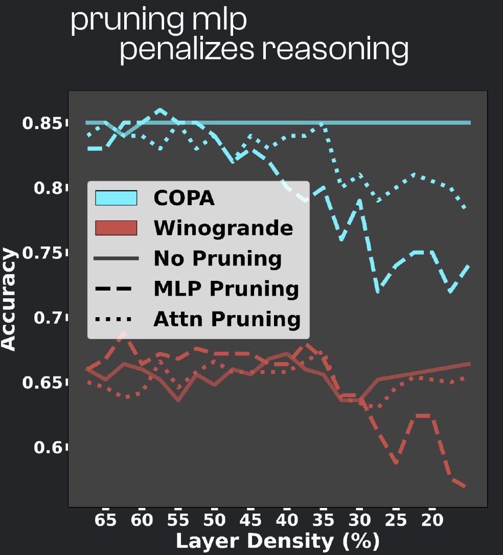
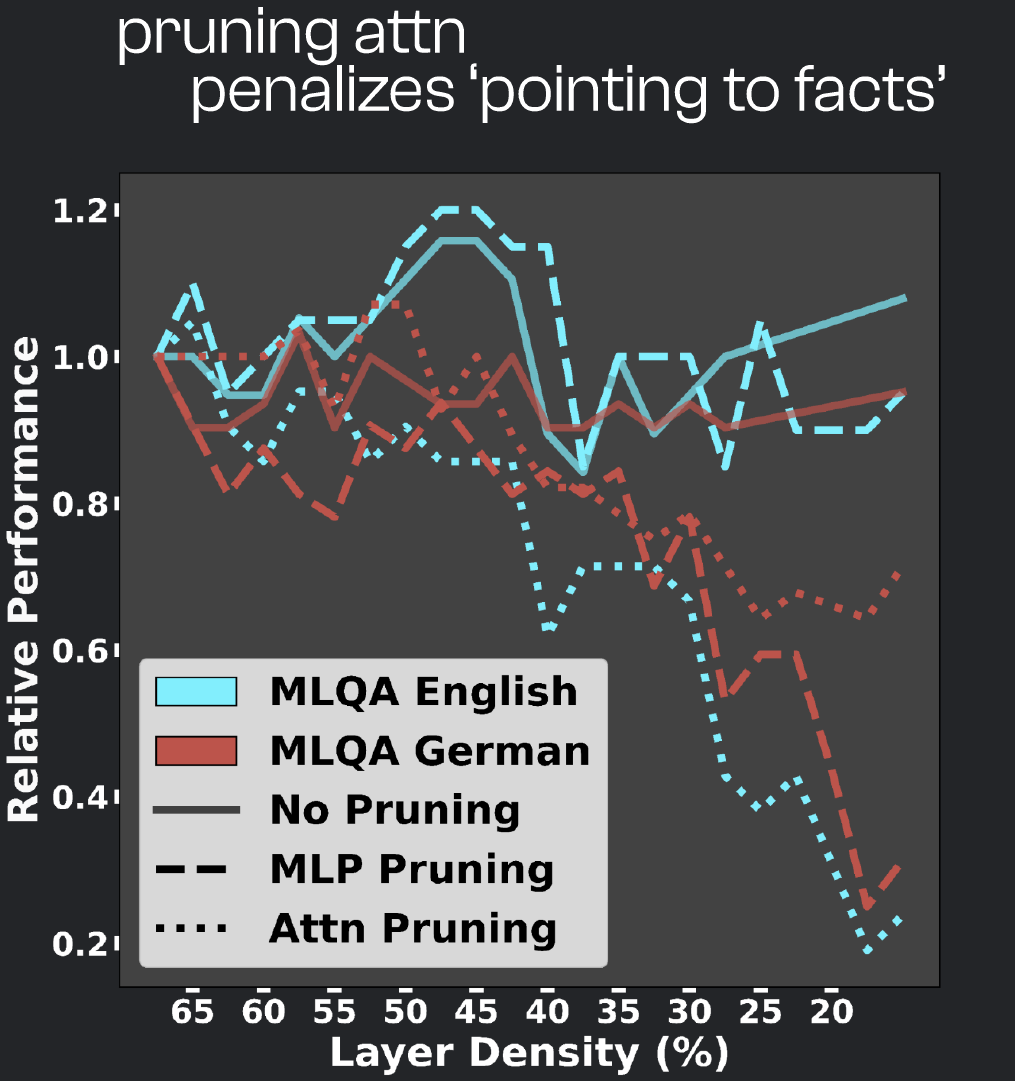
Figure 7: Pruning MLP and Attn only indeed compromises remaining model capabilities.

Appendix B FDT compared to standard model evals

Fig. 10 shows a comparison of standard benchmarks (middle) to FDT (right) and PPL (left) when quantizing parts of a model. Often standard evals fail to distinguish between compressed models. Sometimes they even depict better performance—which may be true, when regarding compression as a fine-tuning method and considering the short required token predictions. FDT thoroughly gives discriminative statistics with resprect to the base model, on how much the compressed model equals the original. Note how the error seems to be upper bounded, which suggests that errors may average out throughout the model. Mean zeroshot accuracy denotes the average on the standard NLP-eval harness.

Appendix C True positives can be predicted

Fig. 8 shows several metrics applied to the token-distributions, in order to estimate on whether the compressed and original model predictions are equal. Notably, L1 and L2 errors on the entire distribution seem to somewhat capture the discriminative capabilities of false predictions. The probability scores themselves are only marginally usable. Using top-2 uncertainty, i.e. the difference between the top-2 tokens as a measure, we obtain a reliable prediction of true positives. True negatives however still remain with a significant overlap.

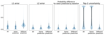
Figure 8: Top-2 uncertainty is discriminative enough to give clear true-positives estimates on compressed models.

Appendix D MLP is for knowledge,
      Attention for relation

Finally, we observed that when pruning only attention, prompt-extraction capabilities degenerate severely. When only pruning MLP components, on the other hand, it influences mostly world knowledge QA benchmarks, c.f. Fig. 7.

Appendix E Details on Search Tree, Sec. 4.3

Fig. 9 shows the layers (y-axis) of which components are selected at each round (x-axis). While there seems to be a pattern on when using FDT as a criteria (top), selection by PPL (bottom) looks more random.

Fig. 13 shows the comparison of search tree as described to greedy search on a single evaluation of all components. Until 150 components, FDT proves more stable over the PPL variants as seen in Fig. 13(a).

Figure 9: Layers selected in each round of the search tree. Top, when applying FDT, bottom, when applying PPL as a ranking metric.

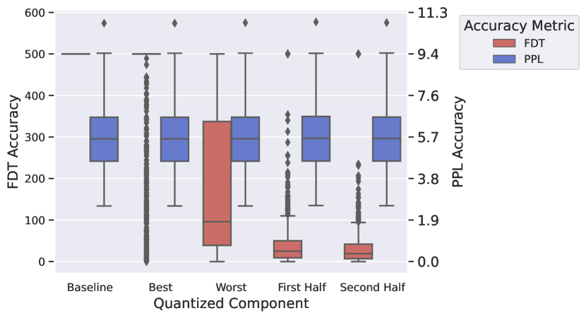
Figure 10: Comparison of the discrimination capabilities of FDT and PPL for different configurations when applying LLM.int8() conversion on Llama2-7b. Best and Worst mark a single component being converted, with most and least mean influence. First and Second half consecutively convert half of the model each. While significant changes can be observed using FDT, all configurations appear indifferent for PPL.

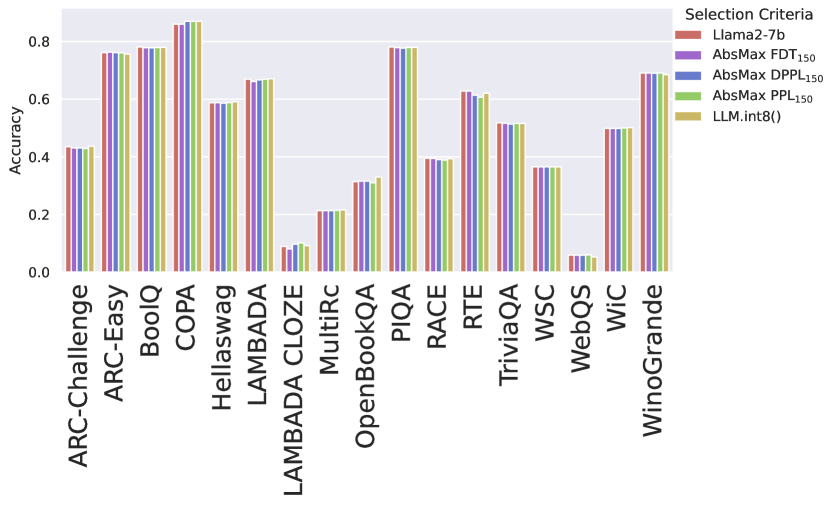
(a) 8-bit Quantization NLP benchmarks

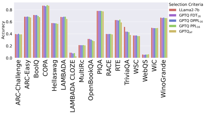
(b) 4-bit Quantization NLP benchmarks

Figure 11: Detailed view on aggregated values of Tab. 1 when selecting Llama2-7b components to quantize by metrics.

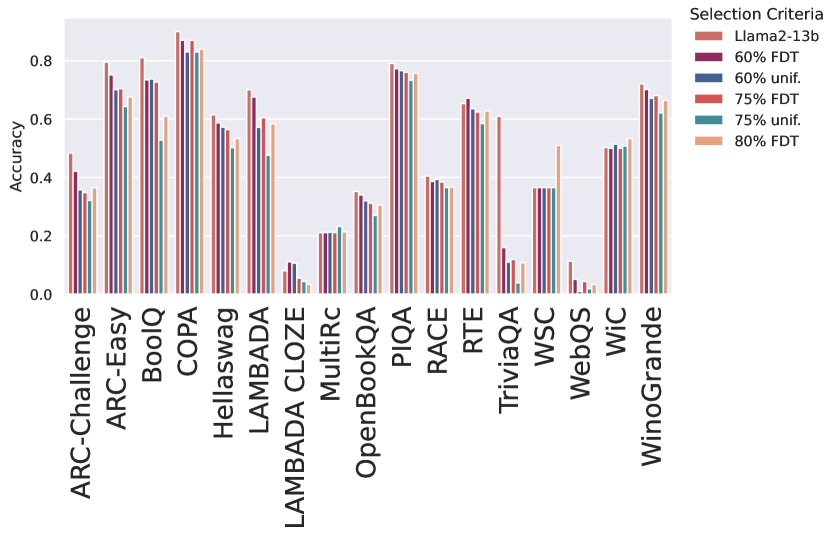
Figure 12: Detailed view on aggregated values of Tab. 1 when selecting Llama2-13b components to sparsify by metrics.

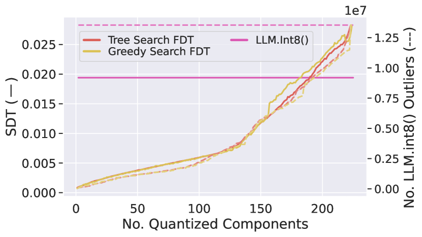
(a) FDT tree vs greedy

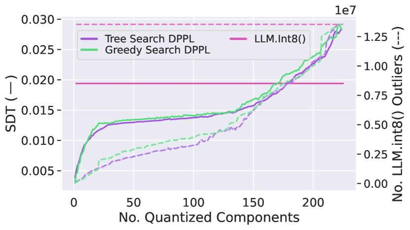
(b) DPPL tree vs greedy

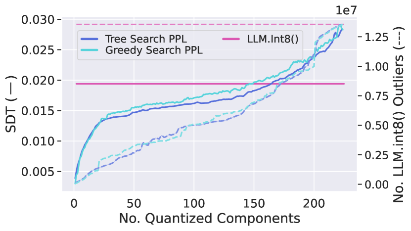
(c) PPL tree vs greedy

Figure 13: Comparison of performance when selecting components by the tree-search as described to greedy selection of once evaluated components for all discussed metrics. Clearly, FDT is most stable until 150 components.

Appendix F Details on Quantization Sec. 4.3

Fig. 15 shows detailed component-wise evaluations aggregated in Fig. 6(a).

Fig. 14 shows the final configurations as compared in Tab. 1.

Fig. 11 shows the detailed nlp-eval scores of Tab. 1.

In total the entire search evaluation required 16 GPU-days with A100s to complete all metrics.

(a) The 150 selected components selected by metrics for 8-bit AbsMax conversion.

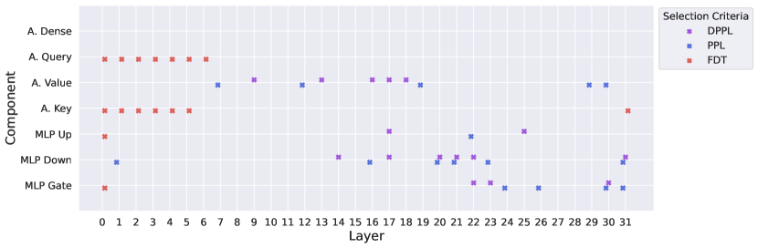
(b) The 16 selected components selected by metrics for 4-bit GPTQ conversion.

Figure 14: Detailed view of the Llama2-7b components in Tab. 1 selected by metrics for lower precision conversion.

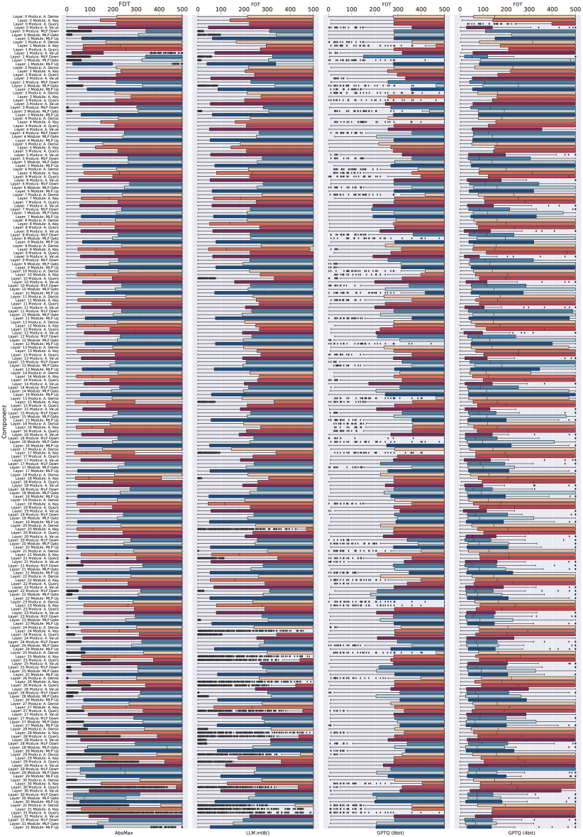
Figure 15: Full view of the influence of individual component-wise quantization measured by FDT.

Appendix G Details on Sparsification, Sec. 4.2

Fig. 16 shows a different aggregated perspective of Fig. 4(b), to point out more direct the occuring variances.

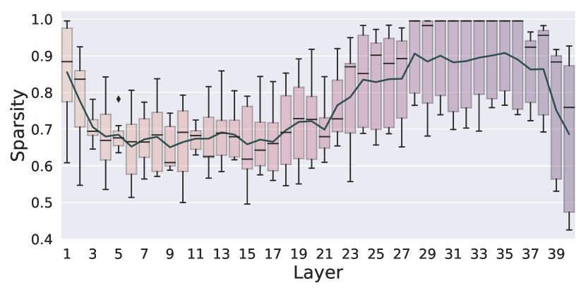
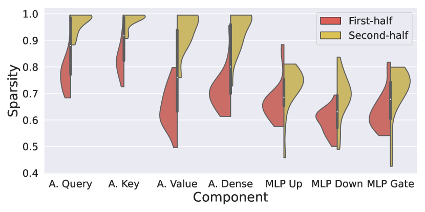
Figure 16: Distribution of 75% average model sparsity. A. denotes Attention. Top: Aggregated by layers. The first and last layer have highest variance (MLP most important, c.f. Fig. 4(b)). Second half reaches sparsities close component removal. Bottom: Per component aggregation. In the second half of layers, the importance of attention drops drastically. MLP almost remains, with outliers to larger importance.

Fig. 17 shows the rank of lowest influence (measured by FDT) of components (x-axis) throughout various sparsity levels (y-axis). I.e. starting with a uniformly pruned model in 5% steps, we measured the rank when adding an additional 2.5% only to a single component. Interestingly, components seem to retain their importance throughout the various levels of sparsity.

Fig. 12 shows the detailed nlp-eval scores of Tab. 1.

Note that, despite being often close in relative sparsity, the total number of parameters pruned for MLP is significantly larger than for Attention matrices (ratio 3:1).

In total one sparsification training required 32 GPU-days with A100s for our experiment, and 29 GPU-days for uniform pruning.

Figure 17: Trends during sparsification. We plot the ranking of the components FDT value through various sparsity levels (y-axis) for all components (x-axis). Interestingly, there is a clear trend of components retaining “their importance”.

References

- Brown et al. (2020) Tom Brown, Benjamin Mann, Nick Ryder, Melanie Subbiah, Jared D Kaplan, Prafulla Dhariwal, Arvind Neelakantan, Pranav Shyam, Girish Sastry, Amanda Askell, et al. 2020. Language models are few-shot learners. Advances in neural information processing systems, 33:1877–1901.
- Bubeck et al. (2023) Sébastien Bubeck, Varun Chandrasekaran, Ronen Eldan, Johannes Gehrke, Eric Horvitz, Ece Kamar, Peter Lee, Yin Tat Lee, Yuanzhi Li, Scott Lundberg, et al. 2023. Sparks of artificial general intelligence: Early experiments with gpt-4. arXiv preprint arXiv:2303.12712.
- Chowdhery et al. (2022) Aakanksha Chowdhery, Sharan Narang, Jacob Devlin, Maarten Bosma, Gaurav Mishra, Adam Roberts, Paul Barham, Hyung Won Chung, Charles Sutton, Sebastian Gehrmann, et al. 2022. Palm: Scaling language modeling with pathways. arXiv preprint arXiv:2204.02311.
- Dettmers et al. (2022) Tim Dettmers, Mike Lewis, Younes Belkada, and Luke Zettlemoyer. 2022. Llm.int8(): 8-bit matrix multiplication for transformers at scale.
- Frantar and Alistarh (2023) Elias Frantar and Dan Alistarh. 2023. Sparsegpt: Massive language models can be accurately pruned in one-shot.
- Frantar et al. (2023) Elias Frantar, Saleh Ashkboos, Torsten Hoefler, and Dan Alistarh. 2023. Gptq: Accurate post-training quantization for generative pre-trained transformers.
- Gao et al. (2021) Leo Gao, Jonathan Tow, Stella Biderman, Sid Black, Anthony DiPofi, Charles Foster, Laurence Golding, Jeffrey Hsu, Kyle McDonell, Niklas Muennighoff, Jason Phang, Laria Reynolds, Eric Tang, Anish Thite, Ben Wang, Kevin Wang, and Andy Zou. 2021. A framework for few-shot language model evaluation.
- Leviathan et al. (2023) Yaniv Leviathan, Matan Kalman, and Yossi Matias. 2023. Fast inference from transformers via speculative decoding. In International Conference on Machine Learning, pages 19274–19286. PMLR.
- OpenAI (2022) OpenAI. 2022. Chatgpt: Optimizing language models for dialogue.
- Peste et al. (2021) Alexandra Peste, Eugenia Iofinova, Adrian Vladu, and Dan Alistarh. 2021. Ac/dc: Alternating compressed/decompressed training of deep neural networks. Advances in neural information processing systems, 34:8557–8570.
- Radford et al. (2018) Alec Radford, Karthik Narasimhan, Tim Salimans, Ilya Sutskever, et al. 2018. Improving language understanding by generative pre-training.
- Radford et al. (2019) Alec Radford, Jeffrey Wu, Rewon Child, David Luan, Dario Amodei, Ilya Sutskever, et al. 2019. Language models are unsupervised multitask learners. OpenAI blog, 1(8):9.
- Raffel et al. (2019) Colin Raffel, Noam Shazeer, Adam Roberts, Katherine Lee, Sharan Narang, Michael Matena, Yanqi Zhou, Wei Li, and Peter J. Liu. 2019. Exploring the limits of transfer learning with a unified text-to-text transformer. arXiv e-prints.
- Sun et al. (2023) Mingjie Sun, Zhuang Liu, Anna Bair, and J Zico Kolter. 2023. A simple and effective pruning approach for large language models. arXiv preprint arXiv:2306.11695.
- Touvron et al. (2023) Hugo Touvron, Louis Martin, Kevin Stone, Peter Albert, Amjad Almahairi, Yasmine Babaei, Nikolay Bashlykov, Soumya Batra, Prajjwal Bhargava, Shruti Bhosale, et al. 2023. Llama 2: Open foundation and fine-tuned chat models. arXiv preprint arXiv:2307.09288.