Variable Selection in Maximum Mean Discrepancy
for Interpretable Distribution Comparison

Abstract

Two-sample testing decides whether two datasets are generated from the same distribution. This paper studies variable selection for two-sample testing, the task being to identify the variables (or dimensions) responsible for the discrepancies between the two distributions. This task is relevant to many problems of pattern analysis and machine learning, such as dataset shift adaptation, causal inference and model validation. Our approach is based on a two-sample test based on the Maximum Mean Discrepancy (MMD). We optimise the Automatic Relevance Detection (ARD) weights defined for individual variables to maximise the power of the MMD-based test. For this optimisation, we introduce sparse regularisation and propose two methods for dealing with the issue of selecting an appropriate regularisation parameter. One method determines the regularisation parameter in a data-driven way, and the other aggregates the results of different regularisation parameters. We confirm the validity of the proposed methods by systematic comparisons with baseline methods, and demonstrate their usefulness in exploratory analysis of high-dimensional traffic simulation data. Preliminary theoretical analyses are also provided, including a rigorous definition of variable selection for two-sample testing.

1 Introduction

Two-sample testing is a fundamental task in statistics and machine learning. Given two datasets ${\bf X}=\{X^{1},\dots,X^{n}\}\subset\mathbb{R}^{D}$ and ${\bf Y}=\{Y^{1},\dots,Y^{m}\}\subset\mathbb{R}^{D}$ generated respectively from probability distributions $P$ and $Q$, the task is to decide whether $P$ and $Q$ are equal or not. (Here, $\mathbb{R}^{D}$ denotes the $D$-dimensional Euclidean space.) It is relevant to many problems, including validation of generative models [1, 2], dataset shift adaptation [3, 4], and causal inference [5, 6], to name a few.

This paper studies the problem of variable selection for two-sample testing, where the goal is to identify the subset of variables $S\subset\{1,2,\dots,D\}$ responsible for the discrepancies between two distributions $P$ and $Q$ (when $P\not=Q$). Our motivation comes from a limitation of conventional two-sample tests that they only produce binary decisions: the null hypothesis $H_{0}:P=Q$ or the alternative hypothesis $H_{1}:P\not=Q$. Suppose a test has accepted the alternative hypothesis $H_{1}:P\not=Q$. Then, one finds that $P$ and $Q$ differ, but this is not enough for many practical applications. One would rather want to know how $P$ and $Q$ are different. Variable selection for two-sample testing is one way to obtain such an understanding.

For example, suppose that $P$ is a probabilistic model (or a stochastic simulator), and $Q$ is the true distribution of the phenomenon of interest. Testing $H_{0}:P=Q$ against $H_{1}:P\not=Q$ amounts to validating the model $P$ against the truth $Q$ [e.g., 7]. However, as all models are wrong [8], the model $P$ cannot perfectly represent the truth $Q$, and any consistent test would eventually reject the null hypothesis $H_{0}:P=Q$ if sample sizes are large enough. Practically, it is more meaningful to analyse how the model $P$ differs from the truth $Q$, so that one can find ways to improve the model $P$ or decide whether the discrepancies between $P$ and $Q$ are acceptable for the intended application of the model $P$ [9].

There are many other examples where interpretability is essential for two-sample testing. In causal inference, $P$ may represent the distribution of outcomes under a treatment of interest (e.g., health indicators of a patient when given a new medical treatment), and $Q$ is that under a control treatment. That $P$ being different from $Q$ implies a treatment effect, but understanding how the treatment affects requires understanding how $P$ differs from $Q$ [6]. In dataset shift adaptation, $P$ may be the training data distribution, and $Q$ is that of test data. To adapt a learning machine trained for $P$ to $Q$, one needs to understand how $Q$ shifts from $P$ [4]. Similar situations can be seen in many applications of two-sample testing.

Selecting variables $S\subset\{1,2,\dots,D\}$ that distinguish $P$ and $Q$ makes two-sample testing interpretable in these applications. For example, in the model validation application, selecting such variables $S$ enables one to understand which features (or dimensions) of the true distribution $Q$ are not well-modelled by the model distribution $P$. In causal inference, the selected variables $S$ indicate the outcome features affected by the treatment. In dataset shift adaptation, distributional shifts occur on the selected variables $S$, so an adaptation method could focus on $S$.

Our contributions are in proposing new methods for variable selection in two-sample testing. This is an emerging topic in the literature, and there are a relatively small number of related works [e.g., 10, 11, 12, 13, 2, 14], as reviewed in Section 2. For example, a mathematical definition of the task itself, or what it means by the “ground truth” variables $S\subset\{1,2,\dots,D\}$, is yet to be established. Intuitively, the ground truth variables $S$ should “maximally” distinguish $P$ and $Q$ without containing any redundant variables. One of our contributions is formalising this intuition as a rigorous mathematical definition (Definition 1) and analysing its properties (Proposition. 1).

We develop our methods based on the Maximum Mean Discrepancy (MMD) [15], a kernel-based distance on probability distributions widely studied in the literature (e.g., see [16] and references therein). MMD enables estimating how far $P$ is from $Q$ using the datasets ${\bf X}=\{X^{1},\dots,X^{n}\}$ and ${\bf Y}=\{Y^{1},\dots,Y^{m}\}$, by comparing the average similarities between the data vectors in ${\bf X}$, between those in ${\bf Y}$, and between those across ${\bf X}$ and ${\bf Y}$. Therefore, the kernel function, which measures the similarity between data vectors in MMD, determines the capability of MMD to distinguish $P$ and $Q$.

For variable selection, we parametrise the kernel by introducing weight parameters $a_{1},a_{2},\dots,a_{D}$ for the $D$ variables, called Automatic Relevance Detection (ARD) weights. We optimise the ARD weights to maximise the power of the MMD two-sample test, i.e., the MMD’s capability of detecting the discrepancies between $P$ and $Q$ from the datasets [17]. The magnitudes of the optimised ARD weights $a_{1},a_{2},\dots,a_{D}$ would then inform each variable’s importance for distinguishing $P$ from $Q$. However, we show that this approach, first suggested by Sutherland et al. [2], cannot eliminate the weights of clearly redundant variables and may lead to many false discoveries.

We introduce sparse regularisation in the optimisation of the ARD weights to address the issue of the approach of Sutherland et al. [2]. Sparse regularisation, which penalises the ARD weights $a_{1},a_{2},\dots,a_{D}$ if their $\ell_{1}$ norm $\sum_{d=1}^{D}|a_{d}|$ is large [18], can effectively eliminate redundant variables, suppressing false discoveries. However, a practical issue is how to select an appropriate regularisation parameter that determines the generalisation strength. If the regularisation is too strong, most weights become nearly zero, thus selecting too few variables. If the regularisation is too weak, many redundant variables may be selected. Thus, the selection of the regularisation parameter amounts to the selection of the number of variables to be selected. This is challenging, as we typically do not know the number of ground-truth variables in practice. Indeed, most existing methods reviewed in Section 2 have a hyperparameter corresponding to the number of ground-truth variables, and they assume that its appropriate value is apriori known.

Our main algorithmic contributions are two methods for addressing the issue of selecting an appropriate regularisation parameter. The main idea for both methods is to evaluate the goodness of a candidate regularisation parameter based on two criteria: (i) the power of the MMD test using the optimised ARD weights and (ii) the P-value of a permutation two-sample test based on selected variables (where we use the sliced Wasserstein distance [19] for the permutation test). Intuitively, a high test power in (i) implies that the selected variables contain many ground-truth variables, while a low P-value in (ii) indicates that the selected variables do not contain many redundant variables. Our first method thus selects the regularisation parameter that leads to the highest test power in (i) among candidates with small $P$-values in (ii). The second method aggregates evaluation criteria (i) and (ii) obtained from different regularisation parameters to perform more stable variable selection. An advantage of these methods over existing ones is that the number of ground-truth variables is not assumed to be known. Systematic experiments suggest the proposed approaches’ effectiveness, particularly that of the second aggregation method.

This paper is organised as follows. Section 2 reviews related works on interpretable two-sample tests. Section 3 formally defines the task of variable selection in two-sample testing and provides the necessary background on MMD-based tests. Section 4 presents preliminary theoretical results and the proposed methods. Section 5 describes experimental results. The appendix contains further numerical experiments and the proofs of theoretical results.

Notation

Let $\mathbb{N}$ be the set of natural numbers, $\mathbb{R}$ be the real line and $\mathbb{R}^{D}$ with $D\in\mathbb{N}$ be the $D$-dimensional Euclidean space. For $x\in\mathbb{R}^{D}$, $x^{\top}$ denotes its transpose and $\|x\|=\sqrt{\sum_{i=1}^{D}x_{i}^{2}}$ its norm, where $x_{i}$ is the $i$-th element of $x$. For $D\in\mathbb{N}$, let ${\bf 0}_{D}:=(0,\dots,0)^{\top}\in\mathbb{R}^{D}$ be the $D$-dimensional zero vector. For $x\in\mathbb{R}$, let $\lfloor x\rfloor$ be its integer part.

For $S\subset\{1,\dots,D\}$, let $|S|$ be its cardinality and $\{1,\dots,D\}\backslash S:=\{d\in\{1,\dots,D\}\mid d\not\in S\}$ be its complement. We may write $S^{c}:=\{1,\dots,D\}\backslash S$. For a vector $x\in\mathbb{R}^{D}$ and a probability distribution $P$ on $\mathbb{R}^{D}$, let $x_{S}=(x_{i})_{i\in S}\in\mathbb{R}^{|S|}$ be the subvector of $x$ with coordinates in $S$, and $P_{S}$ be the marginal distribution of $P$ on $S$, i.e., $P_{S}(x_{S}):=\int P(x)dx_{S^{c}}$. When $S=\{d\}$ for $d\in\{1,\dots,D\}$, we may write $P_{d}=P_{S}$. For $U\subset\{1,\dots,D\}$ with $U\cap S=\phi$, let $P_{S}\otimes P_{U}$ be the product distribution of the two marginal distributions $P_{S}$ and $P_{U}$.

2 Related Work

We discuss related works on interpretable two-sample testing. Existing methods can be categorized into two approaches: sample-selection and variable-selection approaches.

2.1 Sample-Selection Approach

The sample-selection approach selects sample locations $x\in\mathbb{R}^{D}$ on which the probability densities (or their masses) $P(x)$ and $Q(x)$ of the two probability distributions $P$ and $Q$ differ significantly.

Duong et al. [20, 21] proposed to estimate the density functions of $P$ and $Q$ using a non-parametric density estimation method, and then obtain the sample locations where the two density estimates differ significantly. Instead of estimating the density functions, Lloyd and Ghahramani [22], Jitkrittum et al. [23] and Kim et al. [1] proposed to estimate the kernel mean embeddings of $P$ and $Q$ and obtain the sample locations where the two mean embeddings differ significantly. Cazals and Lhéritier [24] and Kim et al. [25] formulated two-sample testing as a regression problem of predicting whether a given sample point is from $P$ or $Q$. They proposed to solve this regression problem using a non-parametric method and obtain sample locations where the discrimination of $P$ or $Q$ is the easiest (which are the locations where the densities of $P$ and $Q$ differ significantly).

2.2 Variable-Selection Approach

The variable selection approach selects a subset $S\subset\{1,2,\dots,D\}$ of variables (or coordinates) out of the $D$ variables $x=(x_{1},\dots,x_{D})^{\top}\in\mathbb{R}^{D}$ on which the marginal distributions $P_{S}$ and $Q_{S}$ of $P$ and $Q$ differ significantly.

The classifier two-sample testing approach [26, 27, 5], which is closely related to the regression approach above [24, 25], first assigns positive labels to sample points from $P$ and negative labels to those from $Q$, and then learns a classifier to discriminate the two samples; the resulting classification accuracy, which becomes higher if $P$ and $Q$ are more different, is used as a test statistic. Hido et al. [27] and Lopez-Paz and Oquab [5] performed qualitative (but not quantitative) experiments suggesting that the learned classifier’s features may be used for understanding the features (variables) responsible for the discrepancies between $P$ and $Q$.

Yamada et al. [10] and Lim et al. [11] proposed MMD-based post-selection inference methods for selecting variables $x_{i}$ with $i\in\{1,\dots,D\}$ such that the one-dimensional marginal distributions $P_{i}(x_{i})$ and $Q_{i}(x_{i})$ of $P$ and $Q$ differ. By definition, these methods cannot detect discrepancies appearing only in multivariate marginal distributions. For example, for $i,j\in\{1,\dots,D\}$ with $i\not=j$, suppose that $P$ and $Q$ have equal one-dimensional marginals $P_{i}(x_{i})=Q_{i}(x_{i})$ and $P_{j}(x_{j})=Q_{j}(x_{j})$, and that $P$ has a correlation for $x_{i}$ and $x_{j}$ while $Q$ does not have. In this case, their approaches cannot detect the discrepancy between the bivariate marginals $P_{\{i,j\}}(x_{i},x_{j})$ and $Q_{\{i,j\}}(x_{i},x_{j})$, as demonstrated in Section 5.

Hara et al. [12] and Zhen et al. [30] proposed to construct a $D\times D$ matrix where the $(i,j)$-th element with $i,j\in\{1,\dots,D\}$ is the estimated distance between the bivariate marginals $P_{\{i,j\}}(x_{i},x_{j})$ and $Q_{\{i,j\}}(x_{i},x_{j})$, where the distance metric is the Kullback-Leibler divergence in [12] and the Wasserstein distance in [30]. By computing a sparse submatrix with large positive entries from this $D\times D$ matrix, they obtain variables for which the univariate or bivariate marginal distributions of $P$ and $Q$ differ. Mueller and Jaakkola [13] proposed optimising the data vectors’ linear projections onto the real line $\mathbb{R}$ to maximise the Wasserstein distance between these projections. The optimised weights defining the projections may be used for selecting informative variables for the discrepancies between distributions $P$ and $Q$. As mentioned in Section 1, Sutherland et al. [2, Section 4] proposed to optimise the ARD weights to maximise the test power in a MMD test. A similar approach has been proposed and analysed by Wang et al. [14], where the ARD weights are optimised under the constraint that the number of positive weights is equal to a pre-specified number.

Each of the above methods has explicitly or implicitly a hyperparameter specifying the number of selected variables or the strength of regularisation. In practice, an appropriate value of such a hyperparameter is typically unknown. Our methodological contribution is to develop two methods for addressing this issue, as mentioned in Section 1. Moreover, as variable selection in two-sample testing is a relatively new topic in the literature, the definition of the task itself, or that of the “ground-truth” variables, has not been established. We propose a mathematically rigorous definition and analyse its properties in the next section.

3 Background

This section provides the necessary background. Section 3.1 formulates variable selection in two-sample testing. Section 3.2 introduces the Maximum Mean Discrepancy, and Section 3.3 explains the existing approach [2] to optimise ARD weights.

3.1 Problem Formulation

We first define two-sample testing. Let $P$ and $Q$ probability distributions on the $D$-dimensional Euclidean space $\mathbb{R}^{D}$. Let ${\bf X}:=\{X^{1},\dots,X^{n}\}\subset\mathbb{R}^{D}$ be a dataset of $n$ i.i.d. (independently and identically distributed) sample vectors from $P$, and ${\bf Y}:=\{Y^{1},\dots,Y^{m}\}\subset\mathbb{R}^{D}$ be a dataset of i.i.d. sample vectors of size $m$ from $Q$. The task of two-sample testing is to test the null hypothesis $H_{0}:P=Q$ against the alternative hypothesis $H_{1}:P\not=Q$ using the two datasets ${\bf X}$ and ${\bf Y}$.

We define necessary notation. Let $S\subset\{1,\dots,D\}$ be a subset of variable indices, and $\{1,\dots,D\}\backslash S$ be its complement. Let $P_{S}$ and $P_{\{1,\dots,D\}\backslash S}$ be the marginal distributions of $P$ on $S$ and $\{1,\dots,D\}\backslash S$, respectively: $P_{S}(x_{S}):=\int P(x)dx_{\{1,\dots,D\}\backslash S}$ and $P_{\{1,\dots,D\}\backslash S}(x_{\{1,\dots,D\}\backslash S}):=\int P(x)dx_{S}$, where $x=(x_{S},x_{\{1,\dots,D\}\backslash S})\in\mathbb{R}^{D}$. Likewise, let $Q_{S}$ and $Q_{\{1,\dots,D\}\backslash S}$ be the marginal distributions of $Q$ on $S$ and $\{1,\dots,D\}\backslash S$, respectively.

For any disjoint subsets $S,U\subset\{1,\dots,D\}$, we define $P_{S}\otimes P_{U}$ as the product distribution of the marginal distributions $P_{S}$ and $P_{U}$, i.e., $P_{S}\otimes P_{U}(x_{S},x_{U}):=P_{S}(x_{S})P_{U}(x_{U})$ for $(x_{S},x_{U})\in\mathbb{R}^{|S|+|U|}$. Recall that, if $P_{S\cup U}=P_{S}\otimes P_{U}$ (i.e., the joint and product distributions are equal), then for a random vector $(X_{S},X_{U})\sim P_{S\cup U}$, the subvectors $X_{S}$ and $X_{U}$ are statistically independent.

As variable selection in two-sample testing is relatively new in the literature, no established mathematical definition exists for it. We thus provide a rigorous mathematical definition below, which may be of independent interest.

Definition 1.

Variable selection in two-sample testing is defined as finding a subset $S\subset\{1,\dots,D\}$ that satisfies the following:

1. There is no subset $U\subset S$ such that $P_{U}=Q_{U}$, $P_{S}=P_{U}\otimes P_{S\backslash U}$ and $Q_{S}=Q_{U}\otimes Q_{S\backslash U}$.

2. $S$ is the largest among such sets. That is, we have $S\not\subset S^{\prime}$ for any $S^{\prime}\subset\{1,\dots,D\}$ satisfying 1).

Condition 1) in Definition 1 requires that $S$ does not contain any redundant variables $U$ such that a) the marginal distributions $P_{U}$ and $Q_{U}$ on $U$ are identical, and that b) $U$ are independent of the rest of the variables $S\backslash U$ in that $P_{S}=P_{U}\otimes P_{S\backslash U}$ and $Q_{S}=Q_{U}\otimes Q_{S\backslash U}$. On the other hand, suppose that there is a subset $A\subset S$ such that $P_{A}=Q_{A}$ holds but either $P_{S}=P_{A}\otimes P_{S\backslash A}$ or $Q_{S}=Q_{A}\otimes Q_{S\backslash A}$ does not hold; such $A$ is informative for distinguishing $P_{S}$ and $Q_{S}$. For example, suppose that $D=2$, $P_{\{1\}}=Q_{\{1\}}$, $P_{\{2\}}=Q_{\{2\}}$, $P=P_{\{1\}}\otimes P_{\{2\}}$, and $Q\not=Q_{\{1\}}\otimes Q_{\{2\}}$, so that $P\not=Q$. If $S=\{1,2\}$ and $A=\{1\}$, we have $P_{A}=Q_{A}$ and $P_{S}=P_{A}\otimes P_{S\backslash A}$ but $Q_{S}\not=Q_{A}\otimes Q_{S\backslash A}$. In this case, this subset $A\subset S$ is needed to distinguish $P_{S}(=P)$ and $Q_{S}(=Q)$.

Condition 2) requires that $S$ be the largest among subsets satisfying condition 1). The following proposition shows that such $S$ is unique. It also provides an “explicit” expression of $S$ and the resulting decompositions of $P$ and $Q$.

Proposition 1.

Suppose $P\not=Q$, and let $S\subset\{1,\dots,D\}$ be the subset satisfying the conditions in Definition 1. Then $S$ is unique. Moreover, let $U\subset\{1,\dots,D\}$ be the largest subset such that $P=P_{U}\otimes P_{\{1,\dots,D\}\backslash U}$, $Q=Q_{U}\otimes Q_{\{1,\dots,D\}\backslash U}$ and $P_{U}=Q_{U}$. Then we have $S=\{1,\dots,D\}\backslash U$, and thus

$$P=P_{S}\otimes P_{\{1,\dots,D\}\backslash S},\quad Q=Q_{S}\otimes Q_{\{1,\dots,D\}\backslash S},$$

$$\text{where}\quad P_{S}\not=Q_{S},\quad P_{\{1,\dots,D\}\backslash S}=Q_{\{1,\dots,D\}\backslash S},$$ (1)

Proof.

Appendix B.1. ∎

Proposition 1 shows that $S$ in Definition 1 is given as $S=\{1,\dots,D\}\backslash U$ with $U$ the largest “redundant" variables such that $P_{U}=Q_{U}$, $P=P_{U}\otimes P_{\{1,\dots,D\}\backslash U}$ and $Q=Q_{U}\otimes Q_{\{1,\dots,D\}\backslash U}$. Consequently, we have the decompositions $P=P_{S}\otimes P_{\{1,\dots,D\}\backslash S}$ and $Q=Q_{S}\otimes Q_{\{1,\dots,D\}\backslash S}$ in (1), where $S$ is the variables where distributional changes occur, $P_{S}\not=Q_{S}$, and $\{1,\dots,D\}/S=U$ are the redundant variables.

3.2 Maximum Mean Discrepancy (MMD)

We next introduce MMD [15]. MMD is a distance metric between probability distributions, thus enabling quantifying how the two distributions $P$ and $Q$ differ.

To define MMD, we need to introduce a kernel function $k(x,x^{\prime})$ on $\mathbb{R}^{D}$, which defines the similarity between input vectors $x,x^{\prime}\in\mathbb{R}^{D}$. More precisely, let $k:\mathbb{R}^{D}\times\mathbb{R}^{D}\mapsto\mathbb{R}$ be a positive semi-definite kernel, examples including the linear kernel $k(x,x^{\prime})=x^{\top}x^{\prime}$, the polynomial kernel $k(x,x^{\prime})=(x^{\top}x^{\prime}+c)^{\ell}$, where $c\geq 0$ and $\ell\in\mathbb{N}$, the Gaussian kernel $k(x,x^{\prime})=\exp(-a^{2}\left\|x-x^{\prime}\right\|^{2})$ with $a>0$, and the Laplace kernel $k(x,x^{\prime})=\exp(-a\left\|x-x^{\prime}\right\|)$ [31].

For a given kernel $k$, the MMD between probability distributions $P$ and $Q$ is then defined as

$$\begin{split}{\rm MMD}_{k}^{2}(P,Q):=\ &\mathbb{E}_{X,X^{\prime}\sim P}[k(X,X^{\prime})]+\mathbb{E}_{Y,Y^{\prime}\sim Q}[k(Y,Y^{\prime})]\\ &-2\mathbb{E}_{X\sim P,\ Y\sim Q}[k(X,Y)],\end{split}$$ (2)

where $X,X^{\prime}\in\mathbb{R}^{D}$ are independent random vectors from $P$ and $Y,Y^{\prime}\in\mathbb{R}^{D}$ are those of $Q$ and the expectation $\mathbb{E}$ is taken for the random vectors in the subscript.

Intuitively, the MMD compares the average similarities between random vectors within each distribution, i.e., $\mathbb{E}_{X,X^{\prime}\sim P}[k(X,X^{\prime})]$ and $\mathbb{E}_{Y,Y^{\prime}\sim Q}[k(Y,Y^{\prime})]$, with the average similarities between random vectors across the two distributions, i.e., $2\mathbb{E}_{X\sim P,\ Y\sim Q}[k(X,Y)]$. As such, we have ${\rm MMD}_{k}^{2}(P,Q)=0$ if $P=Q$. It is known that we have ${\rm MMD}_{k}^{2}(P,Q)\geq 0$ for any $P$ and $Q$. Moreover, if $k$ has the property called characteristic [32], we have ${\rm MMD}_{k}^{2}(P,Q)=0$ if and only if $P=Q$. That is, whenever $P\not=Q$ we have ${\rm MMD}_{k}^{2}(P,Q)>0$. Therefore, if the kernel $k$ is characteristic and the MMD can be estimated from data, the estimated MMD can be used as a test statistic for two-sample testing. Among the kernels mentioned above, the Gaussian and Laplace kernels are characteristic [33].

Given i.i.d. samples ${\bf X}=\{X^{1},\dots,X^{n}\}\stackrel{{\scriptstyle i.i.d.}}{{\sim}}P$ and ${\bf Y}=\{Y^{1},\dots,Y^{m}\}\stackrel{{\scriptstyle i.i.d.}}{{\sim}}Q$, one can estimate the MMD by replacing the expectations in (2) by the corresponding empirical averages:

$$\begin{split}&\widehat{\rm MMD}^{2}_{U}({\bf X},{\bf Y}):=\frac{1}{n(n-1)}\sum_{1\leq i\neq i^{\prime}\leq n}k(X^{i},X^{i^{\prime}})\\ &+\frac{1}{m(m-1)}\sum_{1\leq j\neq j^{\prime}\leq m}k(Y^{j},Y^{j^{\prime}})-\frac{2}{nm}\sum_{i=1}^{n}\sum_{j=1}^{m}k(X^{i},Y^{j}).\end{split}$$ (3)

This is an unbiased estimate of the MMD (2), and converges at the rate $O_{p}(\min(n,m)^{-1/2})$ as $n,m\to\infty$ provided that $\sup_{x\in\mathbb{R}^{d}}k(x,x)<\infty$ [15, Theorem 10]. As mentioned, one can use the estimate (3) as a test statistic for two-sample testing, as a larger (resp. smaller) value of it implies that the two distributions would be more different (resp. similar).

3.3 Automatic Relevance Detection (ARD)

We now describe the approach of Sutherland et al. [2] to variable selection in two-sample testing. In the MMD estimate (3), it uses the so-called ARD kernel defined as

$$k(x,y) =\exp\left(-\frac{1}{D}\sum^{D}_{d=1}\frac{a_{d}^{2}(x_{d}-y_{d})^{2}}{\gamma_{d}^{2}}\right)$$ (4)

$$x:=(x_{1},\dots,x_{D})^{\top}\in\mathbb{R}^{D},\ \ y:=(y_{1},\dots,y_{D})^{\top}\in\mathbb{R}^{D},$$

where $a_{1},\dots,a_{D}\geq 0$ are called ARD weights and $\gamma_{1},\dots,\gamma_{D}>0$ length scales. Intuitively, each ARD weight $a_{d}$ represents the importance of the $d$-th variable ($x_{d}$ and $y_{d}$) in measuring the similarity of the input vectors $x$ and $y$: If $a_{d}$ is larger (resp. smaller), the difference $x_{d}-y_{d}$ in the $d$-th variable has a larger (resp smaller) effect on the kernel value. On the other hand, the length scale $\gamma_{d}$ unit-normalises the scale of the $d$-th variable based on the data distribution on this variable, and can be specified by the variable-wise median heuristic described in Appendix C.

Sutherland et al. [2] proposed to optimise the ARD weights $a_{1},\dots,a_{D}$ to maximise the test power of the MMD two-sample test. The test power is the probability of the test correctly rejecting the null hypothesis $H_{0}:P=Q$ when the alternative hypothesis $H_{1}:P\not=Q$ is true, where this probability is with respect to the random generation of the i.i.d. samples ${\bf X}$ and ${\bf Y}$. While the test power cannot be directly computed (as it depends on the unknown $P$ and $Q$), one can calculate its asymptotic approximation [17]. Thus, Sutherland et al. [2] propose to maximise this approximation, which results in the following objective function:

$$\ell\big{(}a_{1},\dots,a_{D}\big{)}:=\frac{\widehat{\rm MMD}^{2}_{U}({\bf X},{\bf Y})}{\sqrt{\widehat{V}_{n,m}({\bf X},{\bf Y})+C}}$$ (5)

where $\widehat{\rm MMD}^{2}_{U}({\bf X},{\bf Y})$ is the unbiased MMD estimate in (3) and $C\geq 0$ is a small constant. The quantity $\widehat{V}_{n,m}({\bf X},{\bf Y})$ in (5) is an unbiased estimate of the variance of $\widehat{\rm MMD}^{2}_{U}({\bf X},{\bf Y})\in\mathbb{R}$, where the variance is calculated for the randomness of datasets ${\bf X}$ and ${\bf Y}$. Intuitively, it measures the stability of $\widehat{\rm MMD}^{2}_{U}({\bf X},{\bf Y})$ against a slight perturbation of ${\bf X}$ and ${\bf Y}$. For $n=m$, it is given by

$$\widehat{V}_{n,m}({\bf X},{\bf Y}):=\frac{4}{n^{3}}\sum_{i=1}^{n}\left(\sum_{j=1}^{n}H_{ij}\right)^{2}-\frac{4}{n^{4}}\left(\sum_{i,j=1}^{n}H_{ij}\right)^{2},$$ (6)

where $H_{i,j}:=k(X^{i},X^{j})+k(Y^{i},Y^{j})-k(X^{i},Y^{j})-k(Y^{i},X^{j})$.

The objective function (5) can be understood as follows. First, both $\widehat{\rm MMD}^{2}_{U}({\bf X},{\bf Y})$ in the numerator and $\widehat{V}_{n,m}({\bf X},{\bf Y})$ in the denominator depend on the kernel (4) and thus on the ARD weights $a_{1},\dots,a_{D}$. The estimate $\widehat{\rm MMD}^{2}_{U}({\bf X},{\bf Y})$ in the numerator becomes large if the ARD weights serve to separate well the two datasets ${\bf X}$ and ${\bf Y}$. On the other hand, the variance $\widehat{V}_{n,m}({\bf X},{\bf Y})$ in the denominator becomes small if the ARD weights make the estimate $\widehat{\rm MMD}^{2}_{U}({\bf X},{\bf Y})$ stable, i.e. if the estimate does not change substantially even if the datasets ${\bf X}$ and ${\bf Y}$ are slightly perturbed. There is a trade-off between these two requirements; good ARD weights should balance the trade-off.

The constant $C$ in the denominator exists to prevent the objective function from being numerically unstable, which can happen when the variance $\widehat{V}_{n,m}({\bf X},{\bf Y})$ is extremely small. Following Liu et al. [29], we set the value $C=10^{-8}$ throughout our experiments.

4 Proposed Methods

This section describes the proposed methods. Section 4.1 presents a preliminary analysis of MMD defined with an ARD kernel in the setting of Denition 1. Section 4.2 discusses an issue in optimising the ARD weights and introduces a regularisation method to address it. Sections 4.3 and 4.4 propose two approaches to perform variable selection based on regularised ARD optimisation.

4.1 Preliminary Theoretical Analysis

We first present a theoretical analysis of MMD defined with a generalised version of the ARD kernel (4), defined below. For each variable $d=1,\dots,D$, let $\phi_{d}:\mathbb{R}\mapsto\mathbb{R}$ be a one-dimensional positive definite function. Then, for ARD weights $a_{1},\dots,a_{d}\geq 0$, we define a generalized ARD kernel as

$$k(x,x^{\prime}):=\prod_{d=1}^{D}\phi_{d}\left(\sqrt{a_{d}^{2}(x_{d}-x_{d}^{\prime})^{2}/D}\right)$$ (7)

for $x=(x_{1},\dots,x_{D})^{\top}\in\mathbb{R}^{D}$ and $x^{\prime}=(x^{\prime}_{1},\dots,x^{\prime}_{D})^{\top}\in\mathbb{R}^{D}$. For example, if $\phi_{d}(r):=\exp(-r^{2}/\gamma_{d}^{2})$ for $r\geq 0$, the Gaussian ARD kernel in (4) is recovered, as we have $\prod_{d=1}^{D}\phi_{d}\left(\sqrt{a_{d}^{2}(x_{d}-x_{d}^{\prime})^{2}/D}\right)=\prod_{d=1}^{D}\exp\left(-\frac{1}{D}\frac{a_{d}^{2}(x_{d}-y_{d})^{2}}{\gamma_{d}^{2}}\right)=\exp\left(-\frac{1}{D}\sum^{D}_{d=1}\frac{a_{d}^{2}(x_{d}-y_{d})^{2}}{\gamma_{d}^{2}}\right)$. Likewise, if $\phi_{d}(r):=\exp(-|r|/\gamma_{d})$, then a Laplace-type ARD kernel is obtained.

For $S\subset\{1,\dots,D\}$, we define $k_{S}:\mathbb{R}^{|S|}\times\mathbb{R}^{|S|}\mapsto\mathbb{R}$ as the restriction of the ARD kernel (7) on $S$:

$$k_{S}(x_{S},x_{S}^{\prime}):=\prod_{d\in S}\phi_{d}\left(\sqrt{a_{d}^{2}(x_{d}-x_{d}^{\prime})^{2}/D}\right),\ \ x_{S},x_{S}^{\prime}\in\mathbb{R}^{|S|}.$$

For $U=\{1,\dots,D\}\backslash S$, $k_{U}:\mathbb{R}^{|U|}\times\mathbb{R}^{|U|}\mapsto\mathbb{R}$ is defined similarly. Then the kernel (7) can be written as the product $k(x,x^{\prime})=k_{S}(x_{S},x_{S}^{\prime})k_{U}(x_{U},x_{U}^{\prime})$ for $x=(x_{S},x_{U})\in\mathbb{R}^{D}$ and $x^{\prime}=(x^{\prime}_{S},x^{\prime}_{U})\in\mathbb{R}^{D}$.

Proposition 2 below shows an expression of MMD when $S\subset\{1,\dots,D\}$ is the subset in Definition 1.

Proposition 2.

Let $S\subset\{1,\dots,D\}$ be the subset in Definition 1, and let $U:=\{1,\dots,D\}\backslash S$. Then, for MMD (2) between $P$ and $Q$ with the generalized ARD kernel $k$ in (7), we have

$${\rm MMD}_{k}^{2}(P,Q)=\mathbb{E}[k_{U}(X_{U},X^{\prime}_{U})]{\rm MMD}_{k_{S}}^{2}(P_{S},Q_{S}).$$ (8)

where $X_{U},X^{\prime}_{U}\stackrel{{\scriptstyle i.i.d.}}{{\sim}}P_{U}$. Moreover, we have

$$\max_{a\in\mathbb{R}^{D}}{\rm MMD}_{k}^{2}(P,Q)=\left(\prod_{d\in U}\phi_{d}\left(0\right)\right)\max_{a_{S}\in\mathbb{R}^{|S|}}{\rm MMD}_{k_{S}}^{2}(P,Q),$$ (9)

Proof.

Appendix B.2. ∎

To understand Proposition 2, consider an example where $D=5$, $S=\{1,3\}$ and $U=\{2,4,5\}$. Then Eq. (8) shows that the MMD between the $5$-dimensional distributions $P$ and $Q$ can be written as the MMD between the $2$-dimensional marginals $P_{\{1,3\}}$ and $Q_{\{1,3\}}$ multiplied by the constant $\mathbb{E}[k_{\{2,4,5\}}(X_{\{2,4,5\}},X^{\prime}_{\{2,4,5\}})]$. Consequently, as shown in Eq. (9), the maximum of ${\rm MMD}_{k}^{2}(P,Q)$ over the 5 ARD weights $a_{1},a_{2},a_{3},a_{4},a_{5}$ is equal to the product of the maximum of ${\rm MMD}_{k_{\{1,3\}}}^{2}(P_{\{1,3\}},Q_{\{1,3\}})$ over the 2 ARD weights $a_{1},a_{3}$ and the constant $\prod_{d\in\{2,4,5\}}\phi_{d}(0)$, which is obtained by setting the 3 ARD weights $a_{2},a_{4},a_{5}$ to be $0$.

The above example suggests that, by maximizing the MMD over the ARD weights, it may be possible to identify the true variables $S$ and the redundant ones $U$. However, this requires that the marginal distribution $P_{U}=Q_{U}$ of the redundant variables $U$ be non-singular, as Proposition 3 below suggests.

Proposition 3.

Consider the same setting as Proposition 2. Suppose that each $\phi_{d}:\mathbb{R}\mapsto\mathbb{R}$ in (7) satisfies $\phi(0)>\phi(r)$ for all $r>0$. Moreover, let

$$a^{*}\in\arg\max_{a\in\mathbb{R}^{D}}{\rm MMD}_{k}^{2}(P,Q)$$

be a maximiser of MMD between $P$ and $Q$ (which may not be unique). Let $V\subset U$ be such that for each $d\in V$, the variance of the marginal distribution $P_{d}\ (=Q_{d})$ is not zero. Then, $a^{*}_{V}\in\mathbb{R}^{|V|}$ is the zero vector: $a_{V}^{*}={\bf 0}_{|V|}$.

Proof.

See Appendix B.2.1. ∎

For example, consider the above example where $D=5$, $S=\{1,3\}$ and $U=\{2,4,5\}$. Let $a^{*}=(a^{*}_{1},a^{*}_{2},a^{*}_{3},a^{*}_{4},a^{*}_{5})$ be a maximiser of the MMD. If the variances of $P_{2}=Q_{2}$ and $P_{5}=Q_{5}$ are positive, and that of $P_{4}=Q_{4}$ is zero, then $V=\{2,5\}$. In this case, Proposition 3 suggests that $a^{*}_{2}=0$ and $a^{*}_{5}=0$. However, the optimised weight $a^{*}_{4}$ for the 4th variable may not be zero, as its marginal distribution $P_{4}=Q_{4}$ has zero variance: this is the case where $P_{4}=Q_{4}$ are a Dirac distribution $\delta_{\xi}$ for some fixed $\xi\in\mathbb{R}$, i.e., $X_{4}\sim P_{4}=Q_{4}$ satisfies $X_{4}=\xi$ almost surely. The following example shows that, in such a case, the optimised ARD weight associated with a redundant variable $d\in U\backslash V$ can be non-zero.

Example 1.

Suppose that the $d$-th variable $X_{d}$ of $X\sim P$ and the $d$-th variable $Y_{d}$ of $Y\sim Q$ always take the same fixed value $\xi\in\mathbb{R}$. Then we have $d\in U\backslash V$, as $P_{d}=Q_{d}=\delta_{\xi}$ have zero variance. Let $X^{\prime}_{d}$ and $Y^{\prime}_{d}$ be i.i.d. copies of $X_{d}$ and $Y_{d}$, respectively. For any ARD weight $a_{d}\in\mathbb{R}$, we then have

$$\phi_{d}(\sqrt{a_{d}^{2}(X_{d}-Y_{d})^{2}})=\phi_{d}(\sqrt{a_{d}^{2}(X_{d}-X^{\prime}_{d})^{2}})$$

$$=\phi_{d}(\sqrt{a_{d}^{2}(Y_{d}-Y^{\prime}_{d})^{2}})=\phi_{d}(\sqrt{a_{d}^{2}(\xi_{d}-\xi_{d})^{2}})=\phi_{d}(0).$$

Therefore, the ARD weight $a_{d}$ does not influence the value of the $d$-th kernel $\phi_{d}$ and thus that of the resulting kernel (7). Consequently, any value of the ARD weight $a_{d}$ attains the maximum of the MMD in (9). The same issue occurs with the objective function in (5), since it depends on the ARD weights only through the kernel (7).

Example 1 suggests that one may fail to identify redundant variables if one optimises the ARD weights based only on the MMD or the objective function (5), as both depend on the datasets only through the kernel. In our example where $D=5$, $S=\{1,3\}$, $U=\{2,4,5\}$ and $V=\{2,5\}$, if the 4th variable always takes the same value, say $\xi=1.74$, for $P$ and $Q$, this variable is clearly redundant. However, the optimised ARD weight $a_{4}^{*}$ can be any value to attain the maximum of MMD or the objective function (5). This issue provides one motivation for using regularisation, as explained next.

4.2 Regularisation for Variable Selection

We propose to optimise the ARD weights in the kernel (7) of the MMD by solving the following $L_{1}$ regularised optimisation problem [18].

$$\begin{split}&\min_{a\in\mathbb{R}^{D}}-\log\left(\ell\big{(}a_{1},\dots,a_{D}\big{)}\right)+\lambda\sum_{d=1}^{D}|a_{d}|,\end{split}$$ (10)

where $\ell$ is the objective function in (5), and $\lambda\geq 0$ is a regularisation parameter. If $\lambda=0$, this minimisation problem is equivalent to the maximisation of the objective function (5).

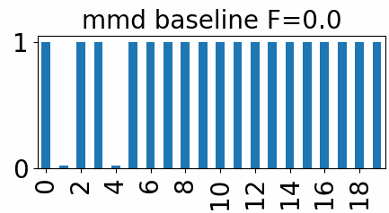
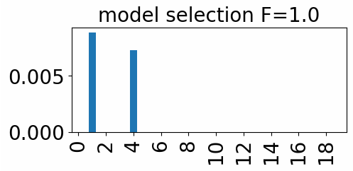
Figure 1: Optimised ARD weights without regularisation (Left) and with regularisation (Right). Here, $S=\{1,4\}$ are the true variables for distinguishing $P$ and $Q$, and $U=\{0,2,3,5,\dots,19\}$ are the redundant variables with zero-variance marginal distributions. Without regularisation, the redundant variables’ ARD weights do not change from their initial value $1$, and bury the weights of the informative variables. With regularisation, these redundant variables are successfully eliminated. The details of the setting are described in Section 5.2 (“Redundant Dirac”).

Regularisation works in variable selection by penalising large weights associated with redundant variables. For example, consider Example 1, where, for the $d$-th variable with $d\in\{1,\dots,D\}$, $P$ and $Q$ have the identical marginal distribution $P_{d}=Q_{d}=\delta_{\xi}$ that is the Dirac distribution at $\xi\in\mathbb{R}$ (say $\xi=1.43)$. Then, for i.i.d. sample vectors ${\bf X}=\{X^{1},\dots,X^{n}\}\subset\mathbb{R}^{D}$ from $P$ and those ${\bf Y}=\{Y^{1},\dots,Y^{m}\}\subset\mathbb{R}^{D}$ from $Q$, their values for the $d$-th variable are all identical to $\xi$: $X_{d}^{1}=\cdots=X_{d}^{n}=Y_{d}^{1}=\cdots=Y_{d}^{m}=\xi$. Therefore the $d$-th variable is redundant for distinguishing $P$ and $Q$. However, as we have $a_{d}^{2}(X_{d}^{i}-X_{d}^{j})^{2}=0$, $a_{d}^{2}(Y_{d}^{i}-Y_{d}^{j})^{2}=0$, $a_{d}^{2}(X_{d}^{i}-Y_{d}^{j})^{2}=0$ for all possible $i$ and $j$, the value of the ARD weight $a_{d}$ does not affect the ARD kernel (7) and thus the objective function (5). Therefore, without regularisation, the maximisation of the objective (5) (or the minimisation of (10) with $\lambda=0$) does not make the ARD weight $a_{d}$ small. Regularisation can fix this issue by penalising non-zero weights associated with such redundant variables. Figure 1 demonstrates how regularisation works.

The question is how to set the regularisation parameter $\lambda$ in (10). If $\lambda$ is too large, most optimised ARD weights may become zero, leading to false negatives. If $\lambda$ is too small, the optimised ARD weights associated with redundant variables may not become zero, leading to false positives (See Appendix E for numerical experiments). Our main methodological contributions are two approaches to the regularisation parameter selection, as described in Sections 4.3 and 4.4.

4.2.1 Variable Selection using the Optimised Weights

As preliminaries to Sections 4.3 and 4.4, we explain how to select variables using the optimised ARD weights $a^{*}=(a^{*}_{1},\dots,a^{*}_{D})$, the solution of (10). One way is to set a threshold $\pi_{\rm thr}\geq 0$ and select variables whose weights are above the threshold: $\hat{S}:=\{d\in\{1,\dots,D\}\mid a^{*}_{d}>\pi_{\rm thr}\}$. The question is how to set the threshold. Our preliminary experiments revealed that the use of a fixed threshold, such as $\pi_{\rm thr}=0$ and $\pi_{\rm thr}=0.1$, does not work well. The reason is that the range of the ARD weights changes drastically depending on the given dataset. For example, the maximum and minimum of the ARD weights can be $10^{-3}$ and $10^{-7}$, respectively, for one dataset, while they can be $10^{2}$ and $10^{-1}$ for another dataset. In either case, however, the ARD weights distribution indicates each variable’s relative importance.

Consequently, we use the following data-driven method for determining the threshold $\pi_{\rm thr}$ based on the histogram of optimised ARD weights. The idea is to set the threshold as the smallest local minimum in the histogram. For instance, if $D=5$, $a^{*}_{1}=0.01$, $a^{*}_{2}=0.02$, $a^{*}_{3}=0.02$, $a^{*}_{4}=0.03$, $a^{*}_{5}=0.1$, we set $\pi^{*}_{\rm thr}=0.03$, and the 5th variable is selected as $a^{*}_{5}=0.1>0.03$. Algorithmically, the method first constructs a histogram of the optimised ARD weights (with 100 bins as a default setting). Subsequently, it identifies bins with zero frequency. Among these bins, the one with the smallest value is selected as threshold $\pi_{\rm thr}$.

4.2.2 Setting Candidate Regularisation Parameters

For the methods for selecting the regularisation parameter $\lambda$ described below, one needs to specify the possible range of $\lambda$ and set candidates from this range. We briefly explain how to do this. More details are available in Appendix D.

Let $\lambda_{\rm lower}$ be the lower bound of the range (we set $\lambda_{\rm lower}=0.01$ as a default setting). Let $\hat{S}_{\lambda}$ denote the set of selected variables using the regularisation parameter $\lambda$. We set the upper bound $\lambda_{\rm upper}$ as the smallest $\lambda$ that makes the number of selected variables to be one, i.e., $|\hat{S}_{\lambda}|=1$, or such that any value $\tilde{\lambda}$ larger than $\lambda$ does not change the selected variables, i.e., $\hat{S}_{\lambda}=\hat{S}_{\tilde{\lambda}}$ for any $\tilde{\lambda}>\lambda$. Appendix D describes how to numerically find such $\lambda_{\rm upper}$.

Once the upper bound $\lambda_{\rm upper}$ is found, we set candidate parameters as follows. Let $N_{\lambda}$ be the number of candidate parameters, and let ${\rm step}_{\lambda}=(\lambda_{\rm upper}-\lambda_{\rm lower})/(N_{\lambda}-1)$. Then we define candidate parameters as $\{\lambda_{\rm lower},\lambda_{\rm lower}+{\rm step}_{\lambda},\dots,\lambda_{\rm lower}+{\rm step}_{\lambda}(N_{\lambda}-1),\lambda_{\rm upper}\}$.

4.3 Method 1: Data-driven Regularisation Parameter Selection

We describe a method for selecting the regularisation parameter $\lambda$ in the optimisation problem (10). Below, let $a_{\lambda}\in\mathbb{R}^{D}$ be the (numerical) solution of (10), and $\hat{S}_{\lambda}$ be the selected variables (as done in Section 4.2.1).

We combine two criteria to select the regularisation parameter. One is the value of the objective function (5) evaluated for the optimised ARD weights $a_{\lambda}$ on held-out validation data: we denote this by $\ell_{{\rm val}}(a_{\lambda})$. The other is the P-value of a permutation two-sample test performed on the selected variables $\hat{S}_{\lambda}$. We select $\lambda$ with the highest $\ell_{{\rm val}}(a_{\lambda})$ among candidates whose P-values are less than $0.05$. The concrete procedure is described in Algorithm 1.

4.3.1 Procedure of Algorithm 1

First, we split the data $({\bf X},{\bf Y})$ into training data $({\bf X}_{\rm train},{\bf Y}_{\rm train})$ and validation data $({\bf X}_{\rm val},{\bf Y}_{\rm val})$. Let $\Lambda$ be a set of candidate parameters (see Section 4.2.2). We perform the following for each $\lambda\in\Lambda$ (lines 2-5). Line 2 obtains optimised ARD weights $a_{\lambda}$ by numerically solving (10) using $\lambda$ and $({\bf X}_{\rm train},{\bf Y}_{\rm train})$. Line 3 then evaluates the objective function (5) on $({\bf X}_{\rm val},{\bf Y}_{\rm val})$ using the ARD weights $a_{\lambda}$; let $\ell_{\rm val}(a_{\lambda})$ be this value. Line 4 selects variables $\hat{S}_{\lambda}\subset\{1,\dots,D\}$ using $a_{\lambda}$ as in Section 4.2.1. Line 5 performs a permutation two-sample test (e.g., [34, Chapter 15]) on the validation data ${\bf X}_{\rm val}([:,\hat{S}_{\lambda}])$ and ${\bf Y}_{\rm val}([:,\hat{S}_{\lambda}])$ where only the selected variables $\hat{S}_{\lambda}$ are used (e.g., if ${\bf X}_{\rm val}$ is given as a $n_{\rm val}\times D$ matrix, then ${\bf X}_{\rm val}([:,\hat{S}_{\lambda}])$ is a $n_{\rm val}\times|\hat{S}_{\lambda}|$ matrix); let $0\leq p_{\lambda}\leq 1$ be the resulting P-value. Once the above procedure is applied for all $\lambda\in\Lambda$, line 8 selects $\lambda^{*}$ with maximum $\ell_{\rm val}(a_{\lambda})$ among those with $p_{\lambda}<0.05$, and returns the corresponding variables $\hat{S}_{\lambda}$ as the final selected variables. If there exists no $\lambda\in\Lambda$ with $p_{\lambda}<0.05$, line 10 selects $\lambda^{*}$ with minimal P-value $p_{\lambda}$, and returns the corresponding variables $\hat{S}_{\lambda^{*}}$.

For the permutation test on the selected variables $\hat{S}_{\lambda}$, one can use, in principle, any test statistic for two sample tests applicable to multivariate data. We found in our preliminary analysis that the sliced Wasserstein distance [19] performs well while running faster than re-optimising the ARD weights on the selected variables $\hat{S}_{\lambda}$, so we use the former in our experiments.

4.3.2 Mechanism

We now discuss the mechanism of the proposed approach of using the two criteria. This approach is based on the following ideas:

1. A high $\ell_{\rm val}(a_{\lambda})$ implies that the selected variable $\hat{S}_{\lambda}$ contains many of the true variables $S$;

2. A low $p_{\lambda}$ implies that $\hat{S}_{\lambda}$ does not contain many of the redundant variables $U:=\{1,\dots,D\}\backslash S$.

Point 1) is because the objective function (5) becomes high when the ARD weights $a_{\lambda}$ lead to a high power of the resulting MMD two-sample test. To see point 2), suppose that $D=5$, the ground-truth variables are $S=\{1,3\}$, the redundant ones are $U=\{2,4,5\}$, and the selected variables are $\hat{S}_{\lambda}=\{1,2,3,4,5\}$. As $\hat{S}_{\lambda}$ contains redundant variables $U$, the permutation test using $\hat{S}_{\lambda}$ may fail to distinguish $P$ and $Q$, since $U$ adds “noises” to “signals” $S$. Accordingly, the P-value $p_{\lambda}$ would not become small.

To understand the mechanism better, suppose that the objective value is high, but the P-value is not small. This happens when the selected variables $\hat{S}_{\lambda}$ contain many of the true variables $S$ but also many of the redundant variables $U$. For instance, consider Example 1, where the ARD weights on the redundant variables $U\backslash V$ do not influence the objective value (5). In this case, the objective value can be large, even if the weights of the redundant variables are large so that the redundant variables are selected. Consequently, the P-value would not be small while the objective value is large.

On the other hand, suppose the objective value is not high, but the P-value is small. This happens when the selected variables $\hat{S}_{\lambda}$ contain some of the true variables $S$ but miss some. To see this, suppose again $D=5$, $S=\{1,3\}$, and that both variables $1$ and $3$ have equally different marginal distributions, i.e., $P_{1}$ and $Q_{1}$ are as different as $P_{3}$ and $Q_{3}$. In this setting, assume that the ARD weights $a_{\lambda}=(a_{\lambda,1},\dots,a_{\lambda,5})$ have a large weight only for variable $1$ (e.g., $a_{\lambda}=(1.6,0.1,0.12,0.2,0.3)$), so that only variable $1$ is selected: $\hat{S}_{\lambda}=\{1\}$. As $P_{1}$ and $Q_{1}$ are different, the permutation test using $\hat{S}_{\lambda}=\{1\}$ would lead to a small P-value. However, because the weight for variable $3$ is not large ($a_{\lambda,3}=0.12$), the objective value $\ell_{\rm val}(a_{\lambda})$ would not become as high as alternative ARD weights where both variables $1$ and $3$ have large weights (e.g., $a_{\lambda}=(1.5,0.2,1.4,0.2,0.1)$). Therefore, the P-value is small in this example, but the objective value would not be high.

To summarize, if the objective value $\ell_{\rm val}(a_{\lambda})$ is high and the P-value $p_{\lambda}$ is small, the selected variables $\hat{S}_{\lambda}$ would contain many of the true variables $S$ but do not contain many redundant variables $U$. Algorithm 1 selects such a regularisation parameter $\lambda$.

Algorithm 1 Data-driven Regularisation Parameter Selection

Input: $\Lambda$: a set of candidate regularisation parameters. $({\bf X}_{\rm train},{\bf Y}_{\rm train})$: training data. $({\bf X}_{\rm val},{\bf Y}_{\rm val})$: validation data.

Output: $\hat{S}_{\lambda^{*}}\subset\{1,\dots,D\}$: selected variables with the best regularisation parameter $\lambda^{*}\in\Lambda$.

1:for all $\lambda\in\Lambda$ do

2:     Obtain ARD weights $a_{\lambda}\in\mathbb{R}^{D}$ by numerically solving (10) using $({\bf X}_{\rm train},{\bf Y}_{\rm train})$ and $\lambda$.

3:     Compute $\ell_{\rm val}(a_{\lambda})>0$ by evaluating (5) on $({\bf X}_{\rm val},{\bf Y}_{\rm val})$.

4:     Select variables $\hat{S}_{\lambda}\subset\{1,\dots,D\}$ using $a_{\lambda}$ as in Section 4.2.1.

5:     Compute P-value $0\leq p_{\lambda}\leq 1$ by performing a permutation two-sample test on $({\bf X}_{\rm val}[:,\hat{S}_{\lambda}],{\bf Y}_{\rm val}[:,\hat{S}_{\lambda}])$.

6:end for

7:if there exists $\lambda\in\Lambda$ with $p_{\lambda}<0.05$ then

8:     $\lambda^{*}=\arg\max_{\lambda\in\Lambda}\{\ell_{\rm val}(a_{\lambda})\mid p_{\lambda}<0.05\}$.

9:else

10:     $\lambda^{*}=\arg\min_{\lambda\in\Lambda}p_{\lambda}$.

11:end if

4.4 Method 2: Cross Validation based Aggregation

Rather than selecting variables based on one “best” regularisation parameter, our second method aggregates the outputs of different regularisation parameters. This method extends our first method by applying cross-validation and computing aggregated scores for the individual variables. It draws inspiration from the Stability Selection algorithm in high-dimensional statistics [35]. (See Appendix F for a systematic comparison with other candidate aggregation strategies for Algorithm 2.)

4.4.1 Procedure of Algorithm 2

Algorithm 2 describes the procedure of the method. For each candidate regularisation parameter $\lambda\in\Lambda$, lines 1 to 10 perform the following. Let $K$ be the number of splits in cross-validation (e.g., $K=10$). For each split $i=1,\dots,K$, line 3 randomly splits the data $({\bf X},{\bf Y})$ into training data $({\bf X}_{\rm train}^{i},{\bf Y}_{\rm train}^{i})$ and validation data $({\bf X}_{\rm val}^{i},{\bf Y}_{\rm val}^{i})$ by the ratio $\rho_{\rm train}$: $1-\rho_{\rm train}$, where $0<\rho_{\rm train}<1$. We set $\rho_{\rm train}=0.5$ as a default value. Lines 4 to 7 perform lines 2 to 5 of Algorithm 1 using $({\bf X}_{\rm train}^{i},{\bf Y}_{\rm train}^{i})$ and $({\bf X}_{\rm val}^{i},{\bf Y}_{\rm val}^{i})$; let $a_{\lambda}^{i}\in\mathbb{R}^{D}$ be the ARD weights, $\hat{S}_{\lambda}^{i}\subset\{1,\dots,D\}$ be the selected variables, $\ell_{\rm val}(a_{\lambda}^{i})$ be the objective value, $0\leq p^{i}_{\lambda}\leq 1$ be the P-value. (See Section 4.3 for the explanation.) Line 8 normalises the ARD weights $a_{\lambda}^{i}=(a_{\lambda,1}^{i},\dots,a_{\lambda,D}^{i})$ by dividing them by the largest weight $\max_{d\in\{1,\dots,D\}}a_{\lambda,d}^{i}$ so that the largest weight of the normalised ones $\tilde{a}_{\lambda}^{i}=(\tilde{a}_{\lambda,1}^{i},\dots,\tilde{a}_{\lambda,D}^{i})$ becomes $1$, i.e., $\max_{d\in\{1,\dots,D\}}\tilde{a}_{\lambda,d}^{i}=1$. This normalisation is needed for the aggregation performed later.

Line 10 computes the $D$-dimensional score vector

$$\hat{\Pi}_{\lambda}:=\frac{1}{K}\sum_{i=1}^{K}I(p_{\lambda}^{i}<0.05)\ell_{\rm val}(a_{\lambda}^{i})\tilde{a}_{\lambda}^{i}\in\mathbb{R}^{D},$$

where $I(p_{\lambda}^{i}<0.05)=1$ if $p_{\lambda}^{i}<0.05$ and $I(p_{\lambda}^{i}<0.05)=0$ if $p_{\lambda}^{i}\geq 0.05$. This vector is the average, over the $K$ splits $i=1,\dots,K$, of the normalised ARD weight vector $\tilde{a}_{\lambda}^{i}$ multiplied by the objective value $\ell_{\rm val}(a_{\lambda}^{i})$ such that the P-value $p_{\lambda}$ is smaller than $0.05$. Line 12 computes the average, over candidate regularisation parameters $\lambda\in\Lambda$, of the score vector $\hat{\Pi}_{\lambda}$ to obtain the aggregated score vector

$$\hat{\Pi}:=\frac{1}{|\Lambda|}\sum_{\lambda\in\Lambda}\hat{\Pi}_{\lambda}\in\mathbb{R}^{D}.$$

Lastly, line 13 selects variables based on the aggregated score $\hat{\Pi}$.

4.4.2 Mechanism

To simplify the explanation, suppose $K=1$, in which case the data $({\bf X},{\bf Y})$ are split into training data $({\bf X}_{\rm train},{\bf Y}_{\rm train})$ and validation data $({\bf X}_{\rm val},{\bf Y}_{\rm val})$ only once as in Algorithm 1. As $K=1$, we do not write the superscript $i$ here. The final score vector $\hat{\Pi}$ in Algorithm 2 is then

$$\hat{\Pi}=\frac{1}{|\Lambda|}\sum_{\lambda\in\Lambda}I(p_{\lambda}<0.05)\ell_{\rm val}(a_{\lambda})\tilde{a}_{\lambda}\in\mathbb{R}^{D}.$$ (11)

This score vector is the weighted average, over different regularisation parameters $\lambda\in\Lambda$, of the normalised ARD weight vector $\tilde{a}_{\lambda}\in\mathbb{R}^{D}$ weighted by the objective value $\ell_{\rm val}(a_{\lambda})$, such that the P-value $p_{\lambda}$ is less than $0.05$.

As discussed in Section 4.3, a large P-value suggests that the selected variables $\hat{S}_{\lambda}$ contain many redundant variables. Therefore, the indicator function $I(p_{\lambda}<0.05)$, which becomes $0$ if $p_{\lambda}\geq 0.05$, effectively excludes such $\lambda$ leading to the selection of redundant variables from the score vector (11). In the score vector (11), a higher contribution is made by the normalised ARD weights $\tilde{a}_{\lambda}\in\mathbb{R}^{D}$ with a higher objective value $\ell_{\rm val}(a_{\lambda})$.

For example, suppose that $D=5$, $\Lambda=\{0.01,0.1,1.0\}$, and

$$\tilde{a}_{0.01}=(0.9,0.8,1.0,0.7,0.6),\quad\ell_{\rm val}(a_{0.01})=12.8,\quad p_{0.01}=0.4$$

$$\tilde{a}_{0.1}=(0.5,0.4,1.0,0.02,0.01),\quad\ell_{\rm val}(a_{0.1})=7.4,\quad p_{0.1}=0.01$$

$$\tilde{a}_{1.0}=(0.2,0.1,1.0,0.0,0.0),\quad\ell_{\rm val}(a_{1.0})=3.1,\quad p_{1.0}=0.01.$$

Then, even if the objective value $\ell_{\rm val}(a_{0.01})=12.8$ for $\lambda=0.01$ is the highest, the normalised ARD weights $\tilde{a}_{0.01}$ for $\lambda=0.01$ do not contribute to the score vector (11), because the P-value $p_{0.01}=0.4$ is higher than the threshold $0.05$. As $p_{0.1}<0.05$ and $p_{1.0}<0.05$, the normalised ARD weight vectors $\tilde{a}_{0.1}$ and $\tilde{a}_{1.0}$ contribute to the score vector (11). Because the objective value $\ell_{\rm val}(a_{0.1})=7.4$ for $\lambda=0.1$ is higher than $\ell_{\rm val}(a_{1.0})=3.1$ for $\lambda=1.0$, the normalised ARD weights $\tilde{a}_{0.1}$ for $\lambda=0.1$ contribute to the score vector more significantly than the normalised ARD weights $\tilde{a}_{1.0}$ for $\lambda=1.0$. The score vector then becomes $\hat{\Pi}=(4.32,3.27,10.5,0.148,0.074)$. Applying the procedure in Section 4.2.1 to $\hat{\Pi}$, the first three variables would be selected: $\hat{S}=\{1,2,3\}$.

A critical difference between the algorithms is that Algorithm 1 selects one “best” regularisation parameter $\lambda$ maximizing the objective value $\ell_{\rm val}(a_{\lambda})$ among candidates with small P-values, while Algorithm 2 aggregates the scores (as given by the normalised ARD weights) from different regularisation parameters (with small P-values) by weighting with the objective values. In the above example, Algorithm 1 would only use the ARD weights $a_{\lambda}$ with $\lambda=0.1$, while Algorithm 2 uses the (normalised) ARD weights $\tilde{a}_{\lambda}$ for $\lambda=0.1$ and $\lambda=1.0$ with their associated objective values. Therefore, Algorithm 2 exploits more information and thus could perform more stable variable selection. Another difference is that Algorithm 2 uses cross-validation, which can effectively improve the stability of the score vector when the sample sizes $n,m$ are small. On the other hand, Algorithm 1 is faster to compute and thus more advantageous for large sample sizes.

Algorithm 2 Cross Validation based Aggregation

Input: $\Lambda$: a set of candidate regularisation parameters. ${\bf X}=\{X^{1},\dots,X^{n}\}\subset\mathbb{R}^{D}$ and ${\bf Y}=\{Y^{1},...,Y^{m}\}\subset\mathbb{R}^{D}$: data. $K$: the number of cross-validation splits. $\rho_{\rm train}\in(0,1)$: training-validation splitting ratio (default value: $0.5$).

Output: $\hat{S}\subset\{1,\dots,D\}$: selected variables.

1:for all $\lambda\in\Lambda$ do

2:     for all $i\in\{1,...,K\}$ do

3:         Randomly split $({\bf X},{\bf Y})$ into $({\bf X}_{\rm train}^{i},{\bf Y}_{\rm train}^{i})$ and $({\bf X}_{\rm val}^{i},{\bf Y}_{\rm val}^{i})$ by the ratio $\rho_{\rm train}:1-\rho_{\rm train}$.

4:         Obtain ARD weights $a_{\lambda}^{i}\in\mathbb{R}^{D}$ by optimising (10) using $({\bf X}_{\rm train}^{i},{\bf Y}_{\rm train}^{i})$ and $\lambda$.

5:         Compute $\ell_{\rm val}(a_{\lambda}^{i})>0$ by evaluating (5) on $({\bf X}_{\rm val}^{i},{\bf Y}_{\rm val}^{i})$.

6:         Select variables $\hat{S}_{\lambda}^{i}\subset\{1,\dots,D\}$ using $a_{\lambda}^{i}$ as in Section 4.2.1.

7:         Compute P-value $0\leq p_{\lambda}^{i}\leq 1$ by performing a permutation two-sample test on $({\bf X}_{\rm val}[:,\hat{S}_{\lambda}^{i}],{\bf Y}_{\rm val}[:,\hat{S}_{\lambda}^{i}])$.

8:         Compute $\tilde{a}_{\lambda}^{i}:=a_{\lambda}^{i}/\left(\max_{d\in\{1,\dots,D\}}a_{\lambda,d}^{i}\right)\in\mathbb{R}^{D}$

9:     end for

10:     Compute $\hat{\Pi}_{\lambda}:=\frac{1}{K}\sum_{i=1}^{K}I(p_{\lambda}^{i}<0.05)\ell_{\rm val}(a_{\lambda}^{i})\tilde{a}_{\lambda}^{i}\in\mathbb{R}^{D}$.

11:end for

12:Compute $\hat{\Pi}:=\frac{1}{|\Lambda|}\sum_{\lambda\in\Lambda}\hat{\Pi}_{\lambda}\in\mathbb{R}^{D}$.

13:Select variables $\hat{S}\subset\{1,\dots,D\}$ using $\hat{\Pi}$ as in Section 4.2.1.

5 Empirical Assessment

This section describes empirical assessments of the proposed methods. We only report selected results here due to the page limitation; additional results are available in the appendix. Section 5.1 explains common settings for different experiments. Section 5.2 describes experiments with synthetic datasets. Section 5.3 reports experiments using data generated from a traffic simulator.

5.1 Common Settings

We compare the proposed Algorithms 1 and 2 with three baseline methods. The first baseline is the approach by Sutherland [2, Section 5], which we call here mmd-baseline. It optimises the ARD weights by maximising the objective function (5) (or minimising (10) with $\lambda=0$) and performs variable selection using the optimised ARD weights as in Section 4.2.1. The second baseline is the approach by Lim et al. [11], referred to as mskernel-star; see Section 2.2 for its explanation. We use the implementation by the authors. This method requires the number of selected variables as a hyper-parameter; we set it to the number of ground-truth variables. The third baseline uses the L1-regularised logistic regression, and we call it regression-baseline. This method performs a classifier two-sample test using L1-regularised linear logistic regression. The learned coefficients of the regression model are used for variable selection as in Section 4.2.1. We tune this method’s regularisation parameter by grid search of its inverse from the range $[-4,4]$ by performing 5-fold cross-validation.

We refer to Algorithms 1 and 2 as model-selection and CV-aggregation, respectively. In addition to these methods, we report the results for mmd-tuning-best-F1, which optimises the regularised objective (10) using the regularisation parameter tuned to maximise the F score (introduced below). In practice, this method cannot be implemented because the F score is unavailable as it requires knowing the ground-truth variables; we show its results to provide the best possible performance of Algorithm 1.

We use the Gaussian ARD kernel (4) for the kernel-based approaches. We set the length-scale parameters $\gamma_{1},\dots,\gamma_{D}$ by the variable-wise median heuristic described in Appendix C. We use the Adam optimiser to optimise (10) for the ARD weights. For its learning rate, we use the ReduceLROnPlateau learning rate scheduler of PyTorch, which starts from 0.01 and adaptively reduces the learning rate based on the changes in objective values. The initial value for each ARD weight is set to $1$. An early-stopping rule triggers if the difference between the maximum and minimum objective values (10) (on both training and validation data) for 100 consecutive epochs is less than 0.001; we set the maximum number of epochs to 99,999. For Algorithms 1 and 2, we obtain candidate $\Lambda$ regularisation parameters by the method described in Section 4.2.2. For Algorithm 2, we set the number of cross-validation splits to $K=10$. To compute the P-values using the sliced Wasserstein distance for Algorithms 1 and 2, we use the POT Python package [36].

5.2 Synthetic Data Experiments

We report experiments on synthetically generated datasets where the ground-truth variables are available for evaluation. We describe only selected results; more can be found in Appendix G. Below, let $\mathbb{N}({\bf\mu},\Sigma)$ be the $D$-dimensional Gaussian distribution with mean vector ${\bf\mu}=(\mu_{1},\dots,\mu_{D})^{\top}\in\mathbb{R}^{D}$ and covariance matrix $\Sigma\in\mathbb{R}^{D\times D}$.

5.2.1 Data Generation Processes and Evaluation Criteria

We generate datasets ${\bf X}=\{X^{1},\dots,X^{n}\}\stackrel{{\scriptstyle i.i.d.}}{{\sim}}P$ and ${\bf Y}=\{Y^{1},\dots,Y^{n}\}\stackrel{{\scriptstyle i.i.d.}}{{\sim}}Q$ as i.i.d. samples from probability distributions $P$ and $Q$ on $\mathbb{R}^{D}$, where $n=200$ and $D=20$ (see Appendix G.2 for experiments with higher $D$). We explain below how to define these probability distributions $P$ and $Q$.

Let $P=\mathcal{N}({\bf 0}_{D},I_{D})$, where ${\bf 0}_{D}:=(0,\dots,0)^{\top}\in\mathbb{R}^{D}$ and $I_{D}\in\mathbb{R}^{D\times D}$ is the identity matrix. We define $Q$ as follows. Let $S\subset\{1,\dots,D\}$ be a set of ground-truth variables with the cardinality $|S|=\lfloor\rho\times D\rfloor$, where $\rho\in(0,1)$. Here, we set $\rho=0.1$, so $|S|=2$ (see Appendix G.1 for experiments with higher $\rho$). We define $Q_{S}$ as a marginal distribution on $\mathbb{R}^{|S|}$ such that $Q_{S}\not=P_{S}$, where $P_{S}=\mathcal{N}({\bf 0}_{|S|},I_{|S|})$ is the marginal distribution of $P$ on $S$. Then we define $Q:=Q_{S}\otimes P_{\{1,\dots,D\}\backslash S}$, where $P_{\{1,\dots,D\}\backslash S}=\mathcal{N}({\bf 0}_{D-|S|},I_{D-|S|})$ is the marginal distribution of $P$ on $\{1,\dots,D\}\backslash S$. More specifically, we consider the following five different ways of defining $Q_{S}$ (and thus $Q$):

1. Shifted means: $Q_{S}=\mathcal{N}({\bf 0.5}_{|S|},I_{|S|})$, where ${\bf 0.5}_{|S|}=(0.5,\dots,0.5)^{|S|}\in\mathbb{R}^{|S|}$.

2. Wider variances: $Q_{S}=\mathcal{N}({\bf 0}_{|S|},1.5I_{|S|})$.

3. Narrower variances: $Q_{S}=\mathcal{N}({\bf 0}_{|S|},0.5I_{|S|})$.

4. Laplace distribution: $Q_{S}=\mathcal{L}({\bf 0}_{|S|},I_{|S|})$ is the Laplace distribution on $\mathbb{R}^{|S|}$ with the same mean ${\bf 0}_{|S|}$ and covariance matrix $I_{|S|}$.

5. Correlated Gaussian: the random vector $(y_{1},\dots,y_{|S|})\sim Q_{S}$ is defined as follows. Generate $y_{1}\sim\mathcal{N}(0,1)$ and set $y_{2}=\cdots=y_{|S|}=y_{1}$.

We also consider the following setting corresponding to that discussed in Sections 4.1 and 4.2.

1. Redundant Dirac: $P_{S}=\mathcal{N}({\bf 0}_{|S|},I_{|S|})$, $Q_{S}=\mathcal{N}({\bf 0.5}_{|S|},I_{|S|})$ and $P_{\{1,\dots,D\}\backslash S}=Q_{\{1,\dots,D\}\backslash S}=\delta_{{\bf 0}_{D-|S|}}$, where $\delta_{{\bf 0}_{D-|S|}}$ is the Dirac distribution at ${\bf 0}_{D-|S|}=(0,\dots,0)^{\top}\in\mathbb{R}^{D-|S|}$.

For each of these settings, we generate datasets ${\bf X}=\{X^{1},\dots,X^{200}\}\stackrel{{\scriptstyle i.i.d.}}{{\sim}}P=P_{S}\otimes P_{\{1,\dots,D\}\backslash S}$ and ${\bf Y}=\{Y^{1},\dots,Y^{200}\}\stackrel{{\scriptstyle i.i.d.}}{{\sim}}Q=Q_{S}\otimes P_{\{1,\dots,D\}\backslash S}$, run each method to select variables $\hat{S}\subset\{1,\dots,D\}$, and evaluate the Recall (Re), Precision (Pr) and the F score w.r.t. the ground-truth variables $S\subset\{1,\dots,D\}$. These evaluation criteria are defined as

$${\rm Pr}=\frac{|\hat{S}\cap S|}{|\hat{S}|},\hskip 8.61108pt{\rm Re}=\frac{|\hat{S}\cap S|}{|S|},\hskip 8.61108ptF=\frac{2\times{\rm Pr}\times{\rm Re}}{{\rm Pr}+{\rm Re}}$$ (12)

The precision is the ratio of the true positives among the selected variables, the recall is the ratio of the true positives among the ground-truth variables, and the F score is their harmonic mean; higher values indicate better variable selection performance. We repeat the above procedure 10 times independently, and compute averages and standard deviations of the criteria.

5.2.2 Results

Figure 2 describes the results. For 1) Shifted means, 2) Wider variances, 3) Narrower variances and 4) Laplace distribution, the three baseline methods (regression-baseline, mskernel-star and mmd-baseline) consistently yield low F scores, indicating the difficulty of variable selection in these settings where the differences between $P$ and $Q$ are subtle. These low F scores are due to many false positives, as evidenced by the low precisions and high recalls.

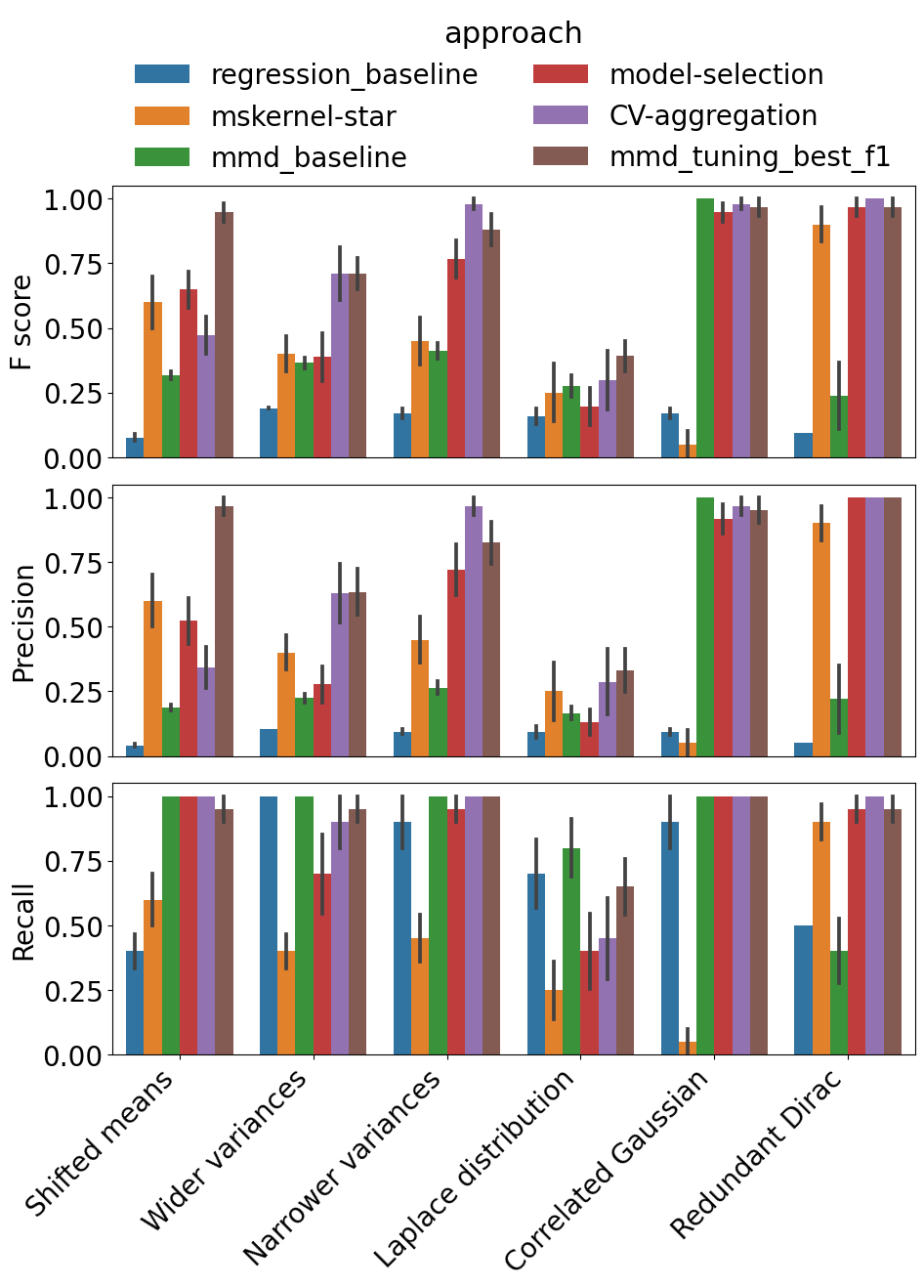
Figure 2: Results of the synthetic data experiments in Section 5.2. Top, middle and bottom plots show the F score, precision and recall, respectively. The groups correspond to the six settings. Each bar reports mean and standard deviation over 10 experiment executions.

For 5) Correlated Gaussian, mskernel-star fails to detect any correct variables, resulting in zero precision and zero recall. This is because mskernel-star only examines the differences between univariate marginal distributions (i.e., $P_{d}$ v.s. $Q_{d}$ for each $d=1\dots,D$); however, the univariate marginals distributions for 5) are all the same; the differences appear only in the correlation structures of $P$ and $Q$, which cannot be detected by mskernel-star.

For 6) Redundant Dirac, mmd-baseline exhibits a significant drop in recall compared with the other settings. This is because in 6) the regularisation is necessary to eliminate the ARD weights of redundant variables; Figure 1 shows a visualization of the issue.

Algorithms 1 and 2 (model-selection and CV-aggregation) yield higher F scores than the three baselines for most settings, indicating that the proposed methods address the above challenges. CV-aggregation performs better than or comparably with model-selection. Notably, CV-aggregation even outperforms mmd-tuning-best-f1 for some settings. Recall that mmd-tuning-best-f1 is not implementable in practice and is meant to provide the best possible F score of Algorithm 1.

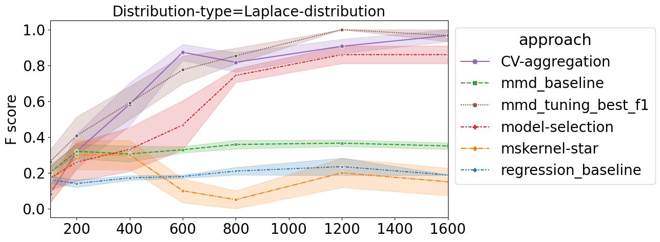
Figure 3: F scores for different sample sizes in the Laplace distribution setting in Section 5.2. The horizontal axis indicates sample size $n$. For each sample size and each method, the confidence interval shows the standard deviation of the F scores over 10 experiments.

Figure 3 describes how the F score of each method changes as the sample size $n$ increases for the 4) Laplace distribution setting. The F scores of model-selection and CV-aggregation increase with higher sample size, suggesting that the methods identify ground-truth variables with subtle distributional changes with large enough samples. On the other hand, the F scores of the baseline methods do not improve for larger sample sizes and they are significantly lower than model-selection and CV-aggregation. CV-aggregation achieves a high F score of $0.87$ with sample size $600$, while model-selection requires sample size $1200$ to reach a similar F score. This suggests that CV-aggregation makes a more effective use of data than model-selection as remarked in Section 4.4.

5.3 Exploratory Data Analysis of Traffic Simulation Data

We demonstrate how the proposed methods can be applied to exploratory data analysis (see Appendix A for another demonstration using image datasets). As an illustrative example, suppose we are interested in analysing datasets obtained from a city-scale traffic system. The form of data is a matrix $X\in\mathbb{R}^{D_{\rm sensor}\times D_{\rm time}}$, where $D_{\rm sensor}$ is the number of sensors located in the road network and $D_{\rm time}$ is the number of time intervals. The $(d,t)$-th entry $X_{d,t}$ of $X$ represents the number of vehicles detected by the $d$-th sensor during the $t$-th time interval. For example, in our experiments below, we have $D_{\rm sensor}=64$ sensors and $D_{\rm time}=12$ time intervals, where each time interval is for 5 minutes; thus, one matrix $X$ records the traffic flows observed by the $64$ sensors for the duration of $60=12\times 5$ minutes.

Suppose now that we have two sets of such data matrices ${\bf X}=\{X^{1},\dots,X^{n}\}\subset\mathbb{R}^{D_{\rm sensor}\times D_{\rm time}}$ and ${\bf Y}=\{Y^{1},\dots,Y^{m}\}\subset\mathbb{R}^{D_{\rm sensor}\times D_{\rm time}}$ from two different settings. For example, one dataset ${\bf X}$ may be generated from a traffic simulator modelling the rush hours (8 pm - 9 pm) of the city, and the other dataset ${\bf Y}$ may consist of real observations from the city’s rush hours. By analysing how the two datasets ${\bf X}$ and ${\bf Y}$ differ, one can understand which aspects the simulator fails to model the city’s real traffic system; such insights can be used for improving the simulator.

We demonstrate how our CV-aggregation (Algorithm 2) can be used to analyse such datasets. To this end, we treat each data matrix ${\bf X}\in\mathbb{R}^{D_{\rm sensor}\times D_{\rm time}}$ as a $D=D_{\rm sensor}\times D_{\rm time}$-dimensional vector. Each variable $d\in\{1,\dots,D\}$ corresponds to one specific pair of a sensor and a time interval. Therefore, ${\bf X}=\{X^{1},\dots,X^{n}\}$ and ${\bf Y}=\{Y^{1},\dots,Y^{m}\}$ can be regarded as two sets of $D$-dimensional vectors, and CV-aggregation can be used for selecting variables (= sensor-time pairs) where traffic flows in the two datasets differ significantly.

Experiment Setup

We briefly describe the data generation process. For details, see Appendix H. We generate both datasets ${\bf X}$ and ${\bf Y}$ from a microscopic stochastic traffic simulator but from two different scenarios. We define a grid-like road network consisting of 8 intersections and $D_{\rm sensor}=64$ sensors, and define one scenario where vehicles travel to their destinations for the duration of 60 minutes; we call it scenario $P$. We define another scenario, which we call scenario $Q$, as a perturbed version of scenario $P$ where two specific roads are blocked for the first 40 minutes. We define $D_{\rm time}=12$ time intervals, each 5 minutes. As mentioned, one simulation yields a matrix of the form $X\in\mathbb{R}^{D_{\rm sensor}\times D_{\rm time}}$, where the $(d,t)$-th element $X_{d,t}$ of the matrix $X$ is the number of vehicles detected by the $d$-th sensor during the $t$-th time interval ($d=1,\dots,D_{\rm sensor}$ and $t=1,\dots,D_{\rm time}$). We generate ${\bf X}=\{X^{1},\dots,X^{n}\}\subset\mathbb{R}^{D_{\rm sensor}\times D_{\rm time}}$ from scenario $P$ with $n$ random seeds, and ${\bf Y}=\{Y^{1},\dots,Y^{n}\}\subset\mathbb{R}^{D_{\rm sensor}\times D_{\rm time}}$ from scenario $Q$ with $n$ random seeds, with $n=400$.

We use CV-aggregation with the same configuration as Section 5.1 with one modification on the choice of the length-scale parameters $\gamma_{1},\dots,\gamma_{D}$ with $D=D_{\rm sensor}\times D_{\rm time}$. A preliminary analysis showed that the variable-wise median heuristic in Appendix C.1 yields zeros for some of $\gamma_{1},\dots,\gamma_{D}$ in this setting (which is problematic, as the length-scales should be positive by definition). The reason is each data matrix in the datasets ${\bf X}$ and ${\bf Y}$ contain many entries whose values are zero; these entries are sensor-time pairs in which no vehicle was detected. We therefore use the variable-wise mean instead of median for setting $\gamma_{1},\dots,\gamma_{D}$ here.

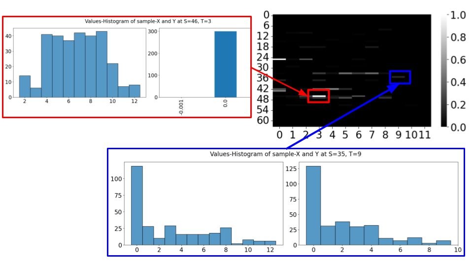
Figure 4: The right bottom heat map describes the score matrix $\hat{\Pi}\in\mathbb{R}^{D_{\rm sensor}\times D_{\rm time}}$, which is normalized so that the highest value is $1$. The vertical axis indexes $D_{\rm sensor}=64$ sensors, and the horizontal axis indexes the $D_{\rm time}=12$ time intervals. The sensor-time pair in red has the highest score, and the sensor-time pair in blue has the lowest score among the selected variables. For each sensor-time pair, the two histograms represent the empirical distributions of the vehicle counts in the datasets ${\bf X}=\{X^{1},\dots,X^{400}\}\subset\mathbb{R}^{D_{\rm sensor}\times D_{\rm time}}$ (left) and ${\bf Y}=\{Y^{1},\dots,Y^{400}\}\subset\mathbb{R}^{D_{\rm sensor}\times D_{\rm time}}$ (right) at this sensor-time pair. Note that the horizontal axis of each histogram is the number of vehicles observed in the time-interval of 5 minutes (= 300 seconds) per second; thus, for example, the value $0.02$ indicates that the $0.02\times 300=6$ vehicles were observed in the time interval.

Analysis Demonstration

Without any knowledge about the fact that two roads are blocked in the scenario $Q$ dataset ${\bf Y}$, we apply CV-aggregation to the two datasets ${\bf X}$ and ${\bf Y}$ and see whether it can identify sensor-time pairs where the traffic flows are affected by this road blocking. (Appendix H contains the results of other methods.) Note, however, that it is not straightforward to define the “ground truth” for this experiment, as the blocking of the roads would affect not only the traffic flows of the blocked roads during the 40 minutes of the road blocking, but also the traffic flows of the surrounding roads and subsequent periods. Therefore, we demonstrate explanatory data analysis using the proposed method.

As a result of applying CV-aggregation, we obtained 22 variables (= sensor-time pairs) selected from $D=64\times 12=768$ variables, together with the score matrix $\Pi\in\mathbb{R}^{D_{\rm sensor}\times D_{\rm time}}$ in Algorithm 2. Figure 4 describes $\hat{\Pi}$ as a heat map, along with the sensor-time pairs with the highest (highlighted in red) and lowest scores (highlighted in blue) among the selected variables. The two histograms for each sensor-time pair represent the empirical distributions of the 400 vehicle counts in the two datasets ${\bf X}=\{X^{1},\dots,X^{400}\}$ and ${\bf Y}=\{Y^{1},\dots,Y^{400}\}$ at this sensor-time pair.

At the sensor-time pair with the highest score (red), the traffic patterns in the two datasets differ significantly. Indeed, the left histogram indicates active traffic flows in the dataset ${\bf X}$, while the right histogram shows no traffic flow in the dataset ${\bf Y}$ at this sensor-time pair. In an actual explanatory analysis, one could hypothesise that there is a road blocking around this sensor and investigate the neighbouring sensors and time periods. The sensor-time pair associated with the lowest score among the selected variables (blue) also provides insights into the difference between the two datasets ${\bf X}$ and ${\bf Y}$. While the two histograms look similar, there are subtle differences in the probability masses in the lower and upper limits of the histograms. This time interval is around the end of the road blocking, and thus this sensor-time pair provides a hint about the end time and final effects of the unknown incident (= road blocking) in the scenario $Q$.

6 Conclusion and Future Directions

We have presented novel approaches to variable selection in MMD to enable interpretable distribution comparison. The proposed methods have many potential applications, as the comparison of datasets is a fundamental task appearing in many problems of machine learning and pattern recognition. For example, domain adaptation, which is to adapt a trained learning machine to a new test domain and is an active area of research, requires analysing how training and test data distributions differ. The proposed methods enable the identification of variables where domain shifts occur, and the information on such selected variables could be used in a domain adaptation method. Other critical applications include model validation and calibration of a generative model (or a simulator), where one needs to assess how the real and generated datasets differ; and causal inference, where one is interested in how the outcome distributions (e.g. patients’ health outcomes) under different treatments (e.g., medicines) differ.

One potential future direction is to make the proposed methods scalable to large datasets. Since evaluating the objective function (10) requires quadratic complexity to the sample size, it can be slow when the sample size is large. A straightforward extension is to adapt the linear MMD estimator [17] (see the appendix for preliminary experiments) or Fourier-feature type approximations [23] in the proposed methods. Another key direction is developing a statistical theory to better understand the proposed methods, such as the consistency of the proposed methods for estimating the ground-truth variables $S$ in Definition 1. To this end, one needs to analyse the asymptotic behaviour of the solution of the regularised objective (10), but this may be challenging because of the non-concavity of the ratio objective (5) with respect to the ARD weights. We leave this analysis for future work.

Acknowledgements

MK has been supported by the French Government through the 3IA Cote d’Azur Investment in the Future Project managed by the National Research Agency (ANR) with the reference number ANR-19-P3IA-0002. We acknowledge support from Huawei Research and Development.

Kensuke Mitsuzawa has been a PhD candidate at EURECOM, France, since 2021. He obtained his BA from the Department of Foreign Studies of Osaka University (Japan) and his M.E. in Computer Science: Information Science at Nara Institute of Science and Technology (Japan) in 2012. His research is focused on interpretable two-sample testing and parameter estimation for simulators.

Motonobu Kanagawa has been an Assistant Professor in the Data Science Department at EURECOM, France, since 2019. He has also been a Chair at 3IA Côte d’Azur, a French national institute on AI research, since 2021. Previously, he was a research scientist at the Max Planck Institute for Intelligent Systems and the University of Tuebingen in Germany from 2017 to 2019. Before this, he was a postdoc (2016-2017) and a PhD student (2013-2016) at the Institute of Statistical Mathematics, Japan.

Stefano Bortoli received a PhD in Computer Science at the University of Trento (Italy) in 2013. Currently, is Principal Research Engineer and Team Manager at Huawei Munich Research Center, leading a team in the investigation of research problems in the area of Smart City, with particular focus on Traffic Optimization, Traffic Simulation and in general high-performance and scalable City Simulation. Has a background in research and development of technologies for big data and stream processing frameworks that are currently part of real-world cloud services.

Margherita Grossi is a Principal Research Engineer for applied AI and ML at Huawei Munich Research Center. Previously, she was a Senior and Lead Data Scientist at Telefónica Germany (2017-2020) and a Data Scientist at the German Aerospace Center (2011-2017). She holds a PhD from the Max Planck Institute for Astrophysics and Ludwig Maximilian University of Munich, where she investigated cosmological models with HPC simulations as a graduate student and postdoc researcher (2006-2011). Photograph is not available at time of publication.

Paolo Papotti is an Associate Professor at EURECOM, France, since 2017. He got his PhD from Roma Tre University (Italy) in 2007 and had research positions at the Qatar Computing Research Institute (Qatar) and Arizona State University (USA). His research is focused on data integration and information quality. He has authored more than 140 publications, and his work has been recognized with two “Best of the Conference” citations (SIGMOD 2009, VLDB 2016), three best demo award (SIGMOD 2015, DBA 2020, SIGMOD 2022), and two Google Faculty Research Award (2016, 2020).

Supplementary Materials

The supplementary materials are organised as follows.

• Appendix A demonstrates the application of the proposed methods using face images of cats and dogs.

• Appendix B provides the proofs of theoretical results.

• Appendix C explains methods for selecting length-scale parameters $\gamma_{1},\dots,\gamma_{D}$ in the ARD kernel.

• Appendix D describes how to obtain a set of candidate regularisation parameters.

• Appendix E investigates the effects of the regularisation parameter on the variable selection performance.

• Appendix F compares different candidate aggregation strategies for CV-aggregation (Algorithm 2).

• Appendix G reports additional results for the experiments in Section 5.2.

• Appendix H explains the details of the experiments in Section 5.3 and reports additional results.

• Appendix I performs a preliminary experiment using a linear MMD estimator.

• Appendix J makes a comparison with an alternative regularised objective function where the MMD estimate replaces the ratio objective.

Appendix A Demonstration: Analysing Cat and Dog Images

We demonstrate the application of the proposed approaches in analysing image datasets. We use a subset of the AFHQ dataset [37] consisting of high-resolution images of cats’ and dogs’ faces, as described in Figure 5. The aim here is to select variables (= pixel coordinates) that indicate differences between cats’ and dogs’ faces.

As preprocessing, we downscale the resolution of each image data to $64\times 64$ pixels, resulting in a total of $4,096$ dimensions. We convert each pixel’s RGB values into a greyscale value ranging from $0$ to $255$. For our experiments, we randomly selected 1,000 images from the AFHQ dataset containing 5,000 images. Here, we optimise the ARD weights using the Adam optimiser using 100 batches in each iteration. See Section 5.1 for other details.

Figure 7 describes the score matrices obtained with mmd-baseline, model-selection and CV-aggregation. As CV-aggregation performs the best in our other assessments, we examine the variables selected by CV-aggregation. Figure 6 shows some cats’ and dogs’ face images on which the selected variables (pixel positions) are highlighted as yellow dots.

By examining Figure 6, we can observe that the selected variables capture discrepancies between cats’ and dogs’ faces in mainly four areas: 1) the shape of the left eye, 2) the shape of the right eye, 3) the shape from the nose to the chin, and 4) the position of the forehead. Regarding the eyes’ shapes, cats’ eyes are typically wide and oval-shaped, while dogs’ eyes tend to be elongated ellipse-shaped. In addition to the shapes/positions of parts of a face, colour depths (i.e., greyscale values from $0$ to $255$) may also contribute to the discrepancies between cats’ and dogs’ faces. For example, cats’ eyes tend to be transparent (resembling glass), while dog’s eyes are darker. Differences between cats and dogs in the shape from the nose to the chin are also noticeable. A cat’s nose is small and pointy, and its chin shapes a gentle curve, while a dog has a larger and rounded black-blob-shaped nose and a more acute chin.

For further analysis, we compare the histograms of greyscale values in the datasets at specific pixel positions: the pixel at the 27th row and the 21st column (located on the upper left of the left eye) and at the pixel at the 47th row and the 36th column (located on the right side of the nose). These pixels have the highest and second scores given by CV-aggregation. Figure 8 shows the histograms at these pixels. Examining the histogram of the pixel at the 27th row and the 21st column, we observe that dog images have higher frequencies in low greyscale values than cat images. Since low greyscale values indicate darker colours, this may indicate the presence of dark iris colours in dogs’ eyes. Similarly, for the pixel at the 47th row and the 36th column, dog images have higher frequencies in low greyscale values (dark colours). This pixel is often associated with a part of the nose, implying differences in the nose shapes and colours between cats and dogs.

(a) flickr_cat_000060.jpg	(b) pixabay_cat_000588.jpg
(c) flickr_dog_000039.jpg	(d) pixabay_dog_000969.jpg

Figure 5: Examples of cats’ and dogs’ face images from the AFHQ dataset. The caption of each image indicates the file name in the dataset.

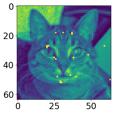
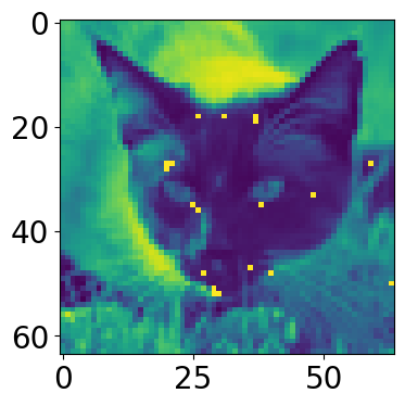
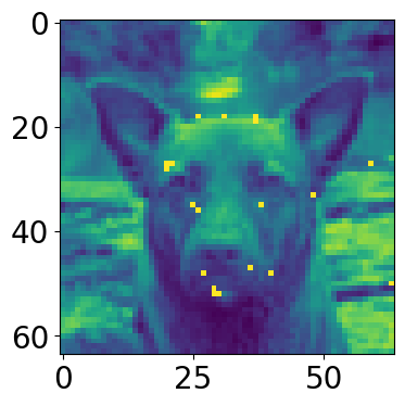
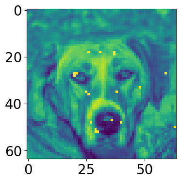
Figure 6: Example images of cats’ and dogs’ faces after preprocessing (down-scaled to $64\times 64$ pixels, with colours transformed to greyscale values), corresponding to Figure 5, where the pixel positions (=variables) selected by CV-aggregation are highlighted in yellow.

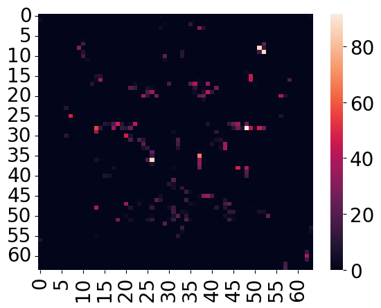
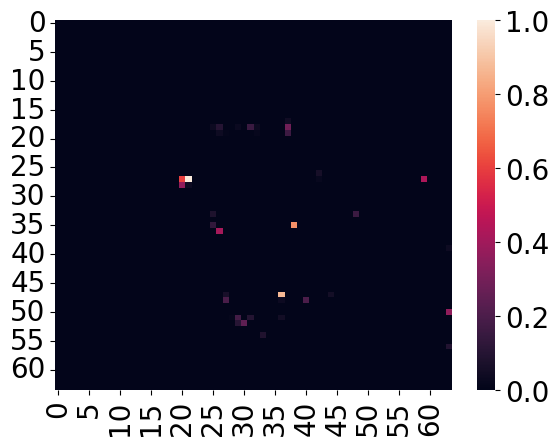
(a) Optimised ARD weights obtained by mmd-baseline	(b) Optimised ARD weights obtained by model-selection
(c) The score matrix obtained from CV-aggregation

Figure 7: Score matrices obtained with (a) mmd-baseline, (b) model-selection and (c) CV-aggregation.

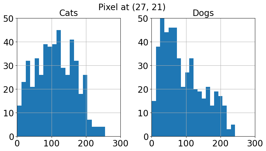
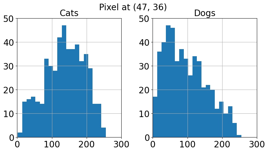
Figure 8: Histograms of greyscale values for the pixel at the 27th row and the 21st column (left two histograms) and those at the 47th row and 36th row (right two histograms).

Appendix B Proofs of Theoretical Results

B.1 Proof of Proposition 1

Proof.

We first prove that the uniqueness of $S$ satisfying the conditions in Definition 1. To this end, suppose that there exist two subsets $S_{1}\subset[D]$ and $S_{2}\subset[D]$ satisfying the conditions in Definition 1. Then we shall prove that $S_{0}=S_{1}\cup S_{2}$ satisfies the conditions in Definition 1, which implies $S_{1}=S_{2}$ (otherwise $S_{1}\varsubsetneq S_{0}$ and $S_{2}\varsubsetneq S_{0}$, which contradicts Definition 1).

To prove that $S_{0}$ satisfies Definition 1, suppose that $S_{0}$ does not satisfy it, i.e., there exists a non-empty subset $U_{0}\subset S_{0}$ such that $P_{S_{0}}=P_{U_{0}}\otimes P_{S_{0}\backslash U_{0}}$ , $Q_{S_{0}}=Q_{U_{0}}\otimes Q_{S_{0}\backslash U_{0}}$ and $P_{U_{0}}=Q_{U_{0}}$. Let $U_{1}:=U_{0}\cap S_{1}$ and $U_{2}:=U_{0}\cap S_{2}$. We either have $U_{1}\not=\phi$ or $U_{2}\not=\phi$, because

$$\phi \not=U_{0}\cap S_{0}=U_{0}\cap(S_{1}\cup S_{2})$$

$$=(U_{0}\cap S_{1})\cup(U_{0}\cap S_{2})=U_{1}\cup U_{2}.$$

Without loss of generality, suppose $U_{1}\not=\phi$. For $A\subset[D]$, let $A^{c}:=[D]\backslash A$. Note that

$$U_{0}\backslash(U_{0}\cap(S_{0}\backslash S_{1}))=U_{0}\cap(U_{0}\cap(S_{0}\backslash S_{1}))^{c}$$

$$=U_{0}\cap(U_{0}^{c}\cup(S_{0}\backslash S_{1})^{c})=U_{0}\cap(S_{0}\backslash S_{1})^{c}$$

$$=U_{0}\cap(S_{0}\cap S_{1}^{c})^{c}=U_{0}\cap(S_{0}^{c}\cup S_{1})=U_{0}\cap S_{1}=U_{1}\not=\phi.$$

Similarly, we have

$$(S_{0}\backslash U_{0})\backslash[(S_{0}\backslash U_{0})\cap(S_{0}\backslash S_{1})]$$

$$=(S_{0}\backslash U_{0})\cap[(S_{0}\backslash U_{0})\cap(S_{0}\backslash S_{1})]^{c}$$

$$=(S_{0}\backslash U_{0})\cap[(S_{0}\backslash U_{0})^{c}\cup(S_{0}\backslash S_{1})^{c}]=(S_{0}\backslash U_{0})\cap(S_{0}\backslash S_{1})^{c}$$

$$=(S_{0}\cap U_{0}^{c})\cap(S_{0}\cap S_{1}^{c})^{c}=(S_{0}\cap U_{0}^{c})\cap(S_{0}^{c}\cup S_{1})$$

$$=U_{0}^{c}\cap[(S_{0}\cap S_{0}^{c})\cup(S_{0}\cap S_{1})]$$

$$=U_{0}^{c}\cap S_{1}=S_{1}\backslash U_{0}=S_{1}\backslash U_{1}.$$

Therefore,

$$P_{S_{1}}(x_{S_{1}})=\int P_{S_{0}}(x)dx_{S_{0}\backslash S_{1}}$$

$$=\int P_{U_{0}}(x_{U_{0}})dx_{U_{0}\cap(S_{0}\backslash S_{1})}$$

$$\times\int P_{S_{0}\backslash U_{0}}(x_{S_{0}\backslash U_{0}})dx_{(S_{0}\backslash U_{0})\cap(S_{0}\backslash S_{1})}$$

$$=P_{U_{1}}(x_{U_{1}})P_{S_{1}\backslash U_{1}}(x_{S_{1}\backslash U_{1}}),$$

i.e., $P_{S_{1}}=P_{U_{1}}\otimes P_{S_{1}\backslash U_{1}}$. Similarly, we have $Q_{S_{1}}=Q_{U_{1}}\otimes Q_{S_{1}\backslash U_{1}}$. Since $P_{U_{0}}=Q_{U_{0}}$, $P_{U_{1}}=\int P_{U_{0}}(x_{U_{0}})dx_{U_{0}\cap(S_{0}\backslash S_{1})}$ and $Q_{U_{1}}=\int Q_{U_{0}}(x_{U_{0}})dx_{U_{0}\cap(S_{0}\backslash S_{1})}$, we have $P_{U_{1}}=Q_{U_{1}}$. This contradicts the assumption that $S_{1}$ satisfies the conditions in Definition 1. Therefore $S_{0}$ satisfies Definition 1.

We now prove the second assertion. Let $U\subset[D]$ be the largest subset such that $P=P_{U}\otimes P_{U^{c}}$, $Q=Q_{U}\otimes Q_{U^{c}}$ and $P_{U}=Q_{U}$, where $U^{c}:=[D]\backslash U$. We show $U^{c}$ satisfies conditions 1) and 2) in Definition 1.

To show condition 1), suppose there is $U^{\prime}\subset U^{c}$ such that $P_{U^{c}}=P_{U^{\prime}}\otimes P_{U^{c}\backslash U^{\prime}}$, $Q_{S}=Q_{U^{\prime}}\otimes Q_{U^{c}\backslash U^{\prime}}$ and $P_{U^{\prime}}=Q_{U^{\prime}}$. Then $P=P_{U}\otimes P_{U^{\prime}}\otimes P_{U^{c}\backslash U^{\prime}}=P_{U\cup U^{\prime}}\otimes P_{(U\cup U^{\prime})^{c}}$, $Q=Q_{U}\otimes Q_{U^{\prime}}\otimes Q_{U^{c}\backslash U^{\prime}}=Q_{U\cup U^{\prime}}\otimes Q_{(U\cup U^{\prime})^{c}}$, and $P_{U\cup U^{\prime}}=Q_{U\cup U^{\prime}}$. However, $U$ is the largest among such subsets, so we must have $U^{\prime}=\phi$; thus condition 1) is satisfied.

To show condition 2), suppose there exists $S^{\prime}\subset[D]$ such that $U^{c}\subset S^{\prime}$ and condition 1) is satisfied. Define $U^{\prime}:=S^{\prime}\backslash U^{c}=S^{\prime}\cap U$. Because $U^{\prime}\subset U$, $P=P_{U}\otimes P_{U^{c}}$, $Q=Q_{U}\otimes Q_{U^{c}}$ and $P_{U}=Q_{U}$, we have $P_{S^{\prime}}=P_{U^{\prime}}\otimes P_{U^{c}}$, $Q_{S^{\prime}}=Q_{U^{\prime}}\otimes Q_{U^{c}}$ and $P_{U^{\prime}}=Q_{U^{\prime}}$. Because $S^{\prime}$ satisfies condition 1), we must have $U^{\prime}=\phi$. Therefore $U^{c}=S^{\prime}$. This proves that $S=U^{c}$ satisfies condition 2).

∎

B.2 Proof of Proposition 2

Proof.

Let $X,X^{\prime}\sim P$ be independent vectors from $P$, and write $X=(X_{S},X_{U})$ and $X^{\prime}=(X^{\prime}_{S},X^{\prime}_{U})$. Note that, $X_{S}$ and $X_{U}$ are independent, and so are $X^{\prime}_{S}$ and $X^{\prime}_{U}$, because $P=P_{S}\otimes P_{U}$ by assumption. Likewise, let $Y,Y^{\prime}\sim Q$ be independent vectors from $Q$, and write $Y=(Y_{S},Y_{U})$ and $Y^{\prime}=(Y^{\prime}_{S},Y^{\prime}_{U})$. Then $X_{S}$ and $X_{U}$ are independent, and so are $X^{\prime}_{S}$ and $X^{\prime}_{U}$, because $Q=Q_{S}\otimes Q_{U}$ by assumption. As $P_{U}=Q_{U}$, we have $X_{U}$, $X^{\prime}_{U}$, $Y_{U}$ and $Y^{\prime}_{U}$ are i.i.d., which implies that $\mathbb{E}[k_{U}(X_{U},X^{\prime}_{U})]=\mathbb{E}[k_{U}(Y_{U},Y^{\prime}_{U})]=\mathbb{E}[k_{U}(X_{U},Y_{U})]$. Using these properties, we have

$${\rm MMD}_{k}^{2}(P,Q)$$

$$=\mathbb{E}[k(X,X^{\prime})]+\mathbb{E}[k(Y,Y^{\prime})]-2\mathbb{E}[k(X,Y)]$$

$$=\mathbb{E}[k_{S}(X_{S},X_{S}^{\prime})k_{U}(X_{U},X^{\prime}_{U})]+\mathbb{E}[k_{S}(Y_{S},Y_{S}^{\prime})k_{U}(Y_{U},Y^{\prime}_{U})]$$

$$\quad-2\mathbb{E}[k_{S}(X_{S},Y_{S})k_{U}(X_{U},Y_{U})]$$

$$=\mathbb{E}[k_{S}(X_{S},X_{S}^{\prime})]\mathbb{E}[k_{U}(X_{U},X^{\prime}_{U})]$$

$$\quad+\mathbb{E}[k_{S}(Y_{S},Y_{S}^{\prime})]\mathbb{E}[[k_{U}(Y_{U},Y^{\prime}_{U})]$$

$$\quad-2\mathbb{E}[k_{S}(X_{S},Y_{S})]\mathbb{E}[k_{U}(X_{U},Y_{U})]$$

$$=\mathbb{E}[k_{U}(X_{U},X^{\prime}_{U})]\left(\mathbb{E}[k_{S}(X_{S},X_{S}^{\prime})]+\mathbb{E}[k_{S}(Y_{S},Y_{S}^{\prime})]\right.$$

$$\quad\quad\left.-2\mathbb{E}[k_{S}(X_{S},Y_{S})]\right)$$

$$=\mathbb{E}[k_{U}(X_{U},X^{\prime}_{U})]{\rm MMD}_{k_{S}}^{2}(P_{S},Q_{S}),$$

which proves the first assertion. For the second assertion, we have

$$\max_{a_{U}\in\mathbb{R}^{|U|}}\mathbb{E}[k_{U}(X_{U},X^{\prime}_{U})]$$

$$=\max_{a_{U}\in\mathbb{R}^{|U|}}\mathbb{E}\left[\prod_{d\in U}\phi_{d}\left(\sqrt{a_{d}^{2}(X_{d}-X_{d}^{\prime})^{2}/D}\right)\right]$$

$$\leq\prod_{d\in U}\phi_{d}\left(0\right),$$

where the last inequality follows from each $\phi_{d}$ being a monotonically decreasing function. Therefore

$$\max_{a\in\mathbb{R}^{D}}{\rm MMD}_{k}^{2}(P,Q)$$

$$=\max_{a_{U}\in\mathbb{R}^{|U|}}\mathbb{E}[k_{U}(X_{U},X^{\prime}_{U})]\max_{a_{S}\in\mathbb{R}^{|S|}}{\rm MMD}_{k_{S}}^{2}(P,Q)$$

$$\leq\prod_{d\in U}\phi_{d}\left(0\right)\max_{a_{S}\in\mathbb{R}^{|S|}}{\rm MMD}_{k_{S}}^{2}(P,Q),$$

which proves the assertion. ∎

B.2.1 Proof of Proposition 3

Proof.

Let

$$a^{*}:=(a^{*}_{S},a^{*}_{T})\in\arg\max_{a\in\mathbb{R}^{D}}{\rm MMD}_{k}^{2}(P,Q).$$ (13)

By Proposition 2, we have

$$a_{S}^{*}\in\arg\max_{a_{S}\in\mathbb{R}^{|S|}}{\rm MMD}_{k_{S}}^{2}(P_{S},Q_{S}),$$

$$a_{T}^{*}\in\arg\max_{a_{T}\in\mathbb{R}^{|T|}}\mathbb{E}[k_{U}(X_{U},X^{\prime}_{U})].$$

For a random variable $Z\in\mathbb{R}$, denote by ${\rm Var}[Z]$ the variance of $Z$. Then, by assumption, we have ${\rm Var}[X_{i}]={\rm Var}[X^{\prime}_{i}]>0$ for $i\in V\subset T$. This implies that

$$\mathbb{E}[(X_{i}-X_{i}^{\prime})^{2}]=2{\rm Var}[X_{i}]>0,$$

where $X_{i}^{\prime}$ is an independent copy of $X_{i}$. Therefore, there exists a constant $\varepsilon_{i}>0$ such that

$${\rm Pr}((X_{i}-X_{i}^{\prime})^{2}>\varepsilon_{i}^{2})>0.$$ (14)

We will show that $a_{i}^{*}=0$ for $i\in V\subset T$ with proof by contradiction. To this end, suppose $a_{i}^{*}\not=0$. Then,

$$\max_{a_{T}\in\mathbb{R}^{|T|}}\mathbb{E}[k_{U}(X_{U},X^{\prime}_{U})]$$

$$=\mathbb{E}\left[\prod_{d\in U}\phi_{d}\left(\sqrt{(a^{*}_{d})^{2}(X_{d}-X_{d}^{\prime})^{2}/D}\right)\right]$$

$$={\rm Pr}((X_{i}-X_{i}^{\prime})^{2}>\varepsilon^{2}_{i})$$

$$\quad\times\mathbb{E}\left[\prod_{d\in U}\phi_{d}\left(\sqrt{(a^{*}_{d})^{2}(X_{d}-X_{d}^{\prime})^{2}/D}\right)\left|(X_{i}-X_{i}^{\prime})^{2}>\varepsilon\right.\right]$$

$$+{\rm Pr}((X_{i}-X_{i}^{\prime})^{2}\leq\varepsilon_{i}^{2})$$

$$\quad\times\mathbb{E}\left[\prod_{d\in U}\phi_{d}\left(\sqrt{(a^{*}_{d})^{2}(X_{d}-X_{d}^{\prime})^{2}/D}\right)\left|(X_{i}-X_{i}^{\prime})^{2}\leq\varepsilon_{i}^{2}\right.\right]$$

$$\stackrel{{\scriptstyle(A)}}{{\leq}}{\rm Pr}((X_{i}-X_{i}^{\prime})^{2}>\varepsilon_{i}^{2})\phi_{i}\left(a_{i}^{*}\varepsilon_{i}/\sqrt{D}\right)\prod_{d\in U\backslash\{i\}}\phi_{d}\left(0\right)$$

$$\quad+{\rm Pr}((X_{i}-X_{i}^{\prime})^{2}\leq\varepsilon_{i}^{2})\prod_{d\in U}\phi_{d}\left(0\right)$$

$$\stackrel{{\scriptstyle(B)}}{{<}}\prod_{d\in U}\phi_{d}\left(0\right)=\max_{a\in\mathbb{R}^{|U|}}\mathbb{E}[k_{U}(X_{U},X^{\prime}_{U})]$$

where $(A)$ follows from $\phi_{i}$ being a monotonically decreasing function (as it is a positive definite function) and $a^{*}_{i}>0$, and $(B)$ from (14) and $\phi_{k_{T}}\left(a_{i}^{*}\varepsilon\right/\sqrt{D})<\phi_{i}(0)$. This contradicts that $a^{*}_{1},\dots,a^{*}_{D}$ are a maximiser in (13), implying that the assumption $a_{i}^{*}\not=0$ is false. Therefore $a_{i}^{*}=0$ for $i\in V\subset T$.

∎

Appendix C Kernel Length Scale Selection

C.1 Variable-wise Median Heuristic

We describe the variable-wise median heuristic, a method for selecting the length scales $\gamma_{1},\dots,\gamma_{D}$ in the ARD kernel (4). This method extends the standard median heuristic used in the kernel literature [e.g., 38].

For each $d=1,\dots,D$, we set $\gamma_{d}$ as the median of pairwise distances of the $d$-th variable values in the datasets. To describe the heuristic more precisely, let ${\bf X}=\{X_{1},\dots,X_{n}\}\subset\mathbb{R}^{D}$ and ${\bf Y}=\{Y_{1},\dots,Y_{m}\}\subset\mathbb{R}^{D}$. For each $i=1,\dots,n$, write $X_{i}=(x^{i}_{1},\dots,x^{i}_{D})^{\top}\in\mathbb{R}^{D}$, i.e., $x_{d}^{i}\in\mathbb{R}$ is the $d$-th entry of the vector $X_{i}$. Similarly, for $j=1,\dots,m$, let $Y_{j}=(y_{1}^{j},\dots,y_{D}^{j})^{\top}\in\mathbb{R}^{D}$ with $y_{d}^{j}$ denoting the $d$-th entry of $Y_{j}$. Then, for each $d=1,\dots,D$, define $L_{d}\subset\mathbb{R}$ as the set of the $d$-th variable values from ${\bf X}$ and ${\bf Y}$, i.e.,

$$L_{d}:=\{x_{d}^{i}\mid i=1,\dots,n\}\cup\{y_{d}^{j}\mid j=1,\dots,m\},$$

We then set $\gamma_{d}$ as the median of pairwise distances between elements in $L_{d}$:

$$\gamma_{d}^{2}:={\rm median}\left\{(z-z^{\prime})^{2}\mid z,z^{\prime}\in L_{d},\quad z\not=z^{\prime}\right\}.$$ (15)

By setting the length scale $\gamma_{d}$ in this way, the hope is that the scaled differences

$$\{(x_{d}^{i}-y_{d}^{j})^{2}/\gamma_{d}^{2}\mid i=1,\dots,n,\ j=1,\dots,m\}$$ (16)

would have approximately a similar level of variability across different dimensions $d=1,\dots,D$.

Minimum Value Replacement

If the majority of the elements in $L_{d}$ take the same value (e.g., $x_{d}^{i}=y_{d}^{j}=0$ for many of $i=1,\dots,n$ and $j=1,\dots,m$), many of the pairwise differences in (15) become zero, so their median $\gamma_{d}$ may be zero. This causes a problem because the length scale should be positive by definition. We propose the following procedure to address this issue. First, compute the $D$ length scales $\gamma_{1},\dots,\gamma_{D}$ using the variable-wise median heuristic, and let $\gamma_{\rm min}>0$ be the minimum among the positive computed length scales. Then, if the median (15) becomes zero for the $d$-th variable, we set $\gamma_{d}=\gamma_{\rm min}$.

C.2 Variable-wise Mean Heuristic

In the application to traffic simulation data in Section 5.3, we found that the variable-wise median heuristic makes many length scales $\gamma_{1},\dots,\gamma_{D}$ zero. This is caused by the data vectors ${\bf X}=\{X_{1},\dots,X_{n}\}$ and ${\bf Y}=\{Y_{1},\dots,Y_{m}\}$ being sparse in this application, i.e., each data vector has many zero entries. Accordingly, as explained above, the zero length scales are replaced by the minimum of the positive length scales. However, we found that optimisation of the ARD weights using the resulting length scales becomes unstable. The reason is that the replaced length scale, say $\gamma_{d}$, may be much smaller than some of the pairwise distances $(x^{i}_{d}-y_{d}^{j})$ in the data.

For example, suppose for simplicity that $n=m=3$, $x_{d}^{1}=x_{d}^{2}=0$, $x_{d}^{3}=2.0$, and $y_{d}^{1}=y_{d}^{2}=y_{d}^{3}=0$. Then the set of pairwise squared distances in (15) is $\{0,0,0,0,0,0,0,0,0,0,4,4,4,4,4\}$. Then the median (15) is zero, and thus $\gamma_{d}$ is set as the minimum $\gamma_{\rm min}$ of the positive length scales. If this minimum is, for example, $\gamma_{\rm min}=0.1$, then the ratio (16) for $i=3$ and $j=1$ becomes $(x_{d}^{3}-y_{d}^{1})^{2}/\gamma_{\rm min}^{2}=4/0.1^{2}=400$. Since this value appears in the exponent of the ARD kernel (4), the kernel value becomes close to $0$ for the initial ARD values $a_{1}=\cdots=a_{D}=1$, and thus the optimisation of the ARD weighs becomes unstable.

Therefore, for such sparse data, we suggest using the variable-wise mean heuristic, i.e., setting $\gamma_{d}$ by replacing the median (15) by the mean of the pairwise distances. In the above example, by taking the mean of $\{0,0,0,0,0,0,0,0,0,0,4,4,4,4,4\}$, we have $\gamma_{d}^{2}=1.33$, so $(x_{d}^{3}-y_{d}^{1})^{2}/\gamma_{d}^{2}=4/1.33=3.00$; hence the resulting ARD kernel would not collapse to zero and the optimisation of the ARD weights becomes stable. Therefore, we use this variable-wise mean heuristic in the traffic simulation experiment in Section 5.3.

Appendix D Selecting Candidate regularisation Parameters

Algorithm 3 Generating Candidate regularisation Parameters

Input: $\lambda_{\rm lower}$: the lower bound (default value: 0.01). $N_{\lambda}$: the number of candidate parameters (default value: 6). $({\bf X},{\bf Y})$: a pair of data. $N_{\rm history}$: the number required for the stopping condition (default value: 3).

Output: $\Lambda$: a set of candidate regularisation parameters.

1:$\lambda=\lambda_{\rm lower}$

2:$S_{\rm history}\leftarrow[]$ $\triangleright$ Initialize an empty list

3:While StopCriteria($\hat{S}_{\lambda},S_{\rm history},N_{\rm history}$) == False; do

4:    Obtain $a_{\lambda}\in\mathbb{R}^{D}$ by solving (10) using $\lambda$ and $({\bf X},{\bf Y})$.

5:    Obtain $\hat{S}_{\lambda}$ using $a_{\lambda}$ as in Section 4.2.1.

6:    AppendToList($S_{\text{history}},\hat{S}_{\lambda}$)

7:    Update($\lambda$).

8:End While

9:$\lambda_{\rm upper}=\lambda$.

10:${\rm step}_{\lambda}=(\lambda_{\rm upper}-\lambda_{\rm lower})/(N_{\lambda}-1)$.

11:$\Lambda=\{\lambda_{\rm lower},\lambda_{\rm lower}+{\rm step}_{\lambda},\lambda_{\rm lower}+2{\rm step}_{\lambda}\dots,$     $\lambda_{\rm lower}+(N_{\lambda}-1){\rm step}_{\lambda},\lambda_{\rm upper}\}$.

1:Function StopCriteria$(\hat{S}_{\lambda},S_{\rm history},N_{\rm history})${

2:if $|\hat{S}_{\lambda}|==1$ then

3:     Return True

4:else if $S_{\text{history}}[-1]==,\dots,==S_{\text{history}}[-N_{\rm history}]$ then

5:     Return True

6:else

7:     Return False

8:end if

9:}

1:Function Update($\lambda_{\rm previous}$) {

2:if $0<\lambda_{\rm previous}<1.0$ then

3:     Return $2\lambda_{\rm previous}$

4:else

5:     Return $\lambda_{\rm previous}+0.5$

6:end if

7:}

We explain the details of the algorithm for selecting the range of candidate regularisation parameters mentioned in Section 4.2.2. Algorithm 3 describes the procedure.

In the algorithm, $S_{\rm history}$ is initialised as an empty list. The while-iteration from lines 3 to 7 continues as long as the function StopCriteria returns False. StopCriteria checks two conditions: 1) if the number of selected variables $\hat{S}_{\lambda}$ is one, i.e., $|\hat{S}_{\lambda}|=1$; and 2) if the selected variables do no change for the previous $N_{\rm history}$ iterations. In the latter (Line 4 of StopCriteria), $S_{\rm history}[-1]$ refers to the set of variables in the last iteration, and $S_{\rm history}[-N_{\rm history}]$ is that in the $N_{\rm history}$-th previous iteration.

In the main algorithm, line 4 optimises the ARD weights $a_{\lambda}$ by numerically solving (10) using the current value of the regularisation parameter $\lambda$ and data $({\bf X},{\bf Y})$. Based on these ARD weights, line 5 selects variables ${\hat{S}}_{\lambda}$ as explained in Section 4.2.1. In line 6, the function AppendToList appends ${\hat{S}}_{\lambda}$ to the list $S_{\rm history}$, which is used in StopCriteria. In line 7, the function Update increases the regularisation parameter $\lambda$ for the next iteration. If $0<\lambda<1$, the function Update increases $\lambda$ by multiplying $2$; if $1<\lambda$, it adds $0.5$ to $\lambda$. We have designed this procedure to speed up the search, as we observed that the upper bound is often above $1$ in our preliminary analysis.

Once the upper bound $\lambda_{\rm upper}$ is determined by StopCriteria, the algorithm outputs a set of $N_{\lambda}$ candidate parameters in Lines 10 and 11.

Appendix E Effects of the Regularisation Parameter

We study how the choice of the regularisation parameter $\lambda$ in (10) affects the variable selection performance. To this end, we set $\lambda$ as each of the candidate values from $10^{-3},10^{-3+0.25},10^{-3+0.5},\dots,10^{1.25},10^{1}$, optimise the ARD weights by numerically solving (10) (see Section 5.1 for details), and perform variable selection as in Section 4.2.1. Figure 9 describes the F score, Precision and Recall for each value of $\lambda$ and each setting, where the means and standard deviations are obtained from the results of 10 independently repeated experiments.

One can observe that the optimal value of $\lambda$ varies depending on the setting of distributions $P$ and $Q$. For example, the highest precision is attained with $\lambda=10^{-1.5}$ for the “Narrower variances” setting, but it is attained with $\lambda=1.0$ for the other settings. The dependence of the best regularisation parameter on the setting of $P$ and $Q$ highlights the difficulty of manually selecting an appropriate regularisation parameter. This fact motivates the proposed approaches of Algorithms 1 and 2.

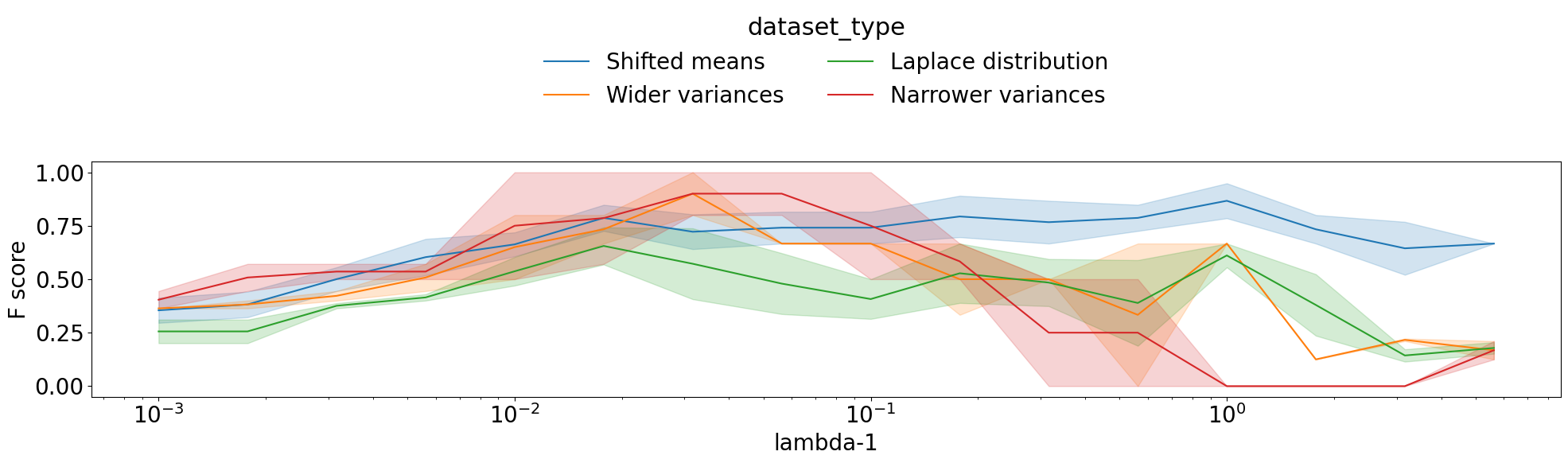
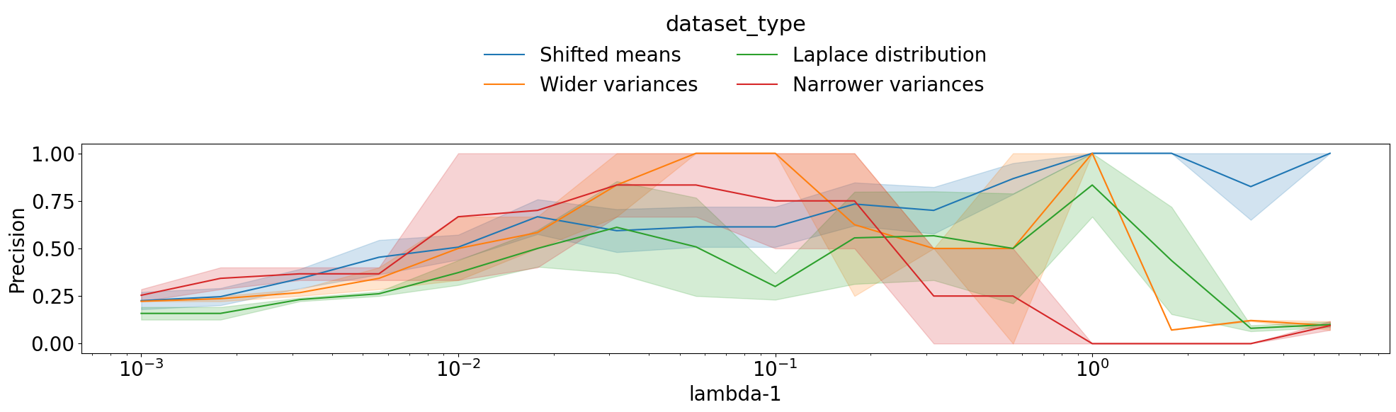
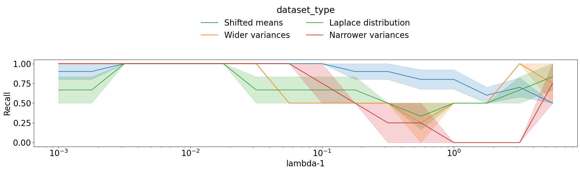
Figure 9: Effects of the regularisation parameter on the variable selection performance, discussed in Appendix E. The top, middle and bottom figures show the F score, Precision and Recall for each setting of distributions $P$ and $Q$, where the horizontal axis indicates the regularisation parameter $\lambda$ used.

Appendix F Comparing Different CV Aggregation Strategies

In the process of developing Algorithm 2 (CV-aggregation), there were several candidate ways of computing the aggregation score vector $\hat{\Pi}_{\lambda}=(\hat{\Pi}_{\lambda,1},\dots,\hat{\Pi}_{\lambda,D})^{\top}\in\mathbb{R}^{D}$ for each candidate regularisation parameter $\lambda$. Here, we compare these different choices and how we have arrived at our choice for Algorithm 2. We use the notation for Algorithm 2 in Section 4.4 in the following.

First, there are the following five ways of defining $\hat{\Pi}_{\lambda}$ based on the selected variables $S_{\lambda}^{i}\subset\{1,\dots,D\}$, where $i=1,\dots,K$:

1. “plane-variable”: $\hat{\Pi}_{\lambda,d}=\frac{1}{K}\sum_{i=1}^{K}I\{d\in\hat{S}_{\lambda}^{i}\}$ for ${d=1,\dots,D}$.

2. “p-value-variable”: ${\hat{\Pi}_{\lambda,d}=\frac{1}{K}\sum_{i=1}^{K}(1-p_{\lambda}^{i})\ I\{d\in\hat{S}_{\lambda}^{i}\}}$ for ${d=1,\dots,D}$.

3. “test-power-variable”: ${\hat{\Pi}_{\lambda,d}=\frac{1}{K}\sum_{i=1}^{K}\ell_{\rm val}(a_{\lambda}^{i})\ I\{d\in\hat{S}_{\lambda}^{i}\}}$ for ${d=1,\dots,D}$.

4. “p-value-filter-variable”: ${\hat{\Pi}_{\lambda,d}=\frac{1}{K}\sum_{i=1}^{K}I(p_{\lambda}^{i}<0.05)I\{d\in\hat{S}_{i}^{\lambda}\}}$ for ${d=1,\dots,D}$.

5. “p-value-filter-test-power-variable”: ${\hat{\Pi}_{\lambda,d}=\frac{1}{K}\sum_{i=1}^{K}I(p_{\lambda}^{i}<0.05)\ell_{\rm val}(a_{\lambda}^{i})I\{d\in\hat{S}_{i}^{\lambda}\}}$ for ${d=1,\dots,D}$.

We also have the following five ways based on the normalised ARD weights $\tilde{a}_{\lambda}^{i}$, where $i=1,\dots,K$:

1. “plane-ard”: $\hat{\Pi}_{\lambda}=\frac{1}{K}\sum_{i=1}^{K}\tilde{a}_{\lambda}^{i}$.

2. “p-value-ard”: $\hat{\Pi}_{\lambda}=\frac{1}{K}\sum_{i=1}^{K}(1-p^{i}_{\lambda})\tilde{a}_{\lambda}^{i}$.

3. “test-power-ard”: $\hat{\Pi}_{\lambda}=\frac{1}{K}\sum_{i=1}^{K}\ell_{\rm val}(a_{\lambda}^{i})\tilde{a}_{\lambda}^{i}$.

4. “p-value-filter-ard”: ${\hat{\Pi}_{\lambda}~{}:=~{}\frac{1}{K}\sum_{i=1}^{K}I(p_{\lambda}^{i}<0.05)\tilde{a}_{\lambda}^{i}}$.

5. “p-value-filter-test-power-ard”: $\hat{\Pi}_{\lambda}~{}=~{}\frac{1}{K}\sum_{i=1}^{K}I(p_{\lambda}^{i}<0.05)\ell_{\rm val}(a_{\lambda}^{i})\tilde{a}_{\lambda}^{i}$.

Note that the last approach is the one used in Algorithm 2.

Figure 10 describes the results of these candidate ways for computing the score vector $\hat{\Pi}_{\lambda}$ in Algorithm 2 and the other baseline methods. It shows F scores obtained in the same way as in Section 5.2, for two settings of the rate of the ground-truth variables $S$, $\rho=0.1$ and $\rho=0.8$.

One can observe that “p-value-filter-test-power-ard” exhibits the highest stability among the ten candidate methods for Algorithm 2. Consequently, we have decided to adopt this way for Algorithm 2.

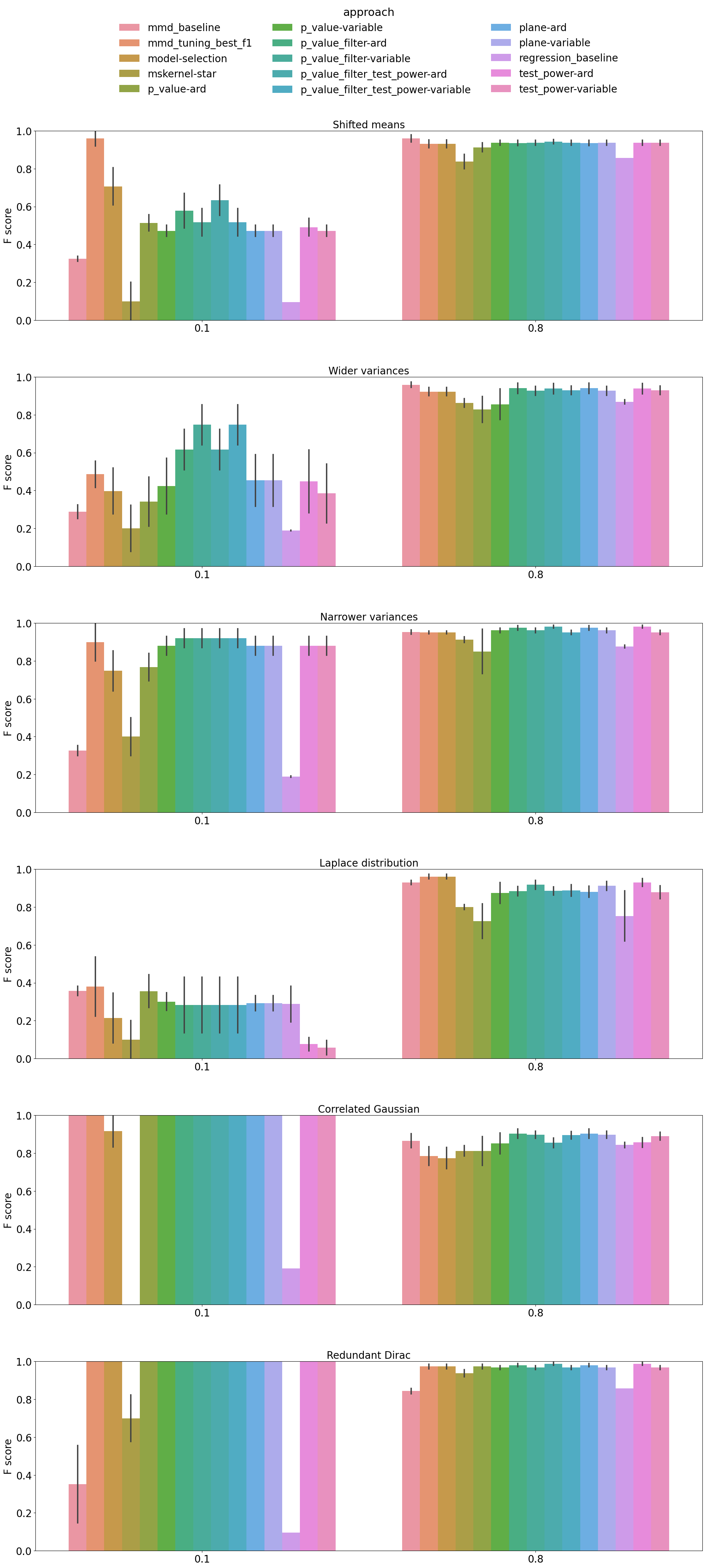
Figure 10: Comparison of the ten candidate aggregation methods for Algorithm 2 and the other baseline approaches in Appendix F. Note that "p-value-filter-test-power-ard” is the one adopted in Algorithm 2 in the main body of the paper.

Appendix G Supplementary to Section 5.2

G.1 Experiments with with Higher $\rho$

We perform the same experiments as in Section 5.2, with the rate $\rho$ of ground-truth variables $S$ being modified to $0.8$, so that $|S|=20\times 0.8=16$. Figure 11 shows the results. Compared with the results for $\rho=0.1$ in Section 5.2, all the approaches yield reasonably high scores across different settings of distributions $P$ and $Q$. The relative easiness of the setting $\rho=0.8$ can be attributed to the high number of ground-truth variables $16$. For example, if one selects all the variables, i.e., $\hat{S}=\{1,\dots,D\}$, then the Recall is $1$ and the Precision is $0.8$, so the F score is 0.89. However, in practice, one cannot take such a strategy because the value of $\rho$ is typically unknown. Given that we do not use the information of true $\rho$ for variable selection, the obtained scores can be regarded as reasonably high. Among the approaches considered, the proposed methods, model-selection and CV-aggregation, yield stably high scores across the different distribution settings.

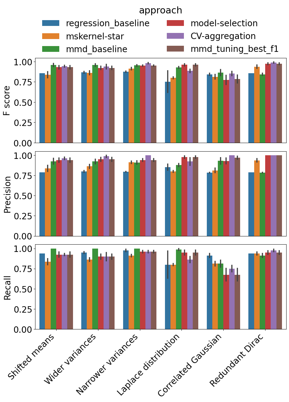
Figure 11: The results of the same experiments as Section 5.2 with $\rho=0.8$, discussed in Appendix G.

G.2 Assessing the Effects of Dimensionality

We assess the effects of the dimensionality $D$, i.e., the total number of variables, on the variable selection performance. We consider the same setting as Section 5.2, with $P$ and $Q$ being $D$-dimensional distributions in the following way.

Let $P=\mathcal{N}({\bf 0}_{D},\Sigma)$, where the covariance matrix $\Sigma\in\mathbb{R}^{D\times D}$ is diagonal with $D$ diagonal elements being

$$(\underbrace{1,1,\dots,1}_{10},\underbrace{2,2,\dots,2}_{10},\dots,\underbrace{D/10,D/10,\dots,D/10}_{10})$$

We define the other distribution $Q$ by defining how its random vector $Y\sim Q$ is generated. Let $S\subset\{1,2,\dots,D\}$ be ground-truth variables with $\rho=0.1$, so that $|S|=D\times 0.1$. Let $\tilde{X}_{S}\sim\mathcal{N}({\bf 0}_{|S|},\Sigma_{S})$, where $\Sigma_{S}\in\mathbb{R}^{|S|\times|S|}$ is the submatrix of $\Sigma$ restricted to the variables $S$. Let $Z_{S}\sim\mathcal{N}({\bf 0}_{|S|},I_{|S|})$. Then we define $Y_{S}=\tilde{X}_{S}\odot Z_{S}$, where $\odot$ denotes the element-wise product. Let $Y_{\{1,\dots,D\}\backslash S}\sim\mathcal{N}(0_{D-|S|},\Sigma_{\{1,\dots,D\}\backslash S})$. Finally, define $Y=(Y_{S},Y_{\{1,\dots,D\}\backslash S})\in\mathbb{R}^{D}$, and $Q$ is defined as the distribution of $Y$.

We consider various values for the dimensionality: $D=20,50,100,200,300,400,500$. We fix the sample size $N=200$. For each value of $D$ and each method, we experiment as in Section 5.2 and repeat it 10 times to derive evaluation scores’ means and standard deviations.

Figure 12 shows the results. As a general trend, all the approaches, except the regression baseline, experience a drop in their F scores as the dimensionality $D$ increases. This drop can be attributed to the variable selection task becoming harder for higher $D$. The decrease of the F score appears to be milder for CV-aggregation than the other methods, and the CV-aggregation attains similar F scores for the largest $D$ as mmd-tuning-best-f1, which is not implementable in practice and provides the best possible performance of model-selection.

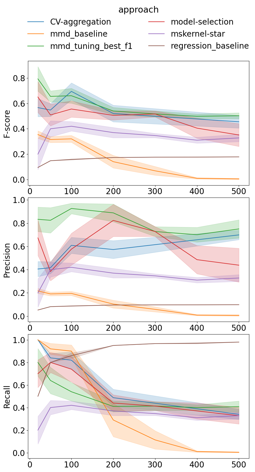
Figure 12: The results of the experiments on assessing the effects of the dimensionality $D$ in Appendix G.2. The top, middle and bottom figures show the F score, Precision and Recall for each method and each $D$, with the mean and standard deviation computed from 10 independently repeated experiments. The horizontal axis indicates the dimensionality $D$.

When comparing mmd-baseline with the proposed methods (CV-aggregation and model-selection, we observe that mmd-baseline experiences a drastic drop in the F score as the dimensionality $D$ increases, eventually resulting in the zero F score for $D=500$. In contrast, the proposed methods yield reasonable F scores even for $D=500$. This difference can be attributed to the regularisation approach used in the proposed methods, which proves to be more effective for higher dimensionality $D$.

Appendix H Supplementary to Section 5.3

H.1 Data Generation Process

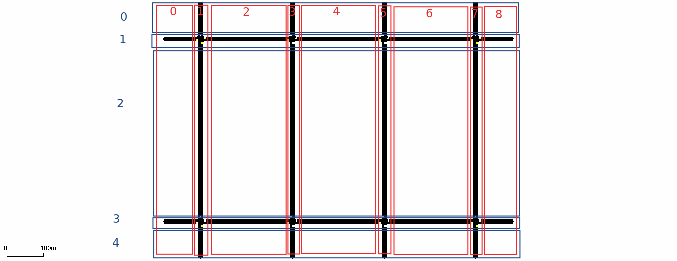
(a) The grid road network.

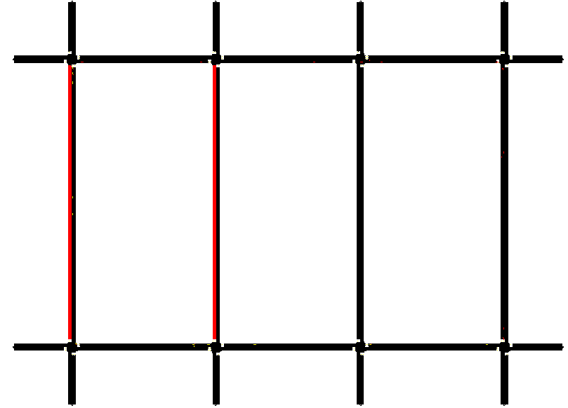
(b) The two closed lanes in the grid network, highlighted in red.

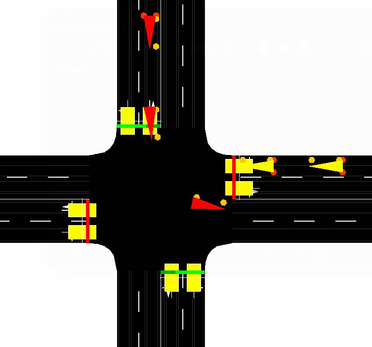
(c) An intersection in the gird network, with 8 sensors (induction loop detectors) indicated by rectangles and vehicles by triangles.

Figure 13: Illustrations of the traffic road network used in the experiments of Section 5.3, explained in Appendix H. Figure 13 describes the grid network. Each edge (= road) and each intersection are named according to the row index (blue) and the column index (red). In each scenario, there are two groups of vehicles, one travelling from the left-upper edge (row 1, column 0) to the right-bottom edge (row 3, column 8) and the other travelling in the opposite direction (from the right-bottom to the left-upper). Figure 13 highlights the two lanes blocked in scenario $Q$ in red. Figure 13 describes an intersection, where two sensors are located at the end of two lanes, resulting in eight sensors for each intersection.

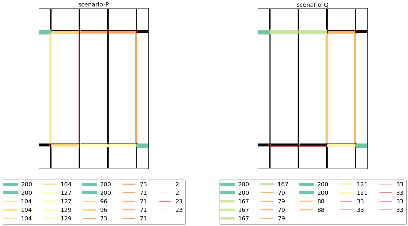
Figure 14: The number of vehicles passing each road in one simulation of scenario $P$ (left) and scenario $Q$ (right). Each edge’s line width and colour indicate the corresponding number of vehicles shown in the legend box.

We define a grid-like road network consisting of eight intersections, as described in Figure 13; we call it grid network. We define two scenarios for traffic simulation on the grid network: scenario $P$ and scenario $Q$, the latter being a perturbed version of the former. In scenario $P$, there are two groups of vehicles, one moving from the top-left corner to the bottom-right corner, and the other moving in the opposite direction. Scenario $Q$ is defined via a perturbation to scenario $P$ by blocking two specific lanes visualised in Figure 13.

Each intersection in the grid network has 8 sensors, as shown in Figure 13, resulting in 64 sensors in total in the network. Each sensor emulates an induction loops detector and measures the flow at the sensor, i.e., the number of vehicles passing in front of the sensor during one time step, representing one second in the simulation world. Each scenario consists of 3,600 time steps, corresponding to one hour, during which 200 vehicles are simulated.

We implement the grid network and the two scenarios using SUMO, a widely used traffic simulator. For each simulation, SUMO generates an XML file containing the sensors’ measurements, from which we construct a $D_{\rm sensor}\times D_{\rm time}$ matrix. Here, $D_{\rm sensor}=64$ is the number of sensors, and $D_{\rm time}=12$ is the number of time periods, each being 5 minutes. Specifically, for each $s=1,\dots,D_{\rm sensor}$ and $t=1,\dots,D_{\rm time}$, the $(s,t)$-th element of the matrix is defined as the average flow at the $s$-th sensor during the $t$-th period, calculated by taking the average of the flows of the 300 time steps (= 5 minutes) of the $t$-th period.

Since the majority of the parameters of the SUMO are controlled by the value of a random seed, an excessive seed value could produce an abnormal simulation result. To avoid such an abnormal simulation, we control the random seed by generating it as $R+\varepsilon$, where $R$ is uniformly sampled from $\{0,1,\dots,9,10\}$ and $\varepsilon$ is a Gaussian random variable with mean $1$ and variance $5$.

H.2 Results of Other Approaches

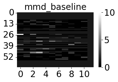
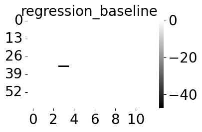
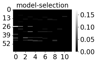
(a) Optimised ARD weights obtained without regularisation (mmd-baseline).	(b) Coefficients of the L1-peneralised linear regression (regression-baseline).
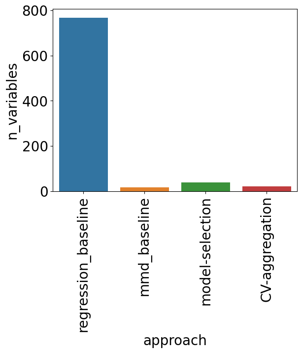
(c) Optimised ARD weights obtained with Algorithm 1 (model-selection).	(d) The number of variables selected by each method.

Figure 15: Score matrices obtained by (a) mmd-baseline, (b) regression-baseline and (c) model-selection, represented as heatmaps, along with (d) the number of variables selected by each method.

To supplement the experiments in Section 5.3, we perform the same experiments using regression-baseline, mmd-baseline and model-selection. Figure 15 visualises the score matrix obtained from each approach. The result of regression-baseline indicates an apparent failure, as it produces false positives and does not effectively identify relevant variables. mmd-baseline selects 18 variables, fewer than the 22 variables selected by CV-aggregation. On the other hand, model-selection selects 40 variables, which surpasses the other approaches.

Appendix I Variable Detection with Linear MMD Estimator

A linear unbiased MMD estimator, proposed by Gretton et al. [15], is a computationally efficient alternative to the quadratic unbiased MMD estimator (3). The quadratic estimator’s computational complexity is $O(n^{2})$ for sample size $n=m$, which can be costly for large $n$. The linear MMD estimator’s complexity is $O(n)$, thus offering a reduced computational cost, while its variance is larger than the quadratic estimator. Here, we compare the linear and quadratic estimators when used in the proposed methods for variable selection.

Given ${\bf X}=\{X_{1},\dots,X_{n}\}\subset\mathbb{R}^{D}$ and ${\bf Y}=\{Y_{1},\dots,Y_{n}\}\subset\mathbb{R}^{D}$ with sample size $n$ being odd, the linear MMD estimator is defined as

$${\rm MMD}^{2}_{l}({\bf X},{\bf Y}):=\frac{2}{n}\sum_{i=1}^{n/2}h((X_{2i-1},Y_{2i-1}),(X_{2i},Y_{2i}))$$

where $h((X,Y),(X^{\prime},Y^{\prime})):=k(X,X^{\prime})+k(Y,Y^{\prime})-k(X,Y^{\prime})-k(X^{\prime},Y)$. Assuming that $n$ is divisible by $4$, an unbiased estimator of its variance, which corresponds to (6) for the quadratic estimator, is given by [17, Eq. (7)]:

$$\check{\sigma}^{2}:=\frac{4}{n}\sum_{\ell=1}^{n/4} \left[h((X_{4\ell-3},Y_{4\ell-2}),(X_{4\ell-3},Y_{4\ell-2}))\right.$$

$$\left.-h((X_{4\ell-1},Y_{4\ell}),(X_{4\ell-1},Y_{4\ell}))\right]^{2}$$

Then, the ratio objective corresponding to (5) is defined as

$$\frac{{\rm MMD}^{2}_{l}({\bf X},{\bf Y})}{\sqrt{\check{\sigma}^{2}+C}}$$

Using this ratio objective in the regularised objective in (10), one can use the linear estimator in the proposed methods.

We perform the same experiments as Section 5.2 and make a comparison with the proposed methods using the linear estimator. Figure 16 shows the results of the F score, Precision and Recall. For all the settings of distributions $P$ and $Q$, the evaluation scores for the linear estimator are significantly lower than the quadratic estimator. The significant drop in the evaluation scores occurs even for the rate $\rho=0.8$ of ground-truth variables, which is easier than $\rho=0.1$. Specifically, in the “Wider variances” setting, the scores for the linear estimator are consistently low, approaching $0.0$. For mmd-tuning-best-f1, the linear estimator consistently performs worse than the quadratic estimator. Since mmd-tuning-best-f1 provides the highest possible F score for model-selection, the results indicate that the linear estimator is not suitable for accurate variable selection, when the sample size $n$ is not too large so that the quadratic estimator is applicable.

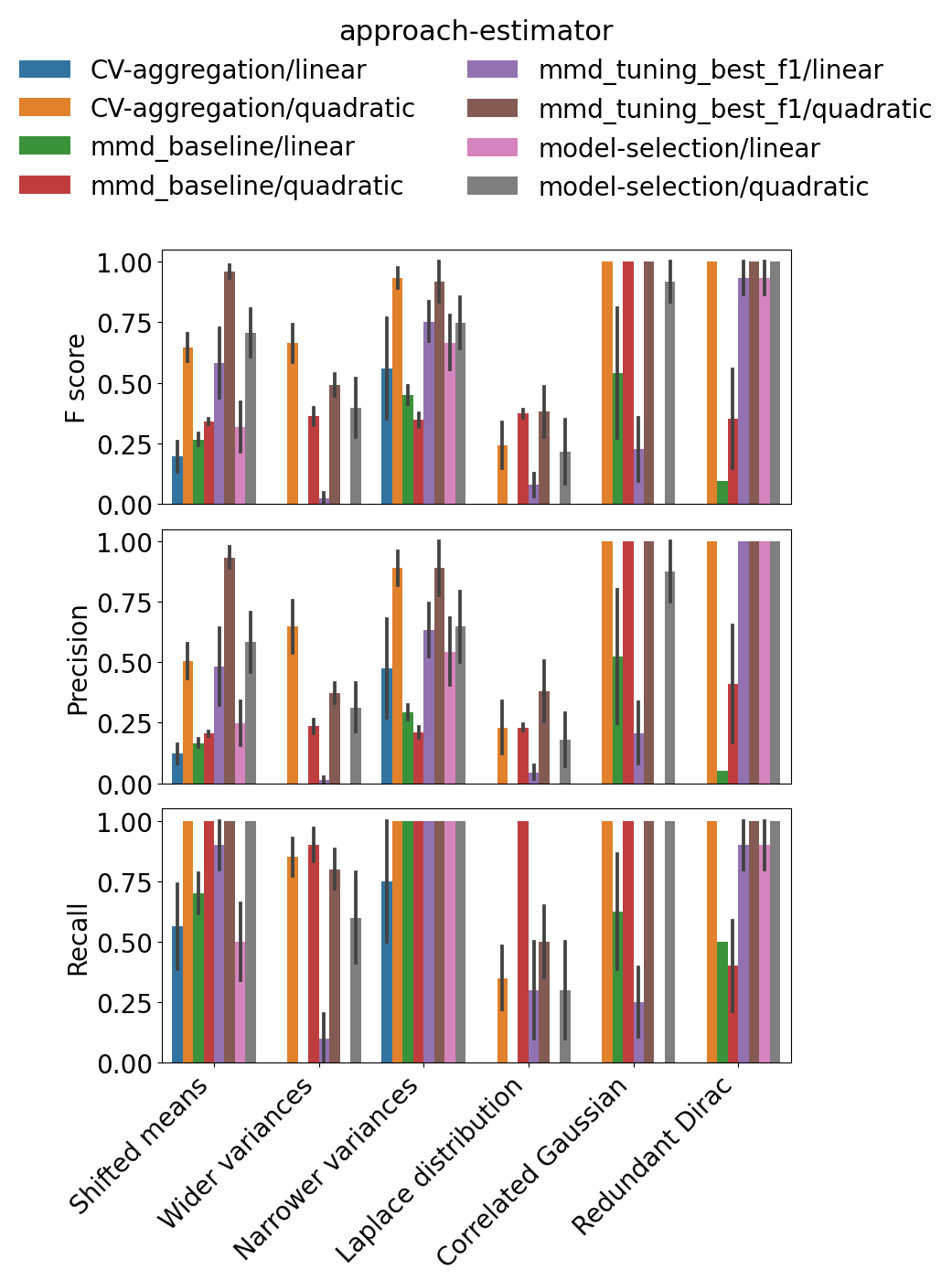
(a) $\rho=0.1$

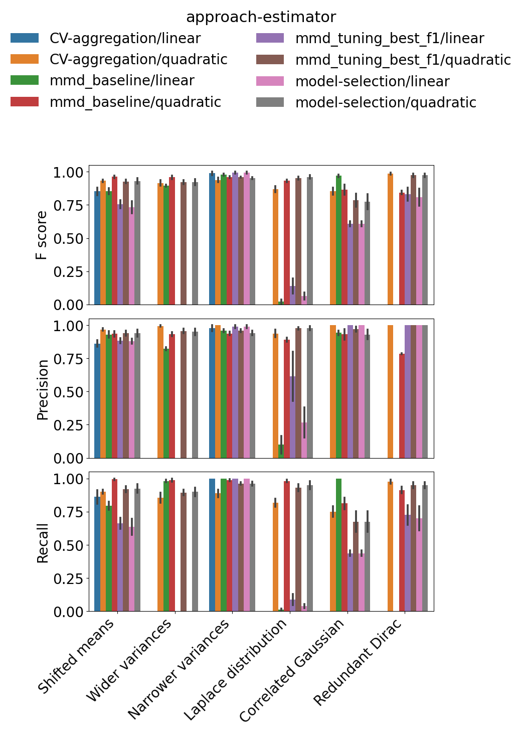
(b) $\rho=0.8$

Figure 16: Comparison of the linear and quadratic MMD estimators when used in the proposed approaches (CV-aggregation and model-selection) and other baselines (mmd-baseline and mmd-tuning-best-f1) in Appendix I. The left and right figures are the results for $\rho=0.1$ and $\rho=0.8$, respectively. The top, middle and bottom rows show the F score, Precision and Recall for each method and each setting of distributions $P$ and $Q$, with the means and standard deviations obtained from 10 independently repeated experiments. Note that the linear estimator often leads to the complete failure of variable detection, in which case no bar is shown.

Appendix J Alternative MMD-based Objective

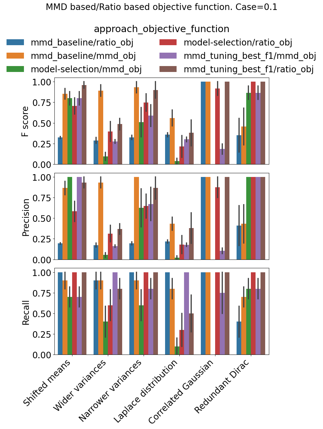
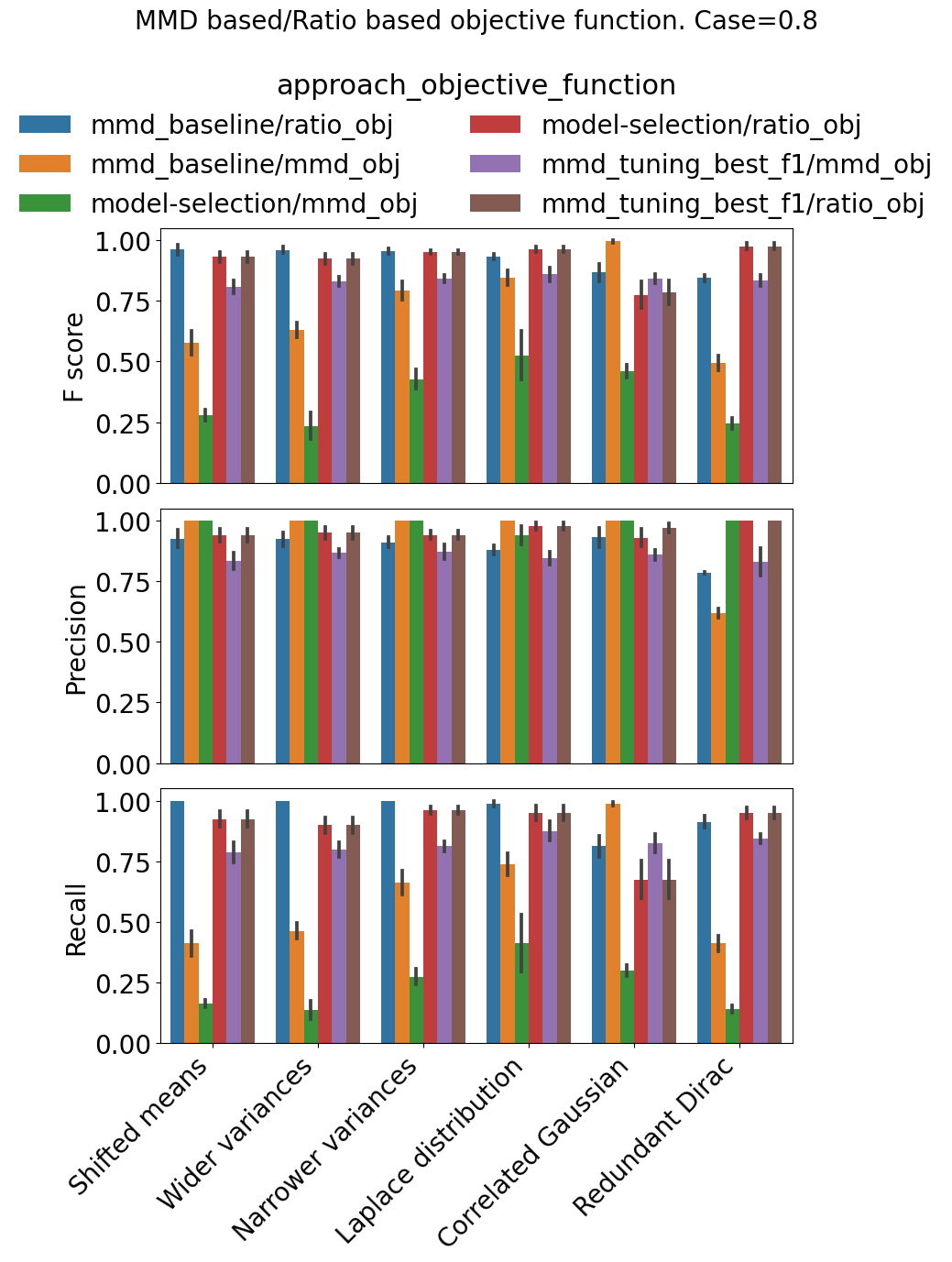
Figure 17: Results of comparative experiments between the ratio-based objective (ratio_obj) and the MMD objective-based objective (mmd_obj) in Appendix J. The left figure describes the results for $\rho=0.1$ and the right for $\rho=0.8$. Note that the evaluation scores of model_selection/mmd_obj for “Correlated Gaussian” with $\rho=0.1$ are all zero, hence no bars.

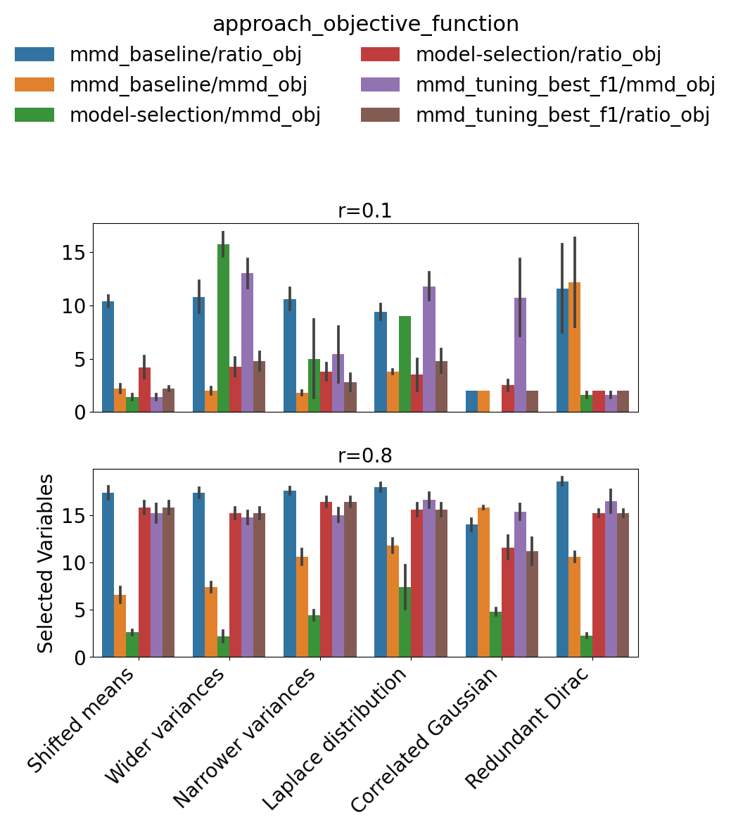
Figure 18: The number of selected variables in the comparative experiments between the ratio-based and MMD-based objective functions in Appendix J. The top figure shows the results with $\rho=0.1$, where the number of ground-truth variables is $20\times 0.1=2$. The bottom figure is for $\rho=0.8$, where the true number is $20\times 0.8=16$.

Here, we compare the proposed objective function (10) for optimising the ARD weights with an alternative objective function where the ratio objective (5) is replaced by an unbiased MMD estimate $\widehat{\rm MMD}^{2}_{U}({\bf X},{\bf Y})$ in (3), i.e.,

$$\min_{a\in\mathbb{R}^{D}}-\log\widehat{\rm MMD}^{2}_{U}({\bf X},{\bf Y})+\lambda\sum_{d=1}^{D}|a_{d}|$$ (17)

Historically, before Gretton et al. [17] proposed the ratio objective as an objective function for hyper-parameter tuning in the MMD, Sriperumbudur et al. [39] discussed that one could use the MMD itself as an objective function for hyper-parameter tuning of MMD. The latter approach optimises kernel parameters to maximise the MMD. It corresponds to removing the denominator in the ratio objective (5), thus resulting in (17). Gretton et al.  [17] showed that maximising the ratio objective yields higher test power than the MMD maximisation. We will investigate whether this property translates to the variable selection task, i.e., whether the ratio-based objective (10) leads to better variable selection performance than the MMD-based objective (17).

We perform the same experiments as in Section 5.2 for both $\rho=0.1$ and $\rho=0.8$ (recall this constant $\rho$ represents the ratio of the number of ground-truth variables over the total number of variables). Here, we compare the performance of Algorithm (1) (model-selection), mmd-baseline and mmd-tuning-best-f1, which use the ratio-based objective (10), and their MMD-based objective versions using (17).

Figure  17 describes the Precision, Recall and F scores for each setting and each method, obtained from 10 independently repeated experiments. The MMD-objective versions tend to yield lower values of the evaluation criteria than the ratio-objective versions. In particular, the former yields significantly lower Recall than the latter for $\rho=0.8$. While the MMD-based objective yields better Precision for some settings, this improvement in Precision is enabled by sacrificing the Recall. Figure 18 shows the number of selected variables for each method and each setting. It is evident that the MMD objective results in much fewer variables than the ground-truth variables for $\rho=0.8$. Based on these observations, we conclude that the ratio objective is more appropriate than the MMD objective for variable selection in two-sample testing.

References

- [1] B. Kim, R. Khanna, and O. O. Koyejo, “Examples are not enough, learn to criticize! Criticism for Interpretability,” in NeurIPS, vol. 29, 2016.
- [2] D. J. Sutherland, H.-Y. Tung, H. Strathmann, S. De, A. Ramdas, A. Smola, and A. Gretton, “Generative Models and Model Criticism via Optimized Maximum Mean Discrepancy,” ICLR, 2017.
- [3] J. Huang, A. Gretton, K. Borgwardt, B. Schölkopf, and A. Smola, “Correcting sample selection bias by unlabeled data,” NeurIPS, vol. 19, 2006.
- [4] J. Quinonero-Candela, M. Sugiyama, A. Schwaighofer, and N. D. Lawrence, Dataset shift in Machine Learning. MIT Press, 2008.
- [5] D. Lopez-Paz and M. Oquab, “Revisiting classifier two-sample tests,” in ICLR, 2017.
- [6] K. Muandet, M. Kanagawa, S. Saengkyongam, and S. Marukatat, “Counterfactual mean embeddings,” Journal of Machine Learning Research, vol. 22, no. 162, pp. 1–71, 2021.
- [7] A. M. Law, Simulation Modeling and Analysis, 5th ed. McGraw-Hill Education, 2015.
- [8] G. E. Box, “Robustness in the strategy of scientific model building,” in Robustness in Statistics, 1979, pp. 201–236.
- [9] ——, “Sampling and Bayes’ inference in scientific modelling and robustness,” Journal of the Royal Statistical Society: Series A (General), vol. 143, no. 4, pp. 383–404, 1980.
- [10] M. Yamada, D. Wu, Y.-H. H. Tsai, H. Ohta, R. Salakhutdinov, I. Takeuchi, and K. Fukumizu, “Post selection inference with incomplete maximum mean discrepancy estimator,” in ICLR, 2019.
- [11] J. N. Lim, M. Yamada, W. Jitkrittum, Y. Terada, S. Matsui, and H. Shimodaira, “More powerful selective kernel tests for feature selection,” in AISTATS, 2020, pp. 820–830.
- [12] S. Hara, T. Katsuki, H. Yanagisawa, T. Ono, R. Okamoto, and S. Takeuchi, “Consistent and efficient nonparametric different-feature selection,” in AISTATS, 2017, pp. 130–138.
- [13] J. W. Mueller and T. Jaakkola, “Principal differences analysis: Interpretable characterization of differences between distributions,” NeurIPS, vol. 28, 2015.
- [14] J. Wang, S. S. Dey, and Y. Xie, “Variable selection for kernel two-sample tests,” arXiv preprint arXiv:2302.07415, 2023.
- [15] A. Gretton, K. M. Borgwardt, M. J. Rasch, B. Schölkopf, and A. Smola, “A kernel two-sample test,” Journal of Machine Learning Research, vol. 13, no. 25, pp. 723–773, 2012.
- [16] A. Schrab, I. Kim, M. Albert, B. Laurent, B. Guedj, and A. Gretton, “MMD Aggregated Two-Sample Test,” Journal of Machine Learning Research, vol. 24, no. 194, pp. 1–81, 2023.
- [17] A. Gretton, D. Sejdinovic, H. Strathmann, S. Balakrishnan, M. Pontil, K. Fukumizu, and B. K. Sriperumbudur, “Optimal kernel choice for large-scale two-sample tests,” NeurIPS, vol. 25, 2012.
- [18] R. Tibshirani, “Regression shrinkage and selection via the Lasso,” Journal of the Royal Statistical Society (Series B), vol. 58, pp. 267–288, 1996.
- [19] N. Bonneel, J. Rabin, G. Peyre, and H. Pfister, “Sliced and Radon Wasserstein Barycenters of Measures,” Journal of Mathematical Imaging and Vision, 2014.
- [20] T. Duong and I. Koch, “Highest density difference region estimation with application to flow cytometric data,” Biometrical Journal, vol. 51, no. 3, pp. 504–521, 2009.
- [21] T. Duong, “Local significant differences from nonparametric two-sample tests,” Journal of Nonparametric Statistics, vol. 25, no. 3, pp. 635–645, 2013.
- [22] J. R. Lloyd and Z. Ghahramani, “Statistical Model Criticism using Kernel Two Sample Tests,” in NeurIPS, vol. 28, 2015.
- [23] W. Jitkrittum, Z. Szabó, K. Chwialkowski, and A. Gretton, “Interpretable distribution features with maximum testing power,” in NeurIPS, 2016, p. 181–189.
- [24] F. Cazals and A. Lhéritier, “Beyond Two-sample-tests: Localizing Data Discrepancies in High-dimensional Spaces,” in IEEE DSAA, 2015, p. 29.
- [25] I. Kim, A. B. Lee, and J. Lei, “Global and local two-sample tests via regression,” Electronic Journal of Statistics, vol. 13, no. 2, pp. 5253–5305, 2019.
- [26] J. H. Friedman, “On multivariate goodness–of–fit and two–sample testing,” Statistical Problems in Particle Physics, Astrophysics, and Cosmology, vol. 1, p. 311, 2003.
- [27] S. Hido, T. Idé, H. Kashima, H. Kubo, and H. Matsuzawa, “Unsupervised change analysis using supervised learning,” in PAKDD, 2008, pp. 148–159.
- [28] B. K. Sriperumbudur, K. Fukumizu, A. Gretton, B. Schölkopf, and G. R. Lanckriet, “On the empirical estimation of integral probability metrics,” Electronic Journal of Statistics, vol. 6, pp. 1550–1599, 2012.
- [29] F. Liu, W. Xu, J. Lu, G. Zhang, A. Gretton, and D. J. Sutherland, “Learning deep kernels for non-parametric two-sample tests,” in ICML, 2020.
- [30] W. Zheng, F.-Y. Wang, and C. Gou, “Nonparametric different-feature selection using Wasserstein distance,” in ICTAI. IEEE, 2020, pp. 982–988.
- [31] B. Schölkopf and A. J. Smola, Learning with Kernels. MIT Press, 2002.
- [32] K. Fukumizu, A. Gretton, X. Sun, and B. Schölkopf, “Kernel measures of conditional dependence,” in NeurIPS, 2008.
- [33] B. K. Sriperumbudur, A. Gretton, K. Fukumizu, B. Schölkopf, and G. R. Lanckriet, “Hilbert space embeddings and metrics on probability measures,” Journal of Machine Learning Research, vol. 11, pp. 1517–1561, 2010.
- [34] B. Efron and R. J. Tibshirani, An Introduction to the Bootstrap. CRC Press, 1994.
- [35] N. Meinshausen and P. Bühlmann, “Stability selection,” Journal of the Royal Statistical Society (Series B), vol. 72, pp. 417–473, 2010.
- [36] R. Flamary, N. Courty, A. Gramfort, M. Z. Alaya, A. Boisbunon, S. Chambon, L. Chapel, A. Corenflos, K. Fatras, N. Fournier, L. Gautheron, N. T. Gayraud, H. Janati, A. Rakotomamonjy, I. Redko, A. Rolet, A. Schutz, V. Seguy, D. J. Sutherland, R. Tavenard, A. Tong, and T. Vayer, “POT: Python Optimal Transport,” Journal of Machine Learning Research, vol. 22, no. 78, pp. 1–8, 2021. [Online]. Available: http://jmlr.org/papers/v22/20-451.html
- [37] Y. Choi, Y. Uh, J. Yoo, and J.-W. Ha, “StarGAN v2: Diverse Image Synthesis for Multiple Domains,” in CVPR, June 2020.
- [38] D. Garreau, W. Jitkrittum, and M. Kanagawa, “Large sample analysis of the median heuristic,” ArXiv e-prints, vol. 1707.07269, 2018.
- [39] B. K. Sriperumbudur, K. Fukumizu, A. Gretton, G. Lanckriet, and B. Schölkopf, “Kernel Choice and Classifiability for RKHS Embeddings of Probability Distributions,” in NeurIPS, vol. 22, 2009.