The two upper critical dimensions of the Ising and Potts models
2Sorbonne Université, Ecole Normale Supérieure, CNRS, Laboratoire de Physique (LPENS).
3Institut de Physique Théorique, CEA, CNRS, Université Paris-Saclay.)
Abstract
We derive the exact actions of the -state Potts model valid on any graph, first for the spin degrees of freedom, and second for the Fortuin-Kasteleyn clusters. In both cases the field is a traceless -component scalar field . For the Ising model (), the field theory for the spins has upper critical dimension , whereas for the clusters it has . As a consequence, the probability for three points to be in the same cluster is not given by mean-field theory theory for within . We estimate the associated universal structure constant as . This shows that some observables in the Ising model have an upper critical dimension of 4, while others have an upper critical dimension of . Combining perturbative results from the expansion with a non-perturbative treatment close to dimension allows us to locate the shape of the critical domain of the Potts model in the whole plane.
1 Introduction
The Ising and -state Potts models have a long history [1]. Let us denote by the state variable, allowed to take different values. The energy of the Potts-model on a graph with vertices and edges is defined by
| (1) |
where the first term is if and are in the same state and zero otherwise. The last term evaluates to if the spin is in state . The Ising model is the special case with . While the Potts model is originally defined for integer , it can be extended to any via the Fortuin-Kasteleyn cluster expansion [2], see section 3. A natural question to ask is whether these two expansions lead to the same field theory. While for the spin degrees of freedom, the latter was derived in the classical work by Golner [3], Zia and Wallace [4], Amit [5], and Priest and Lubensky [6, 7], a field theory for the cluster expansion is lacking. This comes with the pressing question of whether the leading non-Gaussian term is cubic as in [5, 6, 7, 8], or quartic as in [4]. This is relevant as the upper critical dimension is six for a cubic interaction, and four for a quartic one.
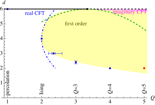
On Fig. 1 we show critical values of beyond which the critical point disappears, or equivalently beyond which this happens: Values found in the literature, are for percolation [5, 9, 6, 7], for the Ising model [10], from the numerical conformal bootstrap [11], and [12, 13]. The situation in seems debated, with values for the critical value of ranging from to : via an Ornstein-Zernicke approximation [14], via MC [13], via real-space RG [15], via NPRG [16], as well as [17] and [18], both via MC. The most precise value seems to be from Ref. [13]. In the critical value is [19, 20, 21].
The green dashed curve is our result derived in section 4.7,
| (2) |
In blue dot-dashed is shown the result in the LPA′-approximation of the NPRG [22, 23], used for Potts in [24, 16]. In this scheme, we find in agreement with [16]
| (3) |
There is an older estimation [25], obtained via the numerical solution of eleven coupled RG equations in the Wilson scheme, which reads
| (4) |
We could not reproduce this result, see section 5. Finally, Refs. [26, 25] state that for . This is incompatible with the expansion (2). On the other hand, both expansions make sense if we use Eq. (4) or (3) also in dimension : As a glance at Fig. 1 shows, the expansions in Eqs. (2) and (4) or (2) and (3) are compatible, and taken together allow for a rather precise delimination of the critical region for and . This can be obtained within various non-perturbative renormalization schemes (see section 5). For and a region (pink in Fig. 1) appears with a purely imaginary coupling. As we discuss in section 4.7, this may be an artifact of the expansion. If we start with real couplings, the yellow first-order region covers this region as well.
In the argumentation above we equated an RG flow to strong coupling with a first-order transition, as is implicitly (i.e. without proof) commonly done in the literature. We cannot exclude that the flow which apparently goes to strong coupling is towards a critical fixed point not accessible in any of our schemes. In this scenario, the boundary of the critical regime remains unchanged, but the interior of the “first-order” region may become second-order, or split in a first-order and a second-order regime.
To complement our introduction, let us mention field-theory results for the cubic [8, 27, 28, 29], quartic [27] and quintic theories [30], which each are consistent below their respective upper critical dimensions, and which we expect to be (higher critical) conformal field theories (CFT). Expansions as in Eqs. (4) or (3) also appear in [31].
In this work, we first derive the exact field-theoretical action in the spin formulation (section 2), followed by the exact action of the cluster expansion (section 3). By exact we mean that on an arbitrary graph the field theory produces the partition function and all correlation functions, without any approximation.
When evaluating these exact actions for regular lattices, e.g. the cubic lattice in dimensions, and taking a continuum limit, the action expanded in the fields contains an infinity of interactions. In order to set up an efficient RG scheme, we follow the standard procedure to retain solely the most relevant terms. The result of this procedure is different in the spin and cluster expansions: In the cluster expansion, the leading interaction is cubic for all , leading to . In the spin formulation, the Ising model is special, since its symmetry under a reversal of the field (the magnetization) excludes a cubic vertex, leading to an upper critical dimension . This suggests that for the Ising model spin-correlation functions are given by mean-field theory in dimensions between four and six. However, the probability that three sites are in the same cluster is given by the non-trivial cubic theory. The latter predicts to leading order in that
| (5) |
where is the probability that , , and are in the same cluster, and likewise for the terms in the denominator. While the functional form of is imposed by global conformal invariance [32] as written, the amplitude is non-trivial, and measurable in a numerical simulation. We report below in Eq. (89) a similar result for other values of .
The article is organized as follows: In section 2, we derive the field theory for the spin expansion, followed by the field theory for the cluster expansion in section 3. Section 4 treats the ensuing field theories perturbatively, and calculates the structure constant. In section 5 we treat the -state Potts model via the non-perturbative renormalization group, which allows us to draw the phase diagram in the whole plane. In section 6 we conclude. Some technical details on the Potts algebra are relegated to appendix A.
2 Spin expansion
We start with a reminder or the spin expansion for the Potts model. Consider the -state Potts model. Following [3, 4], we represent each state as a vector111While this representation is heuristically appealing, and allows one to coarse-grain spin degrees of freedom, it may be but one of various distinct possibilities. We will see a systematic procedure for the cluster expansion in section 3.
of length , and a scalar-product of between distinct vectors,
| (6) | |||||
| (7) | |||||
| (8) |
The normalizations are chosen for convenience. As an example, for we have , while for the three vectors lie in the plane with an angle of between them. We refer to appendix A for details on this construction.
The energy of the Potts-model in this spin representation, in the presence of a magnetic field is
| (9) |
According to Eq. (7),
| (10) |
With the help of this identity, Eq. (9) can be rewritten as
| (11) | |||||
To obtain the effective action, we follow the standard procedure [33]: introduce an auxiliary field to decouple the interaction, sum over the spins, and finally perform a Legendre transform w.r.t. the auxiliary field. We start with
| (12) |
As , the matrix element can be chosen to our liking, allowing us to ensure that the inverse kerne exists. The double sum over runs over all vertices, and , but if . To reduce clutter, we drop the notation that for the remainder of this section.
We now decouple the interaction,
| (13) | |||||
Note that in order for the path integral to converge, is chosen imaginary. Summing over spins yields (for each site , dropping the index)
| (14) | |||||
| (15) |
where we defined
| (16) |
By construction . This allows us to write
| (17) | |||||
From the first to the second line we shifted , and finally replaced by . The change in measure is reflected by a new normalization constant . The last line is
| (18) |
with the action (signs: )
| (19) |
We note that and . We can therefore write
| (20) |
We now construct , the Legendre transform of . The result, keeping only the most relevant terms, is
| (21) | |||||
3 Fortuin-Kasteleyn cluster expansion
3.1 Basics of the cluster expansion
The Fortuin-Kasteleyn (FK) cluster expansion for the Hamiltonian (9) is [2]
| (22) | |||||
where runs over all possibilities to use the term , i.e. over all subsets of edges . Each cluster is the disjoint union of connected components ,
| (23) |
We now interchange the two sums [2],
| (24) | |||||
The state is constant on each connected component , and is independent on two different components. If , then
| (25) |
If independent of , then
| (26) | |||||
Thus for and small
| (27) |
where
| (28) | |||||
| (29) | |||||
| (30) |
3.2 Sampling cluster configurations from spin configurations
According to the arguments given above, cluster configurations can be sampled from spin configurations:
-
(i)
sample a spin configuration with the weight ,
-
(ii)
identify regions of equal spin as a spin domain. We consider a bond between two equal spins to belong to this spin domain.
-
(ii)
for each such bond inside a spin domain, remove it with probability .
-
(iv)
each spin domain is by this construction decomposed into one, or several, clusters (i.e. connected components) of the FK expansion.
An important result of this construction is that the clusters of the FK expansion live inside the spin domains.
3.3 An exact lattice action for the cluster expansion
Let us start from Eq. (22),
| (31) |
which we rewrite as
| (32) |
Here
| (33) |
We claim that Eq. (31) is produced by the path integral over all and , with action (weight)
| (34) |
Proof: The first term in the action is a term for each site . This term is introduced to have a Gaussian measure on each site, with expectation values
| (35) |
The last term gives a factor of per edge. The square root in Eq. (34) corrects for the fact that the product contains both the terms and . Expanding at in powers of generates all possible terms in the cluster expansion, and each bond in the cluster expansion appears with a factor of . (Note that the coupling on bond may differ from bond to bond, and our derivation remains valid for random-bond models).
The next thing to achieve is to contract the fields, for a given term in the cluster expansion. Due to the rules (35), the only available contractions are with the term . Writing down for each factor of , we need to evaluate
| (36) |
Thus whenever the cluster-expansion contains the term , our action forces the and fields to have the same index . This gives a factor of per cluster . This completes the proof. For the most interesting case of vanishing magnetic field, , this reduces to .
3.4 Expansion of the cluster action in the fields
We can expand Eq. (34) in powers of the field. This will be relevant to access the critical theory in dimensions. With this in mind, we expand the action up to third order, putting . We start with the auxiliary formula
| (37) |
This implies that the corresponding contribution to the action from Eq. (34) reads
| (38) |
The next contribution to from Eq. (34) reads
| (39) |
where we used that and this contribution is summed over . Therefore, up to a constant,
3.5 Integrating out
Since only appears quadratically in the action (3.4), we can integrate it out. (Higher-order terms have to be dealt with when including terms of order .) To do so, we take the saddle point
| (40) |
where again we used . This can be rewritten as
| (41) |
where
| (42) |
is the lattice Laplacian. There is a mass term ,
| (43) |
where coord is the coordination number, i.e. the number of nearest neighbors. (The signs are for , i.e. ferromagnetic couplings.) Then Eq. (41) can be inverted,
| (44) |
This gives
| (45) | |||||
Note that the contribution from the determinant in the integration over is independent of , thus a constant which can be neglected.
3.6 Decomposition into scalar and traceless parts
The next step is to decompose into irreducible representations of the symmetric group (which exchanges the flavours of the Potts spin), see e.g. [34, 35, 31],
| (46) |
is the vector representation with Young tableau and dimension , while is the scalar representation with Young tableau and dimension 1. Both are irreducible for . This gives for the action
| (47) | |||||
Note that the terms non-linear in which come from have all canceled. This property is exact and holds to all orders. It can be traced back to
| (48) |
Thus there are no non-linear terms in from the vertex! The only terms of order larger than two that may appear are from the quartic term (or higher).
Let us write the action with these simplifications. The mode is massive with squared mass (second line of Eq. (47)), and expectation
| (49) |
However decouples inEq. (47). The remaining action for reads
| (50) |
This is a cubic field theory, for any value of .
The modes have a bare mass
| (51) |
3.7 Local observables
A key information to know is which cluster site belongs to. This can be achieved by dropping the sum at site . Formally, the operator which tells whether site is in a cluster of color is
| (52) |
The denominator takes out the corresponding term from the action (34), and replaces it by the same term without the sum. As constructed,
| (53) |
To access the probability that different sites are in the same cluster, we define its connected part,
| (54) |
Expressed in terms of and , this reads
| (55) |
The probability that sites are in the same cluster is proportional to
| (56) |
4 Renormalization: expansion
The renormalization group for the -state Potts model is usually performed in momentum space. Here we present this standard calculation in position space. The advantage is that the 3-point function encoding the structure function is then easily evaluated.
4.1 Relevant relations and normalizations
Using the definition of the -function, one first shows that
| (57) |
This allows us to Fourier transform power laws according to
| (58) |
Eq. (58) for implies
| (59) |
In order to reduce as much as possible geometric factors, we introduced the -dimensional volume element
| (60) |
A useful relation is
| (61) |
This is proven by going to momentum space w.r.t. to and , multiplying the two momentum dependent functions, and transforming back.
Following CFT conventions, field theory is constructed with propagators normalized such that
| (62) |
The bare Lagrangian in these normalizations is
| (63) |
The index is the field index, while the index refers to bare quantities.
4.2 Renormalization scheme
Following the standard field-theoretic scheme [4, 36, 37, 5], renormalization is performed by introducing RG-factors,
| (64) |
Here all quantities are renormalized, contrary to Eq. (63), where they are bare. The relation between bare and renormalized quantities is
| (65) | |||||
| (66) |
This yields the function , full field dimension , and anomalous exponent as
| (67) | |||||
| (68) | |||||
| (69) |
4.3 Vertex renormalization
There are two types of correction at 1-loop-order. The first is a correction to , the vertex. Graphically, it can be written as
| (70) | |||||
A thick solid line signifies the term in the propagator, whereas the dashed line does not force the indices to be equal; the accompanging factor of is written explicitly. The diagrams in the second line vanish due to , and are not reported in the final result. Including all combinatorial factors, the perturbative result for the cubic vertex is
| (71) |
The combinatorial factors are: from the third-order expansion of the exponential function; a factor of for each additional vertex as written in the action (64); a factor of per vertex for choosing the uncontracted leg; a factor of for contracting a first chosen leg; a factor of for the remaining contraction. The diagram having 3 propagators, one can for each of them choose the contribution proportional to the -function for the indices, or in any of the three use the term without a -function, for a total of ; using for two or three propagators the term without the -function would break the connectedness of the diagram. The final factor is the integral. Regularized at scale it is
| (72) | |||||
We used Eq. (61). Note that we could equivalently put a cutoff on both and , see [38, 39, 40]. The remaining integral gives
| (73) |
Therefore with , and the remaining ’s evaluating to 1,
| (74) |
This identifies
| (75) |
4.4 Renormalization of the elastic term
The second contribution is the renormalization of , the elastic term (wave-function renormalization). Similarly to what has been done in Eq. (70), the group-theoretical factor is
| (76) |
Due to , the last term does not contribute. Therefore, this relation can be simplified to
| (77) |
Writing explicitly the fields to keep track of the derivatives, the contribution to reads
| (78) | |||||
The first is due to the fact that we have , the is from the second order in , then combinatorial factors, group factors, and the integral. In the third line we used rotational invariance to discard the first-order term in , and simplify the second term. Regrouping and dropping the UV-relevant term gives
| (79) | |||||
The last term is the free Lagrangian density, yielding the field renormalization factor (for )
| (80) |
4.5 RG functions
The -function as defined in Eq. (67) is
| (81) |
The fixed point is at
| (82) |
Note that for the fixed point is real, while for larger it is imaginary. The latter situation contains the Lee-Yang class, to which our RG equations reduce in the limit of . Intuitively this can be understood by remarking that for the constraint becomes negligible, and the Lagrangian (63) reduces to that of decoupled Lee-Yang field theories.
4.6 3-point function and structure factor
We now consider the 3-point function which forces all external indices to be in the same cluster,
| (85) | |||||
where we used the star-triangle identity. The latter reads
| (86) |
| (87) |
It holds whenever . Since the integral is convergent in , we can evaluate it there, ensuring that the latter relation is valid. This gives the leading term in ,
| (88) |
Using Eq. (82) yields
| (89) |
We give the three most interesting values
| (90) | |||||
| (91) | |||||
| (92) |
Note that for the Lee-Yang class, the definition involves an imaginary coupling, so this agrees with [41]. In dimension this question has been solved analytically by relating [42] the structure constant to the so-called DOZZ formula of imaginary Liouville conformal field theory [43], a result which has been checked numerically [44] and also generalised to a larger class of operators [45]. The structure constant is expressed in terms of the Barnes double gamma function, whose evaluations for integer read [44]
| (93) |
Our result is astonishingly precise for percolation in . We will see that already for the Ising model this expansion can no longer be used below dimension , see section 5.4. Finally, it is curious that all known values of lie close to , a value natural in dimensions and , see appendix B.
4.7 The upper boundary of the non-critical domain
The -function up to 2-loop order [8, 46], divided by the coupling to exclude the Gaussian fixed point, reads after some rewriting
| (94) |
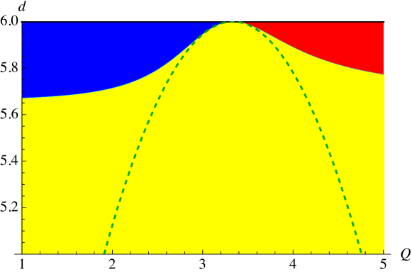
The necessary condition for having a non-Gaussian fixed point is . As any quadratic equation, it has two solutions, of the schematic form . The solution relevant for us is the one which vanishes for . As Fig. 2 shows, as a function of and , there is a domain with one real positive solution (in blue), a domain with one negative real solution (in red), and a domain where no real solution exists, but a pair of complex conjugate ones (in yellow). The boundary is given by the line where vanishes. To leading order in , this reads
| (95) |
This is the green dashed line in Fig. 2.
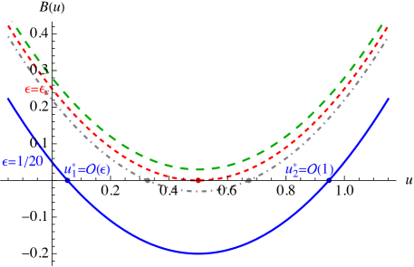
To go beyond leading order, we need a more systematic procedure. Consider Fig. 3, where for visualization we plotted . The coefficients have the same signs as in Eq. (94), and the qualitative analysis for Eq. (94) is the same. One sees that for small, there is a perturbative solution , and a non-perturbative solution with . The minimum of is between these two solutions, and is negative there. Up to ( in the plot), there is still a solution for which both . For larger values of , no real solution exists, but a pair of complex conjugate solutions.
Our strategy to continue is clear: We demand that
| (96) |
It is convenient to first write the latter equation,
| (97) |
Note that this equation is independent of , i.e. dimension. It is solved by making for an ansatz as a power series in . Asking that than gives as a function of . Using the 5-loop series of [46], partially given in [29, 28] and to 3 loops in [8], we get
| (98) | |||||
This series seems to be Borel-summable for . We were unable to improve the plot on Fig. 2, because even if Borel-summable, the radius of convergence seems to be very small222We tried directly taking 3-loop to 5-loop predictions, Padé-Borel resum them, and to write the (two branches of the) inverse series for as a function of ..
For , all terms of the series are negative, which indicates that a branch cut singularity starts there. We come back to this questions in our NPRG treatment, see section 5.3.2.
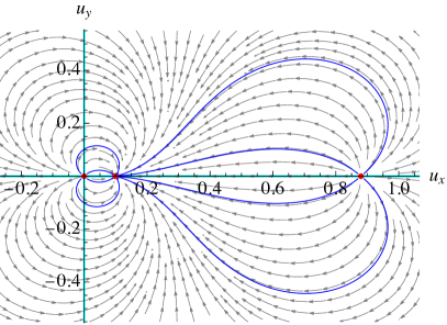
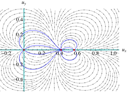
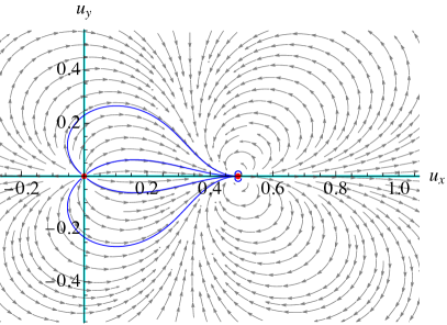
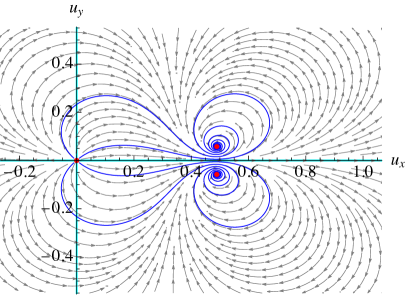
It is interesting to see what happens to the RG flow in the complex plane. This is done on Fig. 4. For small (here , top left plot) the critical fixed point lies close to the Gaussian one, while a tricritical (bi-unstable) fixed point is at . Increasing (top right), the critical and tricritical fixed points approach, until they merge at (lower left plot). Up to this value of , all fixed points lie on the real axes . Increasing further, a pair of complex-conjugate fixed points emerges. Since the critical fixed point for smaller is globally attractive and the flow at large couplings is not rearranged, the pair of complex-conjugate fixed points is also globally attractive, with the RG flow spiraling in (complex eigenvalues).
5 Non-perturbative renormalization
5.1 Flow equations
Mapping out the full phase diagram is impossible by relying solely on controlled expansions. Here we study the full phase diagram using the different non-perturbative RG schemes, LPA, LPA′, LPA∗ and Wilson’s original approach. For the Potts model, this line of research was pioneered in [25] (Wilson scheme), and continued in [24, 16] (LPA′). The idea is to start from the action
| (99) |
where333In most of the current literature [24, 16] the expansion is written in terms of the unconstrained basis, see appendix A. This is much more tedious to implement than in the constrained basis used here.
| (100) | |||||
The correction to the effective action in the Wilson scheme is obtained by integrating out the largest wave-vector mode, here with . (The index structure is given later.)
| (101) | |||||
This leads to
| (102) |
In contrast, in NPRG one has
| (103) | |||||
This gives
| (104) |
Note the power of in the denominator, which is larger by one than in Wilson. The difference in combinatorial factor can be rationalized as follows: The Wilson cutoff is a hard cutoff, which allows one to integrate out the fastest mode, leading to . The cutoff used for the LPA is a soft cutoff, the calculatorially easiest choice is the Litim cutoff [47]
| (105) |
With this choice the IR flow reads
| (106) | |||||
Scaling and absorbing the volume factor gives Eq. (103).
Finally, we need to rescale and , and add indices. This leads to the NPRG equation (IR flow)
| (107) |
The first remark is that a global prefactor (the normalization of space) can be absorbed by a rescaling of , as this changes the rescaling terms which are linear in , but not .
We have written explicitly the index structure of each term in the Potts model, with the matrix and the projector (with the same index structure as the propagator) defined as (see appendix A)
| (108) |
The factor of depends on the cutoff and , and reads
| (109) |
We added an anomalous dimension for the field, or exponent . The latter is obtained from
| (110) |
The global prefactor is fixed s.t. for the -function vanishes at ,
| (111) |
This is equivalent444For the Wilson scheme and this reduces to Eq. (83) noting that , and that there is an additional explicit factor of in Eq. (102) as compared to the field theory. to Eq. (83) for . When improving LPA, we call this scheme LPA∗, when improving Wilson we call it Wilson∗. It is slightly different from what is used in the NPRG literature [16], and termed LPA′: There is an additional factor of multiplying the r.h.s. of Eq. (106). The reader may wonder about the denominator in Eq. (110). A heuristic way to derive this is to take one derivative w.r.t. the passing momentum , which is similar to a variation of the squared mass , increasing the number of factors in the denominator by 1.
All these subtleties are unimportant close to the upper critical dimension 6, and for lower dimensions everything we do here seems badly controlled: This is seen when comparing the different approximation schemes in order to see how robust the results are. This is done later; we will see that LPA′ and LPA∗ (at the same field order) are almost indistinguishable, but that for small the results strongly depend on the maximal number of fields allowed.
5.2 Implementation
We implement the above program by going up to order 6 in the fields, as suggested by Eq. (100). We then calculate the corrections to up to order . This perturbative treatment, also used in [24, 16] properly accounts for the algebraic structure of the Potts propagator555This is possible at fixed , when restricting to the spin degrees of freedom. As an example, for , there are two independent fields, and the theory can be written in terms of and . For non-integer this is not possible.. We do not know of a truly non-perturbative approach at non-integer , where as a function appears in the denominator.
We then start somewhere below dimension , propose an initial condition with , and try to evolve to a fixed point of the -function (107). We have several routines to do so: The first tries to integrate the flow-equation itself, in which we have reversed the flow for , which is a relevant coupling: it has an RG eigenvalue close to 2. The other algorithms we implemented are different routines to find a nearby minimum of (steepest descent, Newton iteration, Monte Carlo). Once we find a solution, we can walk in the plane, following this solution under a change of or , until we reach the critical line. What happens there depends on where we start. Let us discuss the different sectors. If not stated differently, we use the LPA∗ scheme where is truncated at order , and which we denote LPA. Results for LPA are almost indistinguishable.
5.3 Branches
5.3.1 Upper left sector ()
For fixed and , or (close to ) we propose a solution with , and the remaining . Using the -function where the flow of is reversed, these couplings converge to a critical point of the -function. Linearizing the -function around this solution we find one relevant EV, while all remaining EVs are irrelevant. We then decrease , and follow the fixed point in question by again minimizing the -function. At some point, the second-largest EV becomes zero, at which point it merges with a tricritical fixed point. Further decreasing we loose this fixed point and as a consequence run to strong coupling; in practice, our algorithm no longer succeeds to finds a solution, and blows up. We identify this dimension as . If we worked hard, we should be able to find a tricritical point, which merges with the former fixed point at . One observes that close to this eigenvalue behaves as a constant times . Close to , the curvature of this curve is close to what is expected within the NPRG. We had expected to see the expansion of Ref. [25] given in Eq. (4) to agree with our Wilson approximation, but this is not the case. As we do not have the equations of [25] to compare with, we cannot make this comparison quantitative.
Finally, we could try to follow the fixed points into the complex plane. We did not pursue this approach here since we would have to double the number of couplings passed to our routines.
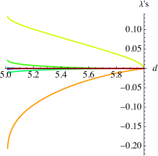
5.3.2 Upper right sector ()
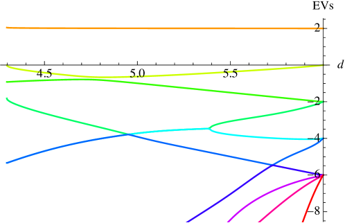
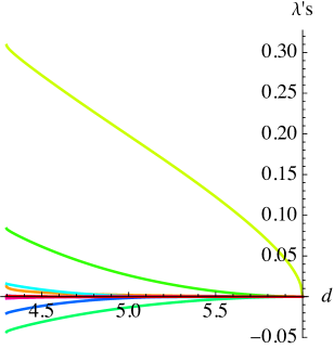
The scenario observed for is also observed for , after multiplying the odd couplings by a factor of . However, close to , we see a different behavior, for which an example at is shown in Fig. 7. What we observe is that at a dimension the third-largest EV merges with the second largest one, and together they wander off in the complex plane. Decreasing further to , they both become relevant, albeit with a non-vanishing imaginary part. Below the latter dimension, the RG equation runs to strong coupling, so . We suspect, however, that the critical dimension is already reached at ; otherwise the critical dimension as a function of seemingly jumps at , which we have a hard time believing. On the other hand, up to 5-loop order the perturbative series for has only positive terms for , whereas the series alternates for . This may signal a non-analytic behavior for for . Our results indeed show a roughly linear dependence of , on .
It is equally possible that the approximations used, either in the NPRG or its implementation, are inadequate. There should not be a problem with the numerical evaluation of the zeros of the -function, which is done with 400 digits of precision (more than 10 times machine precision).
We finally note that within the NPRG in the limit of the copies not necessarily decouple, as it is possible to have a fixed point with an inter-copy coupling (as ) persist when taking , even though when starting with decoupled models at , these inter-copy interactions are not generated. As a result, this limit may be as subtle as the large- limit for Random-Field [48, 49].


5.3.3 Lower branches
The lower left branch is more difficult to reach, as generically most initial conditions either blow up when evolving them with the “improved” -function, or converge to multiply unstable (tricritical or higher) fixed points. We also tried to walk down for , which is possible, but then we failed to cross the line , where some of the operators decouple. Our successful strategy was to generate random couplings , , and , with for the rest. We then used steepest descent for and towards a fixed point, and stop when this fixed point has one relevant direction. The successful trial for LPA converged to
| (112) |
To proceed, we start at this point, and then walk in the plane until we hit the boundary of the critical region. The result is shown in Fig. 5. It is reassuring to see that the various LPA approximations all have the same parabolic shape around , . Depending on which approximation is used, the critical line follows this parabola further, or less. The results of Ref. [16] (green points with error bars closes to ), which go up to order 9 in the field, are able to follow this parabola a little further than we do, without noticeably deviating from it. When comparing the different schemes, one observes that all schemes follow the critical parabola given in Eq. (3) for , and that including more fields allows one to follow this parabola further. Including also increases the range for which this is possible, i.e. before grows again. There is only a minimal difference between LPA′ and LPA∗. We were unable to find a value of the couplings to repeat this analysis in the Wilson scheme. We conjecture that this parabola is close to the critical curve, and a slight deformation to pass through , is a good approximation for the true critical curve. This is the rational behind Fig. 1.
Going back to Fig. 5, we observe that the critical curve becomes horizontal for large , and by walking down we find a second curve as indicated in Fig. 5. While this may well be an artifact of the scheme, it leaves open the intriguing possibility that in dimension the Potts model has a window of values for for which it becomes critical again.
5.4 Ising ()
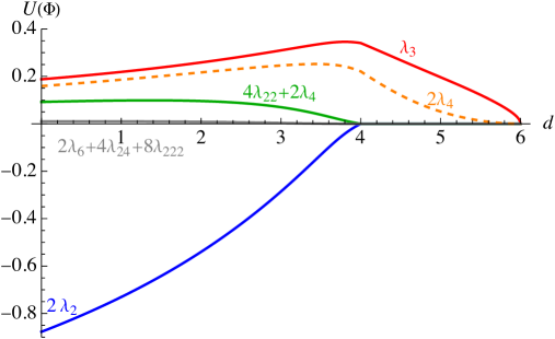
We succeeded to walk down at from to . The result is shown on the left of Fig. 8, using LPA: since , the schemes are identical, i.e. . We can then project onto the Ising spin variables, by writing down in terms of and , then setting , . This gives the potential visible in the spin sector of the Ising model.
| (113) |
As can be seen in Fig. 8, these couplings vanish in dimensions , even though itself is non-vanishing there. This is the Gaussian fixed point for the spin-degrees of freedom in dimension . Below dimension , the quartic coupling visible in the spin theory, see Eq. (113), becomes non-vanishing. Descending below also the sextic couplings become visible, albeit small.
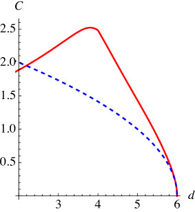
This plot leads to the conjecture that the structure constant , at leading order proportional to , grows from dimension to dimension , before descending again. Assuming that the structure constant is indeed proportional to , and normalizing s.t. the -expansion is matched, gives the plot on the right of Fig. 8. It shows clearly that the expansion for the structure constant given in section 4.6 will break down in dimension .
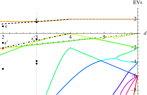
There are some interesting tests we can perform, see Fig. 9: The largest eigenvalue in the stability matrix of the -function is , which equals 2 in dimensions , and has -expansion below dimension . This is well respected in the NPRG, see the topmost curve on Fig. 9. The exponent is the second-largest eigenvalue. For the cubic coupling it has 1-loop dimension in (gray dotted in Fig. 9) which is valid for , while (gray dot-dashed in Fig. 9) seems to be a decent approximation down to . The quartic coupling has 1-loop eigenvalue . The NPRG flow respects these expansions. The operator content seems rather sparse in dimension , and misses higher scalar operators known in the bootstrap [50]. This should improve upon increasing the maximum field dimension in the NPRG.
5.5
We can also walk down from for . For , this is possible down to dimension . For the system of RG equations seem to become degenerate in dimension , see Fig. 10. For this happens already in dimension . This may be a sign for a first-order transition (which is unlikely given what we know about percolation), or a technical problem. In the latter case it may indicate that the -expansion is valid only down to dimension . Another degeneracy is observed when trying to walk in dimension from to . It would be interesting to analyze this further.
6 Discussion and conclusion
We showed that there are two distinct field theories for the -state Potts model, one for the spin degrees of freedom, and one for the cluster degrees of freedom. The latter is exact on any graph, and does not impose the representation of the states as a vector in . As a consequence of these different representations, the Ising model has two distinct upper critical dimensions, for spin observables, and for cluster properties. This allowed us to derive an explicit prediction for the 3-point function, equivalent to the structure constant of the underlying CFT. We hope that numerical simulations will soon verify this prediction.
An interesting question is how this extends to other values of . Our analysis shows that for the Potts model has a second-order transition only outside a non-critical region. Its boundary is perturbatively controlled close to , with a parabola, open to the bottom in the plane, emanating from , , see Fig. 1. Another bounding parabola open to the right, emanates from , , with a coefficient which can be estimated within a non-perturbative approach. As discussed in the introduction, there is ample numerical and analytical evidence that the lower bound of the non-critical region exits as well, even though it is yet badly approximated by any RG scheme. We are working on a expansion to remedy this. One should also be able to expand around the point and , similar to what was done in [52] (up to an unknown coefficient) for the model (around ), see also [53]. Going back to and , we note that a new critical theory emerges when rotating all odd couplings into the complex plane. Taking this connects to the well-known Young-Lee universality class.
Since the clusters of the FK expansion live inside the spin clusters (see section 3.2), spin correlations cannot fall off faster than cluster correlations. Written for the field-dimension , or the exponent , this reads
| (114) |
Eq. (84) shows that to 1-loop order, and for
| (115) |
This property persists to higher orders, and especially for close to (). For the Ising model for , and the bound is saturated.
Perturbative RG near dimension 6 gives a very clear picture of what happens when we enter the “first-order” domain: allowing the couplings to become complex, the critical and an additional tricritical point merge, and then wander into the complex plane, forming a pair of complex conjugate critical fixed points. In contrast, when starting with real couplings, the RG flow runs to strong coupling, a sign (but no proof) that the phase transition in this domain is first order. We conjecture that this pair of complex fixed points can be observed in the -states Potts model, either via numerical simulations in , or via transfer matrix in . A CFT with couplings at a complex fixed point was indeed proposed in for , with explicit predictions for [54, 55].
Acknowledgements
We thank Mikhail Kompaniets and Andrey Pikelner for providing us with the 5-loop perturbative expansion for the -state Potts model, and John Cardy, Bernard Julia, Mehran Kardar, Adam Nahum and Slava Rychkov for stimulating discussions. We are most indebted to Andrei Fedorenko for generously sharing his expertise on the NPRG, and for questioning all our assumptions.
Appendix A Algebraic objects
The construction for a basis of the -state Potts model works as follows: Chose vectors , with
| (116) |
s.t.
| (117) |
We use a dot for scalar products in -space (roman indices, dimension , unconstrained basis); a circ “” denotes the scalar product in -space (greek indices, dimension , constrained basis). These vectors can be constructed recursively, see [3, 4], Eq. (2). They satisfy
| (118) |
Proof:
The inverse relation is
| (119) |
Proof: Since the form an over-complete basis, we can write an arbitrary vector as ; applying the tensor in Eq. (119) to yields
| (120) |
To arrive at the last line we used Eq. (118). This proves (119).
Appendix B The structure factor in dimensions and
It is instructive to consider 3-point properties for the two solvable cases and . In there is only one cluster, so becomes
| (121) |
We can also ask that all of them are in cluster say 1, then
| (122) |
In we can order the three points (1,2,3), with distances and . Then
| (123) |
where is the probability that two randomly chosen points at distance are in the same cluster. Now consider the cluster which contains point 1, and then advance to the right. The probability that the next point is still in the same cluster is , and so on, s.t. . This Markovian property implies that
| (124) |
References
- [1] F. Y. Wu, The Potts model, Rev. Mod. Phys. 54 (1982) 235–268.
- [2] C. M. Fortuin and P. W. Kasteleyn, On the random-cluster model: I. introduction and relation to other models, Physica 57 (1972) 536–564.
- [3] G.R. Golner, Investigation of the Potts model using renormalization-group techniques, Phys. Rev. B 8 (1973) 3419–3422.
- [4] R.K.P. Zia and D.J. Wallace, Critical behaviour of the continuous -component Potts model, J. Phys. A 8 (1975) 1495.
- [5] D.J. Amit, Renormalization of the Potts model, J. Phys. A 9 (1976) 1441.
- [6] R. G. Priest and T. C. Lubensky, Erratum: Critical properties of two tensor models with application to the percolation problem, Phys. Rev. B 14 (1976) 5125–5125.
- [7] R.G. Priest and T.C. Lubensky, Critical properties of two tensor models with application to the percolation problem, Phys. Rev. B 13 (1976) 4159–4171.
- [8] O.F. de Alcantara Bonfirm, J.E. Kirkham and A.J. McKane, Critical exponents for the percolation problem and the Yang-Lee edge singularity, J. Phys. A 14 (1981) 2391–2413.
- [9] F.Y. Wu, Percolation and the Potts model, J. Stat. Phys. 18 (1978) 115–123.
- [10] K.G. Wilson and M.E. Fisher, Critical exponents in 3.99 dimensions, Phys. Rev. Lett. 28 (1972) 240–243.
- [11] S.M. Chester and N. Su, Upper critical dimension of the 3-state Potts model, (2022), arXiv:2210.09091.
- [12] X. Qian, Y Deng, Y. Liu, W. Guo and H.W.J. Blöte, Equivalent-neighbor Potts models in two dimensions, Phys. Rev. E 94 (2016) 052103.
- [13] A. K. Hartmann, Calculation of partition functions by measuring component distributions, Phys. Rev. Lett. 94 (2005) 050601.
- [14] S. Grollau, M.L. Rosinberg and G. Tarjus, The ferromagnetic q-state Potts model on three-dimensional lattices: a study for real values of q, Physica A 296 (2001) 460–482.
- [15] B. Nienhuis, E. K. Riedel and M. Schick, -state Potts model in general dimension, Phys. Rev. B 23 (1981) 6055–6060.
- [16] C.A. Sanchez-Villalobos, B. Delamotte and N. Wschebor, The state Potts model from the nonperturbative renormalization group, (2023), arXiv:2309.06489.
- [17] J. Lee and J.M. Kosterlitz, Three-dimensional -state Potts model: Monte Carlo study near , Phys. Rev. B 43 (1991) 1268–1271.
- [18] F. Gliozzi, Simulation of Potts models with real q and no critical slowing down, Phys. Rev. E 66 (2002) 016115.
- [19] R.J. Baxter, Potts model at the critical temperature, J. Phys. C 6 (1973) L445.
- [20] O. Mazzarisi, F. Corberi, L.F. Cugliandolo and M. Picco, Metastability in the Potts model: exact results in the large q limit, J. Stat. Mech. 2020 (2020) 063214.
- [21] H. Duminil-Copin, V. Sidoravicius and V. Tassion, Continuity of the phase transition for planar random-cluster and Potts models with , Comm. Math. Phys. 349 (2017) 47–107.
- [22] B. Delamotte, An Introduction to the Nonperturbative Renormalization Group, Springer, Berlin, Heidelberg, 2012.
- [23] N. Dupuis, L. Canet, A. Eichhorn, W. Metzner, J.M. Pawlowski, M. Tissier and N. Wschebor, The nonperturbative functional renormalization group and its applications, Phys. Rep. 910 (2021) 1–114, arXiv:2006.04853.
- [24] R.B.A Zinati and A. Codello, Functional RG approach to the Potts model, J. Stat. Mech. 2018 (2018) 013206.
- [25] K.E. Newman, E.K. Riedel and S. Muto, -state Potts model by Wilson’s exact renormalization-group equation, Phys. Rev. B 29 (1984) 302–313.
- [26] A. Aharony and E. Pytte, First- and second-order transitions in the Potts model near four dimensions, Phys. Rev. B 23 (1981) 362–367.
- [27] M. Safari, G.P. Vacca and O. Zanusso, Crossover exponents, fractal dimensions and logarithms in Landau-Potts field theories, EPJC 80 (2020) 1127, arXiv:2009.02589.
- [28] M. Borinsky, J. A. Gracey, M. V. Kompaniets and O. Schnetz, Five-loop renormalization of theory with applications to the Lee-Yang edge singularity and percolation theory, Phys. Rev. D 103 (2021) 116024.
- [29] M. Kompaniets and A. Pikelner, Critical exponents from five-loop scalar theory renormalization near six dimensions, Phys. Lett. B 817 (2021) 136331.
- [30] A. Codello, M. Safari, G. P. Vacca and O. Zanusso, Multicritical Landau-Potts field theory, Phys. Rev. D 102 (2020) 125024, arXiv:2010.09757.
- [31] A. Nahum, Critical Phenomena in Loop Models, Springer, 2015.
- [32] P. Di Francesco, P. Mathieu and D. Sénéchal, Conformal Field Theory, Springer, New York, 1997.
- [33] D.J. Amit and V. Martin-Mayor, Field Theory, the Renormalization Group, and Critical Phenomena, World Scientific, Singapore, 3rd edition, 2005.
- [34] J. Cardy, Logarithmic correlations in quenched random magnets and polymers, (1999), cond-mat/9911024.
- [35] R. Vasseur, J.L. Jacobsen and H. Saleur, Logarithmic observables in critical percolation, J. Stat. Mech. (2012) L07001, arXiv:1206.2312.
- [36] J. Zinn-Justin, Quantum Field Theory and Critical Phenomena: Fifth Edition, Oxford University Press, 2021.
- [37] D. Amit, Field Theory, the Renormalization Group and Critical Phenomena, World Scientific, 1984.
- [38] K.J. Wiese and F. David, Self-avoiding tethered membranes at the tricritical point, Nucl. Phys. B 450 (1995) 495–557, cond-mat/9503126.
- [39] K.J. Wiese and F. David, New renormalization group results for scaling of self-avoiding tethered membranes, Nucl. Phys. B 487 (1997) 529–632, cond-mat/9608022.
- [40] K.J. Wiese, Polymerized membranes, a review, Volume 19 of Phase Transitions and Critical Phenomena, Acadamic Press, London, 1999.
- [41] V. Goncalves, Skeleton expansion and large spin bootstrap for theory, (2018), arXiv:1809.09572.
- [42] Gesualdo Delfino and Jacopo Viti, On three-point connectivity in two-dimensional percolation, J. Phys. A 44 (2010) 032001.
- [43] Al. B. Zamolodchikov, Three-point function in the minimal Liouville gravity, Theor. Math. Phys. 142 (2005) 183–196.
- [44] M. Picco, R. Santachiara, J. Viti and G. Delfino, Connectivities of Potts Fortuin-Kasteleyn clusters and time-like Liouville correlator, Nucl. Phys. B 875 (2013) 719–737.
- [45] Y. Ikhlef, J.L. Jacobsen and H. Saleur, Three-point functions in Liouville theory and conformal loop ensembles, Phys. Rev. Lett. 116 (2016) 130601.
- [46] M. Kompaniets and A. Pikelner, private communication.
- [47] D.F. Litim, Optimized renormalization group flows, Phys. Rev. D 64 (2001) 105007.
- [48] M. Mézard and P. Young, Replica symmetry-breaking in the frandom filed Ising-model, Eur. Phys. Lett. (1992) 653–659.
- [49] P. Le Doussal and K.J. Wiese, Random field spin models beyond one loop: a mechanism for decreasing the lower critical dimension, Phys. Rev. Lett. 96 (2006) 197202, cond-mat/0510344.
- [50] D. Simmons-Duffin, The lightcone bootstrap and the spectrum of the 3d Ising CFT, JHEP 2017 (2017) 86.
- [51] J.L. Jacobsen and H. Saleur, Bootstrap approach to geometrical four-point functions in the two-dimensional critical -state potts model: a study of the s-channel spectra, JHEP 2019 (2019) 84.
- [52] J.L. Cardy and H.W. Hamber, Heisenberg model close to , Phys. Rev. Lett. 45 (1980) 499–501.
- [53] A. Haldar, O. Tavakol, H. Ma and T. Scaffidi, Hidden critical points in the two-dimensional model: Exact numerical study of a complex conformal field theory, (2023), arXiv:2303.02171.
- [54] V. Gorbenko, S. Rychkov and B. Zan, Walking, Weak first-order transitions, and Complex CFTs II. Two-dimensional Potts model at , SciPost Phys. 5 (2018) 50.
- [55] H. Ma and Y.-C. He, Shadow of complex fixed point: Approximate conformality of Potts model, Phys. Rev. B 99 (2019) 195130.