HotQCD Collaboration
Quark Mass Dependence of Heavy Quark Diffusion Coefficient from Lattice QCD
Abstract
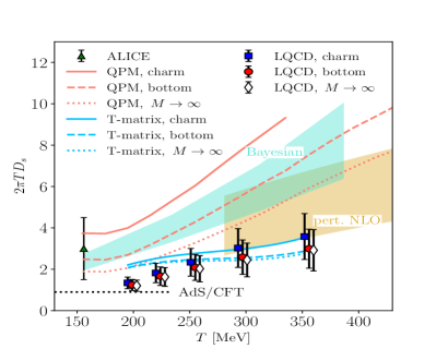
We present the first study of the quark mass dependence of the heavy quark momentum and spatial diffusion coefficients using lattice QCD with light dynamical quarks corresponding to a pion mass of 320 MeV. We find that, for the temperature range 195 MeV 352 MeV, the spatial diffusion coefficients of the charm and bottom quarks are smaller than those obtained in phenomenological models that describe the spectra and elliptic flow of open heavy flavor hadrons.
Introduction.– Heavy-ion experiments at high energies hint toward a rapid thermalization of heavy (charm and bottom) quarks. These observations are surprising since the relaxation time of a heavy quark immersed in a quark-gluon plasma (QGP) is expected to be times larger than the relaxation time of the light bulk degrees of freedom constituting the QGP, where is the heavy quark mass Svetitsky (1988); Moore and Teaney (2005) and is the temperature of the QGP. These experimental observations corroborate the picture that the QGP created in such high-energy heavy-ion collisions is an almost perfect fluid, see Refs. Beraudo et al. (2018); Dong et al. (2019); He et al. (2023). This makes the heavy quark diffusion coefficient one of the fundamental transport properties of the QGP, along with other transport coefficients such as shear and bulk viscosities.
The heavy quark momentum diffusion coefficient is defined as the average momentum transfer squared to a heavy quark from the medium per unit time, and thus characterizes the kinetic relaxation of heavy quarks toward thermal equilibrium. One can also define the spatial heavy quark diffusion coefficient in terms of the conserved net heavy flavor number through the usual Kubo formula. This spatial heavy quark diffusion coefficient will depend on , and also has a well defined limit when goes to zero. Close to equilibrium, in the limit , the momentum and spatial heavy quark diffusion coefficients are related Moore and Teaney (2005); Bouttefeux and Laine (2020),
| (1) |
where is thermal averaged momentum squared of the heavy quark.
Experimentally measured spectra and the elliptic flows of open charm and open bottom hadrons provide information on the degree of thermalization of the heavy quarks in the QGP, see Refs. Beraudo et al. (2018); Dong et al. (2019); He et al. (2023) for reviews. can be estimated by fitting these experimental measurements using phenomenological transport models, see Refs. Beraudo et al. (2018); Dong et al. (2019); He et al. (2023). A key ingredient of these transport models is an effective momentum-dependent heavy-quark diffusion coefficient, which in turn may depend on some effective in-medium cross sections. The appearing in the Kubo formula can be obtained as the zero-momentum limit of this effective diffusion coefficient.
Very recently, has been calculated in 2+1 flavor QCD for infinitely heavy quarks Altenkort et al. (2023a). This QCD result for the infinite-mass limit turns out to be smaller than the phenomenological estimate of for the charm and bottom quarks. This begs the question of whether or not these discrepancies arise solely due to the mass dependence of . In this Letter we address this question by presenting first lattice QCD calculations of the mass-dependent with light dynamical quarks.
Theoretical framework.– For , can be calculated using heavy quark effective theory Casalderrey-Solana and Teaney (2006); Caron-Huot et al. (2009); Bouttefeux and Laine (2020). In this framework is expressed in terms of the correlation function of chromo-electric () and chromo-magnetic () fields connected by fundamental Wilson lines Casalderrey-Solana and Teaney (2006); Caron-Huot et al. (2009); Bouttefeux and Laine (2020).
In this effective theory
| (2) |
where Caron-Huot et al. (2009); Bouttefeux and Laine (2020), are the spectral functions corresponding to the and field correlation functions, and is the mean-squared thermal velocity of the heavy quark Bouttefeux and Laine (2020). The quark mass dependence of enters through . At the leading order in , . In this way, controls the quark mass dependence of .
Lattice QCD calculations of rely on accessing from the correlator Bouttefeux and Laine (2020)
| (3) |
where is the inverse temperature, is the Euclidean time separation of the operators, and is a thermal Wilson line connecting the -fields located at Euclidean times and . is related to via the integral equation
| (4) |
Lattice QCD setup.– In the present calculation we use the same lattice QCD setup and ensembles that were used for the calculation of Altenkort et al. (2023a), specifically, 2+1 flavors of quarks in the Highly Improved Staggered Quark fermionic action Follana et al. (2007) and the tree-level improved Lüscher-Weisz gauge action Luscher and Weisz (1985a, b) with physical values of the kaon and 320 MeV pion masses and at 195, 220, 251, 293 and 352 MeV. At each temperature (except 352 MeV) we use three lattice spacings () to carry out continuum extrapolations () of . Further details are provided in Supplemental Material sup .
The -fields are discretized on the lattice as For measurements of we use a Symanzik-improved version Ramos and Sint (2016) of gradient flow Narayanan and Neuberger (2006); Lüscher (2010, 2010); Lüscher and Weisz (2011). Guided by our experience Altenkort et al. (2021); Brambilla et al. (2023) and perturbative QCD (pQCD) Eller and Moore (2018) we limit the gradient-flow time () within the range . We find that gradient flow improves the signal-to-noise ratio of .
At 1-loop level Eichten and Hill (1990) in pQCD has a nontrivial anomalous dimension, and gradient flow serves as a nonperturbative renormalization scheme for . The continuum-extrapolated are renormalized in the gradient-flow scheme at the scale . The renormalization-group invariant physical correlator, , is obtained via the one-loop pQCD matching Cruz and Moore
| (5) |
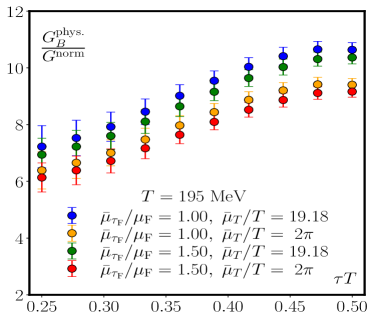
The power-law corrections arising from mixing with high-dimension operators are removed through the extrapolations at each . The matching function, , involves three components: matching from the gradient-flow to the scheme at a scale , matching between -renormalized thermal QCD to the static quark effective theory at a scale , and running of the anomalous dimension of the operator from to . If were known up to all orders in pQCD, the dependence of on the scales and would exactly cancel. Since is known only up to one loop (NLO), we estimate the uncertainty from unknown higher-order effects in the matching by varying the values of each scale; for we consider the two choices or 19.18, and for we consider or 1.4986. Further details and the expression for are given in Supplemental Material sup .
Data analysis.–
The -field correlator scales with a strong negative power of since at large . To mitigate this as well as the lattice artifacts and distortion due to gradient flow Altenkort et al. (2023a) we normalize with , where is the tree-level pQCD results for at nonzero lattice spacing and gradient-flow time, is the Casimir factor, and is the strong coupling. For brevity we suppress the arguments of the normalization correlator.
Our lattice data are not directly, but with the number of points across the lattice time direction, which is related to the lattice spacing via . Therefore, before performing the limit in Eq. (5), we must first take the limit to find . Because the available values also depend on the lattice spacing, we first perform a -interpolation of on the two coarsest lattices, separately at each pair, to establish the value at the values available on the finest lattice. This then allows the extrapolation, which is performed independently at each triple. In extrapolating to we assume that the discretization errors scale as .
For each , to take the limit we multiply the continuum-extrapolated results for by and do linear extrapolations in , as suggested by NLO pQCD Eller (2021). To avoid potentially large discretization effects and to keep the gradient-flow scale smaller than all relevant physical scales in the problem, we restrict to the range of flow times Altenkort et al. (2023a). At MeV we also perform such flow extrapolation based on the single lattice.
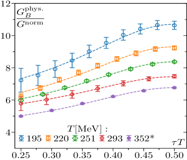
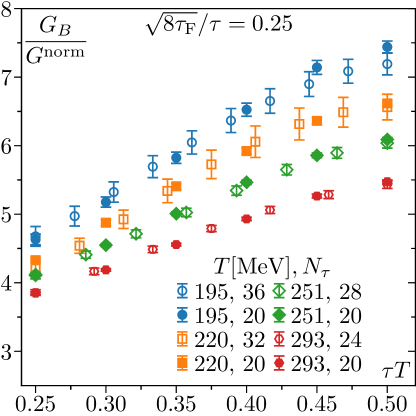
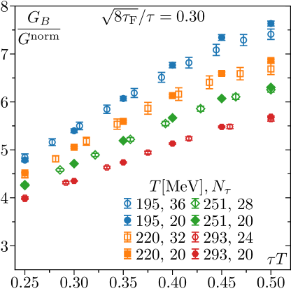
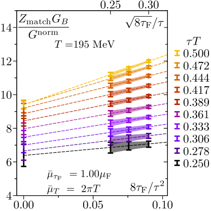
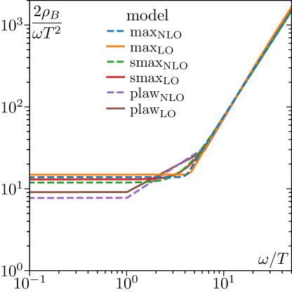
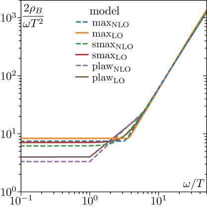
As an example, in Fig. 1 (left panel) we show the resulting for different choices of and . In Fig. 1 (right panel) we show the dependence of for and . Further details on and examples of can be found in Supplemental Material sup .
are fitted to Eq. (4) to obtain . is encoded in the infrared region of the spectral function, . For the ultraviolet region of spectral function, , we use leading order and NLO vacuum pQCD results. To convert the NLO pQCD results Banerjee et al. (2022a); Cruz and Moore from the scheme, at the scale , to the renormalization-group invariant physical scheme we use the matching NLO Wilson coefficient Laine (2021), , to the static quark effective theory. To account for possible higher order effects we also introduce another (in addition to ) -independent fit parameter, . The resulting choices for the UV part of the physical spectral function are . Expressions for , , and are given in the Supplemental Material sup .
Following the previous works Francis et al. (2015); Altenkort et al. (2021); Brambilla et al. (2020); Altenkort et al. (2023a) we use three models to interpolate between and to obtain over all . (1) The maximum () model, , which imposes a hard switch-over between the two regimes. (2) The smooth maximum () model, , which imposes a smooth switch-over. (3) The power-law () model, , which is up to and above . In between, it is connected by a power-law curve . The parameters and are chosen to provide continuity at the boundary. Physically motivated choices of these boundaries are and Altenkort et al. (2023a).
, , and also depend on the intermediate renormalization scale . For reasons discussed in the Supplemental Material sup , we consider two options and , where is a typical thermal scale inferred from the high temperature three dimensional effective theory Kajantie et al. (1997).
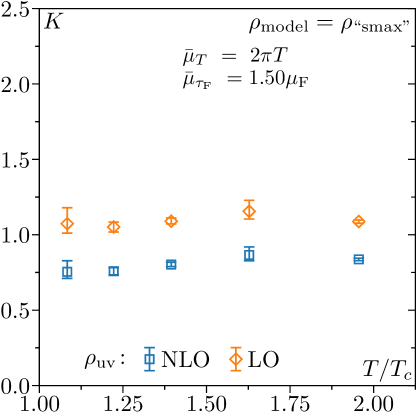
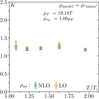
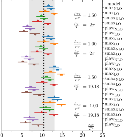
Results.— Combining different choices of (1) and in , (2) and , and (3) three interpolating models , , and , we carry out 24 different fits for and on each bootstrap sample of gauge configurations at each . The final result for at each is obtained from the median and 68% confidence limit of the distribution of all the bootstrap samples over gauge configurations and fit forms and, thus, include both statistical as well as systematic errors arising from different model and scales choices. We find , , , and , which are of similar magnitude to obtained for the same ensembles Altenkort et al. (2023a). The for 2+1 flavor QCD turns out be much larger than those from quenched QCD Banerjee et al. (2022a); Brambilla et al. (2023) at the same values of . For further details on the fits and results see Supplemental Material sup .
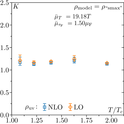
The appearing in Eq. (2) can be obtained either from the low-frequency part of the spectral function corresponding to the net-flavor current Caron-Huot et al. (2009); Burnier and Laine (2012) or in the quasi-particle model with a temperature dependent quark mass Petreczky (2009). In quenched QCD it has been shown that a quasi-particle model with a temperature dependent heavy quark mass fitted to the heavy quark number susceptibility gives a that agrees with the one obtained from the low-frequency part of the net heavy quark current spectral function Petreczky (2009). Therefore, in this work we adopt the quasi-particle model to calculate . For the temperature dependent charm quark is obtained from the continuum-extrapolated lattice QCD results for the charm susceptibility Bellwied et al. (2015). No lattice QCD results for bottom quark susceptibility are available presently. Therefore, we simply fix the effective bottom quark mass to GeV. The needed to obtain , cf. Eq. (1), are estimated from the quasi-particle model in the same way as for the . For further details, see Supplemental Material sup . There we also show that the , and the values of are not too sensitive to the precise choice of the bottom quark mass.
Final results for are summarized in Fig. 2. We find a slight increase in with decreasing heavy quark mass. We compare our results with those obtained from a phenomenological quasi-particle model (QMP) Sambataro et al. (2023) and the T-matrix approach Liu and Rapp (2020); Tang et al. (2023). We find that in QCD is smaller than the results of these calculations and shows smaller dependence on the heavy quark mass, with the exception of the T-matrix result at the highest temperature considered by us. Our result for is also smaller than other phenomenological estimates Xu et al. (2018); Acharya et al. (2022), which do not take into account the quark mass dependence. Finally, for completeness, we show the AdS/CFT estimate Casalderrey-Solana and Teaney (2006) of with a certain value of and the result of the NLO perturbative calculation Caron-Huot and Moore (2008) in the limit .
Conclusion.– We presented the 2+1 flavor lattice QCD calculations of the quark mass dependence of the momentum and spatial heavy quark diffusion coefficients. In the temperature range 195 MeV 352 MeV the quark mass dependence turns out to be quite small. In conjunction with the previous results for an infinitely-heavy quark Altenkort et al. (2023a), the present calculations provide the first non-perturbative QCD results for the charm and bottom quark diffusion coefficients in the QGP. These non-perturbative QCD results will serve as critical inputs to and benchmarks for various dynamical models to study thermalization of charm and bottom quarks in the strongly-coupled medium created in heavy-ion collisions at the Large Hadron Collider and the Relativistic Heavy-Ion Collider.
All computations in this work were performed using SIMULATeQCD Mazur (2021); Bollweg et al. (2022); Mazur et al. (2023).
All data from our calculations, presented in the figures of this paper, can be found in Altenkort et al. (2023b).
Acknowledgments.— This material is based upon work supported by the U.S. Department of Energy, Office of Science, Office of Nuclear Physics through Contract No. DE-SC0012704, and within the frameworks of Scientific Discovery through Advanced Computing (SciDAC) award Fundamental Nuclear Physics at the Exascale and Beyond and the Topical Collaboration in Nuclear Theory Heavy-Flavor Theory (HEFTY) for QCD Matter. This work is supported by the Deutsche Forschungsgemeinschaft (DFG, German Research Foundation) through the CRC-TR 211 “Strong-interaction matter under extreme conditions”– Project No. 315477589 – TRR 211. R. L. acknowledges funding by the Research Council of Norway under the FRIPRO Young Research Talent Grant No. 286883. We thank Szabolcs Borsányi for providing the continuum extrapolated data for charm susceptibility.
This research used awards of computer time provided by: the ALCC program at the Oak Ridge Leadership Computing Facility, which is a DOE Office of Science User Facility supported under Contract No. DE-AC05-00OR22725; the National Energy Research Scientific Computing Center (NERSC), a U.S. Department of Energy Office of Science User Facility located at Lawrence Berkeley National Laboratory, operated under Contract No. DE-AC02- 05CH11231; the PRACE awards on JUWELS at GCS@FZJ, Germany and Marconi100 at CINECA, Italy. Computations for this work were carried out in part on facilities of the USQCD Collaboration, which are funded by the Office of Science of the U.S. Department of Energy. Parts of the computations in this work also were performed at Bielefeld University’s GPU Cluster, supported by HPC.NRW.
References
- Svetitsky (1988) B. Svetitsky, Phys. Rev. D 37, 2484 (1988).
- Moore and Teaney (2005) G. D. Moore and D. Teaney, Phys. Rev. C 71, 064904 (2005), arXiv:hep-ph/0412346 .
- Beraudo et al. (2018) A. Beraudo et al., Nucl. Phys. A 979, 21 (2018), arXiv:1803.03824 [nucl-th] .
- Dong et al. (2019) X. Dong, Y.-J. Lee, and R. Rapp, Ann. Rev. Nucl. Part. Sci. 69, 417 (2019), arXiv:1903.07709 [nucl-ex] .
- He et al. (2023) M. He, H. van Hees, and R. Rapp, Prog. Part. Nucl. Phys. 130, 104020 (2023), arXiv:2204.09299 [hep-ph] .
- Bouttefeux and Laine (2020) A. Bouttefeux and M. Laine, JHEP 12, 150 (2020), arXiv:2010.07316 [hep-ph] .
- Altenkort et al. (2023a) L. Altenkort, O. Kaczmarek, R. Larsen, S. Mukherjee, P. Petreczky, H.-T. Shu, and S. Stendebach (HotQCD), Phys. Rev. Lett. 130, 231902 (2023a), arXiv:2302.08501 [hep-lat] .
- Casalderrey-Solana and Teaney (2006) J. Casalderrey-Solana and D. Teaney, Phys. Rev. D 74, 085012 (2006), arXiv:hep-ph/0605199 .
- Caron-Huot et al. (2009) S. Caron-Huot, M. Laine, and G. D. Moore, JHEP 04, 053 (2009), arXiv:0901.1195 [hep-lat] .
- Follana et al. (2007) E. Follana, Q. Mason, C. Davies, K. Hornbostel, G. P. Lepage, J. Shigemitsu, H. Trottier, and K. Wong (HPQCD, UKQCD), Phys. Rev. D75, 054502 (2007), arXiv:hep-lat/0610092 [hep-lat] .
- Luscher and Weisz (1985a) M. Luscher and P. Weisz, Commun. Math. Phys. 97, 59 (1985a), [Erratum: Commun.Math.Phys. 98, 433 (1985)].
- Luscher and Weisz (1985b) M. Luscher and P. Weisz, Phys. Lett. B 158, 250 (1985b).
- (13) See Supplemental Material for the technical details of this study, which includes Refs. Stendebach (2022); Altenkort et al. (2021, 2023a); Banerjee et al. (2022b, a); Bazavov and Petreczky (2010); Bazavov et al. (2018); Bellwied et al. (2015); Brambilla et al. (2020, 2023); Caron-Huot et al. (2009); Chetyrkin et al. (2000); Clark and Kennedy (2004); Clark et al. (2005); Aoki et al. (2022); Herren and Steinhauser (2018); Bazavov et al. (2014a); Kajantie et al. (1997); Laine (2021); Bazavov et al. (2010); Petreczky (2009); Cruz and Moore .
- Ramos and Sint (2016) A. Ramos and S. Sint, Eur. Phys. J. C 76, 15 (2016), arXiv:1508.05552 [hep-lat] .
- Narayanan and Neuberger (2006) R. Narayanan and H. Neuberger, JHEP 03, 064 (2006), arXiv:hep-th/0601210 [hep-th] .
- Lüscher (2010) M. Lüscher, Commun. Math. Phys. 293, 899 (2010), arXiv:0907.5491 [hep-lat] .
- Lüscher (2010) M. Lüscher, JHEP 08, 071 (2010), [Erratum: JHEP 03, 092 (2014)], arXiv:1006.4518 [hep-lat] .
- Lüscher and Weisz (2011) M. Lüscher and P. Weisz, JHEP 02, 051 (2011), arXiv:1101.0963 [hep-th] .
- Altenkort et al. (2021) L. Altenkort, A. M. Eller, O. Kaczmarek, L. Mazur, G. D. Moore, and H.-T. Shu, Phys. Rev. D 103, 014511 (2021), arXiv:2009.13553 [hep-lat] .
- Brambilla et al. (2023) N. Brambilla, V. Leino, J. Mayer-Steudte, and P. Petreczky (TUMQCD), Phys. Rev. D 107, 054508 (2023), arXiv:2206.02861 [hep-lat] .
- Eller and Moore (2018) A. M. Eller and G. D. Moore, Phys. Rev. D 97, 114507 (2018), arXiv:1802.04562 [hep-lat] .
- Eichten and Hill (1990) E. Eichten and B. R. Hill, Phys. Lett. B 243, 427 (1990).
- (23) D. d. l. Cruz and G. D. Moore, in preparation .
- Sambataro et al. (2023) M. L. Sambataro, V. Minissale, S. Plumari, and V. Greco, (2023), arXiv:2304.02953 [hep-ph] .
- Liu and Rapp (2020) S. Y. F. Liu and R. Rapp, Eur. Phys. J. A 56, 44 (2020), arXiv:1612.09138 [nucl-th] .
- Tang et al. (2023) Z. Tang, S. Mukherjee, P. Petreczky, and R. Rapp, (2023), arXiv:2310.18864 [hep-lat] .
- Xu et al. (2018) Y. Xu, J. E. Bernhard, S. A. Bass, M. Nahrgang, and S. Cao, Phys. Rev. C 97, 014907 (2018), arXiv:1710.00807 [nucl-th] .
- Acharya et al. (2022) S. Acharya et al. (ALICE), JHEP 01, 174 (2022), arXiv:2110.09420 [nucl-ex] .
- Caron-Huot and Moore (2008) S. Caron-Huot and G. D. Moore, Phys. Rev. Lett. 100, 052301 (2008), arXiv:0708.4232 [hep-ph] .
- Eller (2021) A. M. Eller, The Color-Electric Field Correlator under Gradient Flow at next-to-leading Order in Quantum Chromodynamics, Ph.D. thesis, Technische Universität Darmstadt (2021).
- Banerjee et al. (2022a) D. Banerjee, S. Datta, and M. Laine, JHEP 08, 128 (2022a), arXiv:2204.14075 [hep-lat] .
- Laine (2021) M. Laine, JHEP 06, 139 (2021), arXiv:2103.14270 [hep-ph] .
- Francis et al. (2015) A. Francis, O. Kaczmarek, M. Laine, T. Neuhaus, and H. Ohno, Phys. Rev. D 92, 116003 (2015), arXiv:1508.04543 [hep-lat] .
- Brambilla et al. (2020) N. Brambilla, V. Leino, P. Petreczky, and A. Vairo, Phys. Rev. D 102, 074503 (2020), arXiv:2007.10078 [hep-lat] .
- Kajantie et al. (1997) K. Kajantie, M. Laine, K. Rummukainen, and M. E. Shaposhnikov, Nucl. Phys. B 503, 357 (1997), arXiv:hep-ph/9704416 .
- Burnier and Laine (2012) Y. Burnier and M. Laine, JHEP 11, 086 (2012), arXiv:1210.1064 [hep-ph] .
- Petreczky (2009) P. Petreczky, Eur. Phys. J. C 62, 85 (2009), arXiv:0810.0258 [hep-lat] .
- Bellwied et al. (2015) R. Bellwied, S. Borsanyi, Z. Fodor, S. D. Katz, A. Pasztor, C. Ratti, and K. K. Szabo, Phys. Rev. D 92, 114505 (2015), arXiv:1507.04627 [hep-lat] .
- Mazur (2021) L. Mazur, Topological Aspects in Lattice QCD, Ph.D. thesis, Bielefeld U. (2021).
- Bollweg et al. (2022) D. Bollweg, L. Altenkort, D. A. Clarke, O. Kaczmarek, L. Mazur, C. Schmidt, P. Scior, and H.-T. Shu, PoS LATTICE2021, 196 (2022), arXiv:2111.10354 [hep-lat] .
- Mazur et al. (2023) L. Mazur et al. (HotQCD), (2023), arXiv:2306.01098 [hep-lat] .
- Altenkort et al. (2023b) L. Altenkort, D. de la Cruz, O. Kaczmarek, L. R., M. G.D., M. S., P. P., H.-T. Shu, and S. Stendebach, (2023b), 10.4119/unibi/2985523.
- Clark and Kennedy (2004) M. A. Clark and A. D. Kennedy, Nucl. Phys. B Proc. Suppl. 129, 850 (2004), arXiv:hep-lat/0309084 .
- Clark et al. (2005) M. A. Clark, A. D. Kennedy, and Z. Sroczynski, Nucl. Phys. B Proc. Suppl. 140, 835 (2005), arXiv:hep-lat/0409133 .
- Bazavov et al. (2014a) A. Bazavov et al. (HotQCD), Phys. Rev. D 90, 094503 (2014a), arXiv:1407.6387 [hep-lat] .
- Bazavov et al. (2018) A. Bazavov, P. Petreczky, and J. Weber, Phys. Rev. D 97, 014510 (2018), arXiv:1710.05024 [hep-lat] .
- Bazavov et al. (2010) A. Bazavov et al. (MILC), PoS LATTICE2010, 074 (2010), arXiv:1012.0868 [hep-lat] .
- Bazavov and Petreczky (2010) A. Bazavov and P. Petreczky (HotQCD), J. Phys. Conf. Ser. 230, 012014 (2010), arXiv:1005.1131 [hep-lat] .
- Herren and Steinhauser (2018) F. Herren and M. Steinhauser, Comput. Phys. Commun. 224, 333 (2018), arXiv:1703.03751 [hep-ph] .
- Chetyrkin et al. (2000) K. G. Chetyrkin, J. H. Kuhn, and M. Steinhauser, Comput. Phys. Commun. 133, 43 (2000), arXiv:hep-ph/0004189 .
- Aoki et al. (2022) Y. Aoki et al. (Flavour Lattice Averaging Group (FLAG)), Eur. Phys. J. C 82, 869 (2022), arXiv:2111.09849 [hep-lat] .
- Bazavov et al. (2014b) A. Bazavov et al. (HotQCD), Phys. Rev. D90, 094503 (2014b), arXiv:1407.6387 [hep-lat] .
- Stendebach (2022) S. Stendebach, Perturbative analysis of operators under improved gradient flow in lattice QCD, Master’s thesis, Technische Universität Darmstadt (2022).
- Banerjee et al. (2022b) D. Banerjee, R. Gavai, S. Datta, and P. Majumdar, (2022b), arXiv:2206.15471 [hep-ph] .
Supplemental Materials
In these supporting materials we provide the details mentioned in the Letter for the calculation of the finite mass correction to the heavy quark momentum diffusion coefficient via -field correlators. We start with Sec. I by giving additional details to the lattice setup. In Sec. II we describe the calculation of the matching factor . Sec. III is devoted to the discussions on the continuum and flow time extrapolations of the -field correlators. In Sec. IV we detail the modeling of the spectral function. The obtained is compared to other estimates and in Sec. V. We close by checking the dependence of on the thermal charm and bottom quark mass in Sec. VI.
I Lattice setup
| [MeV] | # conf. | |||||
| 195 | 7.570 | 0.01973 | 0.003946 | 64 | 20 | 5899 |
| 7.777 | 0.01601 | 0.003202 | 64 | 24 | 3435 | |
| 8.249 | 0.01011 | 0.002022 | 96 | 36 | 2256 | |
| 220 | 7.704 | 0.01723 | 0.003446 | 64 | 20 | 7923 |
| 7.913 | 0.01400 | 0.002800 | 64 | 24 | 2715 | |
| 8.249 | 0.01011 | 0.002022 | 96 | 32 | 912 | |
| 251 | 7.857 | 0.01479 | 0.002958 | 64 | 20 | 6786 |
| 8.068 | 0.01204 | 0.002408 | 64 | 24 | 5325 | |
| 8.249 | 0.01011 | 0.002022 | 96 | 28 | 1680 | |
| 293 | 8.036 | 0.01241 | 0.002482 | 64 | 20 | 6534 |
| 8.147 | 0.01115 | 0.002230 | 64 | 22 | 9101 | |
| 8.249 | 0.01011 | 0.002022 | 96 | 24 | 688 | |
| 352 | 8.249 | 0.01011 | 0.002022 | 96 | 20 | 2488 |
The gauge configurations in this study were generated using a Rational Hybrid Monte Carlo (RHMC) algorithm Clark and Kennedy (2004); Clark et al. (2005). The configurations are saved after every 10 trajectories with acceptance rate . The dynamical strange quark mass is at its physical value and the light quarks (up/down) are carrying mass , corresponding to the pion mass of MeV. The masses are obtained from the parametrization of the lines of constant physics from Bazavov et al. (2014a). Here we consider four temperatures 195, 220, 251 and 293 MeV. At each temperature three lattices are used to perform the continuum extrapolation. The finest lattices are of size , where and 36. All the finest lattices have the same , corresponding to GeV determined using the -scale Bazavov et al. (2018), with taken from Bazavov et al. (2010). The two coarser lattices are of size , where 20, 22/24, generated with a value that gives the desired temperature, again determined through the scale. The lattice parameters of the ensembles used in this calculation, including the number of gauge configurations are summarized in Tab. 1.
To account for the possible auto-correlation residing in the correlators we estimate the auto-correlation time by analyzing the Polyakov loop at the maximum flow time allowed in this study . The Polyakov loop, as part of the correlator, exhibits stronger auto-correlation than the correlator itself. Thus its auto-correlation can serve as a conservative estimate for the auto-correlation of the correlator. The auto-correlation also becomes stronger at larger flow time. Therefore our strategy of calculating the auto-correlation is robust. The obtained integrated auto-correlation time is in terms of the number of configurations. Then we group the configurations of that size to make independent bins that are passed to the bootstrap analysis afterwards.
When presenting the temperature dependence of the obtained heavy quark momentum diffusion coefficient, it is conventional in the literature to express it in terms of . in the quenched case means the confinement/deconfinement transition temperature. In full QCD it makes more sense to associate with the chiral crossover temperature, which can be determined by locating the peak location of the disconnected chiral susceptibility. A modelling of the peak location of the disconnected chiral susceptibility suggests that Bazavov and Petreczky (2010) for the quark masses used in this study.
II Determination of the matching factor
The matching factor from the -field correlator in the gradient flow scheme to the physical correlator is obtained using a three-step matching procedure. We first match the gradient flow scheme to the scheme at some UV scale Cruz and Moore . Then evolve the -field operators from scale to some thermal scale , and finally match to the physical correlator using the result of Ref. Laine (2021). The matching factor reads Cruz and Moore
| (6) |
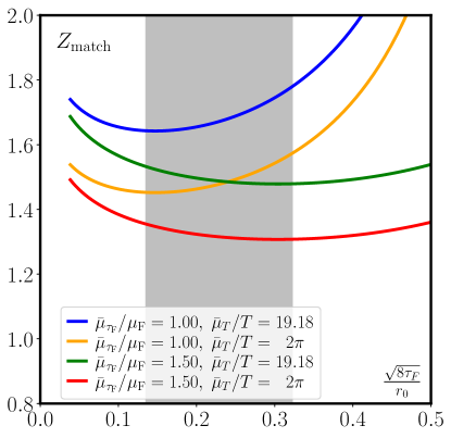
where is the leading-order anomalous dimension of a -field. In the above formula we use coupling constant that is calculated using the RunDec package Herren and Steinhauser (2018); Chetyrkin et al. (2000) with , =0.339 GeV Aoki et al. (2022) at 5-loop. This is justified because at this order the difference between the coupling constant and gradient flow coupling constant can be neglected. Different choices of the scales lead to four different , which are shown as a function of in Fig. 3. fm is taken from Bazavov et al. (2014b). Changing at fixed amounts to an overall multiplicative shift, while changing changes the shape of the curve. However, the small- limiting behavior is not sensitive to . This indicates that the obtained will show a small difference among different choices.
III Continuum and flow time extrapolations
As discussed in the main text, for the analysis of the -field correlator and the continuum extrapolations we need the normalization correlator, . The normalization correlator in the continuum at zero flow time reads Caron-Huot et al. (2009):
| (7) |
Its lattice version at finite flow time is calculated in the same way as for the chromo-electric correlator in Altenkort et al. (2023a) with the difference that the observable matrix here reads Stendebach (2022)
| (8) |
with
| (9) |
After tree level improvement and normalization, which can be done effectively by dividing the the unmatched correlator by the lattice version of the normalized correlator at finite flow time, our results are shown in Fig. 4 at two selected flow times for different temperatures. We show the results for the finest and for the coarsest lattice. We see from the figure that the discretization effects are larger than for the chromo-electric correlator Altenkort et al. (2023a).
To perform the continuum extrapolations the correlators at different lattice spacings are first interpolated using cubic spline to the same separations that are present on the finest lattice. In this way the lattice spacing effects can be seen for each . In Fig. 5 they are shown for some selected s at MeV. One is the lowest and the other is the highest temperature available in this calculation. As an example we pick a fixed relative flow time . As in Ref. Altenkort et al. (2023a) the interpolated correlators are extrapolated to the continuum limit by fitting to the Ansatz in a combined way, assuming that the slope decreases with increasing Altenkort et al. (2023a). Again, it can be seen that, the lattice spacing effects are very minor, similar as in the case of the -field correlators Altenkort et al. (2023a).
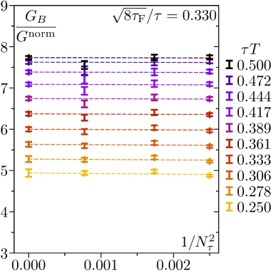
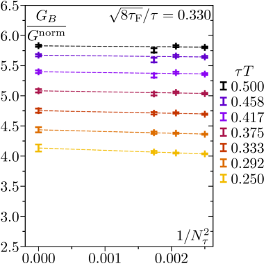
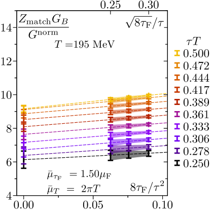
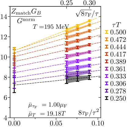
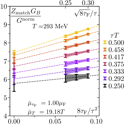
The obtained continuum correlators multiplied by the matching factors are independently extrapolated to the limit linearly in the window . Some of the instances are shown in Fig. 6 for MeV with different and . We see from the figure that the change of changes significantly the slope of the zero flow time extrapolation, while changing effectively amounts to a multiplicative factor in the extrapolated value. In Fig. 6 we also show the zero flow time extrapolation of the normalized -field correlator at MeV. We see that for the same choices of and the slope of the zero flow time extrapolation is somewhat smaller at high temperature.
IV Spectral reconstruction
As discussed in the main text, to obtain from the -field correlators we need to model the spectral function. At high energy the spectral functions can be reliably calculated in perturbation theory. Therefore, we could use the perturbative result to model the high energy part of the spectral function. The spectral function was calculated at NLO in Ref. Banerjee et al. (2022a). Evaluating the NLO contribution numerically we found that the thermal effects are quite small, except at very small values, where perturbation theory is not valid. Therefore, we use the zero temperature limit of the perturbative spectral function in scheme at large :
| (10) | ||||
| (11) |
Here , and . We note that Eq. (10) contains rather than as appears in Ref. Banerjee et al. (2022a) due to a mistake in the original calculation. To obtain the spectral function for the physical scheme we need to multiply the above expressions by for which we use the 1-loop renormaliziation group inspired resummed expression
| (12) |
After multiplying by the scale choice cancels at leading order, but there will be a residual -dependence from higher order contributions. So in practice the choice of has an effect. We consider two choices of . The first choice is , where is the thermal scale of dimensionally reduced effective field theory Kajantie et al. (1997). Our second choice is , which minimizes the NLO contribution for very large . Both choices correspond to a smooth variation of the scale from the natural thermal scale to the frequency in the UV, thus avoiding large logs for large . We also use the above choices of for . is calculated in the same way as it in Eq. (6). To account for the missing higher order effects we multiply the UV part of the spectral function by a constant factor, .
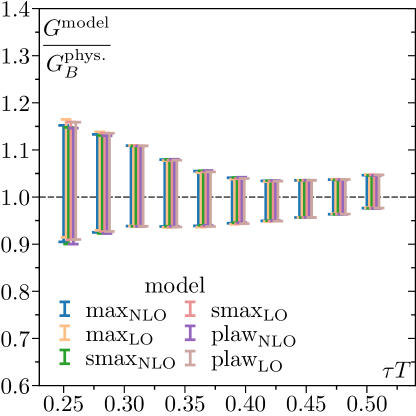
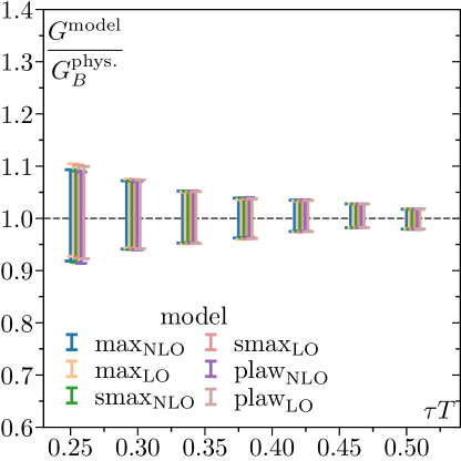
With these choices and definitions we fit the models to our lattice data. All models contain two fit parameters: and . In this section we show fit results using , and as an example. In Fig. 7 we show the fitted spectral functions for the lowest temperature MeV on the left and the highest temperature MeV on the right. It can be seen that using LO or NLO perturbative spectral function makes only a small difference, much smaller than the overall model dependence of the spectral function. This is because beyond the IR scale LO and NLO perturbative spectral function roughly differs by a multiplicative factor, which can be compensated by the adjustment of the -factor in the fitting process, see Fig. 8. The other two temperatures are similar. The ratio of the model correlators and the lattice correlator is shown in Fig. 9, again for MeV and MeV. We can see that the model spectral function describes our lattice data well within errors. The obtained from different models and scales forms a distribution, see Fig. 10. We calculate the weighted average and use it as our final estimate for .


V Comparison of and
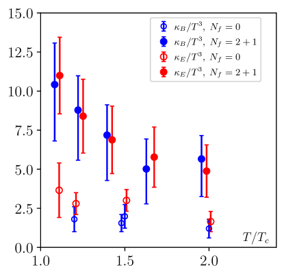
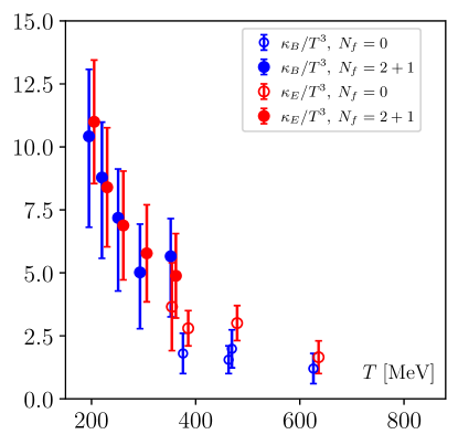
In Fig. 11 we compare and obtained in quenched lattice QCD and -flavor lattice QCD. The quenched are taken from Altenkort et al. (2021); Brambilla et al. (2020); Banerjee et al. (2022b) calculated using gradient flow or multilevel algorithm. The full QCD is taken from Ref. Altenkort et al. (2023a). For quenched we select two estimates, one from multilevel algorithm Banerjee et al. (2022a) and the other from gradient flow at finite Brambilla et al. (2023). We present the figures in terms of both and . One can see that and are of similar size, in both quenched limit and full QCD, when shown in . The full QCD results are much larger at small . When presented in , both and follow a decreasing pattern, connecting smoothly to the quenched results at high temperature.
VI Estimation of and
To obtain and we need to evaluate the averaged velocity squared, , and the averaged momentum squared, of the heavy quark. This can be done assuming that the heavy quarks are well defined quasi particles in the hot medium with a potentially temperature dependent mass, Petreczky (2009). Thus we need to define the masses of the charm and bottom quarks.
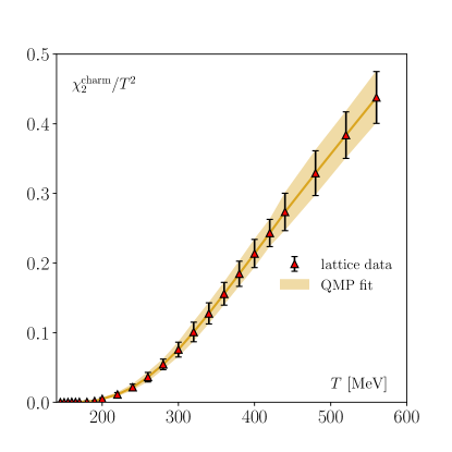
To obtain the charm quark mass, we fit the continuum-extrapolated lattice QCD results of the charm quark number susceptibility Bellwied et al. (2015) to the quasi particle model Petreczky (2009)
| (13) |
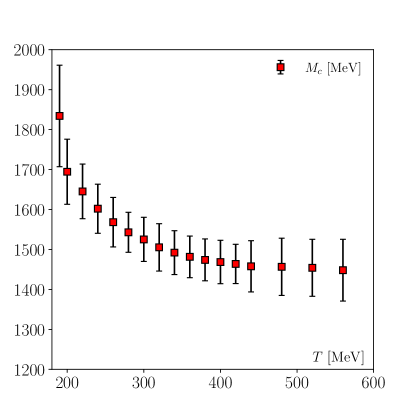
where . Here we use Boltzmann approximation because the heavy quark masses are significantly larger than the temperature. The lattice data of the susceptibility and the fit results are shown in the left panel of Fig. 12 and the extracted charm quark mass is shown in the right panel. It can be seen that the quasi particle model describes the lattice data rather well. We also see that the temperature variation of the charm quark mass between MeV and MeV is 309 MeV. Then the mass is interpolated to the desired temperatures, listed in Table 2. In the table we indicate the uncertainty of the charm masses due to the uncertainties in .
With the extracted mass, and can be calculated again in quasi-particle model Petreczky (2009):
| (14) |
In Table 2 we show , and for charm quarks. Note that the uncertainties in these quantities due to the uncertainty of are small.
We consider two values 4.5 GeV and 4.8 GeV for the bottom quark. The difference between these two values of the bottom quark mass should cover possible thermal effects, see above. In Table 2 we also show , and for bottom quarks. Again the effects of the choice of are small.
| [MeV] | [GeV] | |||||||
|---|---|---|---|---|---|---|---|---|
| 195 | 23.08 | 0.117 | 1.112 | 1.242(267) | 1.74(12) | 0.264(15) | 1.303(23) | 1.338(279)(12) |
| 24.62 | 0.111 | 1.105 | 1.240(267) | |||||
| 220 | 20.45 | 0.131 | 1.127 | 1.671(451) | 1.65(7) | 0.302(9) | 1.364(16) | 1.817(468)(11) |
| 21.82 | 0.124 | 1.118 | 1.666(450) | |||||
| 251 | 17.93 | 0.147 | 1.145 | 2.093(627) | 1.58(5) | 0.342(8) | 1.438(16) | 2.335(671)(14) |
| 19.12 | 0.139 | 1.136 | 2.088(626) | |||||
| 293 | 15.35 | 0.168 | 1.170 | 2.598(835) | 1.53(5) | 0.390(9) | 1.536(19) | 3.026(938)(22) |
| 16.38 | 0.159 | 1.159 | 2.584(831) | |||||
| 352 | 12.78 | 0.197 | 1.206 | 3.004(947) | 1.49(5) | 0.448(9) | 1.677(23) | 3.581(1108)(27) |
| 13.64 | 0.186 | 1.193 | 2.993(946) |