slick: Modeling a Universe of Molecular Line Luminosities in Hydrodynamical Simulations

Abstract

We present slick (the Scalable Line Intensity Computation Kit), a software package that calculates realistic CO, [C I], and [C II] luminosities for clouds and galaxies formed in hydrodynamic simulations. Built on the radiative transfer code despotic, slick computes the thermal, radiative, and statistical equilibrium in concentric zones of model clouds, based on their physical properties and individual environments. We validate our results applying slick to the high-resolution run of the Simba simulations, testing the derived luminosities against empirical and theoretical/analytic relations. To simulate the line emission from a universe of emitting clouds, we have incorporated random forest machine learning (ML) methods into our approach, allowing us to predict cosmologically evolving properties of CO, [C I] and [C II] emission from galaxies such as luminosity functions. We tested this model in 100,000 gas particles, and 2,500 galaxies, reaching an average accuracy of $\sim$99.8% for all lines. Finally, we present the first model light cones created with realistic and ML-predicted CO, [C I], and [C II] luminosities in cosmological hydrodynamical simulations, from $z=0$ to $z=10$.

1 Introduction

Star formation occurs within giant molecular clouds (GMCs), which are mostly composed of molecular hydrogen (H₂). However, H₂ is challenging to observe directly for multiple reasons. First, H₂ lacks a permanent dipole moment, resulting in weak radiative transitions. Second, the first excited transition of H₂ is at $\sim$300 K, which is difficult to excite in the typical temperatures of $10-100$ K found in cold, molecular gas (Fukui & Kawamura, 2010; Dobbs & Pringle, 2013; Krumholz, 2014b). This means that one has to use other trace components of molecular gas to infer the amount of H₂ in observed GMCs.

Carbon molecules/atoms such as carbon monoxide, CO, neutral carbon, [C I], and ionized carbon, [C II], are the most abundant after H₂, and they produce relatively strong and easily observable emission lines, which makes them commonly used tracers of molecular gas (e.g. Bolatto et al., 2013; Vizgan et al., 2022a), atomic gas, and the star formation rate (SFR) of galaxies. CO has many strong transitions in the submillimeter (sub-mm) range of the spectrum, and has been observed extensively to understand the chemical and structural evolution of galaxies (e.g. Carilli & Walter, 2013; Hodge & da Cunha, 2020; Kennicutt & Evans, 2012, and references therein). [C I] has been detected routinely (e.g. Bothwell et al., 2017; Popping et al., 2017), as well as ionized carbon [C II] (e.g. Brisbin et al., 2015; Capak et al., 2015; Schaerer et al., 2015; Knudsen et al., 2016; Inoue et al., 2016), which is a strong coolant in star-forming regions, and a common tracer of SFR. Carilli & Walter (2013); Olsen et al. (2017); Tacconi et al. (2018) present compilations of CO, [C I], and [C II] observations.

Beyond serving as tracers for the physical conditions of molecular gas, observations of CO, [C I], and [C II] also have the potential to constrain cosmological and the evolution of astrophysical parameters in unexplored eras (Kovetz et al., 2017; Bernal & Kovetz, 2022). Ongoing and upcoming line intensity mapping (LIM) experiments, such as the CO Mapping Array Project (COMAP, Cleary et al., 2022), the CONCERTO project (The CONCERTO collaboration et al., 2020), the EXperiment for Cryogenic Large-Aperture Intensity Mapping (EXCLAIM, Pullen et al., 2023), the Fred Young Submillimeter Telescope (FYST, Collaboration et al., 2022), the Terahertz Intensity Mapper (TIM, Vieira et al., 2020), and the Tomographic Ionized-carbon Mapping Experiment (TIME, Crites et al., 2014) will make large-scale intensity maps of these lines from different epochs of the universe to study the cosmic evolution.

Many groups have modeled the physics behind CO, [C I], and [C II] emission from galaxies with different levels of complexity in terms of the galaxy formation model, simulation, and luminosity estimation method. Analytical/empirical models (e.g. Dizgah et al., 2022; Yue & Ferrara, 2019; Zhang et al., 2023) provide a straightforward way of making predictions and analyzing the underlying physics of the studied systems, but they typically rely on assumptions based on observations of specific sets of galaxies at low redshifts. Semi-analytic approaches usually combine N-body simulations, galaxy formation models, and radiative transfer methods to infer luminosities (e.g. Lagos et al., 2012; Popping et al., 2014, 2016; Lagache et al., 2018; Popping et al., 2019; Yang et al., 2021). However, semi-analytic models do not directly simulate the fluid properties in galaxies, instead relying on simplified geometries and analytic prescriptions to describe the physical conditions in star-forming gas.

Cosmological hydrodynamic simulations offer an alternative for computing line emission across cosmic time. Cosmological hydrodynamic simulations fall into two categories: zoom-in simulations, and uniform boxes. Zoom-in simulations follow the line emission properties of individual galaxies, cosmologically, at very high-resolution, though constrain the results to one, or a few individual galaxies (e.g. Pallottini et al., 2017b; Bisbas et al., 2017; Pallottini et al., 2017a; Li et al., 2018; Lupi et al., 2020; Pallottini et al., 2022; Bisbas et al., 2022, 2023). On the other hand, uniform boxes provide large samples of galaxies, though typically have relatively poor resolution compared to zoom-ins; hence sub-resolution modeling is necessary. Beyond this, the cost of running radiative-transfer (RT) equations in all gas particles of such large simulation volumes is significant. For this reason, some groups have relied on empirical relations to make luminosity modeling in large hydrodynamical simulation boxes (e.g. Karoumpis et al., 2022; Murmu et al., 2023). Others have combined photoionization models such as cloudy with hydrodynamical simulations to compute the cloud luminosities from cosmological simulations (Olsen et al., 2016, 2017; Olsen et al., 2021; Leung et al., 2020; Vizgan et al., 2022a; Vizgan et al., 2022b).

In this paper, we develop a new, flexible, and multi-scale method to capture the microphysics of star-forming clouds in cosmological hydrodynamic simulations. Our framework models line luminosities using a combination of hydrodynamical simulations and molecular gas modeling based on each gas particle’s local conditions. We follow the sub-resolution modeling developed in Popping et al. (2019), combined with the chemical network by Gong et al. (2017), and the radiative transfer code despotic (Krumholz, 2014a) . We additionally introduce a machine learning (ML) random forest (RF) framework to apply what we learn from modeling a subset of individual clouds/galaxies to entire cosmological volumes in a computationally efficient manner.

This paper is structured as follows. In Section 2, we explain the basics of the hydrodynamical simulations that we use here, our approach to sub-resolution modeling, and how we compute line luminosities. In Section 3, we introduce slick. In Section 4, we demonstrate applications of slick via proof-of-concept applications to the Simba cosmological simulation. In Section 5, we discuss the importance of our method, its limitations, and how one could improve upon it. Finally, in Section 6, we conclude. Throughout this paper, we adopt a flat, cold dark matter cosmology with ${\Omega}_{0}=0.28$, ${\Omega}_{\Lambda}=0.72$, $h=H_{0}/(100$ km s^-1 Mpc${}^{-1})=0.7$, and $\sigma_{8}=0.812$.

2 Modeling line luminosities in cosmological simulations

The main goal of this work is to employ the physical properties of gas particles (or cells) from galaxy evolution simulations in calculating the sub-mm line luminosity of large samples of galaxies. In what follows, we describe our modeling procedure, and in Section 4 we apply it to the Simba cosmological simulation, which is particle-based. However, these methods are general enough that they can be applied to most galaxy evolution models, and adapted for any cosmological hydrodynamical simulation.

First, we describe each gas particle from a hydrodynamical simulation snapshot with a sub-resolution molecular cloud model. The sub-resolution modeling is necessary because current cosmological simulations do not have sufficient resolution to model the internal structures of molecular clouds (though see Feldmann et al., 2023). Moreover, the majority of cosmological simulations cannot cool to the temperatures relevant for the molecular ISM (Crain & van de Voort, 2023). This is because the Jeans mass for molecular clouds ($10^{4}M_{\sun}$ for a $10$ K cloud) is usually much smaller than the mass-resolution of the simulations ($\sim 10^{6}-10^{7}M_{\sun}$). Hence, we need to assume an artificial resolving temperature, and apply sub-resolution modeling. Our sub-resolution model follows the methodology developed by Popping et al. (2019) for semi-analytical galaxy formation models. Here we adapt it to be used in hydrodynamical simulation particles.

We then use despotic to calculate the statistical, chemical, and thermal equilibria and line luminosities emitting from each sub-resolution molecular cloud. Below, we first describe how we calculate the input properties that the molecular clouds require in despotic (density profile, abundances, impinging UV and CR radiation field); then we briefly describe the workings of despotic. Table 1 shows a summary of the parameters used and calculated in our model, including information on how/where we get/derive them. For a more detailed description of the sub-resolution model and despotic we point the reader to Popping et al. (2019) and Krumholz (2014a), respectively.

2.1 Sub-resolution modeling

Each gas particle in a snapshot at redshift $z$, with mass $M_{\rm{C}}$, number density $n_{0}$, and temperature $T_{\rm{C}}$, is directly extracted from the hydrodynamical simulation. $n_{0}$ and $T_{\rm{C}}$ will be recalculated later during the RT iterations in our model as in principle these parameters are unrealistic for cold molecular gas. At first, however, particle radii, $R_{\rm{C}}$, are calculated based on their mass and the external pressure, $P_{\rm{ext}}$, acting upon them. Following Faesi et al. (2018); Narayanan & Krumholz (2017),

$$\frac{R_{\rm{C}}}{\rm{pc}}=\left(\frac{P_{\rm{ext}}/k_{\rm{B}}}{10^{4}\;\rm{cm^{-3}K}}\right)^{-1/4}\left(\frac{M_{\rm{C}}}{290\;\rm{M_{\sun}}}\right)^{1/2},$$ (1)

where $k_{\rm{B}}$ is the Boltzmann constant, and we assume the equation of state,

$$P_{\rm{ext}}=n_{0}\;k_{\rm{B}}\;T_{\rm{C}}.$$ (2)

2.1.1 Density Profile

We divide each cloud into $16$ different concentric zones, and use a power-law density distribution profile. We have confirmed that the results presented here converge with $16$ zones. Yang et al. (2021) found that clouds with a power-law density profile and size determined by the external pressure, enable more accurate constraints on the CO, [C I], and [C II] emission when compared to using a constant, logotropic, or Plummer profiles. The density, $n_{\rm{H}}$, is then given by

$$n_{\rm{H}}(R)=n_{0}\left(\frac{R_{\rm{C}}}{R}\right)^{-\alpha},$$ (3)

where we adopt $\alpha=2$ (Walker et al., 1990).

2.1.2 Chemical Network

The hydrogen and carbon chemistry of each zone is computed using the Gong-Ostriker-Wolfire (GOW) chemical network (Gong et al., 2017) already implemented in despotic. This network was built upon the NL99 network from Nelson & Langer (1999) and Glover & Clark (2012), allowing for predictions in a broader range of physical conditions. It includes eighteen species: H, H₂, H⁺, H${}_{2}^{+}$, H${}_{3}^{+}$, He, He⁺,O,O⁺,C,C⁺, CO, HCO⁺,Si,Si⁺,e,CH_x, and OH_x. Twelve of these species are independently calculated, and the remaining six (H, He, C, O, Si and e) are derived by ensuring the conservation of total nuclei and charge. The gas-phase abundance of He nuclei is fixed, while C, O, and Si abundances are taken to be proportional to the gas-phase metallicity relative to the solar neighborhood. The gas-phase metallicity, dust abundance, and grain-assisted reaction rates vary with the gas metallicity. We refer the reader to Gong et al. (2017) for more details.

In this work, we set the abundances for carbon ($x_{\rm{C}}$), oxygen ($x_{\rm{O}}$), and silicon ($x_{\rm{Si}}$) based on the cloud metallicities and the scaling relations between metallicities and these abundances by Draine (2011). However, it is straightforward to read the abundances directly from the hydrodynamical simulations. We will assess the effectiveness of this approach in a forthcoming paper.

Table 1: Gas particle (cloud) parameters given as input to radiative transfer code

Parameter	Symbol	Value for each cloud	Units
Gas particle’s properties
Redshift	z	from hydro sim.
Mass	$M_{\rm{C}}$	from hydro sim.	$M_{\sun}$
Metallicity	$Z_{\rm{C}}$	from hydro sim.	$Z_{\sun}$
Star formation rate	SFR	from hydro sim.	$M_{\sun}/\rm{yr}$
Radius	$R_{\rm{C}}$	Eq. 1	pc
External pressure	$P_{\rm{ext}}$	Eq. 2	J/cm3
Density profile	$n_{\rm{H}}$	Eq. 3	1/cm3
Radiation field
Ultraviolet radiation field	$\rm{G}_{\rm{UV}}$	Eq. 6	Habing
Cosmic ray radiation field	$\rm{\xi}_{\rm{CR}}$	Eq. 7	Habing
Ionization rate	$q$	$1\times 10^{-17}\times G_{\rm{UV}}$	Habing
Dust properties
Dust-to-metal ratio	DMR	Eq. 8
Dust abundance relative to solar	$Z_{\rm{d}}$	$1\times Z\times\rm{DMR}$
Dust-gas coupling coefficient	$\alpha_{\rm{GD}}$	$3.2\times 10^{-34}\times Z\times\rm{DMR}$	$\text{erg cm}^{3}\text{K}^{-3/2}$
Cross-sections
Cross-section to 10K thermal radiation	$\sigma_{\rm{D10}}$	$2\times 10^{-25}\times Z\times\rm{DMR}$	$\text{cm}^{2}\text{H}^{-1}$
Cross-section to 8-13.6 eV photons	$\sigma_{\rm{DPE}}$	$1\times 10^{-21}\times Z\times\rm{DMR}$	$\text{cm}^{2}\text{H}^{-1}$
Cross-section to ISRF photons	$\sigma_{\rm{DISRF}}$	$3\times 10^{-22}\times Z\times\rm{DMR}$	$\text{cm}^{2}\text{H}^{-1}$
Species abundances
Carbon abundance	$x_{\rm{C}}$	$1.6\times 10^{-4}\times Z$
Oxygen abundance	$x_{\rm{O}}$	$3.2\times 10^{-4}\times Z$
Silicon abundance	$x_{\rm{Si}}$	$1.7\times 10^{-6}\times Z$

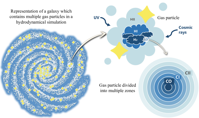
Figure 1: Representation of our model. Gas particle properties and galaxy catalogs come from the hydrodynamical simulations. Each galaxy may contain a few to thousands of gas particles. Gas particle sizes are set as a function of the molecular cloud mass and the external pressure acting on the molecular clouds. They are illuminated by a far-UV radiation field and cosmic rays, based on the gas particles around them. Each gas particle has a radial density profile, and they are radially divided into concentric zones which must achieve chemical, thermal, and statistical equilibrium within our model.

2.1.3 Radiation Field

The radiation field impinging upon molecular clouds, especially the ultraviolet (UV) and cosmic ray (CR) fields, affect the chemistry within the clouds. Popping et al. (2019) showed that [C II] luminosities are more sensitive to the radiation field model than CO and [C I]. This happens because a stronger radiation field ionizes more carbon on the outskirts of the cloud, but it also increases the temperature and optical depth, consequently not affecting much CO and [C I] luminosities. Whereas [C II] only gets stronger with higher temperatures and ionization rates.

There are different approaches to model the strength of UV and CR fields. For instance, Narayanan & Krumholz (2017) scale the strengths with the integrated SFR of galaxies, and Popping et al. (2019) scale them with local SFR surface densities. Here we follow Lagos et al. (2012), and compute a local SFR surface density by summing up the SFRs of the 64 nearest gas particles (the same number of particles that Simba smoothes its mass content over) and dividing it by a cross-sectional area containing these clouds. To account for attenuation, we compute the dust mass density within this cross-sectional area and convert it to a UV optical depth,

$$\tau_{\rm{UV}}=\kappa_{\rm{abs}}\times R_{\rm{\sigma}}\times\frac{3M_{\rm{dust}}}{4\pi R^{3}_{\rm{\sigma}}},$$ (4)

where $\kappa_{\rm{abs}}$ is the mass attenuation coefficient/absorption cross-section per mass of dust, and $R_{\sigma}$ is the radius of the 64-particle sphere. We use $\kappa_{\rm{abs}}=1.078\times 10^{5}\;{\rm{cm}}^{2}{\rm{g}}^{-1}$, which is the median value of the mass attenuation coefficients within the Habing limit of 91.2 nm to 111.0 nm (range at which CO and H₂ photoexcitation and/or photoionization usually occur), assuming a Milky Way (MW) relative variability of $R_{v}=3.1$ .

The Simba cloud neighborhood’s UV transmission probability is then (Lagos et al., 2012):

$$\beta_{\rm{UV}}=\frac{1-e^{-\tau_{\rm{UV}}}}{\tau_{\rm{UV}}}.$$ (5)

This is further normalized by the Solar neighborhood value, which we calculate using a MW gas surface density of $10\;M_{\sun}{\rm{pc}}^{-2}$ (Chang et al., 2002), and a gas-to-dust ratio of 165 ${}^{\ref{drainefootnote}}$, which gives ${\beta}_{\rm{UV,MW}}\approx 0.5$. So the cloud’s UV radiation field is finally

$$\chi=\frac{\Sigma_{\rm{SFR,C}}}{\Sigma_{\rm{SFR,MW}}}\times\frac{\beta_{\rm{UV,C}}}{\beta_{\rm{UV,MW}}},$$ (6)

where ${\Sigma}_{\rm{SFR,C}}$ is the SFR surface density of the cloud, and ${\Sigma}_{\rm{SFR,MW}}$ is the SFR surface density of the Solar neighborhood, equal to $790\;M_{\sun}{\rm{Myr}^{-1}}{\rm{kpc}^{-2}}$ (Bonatto & Bica, 2011).

The CR field is then scaled with the radiation field as

$$\xi_{\rm{CR,C}}=\zeta_{-16}\times\xi_{\rm{CR,MW}}\times\chi,$$ (7)

where $\zeta_{-16}=0.1$ is the CR ionization rate, and $\xi_{\rm{CR,MW}}=10^{-16}s^{-1}$ is the CR field in the Solar neighborhood, both following Narayanan & Krumholz (2017).

2.1.4 Dust Properties

Dust plays an important role in the physics of the ISM; dust grains act as catalysts for the formation of molecules and enable the gas to cool more effectively. Here we highlight the dust property assumptions used in our model.

The cross-sections ($\sigma_{\rm{d,10}}$, $\sigma_{\rm{d,PE}}$, $\sigma_{\rm{d,ISRF}}$), dust abundance ($Z_{\rm{d}}$), and dust-gas coupling coefficient ($\alpha_{\rm{GD}}$) of each cloud are set to scale with the cloud’s dust-to-metal ratio and metallicity, as shown in Table 1. The dust-to-metal ratio, DMR, follows Li et al. (2019) as

$$\rm{DMR}=\frac{\rm{DGR}}{0.44\times Z_{\rm{C}}},$$ (8)

where

$$\log{(\rm{DGR})}=2.445\times\log{\frac{Z_{\rm{C}}}{0.0134}-2.029},$$ (9)

and DGR is the dust-to-gas ratio.

2.2 Computing Line Emission

We use the python package despotic (Krumholz, 2014a) to calculate the spectral line luminosities of the clouds. despotic takes the set of cloud properties described in Subsection 2.1 and Table 1, and simultaneously iterates on the thermal, chemical, and radiative equilibrium equations until convergence is reached in each of the concentric zones. We illustrate this schematically in Fig. 1 and describe the luminosity calculation process in more detail below.

First, despotic assumes statistical equilibrium of the various level populations. The level populations are determined by the balance between the rate of transitions of each species into and out of each level, according to

$$\sum_{j} f_{j}\left[q_{ji}+(1+n_{\gamma,ji})A_{ji}+\frac{g_{i}}{g_{j}}n_{\gamma,ij}A_{ij}\right]$$ (10)

$$=f_{i}\sum_{k}\left[q_{ik}+(1+n_{\gamma,ik})A_{ik}+\frac{g_{k}}{g_{i}}n_{\gamma,ki}A_{ki}\right],$$ (11)

where $f_{i}$ ($f_{j}$) is the fraction of atoms/molecules in the state $i$ ($j$); $A_{ij}$ ($A_{ji}$) is the Einstein coefficient for absorption (emission); and $g_{i}$ ($g_{j}$) represents the degeneracy of the state $i$ ($j$). The parameters

$$n_{\gamma,ij} =\frac{1}{\exp{(\Delta E_{ij}/k_{\rm{B}}T_{\mathrm{CMB}})}-1},$$ (12)

$$q_{ij} =f_{\mathrm{cl}}\;n_{\mathrm{H}}\sum_{p}x_{p}\;k_{p,ij}$$ (13)

are the photon occupation number at the frequency of the line connecting states $i$ and $j$, and the rate of collisional transitions between states $i$ and $j$ summed over all collision partners $p$, respectively. $\Delta E_{ij}$ is the absolute value of the energy emitted/absorbed, $f_{\rm{cl}}$ is a clumping factor, $n_{\rm{H}}$ is the density of the cloud zone, $x_{p}$ is the abundance of species $p$, and $k_{p}$ is the rate coefficient for collisional transitions.

Thermal equilibrium is reached by setting the rate of change of the gas energy per H nucleus equal to zero. The energy rate is

$$\frac{de_{\mathrm{gas}}}{dt}=\Gamma_{\mathrm{ion}}+\Gamma_{\mathrm{PE}}+\Gamma_{\mathrm{grav}}-\Lambda_{\mathrm{line}}+\Psi_{\mathrm{gd}},$$ (14)

where $\Gamma_{\mathrm{ion}}$, $\Gamma_{\mathrm{PE}}$, and $\Gamma_{\mathrm{grav}}$ are the rates of ionization, photoelectric, and gravitational heating per H nucleus, $\Lambda_{\mathrm{line}}$ is the rate of line cooling per H nucleus, and $\Psi_{\mathrm{gd}}$ is the rate of dust-gas energy exchange per H nucleus. despotic then solves for equilibrium gas temperature by setting $de_{\mathrm{gas}}/dt=0$.

Finally, we use despotic to integrate the chemical evolution equations,

$$\frac{d\vec{x}}{dt}=f(\vec{x},n_{\mathrm{H}},N_{\mathrm{H}},T_{\mathrm{g}},\Xi,...),$$ (15)

where $\vec{x}$ is the vector of fractional abundances for the various species taken into account. The reaction rates $d\vec{x}/dt$ can be a function of these abundances, the number density of H, $n_{\mathrm{H}}$, the column density, $N_{\mathrm{H}}$, the gas temperature, $T_{\mathrm{g}}$, the ionization rate, $\Xi$, or any of the other parameters despotic uses to define a cloud. This series of equations is iterated over many times until convergence is reached inside of each zone in each simulation cloud. Finally, the zones are combined to give the full resulting line emission of different species from the cloud.

3 slick: Scalable Line Intensity Computation Kit

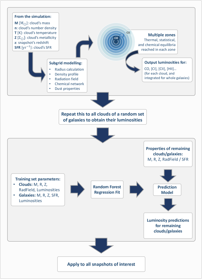
Figure 2: Schematic representation of the steps involved in our exact luminosity calculation + ML modeling. The gas particle mass, number density, temperature, metallicity, redshift, and SFR are extracted directly from the simulation. Cloud radii are calculated using the external pressure, which we calculate based on the cloud number density and mass. The radiation field depends on the neighboring gas particles. For sub-resolution modeling, we assume the initial densities and fractions, a density profile that divides each gas particle in many zones, a chemical network, and the dust properties. All of this information is fed into despotic, which keeps computing abundances until each zone reach thermal, statistical and chemical equilibria, and outputs the luminosities of interest. This is repeated for all gas particles of a given galaxy. One can choose to speed up the process by only running this for certain clouds/galaxies, and using the ML framework to predict luminosities for new clouds/galaxies. A Random Forest model takes clouds’ mass, radius, metallicity and radiation field as input parameters and outputs new predicted luminosities. For galaxies, the input parameters are galaxy mass, radius, metallicity, and SFR. Finally, one can apply this to all snapshots (redshifts) of interest to obtain a light cone.

Obtaining realistic light cones would, at first glance, require that all the processes explained in Section 2 are applied to most (if not all) gas particles in full hydrodynamical simulation snapshots. However, this process of iterating over thermal, chemical, and radiative equilibrium networks for hundreds of millions of gas particles, each divided into many zones, is computationally expensive, and generally unfeasible in reasonable timescales.

In light of this, we here present slick : a framework that makes use of the exact cloud-by-cloud luminosity calculation methods described in Section 2, and offer an additional solution for optimization and scalability of these computations through ML. slick computes both cloud and integrated galaxy realistic luminosities for different molecular lines in snapshots of cosmological hydrodynamical simulations such as Simba (Davé et al., 2019) and IllustrisTNG (Nelson et al., 2015; Pillepich et al., 2018; Donnari et al., 2019).

In detail, slick provides the option to apply the sub-resolution modeling and the radiative transfer equations to all gas particles of a snapshot; or to run them only on a random subset of gas particles, using an RF model to predict luminosities for the remaining ones. slick’s workflow is summarized in Fig. 2. The RF model predicts gas particle luminosities based on their mass, radius, metallicity, and radiation field. We found RF to be the simplest model that can handle complex, non-linear relationships within our data. Besides optimizing the time spent on the luminosity computation within each simulation box, our ML framework also allows for calculation of entire new snapshots if trained on a box with the same resolution and cloud assumptions. For example, one can train the RF on redshifts $z=1$ and $z=2$ and predict the results for $z=1.5$ if the same simulation suite is used for both.

We additionally study the ML mapping of galaxy properties to modeled line emission strengths. In other words, besides gas particle luminosities, our RF model can also predict the integrated line luminosities of galaxies based on their mass, radius, metallicity, SFR, and redshift. This allows us to apply our simulation results to simulations of varying resolutions, and expand the box sizes in future works in this project. We test slick on the Simba simulations, showing its application to Simba 25 Mpc/h boxes, along with validation plots, luminosity functions and light cones in Section 4.

4 slick on Simba

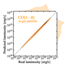
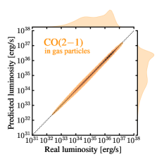
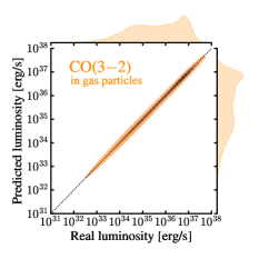
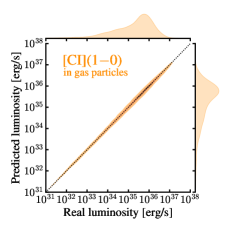
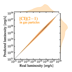
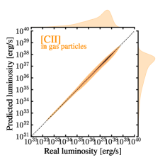
Figure 3: Random Forest Regression model predicts slick’s cloud luminosities with an accuracy of 99.8%. We show kernel density estimation (KDE) plots comparing 30,000 real gas particle luminosities to their predictions using our RF-based ML model. Each plot is for the indicated lines: CO(1-0), CO(2-1), CO(3-2), [C I](1-0), [C I](2-1), and [C II].

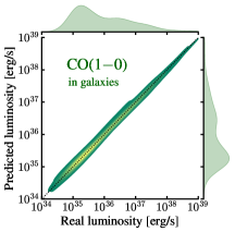
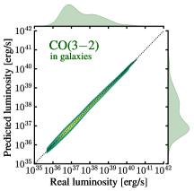
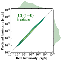
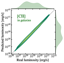
Figure 4: Random Forest Regression model predicts slick’s galaxy luminosities with an accuracy of 99.8%. We show kernel density estimation (KDE) plots to compare 6,000 real galaxy luminosities to their predictions using our RF-based ML model. Each plot is for the indicated lines: CO(1-0), CO(2-1), CO(3-2), [C I](1-0), [C I](2-1), and [C II].

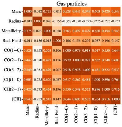
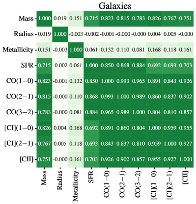
Figure 5: Correlation matrices including our ML model input parameters (which vary depending on the use clouds or galaxies), and some of the lines we can predict. Mass and metallicity are the features which affect the most all cloud line predictions. Mass and SFR are the most important when predictions are for whole galaxies. On the left, a sample of $100,000$ gas particles. On the right, a sample of $2,500$ galaxies.

Simba (Davé et al., 2019) is a suite of galaxy formation simulations developed on the meshless finite mass hydrodynamics of Gizmo (Hopkins, 2015), a code originated from Gadget-3 (Springel et al., 2008). Compared to its predecessor Mufasa, Simba has more realistic sub-resolution prescriptions for star formation, AGN feedback, and black hole growth (Davé et al., 2016). Simba’s outputs consist of snapshots and galaxy catalogs for $151$ redshifts from $z=20$ to $z=0$, for three separate volumes of $25$, $50$, and $100$ Mpc/h per side.

To test our model, we use the highest resolution Simba simulations, which are $25$ Mpc/h-length cubes containing $512^{3}$ particles, with a baryon mass resolution of $1.4\times 10^{6}$ $M_{\sun}$. The cross-matching between galaxies and halo physical properties is found on the caesar catalogs (Thompson, 2014), which identify galaxies using 6-D friends-of-friends, compute galaxy physical properties, and outputs Simba galaxies’ information in a HDF5 catalog. This means that Simba and caesar together provide a mock catalog of clouds, their host galaxies, and their physical properties, such as: mass, number density, temperature, metallicity, etc.

4.1 Validation Tests

4.1.1 ML Model

Figure 6: Our model (slick) matches observational constraints for the $M_{H_{2}}$–$L_{[CO(1-0)]}$ relation. In orange, slick’s $z=0$ galaxy H₂ mass mean (points) and standard deviation (error bars) for different CO(1–0) luminosity bins; in other colors, observational data of extragalactic GMCs, relating their virial masses to their measured luminosities. LMC’s data is from Pineda et al. (2009) and Wong et al. (2011); nearby spirals’ data is from Meyer et al. (2011), Meyer et al. (2013), and Rebolledo et al. (2012); and Local Group’s data is from Bolatto et al. (2008).

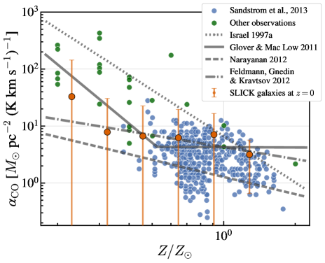
Figure 7: Our model (slick) is in agreement with observational constraints for the relationship between $\alpha_{CO}$ and metallicity, and agrees with other theoretical predictions. In orange, slick’s z = 0 galaxy $\alpha_{CO}$ mean (points) and standard deviation (error bars) for different metallicity bins; while the other colors represent observations of nearby galaxies (Sandstrom et al., 2013; Madden et al., 1997; Leroy et al., 2007; Leroy et al., 2011; Gratier et al., 2010; Roman-Duval et al., 2010; Bolatto et al., 2011; Smith et al., 2012). Bolatto et al. (2013) explains the data in more detail. The solid lines represent a selection of theoretical predictions for this relation (Narayanan et al., 2012; Feldmann et al., 2012; Israel, 1997; Glover & Low, 2011)

.

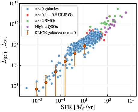
Figure 8: Our model (slick) matches observational constraints for the $L_{[\mathrm{CII}]}$–SFR relation. In orange, slick’s galaxy [C II] luminosity mean (points) and standard deviation (error bars) for different SFR bins; in other colors, observational data from Brauher et al. (2008), Díaz-Santos et al. (2015), Farrah et al. (2013), Graciá-Carpio et al. (2011), Rigopoulou et al. (2014), and Swinbank et al. (2012).

As explained in Section 3, our framework provides an option to predict cloud/galaxy luminosities based on an ML RF model. Figures 3 and 4 demonstrate the performance of our model in predicting the line luminosity of new gas particles, and new galaxies, respectively. We have trained a Random Forest model on 70,000 Simba 25 Mpc/h simulation gas particles randomly picked from the $z=0,1,2,8$, and $10$ snapshots, using their mass, radius, radiation field, metallicity, and redshift as inputs. We tested this model on 30,000 gas particles that were not used in the training. Fig. 3 shows the kernel density estimate (KDE) plot of this distribution. We have also trained this model on full galaxies. Fig. 4 shows the result of 2,000 galaxies training tested on 500 galaxies, using galaxy mass, radius, SFR, metallicity, and redshift as inputs.

The model’s feature importance analysis provides insights into which input parameters are most influential, as highlighted in Fig. 5. When we make predictions for gas particles, all features seem to play an important role, and line luminosities are most sensitive to mass and metallicity. In the case of predictions for whole galaxies, mass and SFR strongly affects all lines, whereas metallicity also plays an important role, especially for [C I] and [C II]. Galaxy radius in our sample is weakly correlated with line luminosities and other physical parameters such as mass, metallicity, and SFR. This is due to the lack of a representative sample of galaxies in terms of their sizes in the 25 Mpc/h box.

4.1.2 Comparison to Observations

We have compared our results to observations and other models in the literature, using the $z=0$ snapshots of the Simba simulations. Following the fluxogram in Fig. 2, we computed CO and [C II] luminosities of half of the $z=0$ gas particles using our sub-resolution model and the radiative transfer code despotic, and the other half using our RF model trained on 70,000 random particles from different snapshots.

First, we compare our simulated galaxy CO(1–0) luminosities and H₂ masses to extragalactic GMC luminosities and virial masses, as shown in Fig. 6. Observational data were extracted from Pineda et al. (2009), Wong et al. (2011), Meyer et al. (2011), Meyer et al. (2013), Rebolledo et al. (2012), and Bolatto et al. (2008). Because the slick predictions are for entire simulated galaxies, whereas observations are of individual GMCs, the mass range covered is not the same. Our least massive galaxies overlap with spiral galaxies and Local Group GMCs, generally presenting a higher molecular mass average for the same $L_{\mathrm{CO}}$ of the observed GMCs. Nevertheless, the general trend in the $M_{\mathrm{H}_{2}}-L_{\mathrm{CO}}$ relation is consistent.

Fig. 7 shows the CO-to-H₂ conversion factor, $\alpha_{\rm{CO}}$ (defined as $\alpha_{\rm{CO}}=M_{\rm{H}_{2}}/L_{\rm{CO}}^{\prime}$) as a function of the mass-weighted metallicity of galaxies. slick’s predictions are compared to observations (Sandstrom et al., 2013; Madden et al., 1997; Leroy et al., 2007; Leroy et al., 2011; Gratier et al., 2010; Roman-Duval et al., 2010; Bolatto et al., 2011; Smith et al., 2012; Israel, 1997; Bolatto et al., 2008; Moustakas et al., 2010) and theoretical predictions(Narayanan et al., 2012; Feldmann et al., 2012; Israel, 1997; Glover & Low, 2011). The high metallicity range of slick’s results agree with most observational data, especially the ones by Sandstrom et al. (2013). On the other hand, some of the observations at lower metallicities yield higher $\alpha_{\mathrm{CO}}$ values than our results. This said, there are significant uncertainties associated with galaxy $\alpha_{\rm{CO}}$ estimation from observations, especially at low metallicities, because they are based on limited empirical calibrations against the metallicity and dust-to-gas ratio.

Fig. 8 shows the relationship between [C II] luminosity and SFR of the $z=0$ snapshot galaxies. For comparison, we included the observational data measurements from Brauher et al. (2008), Díaz-Santos et al. (2015), Farrah et al. (2013), Graciá-Carpio et al. (2011), Rigopoulou et al. (2014), and Swinbank et al. (2012). Our model at $z=0$ is consistent with the observed galaxies at the same redshift. However, it does not capture the higher star formation rates and [C II] luminosities due to the absence of larger structures within the 25 Mpc/h volume. Besides that, our simulated data points show a steeper trend than the one from higher-SFR galaxies. Although consistent with the limited observational dataset in the low-SFR range, this difference could be due to increased contributions to the [C II] luminosity from diffuse atomic gas at low SFRs, which we do not model yet.

4.2 Light cone

We build our light cones based on the code methodology developed in Lovell et al. (2021). Initially, a predefined sky area is assumed, which sets the comoving distance covered by the light cone in each snapshot. Depending on the chosen sky area and the redshift of the snapshot, the simulation volume might be too small to cover the observed area. To address this problem, we choose a random line-of-sight alignment axis, and randomly translate the volume along the plane of the sky direction. Then we stitch each consecutive snapshot along this line-of-sight.

In Fig. 9 we use an area $A=0.5$ deg², and paint CO(1-0) (top panel), [C I](1-0) (middle panel), and [C II] (bottom panel) luminosities on each galaxy. In the current setup, which is intended just for quick visualization, the comoving distance between each snapshot is larger than the size of the 25 Mpc/h box, hence we see some gaps between higher redshifts.

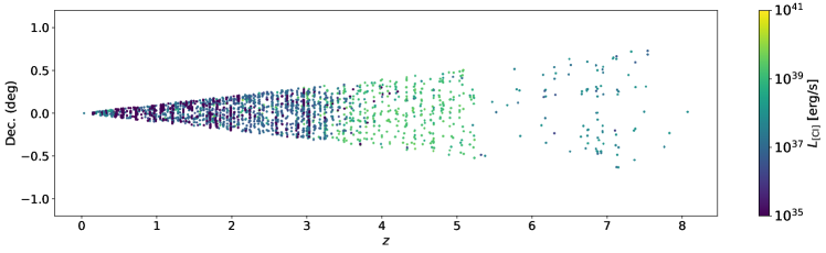
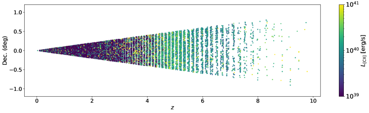
Figure 9: Our combination of RT-based cloud luminosity calculations and ML modeling allows for the construction of entire molecular line light cones. Here we show Simba + slick light cones for CO(1–0) (top), [C I](1–0) (middle), and [C II] (bottom) over 0.5 deg², between 0.1 $\leq$ $z$ $\leq$ 10. Each point represents a galaxy colored by their line luminosities. The x-axis shows the redshift range, and the y-axis shows the declination in degrees.

4.3 Luminosity Functions

We compute CO(1–0) luminosity functions using the full-RT form of slick on all gas particles of the 25 Mpc/h Simba simulation. Fig. 10 shows the CO(1-0) luminosity functions for $z=0,1$, and $2$, where we compare our results to observations and other simulation-based models. $z\sim 0$ observational data is extracted from xCOLD GASS (Saintonge et al., 2017), $z=1$ from ASPECS (Aravena et al., 2019), and $z=2$ COLDz (Pavesi et al., 2018; Riechers et al., 2019). We show Davé et al. (2020)’s luminosity functions in all $z=0,1$, and $2$, where they used the $100$ Mpc/h Simba simulation, but estimated luminosities based on empirical relations. For $z=2$ we also include SIDES simulations by Béthermin et al. (2022), where SFRs and luminosities also come from empirical estimations. Error bars for slick’s data account for sample variance in each luminosity bin. slick’s CO(1-0) luminosity functions are in agreement with the empirical models, and most of the observational data in all redshifts lie within slick’s error bars. Applying slick to larger boxes will allow for more precise measurements at higher luminosities.

Because upcoming [C II] line intensity mapping observations will focus on $z>5$, especially closer to the reionization epoch, we show in Fig. 11 [C II] luminosity functions for redshifts $z=5$ and $z=6$. Different from the full RT calculations for the CO(1-0) luminosity functions, we predict the [C II] line luminosities using our RF model trained on a set of $70,000$ gas particles picked from the $z=0,1,2,8$, and $10$ simulation snapshots. The top panel of Fig. 11 compares slick’s $z=5$ results to ASPECS (Yan et al., 2020; Loiacono et al., 2021) and other $4<z<6$ observations (Swinbank et al., 2012; Capak et al., 2015; Yamaguchi et al., 2017; Cooke et al., 2018). The comparison here is complicated by the fact that the observational data remains sparse, and the 25 Mpc/h box does not contain the large structures required to probe the high luminosity end. However, the overall trend of our results is in agreement with observations. The bottom panel of Fig. 11 shows slick’s $z=6$ results compared to other models in the literature (Lagache et al., 2018; Yue & Ferrara, 2019; Yang et al., 2021; Chung et al., 2020; Béthermin et al., 2022). At $z=6$ the box size limitation is even more prominent; so far slick’s results agree with the other models.

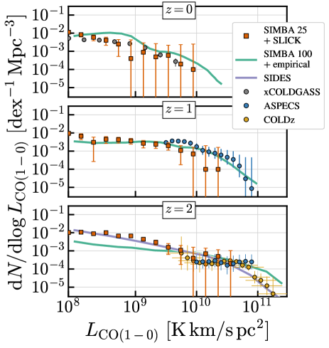
Figure 10: slick’s CO(1-0) luminosity functions in agreement with observations. CO(1–0) luminosity functions at $z=0$, 1, and 2. In orange, results from slick (applied on Simba’s 25 Mpc/h simulation). The green and purple lines refer to simulations using Simba 100 Mpc/h, with luminosities computed using the Narayanan et al. (2012) prescription for $\alpha_{\mathrm{CO}}$, and the SIDES simulations, respectively. The gray, red, and blue circles are observations from xCOLD GASS (Saintonge et al., 2017), ASPECS (Aravena et al., 2019), and COLDz (Riechers et al., 2019). slick reproduces the observational data at $z=0$ and $z=2$ better than Simba and SIDES.

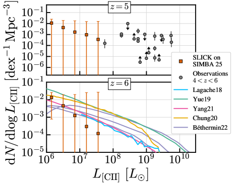
Figure 11: slick’s [C II] luminosity functions for high redshifts puts constraints on low luminosity end predictions. The upper panel shows slick’s ML results for $z=5$, and compares it to ALPINE observations (Yan et al., 2020; Loiacono et al., 2021), and observations by Swinbank et al. (2012); Capak et al. (2015); Yamaguchi et al. (2017); Cooke et al. (2018), all with $4<z<6$. Our current simulation volume does not reach the higher luminosity structures. The lower panel shows slick’s results for $z=6$, which is in agreement within the error bars to other simulations (Lagache et al., 2018; Yue & Ferrara, 2019; Yang et al., 2021; Chung et al., 2020; Béthermin et al., 2022).

5 Discussion

In this work, we have developed the first-ever method that calculates exact CO, [C I], and [C II] luminosities on a cloud-by-cloud basis in full cosmological hydrodynamical simulations, with flexibility to expand to larger boxes through ML. We presented an application of slick to the Simba’s 25 Mpc/h simulation, but we reiterate that this method can be applied to any simulation or galaxy formation model. It has already been used on IllustrisTNG datasets, for which results will come in a forthcoming paper.

From the modeling point of view, there are some limitations in our method that can be explored further in future projects. First, Simba cosmological simulations (as well as many other state-of-the-art cosmological hydrodynamical simulations) enforce some form of a temperature (or pressure) floor in order to maintain a stable multiphase ISM. In our model, this impacts the particle radius that we input to our model to calculate line luminosities. This problem is constrained by the resolution of the simulation, and there is always a trade-off between resolution and achieving cosmological volumes. Our sub-resolution and molecular line modeling of the Simba 25 Mpc/h simulation yields results that align well with observational constraints. To expand the box size, we will adopt solutions such as the ML approach described in Section 3 using full galaxies. We can train the ML model using galaxy luminosities from higher resolution boxes and apply to lower-resolution but higher volume ones.

Another challenge for modeling line emission in simulations such as Simba and IllustrisTNG is to model the radiation field around each gas particle, which is currently not performed on-the-fly. Here, we implemented a varying FUV and cosmic-ray field, depending on gas particles neighbouring each cloud. Our model could be improved through a better understanding of the behavior of CR ionization, and by directly modeling the dust temperature.

LIM experiments require fields of view that can capture enough of the large-scale structure to constrain cosmological parameters. Thus a 25 Mpc/h Simba simulation box is not representative, especially at higher redshifts, as shown in Fig. 11. Running slick in its full radiative transfer form on larger snapshots (such as the 300 Mpc IllustrisTNG) would be unfeasible, and the poorer resolution of such larger boxes could affect the accuracy of our luminosity calculations (although this yet needs to be tested and quantified). The ML approach implemented on slick makes it possible to calculate luminosities in these larger boxes independent of observational empirical relations. However, this process can be improved by using more representative samples of galaxies when training the ML. In a forthcoming paper, we will broaden the training set with larger sets of input simulations.

For LIM experiment forward modeling, cosmic variance will be a challenge. Combining slick with CAMELS (Cosmology and Astrophysics with MachinE Learning Simulations; Villaescusa-Navarro et al., 2021) may provide a solution for that. CAMELS is a suite of N-body and hydrodynamic simulations, generated using thousands of different cosmological and astrophysical parameters. By applying the luminosity prediction model from slick to many different CAMELS snapshots, we plan to reduce sample variance in the measurements, and test the sensitivity of different astrophysical/cosmological parameters. slick’s scalability and flexibility will make it possible to explore a universe of datasets to better forecast future experiments and analyze upcoming ones.

6 Conclusion

In this paper, we introduced slick (the Scalable Line Intensity Computation Kit), a software package that revolutionizes our ability to calculate CO, [C I], and [C II] luminosities for clouds and galaxies within the context of full cosmological hydrodynamical simulations. Our method operates on a cloud-by-cloud basis, and through ML it offers flexibility to extend its application to simulations of varying scales, and even to different galaxy formation models. Leveraging our ML RF model, we have achieved precise predictions of cloud and galaxy luminosities, as substantiated by Fig. 3 and Fig. 4.

We have demonstrated slick’s capabilities by applying it to the Simba 25 Mpc/h simulation. As shown in Fig. 6, slick’s integrated galaxy parameters generally follow the L_CO–H₂ relation derived from GMC observations, and it agrees with observed galaxy data for the $\alpha_{\rm{CO}}$–$Z$ relation (as seen in Fig. 7), especially at metallicities close to solar. Our model underestimates $\alpha_{\rm{CO}}$ when compared to part of the sample of lower metallicity observations, however the sample in this regime is scarce and the estimation of $\alpha_{\mathrm{CO}}$ from observations relies on uncertain assumptions. Furthermore, our results agree with the L_[CII]–SFR relation derived from $z=0$ galaxy observations (Fig. 8). In the regime we probe (SFR $\leq 10$) we find a steeper curve for the L_[CII]–SFR relation compared to observations of high-z high-SFR galaxies. This is consistent with the available low-SFR data. However, this difference could also be due to increasing [C II] emission contribution from diffuse gas in lower-SFRs, which is not modeled in this work.

Our modeled $z=0,1$ and $2$ CO(1–0) luminosity functions agree with observational data and other simulation-based models, with results depicted in Fig. 10. In the case of [C II], we computed luminosity functions for $z=5$ and $6$ with the intent of comparing it not only to observations but also to LIM predictions from the literature. Fig. 11 shows that the box size did not allow us to capture the high luminosity end from higher redshifts, but highlights the potential of our models if applied to larger simulations.

With slick, we now have a quick, simple, and versatile way of combining the ISM details provided by high resolution simulations with the large scale properties from large simulation boxes, allowing for the construction of entire molecular line light cones with cosmological hydrodynamical simulations.

References

- Aravena et al. (2019) Aravena M., et al., 2019, The Astrophysical Journal, 882, 136
- Bernal & Kovetz (2022) Bernal J. L., Kovetz E. D., 2022, The Astronomy and Astrophysics Review, 30, 5
- Bisbas et al. (2017) Bisbas T. G., Dishoeck E. F. v., Papadopoulos P. P., Szűcs L., Bialy S., Zhang Z.-Y., 2017, The Astrophysical Journal, 839, 90
- Bisbas et al. (2022) Bisbas T. G., et al., 2022, The Astrophysical Journal, 934, 115
- Bisbas et al. (2023) Bisbas T. G., van Dishoeck E. F., Hu C.-Y., Schruba A., 2023, Monthly Notices of the Royal Astronomical Society, 519, 729
- Bolatto et al. (2008) Bolatto A. D., Leroy A. K., Rosolowsky E., Walter F., Blitz L., 2008, The Astrophysical Journal, 686, 948
- Bolatto et al. (2011) Bolatto A. D., et al., 2011, The Astrophysical Journal, 741, 12
- Bolatto et al. (2013) Bolatto A. D., Wolfire M., Leroy A. K., 2013, Annual Review of Astronomy and Astrophysics, 51, 207
- Bonatto & Bica (2011) Bonatto C., Bica E., 2011, Monthly Notices of the Royal Astronomical Society, 415, 2827
- Bothwell et al. (2017) Bothwell M. S., et al., 2017, Monthly Notices of the Royal Astronomical Society, 466, 2825
- Brauher et al. (2008) Brauher J. R., Dale D. A., Helou G., 2008, The Astrophysical Journal Supplement Series, 178, 280
- Brisbin et al. (2015) Brisbin D., Ferkinhoff C., Nikola T., Parshley S., Stacey G. J., Spoon H., Hailey-Dunsheath S., Verma A., 2015, The Astrophysical Journal, 799, 13
- Béthermin et al. (2022) Béthermin M., et al., 2022, Astronomy & Astrophysics, 667, A156
- Capak et al. (2015) Capak P. L., et al., 2015, Nature, 522, 455
- Carilli & Walter (2013) Carilli C., Walter F., 2013, Annual Review of Astronomy and Astrophysics, 51, 105
- Chang et al. (2002) Chang R.-X., Shu C.-G., Hou J.-L., 2002, Chinese Journal of Astronomy and Astrophysics, 2, 226
- Chung et al. (2020) Chung D. T., Viero M. P., Church S. E., Wechsler R. H., 2020, The Astrophysical Journal, 892, 51
- Cleary et al. (2022) Cleary K. A., et al., 2022, The Astrophysical Journal, 933, 182
- Collaboration et al. (2022) Collaboration C.-P., et al., 2022, The Astrophysical Journal Supplement Series, 264, 7
- Cooke et al. (2018) Cooke E. A., et al., 2018, The Astrophysical Journal, 861, 100
- Crain & van de Voort (2023) Crain R. A., van de Voort F., 2023, Annual Review of Astronomy and Astrophysics, 61, 473
- Crites et al. (2014) Crites A. T., et al., 2014. Montréal, Quebec, Canada, p. 91531W, doi:10.1117/12.2057207, http://proceedings.spiedigitallibrary.org/proceeding.aspx?doi=10.1117/12.2057207
- Davé et al. (2016) Davé R., Thompson R., Hopkins P. F., 2016, Monthly Notices of the Royal Astronomical Society, 462, 3265
- Davé et al. (2019) Davé R., Anglés-Alcázar D., Narayanan D., Li Q., Rafieferantsoa M. H., Appleby S., 2019, Monthly Notices of the Royal Astronomical Society, 486, 2827
- Davé et al. (2020) Davé R., Crain R. A., Stevens A. R. H., Narayanan D., Saintonge A., Catinella B., Cortese L., 2020, Monthly Notices of the Royal Astronomical Society, 497, 146
- Dizgah et al. (2022) Dizgah A. M., Nikakhtar F., Keating G. K., Castorina E., 2022, Journal of Cosmology and Astroparticle Physics, 2022, 026
- Dobbs & Pringle (2013) Dobbs C. L., Pringle J. E., 2013, Monthly Notices of the Royal Astronomical Society, 432, 653
- Donnari et al. (2019) Donnari M., et al., 2019, Monthly Notices of the Royal Astronomical Society, 485, 4817
- Draine (2011) Draine B. T., 2011, Physics of the Interstellar and Intergalactic Medium. https://ui.adsabs.harvard.edu/abs/2011piim.book.....D
- Díaz-Santos et al. (2015) Díaz-Santos T., et al., 2015, The Astrophysical Journal Letters, 816, L6
- Faesi et al. (2018) Faesi C. M., Lada C. J., Forbrich J., 2018, The Astrophysical Journal, 857, 19
- Farrah et al. (2013) Farrah D., et al., 2013, The Astrophysical Journal, 776, 38
- Feldmann et al. (2012) Feldmann R., Gnedin N. Y., Kravtsov A. V., 2012, The Astrophysical Journal, 758, 127
- Feldmann et al. (2023) Feldmann R., et al., 2023, Monthly Notices of the Royal Astronomical Society, 522, 3831
- Fukui & Kawamura (2010) Fukui Y., Kawamura A., 2010, Annual Review of Astronomy and Astrophysics, 48, 547
- Glover & Clark (2012) Glover S. C. O., Clark P. C., 2012, Monthly Notices of the Royal Astronomical Society, 421, 116
- Glover & Low (2011) Glover S. C. O., Low M.-M. M., 2011, EAS Publications Series, 52, 147
- Gong et al. (2017) Gong M., Ostriker E. C., Wolfire M. G., 2017, The Astrophysical Journal, 843, 38
- Graciá-Carpio et al. (2011) Graciá-Carpio J., et al., 2011, The Astrophysical Journal Letters, 728, L7
- Gratier et al. (2010) Gratier P., Braine J., Rodriguez-Fernandez N. J., Israel F. P., Schuster K. F., Brouillet N., Gardan E., 2010, Astronomy and Astrophysics, 512, A68
- Hodge & da Cunha (2020) Hodge J. A., da Cunha E., 2020, Royal Society Open Science, 7, 200556
- Hopkins (2015) Hopkins P. F., 2015, Monthly Notices of the Royal Astronomical Society, 450, 53
- Inoue et al. (2016) Inoue A. K., et al., 2016, Science, 352, 1559
- Israel (1997) Israel F. P., 1997, H2 and its relation to CO in the LMC and other magellanic irregulars, doi:10.48550/arXiv.astro-ph/9709194, http://arxiv.org/abs/astro-ph/9709194
- Karoumpis et al. (2022) Karoumpis C., Magnelli B., Romano-Díaz E., Haslbauer M., Bertoldi F., 2022, Astronomy & Astrophysics, 659, A12
- Kennicutt & Evans (2012) Kennicutt R. C., Evans N. J., 2012, Annual Review of Astronomy and Astrophysics, 50, 531
- Knudsen et al. (2016) Knudsen K. K., Richard J., Kneib J.-P., Jauzac M., Clément B., Drouart G., Egami E., Lindroos L., 2016, Monthly Notices of the Royal Astronomical Society: Letters, 462, L6
- Kovetz et al. (2017) Kovetz E. D., et al., 2017, arXiv:1709.09066 [astro-ph]
- Krumholz (2014a) Krumholz M. R., 2014a, Monthly Notices of the Royal Astronomical Society, 437, 1662
- Krumholz (2014b) Krumholz M. R., 2014b, Physics Reports, 539, 49
- Lagache et al. (2018) Lagache G., Cousin M., Chatzikos M., 2018, Astronomy & Astrophysics, 609, A130
- Lagos et al. (2012) Lagos C. d. P., Bayet E., Baugh C. M., Lacey C. G., Bell T. A., Fanidakis N., Geach J. E., 2012, Monthly Notices of the Royal Astronomical Society, 426, 2142
- Leroy et al. (2007) Leroy A., Bolatto A., Stanimirovic S., Mizuno N., Israel F., Bot C., 2007, The Astrophysical Journal, 658, 1027
- Leroy et al. (2011) Leroy A. K., et al., 2011, The Astrophysical Journal, 737, 12
- Leung et al. (2020) Leung T. K. D., Olsen K. P., Somerville R. S., Davé R., Greve T. R., Hayward C. C., Narayanan D., Popping G., 2020, The Astrophysical Journal, 905, 102
- Li et al. (2018) Li Q., Narayanan D., Davè R., Krumholz M. R., 2018, The Astrophysical Journal, 869, 73
- Li et al. (2019) Li Q., Narayanan D., Davé R., 2019, Monthly Notices of the Royal Astronomical Society, 490, 1425
- Loiacono et al. (2021) Loiacono F., et al., 2021, Astronomy & Astrophysics, 646, A76
- Lovell et al. (2021) Lovell C. C., Geach J. E., Davé R., Narayanan D., Li Q., 2021, Monthly Notices of the Royal Astronomical Society, 502, 772
- Lupi et al. (2020) Lupi A., Pallottini A., Ferrara A., Bovino S., Carniani S., Vallini L., 2020, Monthly Notices of the Royal Astronomical Society, 496, 5160
- Madden et al. (1997) Madden S. C., Poglitsch A., Geis N., Stacey G. J., Townes C. H., 1997, The Astrophysical Journal, 483, 200
- Meyer et al. (2011) Meyer J. D., et al., 2011, The Astrophysical Journal, 744, 42
- Meyer et al. (2013) Meyer J. D., et al., 2013, The Astrophysical Journal, 772, 107
- Moustakas et al. (2010) Moustakas J., Kennicutt R. C. J., Tremonti C. A., Dale D. A., Smith J. D. T., Calzetti D., 2010, VizieR Online Data Catalog, p. J/ApJS/190/233
- Murmu et al. (2023) Murmu C. S., et al., 2023, Monthly Notices of the Royal Astronomical Society, 518, 3074
- Narayanan & Krumholz (2017) Narayanan D., Krumholz M. R., 2017, Monthly Notices of the Royal Astronomical Society, 467, 50
- Narayanan et al. (2012) Narayanan D., Krumholz M. R., Ostriker E. C., Hernquist L., 2012, Monthly Notices of the Royal Astronomical Society, 421, 3127
- Nelson & Langer (1999) Nelson R. P., Langer W. D., 1999, The Astrophysical Journal, 524, 923
- Nelson et al. (2015) Nelson D., et al., 2015, Astronomy and Computing, 13, 12
- Olsen et al. (2016) Olsen K. P., Greve T. R., Brinch C., Sommer-Larsen J., Rasmussen J., Toft S., Zirm A., 2016, Monthly Notices of the Royal Astronomical Society, 457, 3306
- Olsen et al. (2017) Olsen K., Greve T. R., Narayanan D., Thompson R., Davé R., Rios L. N., Stawinski S., 2017, The Astrophysical Journal, 846, 105
- Olsen et al. (2021) Olsen K. P., et al., 2021, The Astrophysical Journal, 922, 88
- Pallottini et al. (2017a) Pallottini A., Ferrara A., Gallerani S., Vallini L., Maiolino R., Salvadori S., 2017a, Monthly Notices of the Royal Astronomical Society, 465, 2540
- Pallottini et al. (2017b) Pallottini A., Ferrara A., Bovino S., Vallini L., Gallerani S., Maiolino R., Salvadori S., 2017b, Monthly Notices of the Royal Astronomical Society, 471, 4128
- Pallottini et al. (2022) Pallottini A., et al., 2022, Monthly Notices of the Royal Astronomical Society, 513, 5621
- Pavesi et al. (2018) Pavesi R., et al., 2018, The Astrophysical Journal, 864, 49
- Pillepich et al. (2018) Pillepich A., et al., 2018, Monthly Notices of the Royal Astronomical Society, 475, 648
- Pineda et al. (2009) Pineda J. L., Ott J., Klein U., Wong T., Muller E., Hughes A., 2009, The Astrophysical Journal, 703, 736
- Popping et al. (2014) Popping G., Pérez-Beaupuits J. P., Spaans M., Trager S. C., Somerville R. S., 2014, Monthly Notices of the Royal Astronomical Society, 444, 1301
- Popping et al. (2016) Popping G., van Kampen E., Decarli R., Spaans M., Somerville R. S., Trager S. C., 2016, Monthly Notices of the Royal Astronomical Society, 461, 93
- Popping et al. (2017) Popping G., et al., 2017, Astronomy & Astrophysics, 602, A11
- Popping et al. (2019) Popping G., Narayanan D., Somerville R. S., Faisst A. L., Krumholz M. R., 2019, Monthly Notices of the Royal Astronomical Society, 482, 4906
- Pullen et al. (2023) Pullen A. R., et al., 2023, Monthly Notices of the Royal Astronomical Society, 521, 6124
- Rebolledo et al. (2012) Rebolledo D., Wong T., Leroy A., Koda J., Meyer J. D., 2012, The Astrophysical Journal, 757, 155
- Riechers et al. (2019) Riechers D. A., et al., 2019, The Astrophysical Journal, 872, 7
- Rigopoulou et al. (2014) Rigopoulou D., et al., 2014, The Astrophysical Journal Letters, 781, L15
- Roman-Duval et al. (2010) Roman-Duval J., Jackson J. M., Heyer M., Rathborne J., Simon R., 2010, The Astrophysical Journal, 723, 492
- Saintonge et al. (2017) Saintonge A., et al., 2017, The Astrophysical Journal Supplement Series, 233, 22
- Sandstrom et al. (2013) Sandstrom K. M., et al., 2013, The Astrophysical Journal, 777, 5
- Schaerer et al. (2015) Schaerer D., et al., 2015, Astronomy & Astrophysics, 576, L2
- Smith et al. (2012) Smith M. W. L., et al., 2012, The Astrophysical Journal, 756, 40
- Springel et al. (2008) Springel V., et al., 2008, Monthly Notices of the Royal Astronomical Society, 391, 1685
- Swinbank et al. (2012) Swinbank A. M., et al., 2012, Monthly Notices of the Royal Astronomical Society, 427, 1066
- Tacconi et al. (2018) Tacconi L. J., et al., 2018, The Astrophysical Journal, 853, 179
- The CONCERTO collaboration et al. (2020) The CONCERTO collaboration et al., 2020, Astronomy & Astrophysics, 642, A60
- Thompson (2014) Thompson R., 2014, Astrophysics Source Code Library, p. ascl:1411.001
- Vieira et al. (2020) Vieira J., et al., 2020, The Terahertz Intensity Mapper (TIM): a Next-Generation Experiment for Galaxy Evolution Studies, doi:10.48550/arXiv.2009.14340, http://arxiv.org/abs/2009.14340
- Villaescusa-Navarro et al. (2021) Villaescusa-Navarro F., et al., 2021, The Astrophysical Journal, 915, 71
- Vizgan et al. (2022a) Vizgan D., et al., 2022a, The Astrophysical Journal, 929, 92
- Vizgan et al. (2022b) Vizgan D., Heintz K. E., Greve T. R., Narayanan D., Davé R., Olsen K. P., Popping G., Watson D., 2022b, The Astrophysical Journal Letters, 939, L1
- Walker et al. (1990) Walker C. K., Adams F. C., Lada C. J., 1990, The Astrophysical Journal, 349, 515
- Wong et al. (2011) Wong T., et al., 2011, The Astrophysical Journal Supplement Series, 197, 16
- Yamaguchi et al. (2017) Yamaguchi Y., et al., 2017, The Astrophysical Journal, 845, 108
- Yan et al. (2020) Yan L., et al., 2020, The Astrophysical Journal, 905, 147
- Yang et al. (2021) Yang S., Somerville R. S., Pullen A. R., Popping G., Breysse P. C., Maniyar A. S., 2021, The Astrophysical Journal, 911, 132
- Yue & Ferrara (2019) Yue B., Ferrara A., 2019, Monthly Notices of the Royal Astronomical Society, 490, 1928
- Zhang et al. (2023) Zhang M., Ferrara A., Yue B., 2023, The power spectrum of extended [C II] halos around high redshift galaxies, doi:10.48550/arXiv.2304.07023, http://arxiv.org/abs/2304.07023