Gauge preheating with full general relativity

Abstract

We study gauge preheating following pseudoscalar-driven inflation in full general relativity. We implement the Baumgarte-Shapiro-Shibata-Nakamura (BSSN) scheme to solve the full nonlinear evolution of the metric alongside the dynamics of the pseudoscalar and gauge fields. The dynamics of the background and emission of gravitational waves are broadly consistent with simulations in a Friedmann-Lemaître-Robertson-Walker (FLRW) spacetime. We find large, localized overdensities in the BSSN simulations of order $\delta=\delta\rho/\rho\sim 30$, and the dimensionless power spectrum of $\delta$ peaks above unity. These overdense regions are seeded on length scales only slightly smaller than the horizon, and have a compactness $C\sim 0.1$. The scale of peak compactness is shorter than the Jeans length, which implies that pressure of the matter fields plays an important role in the evolution of these objects.
Date:

1 Introduction

The end of cosmic inflation [1, 2, 3, 4] and the subsequent transition to the radiation-dominated hot Big Bang remains one of the most poorly understood epochs in the evolution of the Universe. During this reheating epoch, the accelerated expansion of inflation must end, and the inflaton energy density must be eventually transferred to relativistic degrees of freedom to begin the hot Big Bang. Because the scales involved are so small—smaller than the Hubble radius at the end of inflation—information about the reheating epoch is either erased as the resulting Standard Model plasma achieves thermal equilibrium or is inseparable from the effects of the subsequent nonlinear gravitational evolution of structure formation.

While reheating may be facilitated by perturbative decays of the inflaton to other particles [5, 6], the homogeneous, oscillating inflaton background can source explosive production of particles and rapid growth of matter inhomogeneities via preheating [7, 8, 9, 10]. The collective dynamics of the oscillating background has long been a fertile ground for model building and searches for observable signatures of reheating [11, 12, 13, 14, 15, 16, 17] (for a review, see Ref. [18]). Possible gravitational relics, such as gravitational waves [19, 20, 21, 22, 23, 24, 25, 26], collapsed structures like primordial black holes [14, 27, 28, 29, 30], or compact mini halos [31, 32], offer potential probes into the reheating epoch.

Preheating into gauge fields—gauge preheating—is an extremely violent process. In models of gauge preheating, effectively all of the energy stored in the inflaton can be transferred into gauge field radiation within a single oscillation of the inflaton about the minima of its potential [33, 34, 35, 36, 37, 38, 39]. This rapid energy transfer is facilitated by a tachyonic instability in the gauge field sourced by the rolling inflaton field. The tachyonic enhancement of gauge fields by rolling pseudoscalars (a long-appreciated phenomenon [40, 41, 42]) can also realize strong backreaction on the homogeneous motion of the pseudoscalar, enabling models of inflation on steep potentials [46, 47] and warm inflation [48]. Away from the regime of strong backreaction, perturbative backreaction of the gauge modes during and after inflation may produce observable non-Gaussianity [49, 50, 51, 52], chiral gravitational waves [53, 54, 53, 52, 55, 56, 57, 58, 59], primordial black holes [60, 61], and primordial magnetic fields [41, 42, 36] and the baryon asymmetry [62, 63, 64, 65, 59, 66, 67, 68].

The strongest effects of gauge field production occur when the inflaton rolls the fastest, which typically occurs at the end of inflation. The large couplings required to produce effects observable on scales accessible to the cosmic microwave background (CMB) or gravitational-wave interferometers subsequently generate a high-frequency gravitational wave background during preheating so large that existing bounds on the effective number of relativistic species rules the regime out [69, 70, 71]. The production of large metric perturbations calls into question whether nonlinear gravitational effects can be safely neglected. Since gravitational wave backgrounds from gauge preheating currently provide the strongest constraint on these models, it is crucial to test the robustness of prior predictions [69, 71, 70] and whether nonlinear gravity might enhance [78] or suppress [79] the production of gravitational waves. Further, the production of large metric fluctuations indicates the presence of large inhomogeneities in the matter sector which may undergo gravitational collapse under the influence of local gravity. The purpose of this work is to push further the exploration of gravitational signatures of preheating into the regime of local, nonlinear gravity. To that end, building on the results of [80], we initiate a study of preheating into gauge fields using the full machinery of numerical relativity [81, 82, 83] to follow the nonlinear evolution of the metric.

In this paper, we demonstrate that preheating probes regions where nonlinear gravitational effects are expected to become important, and we explore the degree to which simulations that include nonlinear gravity are required to accurately characterize this epoch. In particular, we perform a careful study of gravitational effects during gauge preheating, focusing on the development of large density inhomogeneities and gravitational wave production. We first demonstrate that linearized gravity is quickly violated. Then, using numerical relativity, we follow the evolution of the metric including the effects of dynamical gravity to show that this breakdown of linearized gravity does not signal the formation of black holes. We demonstrate that, despite producing regions with very large density contrasts $\delta\rho/\rho\sim 30$, there is nevertheless no evidence that black holes are formed—no horizons are formed in our simulations. We show that the spatial extent of the regions of large density contrast are smaller than the Jeans length, which indicates that pressure plays an important role in their subsequent evolution. Furthermore, their compactness, which is a measure of whether a region satisfies the so-called ‘hoop-conjecture’ [84], attains a maximum value of $C\sim 10^{-1}$.

The paper is structured as follows. In section 2 we define the model and present the equations that govern the evolution and amplification of gauge fields during and after inflation. In section 3 we present results of numerical simulations, focusing on the dynamics of density and gravitational wave fluctuations as a function of the axion-gauge coupling strength. Our conclusions and proposed avenues for future work are presented in section 4. The details of the decomposition of gauge fields in the BSSN formalism are relegated to appendix A, while appendix B details how our initial conditions are set in perturbation theory in the BSSN formalism, and finally appendix C describes robustness checks of our results.

We use natural units, which set $\hbar=c=1$, and define the reduced Planck mass $M_{\mathrm{Pl}}=1/\sqrt{8\pi G}$. Repeated/contracted Greek spacetime indices are summed via the Einstein summation convention.

2 Gauge preheating and the BSSN formalism

We consider a pseudoscalar inflaton, $\varphi$, minimally coupled to Einstein gravity, and coupled to a U(1) gauge field, $A_{\mu}$, described by the action

$$S =\int\mathrm{d}^{4}x\,\sqrt{-g}\left[\frac{M_{\mathrm{Pl}}^{2}}{2}R-\frac{1}{2}\nabla_{\mu}\varphi\nabla^{\mu}\varphi-V(\varphi)-\frac{1}{4}F_{\mu\nu}F^{\mu\nu}-\frac{X(\varphi)}{4}F_{\mu\nu}\tilde{F}^{\mu\nu}\right].$$ (2.1)

where $R$ is the Ricci scalar and $F_{\mu\nu}=\nabla_{\mu}A_{\nu}-\nabla_{\nu}A_{\mu}$ is the field strength tensor whose dual is

$$\tilde{F}^{\mu\nu}=\frac{1}{2}\epsilon^{\mu\nu\alpha\beta}F_{\alpha\beta}.$$ (2.2)

The Levi-Civita tensor is

$$\epsilon_{\mu_{1}\mu_{2}\cdots\mu_{n}}=\sqrt{-g}\varepsilon_{\mu_{1}\mu_{2}\cdots\mu_{n}},$$ (2.3)

which is written in terms of the permutation symbol (the Levi-Civita symbol), $\varepsilon_{\mu_{1}\mu_{2}\cdots\mu_{n}}$. We work with the convention that $\epsilon^{\mu_{1}\mu_{2}\cdots\mu_{n}}\equiv\mathrm{sign}\,g\,\varepsilon^{\mu_{1}\mu_{2}\cdots\mu_{n}}/\sqrt{-g}$, such that $\varepsilon^{\mu_{1}\mu_{2}\cdots\mu_{n}}\equiv\varepsilon_{\mu_{1}\mu_{2}\cdots\mu_{n}}$. Here $\nabla_{\mu}$ denotes the ($\mu$ component of) the four dimensional covariant derivative compatible with the full metric $g_{\mu\nu}$.

We consider a simple toy model of inflation specified by the potential [2]

$$V=\frac{1}{2}m^{2}\varphi^{2}.$$ (2.4)

Planck’s best-fit scalar spectral amplitude $A_{s}\approx 2.1\times 10^{-9}$ [85] sets $m=6.05\times 10^{-6}\,M_{\mathrm{Pl}}$. Though inflation driven by a monomial potential is strongly disfavored [86, 87], we choose a quadratic potential merely to provide a simple model for the inflaton’s dynamics during preheating. For further discussion of the effects of potential choice on gauge preheating, see [70]. We consider the standard shift-symmetric, dimension-5 axial coupling between the pseudoscalar and the gauge field

$$X(\varphi) =\frac{\alpha_{g}}{M_{\mathrm{Pl}}}\varphi.$$ (2.5)

Numerical investigations of preheating typically employ a homogeneously expanding, Friedmann-Lemaître-Robertson-Walker (FLRW) background spacetime with metric

$$g_{\mu\nu}^{\rm FLRW} =a(\tau)^{2}\eta_{\mu\nu}=a(\tau)^{2}\operatorname{diag}\left[-1,1,1,1\right].$$ (2.6)

Here $\tau$ is conformal time, and the scale factor $a(\tau)$ evolves according to the Friedmann equations

$$\mathcal{H}^{2}\equiv\left(\frac{{a^{\prime}}}{a}\right)^{2}=\frac{a^{2}}{3M_{\mathrm{Pl}}^{2}}\bar{\rho}\,,$$ (2.7)

and

$$\mathcal{H}^{\prime}+\mathcal{H}^{2}=\frac{a^{2}}{6M_{\mathrm{Pl}}^{2}}\left(\bar{\rho}-3\bar{P}\right).$$ (2.8)

Primes denote a derivative with respect to conformal time, $\tau$, and overbars generally indicate averaged quantities on constant-$\tau$ hypersurfaces. The (averaged) energy density and pressure are $\bar{\rho}\equiv-\bar{T}^{0}_{\hphantom{0}0}$ and $\bar{P}\equiv\delta_{i}^{\hphantom{i}j}\bar{T}^{i}_{\hphantom{i}j}/3$, respectively.

In an FLRW spacetime, the equations of motion for the scalar field and gauge fields are

$$\varphi^{\prime\prime}+2\mathcal{H}\varphi^{\prime}-\partial_{i}\partial_{i}\varphi+a^{2}\left(\frac{\mathrm{d}{V}}{\mathrm{d}{\varphi}}+\frac{1}{4}\frac{\mathrm{d}{X}}{\mathrm{d}{\varphi}}F_{\mu\nu}\tilde{F}^{\mu\nu}\right) =0,$$ (2.9a)

$$\partial_{i}A_{i}^{\prime}-\partial_{i}\partial_{i}A_{0}-\epsilon^{ijk}\partial_{i}X(\varphi)\partial_{j}A_{k} =0,$$ (2.9b)

$$A_{i}^{\prime\prime}-\partial_{j}\partial_{j}A_{i}-\partial_{i}\left(A_{0}^{\prime}-\partial_{j}A_{j}\right)-\partial_{\mu}X(\varphi)\frac{1}{2}\varepsilon^{\mu i\rho\sigma}F_{\rho\sigma} =0.$$ (2.9c)

In these equations, repeated Latin (i.e., spatial) indices are implicitly contracted with the Kronecker delta function. Fixing the (flat-space) Lorenz gauge $\eta^{\mu\nu}\partial_{\mu}A_{\nu}=0$, eq. 2.9b and eq. 2.9c may both be recast into the second-order differential equations taking the form

$$A_{\beta}^{\prime\prime}-\partial_{i}\partial_{i}A_{\beta}-\partial_{\mu}X(\varphi)\eta_{\beta\nu}\frac{1}{2}\varepsilon^{\mu\nu\rho\sigma}F_{\rho\sigma} =0.$$ (2.10)

2.1 Numerical Relativity

To implement nonlinear gravity, we use the BSSN decomposition [82, 81] where the metric is decomposed as

$$g_{\mu\nu}^{\mathrm{BSSN}} =\begin{pmatrix}-\alpha^{2}+\beta_{l}\beta^{l}&\beta_{j}\\ \beta_{i}&\gamma_{ij}\end{pmatrix}.$$ (2.11)

The lapse $\alpha$ and the shift $\beta^{i}$ parameterize (nondynamical) gauge degrees of freedom. Three-dimensional hypersurfaces are measured by the spatial metric

$$\gamma_{ij}=e^{4\phi}\bar{\gamma}_{ij},$$ (2.12)

which is further decomposed into a conformal factor $\phi$ and a unit-determinant spatial metric $\bar{\gamma}_{ij}$. We denote spatial covariant derivatives (those compatible with the spatial metric $\gamma_{ij}$) with $D_{i}$, and indicate trace-removed quantities as

$$X_{ij}^{\mathrm{TF}}\equiv X_{ij}-\frac{1}{3}\gamma_{ij}\gamma^{mn}X_{mn}.$$ (2.13)

Three-dimensional hypersurfaces are defined relative to the temporal coordinate $t$ with normal vector

$$n^{\mu}=\frac{1}{\alpha}\left(1,-\beta^{i}\right).$$ (2.14)

The evolution of the metric components is specified by the set of first-order differential equations,

$$\partial_{t}\phi =-\frac{1}{6}\alpha K+\beta^{i}\partial_{i}\phi+\frac{1}{6}\partial_{i}\beta^{i},$$ (2.15a)

$$\partial_{t}\bar{\gamma}_{ij} =-2\alpha\tilde{A}_{ij}+\beta^{k}\partial_{k}\bar{\gamma}_{ij}+\bar{\gamma}_{ik}\partial_{j}\beta^{k}+\bar{\gamma}_{kj}\partial_{i}\beta^{k}-\frac{2}{3}\bar{\gamma}_{ij}\partial_{k}\beta^{k},$$ (2.15b)

$$\partial_{t}K =\gamma^{ij}D_{j}D_{i}\alpha+\alpha\left(\tilde{A}_{ij}\tilde{A}^{ij}+\frac{1}{3}K^{2}\right)+\frac{\alpha}{2M_{\mathrm{Pl}}^{2}}\left(\rho+S\right)+\beta^{i}\partial_{i}K,$$ (2.15c)

$$\begin{split}\partial_{t}\tilde{A}_{ij}&=e^{-4\phi}\left[-D_{j}D_{i}\alpha+\alpha\left(R_{ij}-S_{ij}/M_{\mathrm{Pl}}^{2}\right)\right]^{\mathrm{TF}}+\alpha\left(K\tilde{A}_{ij}-2\tilde{A}_{il}\tilde{A}^{l}_{j}\right)+\beta^{k}\partial_{k}\tilde{A}_{ij}\\ &\hphantom{{}={}}+\tilde{A}_{ik}\partial_{j}\beta^{k}+\tilde{A}_{kj}\partial_{i}\beta^{k}-\frac{2}{3}\tilde{A}_{ij}\partial_{k}\beta^{k},\end{split}$$ (2.15d)

where $D_{i}$ is the 3-dimensional covariant derivative, $K$ is the trace of the extrinsic curvature tensor, $\tilde{A}_{ij}$ is the traceless part of the extrinsic curvature, see eqs. (A.7) and (A.8), and $R_{ij}$ is the spatial projection of the Ricci tensor. The sources, $\rho$, $S$, and $S_{ij}$, are calculated from the stress-energy tensor, see section A.1 for details. The BSSN system introduces new degrees of freedom so that Einstein’s equations are computationally stable. Numerical solutions must satisfy the Hamiltonian and momentum constraints,

$$\mathcal{H}=\bar{\gamma}^{ij}\bar{D}_{i}\bar{D}_{j}e^{\phi}-\frac{e^{\phi}}{8}\bar{R}+\frac{e^{5\phi}}{8}\tilde{A}_{ij}\tilde{A}^{ij}-\frac{e^{5\phi}}{12}K^{2}+2\pi e^{5\phi}\rho=0$$ (2.16)

and

$$\mathcal{M}^{i}=\bar{D}_{j}(e^{6\phi}\tilde{A}^{ji})-\frac{2}{3}e^{6\phi}\bar{D}^{i}K-8\pi e^{10\phi}S^{i}=0,$$ (2.17)

to sufficient precision throughout the simulations.

Since the lapse $\alpha$ and shift $\beta^{i}$ are purely gauge degrees of freedom, we are free to specify them via convenient evolution equations. To allow for the formation of compact structures, such as black holes, while also trying to stay near the FLRW background [88] we take a Bona-Massó slicing condition for the lapse [89, 83],

$$\left(\partial_{t}-\beta^{i}\partial_{i}\right)\alpha=-\frac{\alpha^{2}}{3}K,$$ (2.18)

as well as a hyperbolic gamma driver condition for the shift,

$$\partial_{t}\beta^{i} =\frac{3}{4}B^{i},$$ (2.19)

$$\partial_{t}B^{i} =\partial_{t}\bar{\Gamma}^{i}-\frac{\eta}{2}B^{i},$$ (2.20)

where we set $\eta=100$ as a choice that minimizes the violation of the constraints eqs. 2.16 and 2.17 at late times (see appendix C). In the homogeneous limit, this slicing reduces to

$$\partial_{t}\alpha=-\frac{\alpha^{2}K}{3}=\alpha^{2}H,$$ (2.21)

which is the normal conformal-time evolution equation for the scale factor when $\alpha\rightarrow a$.

We track the scalar field $\varphi$ and its conjugate momentum, $\Pi$, which is the component of its (covariant) four-gradient normal to spatial hypersurfaces,

$$\Pi \equiv n^{\mu}\nabla_{\mu}\varphi=\frac{1}{\alpha}\left(\nabla_{0}\varphi-\beta^{k}\nabla_{k}\varphi\right).$$ (2.22)

We additionally promote the spatial derivatives of the scalar field to dynamical quantities,

$$\psi_{i}\equiv D_{i}\varphi,$$ (2.23)

and split the vector potential $A_{\mu}$ into its components along and orthogonal to spatial hypersurfaces,

$$\mathcal{A}=-n^{\nu}A_{\nu},$$ (2.24)

and

$$\mathcal{A}_{\mu}=\gamma_{\mu}^{\hphantom{\mu}\nu}A_{\nu},$$ (2.25)

respectively, such that standard four-potential is simply reconstructed as $A_{\mu}\equiv\mathcal{A}_{\mu}+n_{\mu}\mathcal{A}$, see section A.2.2. The electric and magnetic fields are then given by

$$E^{\mu} =\gamma^{\mu}_{\hphantom{\mu}\nu}n_{\alpha}F^{\nu\alpha},$$ (2.26)

$$B^{\mu} =-\gamma^{\mu}_{\hphantom{\mu}\nu}n_{\alpha}\tilde{F}^{\nu\alpha}.$$ (2.27)

In practice, we can fully evolve the system by evolving $\mathcal{A}$, $\mathcal{A}_{m}$, and the purely spatial vector $E^{m}$. In terms of these variables, the scalar field’s Euler-Lagrange equation eq. A.10 reduces to the first-order system

$$\partial_{t}\varphi =\beta^{m}D_{m}\varphi+\alpha\Pi,$$ (2.28a)

$$\partial_{t}\psi_{m} =\beta^{n}\partial_{n}\psi_{m}+\psi_{n}\partial_{m}\beta^{n}+\alpha D_{m}\Pi+\Pi D_{m}\alpha,$$ (2.28b)

$$\begin{split}\partial_{t}\Pi&=\beta^{m}D_{m}\Pi+e^{-4\phi}\bar{\gamma}^{mn}\left(\alpha\partial_{m}\psi_{n}+D_{m}\alpha\psi_{n}\right)\\ &\hphantom{{}={}}+\alpha\left(K\Pi-e^{-4\phi}\bar{\gamma}^{mn}\Gamma^{o}_{\hphantom{o}mn}\psi_{o}\right)+\alpha\left(-\frac{\mathrm{d}{V}}{\mathrm{d}{\varphi}}-\frac{\mathrm{d}{X}}{\mathrm{d}{\varphi}}E_{m}B^{m}\right).\end{split}$$ (2.28c)

In the BSSN system, the metric in eq. 2.11 is not conformally related to $\eta_{\mu\nu}$—unlike the FLRW metric eq. 2.6—and it is more convenient to chose the covariant Lorenz gauge

$$\nabla^{\mu}A_{\mu}+Z=0.$$ (2.29)

The auxiliary field $Z$ is a dynamical constraint-damping degree of freedom that can increase the computational stability of the system [90, 91, 92, 93]. In practice, we do not find including $Z$ meaningfully improves the stability of our simulations, but we retain it below for completeness. With this choice, the equations of motion for the gauge field sector are

$$\begin{split}\partial_{t}E^{m}&=\beta^{o}\partial_{o}E^{m}-E^{o}\partial_{o}\beta^{m}+\epsilon^{mno}D_{n}\alpha B_{o}\\ &\hphantom{{}={}}+\alpha\left(KE^{m}+\epsilon^{mno}D_{n}B_{o}-\mathcal{J}^{m}+D^{m}Z\right),\end{split}$$ (2.30a)

$$\partial_{t}\mathcal{A}_{m} =\beta^{o}\partial_{o}\mathcal{A}_{m}+\mathcal{A}_{o}\partial_{m}\beta^{o}-\alpha\left(E_{m}+D_{m}\mathcal{A}\right)-\mathcal{A}D_{m}\alpha,$$ (2.30b)

$$\partial_{t}\mathcal{A} =\beta^{o}D_{o}\mathcal{A}+\alpha\left(K\mathcal{A}-D^{m}\mathcal{A}_{m}-Z\right)-\mathcal{A}^{m}D_{m}\alpha,$$ (2.30c)

$$\partial_{t}Z =\beta^{o}D_{o}Z-\alpha\kappa Z+\alpha\left(D_{m}E^{m}-\mathcal{J}\right).$$ (2.30d)

Here the “source vector” has components

$$\mathcal{J} =X^{\prime}(\varphi)B^{m}D_{m}\varphi,$$ (2.31a)

$$\mathcal{J}^{m} =-X^{\prime}(\varphi)\left(\Pi B^{m}+\epsilon^{mno}D_{n}\varphi E_{o}\right).$$ (2.31b)

Gauss’s law requires the divergence of the electric field satisfy

$$\mathcal{G}=D_{m}E^{m}-\mathcal{J}=0,$$ (2.32)

which is an additional constraint on the system that must be satisfied throughout the simulation, see appendix C. Finally the source-terms in eq. 2.15 evaluate to

$$\rho =\frac{1}{2}\Pi^{2}+\frac{1}{2}D_{m}\varphi D^{m}\varphi+V(\varphi)+\frac{1}{2}\left(E_{m}E^{m}+B_{m}B^{m}\right),$$ (2.33a)

$$S_{m} =-\Pi D_{m}\varphi+\epsilon_{mno}E^{n}B^{o},$$ (2.33b)

$$\begin{split}S_{mn}&=D_{m}\varphi D_{n}\varphi-\left(E_{m}E_{n}+B_{m}B_{n}\right)\\ &\hphantom{{}={}}-\gamma_{mn}\left[-\frac{1}{2}\Pi^{2}+\frac{1}{2}D_{i}\varphi D^{i}\varphi+V(\varphi)-\frac{1}{2}\left(E_{o}E^{o}+B_{o}B^{o}\right)\right],\end{split}$$ (2.33c)

$$S =\frac{3}{2}\Pi^{2}-\frac{1}{2}D_{m}\varphi D^{m}\varphi-3V(\varphi)+\frac{1}{2}\left(E_{m}E^{m}+B_{m}B^{m}\right),$$ (2.33d)

which close the dynamical system.

3 Results

In this section we present the results of our simulations. We begin in section 3.1 by describing our software and the computational choices we make in our simulations. We then compare the evolution of the background, including the full effects of nonlinear gravity, with our previous FLRW simulations. We then look for signs that gravity might lead to collapse in section 3.2, and finally study the resulting gravitational wave spectra in section 3.3.

3.1 GABERel, initial conditions and background evolution

We extend GABERel [80] to treat gauge fields in addition to scalar fields (as presented in Ref. [80]) in full numerical relativity using the BSSN formalism. Such an analysis is the only way to assess whether nonlinear gravitational physics is important and whether it leads to the collapse of gravitationally bound objects.

The BSSN simulations we present here use grids with $N^{3}=384^{3}$ points and a comoving box length $L=7.5\,m^{-1}$, with $a=1$ at the end of inflation; therefore the initial, physical box size is $L_{0}=e^{-2}L$ at the beginning of the simulation. We use the standard fourth-order Runge-Kutta method for time integration with steps of size $\Delta t=\Delta x/10=L_{0}/(10N)$. The spatial discretization uses fourth-order finite-difference stencils (with upwind variants for advective derivatives and centered differences otherwise). We begin simulations two $e$-folds before the end of inflation, which ensures that even the largest-scale modes in the simulation begin with nearly Bunch-Davies initial conditions. Each mode has a uniform-random phase and an amplitude sampled from the Rayleigh distribution with variance set by the Bunch-Davies vacuum. The fields’ time derivatives are set in the Wentzel-Kramers-Brillouin (WKB) approximation following the standard prescription [94, 80]. We filter out high-wavenumber modes from the initial conditions as in Ref. [80], setting the cutoff scale to $k_{\star}=1/12\cdot\pi\sqrt{3}/L$.

We can also compare the fully nonlinear system to the FLRW system from previous work. To simulate the FLRW system, we use the same software described in Refs. [71, 70], which also uses a fourth-order spatial discretization and time evolution scheme. Because FLRW simulations are less computationally expensive, we use grids with $N^{3}=512^{3}$ points and a larger box length of $L=15\,m^{-1}$. The initial conditions are cut off at a wavenumber $k_{\star}=1/2\cdot\pi\sqrt{3}/L$.

The axion-gauge field coupling in eq. 2.9a leads to a tachyonic instability in the gauge fields whenever $\dot{\phi}_{0}\neq 0$ for momenta that satisfy [40, 42, 46]

$$aH<k<\alpha_{g}\frac{\dot{\phi}}{f}.$$ (3.1)

During inflation, this tachyonic instability leads to the exponential enhancement of one (helical) polarization of the gauge field relative to the other. Since the width of the instability in eq. (3.1) is proportional to the axion velocity, the largest effects typically occur near the end of inflation where the inflaton velocity is the largest. These dynamics complicate the setting of initial conditions for preheating simulations. As detailed in Refs. [71, 70], the initial conditions are set by solving for the dynamics of the linearized equations of motion of the background and field fluctuations during inflation, again until two $e$-folds before inflation ends. At this time, the initial conditions for gauge field fluctuations hardly depart from the Bunch-Davies vacuum on the scales present in the simulation (as noted above). The dynamics of the homogeneous mode of the inflaton, however, are impacted by gauge-field backreaction; in both FLRW and BSSN simulations we set $\bar{\phi}_{0}$ and $\bar{\phi}_{0}^{\prime}$ using the full numerical results.

The larger the axial coupling, the wider the instability—thereby increasing the efficiency by which energy is transferred from the homogeneous mode to the gauge fields. At low couplings, $\alpha_{g}\lesssim 9$, the gauge fields never fully dominate the energy budget of the Universe and we consider preheating to be incomplete. At couplings just above, with $9\lesssim\alpha_{g}\lesssim 10$, the majority of the energy contained in the homogeneous mode of the inflation is transferred to the gauge fields, but the process takes several oscillations. If $10\lesssim\alpha_{g}\lesssim 12$, the homogeneous mode of the field breaks down during the first oscillation. In this regime, there is a substantial amount of backreaction onto the modes of the inflaton, as well. For the highest couplings, $\alpha_{g}\gtrsim 13$, resonance is so strong that the homogeneous mode of the field never crosses zero before it decays. In these cases, backreaction onto the inflaton field is suppressed. At the highest coupling, the backreaction stalls the evolution of the inflaton on its potential, and inflation briefly restarts. These four regimes can be seen in fig. 1 for the FLRW case (left panels) which show both the energy contained in the gauge field as a function of time and the mean of the inflation. More details on this evolution can be found in [71, 70].

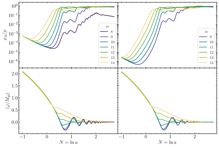
Figure 1: Energy fraction in the gauge fields (top panels) and homogeneous component of the inflaton (bottom panels) for FLRW simulations (left panels) and BSSN simulations (right panels). Note that at early times ($N\lesssim 0$) the gauge field energy densities differ between the two methods only due to the differing choice of cutoffs in initial conditions, as the dominant contribution is from vacuum modes (and unphysical).

The right panel of fig. 1 shows the same quantities when implemented in the BSSN scheme. The inclusion of nonlinear gravity has little to no effect on the qualitative structure of preheating at the level of the background, for the wide range of parameters we have simulated.

Nonetheless, the system exhibits large density contrasts, especially for larger couplings. As a first attempt, we can look for local gravitational effects using a linearized scheme. In conformal Newtonian gauge, where the scalar part of the metric is

$$g^{\rm Newt}_{\mu\nu}=a(\tau)^{2}\operatorname{diag}\left[-\left(1+2\Phi\right),\left(1-2\Phi\right),\left(1-2\Phi\right),\left(1-2\Phi\right)\right],$$ (3.2)

we can solve for the Newtonian potential $\Phi$ with the $00$ component and the (divergence of) the $0i$ components of the Einstein equations. These respectively are

$$\partial_{i}\partial_{i}\Phi-3\mathcal{H}\left(\Phi^{\prime}+\mathcal{H}\Phi\right)=\frac{a^{2}}{2M_{\mathrm{Pl}}^{2}}\delta\rho$$ (3.3)

and

$$\partial_{i}\partial_{i}\left(\Phi^{\prime}+\mathcal{H}\Phi\right)=-\frac{a^{2}}{2M_{\mathrm{Pl}}^{2}}\partial_{i}T_{0i},$$ (3.4)

which we solve using the same method as described in [80]. Figure 2 shows the statistics of the Newtonian potential calculated from our FLRW simulations in fig. 1. In this work, we calculate the Newtonian potential passively—with no feedback onto the evolution of the fields—to show that the Newtonian potential becomes too large, $\Phi>0.25$, to be able to treat gravity to linear order for the specific situations we consider. At this value, $\sqrt{-g^{\rm Newt}}=a^{4}\left(1-4\Phi\right)$ locally changes sign and linearized gravity, in conformal Newtonian gauge, necessarily breaks down.

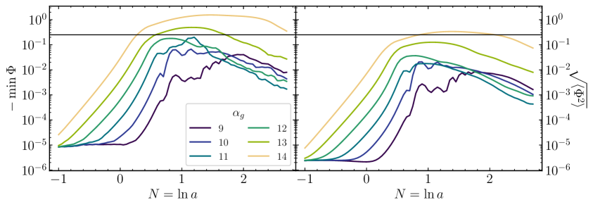
Figure 2: Statistics of the Newtonian potential calculated passively from FLRW simulations. The left panel shows the absolute value of the minimum value of the Newtonian potential on each slice, the right panel shows the square root of the variance of the Newtonian potential across the grid. The solid horizontal lines denote the value $\Phi=0.25$, the point at which linearized gravity breaks down. Curves are not smooth only because these quantities are calculated at relatively infrequent intervals.

3.2 Density contrast and gravitational collapse

While the main features of the preheating story remain unchanged in the presence of nonlinear gravity, we now look to see if the additional nonlinear interactions provided by the gravitational sector affect the modes and scales that participate. Specifically, we search for hints that these interactions may lead to gravitational collapse.

The first place we look is at the power spectrum of density fluctuations. In fig. 3 we plot the dimensionless power spectrum of $\delta\equiv\delta\rho/\bar{\rho}$,

$$\Delta^{2}_{\delta}=\frac{k^{3}}{2\pi^{2}}P_{\delta}(k),$$ (3.5)

where the power spectrum is defined from the two point correlation function,

$$\left<\delta(k)\delta(k^{\prime})\right>=\left(2\pi\right)^{3}\delta^{3}({\bf k}-{\bf k}^{\prime})P_{\delta}(k).$$ (3.6)

When calculating $\Delta^{2}_{\delta}$ we directly Fourier Transform the $\rho$ as calculated in eq. 2.33a on the hypersurfaces of the simulation and ignore spatial dependence of the conformal factor. This measure is often cited as the litmus test for the need to incorporate nonlinear effects (see, for example, Ref. [95]) as well as a useful measure to determine whether primordial black holes are produced. This statistic was first used as a way to diagnose potential primordial black hole formation in Ref. [96] and continues to be used, see, for example, Refs. [29, 97].

Figure 3: Spectra of density fluctuations $\delta=\delta\rho/\bar{\rho}$ in simulations with axial coupling $\alpha$ varying by panel, comparing results from simulations implementing full general relativity via the BSSN scheme (solid blue lines) and FLRW simulations (dashed red). All results are evaluated two $e$-folds after the end of inflation.

Figure 3 shows that, in many cases, dimensionless power spectra are of order $\Delta_{\delta}^{2}(k)\sim 1$ for large $\alpha_{g}$. This is reinforced by the fact that perturbation theory breaks down at these times; more precisely, in cases where $\delta(k)$ approaches unity, the linearized Einstein’s equations are violated as we saw in fig. 2 [88].

As one would expect, the simulations with nonlinear gravity show more numerical effects at high wavenumber; nonetheless, the physical parts of the power spectra are very consistent with the FLRW counterparts. The only exception to this is, perhaps, the very highest values of the self-coupling where there seems to be somewhat higher power at lower scales and somewhat lower power at intermediate scales. We speculate that this is due to the fact that local gravity can lead to some clumping in the nonlinear simulations.

In order for clumps to actually collapse into black holes, overdensities must overcome their own internal pressure. In linear theory, the Jeans scale is used to determine whether the scales of interest can collapse. Modes with wavelength longer than the Jeans length undergo gravitational collapse, while those with shorter wavelength are pressure supported. This scale defines to the (physical) Jeans scale,

$$k_{J}^{\rm phys}=\frac{2\pi}{\lambda_{J}}=2\pi\sqrt{\frac{\rho G}{c_{s}^{2}}}=\sqrt{\frac{3H^{2}}{2\pi c_{s}^{2}}},$$ (3.7)

where $c_{s}^{2}=\delta P/\delta\rho$ is the sound speed. The comoving Jeans scale is $k_{J}=ak_{J}^{\rm phys}$. Since the gauge fields are the main component of the universe, we estimate $c_{s}^{2}=1/3$ to approximate the sound speed for a radiation fluid. At the end of our simulations—where the power spectra in fig. 3 are evaluated—the Jeans scale $k_{J}$ is much smaller than the peak frequency of the dimensionless power spectrum of the density fluctuations. This indicates that the radiation pressure of the gauge fields is playing an important role in the evolution of these structures. To use $\alpha_{g}=13$ and $\alpha_{g}=14$ as examples, we can track the location peak of the dimensionless power spectrum throughout simulation which we can compare to the Jeans scale and the Hubble scale as can be seen in fig. 4. The differences in the evolution of the comoving scales is due to the fact that, for the largest coupling, the gauge field backreaction briefly restarts inflation. Fig. 4 shows us that Jeans-scale modes are excited near the end of inflation; however, these modes are still small. As the density contrast grows, the peak of the power spectrum moves to slightly larger comoving wavenumber, while the comoving Jeans scale shrinks. By the time we reach two $e$-folds after the end of inflation, the peak mode of the power spectrum is approximately a factor of five larger than the Jeans scale.

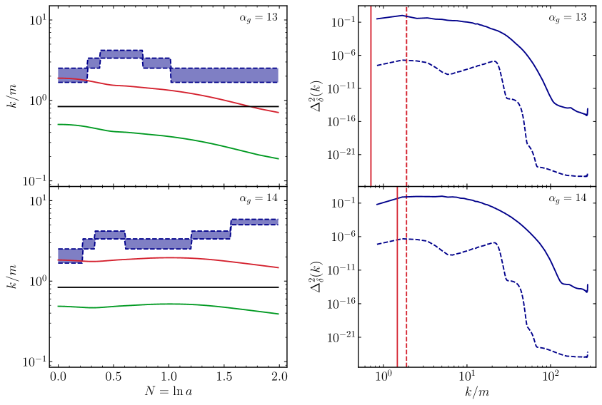
Figure 4: The comoving Jeans scale compared to the dimensionless power spectrum. The left panels show the range of modes in the peak–most power–bin of the dimensionless power spectrum (blue, shaded region) compared to the Jeans scale (red), the Hubble scale (green), and the longest resolvable mode in the box (black). We only calculate the location of the peak of the dimensionless power spectrum and the Jeans length after the end of inflation when the power spectrum raises above its initialized shape and we can approximate the Universe as radiation dominated. The right panels show the dimensionless power spectrum at the end of inflation (blue, dashed lines) and two $e$-folds after the end of inflation (blue, solid lines) with vertical lines showing the Jeans corresponding jeans scale at the end of inflation (red, dashed lines) and two $e$-folds after the end of inflation (red, solid lines). The top panels correspond to $\alpha_{g}=13$ and the bottom panels correspond to $\alpha_{g}=14$.

A number of different tools are used to identify the existence of black holes when studying critical collapse in numerical relativity [83]. In $1+\log$ slicing, where $(\partial_{t}+\beta^{i}\partial_{i})\alpha=-2\alpha K$, the vanishing of the lapse $\alpha$ can sometimes be used as an indicator that black holes have formed [98, 99, 100, 101, 102, 103, 104]. The same is true for our slicing condition, eq. 2.18, where the only difference is the background clock which is constructed to mimic a conformal-time FLRW solution in the homogeneous limit. In the weak gravity limit, we can compute the inhomogeneity of $\alpha$ to measure how much our slices vary from the FLRW limit, with smaller values of $\alpha$ corresponding to deeper gravitational wells. Figure 5 shows 2-dimensional slices of three different simulations evaluated two e-foldings after the end of inflation. In these figures we can see spatial variation in the density contrast—which is often large, $\mathcal{O}(10)$. The lapse, however, does not deviate much more than $\mathcal{O}\left(10^{-1}\right)$.

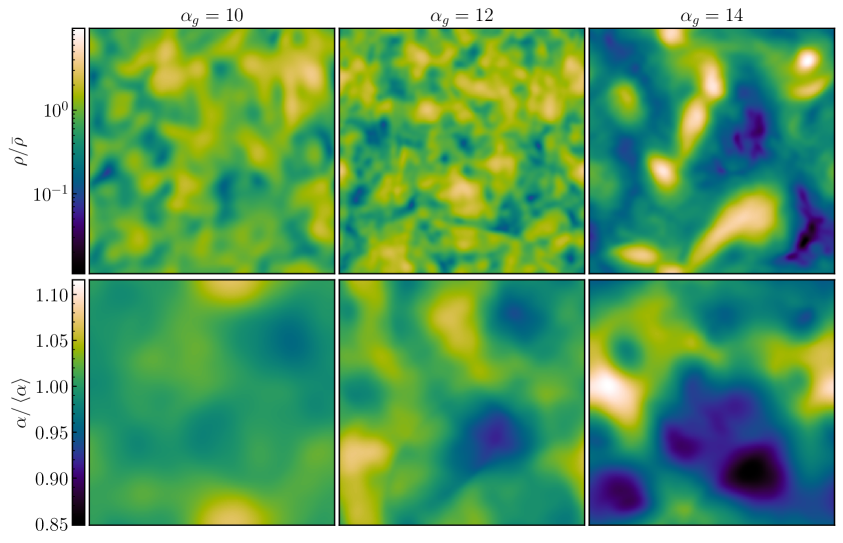
Figure 5: Two-dimensional spatial slices of the density contrast, $\delta$, (top panels) and lapse (normalized to its average over all space; bottom panels), $\alpha/\left<\alpha\right>$. Columns display results for simulations with axial coupling $\alpha_{g}=10,12$, and $14$ from left to right. All results are evaluated two $e$-folds after the end of inflation.

We can extend this to a statistical test by calculating the variance of the density contrast $\delta$ and the lapse $\alpha$ throughout the simulation. As we can see in fig. 6, the variance of the lapse increases with the size of the axial coupling $\alpha_{g}$. However, the deviation from the average is never larger than $\mathcal{O}(0.3)$.

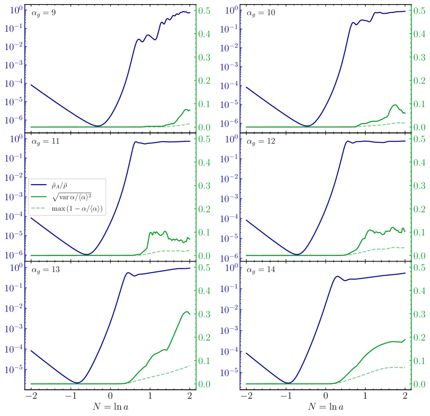
Figure 6: Dynamics of energy transfer and the metric lapse during preheating. Plotted is the fraction of energy in the gauge fields, $\bar{\rho}_{A}/\bar{\rho}$ (solid blue, with scale given by the left of each panel) and the root-mean-squared and maximum deviation of the lapse from its average over space (solid green and transparent, dashed green, respectively, with scale given by the right of each panel). Each panel corresponds to a simulation with axial coupling strength indicated on the plot.

As a final metric, we look to determine whether regions in our simulations have passed thresholds that one might consider sufficient to produce black holes. We begin by examining just one of the more dramatic runs and calculating the compactness [105, 106, 107, 108] generalized to an expanding spacetime [109]

$$C(R)=\frac{G\delta\!M}{R}$$ (3.8)

to calculate whether the overdensities on the final slice indicate that black holes might form. In eq. 3.8 $\delta\!M$ is the instantaneous over-mass enclosed in some (proper) radius, $R$. That is, we subtract off the background density when computing the mass. Note that we use a different definition of compactness than that in Ref. [110], where the authors measure the total integrated $\rho$ within a (not necessarily spherical) region where $\rho/\bar{\rho}>5\%$, although both definitions reduce to a statement of the hoop conjecture [84] about a spherically symmetric overdensity and when $\rho/\bar{\rho}\gg 1$.

To test this, we look at the final slice for the largest coupling we test, $\alpha_{g}=14$, and compute the compactness of the largest over-density in the box. Centering coordinates about the location of maximum $\delta(x)$, we can calculate the enclosed over-mass

$$\delta\!M(R)=\bar{\rho}\int_{0}^{R}\sqrt{\gamma}\left(\delta-1\right)\,r^{2}dr=\bar{\rho}\Delta x^{3}\sum_{i}\sqrt{\gamma_{i}}\left(\delta(x_{i})-1\right).$$ (3.9)

and, following [110], we approximate the radius of this overdensity from $V=4R^{3}/3\pi$,

$$R=\left(\frac{3\pi}{4}\right)^{1/3}\left(\int_{0}^{R}\sqrt{\gamma}r^{2}dr\right)^{1/3}=\left(\frac{3\pi}{4}\right)^{1/3}\left(\Delta x^{3}\sum_{i}\sqrt{\gamma_{i}}\right)^{1/3}.$$ (3.10)

In both eq. 3.9 and eq. 3.10 the final sum is over all points inside a given radius $r$. Figure 7 shows the compactness as a function of distance away from the center—a measure that is maximized around $C\sim 10^{-1}$, yet is still smaller than the critical value of $1/2$. In fig. 7 we also plot the FLRW approximation to the compactness where $\delta\!M_{\rm FLRW}=a^{3}\bar{\rho}\Delta x^{3}\sum_{i}\left(\delta_{i}-1\right)$ and $R_{\rm FLRW}=a\Delta x$ where the scale factor is calculated in the FLRW limit, $a^{2}=\bar{e^{4\phi}}$, see appendix B.

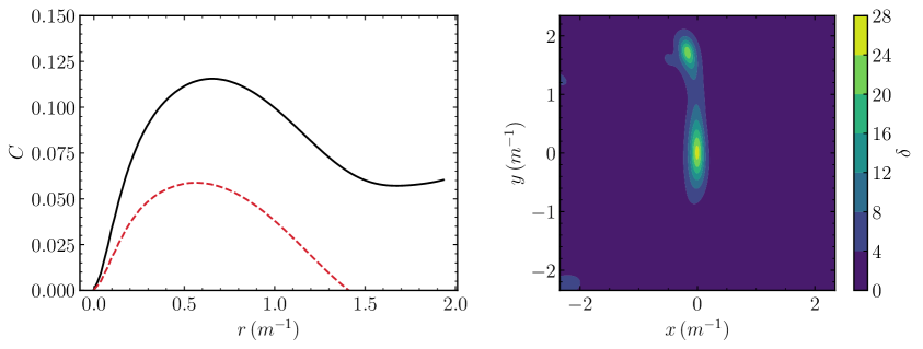
Figure 7: The left panel shows the compactness $C$ as a function of distance from the center of the largest overdensity present in the final slice of the simulation with $\alpha_{g}=14$ (black, solid). We also plot the FLRW approximation to the compactness (red, dashed). The right panel shows the $z={\rm constant}$ slice through the center of the overdensity.

3.3 Gravitational waves

One of the most striking features of gauge preheating is the strength of the production of gravitational radiation. During and after gauge preheating, gravitational wave production can be so strong that the resulting radiation density stored in gravitational waves leads to a shift in the effective number of relativistic species $N_{\rm eff}$ that is large enough to be measured or constrained by current and future CMB experiments [70, 71, 69]. In some models, the shift is large enough that the allowed values of the axial coupling are already constrained by existing CMB measurements. These results were obtained using numerical simulations that ignore the backreaction of these large metric fluctuations. In this section, we explore the robustness of predictions of gravitational wave production during gauge preheating in the regime where gravity is nonlinear.

Gravitational waves are the traceless part of the spatial metric, and are contained in $\bar{\gamma}_{ij}$. In FLRW simulations, the gravitational wave spectrum is computed passively—see, e.g. [23], by calculating the transverse-traceless parts of the matter stress tensor,

$$T_{ij}^{\rm TT}=\left(P_{il}P_{jm}-\frac{1}{2}P_{ij}P_{lm}\right)T_{lm},$$ (3.11)

where $P$ is the projection operator,

$$P_{ij}=\delta_{ij}-\frac{k_{i}k_{j}}{k^{2}}.$$ (3.12)

This sources the transverse-traceless part of the metric via Einstein’s equations

$$\Box h_{ij}=16\pi G\,T^{\rm TT}_{ij}.$$ (3.13)

We can then calculate the power in gravitational waves from the gravitational wave stress-energy tensor [84]

$$T_{\mu\nu}^{\rm GW}=8\pi G\left<h_{ij,\mu}^{\rm TT}{{h^{ij}}_{\nu}}^{\rm TT}\right>$$ (3.14)

where

$$\rho_{\rm gw}^{\rm FLRW}=8\pi G\left|h_{ij,0}^{\rm TT}\right|^{2}.$$ (3.15)

The energy density in gravitational waves at the time of emission is then given by

$$\Omega^{\rm FLRW}_{\rm gw}(k)\equiv\frac{1}{\rho}\frac{\mathrm{d}\rho_{\mathrm{gw}}}{\mathrm{d}\ln k}=\frac{1}{24\pi^{2}L^{3}}\frac{k^{3}}{\mathcal{H}^{2}}\sum_{i,j}\left|h_{ij}^{\prime}(k,\tau))\right|^{2}.$$ (3.16)

Since the BSSN system evolves the entire metric by solving the full nonlinear Einstein equations, the gravitational wave spectrum can be directly extracted by projecting out the transverse-traceless part of the extrinsic curvature, $h_{ij}^{\prime}\approx-2\tilde{A}_{ij}$ [78]. The BSSN analog to eq. (3.16) is then

$$\Omega^{\rm BSSN}_{\rm gw}(k) =\frac{3}{2\pi^{2}L^{3}}\frac{k^{3}}{\left\langle K\right\rangle^{2}}\sum_{i,j}\left|\tilde{A}_{ij}(k,t)\right|^{2},$$ (3.17)

which is analogous to the quantities used in Refs. [79, 111].

The spectral energy density of gravitational waves today can be calculated using the standard transfer functions [20, 21], assuming that the signal is evaluated during a radiation-dominated period and remains radiation dominated until matter-radiation equality. The spectral energy density today is given by

$$\Omega_{\mathrm{GW},0}h^{2} =\Omega_{\mathrm{rad},0}h^{2}\left(\frac{g_{\star S}(a_{0})}{g_{\star S}(a_{\mathrm{r}})}\right)^{1/3}\Omega_{\mathrm{GW}}(a),$$ (3.18)

and the frequency by

$$f =\frac{k/2\pi a}{\rho(a)^{1/4}}\rho_{\mathrm{r}}(a_{0})^{1/4}\left(\frac{g_{\star}(a_{\mathrm{r}})}{g_{\star}(a_{0})}\right)^{1/4}\left(\frac{g_{\star S}(a_{\mathrm{r}})}{g_{\star S}(a_{0})}\right)^{-1/3}$$ (3.19)

$$=3.2\times 10^{10}\,\mathrm{Hz}\frac{k/a}{\sqrt{H(a)M_{\mathrm{Pl}}}}\left(\frac{g_{\star}(a_{\mathrm{r}})/g_{\star}(a_{0})}{100}\right)^{-1/12}.$$ (3.20)

In the preceding expressions $g_{\star}$ is the number of ultra-relativistic degrees of freedom evaluated at reheating ($a_{r}$) or today ($a_{0}$). For simplicity, we take $g_{\star}(a_{\mathrm{r}})/g_{\star}(a_{0})\approx 100$.

In fig. 8 we show the gravitational wave spectra from simulations of gauge preheating in both full nonlinear gravity, as well as in rigid FLRW spacetime. Despite the presence of strong nonlinearities, we observe remarkably consistent outputs across the range of couplings we considered. These results suggest that neglecting nonlinear gravity has at most an $\mathcal{O}(1)$ effect on the resulting gravitational wave spectrum, even in regions where the metric is highly nonlinear.

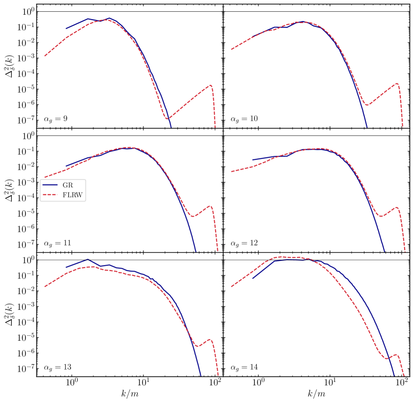
Figure 8: Present-day gravitational wave spectra in simulations with axial coupling $\alpha_{g}$ varying by panel, comparing results from simulations implementing full general relativity via the BSSN scheme (solid blue lines) and FLRW simulations (dashed red). All results are evaluated two $e$-folds after the end of inflation.

4 Conclusions

In this paper we have extended studies of gauge preheating after pseudoscalar-driven inflation to include the effects of nonlinear gravitation. To facilitate this study, we implemented numerical relativity using the BSSN formalism in our simulation software.

The evolution of the energy density and fields was nearly indistinguishable from simulations done in a FLRW spacetime. Including the effects of nonlinear gravity made no qualitative difference in the value or evolution of the averaged background quantities, such as the expansion rate, the average value of the scalar field, or the energy densities of the scalar and gauge fields.

In our FLRW simulations we observed the emergence of regions with very large fractional overdensities $\delta\rho/\rho$, which routinely exceeded unity. The existence of these regions leads to the failure of linearized gravity, requiring software that properly treats evolution of the metric into the nonlinear regime. In our BSSN simulations, we observe power being shifted from large to small scales due to the gravitational interactions.

In our highest-coupling BSSN runs, we found regions with fractional overdensities as large as $\delta\rho/\rho\sim 30$. However, despite the development of these large density contrasts we found no evidence for the formation of black holes such as the presence of horizons or the vanishing of the lapse function. Closer examination of these simulations revealed that the scales where the density power spectrum peaks are within the Jeans length. This suggests that pressure of the radiation plays an important role in the evolution and stability or instability of these very overdense regions. We also computed the compactness of these regions, and found that it peaks at values $C\sim 10^{-1}$, which is somewhat below the level required to make a black hole of $C\sim 0.5$.

We also studied the resulting spectrum of gravitational waves in these scenarios. A key result of our earlier work was the prediction of a very large gravitational wave signal at the strongest couplings. Our simulations in full nonlinear gravity revealed the robustness of our original FLRW simulations of gravitational wave production.

Looking further ahead, our BSSN simulations of gauge preheating end sooner than would be ideal, owing to the large increase in the volume of the box over the course of four $e$-foldings of expansion and the movement of power to large wave number after this time. We plan to investigate the dynamics of the large overdense regions to study their fate. In particular, it would be interesting to investigate whether the large overdensities subsequently undergo gravitational collapse, or whether they simply decay. Our simulations have so far focused on the large density fluctuations that are generated on sub-horizon scales during reheating. These are necessarily inside the Jeans length at production. It would be interesting to study the horizon reentry of large curvature perturbations that are produced near the end of inflation in these models to see if their collapse to black holes can be verified in full general relativity.

Appendix A BSSN decomposition

In this appendix we present the details of our decomposition of the gauge fields in the BSSN formalism. We begin by detailing the $3+1$ decomposition of the metric and the foliation of the spacetime in section A.1, before detailing the equations of motion for the scalar and gauge fields in section A.2, and the derivation of the stress-energy tensor and sources for the evolution of the BSSN system in section A.3.

A.1 3 + 1 decomposition

The line element in $3+1$ form is

$$\mathrm{d}s^{2} =-\alpha^{2}\mathrm{d}t^{2}+\gamma_{ij}\left(\mathrm{d}x^{i}+\beta^{i}\mathrm{d}t\right)\left(\mathrm{d}x^{j}+\beta^{j}\mathrm{d}t\right),$$ (A.1)

where the lapse $\alpha$ and shift $\beta^{i}$ parameterize gauge degrees of freedom, while the spatial metric $\gamma_{ij}$ and $\gamma^{ij}$ are used to lower and raise indices of spatial tensors. The lapse and shift define the normal vector to hypersurfaces,

$$n^{\mu}=\frac{1}{\alpha}\left(1,-\beta^{i}\right).$$ (A.2)

From the normalization condition of the normal vector, $n_{\mu}n^{\mu}=-1$, we can calculate its inverse,

$$n_{\mu} =(-\alpha,0,0,0).$$ (A.3)

The projector onto spatial hypersurfaces is

$$\gamma^{\mu}_{\hphantom{\mu}\nu}=\delta^{\mu}_{\hphantom{\mu}\nu}+n^{\mu}n_{\nu}.$$ (A.4)

The 3-dimensional covariant derivative is

$$D_{\mu}f\equiv\gamma_{\mu}^{\hphantom{\mu}\nu}\nabla_{\nu}f,$$ (A.5)

which is expressed via the 3-dimensional connection coefficients,

$$\Gamma^{i}_{\hphantom{i}jk}=\frac{1}{2}\gamma^{il}\left(\partial_{k}\gamma_{lj}+\partial_{j}\gamma_{lk}-\partial_{l}\gamma_{jk}\right).$$ (A.6)

The extrinsic curvature tensor is

$$K_{\mu\nu} =-\gamma_{\mu}^{\hphantom{\mu}\alpha}\gamma_{\nu}^{\hphantom{\nu}\beta}\nabla_{\alpha}n_{\beta},$$ (A.7)

and its trace is

$$K\equiv g^{\mu\nu}K_{\mu\nu} =-\nabla^{\alpha}n_{\alpha}.$$ (A.8)

A.2 Equations of motion

For completeness, we generalize the action eq. 2.1 to include a kinetic coupling $W(\varphi)$,

$$S =\int\mathrm{d}^{4}x\,\sqrt{-g}\left[\frac{M_{\mathrm{Pl}}^{2}}{2}R-\frac{1}{2}\nabla_{\mu}\varphi\nabla^{\mu}\varphi-V(\varphi)-\frac{W(\phi)}{4}F_{\mu\nu}F^{\mu\nu}-\frac{X(\varphi)}{4}F_{\mu\nu}\tilde{F}^{\mu\nu}\right].$$ (A.9)

A.2.1 Scalar fields

Starting with the action eq. A.9, the Euler-Lagrange equation for the scalar field is

$$-\nabla_{\mu}\nabla^{\mu}\varphi=\frac{\partial{\mathcal{L}}}{\partial{\varphi}} =-\frac{\mathrm{d}{V}}{\mathrm{d}{\varphi}}-\frac{1}{4}\frac{\mathrm{d}{W}}{\mathrm{d}{\varphi}}F_{\mu\nu}F^{\mu\nu}-\frac{1}{4}\frac{\mathrm{d}{X}}{\mathrm{d}{\varphi}}F_{\mu\nu}\tilde{F}^{\mu\nu}.$$ (A.10)

To rewrite this in the $3+1$ form, we must first decompose $\nabla_{\mu}\varphi$ into its parts normal to ($\Pi$) and lying in ($D_{\mu}\varphi$) spatial hypersurfaces,

$$\nabla_{\nu}\varphi =D_{\nu}\varphi-n_{\nu}\Pi.$$ (A.11)

This defines the scalar’s conjugate momentum,

$$\Pi \equiv n^{\mu}\nabla_{\mu}\varphi=\frac{1}{\alpha}\left(\nabla_{0}\varphi-\beta^{k}\nabla_{k}\varphi\right).$$ (A.12)

A similar expansion of the covariant d’Alembertian yields

$$\nabla^{\mu}\nabla_{\mu}\varphi =\frac{1}{\alpha}\gamma^{ij}D_{i}\alpha D_{j}\varphi+\gamma^{ij}\left(\partial_{i}D_{j}\varphi-\Gamma^{k}_{\hphantom{k}ij}D_{k}\varphi\right)+K\Pi-\frac{1}{\alpha}\left(\partial_{t}\Pi-\beta^{k}D_{k}\Pi\right).$$ (A.13)

Rearranging eq. A.10 into an explicit evolution equation for $\Pi$,

$$\partial_{t}\Pi =\beta^{k}D_{k}\Pi+\gamma^{ij}\left(\alpha\partial_{i}D_{j}\varphi+D_{i}\alpha D_{j}\varphi\right)+\alpha\left(K\Pi-\gamma^{ij}\Gamma^{k}_{\hphantom{k}ij}D_{k}\varphi-\frac{\partial{\mathcal{L}}}{\partial{\varphi}}\right),$$ (A.14)

while solving eq. A.12 for $\partial_{t}\varphi$ yields

$$\partial_{t}\varphi=\beta^{k}D_{k}\varphi+\alpha\Pi.$$ (A.15)

To increase numerical stability, we promote the spatial derivatives of the scalar field to dynamical degrees of freedom themselves,

$$\psi_{i}\equiv D_{i}\varphi.$$ (A.16)

These evolve according to the gradient of eq. A.15,

$$\partial_{t}\psi_{i} =\beta^{k}\partial_{k}\psi_{i}+\psi_{k}\partial_{i}\beta^{k}+\alpha D_{i}\Pi+\Pi D_{i}\alpha.$$ (A.17)

Using this variable, eq. A.14 becomes

$$\partial_{t}\Pi =\beta^{k}D_{k}\Pi+\gamma^{ij}\left(\alpha\partial_{i}\psi_{j}+D_{i}\alpha\psi_{j}\right)+\alpha\left(K\Pi-\gamma^{ij}\Gamma^{k}_{\hphantom{k}ij}\psi_{k}-\frac{\partial{\mathcal{L}}}{\partial{\varphi}}\right),$$ (A.18)

which gives us the full system, eq. 2.28.

A.2.2 Gauge fields

Again, starting with the model eq. A.9, the Euler-Lagrange equations for the gauge field are

$$0 =W(\varphi)\nabla^{\alpha}F_{\alpha\beta}+\partial^{\alpha}W(\varphi)F_{\alpha\beta}+\partial^{\alpha}X(\varphi)\tilde{F}_{\alpha\beta},$$ (A.19)

which may be rearranged into canonical form as

$$\nabla_{\mu}F^{\mu\nu} =-\frac{1}{W(\varphi)}\left(\partial_{\mu}W(\varphi)F^{\mu\nu}+\partial_{\mu}X(\varphi)\tilde{F}^{\mu\nu}\right)\equiv-J^{\nu}.$$ (A.20)

In the last line we define the “source vector” $J^{\nu}$ to encode the coupling to the scalar.

To recast these into the BSSN formalism, we begin by splitting the vector potential $A_{\mu}$ into its components along and orthogonal to spatial hypersurfaces,

$$A_{\mu}\equiv\mathcal{A}_{\mu}+n_{\mu}\mathcal{A},$$ (A.21)

where $\mathcal{A}_{\mu}=\gamma_{\mu}^{\hphantom{\mu}\nu}A_{\nu}$ and $\mathcal{A}=-n^{\nu}A_{\nu}$. The electric and magnetic fields are

$$E^{\mu} =\gamma^{\mu}_{\hphantom{\mu}\nu}n_{\alpha}F^{\nu\alpha}$$ (A.22)

$$B^{\mu} =-\gamma^{\mu}_{\hphantom{\mu}\nu}n_{\alpha}\tilde{F}^{\nu\alpha}$$ (A.23)

$$=\frac{1}{2}\epsilon^{\mu\alpha\rho\gamma}n_{\alpha}F_{\gamma\rho}.$$ (A.24)

In terms of these variables, the field tensor is

$$F_{\mu\nu} =n_{\mu}E_{\nu}-n_{\nu}E_{\mu}+D_{\mu}\mathcal{A}_{\nu}-D_{\nu}\mathcal{A}_{\mu},$$ (A.25)

or equivalently

$$F^{\mu\nu} =n^{\mu}E^{\nu}-n^{\nu}E^{\mu}+n_{\sigma}\epsilon^{\sigma\mu\nu\rho}B_{\rho}.$$ (A.26)

We also decompose the source vector analogously to the gauge field, eq. A.21:

$$J^{\mu} \equiv\mathcal{J}^{\mu}+n^{\mu}\mathcal{J}.$$ (A.27)

We can extend the gauge field system to include a constraint damping field $Z$ as [90, 91, 92, 93]

$$\nabla_{\mu}F^{\mu\nu}+J^{\nu}-\frac{1}{W(\varphi)}\left(\nabla^{\nu}Z-\kappa n^{\nu}Z\right)=0$$ (A.28a)

and

$$\nabla^{\mu}A_{\mu}+Z=0.$$ (A.28b)

We can now set Lorenz gauge, $\nabla^{\mu}A_{\mu}+Z=0$, to obtain the evolution equation for $\mathcal{A}$. Expanding the covariant divergence in terms of the $3+1$ decomposition and rearranging gives

$$\partial_{t}\mathcal{A} =\beta^{k}D_{k}\mathcal{A}+\alpha\left(K\mathcal{A}-D^{i}\mathcal{A}_{i}-Z\right)-\mathcal{A}_{i}D^{i}\alpha.$$ (A.29)

The dynamics of $\mathcal{A}_{i}$ follow from the definition of $E_{i}$:

$$\partial_{t}\mathcal{A}_{i} =\beta^{k}\partial_{k}\mathcal{A}_{i}+\mathcal{A}_{k}\partial_{i}\beta^{k}-\mathcal{A}D_{i}\alpha-\alpha\left(E_{i}+D_{i}\mathcal{A}\right).$$ (A.30)

The electric field’s own evolution equation comes from the projection of Maxwell’s equation eq. A.28a onto spatial hypersurfaces,

$$\partial_{t}E^{i} =\beta^{k}\partial_{k}E^{i}-E^{k}\partial_{k}\beta^{i}+\alpha\left(KE^{i}-\mathcal{J}^{i}+\frac{1}{W(\varphi)}D^{i}Z\right)+\epsilon^{ijk}D_{j}\left(\alpha B_{k}\right).$$ (A.31)

Note that the latter term may be rewritten as

$$\epsilon^{ijk}D_{j}\left(\alpha B_{k}\right) =D_{j}\left(\alpha D_{i}\mathcal{A}_{j}-D_{j}\mathcal{A}_{i}\right).$$ (A.32)

The spatial component of the source vector evaluates to

$$\mathcal{J}^{i} =\frac{1}{W(\varphi)}\left(\frac{\mathrm{d}{W}}{\mathrm{d}{\varphi}}\left[\Pi E^{i}-\epsilon^{ijk}D_{j}\varphi B_{k}\right]+\frac{\mathrm{d}{X}}{\mathrm{d}{\varphi}}\left[-\Pi B^{i}-\epsilon^{ijk}D_{j}\varphi E_{k}\right]\right).$$ (A.33)

Finally, when the constraint damping field $Z=0$, the component of eq. A.19 normal to spatial hypersurfaces yields Gauss’s law,

$$D_{i}E^{i} =\mathcal{J},$$ (A.34)

where

$$\mathcal{J} =-\frac{1}{W(\varphi)}\left(\frac{\mathrm{d}{W}}{\mathrm{d}{\varphi}}E^{i}D_{i}\varphi-\frac{\mathrm{d}{X}}{\mathrm{d}{\varphi}}B^{i}D_{i}\varphi\right).$$ (A.35)

When including the constraint damping field, this equation instead specifies the dynamics of $Z$. Namely, eq. A.34 reads

$$D_{\mu}E^{\mu}-\mathcal{J}-\frac{1}{W(\varphi)}\left(\frac{1}{\alpha}\left[\partial_{t}Z-\beta^{k}D_{k}Z\right]+\kappa Z\right)=0,$$ (A.36)

yielding the evolution equation

$$\partial_{t}Z =\beta^{k}D_{k}Z-\alpha\kappa Z+\alpha W(\varphi)\left(D_{i}E^{i}-\mathcal{J}\right).$$ (A.37)

A.3 Stress-energy tensor

The $3+1$ Einstein equations are written in terms of the following projections of the stress-energy tensor (see, e.g. [83]):

$$\rho \equiv n^{\alpha}n^{\beta}T_{\alpha\beta}$$ (A.38a)

$$S_{\mu} \equiv-\gamma_{\mu}^{\hphantom{\mu}\alpha}n^{\beta}T_{\alpha\beta}$$ (A.38b)

$$S_{\mu\nu} \equiv\gamma_{\mu}^{\hphantom{\mu}\alpha}\gamma_{\nu}^{\hphantom{\nu}\beta}T_{\alpha\beta}$$ (A.38c)

$$S \equiv\gamma^{\alpha\beta}S_{\alpha\beta}.$$ (A.38d)

By construction, $S_{\mu}$ and $S_{\mu\nu}$ are spatial.

We write the total stress tensor as a sum of contributions from the scalar and gauge field, $T_{\mu\nu}\equiv T_{\mu\nu}^{\varphi}+T_{\mu\nu}^{A}$. The scalar-field stress-energy tensor,

$$T_{\mu\nu}^{\varphi} =\nabla_{\mu}\varphi\nabla_{\nu}\varphi+g_{\mu\nu}\left(-\frac{1}{2}\partial_{\alpha}\varphi\partial^{\alpha}\varphi-V(\varphi)\right),$$ (A.39)

decomposes as

$$\rho^{\varphi} =\frac{1}{2}\Pi^{2}+\frac{1}{2}D_{i}\varphi D^{i}\varphi+V(\varphi)$$ (A.40a)

$$S_{\mu}^{\varphi} =-\Pi D_{\mu}\varphi$$ (A.40b)

$$S_{\mu\nu}^{\varphi} =D_{\mu}\varphi D_{\nu}\varphi-\gamma_{\mu\nu}\left(-\frac{1}{2}\Pi^{2}+\frac{1}{2}D_{i}\varphi D^{i}\varphi+V(\varphi)\right)$$ (A.40c)

$$S^{\varphi} =\frac{3}{2}\Pi^{2}-\frac{1}{2}D_{i}\varphi D^{i}\varphi-3V(\varphi).$$ (A.40d)

The stress-energy tensor for the gauge field is

$$T_{\mu\nu}^{A} =g^{\alpha\beta}F_{\mu\alpha}F_{\nu\beta}-g_{\mu\nu}\frac{1}{4}F_{\alpha\beta}F^{\alpha\beta},$$ (A.41)

and its $3+1$ components are

$$\rho^{A} =\frac{W(\varphi)}{2}\left(E_{\alpha}E^{\alpha}+B_{\alpha}B^{\alpha}\right)$$ (A.42a)

$$S_{\mu}^{A} =W(\varphi)\epsilon_{\mu\alpha\rho}E^{\alpha}B^{\rho}$$ (A.42b)

$$S_{\mu\nu}^{A} =W(\varphi)\left(-E_{\mu}E_{\nu}-B_{\mu}B_{\nu}+\frac{1}{2}\gamma_{\mu\nu}\left(E_{\alpha}E^{\alpha}+B_{\alpha}B^{\alpha}\right)\right)$$ (A.42c)

$$S^{A} =\frac{W(\varphi)}{2}\left(E_{\alpha}E^{\alpha}+B_{\alpha}B^{\alpha}\right).$$ (A.42d)

Appendix B Perturbation theory

In this appendix, we detail perturbation theory in the BSSN formalism and describe how we set initial conditions in the BSSN code.

B.1 Metric perturbations

We define the perturbed metric

$$g_{\mu\nu}\equiv a(\tau)^{2}\left(\eta_{\mu\nu}+h_{\mu\nu}\right)$$ (B.1)

where $h_{\mu\nu}$ is a small perturbation with scalar-vector-tensor decomposition

$$h_{00} =-E$$ (B.2a)

$$h_{i0} =\partial_{i}F+G_{i}$$ (B.2b)

$$h_{ij} =A\delta_{ij}+\partial_{i}\partial_{j}B+\partial_{i}C_{j}+\partial_{j}C_{i}+D_{ij}.$$ (B.2c)

Here $C_{i}$ and $G_{i}$ are transverse vectors—namely, $\partial_{i}C_{i}=0$ and $\partial_{i}G_{i}=0$—and $D_{ij}$ is transverse ($\partial_{i}D_{ik}=0$) and traceless ($D_{ii}=0$).

We expand the BSSN variables to linear order about a homogeneous and isotropic background spacetime as

$$\alpha =\alpha_{0}+\delta\alpha$$ (B.3a)

$$\beta^{i} =0+\delta\beta^{i}$$ (B.3b)

$$\phi =\phi_{0}+\delta\phi$$ (B.3c)

$$\bar{\gamma}_{ij} =\delta_{ij}+\delta\gamma_{ij}$$ (B.3d)

$$K =K_{0}+\delta K$$ (B.3e)

$$\tilde{A}_{ij} =0+a_{ij}.$$ (B.3f)

Expanding the BSSN metric in these variables, we identify

$$e^{4\phi_{0}}=\alpha_{0}(\tau)^{2}$$ (B.4)

or

$$\phi_{0}=\frac{\ln\alpha_{0}}{2},$$ (B.5)

and

$$\frac{\delta\alpha}{\alpha_{0}} =E$$ (B.6)

$$\beta_{i} =a(\tau)^{2}\left(\partial_{i}F+G_{i}\right)$$ (B.7)

$$4\delta\phi =A$$ (B.8)

$$\delta\gamma_{ij} =\partial_{i}\partial_{j}B+\partial_{i}C_{j}+\partial_{j}C_{i}+D_{ij}.$$ (B.9)

We can linearize the equation of motion for $\bar{\gamma}_{ij}$ to obtain

$$\partial_{t}\bar{\gamma}_{mn} =-2\alpha_{0}a_{mn}+\delta_{mo}\partial_{n}\delta\beta^{o}+\delta_{on}\partial_{m}\delta\beta^{o}-\frac{2}{3}\delta_{mn}\partial_{o}\delta\beta^{o},$$ (B.10)

which allows us to identify gravitational waves (in the linearized theory) as

$$\partial_{t}D_{mn} =-2\alpha_{0}a_{mn}^{\mathrm{TT}}$$ (B.11)

The trace of the extrinsic curvature, $K$, expands to

$$K\equiv-\frac{6}{\alpha}\partial_{t}\phi =-\frac{6}{\alpha_{0}}\left(1-\frac{\delta\alpha}{\alpha_{0}}\right)\left(\partial_{t}\phi_{0}+\partial_{t}\delta\phi\right)$$ (B.12)

$$=-\frac{6}{\alpha_{0}}\left(\partial_{t}\phi_{0}+\partial_{t}\delta\phi-\partial_{t}\phi_{0}\frac{\delta\alpha}{\alpha_{0}}\right).$$ (B.13)

The background component is

$$K_{0} =-\frac{6}{\alpha_{0}}\partial_{t}\phi_{0},$$ (B.14)

which, using eq. B.4, corresponds to the (cosmic-time) Hubble parameter $H=\mathcal{H}/a$ via

$$K_{0}=-\frac{6}{a}\frac{\partial_{t}\ln a}{2}=-3\frac{\partial_{t}a}{a^{2}}=-3H,$$ (B.15)

remembering that $\partial_{t}$ in the BSSN formalism corresponds to conformal time for our particular gauge choices.

B.2 Initial conditions

The linearized tensor parts of $a_{ij}$ and $\delta\gamma_{ij}$, eq. B.3, comprise genuine, propagating degrees of freedom, so their initial condition is specified independent of constraints. We therefore choose $D_{ij}=0$ and $D_{ij}^{\prime}=0$ from eq. B.2 initially. The remaining degrees of freedom are either gauge choices or set by constraints. We take $\beta^{i}=\delta\beta^{i}=0$ as an initial condition. Correspondingly, we set $F=0$ and $G_{i}=0$ from eq. B.2, amounting to the fixing of two vector and one scalar gauge modes. The initial conditions are simplest to solve for when taking $B=0$ as the final gauge choice.

We define the short-hand

$$y(\mathbf{x}) =\frac{1}{\nabla^{2}}f(\mathbf{x})\equiv\int\frac{\mathrm{d}^{3}k}{(2\pi)^{3}}\frac{e^{i\mathbf{k}\cdot\mathbf{x}}}{-k^{2}}\int\mathrm{d}^{3}y\,e^{-i\mathbf{k}\cdot\mathbf{y}}f(\mathbf{y})$$ (B.16)

to denote the solution to Poisson’s equation, $\nabla^{2}y(\mathbf{x})=f(\mathbf{x})$. The constraint on the vectors may be solved straightforwardly via

$$\frac{1}{2\alpha_{0}}\partial_{t}C_{m} =-\frac{1}{M_{\mathrm{Pl}}^{2}}\frac{1}{\nabla^{2}}\mathcal{S}_{m}.$$ (B.17)

This sets the vector contribution $a_{mn}$ as $-\partial_{(n}\partial_{t}C_{m)}/2\alpha_{0}$. For the scalar degrees of freedom, with $B=0$ one may directly solve the scalar part of the momentum constraint as

$$\delta K =-\frac{3}{2M_{\mathrm{Pl}}^{2}}\frac{1}{\nabla^{2}}\partial_{m}S_{m}.$$ (B.18)

With this solution, we can compute

$$\frac{\delta\psi}{\psi_{0}} =\frac{\psi_{0}^{4}}{\nabla^{2}}\left(\frac{1}{6}K_{0}\delta K-\frac{1}{4M_{\mathrm{Pl}}^{2}}\delta\rho\right).$$ (B.19)

Finally, Gauss’s law expands to

$$\mathcal{J}=\partial_{i}E^{i} =\partial_{i}\partial_{t}\mathcal{A}^{i}-\partial_{i}\partial^{i}\mathcal{A},$$ (B.20)

and, since we take $\partial_{i}\partial_{t}\mathcal{A}^{i}=0$ initially, we satisfy this constraint by setting

$$\mathcal{A} =-\frac{1}{\nabla^{2}}\mathcal{J}.$$ (B.21)

Appendix C Robustness checks

For the six BSSN simulations presented here, we calculate the violation of the Hamiltonian and momentum constraints, eqs. 2.16 and 2.17, and of Gauss’ Law, eq. 2.32, to ensure that we stay on the solution surface of the problem. In fig. 9 we plot these constraints vs $N\equiv\ln a$ to show that they are bounded throughout the simulation.

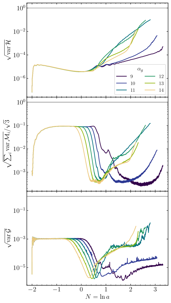
Figure 9: Statistics of violations of the Hamiltonian [$\mathcal{H}$, eq. 2.16], momentum [$\mathcal{M}_{i}$, eq. 2.17], and Gauss [$\mathcal{G}$, eq. 2.32] constraints. Note that we in the main text we only present results up to $N=2$.

For the results presented in this work, we take a conservative cutoff of $N=2$ as a final time. This allows us to consider all of the BSSN simulations in regime where the constraints are small.

For FLRW simulations, the first Friedmann equation, $H^{2}=\rho/3M_{\mathrm{Pl}}^{2}$, serves as a constraint that measures the analog of energy conservation in flat space; the simulations satisfy it to one part in $10^{4}$ or better. The gauge constraints are likewise satisfied to one part in $10^{3}\div 10^{2}$ (see Refs. [35, 36, 69, 70] for further discussion of the robustness of these methods). The FLRW results are all consistent with those of lower-resolution simulations presented in Refs. [69, 70, 71].

References

- [1] A. H. Guth, The Inflationary Universe: A Possible Solution to the Horizon and Flatness Problems, Phys. Rev. D 23 (1981) 347–356.
- [2] A. D. Linde, A New Inflationary Universe Scenario: A Possible Solution of the Horizon, Flatness, Homogeneity, Isotropy and Primordial Monopole Problems, Phys. Lett. B 108 (1982) 389–393.
- [3] A. Albrecht and P. J. Steinhardt, Cosmology for Grand Unified Theories with Radiatively Induced Symmetry Breaking, Phys. Rev. Lett. 48 (1982) 1220–1223.
- [4] A. D. Linde, Chaotic Inflation, Phys. Lett. B 129 (1983) 177–181.
- [5] L. F. Abbott, E. Farhi and M. B. Wise, Particle Production in the New Inflationary Cosmology, Phys. Lett. B 117 (1982) 29.
- [6] A. Albrecht, P. J. Steinhardt, M. S. Turner and F. Wilczek, Reheating an Inflationary Universe, Phys. Rev. Lett. 48 (1982) 1437.
- [7] J. H. Traschen and R. H. Brandenberger, Particle Production During Out-of-equilibrium Phase Transitions, Phys. Rev. D 42 (1990) 2491–2504.
- [8] Y. Shtanov, J. H. Traschen and R. H. Brandenberger, Universe reheating after inflation, Phys. Rev. D 51 (1995) 5438–5455, [hep-ph/9407247].
- [9] L. Kofman, A. D. Linde and A. A. Starobinsky, Reheating after inflation, Phys. Rev. Lett. 73 (1994) 3195–3198, [hep-th/9405187].
- [10] L. Kofman, A. D. Linde and A. A. Starobinsky, Towards the theory of reheating after inflation, Phys. Rev. D 56 (1997) 3258–3295, [hep-ph/9704452].
- [11] P. B. Greene, L. Kofman, A. D. Linde and A. A. Starobinsky, Structure of resonance in preheating after inflation, Phys. Rev. D 56 (1997) 6175–6192, [hep-ph/9705347].
- [12] D. I. Kaiser, Preheating in an expanding universe: Analytic results for the massless case, Phys. Rev. D 56 (1997) 706–716, [hep-ph/9702244].
- [13] M. Parry and R. Easther, Preheating and the Einstein field equations, Phys. Rev. D 59 (1999) 061301, [hep-ph/9809574].
- [14] B. A. Bassett, D. I. Kaiser and R. Maartens, General relativistic preheating after inflation, Phys. Lett. B 455 (1999) 84–89, [hep-ph/9808404].
- [15] R. Easther and M. Parry, Gravity, parametric resonance and chaotic inflation, Phys. Rev. D 62 (2000) 103503, [hep-ph/9910441].
- [16] B. A. Bassett, F. Tamburini, D. I. Kaiser and R. Maartens, Metric preheating and limitations of linearized gravity. 2., Nucl. Phys. B 561 (1999) 188–240, [hep-ph/9901319].
- [17] G. N. Felder and L. Kofman, Nonlinear inflaton fragmentation after preheating, Phys. Rev. D 75 (2007) 043518, [hep-ph/0606256].
- [18] M. A. Amin, M. P. Hertzberg, D. I. Kaiser and J. Karouby, Nonperturbative Dynamics Of Reheating After Inflation: A Review, Int. J. Mod. Phys. D 24 (2014) 1530003, [1410.3808].
- [19] S. Y. Khlebnikov and I. I. Tkachev, Relic gravitational waves produced after preheating, Phys. Rev. D 56 (1997) 653–660, [hep-ph/9701423].
- [20] R. Easther and E. A. Lim, Stochastic gravitational wave production after inflation, JCAP 04 (2006) 010, [astro-ph/0601617].
- [21] R. Easther, J. T. Giblin, Jr. and E. A. Lim, Gravitational Wave Production At The End Of Inflation, Phys. Rev. Lett. 99 (2007) 221301, [astro-ph/0612294].
- [22] J. Garcia-Bellido and D. G. Figueroa, A stochastic background of gravitational waves from hybrid preheating, Phys. Rev. Lett. 98 (2007) 061302, [astro-ph/0701014].
- [23] R. Easther, J. T. Giblin and E. A. Lim, Gravitational Waves From the End of Inflation: Computational Strategies, Phys. Rev. D 77 (2008) 103519, [0712.2991].
- [24] J. F. Dufaux, A. Bergman, G. N. Felder, L. Kofman and J.-P. Uzan, Theory and Numerics of Gravitational Waves from Preheating after Inflation, Phys. Rev. D 76 (2007) 123517, [0707.0875].
- [25] J.-F. Dufaux, G. Felder, L. Kofman and O. Navros, Gravity Waves from Tachyonic Preheating after Hybrid Inflation, JCAP 03 (2009) 001, [0812.2917].
- [26] J.-F. Dufaux, D. G. Figueroa and J. Garcia-Bellido, Gravitational Waves from Abelian Gauge Fields and Cosmic Strings at Preheating, Phys. Rev. D 82 (2010) 083518, [1006.0217].
- [27] A. M. Green and K. A. Malik, Primordial black hole production due to preheating, Phys. Rev. D 64 (2001) 021301, [hep-ph/0008113].
- [28] K. Jedamzik, M. Lemoine and J. Martin, Collapse of Small-Scale Density Perturbations during Preheating in Single Field Inflation, JCAP 09 (2010) 034, [1002.3039].
- [29] J. Martin, T. Papanikolaou and V. Vennin, Primordial black holes from the preheating instability in single-field inflation, JCAP 01 (2020) 024, [1907.04236].
- [30] P. Auclair and V. Vennin, Primordial black holes from metric preheating: mass fraction in the excursion-set approach, JCAP 02 (2021) 038, [2011.05633].
- [31] T. Bringmann, P. Scott and Y. Akrami, Improved constraints on the primordial power spectrum at small scales from ultracompact minihalos, Phys. Rev. D 85 (2012) 125027, [1110.2484].
- [32] G. Aslanyan, L. C. Price, J. Adams, T. Bringmann, H. A. Clark, R. Easther et al., Ultracompact minihalos as probes of inflationary cosmology, Phys. Rev. Lett. 117 (2016) 141102, [1512.04597].
- [33] C. Armendariz-Picon, M. Trodden and E. J. West, Preheating in derivatively-coupled inflation models, JCAP 04 (2008) 036, [0707.2177].
- [34] J. T. Deskins, J. T. Giblin and R. R. Caldwell, Gauge Field Preheating at the End of Inflation, Phys. Rev. D 88 (2013) 063530, [1305.7226].
- [35] P. Adshead, J. T. Giblin, T. R. Scully and E. I. Sfakianakis, Gauge-preheating and the end of axion inflation, JCAP 12 (2015) 034, [1502.06506].
- [36] P. Adshead, J. T. Giblin, T. R. Scully and E. I. Sfakianakis, Magnetogenesis from axion inflation, JCAP 10 (2016) 039, [1606.08474].
- [37] P. Adshead, J. T. Giblin and Z. J. Weiner, Non-Abelian gauge preheating, Phys. Rev. D 96 (2017) 123512, [1708.02944].
- [38] J. R. C. Cuissa and D. G. Figueroa, Lattice formulation of axion inflation. Application to preheating, JCAP 06 (2019) 002, [1812.03132].
- [39] D. G. Figueroa, J. Lizarraga, A. Urio and J. Urrestilla, Strong Backreaction Regime in Axion Inflation, Phys. Rev. Lett. 131 (2023) 151003, [2303.17436].
- [40] S. M. Carroll and G. B. Field, The Einstein equivalence principle and the polarization of radio galaxies, Phys. Rev. D 43 (1991) 3789.
- [41] W. D. Garretson, G. B. Field and S. M. Carroll, Primordial magnetic fields from pseudoGoldstone bosons, Phys. Rev. D 46 (1992) 5346–5351, [hep-ph/9209238].
- [42] T. Prokopec, Cosmological magnetic fields from photon coupling to fermions and bosons in inflation, astro-ph/0106247.
- [43] V. Domcke, V. Guidetti, Y. Welling and A. Westphal, Resonant backreaction in axion inflation, JCAP 09 (2020) 009, [2002.02952].
- [44] M. Peloso and L. Sorbo, Instability in axion inflation with strong backreaction from gauge modes, 2209.08131.
- [45] V. Domcke, Y. Ema and S. Sandner, Perturbatively including inhomogeneities in axion inflation, 2310.09186.
- [46] M. M. Anber and L. Sorbo, Naturally inflating on steep potentials through electromagnetic dissipation, Phys. Rev. D 81 (2010) 043534, [0908.4089].
- [47] P. Adshead and M. Wyman, Chromo-Natural Inflation: Natural inflation on a steep potential with classical non-Abelian gauge fields, Phys. Rev. Lett. 108 (2012) 261302, [1202.2366].
- [48] K. V. Berghaus, P. W. Graham and D. E. Kaplan, Minimal Warm Inflation, JCAP 03 (2020) 034, [1910.07525].
- [49] N. Barnaby and M. Peloso, Large Nongaussianity in Axion Inflation, Phys. Rev. Lett. 106 (2011) 181301, [1011.1500].
- [50] N. Barnaby, R. Namba and M. Peloso, Phenomenology of a Pseudo-Scalar Inflaton: Naturally Large Nongaussianity, JCAP 04 (2011) 009, [1102.4333].
- [51] N. Barnaby, E. Pajer and M. Peloso, Gauge Field Production in Axion Inflation: Consequences for Monodromy, non-Gaussianity in the CMB, and Gravitational Waves at Interferometers, Phys. Rev. D 85 (2012) 023525, [1110.3327].
- [52] M. M. Anber and L. Sorbo, Non-Gaussianities and chiral gravitational waves in natural steep inflation, Phys. Rev. D 85 (2012) 123537, [1203.5849].
- [53] L. Sorbo, Parity violation in the Cosmic Microwave Background from a pseudoscalar inflaton, JCAP 06 (2011) 003, [1101.1525].
- [54] J. L. Cook and L. Sorbo, Particle production during inflation and gravitational waves detectable by ground-based interferometers, Phys. Rev. D 85 (2012) 023534, [1109.0022].
- [55] E. Martinec, P. Adshead and M. Wyman, Chern-Simons EM-flation, JHEP 02 (2013) 027, [1206.2889].
- [56] P. Adshead, E. Martinec and M. Wyman, Gauge fields and inflation: Chiral gravitational waves, fluctuations, and the Lyth bound, Phys. Rev. D 88 (2013) 021302, [1301.2598].
- [57] P. Adshead, E. Martinec and M. Wyman, Perturbations in Chromo-Natural Inflation, JHEP 09 (2013) 087, [1305.2930].
- [58] R. Namba, M. Peloso, M. Shiraishi, L. Sorbo and C. Unal, Scale-dependent gravitational waves from a rolling axion, JCAP 01 (2016) 041, [1509.07521].
- [59] R. R. Caldwell and C. Devulder, Axion Gauge Field Inflation and Gravitational Leptogenesis: A Lower Bound on B Modes from the Matter-Antimatter Asymmetry of the Universe, Phys. Rev. D 97 (2018) 023532, [1706.03765].
- [60] A. Linde, S. Mooij and E. Pajer, Gauge field production in supergravity inflation: Local non-Gaussianity and primordial black holes, Phys. Rev. D 87 (2013) 103506, [1212.1693].
- [61] E. Bugaev and P. Klimai, Axion inflation with gauge field production and primordial black holes, Phys. Rev. D 90 (2014) 103501, [1312.7435].
- [62] S. H.-S. Alexander, M. E. Peskin and M. M. Sheikh-Jabbari, Leptogenesis from gravity waves in models of inflation, Phys. Rev. Lett. 96 (2006) 081301, [hep-th/0403069].
- [63] A. Maleknejad, M. Noorbala and M. M. Sheikh-Jabbari, Leptogenesis in inflationary models with non-Abelian gauge fields, Gen. Rel. Grav. 50 (2018) 110, [1208.2807].
- [64] M. M. Anber and E. Sabancilar, Hypermagnetic Fields and Baryon Asymmetry from Pseudoscalar Inflation, Phys. Rev. D 92 (2015) 101501, [1507.00744].
- [65] K. Kamada and A. J. Long, Baryogenesis from decaying magnetic helicity, Phys. Rev. D 94 (2016) 063501, [1606.08891].
- [66] P. Adshead, A. J. Long and E. I. Sfakianakis, Gravitational Leptogenesis, Reheating, and Models of Neutrino Mass, Phys. Rev. D 97 (2018) 043511, [1711.04800].
- [67] V. Domcke, B. von Harling, E. Morgante and K. Mukaida, Baryogenesis from axion inflation, JCAP 10 (2019) 032, [1905.13318].
- [68] V. Domcke, K. Kamada, K. Mukaida, K. Schmitz and M. Yamada, Wash-in leptogenesis after axion inflation, JHEP 01 (2023) 053, [2210.06412].
- [69] P. Adshead, J. T. Giblin and Z. J. Weiner, Gravitational waves from gauge preheating, Phys. Rev. D 98 (2018) 043525, [1805.04550].
- [70] P. Adshead, J. T. Giblin, M. Pieroni and Z. J. Weiner, Constraining axion inflation with gravitational waves from preheating, Phys. Rev. D 101 (2020) 083534, [1909.12842].
- [71] P. Adshead, J. T. Giblin, M. Pieroni and Z. J. Weiner, Constraining Axion Inflation with Gravitational Waves across 29 Decades in Frequency, Phys. Rev. Lett. 124 (2020) 171301, [1909.12843].
- [72] J. L. Cook and L. Sorbo, An inflationary model with small scalar and large tensor nongaussianities, JCAP 11 (2013) 047, [1307.7077].
- [73] O. Özsoy, Synthetic Gravitational Waves from a Rolling Axion Monodromy, JCAP 04 (2021) 040, [2005.10280].
- [74] O. Özsoy, Parity violating non-Gaussianity from axion-gauge field dynamics, Phys. Rev. D 104 (2021) 123523, [2106.14895].
- [75] P. Campeti, O. Özsoy, I. Obata and M. Shiraishi, New constraints on axion-gauge field dynamics during inflation from Planck and BICEP/Keck data sets, JCAP 07 (2022) 039, [2203.03401].
- [76] T. Fujita, T. Murata, I. Obata and M. Shiraishi, Parity-violating scalar trispectrum from a rolling axion during inflation, 2310.03551.
- [77] C. Unal, A. Papageorgiou and I. Obata, Axion-Gauge Dynamics During Inflation as the Origin of Pulsar Timing Array Signals and Primordial Black Holes, 2307.02322.
- [78] M. Bastero-Gil, J. Macias-Perez and D. Santos, Non-linear metric perturbation enhancement of primordial gravitational waves, Phys. Rev. Lett. 105 (2010) 081301, [1005.4054].
- [79] X.-X. Kou, J. B. Mertens, C. Tian and S.-Y. Zhou, Gravitational waves from fully general relativistic oscillon preheating, Phys. Rev. D 105 (2022) 123505, [2112.07626].
- [80] J. T. Giblin and A. J. Tishue, Preheating in Full General Relativity, Phys. Rev. D 100 (2019) 063543, [1907.10601].
- [81] M. Shibata and T. Nakamura, Evolution of three-dimensional gravitational waves: Harmonic slicing case, Phys. Rev. D 52 (1995) 5428–5444.
- [82] T. W. Baumgarte and S. L. Shapiro, On the numerical integration of Einstein’s field equations, Phys. Rev. D 59 (1998) 024007, [gr-qc/9810065].
- [83] T. W. Baumgarte and S. L. Shapiro, Numerical Relativity: Solving Einstein’s Equations on the Computer. Cambridge University Press, 2010, 10.1017/CBO9781139193344.
- [84] C. W. Misner, K. S. Thorne and J. A. Wheeler, Gravitation. W. H. Freeman, San Francisco, 1973.
- [85] Planck collaboration, N. Aghanim et al., Planck 2018 results. VI. Cosmological parameters, Astron. Astrophys. 641 (2020) A6, [1807.06209].
- [86] Planck collaboration, Y. Akrami et al., Planck 2018 results. X. Constraints on inflation, Astron. Astrophys. 641 (2020) A10, [1807.06211].
- [87] BICEP, Keck collaboration, P. A. R. Ade et al., Improved Constraints on Primordial Gravitational Waves using Planck, WMAP, and BICEP/Keck Observations through the 2018 Observing Season, Phys. Rev. Lett. 127 (2021) 151301, [2110.00483].
- [88] J. T. Giblin, J. B. Mertens, G. D. Starkman and C. Tian, Limited accuracy of linearized gravity, Phys. Rev. D 99 (2019) 023527, [1810.05203].
- [89] C. Bona, J. Masso, E. Seidel and J. Stela, A New formalism for numerical relativity, Phys. Rev. Lett. 75 (1995) 600–603, [gr-qc/9412071].
- [90] C. Palenzuela, L. Lehner and S. Yoshida, Understanding possible electromagnetic counterparts to loud gravitational wave events: Binary black hole effects on electromagnetic fields, Phys. Rev. D 81 (2010) 084007, [0911.3889].
- [91] D. Hilditch, An Introduction to Well-posedness and Free-evolution, Int. J. Mod. Phys. A 28 (2013) 1340015, [1309.2012].
- [92] M. Zilhão, H. Witek and V. Cardoso, Nonlinear interactions between black holes and Proca fields, Class. Quant. Grav. 32 (2015) 234003, [1505.00797].
- [93] K. Clough, T. Helfer, H. Witek and E. Berti, Ghost Instabilities in Self-Interacting Vector Fields: The Problem with Proca Fields, Phys. Rev. Lett. 129 (2022) 151102, [2204.10868].
- [94] G. N. Felder and I. Tkachev, LATTICEEASY: A Program for lattice simulations of scalar fields in an expanding universe, Comput. Phys. Commun. 178 (2008) 929–932, [hep-ph/0011159].
- [95] L. M. Widrow, P. J. Elahi, R. J. Thacker, M. Richardson and E. Scannapieco, Power spectrum for the small-scale Universe, Mon. Not. Roy. Astron. Soc. 397 (2009) 1275, [0901.4576].
- [96] B. J. Carr, The Primordial black hole mass spectrum, Astrophys. J. 201 (1975) 1–19.
- [97] O. Özsoy and G. Tasinato, Inflation and Primordial Black Holes, Universe 9 (2023) 203, [2301.03600].
- [98] M. Hannam, S. Husa, D. Pollney, B. Bruegmann and N. O’Murchadha, Geometry and regularity of moving punctures, Phys. Rev. Lett. 99 (2007) 241102, [gr-qc/0606099].
- [99] M. Hannam, S. Husa, F. Ohme, B. Bruegmann and N. O’Murchadha, Wormholes and trumpets: The Schwarzschild spacetime for the moving-puncture generation, Phys. Rev. D 78 (2008) 064020, [0804.0628].
- [100] B. Bruegmann, Schwarzschild black hole as moving puncture in isotropic coordinates, Gen. Rel. Grav. 41 (2009) 2131–2151, [0904.4418].
- [101] M. Hannam, S. Husa, B. Bruegmann, J. A. Gonzalez, U. Sperhake and N. O. Murchadha, Where do moving punctures go?, J. Phys. Conf. Ser. 66 (2007) 012047, [gr-qc/0612097].
- [102] T. W. Baumgarte and S. G. Naculich, Analytical representation of a black hole puncture solution, Phys. Rev. D 75 (2007) 067502, [gr-qc/0701037].
- [103] K. A. Dennison and T. W. Baumgarte, A Simple Family of Analytical Trumpet Slices of the Schwarzschild Spacetime, Class. Quant. Grav. 31 (2014) 117001, [1403.5484].
- [104] T. W. Baumgarte and H. P. de Oliveira, Bona-Masso slicing conditions and the lapse close to black-hole punctures, Phys. Rev. D 105 (2022) 064045, [2201.08857].
- [105] M. Shibata and M. Sasaki, Black hole formation in the Friedmann universe: Formulation and computation in numerical relativity, Phys. Rev. D 60 (1999) 084002, [gr-qc/9905064].
- [106] I. Musco, Threshold for primordial black holes: Dependence on the shape of the cosmological perturbations, Phys. Rev. D 100 (2019) 123524, [1809.02127].
- [107] A. Escrivà, C. Germani and R. K. Sheth, Universal threshold for primordial black hole formation, Phys. Rev. D 101 (2020) 044022, [1907.13311].
- [108] A. Saini and D. Stojkovic, Modified hoop conjecture in expanding spacetimes and primordial black hole production in FRW universe, JCAP 05 (2018) 071, [1711.06732].
- [109] C. Germani and R. K. Sheth, The statistics of primordial black holes in a radiation dominated Universe – recent and new results, 2308.02971.
- [110] J. C. Aurrekoetxea, K. Clough and F. Muia, Oscillon formation during inflationary preheating with general relativity, Phys. Rev. D 108 (2023) 023501, [2304.01673].
- [111] A. Ota, H. J. Macpherson and W. R. Coulton, Covariant transverse-traceless projection for secondary gravitational waves, Phys. Rev. D 106 (2022) 063521, [2111.09163].
- [112] J. Towns, T. Cockerill, M. Dahan, I. Foster, K. Gaither, A. Grimshaw et al., Xsede: Accelerating scientific discovery, Computing in Science & Engineering 16 (Sept.-Oct., 2014) 62–74.
- [113] Z. J. Weiner, Stencil Solvers for PDEs on GPUs: An Example From Cosmology, Computing in Science & Engineering 23 (2021) 55–64.
- [114] A. Klöckner, N. Pinto, Y. Lee, B. Catanzaro, P. Ivanov and A. Fasih, PyCUDA and PyOpenCL: A Scripting-Based Approach to GPU Run-Time Code Generation, Parallel Computing 38 (2012) 157–174.
- [115] A. Klöckner, Loo.py: transformation-based code generation for GPUs and CPUs, in Proceedings of ARRAY ‘14: ACM SIGPLAN Workshop on Libraries, Languages, and Compilers for Array Programming, (Edinburgh, Scotland.), Association for Computing Machinery, 2014. DOI.
- [116] L. Dalcín, R. Paz, M. Storti and J. D’Elía, MPI for Python: Performance improvements and MPI-2 extensions, Journal of Parallel and Distributed Computing 68 (2008) 655 – 662.
- [117] L. Dalcín, R. Paz and M. Storti, MPI for Python, Journal of Parallel and Distributed Computing 65 (2005) 1108 – 1115.
- [118] L. Dalcin and Y.-L. L. Fang, mpi4py: Status Update After 12 Years of Development, Computing in Science & Engineering 23 (2021) 47–54.
- [119] Dalcin, Lisandro and Mortensen, Mikael and Keyes, David E, Fast parallel multidimensional FFT using advanced MPI, Journal of Parallel and Distributed Computing (2019) .
- [120] C. R. Harris et al., Array programming with NumPy, Nature 585 (2020) 357–362, [2006.10256].
- [121] P. Virtanen et al., SciPy 1.0–Fundamental Algorithms for Scientific Computing in Python, Nature Meth. 17 (2020) 261, [1907.10121].
- [122] J. D. Hunter, Matplotlib: A 2D Graphics Environment, Comput. Sci. Eng. 9 (2007) 90–95.
- [123] A. Meurer et al., SymPy: symbolic computing in Python, PeerJ Comput. Sci. 3 (2017) e103.
- [124] E. van der Velden, CMasher: Scientific colormaps for making accessible, informative and ’cmashing’ plots, The Journal of Open Source Software 5 (Feb., 2020) 2004, [2003.01069].