Tetraquarks made of sufficiently heavy quarks are bound in QCD

Abstract

Tetraquarks, bound states composed of two quarks and two antiquarks, have been the subject of intense study but have yet to be understood from first principles. Previous studies of fully-heavy tetraquarks in nonrelativistic effective field theories of quantum chromodynamics (QCD) suggest different conclusions for their existence. We apply variational and Green’s function Monte Carlo methods to compute tetraquarks’ ground- and excited-state energies in potential nonrelativistic QCD. We robustly demonstrate that fully-heavy tetraquarks are bound in QCD for sufficiently heavy quark masses. We also predict the masses of tetraquark bound states comprised of $b$ and $c$ quarks, which are experimentally accessible, and suggest possible resolutions for previous theoretical discrepancies.

Motivation — Tetraquarks were first proposed decades ago to explain the structure of the $a_{0}(980)$ and $f_{0}(980)$ resonances Jaffe (1977). Recent experiments hint at tetraquark candidates among the exotic XYZ states, which are hypothesized to be composed of two heavy $b$ or $c$ quarks and two light quarks Brambilla et al. (2020); Chen et al. (2023); Workman et al. (2022). Several frameworks for describing tetraquarks have been proposed, but modeling their dynamics is complicated because it involves both short- and long-distance quantum chromodynamics (QCD) Drenska et al. (2010); Brambilla et al. (2011, 2014); Esposito et al. (2015); Lebed et al. (2017); Chen et al. (2016); Liu et al. (2019). Lattice QCD studies of XYZ states are challenging due to their position in the spectrum and proximity to multi-hadron thresholds and are being actively investigated Bicudo and Wagner (2013); Brown and Orginos (2012); Bicudo et al. (2015); Francis et al. (2017, 2019); Junnarkar et al. (2019); Leskovec et al. (2019); Hudspith et al. (2020); Bicudo et al. (2021); Padmanath and Prelovsek (2022); Meinel et al. (2022); Bicudo (2022); Lyu et al. (2023); Aoki et al. (2023); Padmanath et al. (2023).

In bound states comprised of heavy quarks, QCD dynamics are simpler due to the large hierarchy between the quark mass $m_{Q}$ and the Landau-pole scale $\Lambda_{\rm QCD}$ and can be studied using effective field theory (EFT) Bodwin et al. (1995); Caswell and Lepage (1986); Pineda and Soto (1998a, b); Brambilla et al. (2000). Quark velocities are small in such systems, $v\ll 1$, leading to a clear hierarchy of scales: $m_{Q}\gg p\sim m_{Q}v\gg E\sim m_{Q}v^{2}$ Caswell and Lepage (1986). Integrating out the hard scale $m_{Q}$ leads to nonrelativistic QCD (NRQCD) Bodwin et al. (1995); Caswell and Lepage (1986); Pineda and Soto (1998a, b), while further integrating out the soft scale $p_{Q}\sim m_{Q}v$ leads to potential NRQCD (pNRQCD) Brambilla et al. (2000). This soft scale sets the typical bound state size, which is analogous to the Bohr radius of the hydrogen atom. In the weak coupling regime of pNRQCD Pineda (2012), dynamics at the soft scale are incorporated by solving the time-independent Schrödinger equation with a potential that incorporates all NRQCD effects that are enhanced for small $p/m_{Q}$ and must be treated nonperturbatively.

Fully-heavy tetraquark states provide a theoretically simple starting point for understanding exotic states directly from QCD. A variety of phenomenological potential models have been proposed and studied for fully-heavy tetraquarks Vijande et al. (2007); Berezhnoy et al. (2012); Wu et al. (2018); Chen et al. (2017); Karliner et al. (2017); Bai et al. (2019); Wang and Di (2019), but these potential models cannot be reliably connected to QCD. Systematically improvable calculations rooted in QCD for fully heavy tetraquarks have been studied more recently in lattice NRQCD Hughes et al. (2018) and leading order pNRQCD Anwar et al. (2018). However, these two studies suggest opposite conclusions on the existence of fully-heavy tetraquarks.

Studies of heavy quarkonium have shown that pNRQCD can accurately describe properties of fully heavy quark and antiquark bound states, including masses and decay widths Brambilla et al. (1999); Kniehl et al. (2002); Brambilla et al. (2000); Pineda (2012); Pineda and Yndurain (1998). The potentials needed to describe more complex systems such as baryons have been studied more recently Brambilla et al. (2005, 2010, 2013); Assi and Wagman (2023). Variational methods have subsequently been used to bound fully-heavy baryon masses Jia (2006); Llanes-Estrada et al. (2012); Assi and Wagman (2023), and Green’s function Monte Carlo (GFMC) methods used to solve quantum many-body problems in nuclear and condensed matter physics Carlson et al. (2015); Yan and Blume (2017); Gandolfi et al. (2020) were further used to compute baryon masses in pNRQCD in Ref. Assi and Wagman (2023). In this work, we apply the same quantum Monte Carlo (QMC) methods to study fully-heavy tetraquarks in pNRQCD.

pNRQCD Formalism — The pNRQCD Hamiltonian is given by

$$H=T+V^{\psi\chi}+V^{\psi\psi}+V^{\chi\chi}+\ldots,$$ (1)

where $T$ is the nonrelativistic kinetic energy operator defined in terms of heavy quark fields $\psi(\boldsymbol{r})$ and antiquark fields $\chi(\boldsymbol{r})$ by

$$T=\int d^{3}\boldsymbol{r}\ \psi_{i}^{\dagger}(\boldsymbol{r})\frac{\nabla^{2}}{2m_{Q}}\psi_{i}(\boldsymbol{r})+\chi_{i}^{\dagger}(\boldsymbol{r})\frac{\nabla^{2}}{2m_{Q}}\chi_{i}(\boldsymbol{r}),$$ (2)

where $i$ is a color index, and two-component spinor indices are suppressed. The potential terms in $H$ are computed in a joint expansion in powers of $1/m_{Q}$ and the strong coupling constant $\alpha_{s}$ evaluated at scales proportional to $m_{Q}$. Here, we include only the leading terms in $1/m_{Q}$ and refer to terms in the $\alpha_{s}$ expansion as leading order (LO), next-to-leading-order (NLO), etc. The quark-antiquark potential operator $V^{\psi\chi}$ is given by

$$\begin{split}V^{\psi\chi}&=\int d^{3}\boldsymbol{r}_{1}d^{3}\boldsymbol{r}_{2}\,\psi^{\dagger}_{i}(\boldsymbol{r}_{1})\chi_{j}(\boldsymbol{r}_{2})\chi^{\dagger}_{k}(\boldsymbol{r}_{2})\psi_{l}(\boldsymbol{r}_{1})\\ &\hskip 10.0pt\times\left[\frac{1}{3}\delta_{ij}\delta_{kl}V^{\psi\chi}_{\mathbf{1}}(\boldsymbol{r}_{12})+2T^{a}_{ij}T^{a}_{kl}V^{\psi\chi}_{\text{Ad}}(\boldsymbol{r}_{12})\right],\end{split}$$ (3)

where $V^{\psi\chi}_{\mathbf{1}}(\boldsymbol{r}_{12})$ and $V^{\psi\chi}_{\text{Ad}}(\boldsymbol{r}_{12})$ are color-singlet and color-adjoint potentials respectively that are proportional to $1/r$ at LO and are presented at NNLO in Refs. Kniehl et al. (2002); Anzai et al. (2013); Assi and Wagman (2023), and the $T^{a}$ are $\mathfrak{su}(3)$ generators normalized as $\text{Tr}[T^{a}T^{b}]=\frac{1}{2}\delta^{ab}$. The quark-quark potential is given by

$$V^{\psi\psi}=\int d^{3}\boldsymbol{r}_{1}d^{3}\boldsymbol{r}_{2}\,\psi^{\dagger}_{i}(\boldsymbol{r}_{1})\psi^{\dagger}_{j}(\boldsymbol{r}_{2})\psi_{k}(\boldsymbol{r}_{2})\psi_{l}(\boldsymbol{r}_{1})$$ (4)

$$\times\left[\frac{1}{4}\epsilon_{ijo}\epsilon_{klo}V^{\psi\psi}_{\text{A}}(\boldsymbol{r}_{12})+\frac{1}{4}\left(\delta_{il}\delta_{jk}+\delta_{jl}\delta_{ik}\right)V^{\psi\psi}_{\text{S}}(\boldsymbol{r}_{12})\right],$$

where $V^{\psi\psi}_{\text{A}}(\boldsymbol{r}_{12})$ and $V^{\psi\psi}_{\text{S}}(\boldsymbol{r}_{12})$ involve color-antisymmetric and color-symmetric products of quark fields, respectively, and are presented at NNLO in Ref. Assi and Wagman (2023). The antiquark-antiquark potential is identical by charge conjugation, and $V^{\chi\chi}$ is obtained from Eq. (4) via the replacement $\psi\rightarrow\chi$.

Three- and four-quark potentials enter $H$ at NNLO Brambilla et al. (2010); Assi and Wagman (2023); however, their effects on baryon masses have been found numerically to be small in comparison with NNLO quark-quark potentials Llanes-Estrada et al. (2012); Assi and Wagman (2023). In this work we therefore include $\psi\chi$ and $\psi\psi/\chi\chi$ interactions up to NNLO but omit NNLO $\psi\psi\chi/\psi\chi\chi$ and $\psi\psi\chi\chi$ interactions whose form has not yet been explicitly derived; this approximation is denoted NNLO^′ below. Effects from ultra-soft modes lead to the appearance of additional non-potential terms in $H$, but these do not enter until N³LO and are therefore omitted here Pineda and Soto (1998a, 1999); Kniehl and Penin (1999).

Heavy quarkonium states only involve the color-singlet $\psi\chi$ potential, which is attractive and leads to a hydrogen-like spectrum of $Q\overline{Q}$ bound states. Triply-heavy baryon states only involve the color-antisymmetric $\psi\psi$ potential, which is attractive and leads to the appearance of $QQQ$ bound states. Tetraquark states involve these two attractive potentials and also the color-adjoint $\psi\chi$ and color-symmetric $\psi\psi$ / $\chi\chi$ potentials, both of which are repulsive. For example, the action of the quark-antiquark potential on a heavy tetraquark state $\left|\psi_{i}(\bm{r}_{1}),\chi^{\dagger}_{j}(\bm{r}_{2})\psi_{k}(\bm{r}_{3}),\chi^{\dagger}_{l}(\bm{r}_{4})\right>\delta_{ij}\delta_{kl}$ is given by

$$\begin{split}&V^{\psi\chi}\left|\psi_{i}(\bm{r}_{1}),\chi^{\dagger}_{j}(\bm{r}_{2})\psi_{k}(\bm{r}_{3}),\chi^{\dagger}_{l}(\bm{r}_{4})\right>\delta_{ij}\delta_{kl}\\ &=\left|\psi_{i}(\bm{r}_{1}),\chi^{\dagger}_{j}(\bm{r}_{2})\psi_{k}(\bm{r}_{3}),\chi^{\dagger}_{l}(\bm{r}_{4})\right>\\ &\hskip 10.0pt\times\left\{\delta_{ij}\delta_{kl}\left[V^{\psi\chi}_{\mathbf{1}}(\boldsymbol{r}_{12})+V^{\psi\chi}_{\mathbf{1}}(\boldsymbol{r}_{34})\right]\right.\\ &\hskip 30.0pt+\frac{1}{3}\delta_{il}\delta_{jk}\left[V^{\psi\chi}_{\mathbf{1}}(\boldsymbol{r}_{14})+V^{\psi\chi}_{\mathbf{1}}(\boldsymbol{r}_{23})\right]\\ &\hskip 30.0pt\left.+2T^{a}_{il}T^{a}_{jk}\left[V^{\psi\chi}_{\text{Adj}}(\boldsymbol{r}_{14})+V^{\psi\chi}_{\text{Adj}}(\boldsymbol{r}_{23})\right]\right\}.\end{split}$$ (5)

The contribution proportional to $\delta_{ij}\delta_{kl}$ represents a product of the potentials appearing for two quarkonium states. In contrast, the other contributions describe interactions between the two quark-antiquark pairs analogous to atomic van der Waals forces. This work studies whether the combination of attractive and repulsive pNRQCD van der Waals interactions arising in Eq. (5) plus those arising from $V^{\psi\psi}$ and $V^{\chi\chi}$ lead to the appearance of fully-heavy tetraquark bound states.

The eigenvalues of $H$, denoted $\Delta E$ below, are the masses of pNRQCD energy eigenstates minus the rest masses $m_{Q}$ of their constituent heavy quarks/antiquarks. The definition of $m_{Q}$ and choice of renormalization scheme and scale $\mu$ will modify $\Delta E(m_{Q},\mu)$ such that the masses of pNRQCD energy eigenstates are scheme- and scale-independent up to perturbative truncation effects. We use the quark mass scheme and results for $m_{b}$ and $m_{c}$ obtained in Ref. Assi and Wagman (2023) in which the “pole masses” $m_{Q}$ appearing in $H$ are obtained by solving

$$M_{Q\overline{Q}}=2m_{Q}+\Delta E_{Q\overline{Q}},$$ (6)

using experimental results for $M_{Q\overline{Q}}$, where $\Delta E_{Q\overline{Q}}(m_{Q},\mu)$ is computed using $\mu=\mu_{p}^{Q}\equiv 4\alpha_{s}(\mu_{p}^{Q})m_{Q}$.

Quantum Monte Carlo methods — For an arbitrary trial state $\left|\Psi_{T}(\boldsymbol{\omega})\right>$ with parameters $\boldsymbol{\omega}=(\omega_{1},\ldots)$, the variational principle dictates that $\Delta E\leq\left<\Psi_{T}(\boldsymbol{\omega})\vphantom{H\Psi_{T}(\boldsymbol{\omega})}\right|H\left|\Psi_{T}(\boldsymbol{\omega})\vphantom{\Psi_{T}(\boldsymbol{\omega})H}\right>$. Numerical minimization of $\left<\Psi_{T}(\boldsymbol{\omega})\vphantom{H\Psi_{T}(\boldsymbol{\omega})}\right|H\left|\Psi_{T}(\boldsymbol{\omega})\vphantom{\Psi_{T}(\boldsymbol{\omega})H}\right>$ can therefore be used to determine the best ground-state approximation within a parameterized family of wavefunctions Toulouse and Umrigar (2007). We evaluate these matrix elements using wavefunctions $\Psi_{T}(\boldsymbol{R};\boldsymbol{\omega})\equiv\left<\boldsymbol{R}\vphantom{\Psi_{T}(\boldsymbol{\omega})}\right|\left.\Psi_{T}(\boldsymbol{\omega})\vphantom{\boldsymbol{R}}\right>$ that depend on spatial coordinates $\boldsymbol{R}\equiv(\boldsymbol{r}_{1},\ldots,\boldsymbol{r}_{N_{Q}})$,

$$\left<\Psi_{T}\vphantom{H\Psi_{T}}\right|H\left|\Psi_{T}\vphantom{\Psi_{T}H}\right>=\frac{\int d^{3}\boldsymbol{R}\,\Psi_{T}(\boldsymbol{R})^{*}H(\boldsymbol{R})\Psi_{T}(\boldsymbol{R})}{\int d^{3}\boldsymbol{R}\,|\Psi_{T}(\boldsymbol{R})|^{2}},$$ (7)

where $\left<\boldsymbol{R}\vphantom{H\boldsymbol{R}^{\prime}}\right|H\left|\boldsymbol{R}^{\prime}\vphantom{\boldsymbol{R}H}\right>=H(\boldsymbol{R})\delta(\boldsymbol{R}-\boldsymbol{R}^{\prime})$, states are assumed to be normalized as $\left<\Psi_{T}\vphantom{\Psi_{T}}\right|\left.\Psi_{T}\vphantom{\Psi_{T}}\right>=1$, and dependence on $\boldsymbol{\omega}$ is suppressed for brevity. We use Monte Carlo methods to stochastically approximate Eq. (7) by sampling $\boldsymbol{R}$ from a probability distribution proportional to $|\Psi_{T}(\boldsymbol{R})|^{2}$ and then obtaining $\left<\Psi_{T}\vphantom{H\Psi_{T}}\right|H\left|\Psi_{T}\vphantom{\Psi_{T}H}\right>$ as the sample mean of $\Psi_{T}(\boldsymbol{R})^{*}H(\boldsymbol{R})\Psi_{T}(\boldsymbol{R})$ for this ensemble.

The accuracy of ground-state determinations using this variational Monte Carlo (VMC) approach is limited by the expressivity of a given family of trial wavefunctions, and we therefore adopt the standard QMC strategy of using optimal trial wavefunctions obtained using VMC as the foundation for subsequent GFMC calculation Carlson et al. (2015); Gandolfi et al. (2020). GFMC employs imaginary-time $\tau$ evolution (analogous to lattice QCD calculations) to dampen the excited-state components of $\left|\Psi_{T}\right>$ and formally allows the ground-state for a set of quantum numbers to be obtained from any trial wavefunction with the same quantum numbers as $\lim_{\tau\to\infty}e^{-H\tau}\left|\Psi_{T}\right>$. The imaginary-time evolution operator $e^{-H\tau}$ cannot be straightforwardly constructed for arbitrary $\tau$, but it can be approximated by splitting $\tau$ into $N_{\tau}$ intervals of size $\delta\tau=\tau/N_{\tau}$ for $N_{\tau}\gg 1$ and using the Lie-Trotter product formula:

$$\left<\boldsymbol{R}\vphantom{e^{-H\tau}\Psi_{T}}\right|e^{-H\tau}\left|\Psi_{T}\vphantom{\boldsymbol{R}e^{-H\tau}}\right>\approx{} \int\prod_{i=0}^{N_{\tau}-1}d\boldsymbol{R}_{i}\left<\boldsymbol{R}_{N_{\tau}}\right|e^{-H\delta\tau}\left|\boldsymbol{R}_{N-1}\right>\times\cdots$$

$$\times\left<\boldsymbol{R}_{1}\right|e^{-H\delta\tau}\left|\boldsymbol{R}_{0}\right>\left<\boldsymbol{R}_{0}\vphantom{\Psi_{T}}\right|\left.\Psi_{T}\vphantom{\boldsymbol{R}_{0}}\right>,$$ (8)

with equality obtained in the $N_{\tau}\rightarrow\infty$ limit. The Green’s functions $G_{\delta\tau}(\boldsymbol{R},\boldsymbol{R}^{\prime})\equiv\left<\boldsymbol{R}\vphantom{e^{-H\delta\tau}\boldsymbol{R}^{\prime}}\right|e^{-H\delta\tau}\left|\boldsymbol{R}^{\prime}\vphantom{\boldsymbol{R}e^{-H\delta\tau}}\right>$ are approximated with the Trotter-Suzuki expansion

$$\begin{split}&G_{\delta\tau}(\boldsymbol{R},\boldsymbol{R}^{\prime})\equiv\left<\boldsymbol{R}\vphantom{e^{-H\delta\tau}\boldsymbol{R}^{\prime}}\right|e^{-H\delta\tau}\left|\boldsymbol{R}^{\prime}\vphantom{\boldsymbol{R}e^{-H\delta\tau}}\right>\\ &\hskip 20.0pt\approx e^{-V(\boldsymbol{R})\delta\tau/2}\left<\boldsymbol{R}\vphantom{e^{-T\delta\tau}\boldsymbol{R}^{\prime}}\right|e^{-T\delta\tau}\left|\boldsymbol{R}^{\prime}\vphantom{\boldsymbol{R}e^{-T\delta\tau}}\right>e^{-V(\boldsymbol{R}^{\prime})\delta\tau/2},\end{split}$$ (9)

where the kinetic piece $\left<\boldsymbol{R}\vphantom{e^{-T\delta\tau}\boldsymbol{R}^{\prime}}\right|e^{-T\delta\tau}\left|\boldsymbol{R}^{\prime}\vphantom{\boldsymbol{R}e^{-T\delta\tau}}\right>$ is proportional to a Guassian $e^{-(\boldsymbol{R}-\boldsymbol{R}^{\prime})^{2}/\lambda^{2}}$ with $\lambda^{2}=2\delta\tau/m_{Q}$ Carlson et al. (2015); Gandolfi et al. (2020). Therefore, GFMC evolution for each Trotter step can be achieved by sampling $\boldsymbol{R}-\boldsymbol{R}^{\prime}$ from a Gaussian distribution and computing the action of the potential on coordinate-space states. We further employ strategies to improve the precision of GFMC by randomly choosing between updates with $\pm(\boldsymbol{R}-\boldsymbol{R}^{\prime})$ as detailed in Ref. Gandolfi et al. (2020). The kinetic piece is diagonal in color, while for a state built from $N_{Q}$ heavy quark/antiquark fields, the potential is represented as a $3N_{Q}\times 3N_{Q}$ color matrix, and we approximate the matrix exponentials in Eq. (9) using a second-order Taylor expansion.

Molecular trial wavefunctions — This work uses Coulombic trial wavefunctions as QMC inputs for quarkonium states,

$$\Psi_{T}^{Q_{i}\overline{Q}_{j}}(\boldsymbol{R};a)\propto\delta_{ij}e^{-|\boldsymbol{r}_{12}|/a},$$ (10)

where the “Bohr radius” $a$ is a tunable parameter. The VMC and GFMC results of Ref. Assi and Wagman (2023) suggest that the optimal value for this parameter is well approximated by

$$a(L_{\mu})=\frac{2}{\alpha_{V}(|\boldsymbol{r}_{12}|,\mu=e^{L_{\mu}-\gamma_{E}}/|\boldsymbol{r}_{12}|)C_{F}m_{Q}},$$ (11)

where $C_{F}=4/3$ and $\alpha_{V}$ is

$$\alpha_{V}(|\boldsymbol{r}_{12}|,\mu)=-\frac{|\boldsymbol{r}_{12}|}{C_{F}}V^{\psi\chi}_{\mathbf{1}}(|\boldsymbol{r}_{12}|,\mu).$$ (12)

At LO the pNRQCD potential is simply the Coulomb potential, $\alpha_{V}(|\boldsymbol{r}_{12}|,\mu)=\alpha_{s}(\mu)$, and $\Psi_{T}^{Q_{i}\overline{Q}_{j}}(\boldsymbol{R};a(L_{\mu}))$ corresponds to the exact ground-state wavefunction.

Tetraquark states can be studied using the family of “molecular” trial wavefunctions,

$$\begin{split}&\Psi_{T}^{Q_{i}\overline{Q}_{j}Q_{k}\overline{Q}_{l}}(\boldsymbol{R};a,b)\propto\delta_{ij}\delta_{kl}e^{-|\boldsymbol{r}_{12}|/a}e^{-|\boldsymbol{r}_{34}|/a}\\ &\hskip 50.0pt\times e^{-|\boldsymbol{r}_{13}|/b}e^{-|\boldsymbol{r}_{14}|/b}e^{-|\boldsymbol{r}_{23}|/b}e^{-|\boldsymbol{r}_{24}|/b},\end{split}$$ (13)

where $a$ describes the radii of the color-singlet constituents $Q_{i}(\boldsymbol{r}_{1})\overline{Q}_{j}(\boldsymbol{r}_{2})\delta_{ij}$ and $Q_{k}(\boldsymbol{r}_{3})\overline{Q}_{l}(\boldsymbol{r}_{4})\delta_{kl}$, while $b$ encodes the spatial correlation between the two color-singlet constituents. With $b=a$, this wavefunction describes a compact $QQ\overline{Q}\overline{Q}$ system, while for $b/a\rightarrow\infty$, this wavefunction describes a two-meson product state. Note that since wavefunctions proportional to $\delta_{ij}\delta_{kl}$ are not eigenstates of the pNRQCD potential, as seen in Eq. (5), the pNRQCD ground-state wavefunction obtained through application of $e^{-H\tau}$ can have a more complicated color structure than $\psi_{T}^{Q_{i}\overline{Q}_{j}Q_{k}\overline{Q}_{l}}$.

We performed QMC calculations using Eq (13) with $1\leq b/a\leq 100$ to probe for tetraquark bound states with various compact or diffuse structures. For small $b/a$, it is straightforward to generate Monte Carlo ensembles with a probability distribution proportional to $|\Psi_{T}^{Q_{i}\overline{Q}_{j}Q_{k}\overline{Q}_{l}}(\boldsymbol{R};a,b)|^{2}$ using a simple Metropolis updating scheme Assi and Wagman (2023). For $b/a\gg 1$, however, large autocorrelations prevent reliable QMC results from being obtained using this approach. We overcome this issue using a direct sampling approach Albergo et al. (2019). We draw independent samples from a product of exponential distributions approximating $|\Psi_{T}^{Q_{i}\overline{Q}_{j}Q_{k}\overline{Q}_{l}}(\boldsymbol{R};a,b)|^{2}$ and subsequently corrected to the exact distribution using a Metropolis accept/reject step as detailed in the supplemental material.

Positronium molecule validation — Di-positronium bound states ${\rm Ps}_{2}$ comprised of $e^{+}e^{-}e^{+}e^{-}$ provide a simple analog of tetraquarks in quantum electrodynamics (QED) that has been extensively studied theoretically Wheeler (1946); Hylleraas and Ore (1947); Sharma (1968); Ho (1986); Frolov and Smith (1996); Vijande et al. (2007); Czarnecki (2009); Bai et al. (2019); Aslam et al. (2021) and whose signatures have been detected experimentally Cassidy et al. (2005, 2012). The static potential describing nonrelativistic QED interactions is known to all orders in the coupling $\alpha_{\rm em}$ and in the absence of relativistic degrees of freedom is given by Dyson (1952); Pineda and Soto (1998c),

$$V_{\rm QED}(\boldsymbol{r}_{ij})=-\alpha_{\rm em}\frac{q_{i}q_{j}}{r_{ij}},$$ (14)

where $q_{i},\ q_{j}$ represent the charges of particles with positions $\boldsymbol{r}_{i}$ and $\boldsymbol{r}_{j}$. The positronium ground-state wavefunction is given exactly by Eq. (10) with $a=2/(\alpha_{\rm em}m_{e})$, where $m_{e}$ is the electron mass and the positronium binding energy is $\Delta E_{e^{+}e^{-}}=-\alpha_{\rm em}^{2}m_{e}/4$.

We use the spatial part of the molecular trial wavefunction in Eq. (13) as our $\rm Ps_{2}$ trial wavefunction and perform VMC calculations to determine the optimal value of $b/a$. For $\alpha_{\rm em}(m_{e})$ and $m_{e}=0.511{\rm\phantom{t}MeV}$, we find the optimal value is $b/a\approx 10$. The di-positronium binding energy, defined as $B_{Ps_{2}}=-M_{Ps_{2}}+2M_{e^{+}e^{-}}=-\Delta E_{Ps_{2}}+2\Delta E_{e^{+}e^{-}}$, obtained from either VMC or subsequent GFMC calculations as $B_{Ps_{2}}=1.11(9){\rm\phantom{t}eV}$. This is consistent with early calculations indicating a $\rm Ps_{2}$ binding energy of $\mathcal{O}(1)\phantom{t}{\rm eV}$ Hylleraas and Ore (1947); Sharma (1968) and more recent variational results Ho (1986); Frolov and Smith (1996); Vijande et al. (2007); Bai et al. (2019).

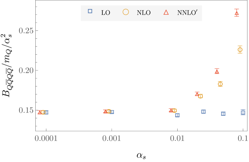
Figure 1: Tetraquark binding energies divided by $m_{Q}\alpha_{s}^{2}$ as functions of $\alpha_{s}$. Error bars show combined statistical and fitting systematic uncertainties computed from GFMC results as described in the main text with different colors and markers corresponding to different orders of pNRQCD and NLO-NNLO^′ points horizontally offset for clarity.

Tetraquark binding energy results — To probe the existence of bound tetraquarks for asymptotically large quark masses, which correspond to $\alpha_{s}(\mu_{p})\ll 1$, we performed VMC calculations with $10^{-4}\leq\alpha_{s}\leq 0.1$ at LO, NLO, and NNLO^′. We find that $b/a\approx 5$ leads to near-optimal variational bounds for the family of trial wavefunctions in Eq. (13) and that $\Delta E_{QQ\overline{Q}\overline{Q}}<2\Delta E_{Q\overline{Q}}$, indicating the precense of bound fully-heavy tetraquark states over this range of $\alpha_{s}$.

Subsequent GFMC calculations are used to improve on these variational bounds. Application of $e^{-H\tau}$ effectively suppresses excited-state effects if $\tau$ is larger than the excitation energy. For a Coulombic potential, this gap is expected to be of order $\delta=m_{Q}/(C_{F}\alpha_{s})^{2}$. By taking our GFMC parameters to scale as $\delta\tau\propto 1/(\alpha_{s}^{2}m_{Q})$, we achieve $\tau>\delta$ even for calculations of $\alpha_{s}=10^{-4}$. We find that excited-state effects are present for $\tau\lesssim\delta$ with apparent plateaus in

$$\Delta E(\tau)=\left<\Psi_{T}\vphantom{He^{-H\tau}\psi_{T}}\right|He^{-H\tau}\left|\psi_{T}\vphantom{\Psi_{T}He^{-H\tau}}\right>,$$ (15)

visible for $\tau$ larger than $0.5-2$ times $\delta$ for all $\alpha_{s}$ studied as shown in the supplemental material. We fit the large-$\tau$ behavior of $\Delta E(\tau)$ to constants using bootstrap methods, shrinkage Ledoit and Wolf (2004), and model averaging over fit ranges Jay and Neil (2021) as detailed in Ref. Assi and Wagman (2023).

These GFMC binding energy results are shown in Fig. 1 and indicate that LO, NLO, and NNLO^′ results give consistent binding energies at the percent level for $\alpha_{s}\lesssim 0.01$. In this regime, we find that the tetraquark binding energy is approximately proportional to $\alpha_{s}^{2}$ and consistent with

$$\begin{split}B_{QQ\overline{Q}\overline{Q}}&=-\Delta E_{QQ\overline{Q}\overline{Q}}+2\Delta E_{Q\overline{Q}}\\ &=0.148(2)\alpha_{s}^{2}m_{Q}.\end{split}$$ (16)

This demonstrates that bound fully-heavy tetraquark states exist at asymptotically heavy quark masses where $1/m_{Q}$-suppressed effects can be neglected. Note that this has the same scaling as the LO quarkonium result $B_{Q\overline{Q}}=C_{F}^{2}\alpha_{s}^{2}m_{Q}/4$ but with a factor of 0.166(2) smaller binding energy per particle.

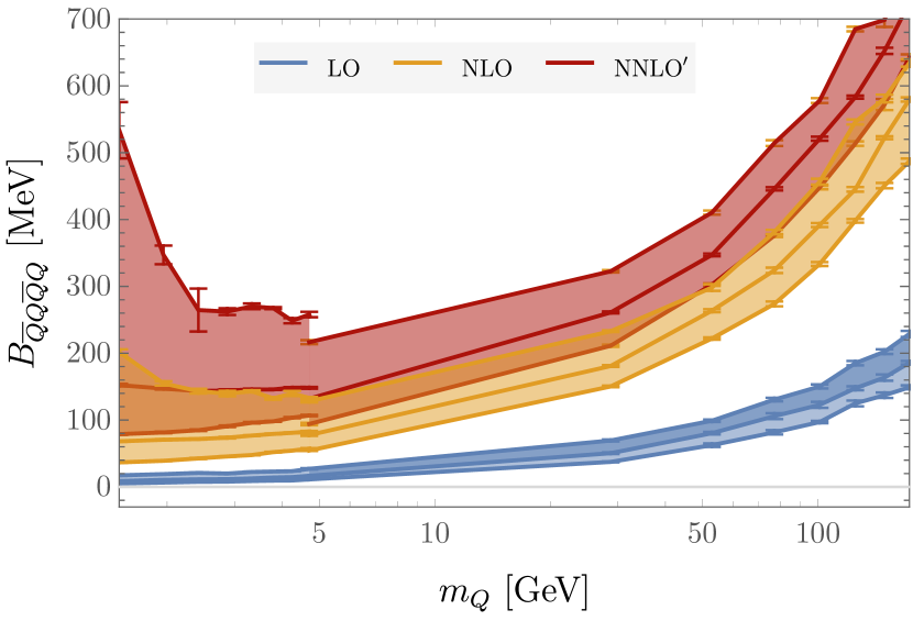
Figure 2: Tetraquark binding energies for equal-mass quarks with masses ranging from $m_{c}$ to $m_{t}$. Shaded bands connect results with renormalization scale choices $\mu\in\{\mu_{p},2\mu_{p},\mu_{p}/2$} at each pNRQCD order indicated.

To study tetraquarks over the range of $m_{Q}$ relevant for heavy quarks in QCD, we perform GFMC calculations using the same trial wavefunction with $b/a\approx 5$ over masses ranging from $m_{c}$ to $m_{t}$. We take $\alpha_{s}(M_{Z})=0.1184(7)$ and compute the Landau pole scale $\Lambda_{\rm QCD}$ and matching across quark mass thresholds as described in Ref. Bethke (2009). We perform GFMC calculations with $\mu\in\{\mu_{p},\mu_{p}/2,2\mu_{p}\}$ to study the renormalization scale dependence of our results. Non-zero tetraquark binding energies are obtained at high statistical significance over the full range of masses and renormalization scales studied, as shown in Fig. 2.

To predict the masses and binding energies of physical tetraquarks, we use the $b$ and $c$ quark poles masses determined in Ref. Assi and Wagman (2023) by tuning to reproduce experimental results for spin-averaged $(J/\psi,\eta_{c})$ and $(\Upsilon,\eta_{b})$ masses. We validate our approximations by predicting spin-averaged $(B_{c},B_{c}^{*})$ masses that are compared with experimental Workman et al. (2022) and lattice QCD Mathur et al. (2018) results in Table 1. Our pNRQCD results converge slowly towards experimental and lattice QCD results with $38(7)$ MeV (corresponding to 0.6%) deviations present at NNLO^′ . Predictions for equal-mass $T_{bb\overline{b}\overline{b}}$ and $T_{cc\overline{c}\overline{c}}$ tetraquarks, as well as unequal-mass tetraquarks involving combinations of $b$ and $c$ quarks, are shown in Table 2. To obtain precise results for $B_{QQ\overline{Q}\overline{Q}}$, we compute correlated differences between $\Delta E_{QQ\overline{Q}\overline{Q}}$ and $2\Delta E_{Q\overline{Q}}$ by computing the latter using the same Monte Carlo ensemble proportional to $|\Psi_{T}^{Q_{i}\overline{Q}_{j}Q_{k}\overline{Q}_{l}}|^{2}$ as used for the tetraquark calculation and only including the terms in the potential appearing for a product of two non-interacting mesons. For unequal mass tetraquarks $\mu_{p}$ is defined as $\mu_{p}=4\alpha_{s}(\mu_{p})m_{\text{red}}$ in terms of the reduced mass $m_{\text{red}}=(n_{b}+n_{c})m_{b}m_{c}/(n_{b}m_{b}+n_{c}m_{c})$ where $n_{b}$ ($n_{c}$) is the number of constituents with mass $m_{b}$ ($m_{c}$). Differences between tetraquark energy results for different pNRQCD orders are small fractions of $M_{QQ\overline{Q}\overline{Q}}$ but large fractions of $B_{QQ\overline{Q}\overline{Q}}$; however, the existence of non-zero $B_{QQ\overline{Q}\overline{Q}}$ is a robust prediction for all orders and flavor combinations studied.

Our NLO and NNLO^′  results for $b$ and $c$ quark masses using a range of renormalization scales suggest that fully-heavy tetraquarks have binding energies of 50-200 MeV. The inclusion of higher order and $1/m_{Q}$-suppressed effects will affect these results, but a conservative estimate of the size of these effects obtained by doubling the difference between pNRQCD and experiment/lattice for the $(B_{c},B_{c}^{*})$ mass (which assumes zero cancellations between higher-order effects on $\Delta E_{QQ\overline{Q}\overline{Q}}$ and $\Delta E_{Q\overline{Q}}$) suggests that they will not alter the conclusion that fully-heavy $b$ and $c$ tetraquark bound states exist.

Mesons	Order	$M_{Q\bar{Q}}$ [GeV]	$M_{Q\bar{Q}}^{\text{exp/lat}}$ [GeV] Workman et al. (2022); Mathur et al. (2018)
$(B_{c},B_{c}^{*})$	LO NLO NNLO	6.26505 6.273(2) 6.279(3)	6.317(6)

Table 1: Spin-averaged ${}^{1}S$ masses for $b\overline{c}/c\overline{b}$ mesons at each order of pNRQCD indicated. The rightmost column shows $1/4$ times the experimentally measured spin-0 $B_{c}$ mass Workman et al. (2022) plus $3/4$ times the spin-1 $B_{c}^{*}$ mass (which has not yet been experimentally determined) from lattice QCD Mathur et al. (2018).

Tetraquarks	Order	$M_{Q\bar{Q}Q\bar{Q}}$ [GeV]	$B_{Q\bar{Q}Q\bar{Q}}$ [MeV]
$T_{cc\overline{c}\overline{c}}$	LO NLO NNLO′	6.1276(3) 6.078(2) 6.018(3)	16.6(4) 67.9(1) 144(2)
$T_{cc\overline{c}\overline{b}}/T_{bc\overline{c}\overline{c}}$	LO NLO NNLO′	9.294(3) 9.312(4) 9.259(5)	23.0(4) 72(2) 139(2)
$T_{bb\overline{c}\overline{c}}/T_{cc\overline{b}\overline{b}}$	LO NLO NNLO′	12.503(1) 12.457(4) 12.386(3)	23.7(4) 79(2) 157(3)
$T_{bc\overline{b}\overline{c}}$	LO NLO NNLO′	12.471(5) 12.417(5) 12.354(6)	19.5(8) 69(2) 139(2)
$T_{bb\overline{b}\overline{c}}/T_{bc\overline{b}\overline{b}}$	LO NLO NNLO′	15.652(6) 15.50(2) 15.37(7)	27.9(7) 87(2) 169(4)
$T_{bb\overline{b}\overline{b}}$	LO NLO NNLO′	18.8693(5) 18.8207(6) 18.7598(6)	31.2(6) 83.6(1) 151(1)

Table 2: Predictions for tetraquark masses and binding energies for all combinations of tetraquarks involving only $b$ and $c$ quarks at each order of pNRQCD indicated. Pairs of tetraquarks in the same row have identical binding energies in our calculations due to charge conjugation.

Evidence for an additional near-threshold state — Increasing the ratio of $b/a$ away from the optimal value of $b/a\sim 5$ obtained through VMC calculations to values of $b/a\sim 100$ leads to larger but much more precise Hamiltonian matrix elements as shown in Fig. 3 for the example of the LO potential with a quark mass corresponding to $m_{b}$. States with zero-variance Hamiltonian matrix elements are in one-to-one correspondence with energy eigenstates. The observation of a trial wavefunction providing low-variance Hamiltonian matrix elements that are significantly larger than those obtained with other trial wavefunctions therefore suggests the presence of an excited state in the spectrum with a wavefunction that is well approximated by Eq. (13) with $b/a\sim 100$.

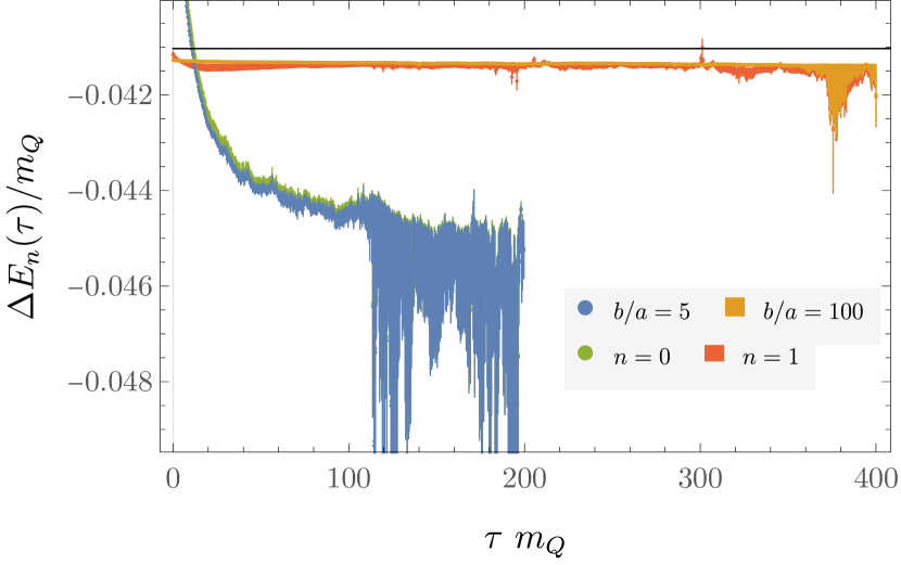
Figure 3: GFMC results for $T_{bb\overline{b}\overline{b}}$ $\Delta E(\tau)$ at LO using two different values of the trial wavefunction parameter $b/a$ compared with the analogous results $\Delta E_{n}(\tau)$ from approximate energy eigenstates obtained by solving a GEVP. The black line shows the two-meson threshold $2\Delta E_{Q\overline{Q}}/m_{Q}$; matrix elements below this line indicate bound tetraquark states.

In order to test whether trial wavefunctions with small and large $b/a$ are overlapping with two or more energy eigenstates, we computed a matrix of two-point correlation functions,

$$C_{IJ}(\tau)=\left<\Psi_{I}\vphantom{e^{-H\tau}\Psi_{J}}\right|e^{-H\tau}\left|\Psi_{J}\vphantom{\Psi_{I}e^{-H\tau}}\right>,$$ (17)

with different initial- and final-state trial wavefunctions for $I\neq J$ using GFMC methods by performing Metropolis sampling with one of the wavefunctions and then including appropriate reweighting factors.. We then construct approximate energy eigenstates by solving a generalized eigenvalue problem (GEVP) Fox et al. (1982); Michael and Teasdale (1983); Lüscher and Wolff (1990); Blossier et al. (2009)

$$C_{IJ}(\tau_{\text{ref}})v_{Jn}=\lambda_{n}C_{IJ}(\tau_{0})v_{Jn},$$ (18)

to obtain the generalized eigenvalues $\lambda_{n}(\tau_{\text{ref}},\tau_{0})$ and eigenvectors $v_{Jn}(\tau_{\text{ref}},\tau_{0})$ at a variety of initial and reference imaginary times $\tau_{0}$ and $\tau_{\text{ref}}$ (dependence on these scales is suppressed in Eq. (18) for brevity). The eigenvectors can also be used as a change-of-basis matrix that is applied to Hamiltonian matrix elements as

$$\Delta E_{n}(\tau)=\frac{v_{In}^{*}\left<\Psi_{I}\vphantom{He^{-H\tau}\Psi_{J}}\right|He^{-H\tau}\left|\Psi_{J}\vphantom{\Psi_{I}He^{-H\tau}}\right>v_{Jn}}{v_{Kn}^{*}C_{KL}(\tau)v_{Ln}},$$ (19)

which equals $\Delta E_{n}$ plus exponentially suppressed excited-state effects under the assumption that the set of states used to construct the correlation function matrix overlaps with the lowest energy eigenstates. We compute statistical and systematic uncertainties from solving the GEVP at a wide range of $\tau_{0}$ and $\tau_{\text{ref}}$ by taking different choices for these parameters for each bootstrap sample.

Results with the LO potential and $m_{Q}=m_{b}$ for solving the GEVP for a $2\times 2$ matrix of correlation functions involving wavefunctions $\Psi_{I}$ with $I\in\{1,2\}$ corresponding to $b/a\in\{5,100\}$ are shown in Fig. 3. Two approximately orthogonal states can be resolved with high precision and results for $n=0$ ($n=1$) are consistent with results using a single trial wavefunction with $b/a=5$ ($b/a=100$). The resulting ground-state energy is $19(1)$ MeV below the two-meson threshold, while the excited-state energy is $1.7(2)$ MeV below the two-meson threshold. This indicates the presence of a second $T_{bb\overline{b}\overline{b}}$ bound state very close to threshold.

We further solve the GEVP for a $3\times 3$ matrix of correlation functions involving wavefunctions $\Psi_{I}$ with $I\in\{1,2,3\}$ corresponding to $b/a\in\{5,50,100\}$. In this case, the determinant and eigenvalues of $C_{IJ}(\tau)$ cannot be resolved from zero at $1\sigma$ precision. This suggests that there is no third energy eigenstate with a large overlap with this set of trial wavefunctions. However, it does not exclude the possibility of other bound excited states.

Beyond LO, quarkonium masses cannot be computed analytically, and the location of the two-meson threshold includes statistical uncertainties. Precise GFMC results using $b/a=100$ wavefunctions are obtained using the correlated difference strategy described above that correspond to tetraquark binding energies of $4.7(1)$ MeV at NLO and $12.0(4)$ MeV at NNLO^′. However, performing a complete GEVP analysis using such correlated differences is not straightforward, and without exploiting these correlations our statistical uncertainties are too large to distinguish whether this near-threshold state is bound. Corrections from higher-order potentials suppressed by $1/m_{Q}$ could also plausibly change whether this near-threshold state is bound or unbound; however, they should not affect the existence of an additional near-threshold energy level because energies depend smoothly on the parameters of the potential.

Discussion — In this work, we have used quantum Monte Carlo methods to determine the ground-state energies of four heavy-quark systems in pNRQCD, a systematically improvable EFT of QCD. Our results robustly demonstrate that tetraquarks exist as stable QCD bound states for asymptotically heavy quark masses. Calculations for physical $b$ and $c$ quark masses further suggest the existence of tetraquark states that are bound by 50-200 MeV.

These results motivate experimental searches for tetraquark states at the LHC and other colliders. Signals for the observations of such tetraquark states have been studied theoretically Anwar et al. (2018); Eichten and Liu (2017); Vega-Morales and Vega-Morales (2017); Esposito et al. (2021), and hints of possible detection of a $T_{cc\overline{c}\overline{c}}$ state have recently been seen at the LHC Aaij et al. (2020); Hayrapetyan et al. (2023). Although a search for $T_{bb\overline{b}\overline{b}}$ bound states decaying through virtual $\Upsilon$ states did not provide evidence for their existence Aaij et al. (2018), this could be due to a small branching fraction for $T_{bb\overline{b}\overline{b}}\rightarrow\Upsilon\mu\mu$ Esposito and Polosa (2018).

Previous lattice NRQCD calculations have not found evidence for bound $T_{bb\overline{b}\overline{b}}$ tetraquarks Hughes et al. (2018); however, the results of these studies may be affected by systematic uncertainties, including excited-state effects and discretization effects that were not explicitly studied. In particular, we have found evidence for a second near-threshold bound state in pNRQCD that has a significant overlap with the same family of molecular trial wavefunctions with a large overlap with the ground state. If an interpolating operator used in Ref. Hughes et al. (2018) has significant overlap with this near-threshold state, or with unbound finite-volume analogs of scattering states, it would be challenging to detect any evidence for the existence of a bound state using computationally accessible imaginary times. Future lattice NRQCD studies should apply variational methods to a set of multiple interpolating operators to explore this possibility. Such studies could also explicitly test the alternative possibility that $1/m_{Q}$-suppressed effects explain the differences between our results and those of Ref. Hughes et al. (2018) by performing calculations with and without $1/m_{Q}$-suppressed effects included.

Applying QMC methods to pNRQCD further opens a new avenue for studying newly discovered or undiscovered exotic hadrons using computationally efficient and systematically improvable EFT approximations to QCD. Future studies will provide insight into the structure of exotic hadrons comprised of heavy quarks and illuminate which aspects of the complex dynamics of QCD are essential for forming multi-hadron bound states and resonances.

I Acknowledgments

We thank Matthew Baumgart, Nora Brambilla, William Detmold, Majid Ekhterachian, Anthony Grebe, Stefan Stelzl, Daniel Stolarski, Antonio Vairo, and Ruth Van de Water for helpful discussions and insightful comments. This manuscript has been authored by Fermi Research Alliance, LLC under Contract No. DE-AC02-07CH11359 with the U.S. Department of Energy, Office of Science, Office of High Energy Physics. This work was performed in part at the Aspen Center for Physics, which is supported by National Science Foundation grant PHY-2210452.

II Supplemental material

II.1 Direct sampling

Quantum Monte Carlo methods involve evaluating integrals over the spatial coordinates for all spin, and in our case, color, components of particles in a many-body system. Heavy-quark spin components decouple at leading order in $1/m_{Q}$, and this work, therefore, requires evaluating $3N_{Q}$-dimensional integrals such as Eq. (7) for systems with $N_{Q}$ heavy quarks/antiquarks with Monte Carlo methods. This approach stochastically approximates the integral, with the trial wavefunction’s magnitude forming the basis for a probability distribution:

$$\mathcal{P}(\boldsymbol{R})\propto\Psi_{T}^{i_{1}\ldots i_{N_{q}}}(\boldsymbol{R})\Psi_{T}^{i_{1}\ldots{i}_{N_{q}}}(\boldsymbol{R})^{*},$$ (20)

where $i_{1},\ldots,i_{N_{Q}}$ are the wavefunction color indices. Ratios of wavefunction integrals such as Eq. (7) can be described as expectation values $\left<\cdot\right>$ of coordinates $\boldsymbol{R}$ sampled from this distribution,

$$\left<\Psi_{T}\vphantom{H\Psi_{T}}\right|H\left|\Psi_{T}\vphantom{\Psi_{T}H}\right>=\left<\frac{\Psi_{T}(\boldsymbol{R})^{*}H(\boldsymbol{R})\Psi_{T}(\boldsymbol{R})}{|\Psi_{T}(\boldsymbol{R})|^{2}}\right>,$$ (21)

Note that the wavefunction factors cancel from Eq. (21) for terms involving the potential, but the action of the kinetic term on the wavefunction leads to factors of $(\nabla^{2}\Psi_{T})/\Psi_{T}$.

For quarkonium wavefunctions, it is straightforward to sample from Eq. (20) using a simple iterative updating scheme in which, for instance, the coordinates $\boldsymbol{R}_{i}$ at each step are replaced by coordinates $\boldsymbol{R}_{i+1}=\varepsilon\boldsymbol{\xi}$ where $\boldsymbol{\xi}$ is a three-vector of zero-norm unit-variance Gaussian random variable and $\varepsilon$ is a tunable step size. These updates are accepted as elements of a Markov chain with probability $w_{i+1}=\mathcal{P}(\boldsymbol{R}_{i+1})/\mathcal{P}(\boldsymbol{R}_{i}),$ and rejected otherwise. Elements of such a Markov chain are correlated with one another, and obtaining approximately independent random variables requires several updates that are larger than the autocorrelation time. Samples drawn with step size $\varepsilon\approx 2/(\alpha_{V}m_{Q})$ can achieve manageable autocorrelation times of order 10 for quarkonium over a wide range of $m_{Q}$ as described in Ref. Assi and Wagman (2023). Similar results are found when applying this scheme to tetraquark wavefunctions that are relatively compact, $b/a\lesssim 5$. Autocorrelation times increase with increasing $b/a$; however, they are undesirably large for very diffuse molecular wavefunctions with $b/a\gtrsim 10$. These autocorrelations lead to significant statistical uncertainties for large $b/a$.

Alternative approaches in which a distribution approximating $\mathcal{P}(\boldsymbol{R})$ that can be directly sampled from are used to propose new Markov chain elements have been shown to successfully reduce large autocorrelations in lattice field theory applications Albergo et al. (2019). Machine learning techniques are often used to expressively parameterize distributions that can be trained to approximate complicated distributions, but in our case, the relative simplicity of our trial wavefunctions defining $\mathcal{P}(\boldsymbol{R})$ allows us to construct a simple two-parameter distribution as described below that is effective for direct sampling.

We build our direct sampling distribution $Q(\boldsymbol{R})$ approximating $\mathcal{P}(\boldsymbol{R})$ from functions of exponentially distributed random variables. Random variables can be drawn from an exponential distribution $\mathcal{P}(x)=e^{-\lambda x}/\lambda$ by first generating uniform random variables $z\in[0,1]$ and then applying the change of variables $x=-1/\lambda\ln z$, which has Jacobean $\frac{\partial x}{\partial z}=\mathcal{P}(x)$. The coordinates $\boldsymbol{r}_{i}$ and $\boldsymbol{r}_{j}$ for the quark and antiquark in each color-singlet quarkonium pair in our molecular trial wavefunction are defined from exponentially distributed random variables $x_{ij}^{1},x_{ij}^{2},x_{ij}^{3}$ with width $\lambda$ and a second set of exponentially distributed variables $\rho_{ij}^{1},\rho_{ij}^{2},\rho_{ij}^{3}$ with width $L$. These variables are multiplied by a random sign $\pm 1$ and then taken to be the Cartesian components of vectors $\boldsymbol{x}_{ij}$ and $\boldsymbol{\rho}_{ij}$ that define the relative and center-of-mass position of this quarkonium pair as $\boldsymbol{r}_{i}=\boldsymbol{x}_{ij}+\boldsymbol{\rho}_{ij}$, $\boldsymbol{r}_{j}=-\boldsymbol{x}_{ij}+\boldsymbol{\rho}_{ij}$. To fix the total center-of-mass position to zero, the shift for the second quarkonium pair is defined as $\boldsymbol{r}_{34}=-\boldsymbol{\rho}_{12}$. The resulting probability distribution is

$$Q(\boldsymbol{R})=\frac{1}{\lambda^{6}L^{3}}\prod_{\alpha=1}^{3}e^{-\lambda|x_{12}^{\alpha}|}e^{-\lambda|x_{34}^{\alpha}|}e^{-L|\rho_{12}^{\alpha}|}.$$ (22)

In our direct sampling approach, we construct a Markov chain in which each new element $\boldsymbol{R}_{i+1}$ is sampled from $Q(\boldsymbol{R}_{i+1})$ with no reference to $\boldsymbol{R}_{i}$. Correlations between Markov chain elements only enter through the acceptance probabilities for adding a proposed element to the Markov chain, which are Albergo et al. (2019)

$$w_{i+1}=\frac{\mathcal{P}(\boldsymbol{R}_{i+1})}{\mathcal{P}(\boldsymbol{R}_{i})}\left[\frac{Q(\boldsymbol{R}_{i})}{Q(\boldsymbol{R}_{i+1})}\right].$$ (23)

This acceptance probability corrects for the approximation of sampling from $Q(\boldsymbol{R})$ instead of $\mathcal{P}(\boldsymbol{R})$. For a poor approximation with $w_{i+1}\ll 1$, many updates will be required to generate approximately independent samples, while for an approximation with $w_{i+1}\approx 1$, all updates will be approximately independent and autocorrelation times will be negligible.

We find that taking $\lambda=a/4$ and $L=b/12$ leads to a direct sampling scheme with Metropolis acceptance ratios of 0.4-0.8 over the full range of $\alpha_{s}$ studied in this work. Results using this direct sampling scheme are consistent with those obtained using a simple iterative updating scheme for small $b/a$ and successfully avoid rapid growth in autocorrelation times with increasing $b/a$.

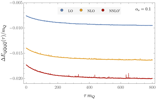
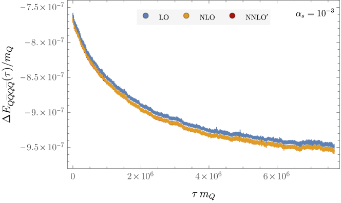
Figure 4: Matrix elements of the pNRQCD Hamiltonian for fully-heavy tetraquark states with $\alpha_{s}=0.1,10^{-3}$.

II.2 GFMC results

In our GFMC calculations, we ensure that $\tau$ is greater than the energy gap between the ground and excited state energy, which translates to $N_{\tau}\delta\tau/m_{Q}>2/(C_{F}\alpha_{s})^{2}$ with statistical ensembles of size $N_{\text{walkers}}=10,000$. In particular we take $N_{\tau}=500$ and $\delta\tau/m_{Q}=0.4$ for all the physical quark mass results shown in Tables 1 and 2 as well as the mass scan in Fig. 2. For the small $\alpha_{s}$ scan in Fig. 1, we again use $N_{\tau}=500$ and increase $\delta\tau$ to maintain $\tau>2/(C_{F}\alpha_{s})^{2}$ and for example for $\alpha_{s}=10^{-4}$ for which we take $\delta\tau/m_{Q}=4\times 10^{6}$.

In our GFMC calculations, we take the correlated difference between the effective mass of the tetraquark system and the associated two-meson system to determine the tetraquark binding energy. These two systems are not necessarily independent, and thus, the correlated difference enhances the statistical precision of GFMC results. In order to use the same $\Psi_{T}$ for the two-meson system, we do one GFMC calculation with the full potential and another with the so-called product potential. The product potential is as given in Eq. (5) except solely including potential terms involving the intra-meson coordinate diffs $r_{12}$ and $r_{34}$. To obtain the correlated difference, we use the same $\Psi_{T}$ and random seed to generate the same ensembles of walkers used for the full Hamiltonian and for a product Hamiltonian. This allows us to compute the correlated difference between the energies from the full and product Hamiltonian with the same trial state, which leads to the binding energies we present.

GFMC effective masses and binding energies using the trial wavefunctions $\Psi_{T}(\boldsymbol{r}_{1\ldots 4})$ are shown in Figs. 4 and 5, respectively. We present systems with constituent quark masses corresponding to $\alpha_{s}(\mu_{p})=10^{-1}$ and $\alpha_{s}(\mu_{p})=10^{-3}$ using the renormalization scale choice $\mu_{p}=4\alpha_{s}(\mu_{p})m_{Q}$. We further studied a range of smaller $\delta\tau$ and larger $N_{\tau}$ to verify that Trotterization effects are negligible for the full range of scales studied here. Slightly less imaginary-time evolution is required to achieve ground-state saturation at a given level of precision for LO versus higher orders in pNRQCD.

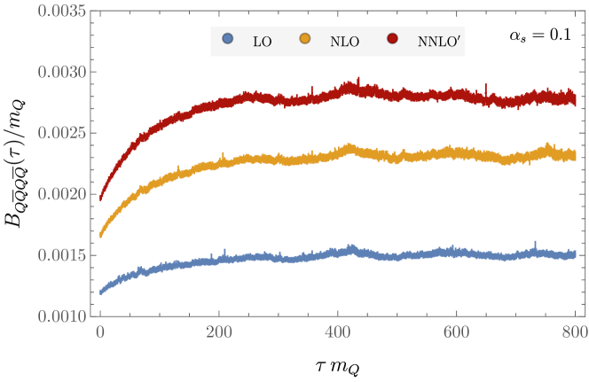
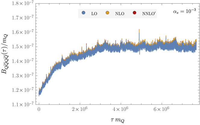
Figure 5: Correlated differences between tetraquark Hamiltonian matrix elements and two time quarkonium matrix elements with $\alpha_{s}=0.1,10^{-3}$ .

References

- Jaffe (1977) R. L. Jaffe, Phys. Rev. D 15, 267 (1977).
- Brambilla et al. (2020) N. Brambilla, S. Eidelman, C. Hanhart, A. Nefediev, C.-P. Shen, C. E. Thomas, A. Vairo, and C.-Z. Yuan, Phys. Rept. 873, 1 (2020), arXiv:1907.07583 [hep-ex] .
- Chen et al. (2023) H.-X. Chen, W. Chen, X. Liu, Y.-R. Liu, and S.-L. Zhu, Rept. Prog. Phys. 86, 026201 (2023), arXiv:2204.02649 [hep-ph] .
- Workman et al. (2022) R. L. Workman et al. (Particle Data Group), PTEP 2022, 083C01 (2022).
- Drenska et al. (2010) N. Drenska, R. Faccini, F. Piccinini, A. Polosa, F. Renga, and C. Sabelli, Riv. Nuovo Cim. 33, 633 (2010), arXiv:1006.2741 [hep-ph] .
- Brambilla et al. (2011) N. Brambilla et al., Eur. Phys. J. C 71, 1534 (2011), arXiv:1010.5827 [hep-ph] .
- Brambilla et al. (2014) N. Brambilla et al., Eur. Phys. J. C 74, 2981 (2014), arXiv:1404.3723 [hep-ph] .
- Esposito et al. (2015) A. Esposito, A. L. Guerrieri, F. Piccinini, A. Pilloni, and A. D. Polosa, Int. J. Mod. Phys. A 30, 1530002 (2015), arXiv:1411.5997 [hep-ph] .
- Lebed et al. (2017) R. F. Lebed, R. E. Mitchell, and E. S. Swanson, Prog. Part. Nucl. Phys. 93, 143 (2017), arXiv:1610.04528 [hep-ph] .
- Chen et al. (2016) H.-X. Chen, W. Chen, X. Liu, and S.-L. Zhu, Phys. Rept. 639, 1 (2016), arXiv:1601.02092 [hep-ph] .
- Liu et al. (2019) Y.-R. Liu, H.-X. Chen, W. Chen, X. Liu, and S.-L. Zhu, Prog. Part. Nucl. Phys. 107, 237 (2019), arXiv:1903.11976 [hep-ph] .
- Bicudo and Wagner (2013) P. Bicudo and M. Wagner (European Twisted Mass), Phys. Rev. D 87, 114511 (2013), arXiv:1209.6274 [hep-ph] .
- Brown and Orginos (2012) Z. S. Brown and K. Orginos, Phys. Rev. D 86, 114506 (2012), arXiv:1210.1953 [hep-lat] .
- Bicudo et al. (2015) P. Bicudo, K. Cichy, A. Peters, B. Wagenbach, and M. Wagner, Phys. Rev. D 92, 014507 (2015), arXiv:1505.00613 [hep-lat] .
- Francis et al. (2017) A. Francis, R. J. Hudspith, R. Lewis, and K. Maltman, Phys. Rev. Lett. 118, 142001 (2017), arXiv:1607.05214 [hep-lat] .
- Francis et al. (2019) A. Francis, R. J. Hudspith, R. Lewis, and K. Maltman, Phys. Rev. D 99, 054505 (2019), arXiv:1810.10550 [hep-lat] .
- Junnarkar et al. (2019) P. Junnarkar, N. Mathur, and M. Padmanath, Phys. Rev. D 99, 034507 (2019), arXiv:1810.12285 [hep-lat] .
- Leskovec et al. (2019) L. Leskovec, S. Meinel, M. Pflaumer, and M. Wagner, Phys. Rev. D 100, 014503 (2019), arXiv:1904.04197 [hep-lat] .
- Hudspith et al. (2020) R. J. Hudspith, B. Colquhoun, A. Francis, R. Lewis, and K. Maltman, Phys. Rev. D 102, 114506 (2020), arXiv:2006.14294 [hep-lat] .
- Bicudo et al. (2021) P. Bicudo, A. Peters, S. Velten, and M. Wagner, Phys. Rev. D 103, 114506 (2021), arXiv:2101.00723 [hep-lat] .
- Padmanath and Prelovsek (2022) M. Padmanath and S. Prelovsek, Phys. Rev. Lett. 129, 032002 (2022), arXiv:2202.10110 [hep-lat] .
- Meinel et al. (2022) S. Meinel, M. Pflaumer, and M. Wagner, Phys. Rev. D 106, 034507 (2022), arXiv:2205.13982 [hep-lat] .
- Bicudo (2022) P. Bicudo, (2022), arXiv:2212.07793 [hep-lat] .
- Lyu et al. (2023) Y. Lyu, S. Aoki, T. Doi, T. Hatsuda, Y. Ikeda, and J. Meng, Phys. Rev. Lett. 131, 161901 (2023), arXiv:2302.04505 [hep-lat] .
- Aoki et al. (2023) T. Aoki, S. Aoki, and T. Inoue, Phys. Rev. D 108, 054502 (2023), arXiv:2306.03565 [hep-lat] .
- Padmanath et al. (2023) M. Padmanath, A. Radhakrishnan, and N. Mathur, (2023), arXiv:2307.14128 [hep-lat] .
- Bodwin et al. (1995) G. T. Bodwin, E. Braaten, and G. P. Lepage, Phys. Rev. D 51, 1125 (1995), [Erratum: Phys.Rev.D 55, 5853 (1997)], arXiv:hep-ph/9407339 .
- Caswell and Lepage (1986) W. E. Caswell and G. P. Lepage, Phys. Lett. B 167, 437 (1986).
- Pineda and Soto (1998a) A. Pineda and J. Soto, Nucl. Phys. B Proc. Suppl. 64, 428 (1998a), arXiv:hep-ph/9707481 .
- Pineda and Soto (1998b) A. Pineda and J. Soto, Phys. Rev. D 58, 114011 (1998b), arXiv:hep-ph/9802365 .
- Brambilla et al. (2000) N. Brambilla, A. Pineda, J. Soto, and A. Vairo, Nucl. Phys. B 566, 275 (2000), arXiv:hep-ph/9907240 .
- Pineda (2012) A. Pineda, Prog. Part. Nucl. Phys. 67, 735 (2012), arXiv:1111.0165 [hep-ph] .
- Vijande et al. (2007) J. Vijande, A. Valcarce, and J. M. Richard, Phys. Rev. D 76, 114013 (2007), arXiv:0707.3996 [hep-ph] .
- Berezhnoy et al. (2012) A. V. Berezhnoy, A. V. Luchinsky, and A. A. Novoselov, Phys. Rev. D 86, 034004 (2012), arXiv:1111.1867 [hep-ph] .
- Wu et al. (2018) J. Wu, Y.-R. Liu, K. Chen, X. Liu, and S.-L. Zhu, Phys. Rev. D 97, 094015 (2018), arXiv:1605.01134 [hep-ph] .
- Chen et al. (2017) W. Chen, H.-X. Chen, X. Liu, T. G. Steele, and S.-L. Zhu, Phys. Lett. B 773, 247 (2017), arXiv:1605.01647 [hep-ph] .
- Karliner et al. (2017) M. Karliner, S. Nussinov, and J. L. Rosner, Phys. Rev. D 95, 034011 (2017), arXiv:1611.00348 [hep-ph] .
- Bai et al. (2019) Y. Bai, S. Lu, and J. Osborne, Phys. Lett. B 798, 134930 (2019), arXiv:1612.00012 [hep-ph] .
- Wang and Di (2019) Z.-G. Wang and Z.-Y. Di, Acta Phys. Polon. B 50, 1335 (2019), arXiv:1807.08520 [hep-ph] .
- Hughes et al. (2018) C. Hughes, E. Eichten, and C. T. H. Davies, Phys. Rev. D 97, 054505 (2018), arXiv:1710.03236 [hep-lat] .
- Anwar et al. (2018) M. N. Anwar, J. Ferretti, F.-K. Guo, E. Santopinto, and B.-S. Zou, Eur. Phys. J. C 78, 647 (2018), arXiv:1710.02540 [hep-ph] .
- Brambilla et al. (1999) N. Brambilla, A. Pineda, J. Soto, and A. Vairo, Phys. Lett. B 470, 215 (1999), arXiv:hep-ph/9910238 .
- Kniehl et al. (2002) B. A. Kniehl, A. A. Penin, V. A. Smirnov, and M. Steinhauser, Nucl. Phys. B 635, 357 (2002), arXiv:hep-ph/0203166 .
- Pineda and Yndurain (1998) A. Pineda and F. J. Yndurain, Phys. Rev. D 58, 094022 (1998), arXiv:hep-ph/9711287 .
- Brambilla et al. (2005) N. Brambilla, A. Vairo, and T. Rosch, Phys. Rev. D 72, 034021 (2005), arXiv:hep-ph/0506065 .
- Brambilla et al. (2010) N. Brambilla, J. Ghiglieri, and A. Vairo, Phys. Rev. D 81, 054031 (2010), arXiv:0911.3541 [hep-ph] .
- Brambilla et al. (2013) N. Brambilla, F. Karbstein, and A. Vairo, Phys. Rev. D 87, 074014 (2013), arXiv:1301.3013 [hep-ph] .
- Assi and Wagman (2023) B. Assi and M. L. Wagman, (2023), arXiv:2305.01685 [hep-ph] .
- Jia (2006) Y. Jia, JHEP 10, 073 (2006), arXiv:hep-ph/0607290 .
- Llanes-Estrada et al. (2012) F. J. Llanes-Estrada, O. I. Pavlova, and R. Williams, Eur. Phys. J. C 72, 2019 (2012), arXiv:1111.7087 [hep-ph] .
- Carlson et al. (2015) J. Carlson, S. Gandolfi, F. Pederiva, S. C. Pieper, R. Schiavilla, K. E. Schmidt, and R. B. Wiringa, Rev. Mod. Phys. 87, 1067 (2015), arXiv:1412.3081 [nucl-th] .
- Yan and Blume (2017) Y. Yan and D. Blume, Journal of Physics B: Atomic, Molecular and Optical Physics 50, 223001 (2017).
- Gandolfi et al. (2020) S. Gandolfi, D. Lonardoni, A. Lovato, and M. Piarulli, Front. in Phys. 8, 117 (2020), arXiv:2001.01374 [nucl-th] .
- Anzai et al. (2013) C. Anzai, M. Prausa, A. V. Smirnov, V. A. Smirnov, and M. Steinhauser, Phys. Rev. D 88, 054030 (2013), arXiv:1308.1202 [hep-ph] .
- Pineda and Soto (1999) A. Pineda and J. Soto, Phys. Rev. D 59, 016005 (1999), arXiv:hep-ph/9805424 .
- Kniehl and Penin (1999) B. A. Kniehl and A. A. Penin, Nucl. Phys. B 563, 200 (1999), arXiv:hep-ph/9907489 .
- Toulouse and Umrigar (2007) J. Toulouse and C. J. Umrigar, The Journal of chemical physics 126 (2007).
- Albergo et al. (2019) M. S. Albergo, G. Kanwar, and P. E. Shanahan, Phys. Rev. D 100, 034515 (2019), arXiv:1904.12072 [hep-lat] .
- Wheeler (1946) J. A. Wheeler, Annals N. Y. Acad. Sci. 48, 219 (1946).
- Hylleraas and Ore (1947) E. A. Hylleraas and A. Ore, Phys. Rev. 71, 493 (1947).
- Sharma (1968) R. R. Sharma, Phys. Rev. 171, 36 (1968).
- Ho (1986) Y. K. Ho, Phys. Rev. A 33, 3584 (1986).
- Frolov and Smith (1996) A. M. Frolov and V. H. Smith, J. Phys. B 29, L433 (1996).
- Czarnecki (2009) A. Czarnecki, Nucl. Phys. A 827, 541c (2009).
- Aslam et al. (2021) M. J. Aslam, W. Chen, A. Czarnecki, S. R. Mir, and M. Mubasher, Phys. Rev. A 104, 052803 (2021), arXiv:2108.06785 [hep-ph] .
- Cassidy et al. (2005) D. B. Cassidy, S. H. M. Deng, R. G. Greaves, T. Maruo, N. Nishiyama, J. B. Snyder, H. K. M. Tanaka, and A. P. Mills, Jr, Phys. Rev. Lett. 95, 195006 (2005).
- Cassidy et al. (2012) D. B. Cassidy, T. H. Hisakado, H. W. K. Tom, and A. P. Mills, Phys. Rev. Lett. 108, 133402 (2012).
- Dyson (1952) F. J. Dyson, Physical Review 85, 631 (1952).
- Pineda and Soto (1998c) A. Pineda and J. Soto, Physical Review D 59, 016005 (1998c).
- Ledoit and Wolf (2004) O. Ledoit and M. Wolf, Journal of Multivariate Analysis 88, 365 (2004).
- Jay and Neil (2021) W. I. Jay and E. T. Neil, Phys. Rev. D 103, 114502 (2021), arXiv:2008.01069 [stat.ME] .
- Bethke (2009) S. Bethke, Eur. Phys. J. C 64, 689 (2009), arXiv:0908.1135 [hep-ph] .
- Mathur et al. (2018) N. Mathur, M. Padmanath, and S. Mondal, Phys. Rev. Lett. 121, 202002 (2018), arXiv:1806.04151 [hep-lat] .
- Fox et al. (1982) G. Fox, R. Gupta, O. Martin, and S. Otto, Nucl. Phys. B 205, 188 (1982).
- Michael and Teasdale (1983) C. Michael and I. Teasdale, Nucl. Phys. B 215, 433 (1983).
- Lüscher and Wolff (1990) M. Lüscher and U. Wolff, Nucl. Phys. B 339, 222 (1990).
- Blossier et al. (2009) B. Blossier, M. Della Morte, G. von Hippel, T. Mendes, and R. Sommer, JHEP 04, 094 (2009), arXiv:0902.1265 [hep-lat] .
- Eichten and Liu (2017) E. Eichten and Z. Liu, (2017), arXiv:1709.09605 [hep-ph] .
- Vega-Morales and Vega-Morales (2017) R. Vega-Morales and R. Vega-Morales, (2017), arXiv:1710.02738 [hep-ph] .
- Esposito et al. (2021) A. Esposito, C. A. Manzari, A. Pilloni, and A. D. Polosa, Phys. Rev. D 104, 114029 (2021), arXiv:2109.10359 [hep-ph] .
- Aaij et al. (2020) R. Aaij et al. (LHCb), Sci. Bull. 65, 1983 (2020), arXiv:2006.16957 [hep-ex] .
- Hayrapetyan et al. (2023) A. Hayrapetyan et al. (CMS), (2023), arXiv:2306.07164 [hep-ex] .
- Aaij et al. (2018) R. Aaij et al. (LHCb), JHEP 10, 086 (2018), arXiv:1806.09707 [hep-ex] .
- Esposito and Polosa (2018) A. Esposito and A. D. Polosa, Eur. Phys. J. C 78, 782 (2018), arXiv:1807.06040 [hep-ph] .