pyC²Ray: A flexible and GPU-accelerated Radiative Transfer Framework
for Simulating the Cosmic Epoch of Reionization

Abstract

Detailed modelling of the evolution of neutral hydrogen in the intergalactic medium during the Epoch of Reionization, $5\leq z\leq 20$, is critical in interpreting the cosmological signals from current and upcoming 21-cm experiments such as Low-Frequency Array (LOFAR) and the Square Kilometre Array (SKA). Numerical radiative transfer codes offer the most physically motivated approach for simulating the reionization process. However, they are computationally expensive as they must encompass enormous cosmological volumes while accurately capturing astrophysical processes occurring at small scales ($\lesssim\rm Mpc$). Here, we present pyC²Ray, an updated version of the massively parallel ray-tracing and chemistry code, C²-Ray, which has been extensively employed in reionization simulations. The most time-consuming part of the code is calculating the hydrogen column density along the path of the ionizing photons. Here, we present the Accelerated Short-characteristics Octhaedral RAytracing (ASORA) method, a ray-tracing algorithm specifically designed to run on graphical processing units (GPUs). We include a modern Python interface, allowing easy and customized use of the code without compromising computational efficiency. We test pyC²Ray on a series of standard ray-tracing tests and a complete cosmological simulation with volume size $(349\,\rm Mpc)^{3}$, mesh size of $250^{3}$ and approximately $10^{6}$ sources. Compared to the original code, pyC²Ray achieves the same results with negligible fractional differences, $\sim 10^{-5}$, and a speedup factor of two orders of magnitude. Benchmark analysis shows that ASORA takes a few nanoseconds per source per voxel and scales linearly for an increasing number of sources and voxels within the ray-tracing radii.

[first]organization=Institute of Physics, Laboratory of Astrophysics, Ecole Polytechnique Fédérale de Lausanne (EPFL), addressline=Observatoire de Sauverny, city=Versoix, postcode=1290, country=Switzerland [second]organization=Nordita, KTH Royal Institute of Technology and Stockholm University, addressline=Hannes Alfvéns väg 12, city=Stockholm, postcode=SE-106 91, country=Sweden [third]organization=Astronomy Centre, Department of Physics & Astronomy, addressline=Pevensey III Building, University of Sussex, city=Falmer, Brighton, postcode=BN1 9QH, country=United Kingdom [fourth]organization=The Oskar Klein Centre, Department of Astronomy,, addressline=Stockholm University, AlbaNova, city=Stockholm, postcode=SE-10691, country=Sweden

1 Introduction

The Epoch of Reionization (EoR) is a period of significant interest in the study of our Universe as during the period the appearance of the very first sources of radiation that drove the transition of the intergalactic medium (IGM) from its primordial cold and neutral state, to the present-day hot and highly ionized one (see e.g. Furlanetto et al., 2006; Gorbunov and Rubakov, 2011; Dayal and Ferrara, 2018, for reviews about this era). While indirect observational evidence, such as using high redshift quasar spectra (e.g. Bosman et al., 2022) and the cosmic microwave background (CMB) radiation (e.g. Planck Collaboration et al., 2020), situates the EoR $5\lesssim z\lesssim 30$, its main characteristics are still unknown (Pritchard and Loeb, 2012; Barkana, 2016). The current and upcoming interferometric radio telescopes, such as the Low-Frequency Array (LOFAR; van Haarlem et al., 2013), Hydrogen Epoch of Reionization Array (HERA; DeBoer et al., 2017), Murchison Widefield Array (MWA; Wayth et al., 2018) and Square Kilometre Array (SKA; Mellema et al., 2013), are expected to uncover the details of this key event in cosmic history by detecting the distribution of the redshifted 21-cm signal in the IGM, produced by the spin-flip transitions in neutral hydrogen (Pritchard and Loeb, 2012; Zaroubi, 2013). Accurate modelling of the EoR, which is needed to interpret the observational constraints provided by these experiments, will require performing detailed numerical radiative transfer (RT) and radiation hydrodynamics (RHD) studies on large cosmological scales ($\gtrsim 100$ Mpc). These simulations are challenging because the EoR is a highly non-local process, and the underlying RT equation contains both angular, spatial and frequency dimensions. Various modelling methods exist, a review of which may be found in, e.g. Gnedin and Madau (2022).

Today, most fully numerical RT codes can be divided into two main classes: moment-based and raytracing methods. The former works by considering the hierarchy of angular moments of the RT equation, with some ‘closure relation’ to limit the number of equations to be solved, and treating the radiation as a fluid (e.g. Aubert and Teyssier, 2008). This makes coupling to hydrodynamics natural and, from a computational perspective, has the huge benefit of being independent of the number of ionizing sources in the simulation. On the other hand, moment methods suffer from increased diffusion and unrealistic shadows on optically thick objects. A few examples of codes using moment-based methods are OTVET (Gnedin and Abel, 2001), RAMSES-RT (Rosdahl et al., 2013) and AREPO-RT (Kannan et al., 2019) and although they combine N-body, hydrodynamic and radiative feedback, they tend to be computationally expensive and cannot simulate the required large volumes to model the 21-cm signal measurements (e.g. Mertens et al., 2020; Trott et al., 2020; HERA Collaboration, 2023).

Ray-tracing methods take a more physical approach by casting rays around each source and modelling how the radiation propagates, i.e., is absorbed and scattered, along those rays. The optical depth between the source and the voxel thus determines the ionization rate inside voxels in the simulation domain. This approach has the potential to be more accurate and less diffusive than moment methods but is quite expensive. Thus, in practice, the number of sources that can be considered has been, until recent years, severely limited by the available computational power. C²-Ray (Mellema et al., 2006) and ZEUS-MP (Whalen and Norman, 2006) are two notable examples of ray-tracing-based codes. Both methods have been compared extensively (Iliev et al., 2006), and the advantages of using one over the other have been shown to greatly depend on the problem and context. That being said, it has been argued that accurate modelling of the EoR probed with the current and upcoming 21-cm experiments will require huge simulation volumes ($\gtrsim 200$ Mpc) (Iliev et al., 2014; Kaur et al., 2020; Giri et al., 2023) and therefore encompass a large number of ionizing sources. Developing more efficient RT methods, especially ray-tracing-based ones, is thus highly desirable.

In recent years, there has been a significant surge in the use of general-purpose GPUs for numerical scientific research. These devices have enabled remarkable performance improvements when used to develop applications for problems that can be divided into numerous simple and independent tasks suitable for parallel processing. Consequently, GPU acceleration has been integrated in various astrophysics and cosmological-related tools (e.g. Ocvirk et al., 2016; Potter et al., 2016; Rácz et al., 2019; Cavelan et al., 2020; Wang and Meng, 2021).

Given the success of GPUs in accelerating ray-tracing tasks in computer graphics (Owens et al., 2008; Nickolls and Dally, 2010; Navarro et al., 2014), it is reasonable to explore their application to ray-tracing problems in astrophysics. This motivates our work, where we introduce an Accelerated Short-characteristics Octhaedral RAytracing (ASORA) method designed specifically for C²-Ray. By incorporating GPU methods, we anticipate significant performance enhancements and more efficient simulations, thus opening up new possibilities for research and analysis. Our work aims to bridge the gap between the potential of GPU acceleration and the requirements of ray-tracing tasks in astrophysics, providing a promising avenue for further advancements in this domain.

C²-Ray is a 3D ray-tracing radiative transfer code simulating the EoR initially developed by Mellema et al. (2006) (hereafter: M06). It conserves photons at a voxel-by-voxel level, allowing for large, optically thick grid voxels while maintaining accuracy. The method handles long time steps effectively, surpassing the voxel-crossing time of ionization fronts. It has been extensively used in EoR simulations and updated to include photoheating, X-ray radiation, and helium chemistry (Friedrich et al., 2012; Ross et al., 2017, 2019). C²-Ray is written in Fortran90 and designed for massively parallel systems, utilizing a hybrid MPI and OpenMP approach for efficient radiation propagation. The ionizing sources are distributed over MPI processes, and each of these processes further employs OpenMP threading to propagate radiation in a domain-decomposed manner. The update to C²-Ray in this work comprises two main aspects:

1. GPU-Accelerated ray-tracing Method: The original ray-tracing method used by C²-Ray is not well-suited for GPU parallelization. A new algorithm based on the short-characteristics scheme has been developed to address this limitation. This new method is specifically designed for running on GPUs, enabling efficient computation of column densities, which is the most computationally intensive task in the radiative transfer (RT) method. The GPU implementation leverages massive multi-threading capabilities, resulting in significantly faster performance than the CPU method. This new algorithm is written as a C++/CUDA (e.g. Garland et al., 2008) library with Python bindings for ease of use and integration.

2. Python Wrapper and Interface: While the highly-optimized Fortran90 implementation of C²-Ray excels at computationally intensive tasks, using it for non-time-critical operations, such as physics implementation, interfacing, and I/O operations, is less appealing for new users due to the compiled and statically typed nature of Fortran. To enhance usability and flexibility, the core subroutines of C²-Ray have been wrapped, and a substantial portion of the surrounding code has been rewritten in Python standard libraries. As a result, users can now write an entire C²-Ray simulation as a Python script, making it easier to tweak parameters and add new features without frequently recompiling the core Fortran subroutines.

These updates enable more efficient GPU utilization for critical computations and improve the overall accessibility and versatility of the C²-Ray code through Python scripting and interface enhancements.

This paper is structured as follows. In § (2), we describe how reionization is modelled and summarize how the C²-Ray method works. In § (3), we describe the ray-tracing method used, present our newly developed ASORA algorithm, and briefly discuss the new Python wrapping and interface to the code. Then, in § (4), the updated code is tested on standard idealized situations and benchmarked to determine how much performance improvement is achieved. The source code of pyC²Ray is publicly available at https://github.com/phirling/pyc2ray.

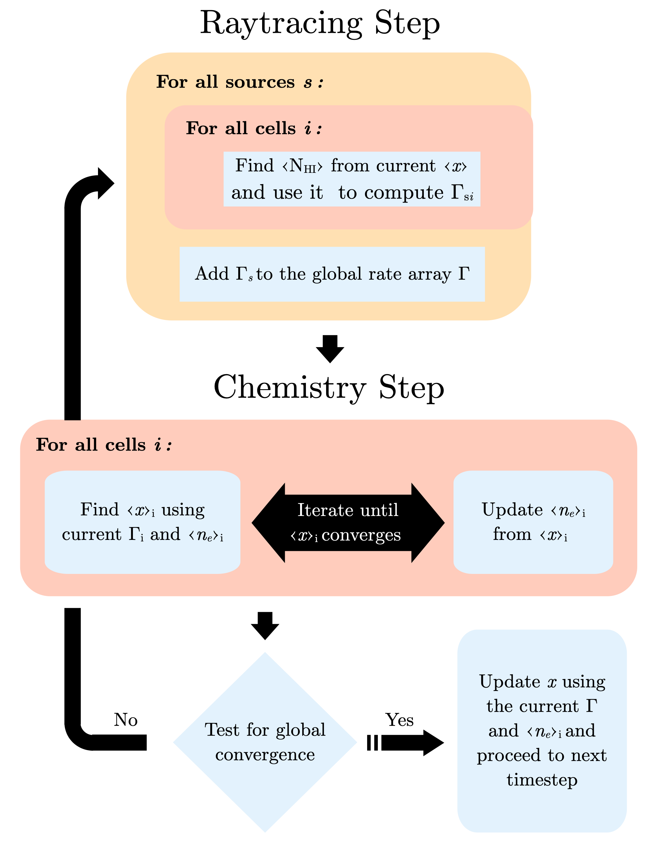
Figure 1: Flowchart representation of the method used by C²-Ray. The figure shows the procedure for a single time-step in which the ionized fraction of hydrogen $x_{\rm HI}$ is evolved for the whole 3D grid. The method can be divided into a "ray-tracing" and a "chemistry" step, and multiple iterations of either typically occur in a single time step.

2 Simulating Cosmic Reionization

To study the EoR, we need to model the time evolution of the ionization state of the intergalactic medium (IGM) within a cosmological framework. This involves solving a system of chemistry equations that track the evolution of the relative abundances of primordial species, such as hydrogen and helium. These equations take into account various physical processes, including photoionization, collisional excitation, recombination, heating and cooling (e.g. Furlanetto et al., 2006).

In this work, we will focus on the simplest case, considering only hydrogen. This choice is justified by the fact that hydrogen constitutes the major part of the IGM. The primary objective of this paper is to present an update to the ray-tracing method, specifically designed for utilization on GPUs. The C²-Ray code incorporates modules to encompass all the aforementioned elements (Friedrich et al., 2012), and we plan to later extend this approach to incorporate more complex chemistry networks. The ionization state of the hydrogen gas is described by the following chemistry equation (e.g. Choudhury and Ferrara, 2006; Choudhury, 2009),

$$\frac{dx_{\rm HII}}{dt}=(1-x_{\rm HII})\left(\Gamma+n_{e}C_{\rm H}(T)\right)-x_{\rm HII}n_{e}\alpha_{\rm H}(T),$$ (1)

where $x_{\rm HII}$ is the fraction of ionized hydrogen and $n_{e}$ is the electron number density, and $C_{\rm H}(T)$ and $\alpha_{\rm H}(T)$ are the collisional ionization and is recombination coefficients for ionized hydrogen and free electrons, at temperature $T$.

C²-Ray uses the On-the-spot (OTS) approximation, which assumes that the diffused photons resulting from recombination to the ground state are reabsorbed locally and, thus, solely accounted for by using a different value for $\alpha_{\rm H}$ (e.g., Ritzerveld, 2005). The photoionization rate $\Gamma$ quantifies the effect of ionizing UV radiation on the gas and is influenced by the distribution of radiation sources. The typical number of these sources during the EoR depends critically on the volume size and minimum mass of source haloes. In the case of a source in every voxel, $N_{s}\sim 10^{7}$, it can vary from $\mathcal{O}(100)$ at high redshift ($z\gtrsim 20$) to $\mathcal{O}(10^{6})$ at low redshift ($z\approx 6$) (Dixon et al., 2016). Below, we first summarize the method used in C²-Ray to solve Equation 1 and the computation of the ionization rate.

2.1 Summary of the C²Ray Method

C²-Ray was designed to alleviate the stringent conditions on time and space resolutions imposed by the Courant condition in finite-differencing methods required for solving differential equations, such as Equation 1. It achieves this using the following two core ideas.

1. Spatial discretization: C²-Ray calculates the photoionization rate inside each voxel by setting it to equal the absorption rate used to attenuate the radiation rather than assuming optically thin voxels and using a local photoionization rate (Abel et al., 1999). This has the effect of explicitly ensuring photon conservation even for very optically thick voxels.

2. Temporal discretization: This problem comes from the fact that the ionization rate $\Gamma$ depends on the fraction of ionized hydrogen along the path that light travels outward from the source, quantified by the optical depth $\tau$. Thus, using a constant rate over a long time step would ignore the fact that, near the end of the step, the ionization process will have changed $\tau$, and thus $\Gamma$, appreciably. The original idea of C²-Ray solves this issue by instead considering time-averaged values (over the time step) of the relevant quantities, i.e., $\langle\tau\rangle$, $\langle x\rangle$, $\langle n_{e}\rangle$, and $\langle\Gamma\rangle$. Throughout the rest of this text, $\Gamma$ will be used interchangeably with $\langle\Gamma\rangle$, as only its time-averaged value is important in the method described here.

C²-Ray uses an analytical solution with fixed $n_{e},\Gamma,C_{\rm H},$ and $\alpha_{\rm H}$, to solve Equation 1 in this way using time-averages,

$$\langle x\rangle =x_{eq}+(x_{0}-x_{eq})(1-e^{-\Delta t/t_{i}})\frac{t_{i}}{\Delta t}$$ (2)

$$x_{eq} =\frac{\Gamma+n_{e}\,C_{\rm H}}{\Gamma+n_{e}\left(C_{\rm H}+\alpha_{\rm H}\right)}$$ (3)

$$t_{i} =\left[\Gamma+n_{e}\left(C_{\rm H}+\alpha_{\rm H}\right)\right]^{-1}$$ (4)

The correct value of $\langle x\rangle$ is found by iterating for $\langle n_{e}\rangle$, that is, solve for $\langle x\rangle$, use it to update $\langle n_{e}\rangle$ and repeat until convergence (Schmidt-Voigt and Koeppen, 1987).

A set of global criteria is then used to determine whether the whole grid has converged on the time step, and if not, $\Gamma$ is recalculated using the new values for ionized fractions, and the whole process is repeated. Thus, C²-Ray works as an iterative two-step process: (1) a ray-tracing step that computes $\Gamma$ and (2) a chemistry step, updating $\langle x\rangle$ to solve the ODE. Over the years, the methods have not been changed. Nevertheless, the interplay between these two steps has been slightly modified compared to the version presented in M06. Therefore, in Figure 1, we illustrate the up-to-date flowchart of the time iteration on all the sources valid for both C²-Ray and pyC²Ray.

2.2 Computing Rates

C²-Ray computes the photoionization rates $\Gamma$ and assures photon conservation on optically thick grid voxels by calculating the photoionization rate as the difference between incoming and outgoing photon fluxes divided by the number of neutral atoms in the voxel. The photon-conserving ionization rate for a single source $s$ is thus given by M06.

$$\Gamma_{s}=\int_{\nu_{th}}^{\infty}\frac{L_{\nu}}{h\nu}\frac{e^{-\left<\tau_{\nu}\right>}(1-e^{-\Delta\tau_{\nu}})}{n_{\rm HI}V_{shell}}d\nu\ ,$$ (5)

where $L_{v}$ is the specific luminosity of the source, $n_{\rm HI}$ is the number density of neutral hydrogen, and $\nu_{th}$ is the threshold frequency for photoionization ($h\nu_{th}=13.6$ eV). $\left<\tau_{\nu}\right>$ and $\Delta\tau_{\nu}$ are respectively the optical depth up to and through the voxel. $V_{shell}=4\pi r^{2}ds$ is a dilution factor that considers the grid voxels’ finite size, where $ds$ is the path length of the ray within the voxel. The optical depth is proportional to the column density of neutral hydrogen $N_{\rm HI}$, and the proportionality factor is its frequency-dependent photoionization cross-section, $\tau_{\nu}=\sigma_{\nu}N_{\rm HI}$. The frequency-dependence of $\sigma_{\nu}$ approximately follows a power law whose index depends on the frequency band considered (see, e.g. Friedrich et al., 2012, for further details). Note that, in the optically thin limit ($\Delta\tau_{\nu}\rightarrow 0$), the above expression reduces to the usual photoionization rate of an isotropic point source (equation 2 in M06). By defining

$$\Gamma(N_{\rm HI})\equiv\int_{\nu_{th}}^{\infty}\frac{L_{\nu}}{h\nu}\frac{e^{-\sigma_{\nu}N_{\rm HI}}}{n_{\rm HI}V_{shell}}d\nu,$$ (6)

Equation 5 can be written in a more suggestive way

$$\Gamma_{s}=\Gamma(N_{\rm HI})-\Gamma(N_{\rm HI}+\Delta N_{\rm HI}).$$ (7)

This means that rather than numerically solving the integral in Equation 5 each time it is required, the function $\Gamma(N_{\rm HI})$ can be pre-calculated and tabulated for a range of column densities and a simple interpolation used to evaluate it for any given value of $N_{\rm HI}$. Finally, the computed ionization rate for all sources is added together to obtain the global rate array $\Gamma=\sum_{s}\Gamma_{s}$, which is then used to solve the chemistry equation as explained in § 2.1.

3 Novel ray-tracing Method: ASORA

As shown by Equation 5, the problem of finding ionization rates depends on being able to compute the column density $N_{\rm HI}$ of neutral hydrogen between the sources and grid points. This is the process we refer to as ray-tracing in this context. In principle, it is possible to compute $N_{\rm HI}$ directly for all voxels along a ray, an approach known as “long characteristics” that roughly scales as $\mathcal{O}(N^{4})$. This approach has the advantage of being easy to parallelize as all rays are treated independently. However, given that radiation propagates causally outward from the source and that column density is an additive quantity along a given line of sight, this approach contains a lot of redundancy. A variety of methods have been proposed to make ray-tracing more efficient (see e.g. Rosdahl et al., 2013, for an overview), and C²-Ray uses a version of the “short-characteristics” ray-tracing method (Raga et al., 1997), which reduces the redundancy of the problem by using interpolation from inner-lying voxels relative to the source to compute the column density to outer lying ones. This method reduces the complexity to $\mathcal{O}(N^{3})$ but is harder to parallelize as it introduces voxel dependency.

To understand why the ray-tracing step is the primary target for optimization in a photo-ionization code like C²-Ray, note that the computational cost of ray-tracing scales with the number of sources $N_{s}$ while that of solving chemistry equations does not and instead scale with the mesh size, $N_{\rm mesh}$. This means that ray-tracing dominates the simulation cost when $N_{s}\gg 1$, as is the case when modelling the EoR. In fact, at low redshift, at least one source per voxel is expected, $N_{s}\leq N^{3}_{\rm mesh}$, and so the complexity of the ray-tracing step is $\sim\mathcal{O}(N^{6})$ while that of the chemistry step is roughly $\sim\mathcal{O}(N^{3})$.

Below, we first discuss in detail the short-characteristics ray-tracing method used in C²-Ray (§ 3.1). Then, we give an overview of the CPU-parallelization strategy the code has used so far (§ 3.2). Next, we introduce the adaptation of the method for GPUs (§ 3.3) and finally, in § 3.4, we discuss the structure of the new Python wrapper built around C²-Ray.

3.1 Ray-tracing in C²Ray

For a point at mesh position $d=(i,j,k)$ and a source at $s=(i_{s},j_{s},k_{s})$, the full column density $N_{\rm HI}=\tilde{N}_{\rm HI}+\Delta N_{\rm HI}$ along the ray from $s$ to $d$ can be decomposed into a part up to the voxel $\tilde{N}_{\rm HI}$ and a part within the voxel $\Delta N_{\rm HI}$. The latter is proportional to the path length $ds$ through the voxel at $d$,

$$\Delta N_{\rm HI}=n_{\rm HI}\,ds,\quad\quad ds=\sqrt{1+\frac{\Delta i^{2}+\Delta j^{2}}{\Delta k^{2}}},$$ (8)

where we defined $\Delta k=k-k_{s}$ and $n_{\rm HI}$ is the HI density inside the voxel. Figure A1 in M06 provides a good visual description of the geometric arguments detailed here. On the other hand, $\tilde{N}_{\rm HI}$ can be computed by interpolation with the 4 neighbours of $d$ that are closer to $s$. Defining $\sigma_{i,j,k}=|\Delta_{i,j,k}|/\Delta_{i,j,k}$, these are

$$\begin{split}e_{1}&=(i,j,k-\sigma_{k}),\quad\quad e_{2}=(i,j-\sigma_{j},k),\\ e_{3}&=(i-\sigma_{i},j,k),\quad\quad e_{4}=(i-\sigma_{i},j-\sigma_{j},k-\sigma_{k})\ .\end{split}$$ (9)

The interpolated column density up to $d$ then reads

$$\tilde{N}_{\rm HI}=w_{1}N_{e_{1}}+w_{2}N_{e_{2}}+w_{3}N_{e_{3}}+w_{4}N_{e_{4}}.$$ (10)

The interpolation weights $w_{n}$ are chosen such that when the ray is parallel to an axis or lies on a grid diagonal, in which case $\tilde{N}_{\rm HI}$ is exactly equal to the column density of only one of the neighbours, all but the weight of that neighbour vanish.

3.2 Existing CPU Parallelization and Optimizations

The current version of C²-Ray uses various methods to optimize the cost of ray-tracing and make the procedure scalable to massively parallel CPU systems. A key feature of the code is that the treatment of each source is completely independent of all others, as the final ionization rate array used to solve the chemistry is simply the sum of the contributions of individual sources, $\Gamma_{s}$. C²-Ray uses this by splitting sources between MPI ranks, which can thus be distributed over many processors in shared and distributed memory setups. Parallelizing the work related to a single source is challenging, as the short-characteristics method is a causal procedure that induces dependency between the grid voxels, which must be treated in a well-defined order. It is, however, possible to use domain decomposition in three steps:

1. Do the 6 axes outward from $s$

2. Do the 12 planes joining these axes

3. Do the 8 octants between the planes (in $x\rightarrow y\rightarrow z$ order)

C²-Ray uses OpenMP tasks to do the independent domains following this approach, which can yield a speedup of $S\lesssim 8$. Finally, the ray-tracing procedure itself is optimized using the following technique: rather than ray-tracing the whole grid, the program first treats only a cubic sub-region around the source, namely a "sub-box", and then calculates the total amount of radiation that leaves this sub-box (i.e. a photon loss). If this loss is above a given threshold, the program increases the size of the sub-box, treats the additional voxels and repeats this procedure until the photon loss is low enough. This allows C²-Ray to avoid expensively ray-tracing all voxels when, in fact, almost no radiation reaches the ones far away from the source. Additionally, the user can impose a hard limit on the maximum distance any photon can reach relative to the source.

3.3 GPU Implementation

GPUs are designed to execute numerous concurrent operations, which are organized into units referred to as blocks in CUDA and workgroups in AMD terminology. Given that ASORA has currently been implemented using CUDA, we will continue to use CUDA terminology. We are also planning a future port of the library for AMD platforms. Threads can be synchronized within a block, while blocks run asynchronously (Nickolls et al., 2008). It is possible to perform a synchronization between blocks only globally. To fully harness the resources of a GPU, one aims to ensure that the number of threads active at any given time is as close as possible to the theoretical maximum of the device that is used. While no universal prescription exists to achieve this, it is generally desirable that blocks have a similar workload and their number is in the same order as the number of streaming multiprocessors (SMs) available on the device. This suggests a natural implementation for the ray-tracing problem: dispatch one block for each source and use intra-block synchronization to respect the causality of the short characteristics algorithm.

For this approach to be efficient, however, the work for a single source cannot be simply parallelized following the domain decomposition approach described in § 3.2 as this would allow at most 8 threads to be active within a block. Another point to consider is that by the nature of the algorithm, each source requires a temporary memory space to store the values of the previously interpolated voxels needed for the next interpolation. The required space can typically be a good fraction of the whole grid, and so the number of blocks, which can be dispatched together is limited by GPU memory. This limitation can be overcome by grouping the sources into batches of a given size $M$, corresponding to the maximum number of blocks which can run concurrently, and doing these batches in serial. As long as $M$ is large enough to saturate the GPU, this approach should not result in a significant performance loss.

To better parallelize the work for a single source, we follow the intuition that in a continuous medium, radiation would propagate as a spherical wavefront around a point source and imagine that in a discretized setting, the analogue would be a series of shells. In other words, for a given voxel, the 4 interpolants are by definition closer to the source than that voxel itself. Thus, it should be possible to find a sequence of surfaces $S_{q}$ centred around the source voxel such that

1. For a voxel $d_{n}\in S_{q}$, all 4 interpolants of Equation 9 belong only to surfaces $S_{q-1}$ with $q>1$.

2. All voxels $d_{n}\in S_{q}$, are independent of each other.

It can be shown that these conditions are satisfied when $S_{q}$ is taken to be the union of diagonal "staircase" sets in each octant, which together form the octahedral shapes illustrated in Figure 2. Each shell contains $|S_{q}|=4q^{2}+2$ voxels.

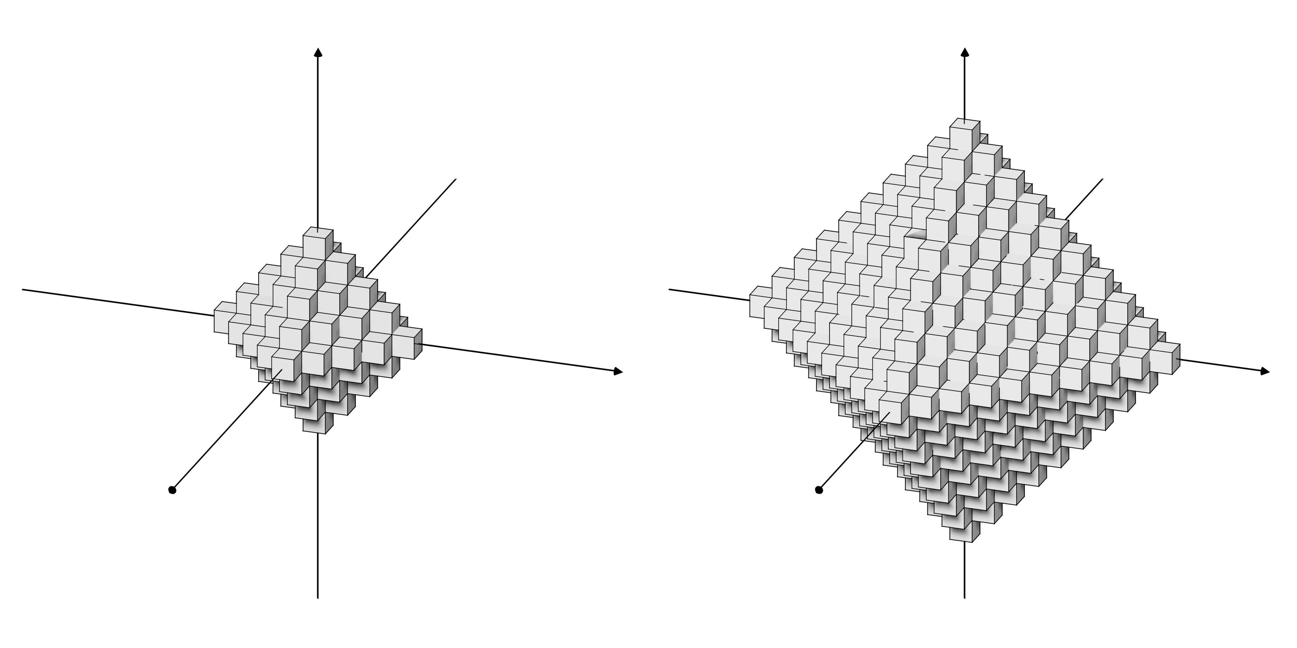
Figure 2: Examples of octahedral surfaces $S_{q}$ used in the ASORA ray-tracing method. All voxels belonging to $S_{q}$, with $q>1$, depend strictly on voxels from the previous shell $S_{q-1}$. Examples $q=4$ (left) and $q=9$ (right) are shown, with the source at the origin of the axes.

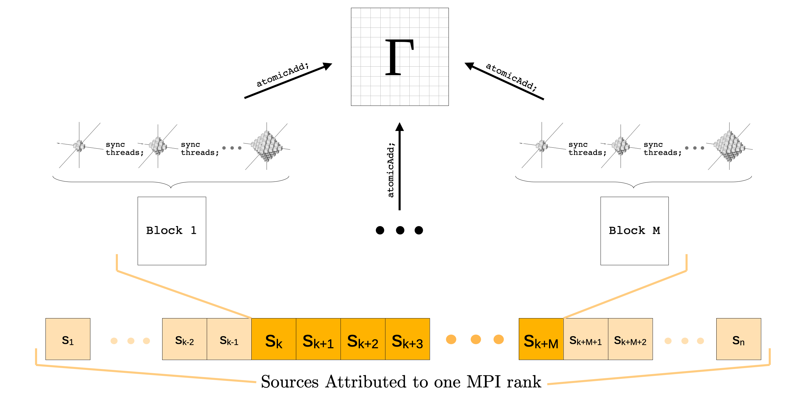
Figure 3: Implementation of the ASORA method. $n$ sources are treated in batches of a given size $M$, and one block is dispatched for each source in the batch. Threads within a block are synchronized between each shell $S_{q}$ but are independent across different sources. Each block atomically adds its contributions to the global ionization rate array. In MPI mode, each rank independently follows the above framework and the $\Gamma$ arrays of all ranks are sum-reduced to the root.

This means that the full ray-tracing work for a single source can be divided into the sequence of tasks $\{S_{q}\}_{q=0}^{Q}$, where $q=0$ corresponds to treating the source voxel itself, and $Q$ is the size of the largest shell. These tasks must be done in order, but within any of them, there are $4q^{2}+2$ operations that can be performed in parallel. Going back to the discussion above, when, for instance, 100 threads are assigned per source for each task with $q\geq 5$, it is theoretically possible for all threads to be actively engaged in performing work. This effectively resolves the challenge of parallelizing the computation on a per-source basis. The full implementation model discussed at the beginning of this section is illustrated in Figure 3.

Furthermore, ASORA is also MPI-enabled, using mpi4py (Dalcin and Fang, 2021) in the same way as it was intended for the original C²-Ray. Namely, the sources are evenly distributed to multiple MPI processes. Each MPI rank maps to one GPU, which then uses the model laid out above to process its subset of sources and broadcasts the result $\Gamma$ to the root rank, using MPI_REDUCE with a sum operation. This allows the use of ASORA on a multi-GPU setup across multiple nodes to further speed up ray-tracing on very heavy workloads.

Finally, rather than giving a maximal shell size $Q$, it is more convenient to set a maximum physical radius $R_{\gamma}$ any photon can travel from the source. If the physical size of a grid voxel is $dr$, the size of the largest shell required to cover the chosen radius fully is given by $Q=\lceil\frac{R_{\gamma}}{dr\sqrt{3}}\rceil$. Any cell inside $S_{Q}$ whose distance to the source exceeds $R_{\gamma}$ can simply be excluded from the computation to yield a spherical region in which $\Gamma$ is nonzero. Further technical details on ASORA can be found in A.

3.4 Python-wrapping of C²-Ray

Here, we provide a brief overview of the pyC²Ray interface and architecture, amalgamating key components from the original Fortran90 code, the new ray-tracing library as discussed below, and elements of pure Python. This integration is facilitated through f2py, a tool developed as part of the NumPy project (Harris et al., 2020). This tool streamlines the creation of extension modules from Fortran90 source files.

The incorporated Fortran90 subroutines primarily encompass the chemistry solver and retain the original CPU-based ray-tracing module as a contingency. The novel ASORA method is written in C++/CUDA and compiled as a Python extension module natively compatible with NumPy. The principal time-evolution function within pyC²Ray is implemented in Python, and it invokes the ray-tracing method, choosing between the CPU and GPU versions and the chemistry method sourced from these extension modules. The prior process of precalculating photoionization rate tables, as introduced earlier, has transitioned to direct implementation in Python. This is achieved using numerical integration techniques from the SciPy library (SciPy 1.0 Contributors, 2020), which relies on the underlying QUADPACK library for lower-level computations. It is worth noting that these integration methods differ from the custom Romberg integration subroutines utilized by the original C²-Ray framework. The commonly needed cosmological equations and physical quantities are now provided by Astropy (Astropy Collaboration, 2022).

Beyond these technical aspects, the inherent method within pyC²Ray—apart from the ray-tracing component—has undergone minimal alteration. Key features of C²-Ray, including photoionization and hydrogen chemistry, have been seamlessly migrated to the Python version without compromising computational efficiency. Our strategy involves a gradual integration of additional extensions over time.

4 Validation Testing & Benchmarking

In § 4.1, we validate our new code using a series of well-established tests, comparing our results to analytical solutions and to the results of our original C²-Ray code. In § 4.2, we investigate how the updated ray-tracing method scales relative to the main problem parameters. In all tests, the temperature conditions of the gas are assumed to be isothermal, i.e. no heating effects are modelled.

4.1 Accuracy Tests

We begin by conducting Tests 1 and 4 from M06, labelled as Test 1 and 2 here, to evaluate the precision of our code in monitoring I-fronts in single-source mode. This evaluation encompasses scenarios both with and without cosmological background expansion. Following this, we investigate the interplay among multiple sources and the occurrence of shadow formation behind an opaque object, Test 3 and Test 4.

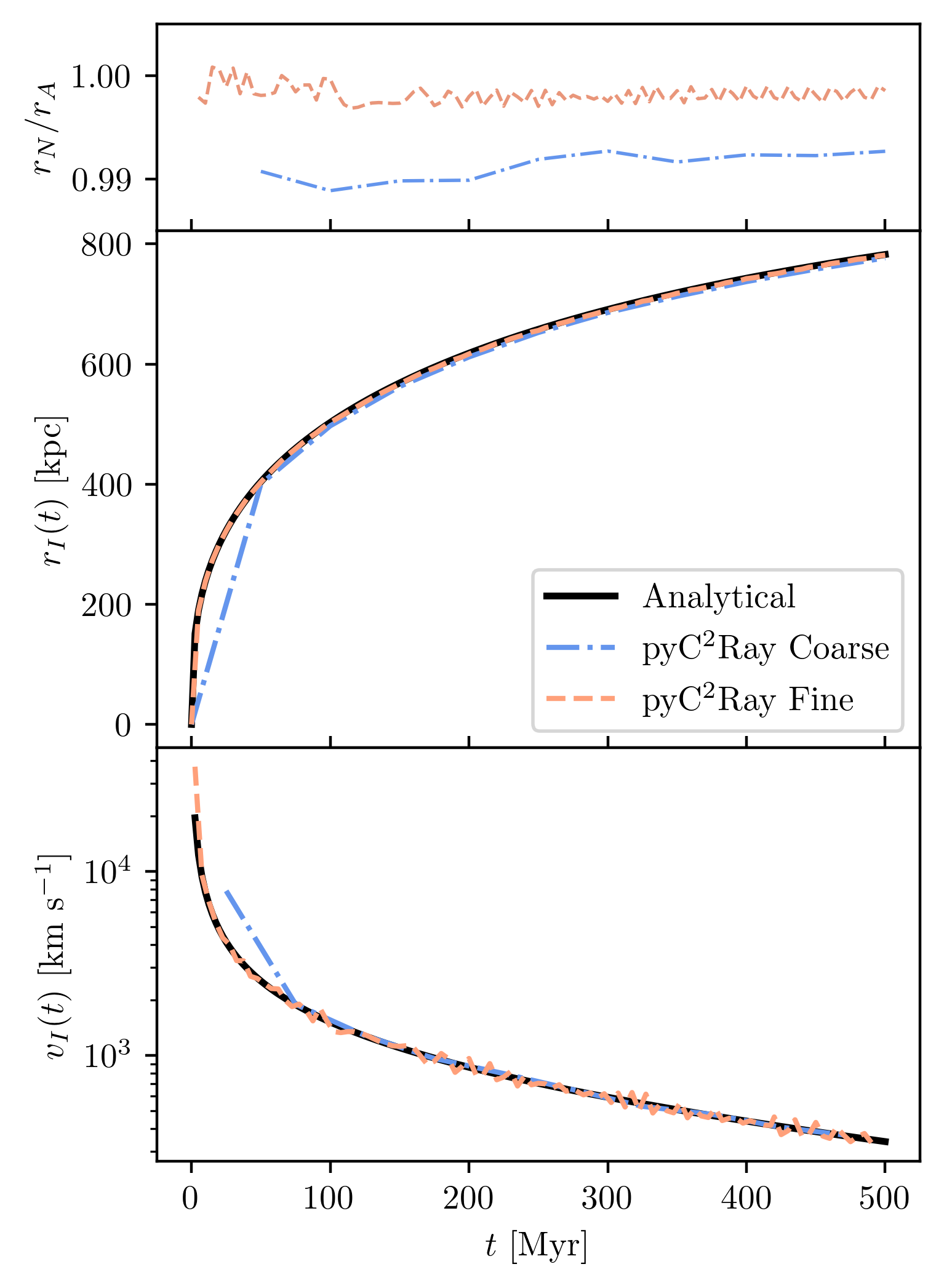
Figure 4: Result for Test 1 (Single-source H II region expansion in uniform gas). The test is conducted with a "coarse" time step $\Delta t_{c}=t_{evo}/10$ and a "fine" one, $\Delta t_{f}=t_{evo}/100$. The time evolution of the ionization front radius (middle) and velocity (bottom) are shown. The error between the numerical and analytical results can be seen in the top panel.

4.1.1 Test 1: Single-Source HII Region Expansion

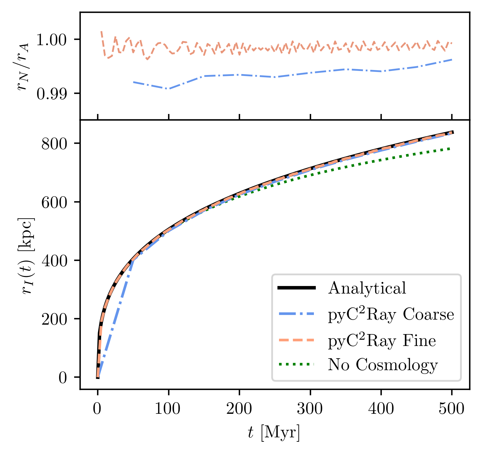
Figure 5: Result for Test 2 (Single-source HII region expansion in cosmological expanding background). Notation is the same as in Figure 4. The source turns on at $z_{i}=9$, and the I-front radius is given in comoving kpc, with the scale factor $a(t_{i})=1$. The green dotted line shows the analytical result without cosmological expansion for reference.

Consider the classical scenario of a single ionizing source within an initially-neutral, uniformly dense field at a constant temperature. In this case, any cosmological effects are disregarded. Assuming the photoionization cross section remains frequency-independent, $\sigma_{\nu}=\sigma_{0}$, known as grey opacity, this system has a well-established analytical solution for the velocity and radius of the ensuing ionization front with respect to time. The solution is given by

$$r_{\mathrm{I}}(t) =r_{\mathrm{S}}\left[1-\exp(-t/t_{\rm rec})\right]^{1/3}$$ (11)

$$v_{\mathrm{I}}(t) =\frac{r_{\mathrm{S}}}{3\,t_{\rm rec}}\frac{\exp(-t/t_{\rm rec})}{\left[1-\exp(-t/t_{\rm rec})\right]^{2/3}}\ .$$ (12)

The above expressions depend on the Strömgren sphere radius $r_{\mathrm{S}}$, recombination time $t_{\mathrm{rec}}$ and total ionizing flux emitted by the source (or the number of photons per unit time). These quantities are defined as,

$$r_{\mathrm{S}}= \left(\frac{3\,\dot{N}_{\gamma}}{4\,\pi\,\alpha_{\mathrm{H}}(T)\,n_{\mathrm{H}}^{2}}\right)^{1/3}\ ,$$ (13)

$$t_{\rm rec}= \frac{1}{\alpha_{\mathrm{H}}(T)\,n_{\rm H}}\ ,$$ (14)

$$\dot{N}_{\gamma}= \int_{\nu_{\rm th}}^{\infty}\frac{L_{\nu}}{h\nu}d\nu\ .$$ (15)

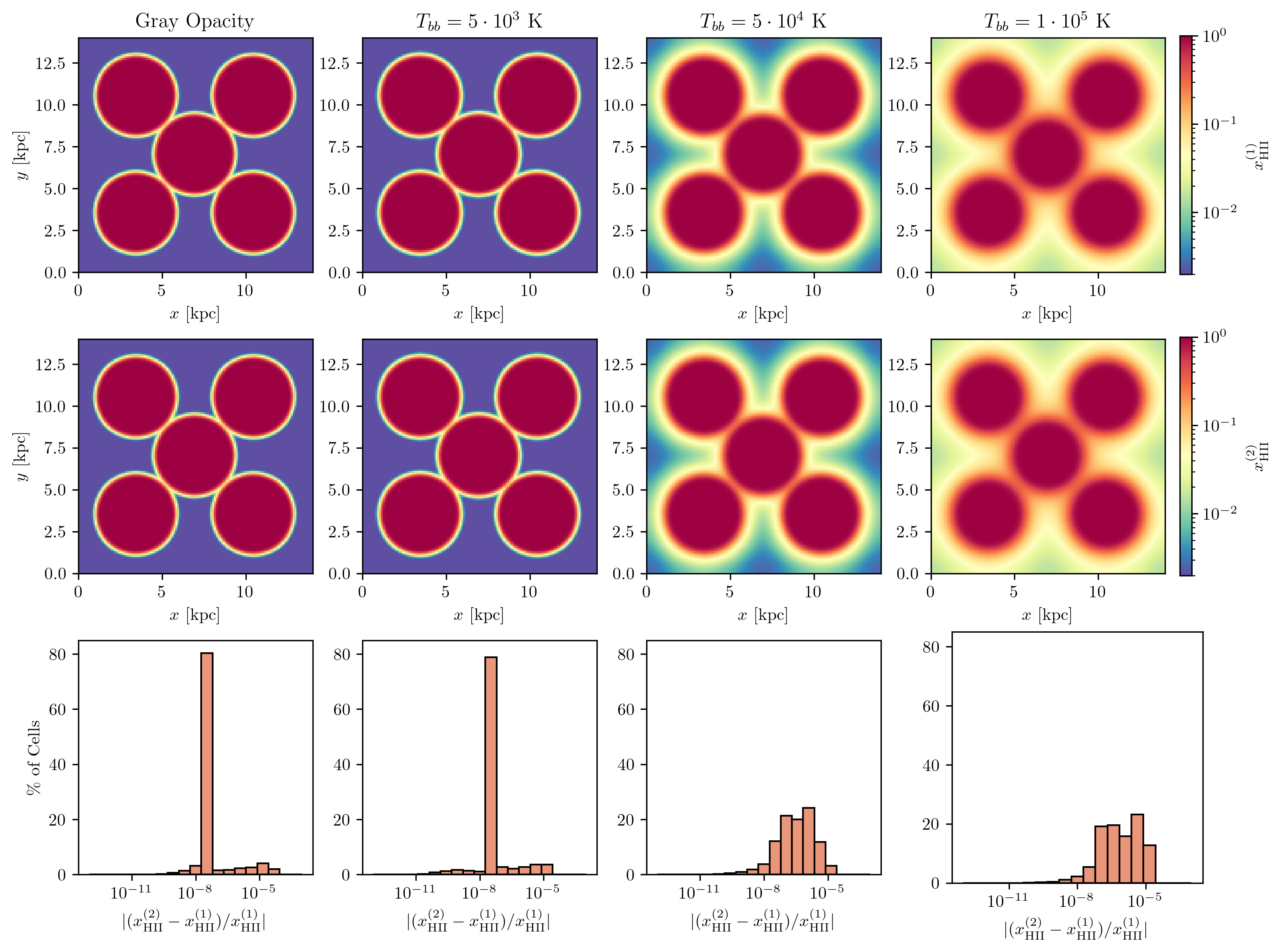
Figure 6: Result for Test 3 (Expansion of Overlapping H II regions around Multiple Black-Body Sources). The top and middle rows show slices through the simulation domain at the $z$-coordinate of the 5 sources, for C²-Ray and pyC²Ray respectively. The leftmost column corresponds to the case with grey opacity, and the remaining 3 columns to those where black body spectra with different temperatures $T_{bb}$ were used. Colours are normalized across each row. The bottom row shows the distribution of relative per-voxel errors between the 2 codes for the whole 3D grid in all 4 cases.

We conduct our first test using the following numerical parameters: the strength of the source is $\dot{N}_{\gamma}=10^{54}$ s^-1, the number density of hydrogen $n_{\mathrm{H}}=1.87\times 10^{-4}$ cm^-3, its temperature $T=10^{4}$ K and the simulation box size is $L=5\times 10^{24}\,{\rm cm}\simeq 1.6\,{\rm Mpc}$. As stated above, we use the case B recombination coefficient for Hydrogen, $\alpha_{\mathrm{H}}(T=10^{4}\,{\rm K})=2.59\times 10^{-13}\,\rm cm^{3}\,s^{-1}$. The simulation is run with mesh size $256^{3}$ for $t_{\rm evo}=500\,\rm Myr$, once with a coarse time step $\Delta_{t}=50\,\rm Myr$ and once with a fine one, $\Delta t=5\,\rm Myr$ (as in M06). We track the position of the I-front along the $x$-axis and define $r_{\mathrm{I}}(t_{k})$ as the radius where $x_{\rm HI}=0.5$. The precise location within a voxel is found by linear interpolation. The numerical I-front velocity, $v_{\mathrm{I}}$, is found by finite-differencing $r_{\mathrm{I}}$, using the same approach as in M06.

The results are shown in Figure 4, where the three panels contain the time evolution of the ratio between numerical to analytical results (top), the I-front radius (middle) and its velocity (bottom). pyC²Ray is in excellent agreement with the analytical prediction, with a coarse and a fine time step choice. In both cases, the $r_{I}$ is slightly underestimated by a constant offset, which can be attributed to the arbitrary choice of $x_{\rm HI}=0.5$ as a definition for $r_{I}$ and the fact that the I-front has a finite thickness (Spitzer, 1998), whereas the analytical solution assumes it to be a sharp transition.

4.1.2 Test 2: Single-Source HII Region in expanding background

We next test if pyC²Ray correctly models the propagation of I-fronts in an expanding universe. Test 2 uses the same source parameters as Test 1, with the source turning on at $z=9$ and then shining for 500 Myr, while the background density starts with the same value as before and evolves with the expansion of the universe. Shapiro and Giroux (1987) showed that a generalized analytical solution exists in this case. The comoving I-front radius is given by $r_{\mathrm{I}}(t)=r_{\mathrm{S},i}\,y(t)^{1/3}$, where $r_{\mathrm{S},i}=(3\dot{N}_{\gamma}/4\pi\alpha_{\mathrm{H}}(T)n_{\mathrm{H},i}^{2})^{1/3}$ is the instantaneous Strömgren radius at the ignition time, $t_{i}$, of the source (with the scale factor set to unity at $t_{i}$, $a_{i}=1$), and

$$y(t)=\lambda e^{\lambda t_{i}/t}\left[\frac{t}{t_{i}}E_{2}(\lambda t_{i}/t)-E_{2}(\lambda)\right],$$ (16)

where $E_{2}(x)=\int_{1}^{\infty}t^{-2}e^{-xt}dt$ is the second-order exponential integral. $\lambda=t_{i}/t_{\mathrm{rec},i}$ is the ratio of the age of the universe at source ignition to the recombination time at that age. We set up the test with $n_{H,i}=1.87\times 10^{-4}\,\mathrm{cm}^{-3}$ and $L_{i}=7\times 10^{24}~{}$cm and using otherwise the same parameters as before. The result is shown in Figure 5, where $r_{I}(t)$ represents the comoving I-front radius, keeping in mind that $a(t_{i})=1$. For this test, we used the same cosmology as in M06, namely $h=0.7$, $\Omega_{M}=0.27$ and $\Omega_{b}=0.043$.

pyC²Ray again shows excellent agreement with the analytical result. While the effect of cosmic expansion is not evident at first sight, the analytical prediction without cosmology, Equation 11, is also plotted for reference in the figure (green dotted line), and the difference is clearly visible. Again, results are almost as accurate when using a coarse time step.

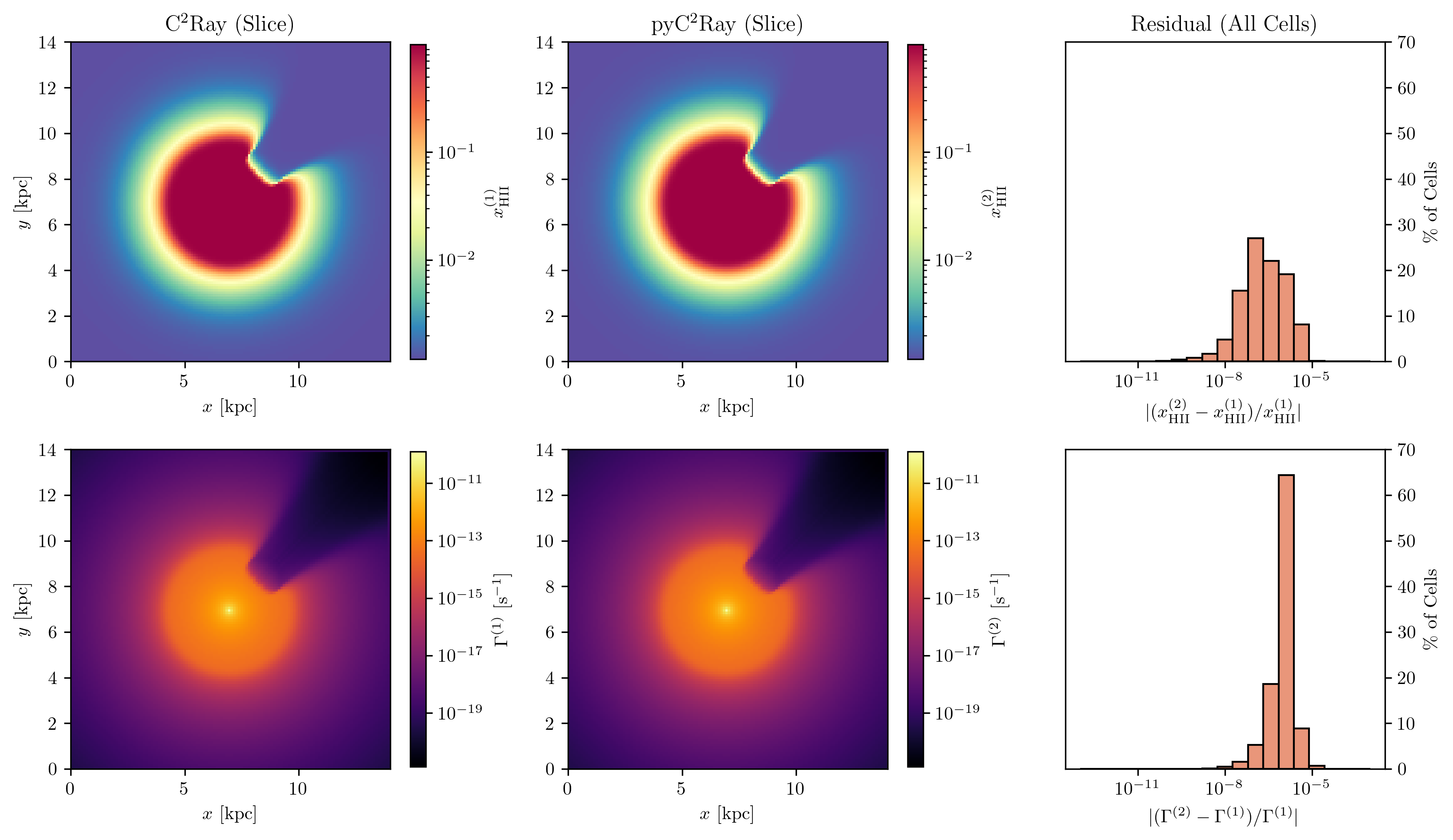
Figure 7: Result for Test 4 (I-Front Trapping in a Dense Clump and Formation of a Shadow). Shown are slices through the $z$-plane containing one ionizing source at the centre and a dense clump of hydrogen diagonally offset from the source. The top row shows the ionized hydrogen fraction for C²-Ray (left) and pyC²Ray (middle), as well as the relative error between the two (right). The bottom row shows the same comparison for the photoionization rate.

4.1.3 Test 3: Expansion of Overlapping HII regions around Multiple Black-Body Sources

Now we turn to the more realistic case of non-grey opacity and parameterize the cross section as $\sigma_{\nu}=\sigma_{0}(\nu/\nu_{0})^{-\alpha}$, where $\nu_{0}$ is the ionization threshold frequency. The parameters of the power law are as in M06, $\sigma_{0}=6.3\times 10^{18}$ cm^-2 and $\alpha=2.8$. We test how the aspect of the ionization front is affected by the spectral characteristics of the sources. For harder spectra, where the energy peak is well above the ionization threshold, we expect wider ionization fronts, as the hard photons can penetrate deeper into the medium (Spitzer, 1998). To test this and at the same time visualize how different HII regions overlap, we place 5 black-body sources, each with total ionizing flux $\dot{N}_{\gamma}=5\times 10^{48}$ but with different temperatures $T_{bb}$, in a dice-like pattern on the same $z$-plane. The box size is $L=14$ kpc, the mesh $128^{3}$ and the constant hydrogen density is $n_{H}=10^{-3}$ cm^-3. We simulate for $t_{evo}=10\,\rm Myr$, with time step $\Delta t=1\,\rm Myr$. Figure 6 shows cuts through the source plane of the final ionized hydrogen fraction $x_{\rm HII}$, for pyC²Ray (top) and C²-Ray(middle), along with the distribution of the absolute relative error, $\left|(x_{\rm HII}^{\text{{pyC${}^{2}$Ray}{}}}-x_{\rm HII}^{\text{{C${}^{2}$-Ray}{}}})/x_{\rm HII}^{\text{{C${}^{2}$-Ray}{}}}\right|$, between the two coeval cubes (bottom panels). The leftmost column is the grey-opacity case as in the two previous tests, while the three remaining columns contain the results for $T_{bb}=\{5\times 10^{3},5\times 10^{4},1\times 10^{5}\}\,\rm K$.

Qualitatively, both C²-Ray and pyC²Ray reproduce the expected softness of ionization fronts for hot spectra, and the overlap of individual H II regions is also correctly modelled. The largest value for the relative error is on the order $10^{-4}$ in all cases, while the mean increases for harder spectra. Although relatively small, this error requires an explanation, as both codes should, in principle, produce equal results in the absence of unit conversion or floating point errors. In fact, an important technical difference between the two, namely the choice of numerical integration method used to pre-compute Equation 6, which was mentioned in the introduction, is the most likely explanation for this result. Indeed, C²-Ray uses a custom-written set of subroutines implementing the Romberg method, while in pyC²Ray, we use the standard quad wrapper of SciPy, which uses the adaptive quadrature method, the QUADPACK library. Both methods are valid choices, but they will inevitably yield slightly different results depending on the chosen resolution. We tested this by varying the frequency bins used by the Romberg method in C²-Ray and found that the relative error between the two codes drops significantly as this number increases.

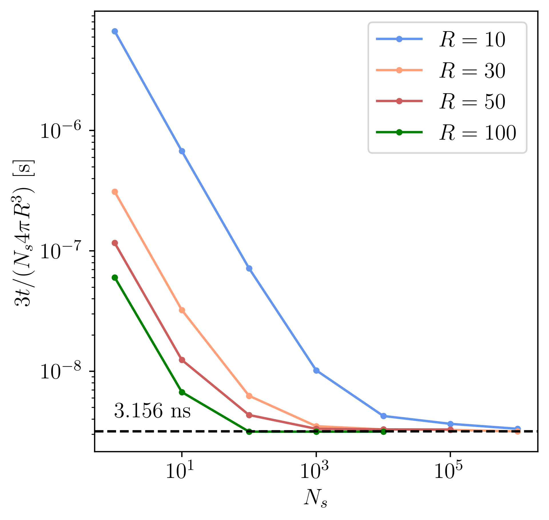
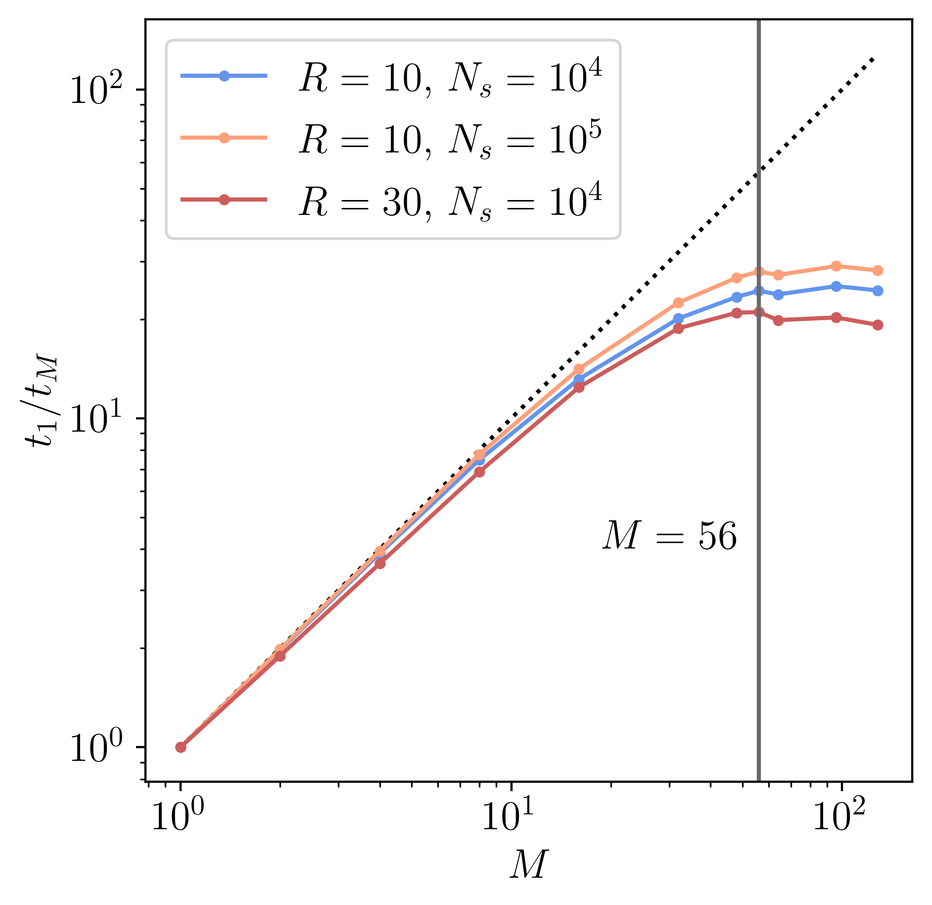
Figure 8: Scaling of the ASORA ray-tracing library. Left: Computation time per source per voxel for an increasing number of sources $N_{s}$ and different ray-tracing radii $R$. This time approaches a constant value as more sources are added and faster for larger $R$. Right: Speedup in terms of the number of blocks $M$, given by $t_{1}/t_{M}$, where $t_{1}$ is the timing when a single block is used. The vertical black line marks $M=56$, corresponding to the number of SMs on the NVIDIA® P100 GPU used in this benchmark.

4.1.4 Test 4: I-Front Trapping in a Dense Clump and Formation of a Shadow

Finally, to probe more specifically the ray-tracing method, we test for the formation of a shadow behind an overdense region. Correct modelling of shadows is one of the key advantages of ray-tracing over other techniques, making this an important check. In this test, the box size is $L=14$ kpc with mesh $128^{3}$ and a source with total ionizing flux $\dot{N}_{\gamma}=10^{49}$ s^-1 is placed at its centre. The hydrogen has a mean density $\bar{n}_{\rm H}=10^{-3}$ cm^-3, and a spherical overdense region of radius $r=8.75$ pc is placed on the same $z$-plane as the source, at a distance $d=2.01$ kpc diagonally from it. Within this region the density is $n_{\mathrm{H}}^{\star}=6\,\bar{n}_{\rm H}$. The source has a black body temperature $T_{bb}=5\times 10^{4}$ K, and $t_{\rm evo}$ and $\Delta_{t}$ are as in Test 3. The result is visualized in Figure 7, where a cut through the source plane of the final ionized hydrogen fraction $x_{\rm HII}$ is shown on top and the photoionization rate $\Gamma$ below, for both codes along with the relative error as before. We want to point out that the fuzziness of the shadow is a feature of the short characteristic ray-tracing. The relative error is again small, and we believe it to be due to the choice of integration method as in the previous test. Interestingly, this error is larger by an order of magnitude at the edge of the overdense region. This is not so surprising, given that the overdensity is very optically thick and thus contains a large density gradient at its boundary. We noticed that the relative error is negative closer to the source, then positive and then close to 0, reflecting the net photon flux conservation.

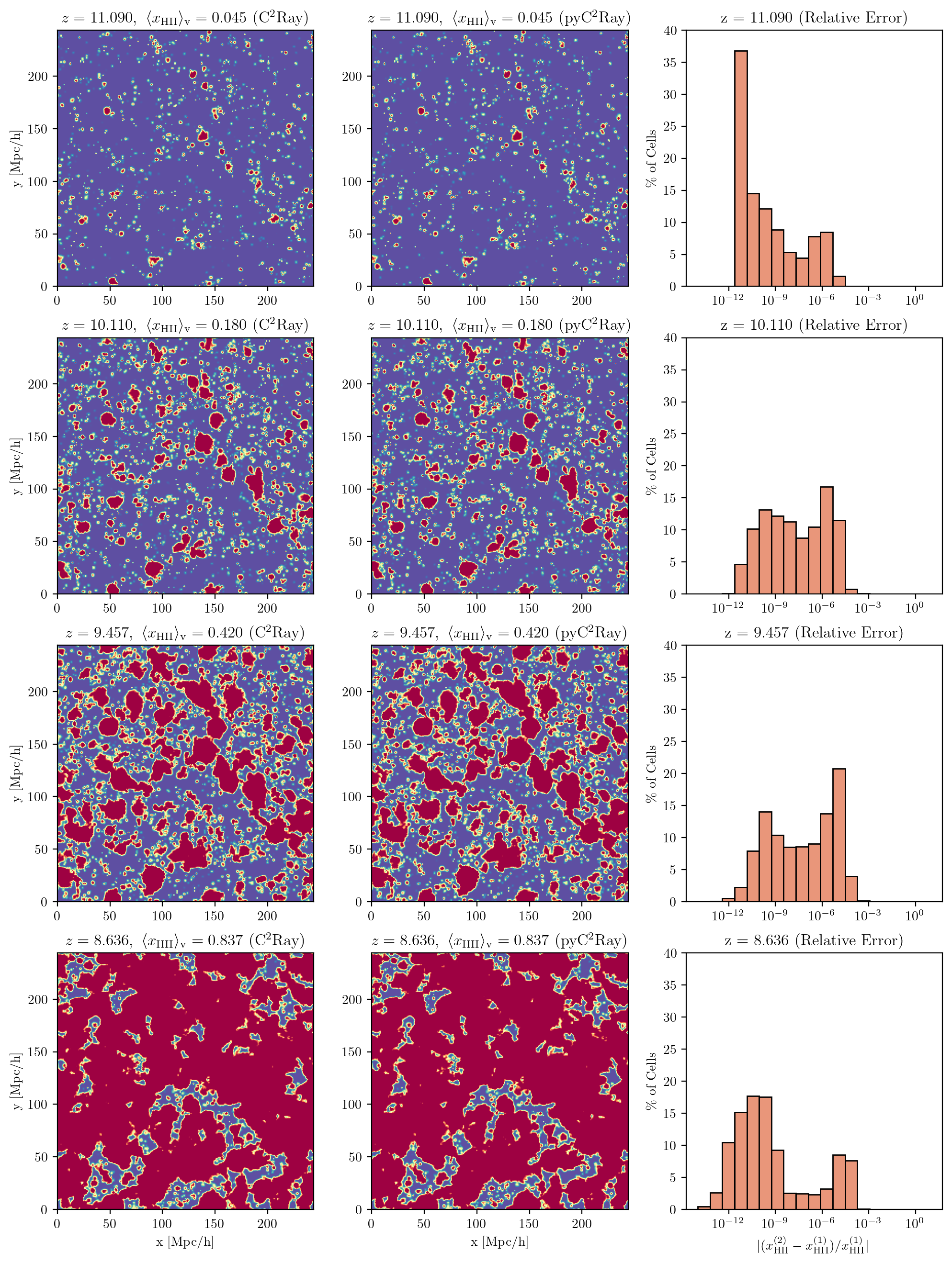
Figure 9: Results from of the $349\,\rm cMpc$ EoR test simulation. The left and middle columns show slices through the simulation domain for C²-Ray and pyC²Ray, respectively. The right column shows the distribution relative per-voxel error for the 250³ grid. The simulation includes only dark matter halos masses with an efficiency factor $f_{\gamma}=30$ and a maximal comoving photon radius $R=15\,\rm cMpc$.

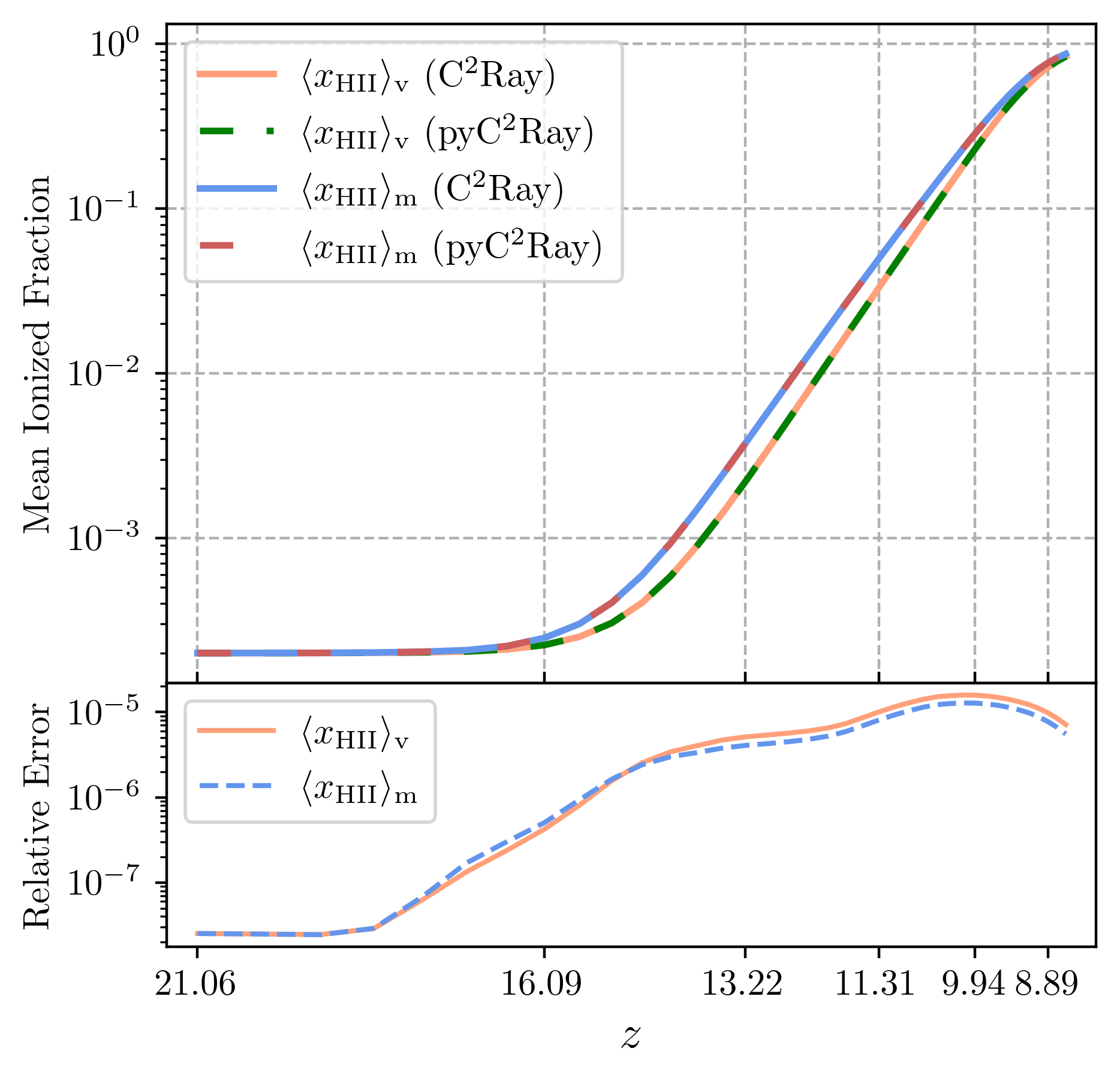
Figure 10: Left: Comparison of reionization history from the 349 Mpc EoR test simulation, performed with C²-Ray and pyC²Ray. The top panel shows the evolution of the volume $\langle x^{\mathrm{v}}_{\mathrm{HII}}\rangle$ and mass-averaged $\langle x^{\mathrm{m}}_{\mathrm{HII}}\rangle$ fraction of ionized hydrogen over the redshift range $z\in[21.06,8.636]$ and the bottom panel the relative error between the two codes. Right: Comparison of the 21-cm power spectra from the same simulation at different redshifts (indicated in the legend) reveals a consistent match between C²-Ray and pyC²Ray.

4.2 Performance Benchmark

We now examine more closely the performance of the new ray-tracing library. All benchmarks in this section are performed on a size $N=250$ grid and run on one node of the Piz Daint computer at CSCS, containing in particular a single NVIDIA®  Tesla P100 GPU. First, we determine how the ray-tracing performance scales as more sources are added, or the radius of ray-tracing per source increases. We expect the code to scale linearly with the number of sources $N_{s}$ and as $\mathcal{O}(R^{3})$ with the ray-tracing radius, $R=N_{mesh}\cdot R_{\rm max}/L_{\rm B}$, where $R_{\rm max}$ is the maximum radius for ray-tracing and $L_{\rm B}$ the box size, both in $\rm cMpc$ units. The benchmark is set up as follows. For $R=[10,30,50,100]$, the ray-tracing routine is called (on its own, without solving the chemistry afterwards) on $N_{s}=10^{a},\ a=0,\dots,6$ sources and its run time is averaged over 10 executions. The left panel of Figure 8 shows the computation time per source per voxel,

$$\Delta t(N_{s},R)=\frac{t(N_{s},R)}{\frac{4}{3}\pi R^{3}N_{s}},$$ (17)

where $t(N_{s},R)$ is the run time of the function running on $N_{s}$ sources and computing $\Gamma$ in a spherical volume of radius $R$ (in voxel units) for each of them. With increasing $N_{s}$, $\Delta t(N_{s},R)$ approaches a constant value of about $3.156\,\rm ns$ on our system. Furthermore, this convergence is faster when the radius $R$ is larger. This implies that when few sources are present, overheads represent a non-negligible fraction of the execution time, even more so when the work per source (determined by $R$) is low. However, we can see that above $\sim 1000$ sources, the execution time is very close to its minimum, even for a relatively small RT radius. When there are few sources, the total amount of work is low and is not an expensive calculation. But typically, EoR simulations require $N_{s}\gg 1000$. Our code runs in a regime where the work and not overheads dominate the performance of the code.

Next, we test how the code scales as the source batch size $M$ increases, corresponding to increasing the number of CUDA blocks dispatched to the device between global synchronizations. The right panel of Figure 8 presents the speedup $t_{1}/t_{M}$ (where $t_{M}$ is the execution time using $M$ blocks) achieved in 3 cases; $(R=10,N_{s}=10^{4})$, $(R=10,N_{s}=10^{5})$ and $(R=30,N_{s}=10^{4})$ to see the impact of both the radius and total number of sources. This test is an analogue of the "strong scaling" measurement typically performed on CPU cores. We observe that on our system, in all 3 cases, the code scales well up to $M\sim 32$ and does not gain any performance above $M\sim 50$. These results indicate that the amount of resources required by each block is quite high and that some limit of the GPU is reached before the number of blocks is as large as the number of SMs on the device (56 for the P100 used here). Further profiling has revealed that the number of registers per thread required by the ray-tracing kernel prevents the code from reaching 100$\%$ occupancy in its current state, even on GPUs with higher compute capability than the P100. Overcoming this limitation should be one of the main targets for future performance updates.

Two conclusions arise from this section: (1) The library is most optimized for use cases where many sources are present in the simulation, as is the case in EoR modelling. However, in cases where few sources are present, it will run optimally if the number of raytraced voxels is large. This may be the case when performing high-resolution radiative transfer simulations of smaller volumes, thus expanding the possible usage scenarios for pyC²Ray. (2) A good value for the batch size $M$ will depend strongly on the system on which the code is run while simultaneously being limited by the available memory. This is because each block needs a cache space for the ray-tracing, the size of which scales with the grid, i.e. $\mathcal{O}(N^{3})$.

5 Running a Cosmological Reionization Simulation

The ultimate test for the updated code is to see whether it can reproduce the results of a simulation performed with the original C²-Ray while at the same time achieving a gain in performance. Here, we post-process a $(349\mathrm{Mpc})^{3}$ volume $N$-body simulation run with $4000^{3}$ dark matter particles, which models the formation of high-redshift structures. These $N$-body simulations used the code CUBEP³M (Harnois-Déraps et al., 2013), which has an on-the-fly halo finder, providing halo catalogues at each redshift snapshot using the spherical overdensity method (see Watson et al., 2013, for more detail). The $N$-body dark matter particles and the halo catalogue are then gridded, with an SPH-like smoothing technique, onto a regular grid of size $N_{\rm mesh}=250^{3}$ that is later used as inputs for the RT simulation. This simulation resolves dark matter haloes with mass $M_{\rm halo}\geq 10^{9}{\rm M_{\odot}}$. This simulation contains approximately $10^{7}$ sources toward the end of reionization. See Dixon et al. (2016) and Giri et al. (2018) for more detailed descriptions.

We follow the same source model presented in previous work (e.g. Iliev et al., 2014; Bianco et al., 2021) that assumes a linear relation between the emissivity and the mass of the hosting dark matter halo. In this model, the grand total of ionizing photons, $\dot{N}_{\gamma}$, produced by a source residing in dark matter halo mass $M_{\rm halo}$ is

$$\dot{N}_{\gamma}=f_{\gamma}\,\frac{M_{\rm halo}\,\Omega_{\rm b}}{\Omega_{\rm M}\,m_{p}\,t_{s}},$$ (18)

where the efficiency factor $f_{\rm\gamma}=30$ and the source lifetime $t_{s}\approx 10\,{\rm Myr}$ is taken to be the time difference between the simulation snapshots. Two-time steps are performed for each redshift interval. Here, we choose an extreme value for the efficiency factor to speed up the reionization process so we could run C²-Ray in a reasonable amount of time and computational resources. We should note that reionization ends quite early compared to more realistic models in Dixon et al. (2016) and Giri et al. (2019) produced using C²-Ray—however, the outcomes of the comparison hold for any source model.

In Figure 9, we show slices of the simulated ionized fraction, $x_{\rm HII}$, comparing C²-Ray (left column) and pyC²Ray (middle column) at redshift $z=11.090,\,10.110,\,9.457$ and $8.636$, corresponding to a volume-averaged ionized fraction $\left<x_{\rm HII}\right>=0.045,\,0.180,\,0.420$ and $0.837$. We show the relative error in the right column of the same figure for each redshift. At high redshift, the error distribution is mostly centred at $10^{-6}$, similar to what we show in § 4.1.3 and 4.1.4. While from $z\sim 10$, it shows two peaks with the distribution transitioning from $10^{-4.5}$ to $10^{-10}$. The double-peaked feature of the error distribution is visible from the moment the source contribution becomes substantial. This indicates that the error distribution is at first associated with the precision error in the vast neutral field while later with the growing ionized regions. In the left panels of Figure 10, we calculate the volume- and mass-averaged ionized fraction, $\left<x_{\rm HII}\right>_{\rm v}$ and $\left<x_{\rm HII}\right>_{\rm m}$, against redshift. With solid lines, we indicate the results obtained with C²-Ray, while in dashed lines, the one with pyC²Ray. Similar to what we show in the previous paragraph, on average, the relative error is at least five orders of magnitude smaller, $\sim 10^{-5}$, compared to the dynamic range of the ionized field, making the difference indiscernible. Notice that we show the result to $z=8.575$ when the IGM is about $86\%$ ionized. However, at this reionization epoch, the simulation has approximately $\sim 1.5\times 10^{6}$ sources, and C²-Ray starts to become computationally demanding.

Radio experiments, such as HERA, LOFAR, and MWA, aim to observe the spatial distribution $\boldsymbol{r}$ of the differential brightness temperature $\delta T_{\mathrm{b}}(\boldsymbol{r},z)$ corresponding to the 21-cm signal. This quantity can be given as (e.g. Pritchard and Loeb, 2012),

$$\delta T_{b}(\boldsymbol{r},z)\approx 27~{}\mathrm{mK} \left(\frac{0.15}{\Omega_{M}h^{2}}\frac{1+z}{10}\right)^{\frac{1}{2}}\left(\frac{\Omega_{b}h^{2}}{0.023}\right)$$ (19)

$$\times[1-x_{\rm HII}(\boldsymbol{r},z)][1+\delta_{\rm b}(\boldsymbol{r},z)],$$

where $x_{\mathrm{HII}}$ and $\delta_{\mathrm{b}}$ are ionization hydrogen fraction and baryon overdensity, respectively. We should note that we have assumed a spin temperature to be saturated and ignore the impact of redshift-space distortion. We refer the interested readers to Ross et al. (2021) for exploration of both these aspects in simulations with C²-Ray. We compute $\delta T_{\mathrm{b}}(\boldsymbol{r},z)$ and subsequently the power spectrum using reionization simulation snapshots with our data analysis software, Tools21cm (Giri et al., 2020). In the top-right panel of Figure 10, we present the 21-cm power spectrum at various redshifts. We observe a precise agreement between the results obtained from pyC²Ray and C²-Ray, also evident from the relative error in the bottom-right panel, demonstrating that these upgrades can accurately replicate the spatial distribution of the 21-cm signal.

The simulation with pyC²Ray cost $2.5$ GPU-hours on our single-GPU system, while the comparison run, with the Fortran90 CPU version of C²-Ray, computed on 128 cores for a total of $13,824$ core-hours. While GPU-hours are, in general, more expensive than core-hours, the observed speedup is so large that pyC²Ray is significantly cheaper to run than the original code by a factor of $\sim 100$, depending on the computing centre, which was part of the motivation behind this update.

6 Summary and Conclusions

The main challenge in simulating the cosmic Epoch of Reionization is that we are required to concurrently simulate a large volume of the order of the $\rm Gpc$ scale while resolving compact and dense cosmic structures. These requirements make Radiative Transfer (RT) simulations extremely computationally expensive and demanding. For this reason, the majority of RT codes are implemented with computing languages suited for scientific computing, such as Fortran90 or C/C++. However, this makes any changes or regular updates to the code cumbersome for new users, as any slight modification requires frequent recompilation and debugging. Moreover, relatively little effort has been made to make RT simulation computationally efficient and functional on general-purpose graphic process units (GPU).

Therefore, this paper introduces pyC²Ray, a Python wrapped updated version of the extensively used C²-Ray RT code for cosmic reionization simulations. In particular, we present the newly developed Accelerated Short-characteristics Octhaedral RAy-tracing algorithm, ASORA, that utilizes GPU architectures achieve drastic speedup in fully numerical RT simulations.

In § 2, we recap the differential equation solved during a cosmological reionization simulation. In § 2.1, we summarize the well-established time-averaged method that solves the chemistry equation in C²-Ray, Equation 1, allowing the solution to be integrated on a larger time-step compared to the reionization time scales, otherwise required by a more direct approach. In § 2.2, we explain in detail the necessity for an efficient ray-tracing method for our code. With Equation 5 and 7, we highlight the core and most computationally expensive operation in RT algorithms, which consists of computing the column density and, thus, the optical depth for each voxel, that ultimately quantifies the number of ionizing photons that are absorbed by a cell along the ray. The combination of the time-averaged and short-characteristics methods are the distinguishing features of the C²-Ray code. In Figure 1, we summarize the algorithm for both the C²-Ray and pyC²Ray methods presented here.

In § 3.1, we remind the reader of the short-characteristic approach of C²-Ray inherited by pyC²Ray. In § 3.2, we describe the existing CPU parallelization of the current version of C²-Ray, which consists of splitting the source input list into equal parts for each MPI processor. For each rank, 8 OpenMP threads, corresponding to the number of independent domains around each source, compute the $\rm HI$ column density. This parallelization strategy is not optimal for GPU architectures. Therefore, in § 3.3 we propose a new interpolation approach for the C²-Ray RT algorithm specifically designed for GPUs. The ASORA interpolation scheme comes from the physical intuition that the radiation propagates as an outward wavefront around a source. This new approach changes the domain decomposition to an interpolation between concentric surfaces of an octahedron, centred around the source as illustrated by Figure 2. From a technical perspective, in pyC²Ray, we keep the same MPI source distribution, as presented in § 3.2, and instead replace the OpenMP domain decomposition with the ASORA method.

The update also includes the conversion to Python of the non-time-consuming subroutines of C²-Ray. In § 3.4, we mention how the use of commonly used libraries, such as Numpy, Scipy and Astropy can be easily included according to the user’s need. Moreover, the pyC²Ray user interface makes it easier to employ other codes that have also been Python-wrapped. For instance, we can easily incorporate in pyC²Ray photo-ionization rates from other spectral energy distributions calculated with a population synthesis code such as PEGASE-2 (Fioc et al., 2011) or a different chemistry solver such GRACKLE (Smith et al., 2017).

In § 4, we show pyC²Ray results on a series of standard RT tests. In § 4.1.1 and 4.1.2, we demonstrate that pyC²Ray agrees with the analytical solutions of the ionization front size, $r_{\rm I}$, for the single sources in a static and expanding lattice. To test that the conversion to Pyhton of the non-time-critical subroutines was successful and does not introduce substantial differences, in § 4.1.3, we test the results on overlapping $\rm HII$ regions for sources with different black body spectra. In § 4.1.4, we probe the formation of a shadow behind an overdense region, a standard test for ray tracing methods.

In § 4.2, we examine the performance of the new ray-tracing methods accomplished on the Piz Daint cluster at the Swiss National Supercomputing Centre (CSCS) equipped with an NVIDIA®  Tesla P100 GPU. Our main finding is that the ASORA RT computing time grows linearly with the increasing number of sources, $N_{s}$, and in cubic fashion with respect to the maximum radius for ray tracing, so $R^{3}$, i.e. distance given in number of voxels. In the case of the Tesla P100 GPU, the computing time per source per voxel within the ray-tracing distance saturates with value $3.156\,\rm ns$ when $N_{s}>10^{5}$. This study allows the user to quantify the computing time and cost of a future simulation run with pyC²Ray. If we consider a cosmological simulation with 68 redshift steps, each with 2-time steps, ray-tracing radii $R=11$ and approximately $N_{s}\approx 4\times 10^{6}$ sources, we can run the entire simulation from $z=21$ to $8.5$ with a total of $\sim 2.75$ GPU-h, which corresponds to the cost obtained in the cosmological example presented in §5. Secondly, the method scales strongly with the batch size up to $\sim 32$ on our system, suggesting that the GPU occupancy is not yet optimal, an issue which may be addressed in future updates. We estimate that running a reionization simulation on the same volume down to $z\sim 6$, where $N_{s}=1.5\times 10^{7}$, would cost approximately 10.3 GPU-h.

Finally, in § 5, we compare pyC²Ray and C²-Ray on an actual cosmological simulation. We demonstrate that the differences within the same simulation are negligible with an absolute-relative error between $10^{-4}$ and $10^{-12}$ on the $\rm HII$ field, while both mass- and volume-averaged ionized fractions and the power spectra accumulate an error that stays below the order of $<10^{-5}$. As mentioned in the previous paragraph, the computational cost for this simulation was $2.5$ GPU-hours, while the same simulation run on $128$ cores with C²-Ray took $\sim 14\rm k$ core-hours. Another way to describe the gain in performance is to consider the monetary cost of running these simulations. The cost of running a code on a GPU or CPU cluster varies based on the electricity consumption and other indirect expenses assessed by the high-performance computer facility. Nowadays, one GPU-hour can cost on average $0.8\,\rm Euros$, while one core-hour can be $0.01\,\rm Euros$. Therefore, with these reference fees the simulation presented § 5 would have cost $2\,\rm Euros$ if run with pyC²Ray instead of $138.25\,\rm Euros$ with C²-Ray.

With this work, we demonstrate that pyC²Ray achieves the same result as C²-Ray for a cosmological EoR simulation, but with a computing cost and time two orders of magnitude faster than the original code, confirming the motivation behind this modernization of C²-Ray. In this update, we focused on the most simple simulation setup, namely, no photo-heating and only photo-ionization for hydrogen chemistry. As mentioned, C²-Ray has been extended to also include helium (Friedrich et al., 2012) and X-ray heating (Ross et al., 2017), and has also been used as a module in a hydrodynamic simulation to follow the evolution of an HII region in the interstellar medium (ISM), see Arthur et al. (2011) and Medina et al. (2014). We aim to gradually include these features and extensions in pyC²Ray now that the groundwork has been laid.

Appendix A ASORA Implementation Details

Here, we briefly discuss how the ASORA method is implemented in C++/CUDA. As detailed in the paper, each block is assigned to a single source and owns a dedicated memory space to store the values of the column densities of voxels to be used as interpolants in upcoming tasks. Each task $S_{q}$ comprises the $|S_{q}|=4q^{2}+2$ grid voxels belonging to an octahedral shell as illustrated in Figure 2. Threads within a block are labelled by 1D indices $x=0,\dots,N$, where $N$ is the block size. Labelling the voxels in the shell by $s=0,\dots,|S_{q}|$, all voxels can be treated if the threads iterate $\sim|S_{q}|/N$ times. It then remains to map the 1D indices $s$ to the actual 3D grid positions $(i,j,k)$ of the voxels within the shell. We use the following mapping: separate the octahedron into a "top" part containing all $k\geq k_{s}$ planes, where $k_{s}$ is the source plane, and a "bottom" part containing the rest. For the top part, which contains $2q(q+1)+1$ voxels in total, the $k$ index of any voxel can be found from its $i,j$ indices through $k=k_{s}+q-(|i-i_{s}|+|j-j_{s}|)$. To find $i,j$, we follow the procedure illustrated in Figure 11: map $s=1,\dots,2q(q+1)$ to Cartesian 2D coordinates $(a,b)$ as in (A) and apply a shear matrix $(a,b)\rightarrow(a^{\prime},b^{\prime})$ to obtain (B). Apply a translation on the subset of those with $a+2b>2q$ (C) and finally map the remaining voxel $s=0$ to $(i,j)=(i_{s}+q,j_{s})$ to obtain the full squashed top part of the octahedron (D). The same procedure is applied to the lower part, with some slight modifications, as this does not include the source plane, and so contains fewer voxels in total ($2q^{2}-1$). For further details, we refer the reader to the source code.

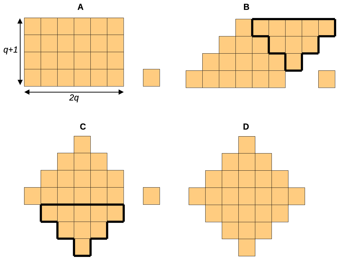
Figure 11: Schematic representation of the mapping of 1D indices $0,\dots,2q(q+1)$ to the 3D grid positions $(i,j,k)$ of voxels in the top part of the $q=3$ shell. The $(i,j)$ mapping is a combination of a shear (B) and a translation (C), and the $k$ coordinate is determined directly from $(i,j)$ as described in the text.

A last key point to address is that since C²-Ray uses periodic boundary conditions, it is important to impose a further constraint on the indices $(i,j,k)$ of the voxels that are allowed to avoid race conditions on coordinates that map to the same voxel under periodicity. The simulation domain is cubic, so this constraint is satisfied if we impose that no voxel can be farther away from the source than the edges of the grid, translated under periodicity. On an odd mesh ($N$ odd), this means only considering voxels at most a grid distance $N/2$ away from the source on either side. On an even mesh, a convention must be chosen, and in line with the original C²-Ray code, we impose that the maximum distance in each dimension is $N/2$ on the negative and $N/2-1$ on the positive side of the source.

References

- Abel et al. (1999) Abel, T., Norman, M.L., Madau, P., 1999. Photon-conserving radiative transfer around point sources in multidimensional numerical cosmology. A&A 523, 66–71. URL: https://doi.org/10.1086/307739, doi:10.1086/307739.
- Arthur et al. (2011) Arthur, S.J., Henney, W.J., Mellema, G., de Colle, F., Vázquez-Semadeni, E., 2011. Radiation-magnetohydrodynamic simulations of H II regions and their associated PDRs in turbulent molecular clouds. MNRAS 414, 1747–1768. doi:10.1111/j.1365-2966.2011.18507.x, arXiv:1101.5510.
- Astropy Collaboration (2022) Astropy Collaboration, 2022. The Astropy Project: Sustaining and Growing a Community-oriented Open-source Project and the Latest Major Release (v5.0) of the Core Package. ApJ 935, 167. doi:10.3847/1538-4357/ac7c74, arXiv:2206.14220.
- Aubert and Teyssier (2008) Aubert, D., Teyssier, R., 2008. A radiative transfer scheme for cosmological reionization based on a local eddington tensor. MNRAS 387, 295–307.
- Barkana (2016) Barkana, R., 2016. The rise of the first stars: Supersonic streaming, radiative feedback, and 21-cm cosmology. Physics Reports 645, 1–59.
- Bianco et al. (2021) Bianco, M., Iliev, I.T., Ahn, K., Giri, S.K., Mao, Y., Park, H., Shapiro, P.R., 2021. The impact of inhomogeneous subgrid clumping on cosmic reionization – II. Modelling stochasticity. MNRAS 504, 2443–2460. URL: https://doi.org/10.1093/mnras/stab787, doi:10.1093/mnras/stab787.
- Bosman et al. (2022) Bosman, S.E., Davies, F.B., Becker, G.D., Keating, L.C., Davies, R.L., Zhu, Y., Eilers, A.C., D’Odorico, V., Bian, F., Bischetti, M., et al., 2022. Hydrogen reionization ends by z= 5.3: Lyman- optical depth measured by the xqr-30 sample. MNRAS 514, 55–76.
- Cavelan et al. (2020) Cavelan, A., Cabezón, R.M., Grabarczyk, M., Ciorba, F.M., 2020. A Smoothed Particle Hydrodynamics Mini-App for Exascale, in: PASC ’20: Proceedings of the Platform for Advanced Scientific Computing ConferenceJune 2020, p. 11. doi:10.1145/3394277.3401855, arXiv:2005.02656.
- Choudhury (2009) Choudhury, T.R., 2009. Analytical models of the intergalactic medium and reionization. arXiv:0904.4596.
- Choudhury and Ferrara (2006) Choudhury, T.R., Ferrara, A., 2006. Physics of cosmic reionization. arXiv:astro-ph/0603149.
- Dalcin and Fang (2021) Dalcin, L., Fang, Y.L.L., 2021. mpi4py: Status Update After 12 Years of Development. Computing in Science and Engineering 23, 47–54. doi:10.1109/MCSE.2021.3083216.
- Dayal and Ferrara (2018) Dayal, P., Ferrara, A., 2018. Early galaxy formation and its large-scale effects. Physics Reports 780-782, 1–64. URL: https://www.sciencedirect.com/science/article/pii/S0370157318302266, doi:https://doi.org/10.1016/j.physrep.2018.10.002. early galaxy formation and its large-scale effects.
- DeBoer et al. (2017) DeBoer, D.R., Parsons, A.R., Aguirre, J.E., Alexander, P., Ali, Z.S., Beardsley, A.P., Bernardi, G., Bowman, J.D., Bradley, R.F., Carilli, C.L., et al., 2017. Hydrogen epoch of reionization array (hera). Publications of the Astronomical Society of the Pacific 129, 045001.
- Dixon et al. (2016) Dixon, K.L., Iliev, I.T., Mellema, G., Ahn, K., Shapiro, P.R., 2016. The large-scale observational signatures of low-mass galaxies during reionization. MNRAS 456, 3011–3029. doi:10.1093/mnras/stv2887, arXiv:1512.03836.
- Fioc et al. (2011) Fioc, M., Le Borgne, D., Rocca-Volmerange, B., 2011. PÉGASE: Metallicity-consistent Spectral Evolution Model of Galaxies. Astrophysics Source Code Library, record ascl:1108.007. arXiv:1108.007.
- Friedrich et al. (2012) Friedrich, M.M., Mellema, G., Iliev, I.T., Shapiro, P.R., 2012. Radiative transfer of energetic photons: X-rays and helium ionization in C2-RAY. MNRAS 421, 2232–2250. doi:10.1111/j.1365-2966.2012.20449.x, arXiv:1201.0602.
- Friedrich et al. (2012) Friedrich, M.M., Mellema, G., Iliev, I.T., Shapiro, P.R., 2012. Radiative transfer of energetic photons: X-rays and helium ionization in c2-ray. MNRAS 421, 2232–2250.
- Furlanetto et al. (2006) Furlanetto, S.R., Oh, S.P., Briggs, F.H., 2006. Cosmology at low frequencies: The 21cm transition and the high-redshift universe. Physics Reports 433, 181–301. URL: https://doi.org/10.1016%2Fj.physrep.2006.08.002, doi:10.1016/j.physrep.2006.08.002.
- Garland et al. (2008) Garland, M., Le Grand, S., Nickolls, J., Anderson, J., Hardwick, J., Morton, S., Phillips, E., Zhang, Y., Volkov, V., 2008. Parallel computing experiences with cuda. IEEE Micro 28, 13–27.
- Giri et al. (2019) Giri, S.K., Mellema, G., Aldheimer, T., Dixon, K.L., Iliev, I.T., 2019. Neutral island statistics during reionization from 21-cm tomography. MNRAS 489, 1590–1605.
- Giri et al. (2018) Giri, S.K., Mellema, G., Dixon, K.L., Iliev, I.T., 2018. Bubble size statistics during reionization from 21-cm tomography. MNRAS 473, 2949–2964.
- Giri et al. (2020) Giri, S.K., Mellema, G., Jensen, H., 2020. Tools21cm: A python package to analyse the large-scale 21-cm signal from the epoch of reionization and cosmic dawn. Journal of Open Source Software 5, 2363.
- Giri et al. (2023) Giri, S.K., Schneider, A., Maion, F., Angulo, R.E., 2023. Suppressing variance in 21 cm signal simulations during reionization. A&A 669, A6.
- Gnedin and Abel (2001) Gnedin, N.Y., Abel, T., 2001. Multi-dimensional cosmological radiative transfer with a Variable Eddington Tensor formalism. New A 6, 437–455. doi:10.1016/S1384-1076(01)00068-9, arXiv:astro-ph/0106278.
- Gnedin and Madau (2022) Gnedin, N.Y., Madau, P., 2022. Modeling cosmic reionization. Living Reviews in Computational Astrophysics 8, 3.
- Gorbunov and Rubakov (2011) Gorbunov, D.S., Rubakov, V.A., 2011. Introduction to the Theory of the Early Universe: Hot Big Bang Theory. 2 ed., World Scientific Publishing Company. doi:10.1142/7874.
- van Haarlem et al. (2013) van Haarlem, M.P., Wise, M.W., Gunst, A., Heald, G., McKean, J.P., Hessels, J.W., de Bruyn, A.G., Nijboer, R., Swinbank, J., Fallows, R., et al., 2013. Lofar: The low-frequency array. A&A 556, A2.
- Harnois-Déraps et al. (2013) Harnois-Déraps, J., Pen, U.L., Iliev, I.T., Merz, H., Emberson, J.D., Desjacques, V., 2013. High-performance P3M N-body code: CUBEP3M. MNRAS 436, 540–559. doi:10.1093/mnras/stt1591, arXiv:1208.5098.
- Harris et al. (2020) Harris, C.R., Millman, K.J., van der Walt, S.J., Gommers, R., Virtanen, P., Cournapeau, D., Wieser, E., Taylor, J., Berg, S., Smith, N.J., Kern, R., Picus, M., Hoyer, S., van Kerkwijk, M.H., Brett, M., Haldane, A., Fernández del Río, J., Wiebe, M., Peterson, P., Gérard-Marchant, P., Sheppard, K., Reddy, T., Weckesser, W., Abbasi, H., Gohlke, C., Oliphant, T.E., 2020. Array programming with NumPy. Nature 585, 357–362. doi:10.1038/s41586-020-2649-2.
- HERA Collaboration (2023) HERA Collaboration, 2023. Improved Constraints on the 21 cm EoR Power Spectrum and the X-Ray Heating of the IGM with HERA Phase I Observations. ApJ 945, 124. doi:10.3847/1538-4357/acaf50.
- Hunter (2007) Hunter, J.D., 2007. Matplotlib: A 2d graphics environment. CiSE 9, 90–95. doi:10.1109/MCSE.2007.55.
- Iliev et al. (2006) Iliev, I.T., Ciardi, B., Alvarez, M.A., Maselli, A., Ferrara, A., Gnedin, N.Y., Mellema, G., Nakamoto, T., Norman, M.L., Razoumov, A.O., Rijkhorst, E.J., Ritzerveld, J., Shapiro, P.R., Susa, H., Umemura, M., Whalen, D.J., 2006. Cosmological radiative transfer codes comparison project - I. The static density field tests. MNRAS 371, 1057–1086. doi:10.1111/j.1365-2966.2006.10775.x, arXiv:astro-ph/0603199.
- Iliev et al. (2014) Iliev, I.T., Mellema, G., Ahn, K., Shapiro, P.R., Mao, Y., Pen, U.L., 2014. Simulating cosmic reionization: how large a volume is large enough? MNRAS 439, 725–743. doi:10.1093/mnras/stt2497, arXiv:1310.7463.
- Kannan et al. (2019) Kannan, R., Vogelsberger, M., Marinacci, F., McKinnon, R., Pakmor, R., Springel, V., 2019. Arepo-rt: radiation hydrodynamics on a moving mesh. MNRAS 485, 117–149.
- Kaur et al. (2020) Kaur, H.D., Gillet, N., Mesinger, A., 2020. Minimum size of 21-cm simulations. MNRAS 495, 2354–2362.
- Medina et al. (2014) Medina, S.N.X., Arthur, S.J., Henney, W.J., Mellema, G., Gazol, A., 2014. Turbulence in simulated H II regions. MNRAS 445, 1797–1819. doi:10.1093/mnras/stu1862, arXiv:1409.5838.
- Mellema et al. (2006) Mellema, G., Iliev, I.T., Alvarez, M.A., Shapiro, P.R., 2006. C 2-ray: A new method for photon-conserving transport of ionizing radiation. New A 11, 374–395. doi:10.1016/j.newast.2005.09.004, arXiv:astro-ph/0508416.
- Mellema et al. (2013) Mellema, G., Koopmans, L.V., Abdalla, F.A., Bernardi, G., Ciardi, B., Daiboo, S., de Bruyn, A., Datta, K.K., Falcke, H., Ferrara, A., et al., 2013. Reionization and the cosmic dawn with the square kilometre array. Experimental Astronomy 36, 235–318.
- Mertens et al. (2020) Mertens, F.G., Mevius, M., Koopmans, L.V., Offringa, A., Mellema, G., Zaroubi, S., Brentjens, M., Gan, H., Gehlot, B.K., Pandey, V., et al., 2020. Improved upper limits on the 21 cm signal power spectrum of neutral hydrogen at z= 9.1 from lofar. MNRAS 493, 1662–1685.
- Navarro et al. (2014) Navarro, C.A., Hitschfeld-Kahler, N., Mateu, L., 2014. A survey on parallel computing and its applications in data-parallel problems using gpu architectures. CiCP 15, 285–329. doi:10.4208/cicp.110113.010813a.
- Nickolls et al. (2008) Nickolls, J., Buck, I., Garland, M., Skadron, K., 2008. Scalable parallel programming with cuda: Is cuda the parallel programming model that application developers have been waiting for? Queue 6, 40–53. URL: https://doi.org/10.1145/1365490.1365500, doi:10.1145/1365490.1365500.
- Nickolls and Dally (2010) Nickolls, J., Dally, W.J., 2010. The gpu computing era. IEEE Micro 30, 56–69. doi:10.1109/MM.2010.41.
- Ocvirk et al. (2016) Ocvirk, P., Gillet, N., Shapiro, P.R., Aubert, D., Iliev, I.T., Teyssier, R., Yepes, G., Choi, J.H., Sullivan, D., Knebe, A., Gottlöber, S., D’Aloisio, A., Park, H., Hoffman, Y., Stranex, T., 2016. Cosmic Dawn (CoDa): the first radiation-hydrodynamics simulation of reionization and galaxy formation in the Local Universe. MNRAS 463, 1462–1485. URL: https://doi.org/10.1093/mnras/stw2036, doi:10.1093/mnras/stw2036.
- Owens et al. (2008) Owens, J.D., Houston, M., Luebke, D., Green, S., Stone, J.E., Phillips, J.C., 2008. Gpu computing. Proceedings of the IEEE 96, 879–899. doi:10.1109/JPROC.2008.917757.
- Planck Collaboration et al. (2020) Planck Collaboration, Aghanim, N., Akrami, Y., Ashdown, M., Aumont, J., Baccigalupi, C., Ballardini, M., Banday, A., Barreiro, R., Bartolo, N., Basak, S., et al., 2020. Planck 2018 results-vi. cosmological parameters. å 641, A6.
- Potter et al. (2016) Potter, D., Stadel, J., Teyssier, R., 2016. Pkdgrav3: Beyond trillion particle cosmological simulations for the next era of galaxy surveys. arXiv:1609.08621.
- Pritchard and Loeb (2012) Pritchard, J.R., Loeb, A., 2012. 21 cm cosmology in the 21st century. Reports on Progress in Physics 75, 086901.
- Raga et al. (1997) Raga, A.C., Mellema, G., Lundqvist, P., 1997. An Axisymmetric, Radiative Bow Shock Model with a Realistic Treatment of Ionization and Cooling. ApJS 109, 517–535. doi:10.1086/312987, arXiv:astro-ph/9610134.
- Ritzerveld (2005) Ritzerveld, J., 2005. The diffuse nature of Strömgren spheres. A&A 439, L23–L26. doi:10.1051/0004-6361:200500150, arXiv:astro-ph/0506637.
- Rosdahl et al. (2013) Rosdahl, J., Blaizot, J., Aubert, D., Stranex, T., Teyssier, R., 2013. RAMSES-RT: radiation hydrodynamics in the cosmological context. MNRAS 436, 2188–2231. doi:10.1093/mnras/stt1722, arXiv:1304.7126.
- Ross et al. (2019) Ross, H.E., Dixon, K.L., Ghara, R., Iliev, I.T., Mellema, G., 2019. Evaluating the qso contribution to the 21-cm signal from the cosmic dawn. MNRAS 487, 1101–1119.
- Ross et al. (2017) Ross, H.E., Dixon, K.L., Iliev, I.T., Mellema, G., 2017. Simulating the impact of x-ray heating during the cosmic dawn. MNRAS 468, 3785–3797.
- Ross et al. (2021) Ross, H.E., Giri, S.K., Mellema, G., Dixon, K.L., Ghara, R., Iliev, I.T., 2021. Redshift-space distortions in simulations of the 21-cm signal from the cosmic dawn. MNRAS 506, 3717–3733.
- Rácz et al. (2019) Rácz, G., Szapudi, I., Dobos, L., Csabai, I., Szalay, A.S., 2019. Steps: A multi-gpu cosmological n-body code for compactified simulations. arXiv:1811.05903.
- Schmidt-Voigt and Koeppen (1987) Schmidt-Voigt, M., Koeppen, J., 1987. Influence of stellar evolution on the evolution of planetary nebulae. I - Numerical method and hydrodynamical structures. A&A 174, 211–222.
- SciPy 1.0 Contributors (2020) SciPy 1.0 Contributors, 2020. SciPy 1.0: Fundamental Algorithms for Scientific Computing in Python. Nature 17, 261–272. doi:10.1038/s41592-019-0686-2.
- Shapiro and Giroux (1987) Shapiro, P.R., Giroux, M.L., 1987. Cosmological H II Regions and the Photoionization of the Intergalactic Medium. ApJ 321, L107. doi:10.1086/185015.
- Smith et al. (2017) Smith, B.D., Bryan, G.L., Glover, S.C.O., Goldbaum, N.J., Turk, M.J., Regan, J., Wise, J.H., Schive, H.Y., Abel, T., Emerick, A., O’Shea, B.W., Anninos, P., Hummels, C.B., Khochfar, S., 2017. GRACKLE: a chemistry and cooling library for astrophysics. MNRAS 466, 2217–2234. doi:10.1093/mnras/stw3291, arXiv:1610.09591.
- Spitzer (1998) Spitzer, L., 1998. Physical Processes in the Interstellar Medium.
- Trott et al. (2020) Trott, C.M., Jordan, C., Midgley, S., Barry, N., Greig, B., Pindor, B., Cook, J., Sleap, G., Tingay, S., Ung, D., et al., 2020. Deep multiredshift limits on epoch of reionization 21 cm power spectra from four seasons of murchison widefield array observations. MNRAS 493, 4711–4727.
- Wang and Meng (2021) Wang, Q., Meng, C., 2021. Photons-gpu: A gpu accelerated cosmological simulation code. RAA 21, 281. URL: https://dx.doi.org/10.1088/1674-4527/21/11/281, doi:10.1088/1674-4527/21/11/281.
- Watson et al. (2013) Watson, W.A., Iliev, I.T., D’Aloisio, A., Knebe, A., Shapiro, P.R., Yepes, G., 2013. The halo mass function through the cosmic ages. MNRAS 433, 1230–1245.
- Wayth et al. (2018) Wayth, R.B., Tingay, S.J., Trott, C.M., Emrich, D., Johnston-Hollitt, M., McKinley, B., Gaensler, B.M., Beardsley, A.P., Booler, T., Crosse, B., et al., 2018. The phase ii murchison widefield array: design overview. Publications of the Astronomical Society of Australia 35, e033.
- Whalen and Norman (2006) Whalen, D., Norman, M.L., 2006. A Multistep Algorithm for the Radiation Hydrodynamical Transport of Cosmological Ionization Fronts and Ionized Flows. ApJS 162, 281–303. doi:10.1086/499072, arXiv:astro-ph/0508214.
- Zaroubi (2013) Zaroubi, S., 2013. The Epoch of Reionization, in: Wiklind, T., Mobasher, B., Bromm, V. (Eds.), The First Galaxies. Springer Berlin Heidelberg, Berlin, Heidelberg. volume 396, pp. 45–101. doi:10.1007/978-3-642-32362-1_2. series Title: Astrophysics and Space Science Library.