PPI++: Efficient Prediction-Powered Inference

Abstract

We present PPI++: a computationally lightweight methodology for estimation and inference based on a small labeled dataset and a typically much larger dataset of machine-learning predictions. The methods automatically adapt to the quality of available predictions, yielding easy-to-compute confidence sets—for parameters of any dimensionality—that always improve on classical intervals using only the labeled data. PPI++ builds on prediction-powered inference (PPI), which targets the same problem setting, improving its computational and statistical efficiency. Real and synthetic experiments demonstrate the benefits of the proposed adaptations.

1 Introduction

We cannot realize the promise of machine learning models—their ability to ingest huge amounts of data, predict accurately in many domains, their minimal modeling assumptions—until we can effectively, efficiently, and responsibly use their predictions in support of scientific inquiry. This paper takes a step toward that promise by showing how, in problems where labeled observations or precise measurements of a phenomenon of interest are scarce, we can leverage predictions from machine-learning algorithms to supplement smaller real data to validly increase inferential power.

There is no reason to trust black-box machine-learned predictions in place of actual measurements, calling into question the validity of studies naively using such predictions in data analysis. Angelopoulos et al.’s Prediction Powered Inference (PPI) [2] tackles precisely this issue, providing a framework for valid statistical inference—computing p-values and confidence intervals—even using black-box machine-learned models. The idea of PPI is to combine a small amount of labeled data with a larger collection of predictions to obtain valid and small confidence intervals. While the framework applies to a broad range of estimands and arbitrary machine-learning models, the original proposal has limitations:

1. for many estimands, such as regression coefficients, computing the intervals is intractable, especially in high dimensions;

2. when the provided predictions are inaccurate, the intervals can be worse than the “classical intervals” using only the labeled data.

PPI++ addresses both limitations.

To set the stage, for observations $(X,Y)\sim\mathbb{P}$ and a loss function $\ell_{\theta}(x,y)$, we wish to estimate and perform inference for the $d$-dimensional parameter

$$\theta^{\star}=\operatorname*{arg\,min}_{\theta\in\mathbb{R}^{d}}\{L(\theta):=\mathbb{E}[\ell_{\theta}(X,Y)]\}.$$ (1)

Typical loss functions include the squared error for linear regression, $\ell_{\theta}(x,y)=\frac{1}{2}(x^{\top}\theta-y)^{2}$, or the negative log-likelihood of a conditional model for $Y$ given $X$, $\ell_{\theta}(x,y)=-\log p_{\theta}(y\mid x)$. We receive $n$ labeled data points $(X_{i},Y_{i})\stackrel{{\scriptstyle\rm iid}}{{\sim}}\mathbb{P}$ and $N$ unlabeled data points $\widetilde{X}_{i}\stackrel{{\scriptstyle\rm iid}}{{\sim}}\mathbb{P}_{X}$, where $X_{i}$ and $\widetilde{X}_{i}$ have identical distributions. The key assumption is that we also have access to a black-box model $f$ mapping $X$ to predictions $\widehat{Y}=f(X)$, which we use to impute labels for $\widetilde{X}_{i}$. PPI [2] performs inference on a so-called rectifier (an analog of a control variate or debiasing term) to incorporate these black-box predictions; we reconsider their methodology to provide two main improvements, adding the ++.

+Computational efficiency.

The original prediction-powered inference constructs a confidence set for $\theta^{\star}$ by searching through all possible values of the estimand $\theta$ and performing a hypothesis test for each. Some estimands, such as means, admit simplifications, but others, such as logistic regression or other generalized linear model (GLM) coefficients, do not. When it does not simplify, the original PPI method [2] grids the space of $\theta$ and tests each potential parameter separately; this is both inexact and intractable, especially in more than two dimensions.

To address problem (L1), we develop computationally fast convex-optimization-based algorithms for computing prediction-powered point estimates and intervals for a wide class of estimands, which includes all GLMs. The algorithms use the asymptotic normality of these point estimates and are thus asymptotically exact, computationally lightweight, and easy to implement. We show that the resulting intervals are asymptotically equivalent to an idealized version of the intervals obtained via the testing strategy (with an infinite grid). In practice, the intervals are often tighter, especially in high dimensions.

An important consequence of this theory appears when we wish to estimate only a single coordinate $\theta^{\star}_{j}$ in the model, such as a causal parameter, while controlling for other covariates and adjusting for nuisance parameters. Whereas the original PPI [2] implicitly requires a multiplicity correction over the entire parameter vector, PPI++’s improved statistical efficiency in the presence of nuisances allows for inference on single coordinates of regression coefficients while avoiding multiplicity correction.

+Power tuning.

To address problem (L2), we develop a lightweight modification of PPI that adapts to the accuracy of the predictive model $f$. The modification automatically selects a parameter $\lambda$ to interpolate between classical and prediction-powered inference. The optimal value of this $\lambda$ admits a simple plug-in estimate, which we term power tuning, because it optimizes statistical power. Our experiments and theoretical results indicate that power tuning is essentially never worse than either classical or prediction-powered inference, and it can outperform both substantially. Power tuning improves the performance of the original PPI algorithms when $f$ is not highly accurate, and, when $f$ is accurate, it can sometimes guarantee full statistical efficiency.

2 Preliminaries

We formalize our problem setting while recapitulating the prediction-powered-inference (PPI) approach [2]. Recall that we have $n$ labeled data points, $(X_{i},Y_{i})\stackrel{{\scriptstyle\rm iid}}{{\sim}}\mathbb{P},i\in[n]$, as well as $N$ unlabeled data points, $\widetilde{X}_{i}\stackrel{{\scriptstyle\rm iid}}{{\sim}}\mathbb{P}_{X},i\in[N]$, where the feature distribution is identical across both datasets, $\mathbb{P}=\mathbb{P}_{X}\times\mathbb{P}_{Y\mid X}$. In addition to the data, we have access to a machine-learning model $f$ that predicts outcomes from features.

Define the population losses

$$L(\theta):=\mathbb{E}[\ell_{\theta}(X,Y)]~{}~{}\mbox{and}~{}~{}L^{f}(\theta):=\mathbb{E}[\ell_{\theta}(X,f(X))].$$

The starting point of PPI and our approach is the recognition that $\mathbb{E}[\ell_{\theta}(X,f(X))]=\mathbb{E}[\ell_{\theta}(\widetilde{X},f(\widetilde{X}))]=L^{f}(\theta)$, so that the “rectified” loss,

$$L^{\mathrm{PP}}(\theta):=L_{n}(\theta)+\widetilde{L}^{f}_{N}(\theta)-L_{n}^{f}(\theta),$$

where

$$L_{n}(\theta):=\frac{1}{n}\sum_{i=1}^{n}\ell_{\theta}(X_{i},Y_{i}),~{}~{}L_{n}^{f}(\theta):=\frac{1}{n}\sum_{i=1}^{n}\ell_{\theta}(X_{i},f(X_{i}))~{}~{}\mbox{and}~{}~{}\widetilde{L}_{N}^{f}(\theta):=\frac{1}{N}\sum_{i=1}^{N}\ell_{\theta}(\widetilde{X}_{i},f(\widetilde{X}_{i})),$$

is unbiased for the true objective: $\mathbb{E}[L^{\mathrm{PP}}(\theta)]=L(\theta)$.

In the original, PPI first forms $(1-\alpha)$-confidence sets for the gradient of the loss $\nabla L(\theta)$, denoted $\mathcal{C}^{\nabla}_{\alpha}(\theta)$, and then constructs the confidence set $\mathcal{C}^{\mathrm{PP}}_{\alpha}$ for $\theta^{\star}$ as

$$\mathcal{C}^{\mathrm{PP}}_{\alpha}=\{\theta\in\mathbb{R}^{d}~{}\mbox{s.t.}~{}\mathbf{0}\in\mathcal{C}^{\nabla}_{\alpha}(\theta)\}.$$ (2)

Constructing $C^{\nabla}_{\alpha}(\theta)$ for a fixed $\theta$ is a trivial application of the central limit theorem to $\nabla L^{\mathrm{PP}}(\theta)$. The issue is that forming the confidence set for every $\theta\in\mathbb{R}^{d}$ is computationally infeasible, because one cannot simply iterate through every possible value.

2.1 Computational efficiency: overview

We take PPI as our point of departure, but adopt a different perspective. In particular, the rectified loss leads to the prediction-powered point estimate,

$$\hat{\theta}^{\mathrm{PP}} =\operatorname*{arg\,min}_{\theta}L^{\mathrm{PP}}(\theta),\text{ where }L^{\mathrm{PP}}(\theta):=L_{n}(\theta)+\widetilde{L}^{f}_{N}(\theta)-L_{n}^{f}(\theta). P_{1}$$ ()

This estimate (along with its forthcoming variant ($P_{\lambda}$)) is the main object of study in this paper, and we derive its asymptotic normality about $\theta^{\star}$. This result is the keystone to our efficient PPI++ algorithms, allowing us to construct confidence intervals of the form

$$\mathcal{C}^{\mathrm{PP}}_{\alpha}=\left\{\hat{\theta}^{\mathrm{PP}}_{j}\pm z_{1-\alpha/2}\cdot\hat{\sigma}_{j}/\sqrt{n}\right\},$$ (3)

where $\hat{\sigma}_{j}^{2}$ is a consistent estimate of the asymptotic variance of $\hat{\theta}^{\mathrm{PP}}_{j}$ and $z_{q}$ denotes the $q$-quantile of the standard normal distribution. Similar confidence intervals centered around $\hat{\theta}^{\mathrm{PP}}$ apply when performing inference on the whole vector $\theta^{\star}$ rather than a single coordinate $\theta^{\star}_{j}$.

It should be clear that the set (3) is easier to compute than the set (2). The latter requires the analyst to “iterate through all $\theta\in\mathbb{R}^{d}$” and test optimality separately; the former has no such requirement. Indeed, PPI++ simply requires placing error bars around a point estimate. This perspective, though simple, results in far more efficient algorithms. In Section 3, we provide algorithms for generalized linear models, and in Section 4, we show the case of general M-estimators. In Section 5, we show that the PPI++ intervals are asymptotically equivalent to the naive strategy (2), so the increased computational efficiency comes with no cost in terms of statistical power.

2.2 Power tuning: overview

The prediction-powered estimator ($P_{1}$) need not outperform classical inference when $f$ is inaccuate: limitation (L2) of PPI. We thus generalize PPI to allow it to adapt to the “usefulness” of the supplied predictions, yielding an estimator never worse than classical inference. To do so, we introduce a tuning parameter $\lambda\in\mathbb{R}$, defining

$$\hat{\theta}^{\mathrm{PP}}_{\lambda}=\operatorname*{arg\,min}_{\theta}L^{\mathrm{PP}}_{\lambda}(\theta),\text{ where }L^{\mathrm{PP}}_{\lambda}(\theta):=L_{n}(\theta)+\lambda\cdot(\widetilde{L}^{f}_{N}(\theta)-L_{n}^{f}(\theta)). P_{\lambda}$$ ()

Certainly the objective remains unbiased for any $\lambda$, as $\mathbb{E}[L^{\mathrm{PP}}_{\lambda}(\theta)]=L(\theta)$. The problem ($P_{\lambda}$) recovers ($P_{1}$) when $\lambda=1$ and reduces to performing classical inference, ignoring the predictions, when $\lambda=0$. In Section 6, we show how to optimally tune $\lambda$ to maximize estimation and inferential efficiency, yielding a data-dependent tuning parameter $\hat{\lambda}$. This adaptively chosen $\hat{\lambda}$ leads to better estimation and inference than both the classical and PPI strategies. (In fact, sometimes it is fully statistically efficient, though that is not our focus here.) Section 7 puts everything together through a series of experiments highlighting the benefits of PPI++.

2.3 Related work

Angelopoulos et al. [2] develop prediction-powered inference (PPI) to allow estimation and inference using black-box machine learning models; our work’s debt to the original proposal and motivation is clear. The PPI observation model—where we receive $n$ labeled observations and $N$ unlabeled observations—also centrally motivates semi-supervised learning and inference [21, 22, 17]. This line of work also considers the problem of inference with a labeled dataset and an unlabeled dataset; the key point of departure is PPI’s access to a pretrained machine learning model $f$. Fitting empirically strong predictive models of a target $Y$ given $X$ has been and remains a major focus of the machine learning literature [11], so that leveraging these models as black boxes, in spite of the lack of essentially any statistical control over them (or even knowledge of how they were fit), provides a major opportunity to leverage modern prediction techniques. This enables PPI to apply to estimation problems where, for example, high-performance deep learning models exist to impute labels (such as AlphaFold [10] or CLIP [12]), and, though we may have no hope of understanding precisely what the models are doing, to obtain more powerful inferences in those settings.

One may also take a perspective on the PPI++ approach coming from the literatures on semiparametric inference, causality, and missing data [13, 3, 14, 18, 7], as well as that on survey sampling [16]. We only briefly develop the connections, but it is instructive to formulate our problem as one with missing data, where the dataset $\{\widetilde{X}_{i}\}_{i=1}^{N}$ has no labels. Consider now augmented inverse propensity weighting (AIPW) estimators [13, 18], focusing in particular on estimating the mean $\mathbb{E}[Y]$. Then because we know the ratio $r=n/N$ (the propensity score, or probability of missingness, in the causal inference literature), AIPW [13, 18] estimates $\mathbb{E}[Y]$ by

$$\begin{split}\hat{\theta}^{\textup{AIPW}}&:=\frac{1}{n}\sum_{i=1}^{n}(Y_{i}-\hat{\mathbb{E}}[Y\mid X=X_{i}])+\frac{1}{N+n}\bigg{(}\sum_{i=1}^{n}\hat{\mathbb{E}}[Y\mid X=X_{i}]+\sum_{i=1}^{N}\hat{\mathbb{E}}[Y\mid X=\widetilde{X}_{i}]\bigg{)}\\ &\,=\frac{1}{n}\sum_{i=1}^{n}(Y_{i}-f(X_{i}))+\frac{1}{N+n}\bigg{(}\sum_{i=1}^{n}f(X_{i})+\sum_{i=1}^{N}f(\widetilde{X}_{i})\bigg{)}\\ &\,=\frac{1}{n}\sum_{i=1}^{n}Y_{i}+\frac{1}{1+\frac{n}{N}}\bigg{(}-\frac{1}{n}\sum_{i=1}^{n}f(X_{i})+\frac{1}{N}\sum_{i=1}^{N}f(\widetilde{X}_{i})\bigg{)},\end{split}$$ (4)

where in the first line $\hat{\mathbb{E}}$ denotes the estimated conditional expectation of $Y$ given $X$, and in the second we have replaced it with the black-box predictor $f$. This corresponds to the particular choice $\lambda=\frac{1}{1+r}$ in the PPI++ estimator ($P_{\lambda}$). The point of emphasis in PPI is distinct, however; while semiparametric inference in principle allows machine learning to estimate nuisance parameters ($\mathbb{E}[Y\mid X]$ in the AIPW estimator (4)), we develop easy-to-compute, practical, and assumption-light estimators, where we truly treat $f$ as an unknown black box, and PPI++ leverages the predictions as much as is possible. The practicality is essential (as our experiments highlight), and it reflects the growing trend in science to use the strength of modern machine-learned predictors $f$ to impute labels $Y$. The debiasing ($P_{\lambda}$) thus directly allows arbitrary imputation of missing labels, avoiding challenges in more common imputation approaches [15]. We remark in passing that survey sampling approaches frequently use auxiliary data to improve estimator efficiency [16], but these techniques are limited to simple estimands and do not use machine learning. See also Angelopoulos et al. [2] for more discussion of related work.

3 PPI++ for generalized linear models

Generalized linear models (GLMs) make the benefits and approach of PPI++ clearest. In the basic GLM case, the loss function takes the form

$$\ell_{\theta}(x,y)=-\log p_{\theta}(y\mid x)=-y\theta^{\top}x+\psi(x^{\top}\theta),$$ (5)

where $p_{\theta}(y\mid x)=\exp(yx^{\top}\theta-\psi(x^{\top}\theta))$ is the probability density of $y$ given $x$ and the log-partition function $\psi$ is convex. The setting (5) captures the familiar linear and logistic regression, where in the former case, we have $y\in\mathbb{R}$ and set $\psi(s)=\frac{1}{2}s^{2}$, and in the latter, we have $y\in\{0,1\}$ and $\psi(s)=\log(1+e^{s})$.

For any loss of the form (5), the key to computational efficiency is that $L^{\mathrm{PP}}_{\lambda}(\theta)$ is convex for $\lambda\in[0,1]$. Indeed, $\lambda\widetilde{L}_{N}^{f}(\theta)$ is convex in $\theta$, while

$$L_{n}(\theta)-\lambda L_{n}^{f}(\theta)=-\frac{1}{n}\sum_{i=1}^{n}(Y_{i}-\lambda f(X_{i}))\theta^{\top}X_{i}+(1-\lambda)\frac{1}{n}\sum_{i=1}^{n}\psi(X_{i}^{\top}\theta)$$

consists of linear and convex components. Thus, $L^{\mathrm{PP}}_{\lambda}(\theta)$ is a sum of convex terms, and one can solve for $\hat{\theta}^{\mathrm{PP}}_{\lambda}$ efficiently [4]. In this setting, the following corollary of our forthcoming Theorem 1 shows that the prediction-powered point estimate is asymptotically normal around $\theta^{\star}$.

Corollary 1.

Assume that $\hat{\lambda}=\lambda+o_{P}(1)$ for some limit $\lambda$, $\frac{n}{N}\rightarrow r$, $\psi$ is twice continuously differentiable, and that $H_{\theta^{\star}}:=\mathbb{E}[\psi^{\prime\prime}(X^{\top}\theta^{\star})XX^{\top}]$ is nonsingular. Define the covariance matrices

$$V_{f,\theta^{\star}}^{\lambda} :=\lambda^{2}\textup{Cov}\left((\psi^{\prime}(X^{\top}\theta^{\star})-f(X))X\right)\text{ and }$$

$$V_{\Delta,\theta^{\star}}^{\lambda} :=\textup{Cov}\left((1-\lambda)\psi^{\prime}(X^{\top}\theta^{\star})X+(\lambda f(X)-Y)X\right).$$

Then

$$\sqrt{n}(\hat{\theta}^{\mathrm{PP}}_{\hat{\lambda}}-\theta^{\star})\mathop{\stackrel{{\scriptstyle d}}{{\rightarrow}}}\mathsf{N}\left(0,\Sigma^{\lambda}\right),$$

where $\Sigma^{\lambda}:=H_{\theta^{\star}}^{-1}\left(rV_{f,\theta^{\star}}^{\lambda}+V_{\Delta,\theta^{\star}}^{\lambda}\right)H_{\theta^{\star}}^{-1}$.

Corollary 1 allows the construction of confidence intervals centered around $\hat{\theta}^{\mathrm{PP}}_{\hat{\lambda}}$; see Algorithm 1.

We develop results on the optimal choice of $\hat{\lambda}$ in Section 6. For now, a reasonable heuristic is to simply think of $\hat{\lambda}=1$ when the predictive model $f$ is accurate and $\hat{\lambda}=0$ when it is not. When the model $f$ is good and $\hat{\lambda}=1$, we expect $V_{\Delta,\theta^{\star}}^{\lambda}=\textup{Cov}((f(X)-Y)X)\approx 0$, so that the asymptotic covariance $\Sigma^{\lambda}$ is proportional to $r=\frac{n}{N}$; a large unlabeled data size $N$ makes this covariance tiny. Otherwise, when the model $f$ is bad and $\hat{\lambda}=0$, the covariance reduces to the classical [19, 9] sandwich-type GLM covariance

$$H_{\theta^{\star}}^{-1}\textup{Cov}(\nabla\ell_{\theta^{\star}}(X,Y))H_{\theta^{\star}}^{-1}.$$

Building on Corollary 1, we construct confidence intervals for $\theta^{\star}$ using a plug-in estimator for $\Sigma^{\lambda}$. For concreteness, we provide the general confidence interval construction for GLMs in Algorithm 1; instatiations for particular choices of the loss (5) follow. In the algorithm, for any map $g$, we use $\widehat{\mathrm{Cov}}_{n}(g(X_{i},Y_{i}))$ to denote the empirical covariance of $g(X_{i},Y_{i})$ computed on the labeled data, and $\widehat{\mathrm{Cov}}_{N+n}(g(X_{i}))$ to denote the empirical covariance of $g(X_{i})$ computed on the labeled and unlabeled data combined. The guarantees of Algorithm 1 follow from Corollary 1.

Algorithm 1 PPI++: Prediction-powered inference for GLMs

1:labeled data $\{(X_{i},Y_{i})\}_{i=1}^{n}$, unlabeled data $\{\widetilde{X}_{i}\}_{i=1}^{N}$, predictive model $f$, error level $\alpha\in~{}(0,1)$, coefficient index $j\in[d]$ of interest

2:Select tuning parameter $\hat{\lambda}$ $\triangleright$ set tuning parameter

3:$\hat{\theta}^{\mathrm{PP}}_{\hat{\lambda}}=\operatorname*{arg\,min}_{\theta}L^{\mathrm{PP}}_{\hat{\lambda}}(\theta)$ $\triangleright$ prediction-powered point estimate

4:$\widehat{H}=\frac{1}{N+n}(\sum_{i=1}^{n}\psi^{\prime\prime}(X_{i}^{\top}\hat{\theta}^{\mathrm{PP}}_{\hat{\lambda}})X_{i}X_{i}^{\top}+\sum_{i=1}^{N}\psi^{\prime\prime}(\widetilde{X}_{i}^{\top}\hat{\theta}^{\mathrm{PP}}_{\hat{\lambda}})\widetilde{X}_{i}\widetilde{X}_{i}^{\top})$

5:$\widehat{V}_{f}=\hat{\lambda}^{2}\cdot\widehat{\mathrm{Cov}}_{N+n}((\psi^{\prime}(X_{i}^{\top}\hat{\theta}^{\mathrm{PP}}_{\hat{\lambda}})-f(X_{i}))X_{i})$

6:$\widehat{V}_{\Delta}=\widehat{\mathrm{Cov}}_{n}((1-\hat{\lambda})\psi^{\prime}(X_{i}^{\top}\hat{\theta}^{\mathrm{PP}}_{\hat{\lambda}})+(\hat{\lambda}f(X_{i})-Y_{i})X_{i})$

7:$\widehat{\Sigma}=\widehat{H}^{-1}(\frac{n}{N}\widehat{V}_{f}+\widehat{V}_{\Delta})\widehat{H}^{-1}$ $\triangleright$ covariance estimate

8:prediction-powered confidence interval $\mathcal{C}^{\mathrm{PP}}_{\alpha}=\left(\hat{\theta}^{\mathrm{PP}}_{\hat{\lambda},j}\pm z_{1-\alpha/2}\sqrt{\frac{\widehat{\Sigma}_{jj}}{n}}\right)$ for coordinate $j$

Corollary 2.

Let the conditions of Corollary 1 hold. Then, for each coordinate $j\in[d]$, the prediction-powered confidence interval in Algorithm 1 has valid coverage:

$$\lim_{n}\mathbb{P}\left(\theta^{\star}_{j}\in\mathcal{C}^{\mathrm{PP}}_{\alpha}\right)=1-\alpha.$$

Algorithm 1’s efficient implementation separates it from the original PPI methodology [2], which in general requires performing a hypothesis test for each possible $\theta$. For example, their algorithm for logistic regression discretizes the parameter space and performs a hypothesis test for each grid point, which is essentially non-implementable in more than two or three dimensions and prone to numerical inaccuracies.

• Example 3.1 (Linear regression):  To obtain confidence intervals on the $j$th coefficient of a $d$-dimensional linear regression, run Algorithm 2 with $\psi(s)=\frac{1}{2}s^{2}$, so $\psi^{\prime}(s)=s$ and $\psi^{\prime\prime}(s)\equiv 1$. The Hessian simplifies to $\widehat{H}=\frac{1}{N+n}(\sum_{i=1}^{n}X_{i}X_{i}^{\top}+\sum_{i=1}^{N}\widetilde{X}_{i}\widetilde{X}_{i}^{\top})$. $\Diamond$

• Example 3.2 (Logistic regression):  To obtain confidence intervals on the $j$th coefficient of a $d$-dimensional logistic regression, run Algorithm 2 with $\psi(s)=\log(1+e^{s})$. Here, one substitutes $\psi^{\prime}(s)=\frac{e^{s}}{1+e^{s}}$ and $\psi^{\prime\prime}(s)=\psi^{\prime}(s)(1-\psi^{\prime}(s))=\frac{e^{s}}{(1+e^{s})^{2}}$. $\Diamond$

• Example 3.3 (Poisson regression):  A variable $Y\sim\mathsf{Poisson}(\lambda)$ has probability mass $p(y)=\frac{\lambda^{y}e^{-\lambda}}{y!}$, and the choice $\lambda=e^{x^{\top}\theta}$ gives GLM $p_{\theta}(y\mid x)=\exp(yx^{\top}\theta-e^{-x^{\top}\theta}-\log(y!))$. Thus one runs Algorithm 2 with $\psi(s)=e^{-s}$, $\psi^{\prime}(s)=-e^{-s}$, and $\psi^{\prime\prime}(s)=e^{-s}$. $\Diamond$

3.1 General exponential-family regression

The results of Section 3 immediately extend to exponential-family regression models with a general vector-valued sufficient statistic $T(x,y)$. In this case, the conditional likelihood becomes

$$p_{\theta}(y\mid x)=\exp\left(T(x,y)^{\top}\theta-\psi(\theta,x)\right),$$

where $\psi(\theta,x)=\log\int\exp(T(x,y)^{\top}\theta)d\nu(y\mid x)$ for some carrier measure $\nu$ on $Y$. The log-partition $\psi(\theta,x)$ is always $\mathcal{C}^{\infty}$ and convex in $\theta$ [5], and it induces induces the convex loss

$$\ell_{\theta}(x,y)=-T(x,y)^{\top}\theta+\psi(\theta,x).$$ (6)

Taking $T(x,y)=yx$ recovers the GLM losses (5), but the loss (6) allows a broader class of models.

• Example 3.4 (Multiclass logistic regression):  In $k$-class multiclass logistic regression with covariates $x\in\mathbb{R}^{d}$, the parameter vector $\theta$ is a $kd$-dimensional vector whose $y$th block $\theta_{y}\in\mathbb{R}^{d}$ of components represent parameters for class $y\in[k]$. The sufficient statistic is $T(x,y)=E_{y}x$, where $E_{y}$ is the matrix $(\mathbf{0}_{d\times(y-1)d},\mathbf{I}_{d\times d},\mathbf{0}_{d\times(K-y)d})^{\top}$, and

  $$\ell_{\theta}(x,y)=-x^{\top}\theta_{y}+\log\bigg{(}\sum_{y^{\prime}=1}^{k}\exp(x^{\top}\theta_{y^{\prime}})\bigg{)}.$$

  Thus $\psi(\theta,x)=\log(\sum_{y^{\prime}=1}^{k}e^{x^{\top}\theta_{y^{\prime}}})$ is the log-partition function. $\Diamond$

The linear plus convex representation of the exponential-family loss (6) means it too admits the same computational efficiencies as the basic GLM approach.

4 PPI++ for general M-estimators

Our results on generalized linear models follow from more general results on M-estimators, which we turn to here. We consider convex losses $\ell_{\theta}(x,y)$, and we continue to write

$$\theta^{\star}:=\operatorname*{arg\,min}_{\theta}\mathbb{E}[\ell_{\theta}(X,Y)]$$

as the target of interest. Our main theorem applies to what we term smooth enough losses, which roughly satisfy that $\ell_{\theta}$ is differentiable at $\theta^{\star}$ with probability 1 and is locally Lipschitz; see Definition A.1 in Appendix A.1. Smooth enough losses admit the following general asymptotic normality result, whose proof we defer to Appendix A.1. We use the short-hand notation $\nabla\ell_{\theta}=\nabla\ell_{\theta}(X,Y)$ and $\nabla\ell_{\theta}^{f}=\nabla\ell_{\theta}(X,f(X))$.

Theorem 1.

Assume that $\hat{\lambda}=\lambda+o_{P}(1)$ and that $\frac{n}{N}\rightarrow r$ for some $r\geq 0$. Let the losses $\ell_{\theta}$ be smooth enough (Definition A.1) and let $H_{\theta^{\star}}:=\nabla^{2}L(\theta^{\star})$. Define the covariance matrices

$$V_{f,\theta^{\star}}^{\lambda}:=\lambda^{2}\textup{Cov}(\nabla\ell_{\theta^{\star}}^{f})\text{ and }V_{\Delta,\theta^{\star}}^{\lambda}:=\textup{Cov}(\nabla\ell_{\theta^{\star}}-\lambda\nabla\ell_{\theta^{\star}}^{f}).$$

If the consistency $\hat{\theta}^{\mathrm{PP}}_{\hat{\lambda}}\stackrel{{\scriptstyle p}}{{\to}}\theta^{\star}$ holds, then

$$\sqrt{n}(\hat{\theta}^{\mathrm{PP}}_{\hat{\lambda}}-\theta^{\star})\mathop{\stackrel{{\scriptstyle d}}{{\rightarrow}}}\mathsf{N}\left(0,\Sigma^{\lambda}\right),$$

where

$$\Sigma^{\lambda}:=H_{\theta^{\star}}^{-1}\left(r\cdot V_{f,\theta^{\star}}^{\lambda}+V_{\Delta,\theta^{\star}}^{\lambda}\right)H_{\theta^{\star}}^{-1}.$$ (7)

The conditions sufficient for Theorem 1 to hold are standard and fairly mild. As is familiar from classical asymptotic theory, the one that is least straightforward to verify is the consistency of $\hat{\theta}^{\mathrm{PP}}_{\hat{\lambda}}$, so here we give a few sufficient conditions. At a high level, if $L^{\mathrm{PP}}_{\lambda}$ is convex—as in the case of mean estimation or GLMs—or the domain $\Theta$ of $\theta$ is compact, consistency holds under mild additional regularity. Below we state the guarantee of consistency for convex $L^{\mathrm{PP}}_{\lambda}$ (providing a proof in Appendix A.2); for the treatment when $\Theta$ is compact, see van der Vaart [19, Chapter 5].

Proposition 1.

Assume that $L^{\mathrm{PP}}_{\lambda}(\theta)$ is convex in $\theta$ with probability $1$ and that $\theta^{\star}$ is a unique minimum of $L(\theta)$. Suppose also that $\ell_{\theta}$ is locally Lipschitz near $\theta^{\star}$ (in the sense of Definition A.1(ii)). Then, $\hat{\theta}^{\mathrm{PP}}_{\lambda}\stackrel{{\scriptstyle p}}{{\rightarrow}}\theta^{\star}$. If $\hat{\lambda}\stackrel{{\scriptstyle p}}{{\rightarrow}}\lambda$, then so long as $\mathbb{P}(L^{\mathrm{PP}}_{\hat{\lambda}}~{}\mbox{is~{}convex})\to 1$, the same result holds.

Because GLMs (5) and (6) have a convex loss $L^{\mathrm{PP}}_{\lambda}(\theta)$ for $\lambda\in[0,1]$, Theorem 1 and Proposition 1 combine to imply the asymptotic normality result of Corollary 1.

With Theorem 1 in hand, we can generalize PPI++ developed for GLMs to general convex M-estimators. In Algorithm 2 we state the main procedure, and Corollary 3 gives its validity. Analogously to last section, $\widehat{\mathrm{Cov}}_{n}(\nabla\ell_{\theta}),\widehat{\mathrm{Cov}}_{N+n}(\nabla\ell^{f}_{\theta})$, and $\widehat{\mathrm{Cov}}_{n}(\nabla\ell_{\theta}-\hat{\lambda}\nabla\ell_{\theta}^{f})$ denote empirical covariance matrices computed using the labeled data or the labeled and unlabeled data combined.

Algorithm 2 PPI++: Prediction-powered inference for general M-estimators

1:labeled data $\{(X_{i},Y_{i})\}_{i=1}^{n}$, unlabeled data $\{\widetilde{X}_{i}\}_{i=1}^{N}$, predictive model $f$, error level $\alpha\in~{}(0,1)$, coefficient $j\in[d]$ of interest

2:Select tuning parameter $\hat{\lambda}$ $\triangleright$ set tuning parameter

3:$\hat{\theta}^{\mathrm{PP}}_{\hat{\lambda}}=\operatorname*{arg\,min}_{\theta}L^{\mathrm{PP}}_{\hat{\lambda}}(\theta)$ $\triangleright$ prediction-powered point estimate

4:$\widehat{H}=\frac{1}{n}\sum_{i=1}^{n}\nabla^{2}\ell_{\hat{\theta}^{\mathrm{PP}}_{\hat{\lambda}}}(X_{i},Y_{i})$

5:$\widehat{V}_{f}=\hat{\lambda}^{2}\widehat{\mathrm{Cov}}_{N+n}(\nabla\ell_{\hat{\theta}^{\mathrm{PP}}_{\hat{\lambda}}}^{f})$

6:$\widehat{V}_{\Delta}=\widehat{\mathrm{Cov}}_{n}(\nabla\ell_{\hat{\theta}^{\mathrm{PP}}_{\hat{\lambda}}}-\hat{\lambda}\nabla\ell_{\hat{\theta}^{\mathrm{PP}}_{\hat{\lambda}}}^{f})$

7:$\widehat{\Sigma}=\widehat{H}^{-1}(\frac{n}{N}\widehat{V}_{f}+\widehat{V}_{\Delta})\widehat{H}^{-1}$ $\triangleright$ covariance estimate

8:prediction-powered confidence set $\mathcal{C}^{\mathrm{PP}}_{\alpha}=\left(\hat{\theta}^{\mathrm{PP}}_{\hat{\lambda},j}\pm z_{1-\alpha/2}\sqrt{\frac{\widehat{\Sigma}_{jj}}{n}}\right)$

Corollary 3.

Let the assumptions of Theorem 1 hold and assume $\nabla^{2}\ell_{\theta}$ is continuous in $\theta$. Then the prediction-powered confidence interval in Algorithm 2 has valid coverage: for any $j\in[d]$,

$$\lim_{n}\mathbb{P}\left(\theta^{\star}_{j}\in\mathcal{C}^{\mathrm{PP}}_{\alpha}\right)=1-\alpha.$$

If we seek a confidence set for the whole vector $\theta^{\star}$, rather than a single coordinate, many choices are possible for a resulting confidence set. The ellipse $\mathcal{E}_{\Sigma,\alpha}=\{v\in\mathbb{R}^{d}\mid v^{\top}\Sigma^{-1}v\leq\chi^{2}_{d,1-\alpha}\}$, where $\chi^{2}_{d,1-\alpha}$ denotes the $(1-\alpha)$-quantile of the $\chi^{2}$ distribution with $d$ degrees of freedom, satisfies $\mathbb{P}(Z\in\mathcal{E}_{\Sigma,\alpha})=1-\alpha$ for $Z\sim\mathsf{N}(0,\Sigma)$. Thus we can modify Algorithm 2 to return

$$\mathcal{C}^{\mathrm{PP}}_{\alpha}=\hat{\theta}^{\mathrm{PP}}_{\hat{\lambda}}+\mathcal{E}_{\widehat{\Sigma}/n,\alpha},$$

which yields $\lim_{n}\mathbb{P}(\theta^{\star}\in\mathcal{C}^{\mathrm{PP}}_{\alpha})=1-\alpha$. Alternatively, we can apply the union bound, which gives rectangular sets of the form

$$\mathcal{C}^{\mathrm{PP}}_{\alpha}=\left[\hat{\theta}^{\mathrm{PP}}_{\hat{\lambda},j}\pm\frac{z_{1-\alpha/(2d)}}{\sqrt{n}}\sqrt{\widehat{\Sigma}_{jj}}\right]_{j=1}^{d}.$$

These sets guarantee $\liminf_{n}\mathbb{P}(\theta^{\star}\in\mathcal{C}^{\mathrm{PP}}_{\alpha})\geq 1-\alpha$.

5 Equivalence to confidence sets from testing

As we discuss in the introduction, the original PPI algorithm [2] constructs confidence sets by looping through each $\theta\in\mathbb{R}^{d}$ and individually testing the null that $\nabla L(\theta)=0$. A few special cases, including means, one-dimensional quantiles, and linear regression coefficients, admit efficient implementations; however, the general algorithm is intractable. Algorithm 2, on the other hand, is computationally straightforward. This computational efficiency comes at no cost in terms of statistical power: we show that the confidence sets from Theorem 1 with $\lambda=1$ are asymptotically equivalent to a careful choice of confidence sets (2) obtained by testing $\nabla L(\theta)=0$.

To conduct the comparison, we study the asymptotic distribution of the test statistics the two approaches rely on. Because the original prediction-powered inference only considers the unweighted variant ($\lambda=1$), we focus on the estimate ($P_{1}$) and not ($P_{\lambda}$). Theorem 1 suggests that given any estimate $\widehat{\Sigma}\stackrel{{\scriptstyle p}}{{\rightarrow}}\Sigma$, we consider the test statistic

$$T_{n}(\theta):=\sqrt{n}\widehat{\Sigma}^{-1/2}(\hat{\theta}^{\mathrm{PP}}-\theta).$$

For the original approach (2), letting $\widehat{V}_{\Delta}(\theta):=\widehat{\mathrm{Var}}_{n}(\nabla\ell_{\theta}-\nabla\ell_{\theta}^{f})$ and $\widehat{V}_{f}(\theta):=\widehat{\mathrm{Var}}_{N}(\nabla\ell_{\theta}^{f})$, the relevant test statistic is

$$U_{n}(\theta):=\sqrt{n}\left(\widehat{V}_{\Delta}(\theta)+\frac{n}{N}\widehat{V}_{f}(\theta)\right)^{-1/2}\nabla L^{\mathrm{PP}}(\theta).$$

Both approaches leverage asymptotic normality; in particular,

$$T_{n}(\theta^{\star})\mathop{\stackrel{{\scriptstyle d}}{{\rightarrow}}}\mathsf{N}(0,I_{d})~{}~{}\mbox{and}~{}~{}U_{n}(\theta^{\star})\mathop{\stackrel{{\scriptstyle d}}{{\rightarrow}}}\mathsf{N}(0,I_{d}).$$

Therefore, each implies an asymptotically exact $\chi^{2}$-based $(1-\alpha)$-confidence set

$$\mathcal{C}_{\alpha}^{\mathrm{PP},T}:=\left\{\theta:\left\|{T_{n}(\theta)}\right\|_{2}^{2}\leq\chi^{2}_{d,1-\alpha}\right\}~{}~{}\mbox{and}~{}~{}\mathcal{C}_{\alpha}^{\mathrm{PP},U}:=\left\{\theta:\left\|{U_{n}(\theta)}\right\|_{2}^{2}\leq\chi^{2}_{d,1-\alpha}\right\},$$

which satisfy $\lim_{n}\mathbb{P}(\theta^{\star}\in\mathcal{C}_{\alpha}^{\textup{PP},T})=1-\alpha$ and $\lim_{n}\mathbb{P}(\theta^{\star}\in\mathcal{C}_{\alpha}^{\textup{PP},U})=1-\alpha$. We remark in passing that $\mathcal{C}_{\alpha}^{\textup{PP},U}$ has asymptotically correct level $\alpha$, while the original PPI approach [2, Thm. B.1] applies a union bound over the $d$ coordinates and is thus conservative, making $\mathcal{C}_{\alpha}^{\textup{PP},U}$ tighter than the original PPI confidence set and the coming equivalence stronger.

Theorem 2 shows the asymptotic equivalence of $\mathcal{C}_{\alpha}^{\textup{PP},T}$ and $\mathcal{C}_{\alpha}^{\textup{PP},U}$. For this, we require an additional condition beyond the losses $\ell_{\theta}$ being smooth enough (Definition A.1), which we term stochastic smoothness. To avoid distracting technical definitions, we state it in Assumption A1 in Appendix A.3, which includes the proof of Theorem 2. The condition holds if, for example, $\nabla\ell_{\theta}$ is locally Lipschitz in a neighborhood of $\theta^{\star}$, but can also hold for non-differentiable losses.

Theorem 2.

Let the loss functions $\ell_{\theta}$ be smooth enough (Definition A.1) and in addition assume they are stochastically smooth (Assumption A1). Then $\mathcal{C}_{\alpha}^{\mathrm{PP},T}$ and $\mathcal{C}_{\alpha}^{\mathrm{PP},U}$ are asymptotically equivalent in that, for any $c<\infty$,

$$\limsup_{n}\sup_{\left\|{h}\right\|\leq c}\left|\mathbb{P}(\theta^{\star}+h/\sqrt{n}\in\mathcal{C}_{\alpha}^{\mathrm{PP},T})-\mathbb{P}(\theta^{\star}+h/\sqrt{n}\in\mathcal{C}_{\alpha}^{\mathrm{PP},U})\right|=0.$$

Furthermore, for any $t_{n}\gg\frac{1}{\sqrt{n}}$ and $c>0$, $\limsup_{n}\sup_{\left\|{h}\right\|\geq c}\mathbb{P}(\theta^{\star}+ht_{n}\in\mathcal{C}_{\alpha}^{\mathrm{PP},T})=0.$

In words, the probability of including any point within $\sim\frac{1}{\sqrt{n}}$ of $\theta^{\star}$ in the confidence set is the same for PPI++ (with no power tuning) and a sharper variant of the PPI proposal (2) based on point-wise testing. Moreover, this neighborhood of $\theta^{\star}$ is the only relevant region of the parameter space: all points more than $\sim\frac{1}{\sqrt{n}}$ away from the optimum have vanishing probability of inclusion. When we tune the parameter $\lambda$, as we consider in the next section, the confidence sets PPI++ yields are only smaller, yielding further improvements.

6 Power tuning

The last component of PPI++ is to adaptively tune the weighting parameter $\lambda$ and thus, in addition to computational benefits, to achieve statistical efficiency improvements over “standard” prediction-powered inference, yielding benefits over classical inference as a side benefit. Towards this goal, we show how to optimally tune the weighting parameter $\lambda$. Along the way we make a few theoretical remarks on the consequent statistical efficiency (see also the working note [1]). While we cannot expect PPI++ to guarantee full statistical efficiency for any distribution—this would require modeling assumptions that PPI++ explicitly avoids by providing a wrapper around black-box prediction models $f$—we demonstrate that it always improves over classical inference and in some cases is fully statistically efficient.

6.1 The optimal weighting parameter $\lambda$

Our first step is to derive the value $\lambda^{\star}$ of $\lambda$ minimizing the asymptotic variance $\mathrm{Tr}(\Sigma^{\lambda})$ of the prediction-powered estimate, where we recall the asymptotic covariance

$$\Sigma^{\lambda}=H_{\theta^{\star}}^{-1}\left(r\lambda^{2}\textup{Cov}(\nabla\ell_{\theta^{\star}}^{f})+\textup{Cov}(\nabla\ell_{\theta^{\star}}-\lambda\nabla\ell_{\theta^{\star}}^{f})\right)H_{\theta^{\star}}^{-1}$$

from definition (7). One could straightforwardly choose alternative scalarizations of $\Sigma^{\lambda}$, such as the maximum diagonal entry $\max_{j}\Sigma_{jj}^{\lambda}$, to yield different minimizing $\lambda$, but the principles remain the same. (See Appendix A.4 for the quick proof.)

Proposition 2.

The prediction-powered estimate $\hat{\theta}^{\mathrm{PP}}_{\lambda}$ has minimal asymptotic variance for

$$\lambda^{\star}:=\operatorname*{arg\,min}_{\lambda}\mathrm{Tr}(\Sigma^{\lambda})=\frac{\mathrm{Tr}(H_{\theta^{\star}}^{-1}(\mathrm{Cov}(\nabla\ell_{\theta^{\star}},\nabla\ell_{\theta^{\star}}^{f})+\mathrm{Cov}(\nabla\ell_{\theta^{\star}}^{f},\nabla\ell_{\theta^{\star}}))H_{\theta^{\star}}^{-1})}{2(1+r)\mathrm{Tr}(H_{\theta^{\star}}^{-1}\mathrm{Cov}(\nabla\ell_{\theta^{\star}}^{f})H_{\theta^{\star}}^{-1})}.$$

A few remarks are in order here; we defer discussion of empirical implications of this tuning to the next section and focus on analysis here. Substituting $\lambda^{\star}$ into the expression (7) for $\Sigma^{\lambda}$ yields optimal asymptotic variance

$$\mathrm{Tr}(\Sigma^{\lambda^{\star}})=\mathrm{Tr}(H_{\theta^{\star}}^{-1}\mathrm{Cov}\left(\nabla\ell_{\theta^{\star}}\right)H_{\theta^{\star}}^{-1})-\frac{\mathrm{Tr}(H_{\theta^{\star}}^{-1}(\mathrm{Cov}(\nabla\ell_{\theta^{\star}},\nabla\ell_{\theta^{\star}}^{f})+\mathrm{Cov}(\nabla\ell_{\theta^{\star}}^{f},\nabla\ell_{\theta^{\star}}))H_{\theta^{\star}}^{-1})^{2}}{4(1+r)\mathrm{Tr}(H_{\theta^{\star}}^{-1}\mathrm{Cov}(\nabla\ell_{\theta^{\star}}^{f})H_{\theta^{\star}}^{-1})}.$$

The first term is the cumulative variance of the classical estimate, while the second term is non-negative. Therefore, we see that with the optimal choice of $\lambda$, PPI++ per Algorithm 2 (asymptotically) dominates classical inference. Furthermore, the improvement over classical inference grows with the correlation of the true gradients and those with predicted labels. By the Cauchy-Schwarz inequality and the law of total variance, we have

$$\mathrm{Tr}(\Sigma^{\lambda^{\star}}) \geq\mathrm{Tr}\left(H_{\theta^{\star}}^{-1}\mathrm{Cov}(\nabla\ell_{\theta^{\star}})H_{\theta^{\star}}^{-1}\right)-\frac{1}{1+r}\mathrm{Tr}\left(H_{\theta^{\star}}^{-1}\mathrm{Cov}(\mathbb{E}[\nabla\ell_{\theta^{\star}}\mid X])H_{\theta^{\star}}^{-1}\right)$$

$$=\frac{r}{1+r}\mathrm{Tr}\left(H_{\theta^{\star}}^{-1}\mathrm{Cov}(\nabla\ell_{\theta^{\star}})H_{\theta^{\star}}^{-1}\right)+\frac{1}{1+r}\mathrm{Tr}\left(H_{\theta^{\star}}^{-1}\mathbb{E}[\mathrm{Cov}(\nabla\ell_{\theta^{\star}}\mid X)]H_{\theta^{\star}}^{-1}\right),$$

with equality in the first step if and only if $\nabla\ell_{\theta^{\star}}(x,f(x))=c\mathbb{E}[\nabla\ell_{\theta^{\star}}(x,Y)\mid X=x]$ for some fixed $c\geq 0$. The last bound is the minimal asymptotic variance of any estimator given both a labeled and unlabeled sample (see [1]). Essentially, PPI++ is always more efficient than classical estimators, and it can achieve optimal statistical efficiency if the black-box prediction function $f$ is sufficiently strong.

6.2 A plug-in estimator and tuning procedure

In finite samples, $\lambda^{\star}$ admits the natural plug-in estimate

$$\hat{\lambda}=\frac{\mathrm{Tr}(\widehat{H}_{\hat{\theta}^{\mathrm{PP}}}^{-1}(\widehat{\mathrm{Cov}}_{n}(\nabla\ell_{\hat{\theta}^{\mathrm{PP}}},\nabla\ell_{\hat{\theta}^{\mathrm{PP}}}^{f})+\widehat{\mathrm{Cov}}_{n}(\nabla\ell_{\hat{\theta}^{\mathrm{PP}}}^{f},\nabla\ell_{\hat{\theta}^{\mathrm{PP}}}))H_{\hat{\theta}^{\mathrm{PP}}}^{-1})}{2(1+\frac{n}{N})\mathrm{Tr}(\widehat{H}_{\hat{\theta}^{\mathrm{PP}}}^{-1}\widehat{\mathrm{Cov}}_{N+n}(\nabla\ell_{\hat{\theta}^{\mathrm{PP}}}^{f})\widehat{H}_{\hat{\theta}^{\mathrm{PP}}}^{-1})},$$ (8)

where $\hat{\theta}^{\mathrm{PP}}=\hat{\theta}^{\mathrm{PP}}_{\lambda}$ is any estimate obtained by taking a fixed $\lambda\in[0,1]$, as each of these is $\sqrt{n}$-consistent (Theorem 1), and $\widehat{H}_{\theta}=\nabla^{2}L_{n}(\theta)$ is the empirical Hessian. The estimate $\hat{\lambda}$ is consistent, satisfying $\hat{\lambda}\stackrel{{\scriptstyle p}}{{\rightarrow}}\lambda^{\star}$, as (when the losses are smooth enough as in Definition A.1) each individual term consistently estimates its population counterpart. Theorem 1 thus implies the following corollary.

Corollary 4.

Let $\hat{\lambda}$ be the estimate (8) and the conditions of Theorem 1 hold. Then

$$\sqrt{n}(\hat{\theta}^{\mathrm{PP}}_{\hat{\lambda}}-\theta^{\star})\mathop{\stackrel{{\scriptstyle d}}{{\rightarrow}}}\mathsf{N}(0,\Sigma^{\lambda^{\star}}).$$

The astute reader may notice that both $\lambda^{\star}$ and $\hat{\lambda}$ may fail to lie on the region $[0,1]$, which is the only region in which we can guarantee convexity—and thus tractability of computing $\hat{\theta}^{\mathrm{PP}}_{\hat{\lambda}}$—even for GLMs. (This may occur, for example, if the predictions $f(X_{i})$ are anti-correlated with the true outcomes $Y_{i}$; see Example 6.2.) In this case, we can take one of two approaches: the first, naively, is to simply clip $\hat{\lambda}$ to lie in $[0,1]$ in Algorithm 1 or 2. The second is to use classical one-step estimators [e.g. 19, Chapter 5.7]. In this case, we recognize that Theorem 1 implies that for any fixed $\lambda$, $\hat{\theta}^{\mathrm{PP}}_{\lambda}$ is $\sqrt{n}$-consistent, and take a single Newton step on $L^{\mathrm{PP}}_{\hat{\lambda}}$,

$$\hat{\theta}^{\mathrm{PP}}_{\textup{os}}:=\hat{\theta}^{\mathrm{PP}}_{\lambda}-\nabla^{2}L^{\mathrm{PP}}_{\hat{\lambda}}(\hat{\theta}^{\mathrm{PP}}_{\lambda})^{-1}\nabla L^{\mathrm{PP}}_{\hat{\lambda}}(\hat{\theta}^{\mathrm{PP}}_{\lambda}).$$

We call $\hat{\theta}^{\mathrm{PP}}_{\textup{os}}$ and the resulting inferences “one-step PPI.” The difference between the one-step estimator and $\hat{\theta}^{\mathrm{PP}}_{\hat{\lambda}}$, where we clip $\hat{\lambda}$ to be in $[0,1]$, is usually empirically immaterial; we explore this in Appendix B. We have the following corollary [19, Thm. 5.45].

Corollary 5.

Let $\hat{\lambda}$ be the estimate (8) and the conditions of Theorem 1 hold. Then

$$\sqrt{n}(\hat{\theta}^{\mathrm{PP}}_{\textup{os}}-\theta^{\star})\mathop{\stackrel{{\scriptstyle d}}{{\rightarrow}}}\mathsf{N}(0,\Sigma^{\lambda^{\star}}).$$

Using the plug-in estimate (8) thus yields a prediction-powered point estimate with minimal asymptotic variance, which in turn implies smaller confidence intervals than both PPI according to problem ($P_{1}$) and classical inference.

• Example 6.1 (Optimal tuning for mean estimation):  The mean-estimation objective with PPI++ is always convex for any choice of $\lambda\in\mathbb{R}$, thus obviating the need for clipping or one-step corrections. Let $\theta^{\star}=\mathbb{E}[Y]=\operatorname*{arg\,min}_{\theta}\mathbb{E}[\ell_{\theta}(Y)]$ for the loss $\ell_{\theta}(y)=(y-\theta)^{2}$. Then for any $\lambda\in\mathbb{R}$, we have $\hat{\theta}^{\mathrm{PP}}_{\lambda}=\frac{1}{n}\sum_{i=1}^{n}Y_{i}+\lambda(\frac{1}{N}\sum_{i=1}^{N}f(\widetilde{X}_{i})-\frac{1}{n}\sum_{i=1}^{n}f(X_{i}))$. Substituting into the expression for $\lambda^{\star}$ from Proposition 2 gives

  $$\lambda^{\star}=\frac{\mathrm{Cov}(Y,f(X))}{(1+r)\mathrm{Cov}(f(X))}.$$

  We use the plug-in estimator

  $$\hat{\lambda}=\frac{\widehat{\mathrm{Cov}}_{n}(Y_{i},f(X_{i}))}{(1+\frac{n}{N})\widehat{\mathrm{Cov}}_{N+n}(f(X_{i}))}$$

  of $\lambda^{\star}$ in our experiments. $\Diamond$

7 Experiments

We evaluate the benefits of the proposed methodology in simulation and on real data. First, we study the effect of power tuning by comparing power-tuned PPI (PPI++) to both classical and prediction-powered inference (PPI). We also compare to the original PPI approach for generic M-estimators involving gridding $\mathbb{R}^{d}$ to test $\nabla L^{\mathrm{PP}}(\theta)=0$. Code implementing the PPI++ methods used in the experiments is available in the ppi-py package.

7.1 The benefits of power tuning

Our first set of experiments investigates tuning the weighting $\lambda$ via Proposition 2 and the plug-in (8), which we use in the estimator ($P_{\lambda}$) for $\hat{\theta}^{\mathrm{PP}}_{\hat{\lambda}}$. We first perform experiments with simulated data, then revisit the real-data experiments that Angelopoulos et al. [2] consider. In all experiments, we set $\alpha=0.1$.

7.1.1 Simulation studies

Each simulation experiment follows a similar pattern. We sample two i.i.d. datasets, $\{(X_{i},Y_{i})\}_{i=1}^{n}$ and $\{(\widetilde{X}_{i},\widetilde{Y}_{i})\}_{i=1}^{N}$, the first serving as the labeled data and the second as the unlabeled data (so the algorithms have no access to $\{\widetilde{Y}_{i}\}_{i=1}^{N}$). We corrupt the labels to form simulated predictions $\{f(X_{i})\}_{i=1}^{n}$ and $\{f(\widetilde{X}_{i})\}_{i=1}^{N}$ by adding noise to the true labels $Y_{i}$ and $\widetilde{Y}_{i}$. We compute the average coverage and confidence interval width over 100 trials for the following methods:

• PPI with no power tuning, equivalent to setting $\lambda=1$ (green);

• Classical inference, equivalent to setting $\lambda=0$ (blue);

• Power-tuned PPI using the estimate (8) for $\hat{\lambda}$ (orange).

We set $N=10000$ and vary the labeled sample size $n$ as well as the noise level in the predictions. We choose the noise levels heuristically to represent low, medium, and high noise.

Mean estimation.

The goal is to estimate the mean outcome $\mathbb{E}[Y]$, where $Y\sim\mathsf{N}(0,1)$. We form predictions as $f(X_{i})=Y_{i}+\sigma\epsilon_{i}$, $\epsilon_{i}\stackrel{{\scriptstyle\rm iid}}{{\sim}}\mathsf{N}(0,1)$. We set the noise level $\sigma$ to be $0.1$, $1$, and $2$, successively. There are no covariates in this problem. We show the results in Figure 1. We see that tuned PPI is essentially never worse than either baseline. When the noise is low, PPI++ behaves similarly to standard PPI ($\lambda=1$). When the noise is high, PPI++ behaves like classical inference ($\lambda=0$). In the intermediate noise regime, PPI++ significantly outperforms both baselines.

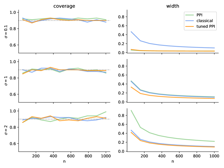
Figure 1: Mean estimation simulation study. The left column shows coverage, the right column shows confidence interval width. The top, middle, and bottom rows correspond to noise levels $\sigma=0.1$, $\sigma=1$, and $\sigma=2$, respectively.

Linear regression.

The goal is to estimate the coefficients of a linear regression model $Y=X^{\top}\theta+\epsilon$, where $X\sim\mathsf{N}(0,I_{d})$, $\theta\in\mathbb{R}^{d}$, and $\epsilon\sim\mathsf{N}(0,1)$, in dimension $d=2$. We use predictions $f(X_{i})=X_{i}^{\top}\theta+\epsilon_{i}$, where $\epsilon_{i}\sim\mathsf{N}(-2,\sigma^{2})$. We vary the noise level $\sigma\in\{0.1,0.5,1\}$, plotting results in Figure 2. The results are qualitatively similar to those in Figure 1: PPI++ adaptively interpolates between classical inference and standard PPI as the noise level changes, outperforming both.

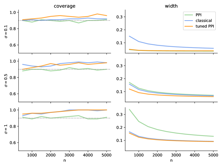
Figure 2: Linear regression simulation study. The left column shows coverage, the right column shows confidence interval width. The top, middle, and bottom rows correspond to noise levels $\sigma=0.1$, $\sigma=0.5$, and $\sigma=1$, respectively.

Logistic regression.

The goal is to estimate the coefficients of a logistic regression model, $\mathbb{P}(Y=1)=\mu_{\theta}(X)$, where $\mu_{\theta}(x)=\frac{e^{\theta^{\top}x}}{1+e^{\theta^{\top}x}}$ for $\theta\in\mathbb{R}^{d}$ with dimension $d=2$. We draw $X\sim\mathsf{N}(0,I_{d})$ and to simulate a binary classifier $f$ with error $\sigma$, we set the predictions $f(X_{i})$ to be $Y_{i}$ but randomly flipped with probability $\sigma$. We vary the flipping probability $\sigma\in\{0.01,0.1,0.2\}$, presenting results in Figure 3. As before, PPI++ successfully adapts to the varying noise in the predictions.

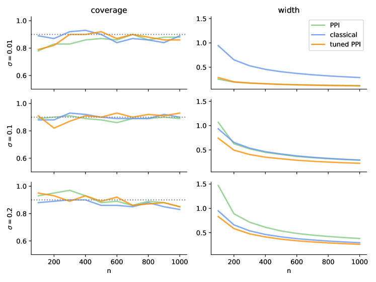
Figure 3: Logistic regression simulation study. The left column shows coverage, the right column shows confidence interval width. The top, middle, and bottom rows correspond to noise levels $\sigma=0.01$, $\sigma=0.1$, and $\sigma=0.2$, respectively.

7.1.2 Real data experiments

We now revisit five experiments on real data that Angelopoulos et al. perform [2], where we replicate their experimental settings, comparing to classical inferential approaches (that do not use the unlabeled data) as well.

Mean estimation on deforestation data.

The goal is to estimate the mean deforestation rate in the Amazon based on satellite imagery data [2]. The dataset includes $1596$ total pairs of observations and predictions, where the observations indicate whether deforestation occurred in a given randomly sampled region and the predictions are probits corresponding to these indicators. We take these predictions from the same gradient-boosted classifier as in [2], which is fit on a publicly available machine learning system that released tree canopy forest cover predictions at 30m resolution in the years 2000 and 2015. Generally, when the amount of forest cover in 2015 is substantially lower than in 2000, the model predicts that deforestation occurred.

Of the $1596$ total data points, we vary $n$, and then randomly take a labeled subset of size $n$ and use $N=1596-n$ as unlabeled. Figure 4 shows the results of the procedures over $100$ random splits into labeled and unlabeled data. For small $n$, PPI++ behaves similarly to standard PPI. When $n$ is large, meaning the unlabeled dataset size $N$ is small, classical inference outperforms standard PPI; PPI++ outperforms both.

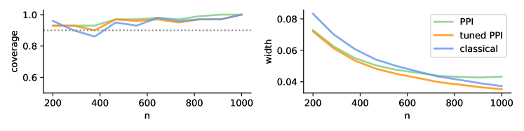
Figure 4: Mean estimation on deforestation data. The left panel shows coverage and the right shows width.

Mean estimation on galaxy data.

The goal is to estimate the fraction of spiral galaxies in the local universe based on images from the Sloan Digital Sky Survey (SDSS) and a pre-trained ResNet classifier, as in [2]. The scale of the universe makes human labeling of galaxies impossible, so scientists wish to use a computer-vision-based classifier to study the development of the universe. The classifier ingests images of galaxies and outputs an estimated probability that the galaxy is spiral. The dataset includes 1,364,122 total observations, of which we randomly take $n$ to serve as the labeled data and $N=1,\!364,\!122-n$ as the unlabeled data, for varying $n$. We show the results in Figure 5 over $100$ random splits into labeled and unlabeled data. As the predictions are very accurate in this problem, PPI++ and standard PPI are basically indistinguishable, and both are significantly more powerful than classical inference.

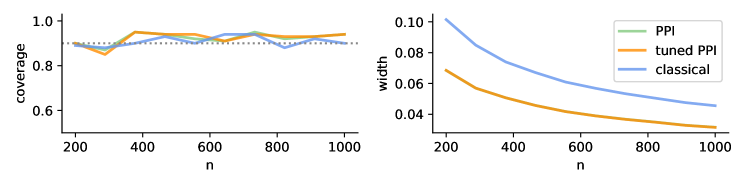
Figure 5: Mean estimation on galaxy data. The left panel shows coverage and the right shows width.

Linear regression on census data.

In this experiment, the goal is to estimate the coefficients of a linear regression model relating age (1-99) and sex (M/F) to income based on census data from California, as in [2]. We download the data through the Folktables [8] interface and use an XGBoost model [6] taking as input the ten covariates available in Folktables (including age, sex, the binary indicator of private health insurance) to produce predictions. We train the model on the entire census dataset in the year 2018 and use it to predict income for the year 2019. The 2019 data includes $377,\!575$ observations, of which we randomly take $n$ as labeled and $N=377,\!575-n$ as unlabeled, for varying $n$. We show the results in Figure 6 over $100$ random splits into labeled and unlabeled data. PPI++ is visually indistinguishable from standard PPI with $\lambda=1$.

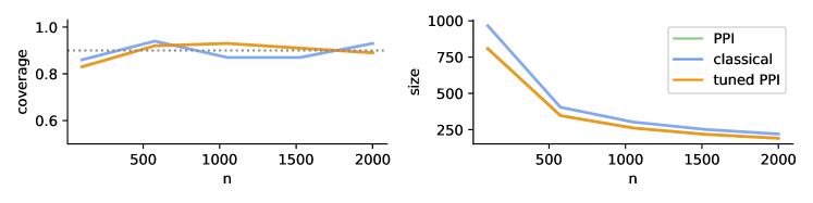
Figure 6: Linear regression on census data. The left panel shows coverage and the right shows width.

Logistic regression on census data.

The goal is to estimate the coefficients of a logistic regression model relating income ($) to the binary indicator of private health insurance based on census data. The setup otherwise resembles the previous experiment: we train an XGBoost model to predict income from ten other covariates, we have $377,\!575$ total observations, and so on. Figure 7 shows the results over $100$ random splits into labeled and unlabeled data. Tuned PPI behaves similarly to PPI, and both are more powerful than classical inference for all values of $n$.

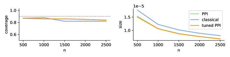
Figure 7: Logistic regression on census data. The left panel shows coverage and the right shows width.

7.2 Comparison to confidence sets from testing

The final comparison is to the naive implementation of prediction-powered inference [2, Algorithm 3]. We do not apply power tuning in this comparison as the goal is to understand the independent effect of the gridding procedure, which tests for “each” $\theta$ whether $\nabla L^{\mathrm{PP}}(\theta)=0$ is plausible, versus the technique proposed herein. The gridding means the original PPI method has much larger computational cost than the proposed method, while it is also less accurate (leading to larger sets, as in Figure 8). This follows because, to remain valid, the gridding method necessarily includes an extra grid point along each dimension. Furthermore, the method often outputs infinite sets because, in an effort to avoid an infinite runtime, the algorithm simply terminates grid refinement after a certain number of iterations. See Figure 8 for the median interval width for varying dimension $d$ and limit on the number of grid points before the algorithm returns an infinite set.

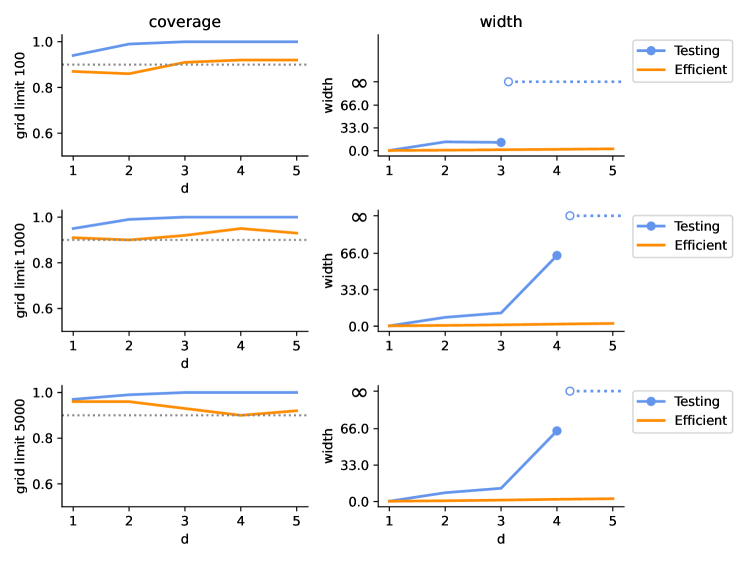
Figure 8: Comparison of PPI++ logistic regression, as in Algorithm 1, and standard PPI logistic regression [2, Algorithm 3]. The left panel shows coverage and the right shows width.

Appendix A Proofs

A.1 Proof of Theorem 1

We formally state the smoothness condition needed for Theorem 1.

Definition A.1 (Smooth enough losses).

The loss $\ell_{\theta}$ is smooth enough if

1. the losses $\ell_{\theta}(x,y)$ and $\ell_{\theta}(x,f(x))$ are differentiable at $\theta^{\star}$ for $\mathbb{P}$-almost every $(x,y)$,

2. the losses $\ell_{\theta}$ are locally Lipschitz around $\theta^{\star}$: there is a neighborhood of $\theta^{\star}$ such that $\ell_{\theta}(x,y)$ is $M(x,y)$-Lipschitz and $\ell_{\theta}(x,f(x))$ is $M(x)$-Lipschitz in $\theta$, where $\mathbb{E}[M(X,Y)^{2}+M(X)^{2}]<\infty$,

3. the population losses $L(\theta)=\mathbb{E}[\ell_{\theta}(X,Y)]$ and $L^{f}(\theta)=\mathbb{E}[\ell_{\theta}(X,f(X))]$ have Hessians $H_{\theta^{\star}}=\nabla^{2}L(\theta^{\star})\succ 0$ and $H_{\theta^{\star}}^{f}=\nabla^{2}L^{f}(\theta^{\star})$.

The proof follows that of van der Vaart [19, Theorem 5.23], with the modifications necessary to address the different observation model and empirical objective. Throughout the proof, we recall the labeling conventions that a tilde $\widetilde{\cdot}$ indicates the unlabeled sample $\{\widetilde{X}_{i}\}_{i=1}^{N}$ and a superscripted $f$ (i.e. $\cdot^{f}$) indicates using the machine-learning predictions $f$.

With this notational setting, given a function $g$, we use the shorthand notation

$$\mathbb{E}_{n}g :=\frac{1}{n}\sum_{i=1}^{n}g(X_{i},Y_{i}),\quad\mathbb{G}_{n}g=\sqrt{n}\left(\mathbb{E}_{n}g-\mathbb{E}[g(X,Y)]\right);$$ (9)

$$\widetilde{\mathbb{E}}_{N}^{f}g :=\frac{1}{N}\sum_{i=1}^{N}g(\widetilde{X}_{i},f_{i}(\widetilde{X}_{i})),\quad\widetilde{\mathbb{G}}_{N}^{f}g:=\sqrt{N}(\widetilde{\mathbb{E}}_{N}^{f}g-\mathbb{E}[g(X,f(X))]);$$ (10)

$$\mathbb{E}_{n}^{f}g :=\frac{1}{n}\sum_{i=1}^{n}g(X_{i},f(X_{i})),\quad\mathbb{G}_{n}^{f}g:=\sqrt{n}(\mathbb{E}_{n}^{f}g-\mathbb{E}[g(X,f(X))]).$$ (11)

The differentiability of $\ell_{\theta}(x,y)$ and $\ell_{\theta}(x,f(x))$ at $\theta^{\star}$ (Definition A.1(i)) and the local Lipschitzness of the losses (Definition A.1(ii)) imply that for every (possibly random) sequence $h_{n}=O_{P}(1)$, we have

$$\mathbb{G}\left[\sqrt{n}\left(\ell_{\theta^{\star}+\frac{h_{n}}{\sqrt{n}}}-\ell_{\theta^{\star}}\right)-h_{n}^{\top}\nabla\ell_{\theta^{\star}}\right]\stackrel{{\scriptstyle p}}{{\rightarrow}}0$$

for any of the empirical processes $\mathbb{G}\in\{\mathbb{G}_{n},\widetilde{\mathbb{G}}_{N}^{f},\mathbb{G}_{n}^{f}\}$ (see [19, Lemma 19.31]). By applying a second-order Taylor expansion, this implies

$$n\mathbb{E}_{n}\left(\ell_{\theta^{\star}+\frac{h_{n}}{\sqrt{n}}}-\ell_{\theta^{\star}}\right) =n\left(L\Big{(}\theta^{\star}+\frac{h_{n}}{\sqrt{n}}\Big{)}-L(\theta^{\star})\right)+h_{n}^{\top}\mathbb{G}_{n}\nabla\ell_{\theta^{\star}}+o_{P}(1)$$

$$=\frac{1}{2}h_{n}^{\top}H_{\theta^{\star}}h_{n}+h_{n}^{\top}\mathbb{G}_{n}\nabla\ell_{\theta^{\star}}+o_{P}(1).$$

Similarly, we have the two equalities

$$\hat{\lambda}n\widetilde{\mathbb{E}}_{N}^{f}\left(\ell_{\theta^{\star}+\frac{h_{n}}{\sqrt{n}}}-\ell_{\theta^{\star}}\right) =(\lambda+o_{P}(1))\left(\frac{1}{2}h_{n}^{\top}H_{\theta^{\star}}^{f}h_{n}+\sqrt{\frac{n}{N}}h_{n}^{\top}\widetilde{\mathbb{G}}_{N}^{f}\nabla\ell_{\theta^{\star}}+o_{P}(1)\right)$$

$$=\lambda\left(\frac{1}{2}h_{n}^{\top}H_{\theta^{\star}}^{f}h_{n}+\sqrt{\frac{n}{N}}h_{n}^{\top}\widetilde{\mathbb{G}}_{N}^{f}\nabla\ell_{\theta^{\star}}\right)+o_{P}(1),~{}~{}\mbox{and}$$

$$-\hat{\lambda}n\mathbb{E}_{n}^{f}\left(\ell_{\theta^{\star}+\frac{h_{n}}{\sqrt{n}}}-\ell_{\theta^{\star}}\right) =(\lambda+o_{P}(1))\left(-\frac{1}{2}h_{n}^{\top}H_{\theta^{\star}}^{f}h_{n}-h_{n}^{\top}\mathbb{G}_{n}^{f}\nabla\ell_{\theta^{\star}}+o_{P}(1)\right)$$

$$=\lambda\left(-\frac{1}{2}h_{n}^{\top}H_{\theta^{\star}}^{f}h_{n}-h_{n}^{\top}\mathbb{G}_{n}^{f}\nabla\ell_{\theta^{\star}}\right)+o_{P}(1).$$

Adding the preceding three equations and recalling the definition that

$$L^{\mathrm{PP}}_{\lambda}(\theta)=\mathbb{E}_{n}\ell_{\theta}+\lambda(\widetilde{\mathbb{E}}_{N}^{f}\ell_{\theta}-\mathbb{E}_{n}^{f}\ell_{\theta}),$$

we have

$$n\left(L^{\mathrm{PP}}_{\hat{\lambda}}\left(\theta^{\star}+\frac{h_{n}}{\sqrt{n}}\right)-L^{\mathrm{PP}}_{\hat{\lambda}}(\theta^{\star})\right)=\frac{1}{2}h_{n}^{\top}H_{\theta^{\star}}h_{n}+h_{n}^{\top}\left(\mathbb{G}_{n}\nabla\ell_{\theta^{\star}}+\lambda\sqrt{\frac{n}{N}}\widetilde{\mathbb{G}}_{N}^{f}\nabla\ell_{\theta^{\star}}-\lambda\mathbb{G}_{n}^{f}\nabla\ell_{\theta^{\star}}\right)+o_{P}(1).$$

We now evaluate this expression for two particular choices of the sequence $h_{n}$. First, consider $h_{n}^{\star}=\sqrt{n}(\hat{\theta}^{\mathrm{PP}}_{\hat{\lambda}}-\theta^{\star})$. Because the losses are smooth enough (Definition A.1), $\theta\mapsto\lambda\ell_{\theta}$ is locally Lipschitz uniformly for $\lambda$ in (any) compact set, and so the consistency $\hat{\theta}^{\mathrm{PP}}_{\hat{\lambda}}\to\theta^{\star}$ implies that $h_{n}^{\star}=O_{P}(1)$ (van der Vaart [19, Corollary 5.53]). This yields

$$n\left(L^{\mathrm{PP}}_{\hat{\lambda}}(\hat{\theta}^{\mathrm{PP}}_{\hat{\lambda}})-L^{\mathrm{PP}}_{\hat{\lambda}}(\theta^{\star})\right)=\frac{1}{2}{h_{n}^{\star}}^{\top}H_{\theta^{\star}}h_{n}^{\star}+{h_{n}^{\star}}^{\top}\left(\mathbb{G}_{n}\nabla\ell_{\theta^{\star}}+\lambda\sqrt{\frac{n}{N}}\widetilde{\mathbb{G}}_{N}^{f}\nabla\ell_{\theta^{\star}}-\lambda\mathbb{G}_{n}^{f}\nabla\ell_{\theta^{\star}}\right)+o_{P}(1).$$

We can perform a similar expansion with $h_{n}=-H_{\theta^{\star}}^{-1}(\mathbb{G}_{n}\nabla\ell_{\theta^{\star}}+\lambda\sqrt{\frac{n}{N}}\widetilde{\mathbb{G}}_{N}^{f}\nabla\ell_{\theta^{\star}}-\lambda\mathbb{G}_{n}^{f}\nabla\ell_{\theta^{\star}})$, which is certainly $O_{P}(1)$, yielding

$$n\left(L^{\mathrm{PP}}_{\hat{\lambda}}(\theta^{\star}-h_{n}/\sqrt{n})-L^{\mathrm{PP}}_{\hat{\lambda}}(\theta^{\star})\right)=-\frac{1}{2}h_{n}^{\top}H_{\theta^{\star}}h_{n}+o_{P}(1).$$

By the definition of $\hat{\theta}^{\mathrm{PP}}_{\hat{\lambda}}$, the left-hand side of the first equation is smaller than the left-hand side of the second equation, and so

$$\frac{1}{2}{h_{n}^{\star}}^{\top}H_{\theta^{\star}}h_{n}^{\star}-{h_{n}^{\star}}^{\top}H_{\theta^{\star}}h_{n}\leq-\frac{1}{2}h_{n}^{\top}H_{\theta^{\star}}h_{n}+o_{P}(1),$$

or, rearranging,

$$\frac{1}{2}(h_{n}^{\star}-h_{n})^{\top}H_{\theta^{\star}}(h_{n}^{\star}-h_{n})=o_{P}(1).$$

As $H_{\theta^{\star}}$ is positive definite, we thus must have $h_{n}^{\star}=h_{n}+o_{P}(1)$, that is,

$$\sqrt{n}\left(\hat{\theta}^{\mathrm{PP}}_{\hat{\lambda}}-\theta^{\star}\right)=-H_{\theta^{\star}}^{-1}\left(\mathbb{G}_{n}\nabla\ell_{\theta^{\star}}+\lambda\sqrt{\frac{n}{N}}\widetilde{\mathbb{G}}_{N}^{f}\nabla\ell_{\theta^{\star}}-\lambda\mathbb{G}_{n}^{f}\nabla\ell_{\theta^{\star}}\right)+o_{P}(1).$$

It remains to demonstrate the asymptotic normality of the empirical processes on the right-hand side. This follows by the central limit theorem:

$$\mathbb{G}_{n}\nabla\ell_{\theta^{\star}}+\lambda\sqrt{\frac{n}{N}}\widetilde{\mathbb{G}}_{N}^{f}\nabla\ell_{\theta^{\star}}-\lambda\mathbb{G}_{n}^{f}\nabla\ell_{\theta^{\star}}$$

$$\quad=\lambda\sqrt{\frac{n}{N}}\cdot\frac{1}{\sqrt{N}}\sum_{i=1}^{N}(\nabla\tilde{\ell}_{\theta^{\star},i}^{f}-\mathbb{E}[\nabla\ell_{\theta^{\star}}^{f}])+\frac{1}{\sqrt{n}}\sum_{i=1}^{n}\left(\nabla\ell_{\theta^{\star},i}-\lambda\nabla\ell_{\theta^{\star},i}^{f}-\mathbb{E}[\nabla\ell_{\theta^{\star}}-\lambda\nabla\ell_{\theta^{\star}}^{f}]\right)$$

$$\quad\mathop{\stackrel{{\scriptstyle d}}{{\rightarrow}}}\mathsf{N}\left(0,\lambda^{2}r\cdot\mathrm{Var}(\nabla\ell_{\theta^{\star}}^{f})+\mathrm{Var}(\nabla\ell_{\theta^{\star}}-\lambda\nabla\ell_{\theta^{\star}}^{f})\right).$$

Thus $H_{\theta^{\star}}^{-1}\left(\mathbb{G}_{n}\nabla\ell_{\theta^{\star}}+\lambda\sqrt{\frac{n}{N}}\widetilde{\mathbb{G}}_{N}^{f}\nabla\ell_{\theta^{\star}}-\lambda\mathbb{G}_{n}^{f}\nabla\ell_{\theta^{\star}}\right)\mathop{\stackrel{{\scriptstyle d}}{{\rightarrow}}}\mathsf{N}(0,\Sigma^{\lambda})$, completing the proof.

A.2 Proof of Proposition 1

We begin by stating an auxiliary lemma.

Lemma A.1.

Let $g:\mathbb{R}^{d}\to\mathbb{R}$ be a convex function. Fix $\theta_{0},\theta_{1}\in\mathbb{R}^{d}$ and $t\geq 1$, and define $\theta_{t}=\theta_{0}+t(\theta_{1}-\theta_{0})$. Then $g(\theta_{t})\geq g(\theta_{0})+t(g(\theta_{1})-g(\theta_{0}))$.

Proof.

Rearranging terms, we have $\theta_{1}=\frac{1}{t}\theta_{t}+(1-\frac{1}{t})\theta_{0}$ . Applying the definition of convexity at $\theta_{1}$ gives

$$g(\theta_{1})\leq\frac{1}{t}g(\theta_{t})+\left(1-\frac{1}{t}\right)g(\theta_{0}),$$

which is equivalent to $g(\theta_{t})\geq g(\theta_{0})+t(g(\theta_{1})-g(\theta_{0}))$. ∎

Returning to Proposition 1, the local Lipschitzness condition implies there is an $\epsilon>0$ such that

$$\sup_{\theta:\|\theta-\theta^{\star}\|\leq\epsilon}|L^{\mathrm{PP}}_{\lambda}(\theta)-L(\theta)|\stackrel{{\scriptstyle p}}{{\rightarrow}}0$$ (12)

by a standard covering argument. By the uniqueness of $\theta^{\star}$, for all $\epsilon>0$ we know there exists a $\delta>0$ such that $L(\theta)-L(\theta^{\star})\geq\delta$ for all $\theta$ on the $\epsilon$-shell $\{\theta\mid\left\|{\theta-\theta^{\star}}\right\|=\epsilon\}$ around $\theta^{\star}$. With this we can write

$$\inf_{\left\|{\theta-\theta^{\star}}\right\|=\epsilon}L^{\mathrm{PP}}_{\lambda}(\theta)-L^{\mathrm{PP}}_{\lambda}(\theta^{\star}) =\inf_{\left\|{\theta-\theta^{\star}}\right\|=\epsilon}\left((L^{\mathrm{PP}}_{\lambda}(\theta)-L(\theta)+(L(\theta)-L(\theta^{\star}))+(L(\theta^{\star})-L^{\mathrm{PP}}_{\lambda}(\theta^{\star}))\right)$$

$$\geq\delta-o_{P}(1),$$

where the convergence (12) guarantees that the first and third terms above vanish.

Now fix any $\theta$ such that $\left\|{\theta-\theta^{\star}}\right\|\geq\epsilon$. We apply Lemma A.1 with $\theta_{0}=\theta^{\star}$ and $\theta_{1}=\frac{\theta-\theta^{\star}}{\|\theta-\theta^{\star}\|}\epsilon$. Combining the preceding display with Lemma A.1 gives

$$L^{\mathrm{PP}}_{\lambda}(\theta)-L^{\mathrm{PP}}_{\lambda}(\theta^{\star})\geq\frac{\|\theta-\theta^{\star}\|}{\epsilon}(\delta-o_{P}(1))\geq\delta-o_{P}(1).$$

Therefore, no $\theta$ with $\|\theta-\theta^{\star}\|\geq\epsilon$ can minimize $L^{\mathrm{PP}}_{\lambda}$, and so by contradiction we have shown $\mathbb{P}(\|{\hat{\theta}^{\mathrm{PP}}_{\lambda}-\theta^{\star}}\|<\epsilon)\to 1$, as desired.

We turn to the final claim of the proposition, which allows random $\hat{\lambda}$. The convergence (12) holds uniformly for $\lambda^{\prime}$ in a small neighborhood of $\lambda$ as well because of an identical covering argument; as $\hat{\lambda}=\lambda+o_{P}(1)$, with probability tending to 1 we have that $\hat{\lambda}$ belongs to the neighborhood of $\lambda$. The rest of the proof is identical.

A.3 Proof of Theorem 2

We will require that the loss function is stochastically smooth in the following sense.

Assumption A1 (Stochastic smoothness).

There exists a compact neighborhood $B$ of $\theta^{\star}$ such that the classes

$$\mathcal{L}:=\{(x,y)\mapsto\nabla\ell_{\theta}(x,y):\theta\in B\}~{}~{}~{}\mbox{and}~{}~{}~{}\mathcal{L}^{f}:=\{x\mapsto\nabla\ell_{\theta}(x,f(x)):\theta\in B\}$$

are both $\mathbb{P}$-Donsker.

Let $Z\sim\mathsf{N}(0,I)$. We will show that, for any $c<\infty$,

$$\limsup_{n}\sup_{\left\|{h}\right\|\leq c}\left|\mathbb{P}(\theta^{\star}+h/\sqrt{n}\in\mathcal{C}^{\mathrm{PP}}_{\alpha})-\mathbb{P}\big{(}\big{\|}{-\Sigma^{-1/2}h+Z}\big{\|}_{2}^{2}\leq\chi^{2}_{d,1-\alpha}\big{)}\right|=0,$$ (13)

for $\mathcal{C}^{\mathrm{PP}}_{\alpha}\in\{\mathcal{C}_{\alpha}^{\mathrm{PP},T},\mathcal{C}_{\alpha}^{\mathrm{PP},U}\}$, where $\Sigma$ is the asymptotic covariance from Theorem 1 for $\lambda=1$, i.e. $\Sigma\equiv\Sigma^{1}=H_{\theta^{\star}}^{-1}(rV^{1}_{f,\theta^{\star}}+V^{1}_{\Delta,\theta^{\star}})H_{\theta^{\star}}^{-1}$.

The result (13) directly implies the main result of the theorem.

Let $h_{n}$ be any sequence such that $\sqrt{n}h_{n}\to h$ for some fixed $h\in\mathbb{R}^{d}$. We give alternative representations of the statistics $T_{n}$ and $U_{n}$ under the local alternative parameters $\theta^{\star}+h_{n}$. We leverage the following two technical lemmas:

Lemma A.2.

Under the conditions of Theorem 2,

$$\widehat{V}_{\Delta}(\theta^{\star}+h_{n})\stackrel{{\scriptstyle p}}{{\rightarrow}}{\rm Var}(\nabla\ell_{\theta^{\star}}-\nabla\ell_{\theta^{\star}}^{f})~{}~{}\mbox{and}~{}~{}\widehat{V}_{f}(\theta^{\star}+h_{n})\stackrel{{\scriptstyle p}}{{\rightarrow}}{\rm Var}(\nabla\ell_{\theta^{\star}}^{f}).$$

Lemma A.3.

Define the (sub)gradient process

$$\widehat{G}(\theta):=\mathbb{E}_{n}[\nabla\ell_{\theta}-\nabla\ell_{\theta}^{f}]-\mathbb{E}[\nabla\ell_{\theta}-\nabla\ell_{\theta}^{f}]+\widetilde{\mathbb{E}}_{N}[\nabla\ell_{\theta}^{f}]-\mathbb{E}[\nabla\ell_{\theta}^{f}].$$ (14)

Then, under the conditions of Theorem 2, $\widehat{G}(\theta^{\star}+h_{n})=\widehat{G}(\theta^{\star})+o_{P}(1/\sqrt{n}).$

Lemma A.2 follows by the classical result [20, Lemma 2.10.14] that if $\mathcal{F}$ is a Donsker class, then $\mathcal{F}^{2}=\{f^{2}:f\in\mathcal{F}\}$ is Glivenko-Cantelli.

Lemma A.3 follows by the fact that the process is asymptotically stochastically equicontinuous, which follows by Assumption A1; see below for the proof.

Proof of Lemma A.3.

We adopt the definitions of $\mathbb{G}_{n}g$, $\mathbb{G}_{N}^{f}g$, and $\mathbb{G}_{n}^{f}g$ from Equations (9), (10), and (11), respectively. Because the process $[\mathbb{G}_{n}\nabla\ell_{\theta}]_{\theta\in B}$ converges to a (tight) Gaussian process in $\theta$ by Assumption A1, as $h_{n}=O_{P}(1/\sqrt{n})$ we necessarily have

$$\mathbb{G}_{n}\nabla\ell_{\theta^{\star}+h_{n}}-\mathbb{G}_{n}\nabla\ell_{\theta^{\star}}\stackrel{{\scriptstyle p}}{{\rightarrow}}0$$

(as the process is asymptotically stochastically equicontinuous by Assumption A1). Similarly, Assumption A1 implies $\mathbb{G}_{N}^{f}\nabla\ell_{\theta^{\star}+h_{n}}-\mathbb{G}_{N}^{f}\nabla\ell_{\theta^{\star}}\stackrel{{\scriptstyle p}}{{\rightarrow}}0$ and $\mathbb{G}_{n}^{f}\nabla\ell_{\theta^{\star}+h_{n}}-\mathbb{G}_{n}^{f}\nabla\ell_{\theta^{\star}}\stackrel{{\scriptstyle p}}{{\rightarrow}}0$. Adding and subtracting the preceding quantities and rescaling by $\sqrt{n}$, we obtain the lemma. ∎

Now we give asymptotically equivalent formulations of $T_{n}$ and $U_{n}$ evaluated at the alternatives $\theta^{\star}+h_{n}$. We can write $T_{n}$ as

$$T_{n}(\theta^{\star}+h_{n})=\sqrt{n}\widehat{\Sigma}^{-1/2}(\hat{\theta}^{\mathrm{PP}}-\theta^{\star}-h_{n})=\sqrt{n}\widehat{\Sigma}^{-1/2}(\hat{\theta}^{\mathrm{PP}}-\theta^{\star})-\Sigma^{-1/2}h+o_{P}(1).$$

Turning to $U_{n}$, we let $V_{\Delta,\theta^{\star}}={\rm Var}(\nabla\ell_{\theta^{\star}}-\nabla\ell_{\theta^{\star}}^{f})$ and $V_{f,\theta^{\star}}={\rm Var}(\nabla\ell_{\theta^{\star}}^{f})$. Then Lemma A.2 and Lemma A.3 give

$$U_{n}(\theta^{\star}+h_{n})$$

$$\quad\stackrel{{\scriptstyle(i)}}{{=}}\sqrt{n}(V_{\Delta,\theta^{\star}}+\ratio V_{f,\theta^{\star}}+o_{P}(1))^{-1/2}\widehat{G}(\theta^{\star}+h_{n})+\sqrt{n}(V_{\Delta,\theta^{\star}}+\ratio V_{f,\theta^{\star}}+o_{P}(1))^{-1/2}\nabla L(\theta^{\star}+h_{n})$$

$$\quad\stackrel{{\scriptstyle(ii)}}{{=}}\sqrt{n}(V_{\Delta,\theta^{\star}}+\ratio V_{f,\theta^{\star}})^{-1/2}\widehat{G}(\theta^{\star})+(V_{\Delta,\theta^{\star}}+\ratio V_{f,\theta^{\star}})^{-1/2}H_{\theta^{\star}}h+o_{P}(1),$$

where step $(i)$ follows from Lemma A.2 and $(ii)$ from Lemma A.3 coupled with Slutsky’s lemmas and that $\nabla L(\theta^{\star}+h_{n})=\nabla L(\theta^{\star}+h_{n})-\nabla L(\theta^{\star})=\nabla^{2}L(\theta^{\star})h_{n}+o(\left\|{h_{n}}\right\|)=H_{\theta^{\star}}h_{n}+o(1/\sqrt{n})$.

Rewriting the preceding two displays and applying Theorem 1 to the first, we have

$$T_{n}(\theta^{\star}+h_{n})\mathop{\stackrel{{\scriptstyle d}}{{\rightarrow}}}\mathsf{N}(-\Sigma^{-1/2}h,I)~{}~{}\mbox{and}~{}~{}U_{n}(\theta^{\star}+h_{n})\mathop{\stackrel{{\scriptstyle d}}{{\rightarrow}}}\mathsf{N}((V_{\Delta,\theta^{\star}}+\ratio V_{f,\theta^{\star}})^{-1/2}H_{\theta^{\star}}h,I).$$

The squared norm of the latter mean satisfies

$$\left\|{(V_{\Delta,\theta^{\star}}+\ratio V_{f,\theta^{\star}})^{-1/2}H_{\theta^{\star}}h}\right\|_{2}^{2}=h^{T}H_{\theta^{\star}}(V_{\Delta,\theta^{\star}}+\ratio V_{f,\theta^{\star}})^{-1}H_{\theta^{\star}}h=h^{T}\Sigma^{-1}h$$

by the definition of $\Sigma$. Therefore, the rotational invariance of the Gaussian yields

$$\begin{split}\mathbb{P}(\theta^{\star}+h_{n}\in\mathcal{C}_{\alpha}^{\mathrm{PP},T})&=\mathbb{P}(\left\|{T_{n}(\theta^{\star}+h_{n})}\right\|_{2}^{2}\leq\chi^{2}_{d,1-\alpha})=\mathbb{P}\left(\left\|{-\Sigma^{-1/2}h+Z}\right\|_{2}^{2}\leq\chi^{2}_{d,1-\alpha}\right)+o(1)\\ \mathbb{P}(\theta^{\star}+h_{n}\in\mathcal{C}_{\alpha}^{\mathrm{PP},U})&=\mathbb{P}(\left\|{U_{n}(\theta^{\star}+h_{n})}\right\|_{2}^{2}\leq\chi^{2}_{d,1-\alpha})=\mathbb{P}\left(\left\|{-\Sigma^{-1/2}h+Z}\right\|_{2}^{2}\leq\chi^{2}_{d,1-\alpha}\right)+o(1),\end{split}$$ (15)

where $Z\sim\mathsf{N}(0,I)$.

Finally, we employ a standard compactification argument. Assume for the sake of contradiction that

$$\limsup_{n}\sup_{\left\|{h}\right\|\leq c}\left|\mathbb{P}(\theta^{\star}+h/\sqrt{n}\in\mathcal{C}^{\mathrm{PP}}_{\alpha})-\mathbb{P}\left(\left\|{-\Sigma^{-1/2}h+Z}\right\|_{2}^{2}\leq\chi^{2}_{d,1-\alpha}\right)\right|>0,$$

for one of $\mathcal{C}^{\mathrm{PP}}_{\alpha}\in\{\mathcal{C}_{\alpha}^{\mathrm{PP},T},\mathcal{C}_{\alpha}^{\mathrm{PP},U}\}$. If this is the case, then there must be a bounded subsequence of $h_{n}$ with

$$\left|\mathbb{P}(\theta^{\star}+h_{n}/\sqrt{n}\in\mathcal{C}^{\mathrm{PP}}_{\alpha})-\mathbb{P}\left(\left\|{-\Sigma^{-1/2}h_{n}+Z}\right\|_{2}^{2}\leq\chi^{2}_{d,1-\alpha}\right)\right|\to a>0.$$

Take a convergent subsequence from this set, so that $\sqrt{n}(h_{n}/\sqrt{n})=h_{n}\to h$. The existence of this subsequence contradicts the limits (15). This proves the first claim of the theorem.

For the second claim, take any $t_{n}=\omega(1/\sqrt{n})$ and $\delta\in(0,1)$. Then

$$\mathbb{P}\left(\theta^{\star}+ht_{n}\in\mathcal{C}_{\alpha}^{\mathrm{PP},T}\right) \leq\mathbb{P}\left(\|\sqrt{n}\widehat{\Sigma}^{-1/2}ht_{n}\|\leq\chi_{d,1-\alpha}+\|\sqrt{n}\widehat{\Sigma}^{-1/2}(\hat{\theta}^{\mathrm{PP}}-\theta^{\star})\|\right)$$

$$\leq\mathbb{P}\left(\|\sqrt{n}\widehat{\Sigma}^{-1/2}ht_{n}\|\leq\chi_{d,1-\alpha}+\chi_{d,1-\delta}\right)+\mathbb{P}\left(\|\sqrt{n}\widehat{\Sigma}^{-1/2}(\hat{\theta}^{\mathrm{PP}}-\theta^{\star})\|>\chi_{d,1-\delta}\right).$$

Taking the limit, we get

$$\limsup_{n}\sup_{\|h\|\geq c}\mathbb{P}\left(\theta^{\star}+ht_{n}\in\mathcal{C}_{\alpha}^{\mathrm{PP},T}\right)\leq\delta.$$

As $\delta$ was arbitrary, we conclude that $\limsup_{n}\sup_{\|h\|\geq c}\mathbb{P}(\theta^{\star}+ht_{n}\in\mathcal{C}_{\alpha}^{\mathrm{PP},T})=0$.

A.4 Proof of Proposition 2

By definition

$$\lambda^{\star}=\operatorname*{arg\,min}_{\lambda}\mathrm{Tr}\left(\Sigma^{\lambda}\right)=\operatorname*{arg\,min}_{\lambda}\mathrm{Tr}\left(H_{\theta^{\star}}^{-1}\left(r\cdot\lambda^{2}\mathrm{Var}(\nabla\ell_{\theta^{\star}}^{f})+\mathrm{Var}(\nabla\ell_{\theta^{\star}}-\lambda\nabla\ell_{\theta^{\star}}^{f})\right)H_{\theta^{\star}}^{-1}\right).$$

Writing $\textup{Cov}(\nabla\ell_{\theta^{\star}}-\lambda\nabla\ell_{\theta^{\star}}^{f})=\textup{Cov}(\nabla\ell_{\theta^{\star}})+\lambda^{2}\textup{Cov}(\nabla\ell_{\theta^{\star}}^{f})-\lambda(\mathrm{Cov}(\nabla\ell_{\theta^{\star}},\nabla\ell_{\theta^{\star}}^{f})+\mathrm{Cov}(\nabla\ell_{\theta^{\star}}^{f},\nabla\ell_{\theta^{\star}}))$ and applying the linearity of the trace, $\lambda^{\star}$ evidently minimizes

$$\lambda^{2}(1+r)\mathrm{Tr}\left(H_{\theta^{\star}}^{-1}\mathrm{Var}(\nabla\ell_{\theta^{\star}}^{f})H_{\theta^{\star}}^{-1}\right)-\lambda\mathrm{Tr}\left(H_{\theta^{\star}}^{-1}\left(\mathrm{Cov}\left(\nabla\ell_{\theta^{\star}},\nabla\ell_{\theta^{\star}}^{f}\right)+\mathrm{Cov}\left(\nabla\ell_{\theta^{\star}}^{f},\nabla\ell_{\theta^{\star}}\right)\right)H_{\theta^{\star}}^{-1}\right).$$

Analytically optimizing this quadratic gives the optimal choice

$$\lambda^{\star}=\frac{\mathrm{Tr}\left(H_{\theta^{\star}}^{-1}\left(\mathrm{Cov}\left(\nabla\ell_{\theta^{\star}},\nabla\ell_{\theta^{\star}}^{f}\right)+\mathrm{Cov}\left(\nabla\ell_{\theta^{\star}}^{f},\nabla\ell_{\theta^{\star}}\right)\right)H_{\theta^{\star}}^{-1}\right)}{2(1+r)\mathrm{Tr}\left(H_{\theta^{\star}}^{-1}\mathrm{Var}(\nabla\ell_{\theta^{\star}}^{f})H_{\theta^{\star}}^{-1}\right)}.$$

Appendix B Experiments with one-step PPI

We repeat the synthetic experiments from the main text (Section 7.1.1), but only compare PPI (with $\lambda=1$), power-tuned PPI (PPI++) with clipping $\hat{\lambda}$ to $[0,1]$, and one-step PPI. The figures below show the results in sequence; one-step PPI and power-tuned PPI overlap almost completely in all plots but one: Figure 10. This figure shows results from a new experiment using anticorrelated predictions (the same setting as in Figure 1, except that we take $f(X_{i})=-Y_{i}+\epsilon$). In this setting, one-step PPI outperforms PPI and power-tuned PPI because it allows $\hat{\lambda}$ to be negative.

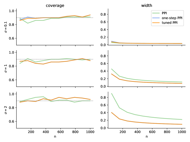
Figure 9: Mean estimation with one-step PPI. The left panel shows coverage and the right shows width. The setup is the same as in Figure 1.

Figure 10: Mean estimation with one-step PPI and anticorrelated predictions. The left panel shows coverage and the right shows width. The setup is the same as in Figure 1, only we multiply the true outcomes by $-1$ when generating the predictions, $f(X_{i})=-Y_{i}+\epsilon$.

Figure 11: Linear regression with one-step PPI. The left panel shows coverage and the right shows width. The setup is the same as in Figure 2.

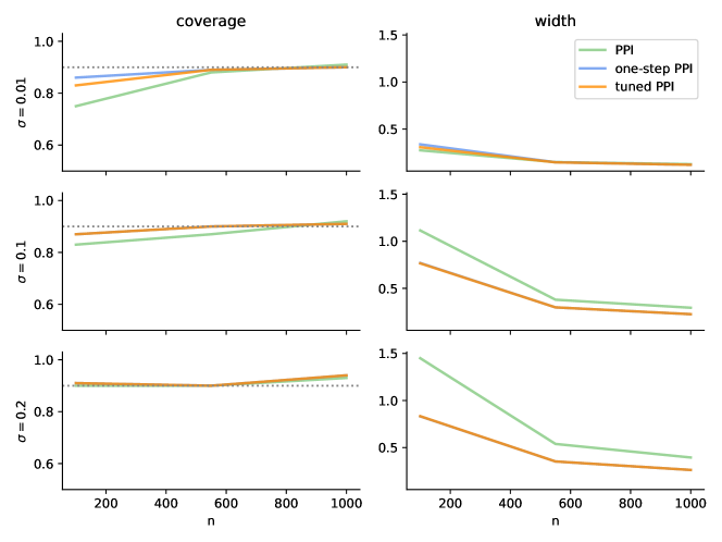
Figure 12: Logistic regression with one-step PPI. The left panel shows coverage and the right shows width. The setup is the same as in Figure 3.

References

- Angelopoulos et al. [2023a] A. Angelopoulos, J. C. Duchi, and T. Zrnic. A note on statistical efficiency in Prediction-Powered Inference. 2023a. URL https://web.stanford.edu/~jduchi/projects/AngelopoulosDuZr23w.pdf.
- Angelopoulos et al. [2023b] A. N. Angelopoulos, S. Bates, C. Fannjiang, M. I. Jordan, and T. Zrnic. Prediction-powered inference. arXiv:2301.09633, 2023b.
- Bickel et al. [1998] P. Bickel, C. A. J. Klaassen, Y. Ritov, and J. Wellner. Efficient and Adaptive Estimation for Semiparametric Models. Springer Verlag, 1998.
- Boyd and Vandenberghe [2004] S. Boyd and L. Vandenberghe. Convex Optimization. Cambridge University Press, 2004.
- Brown [1986] L. D. Brown. Fundamentals of Statistical Exponential Families. Institute of Mathematical Statistics, Hayward, California, 1986.
- Chen and Guestrin [2016] T. Chen and C. Guestrin. XGBoost: A scalable tree boosting system. In Proceedings of the 22nd ACM SIGKDD Conference on Knowledge Discovery and Data Mining (KDD), pages 785–794, 2016.
- Chernozhukov et al. [2018] V. Chernozhukov, D. Chetverikov, M. Demirer, E. Duflo, C. Hansen, W. Newey, and J. Robins. Double/debiased machine learning for treatment and structural parameters. The Econometrics Journal, 21(1):C1–C68, 2018.
- Ding et al. [2021] F. Ding, M. Hardt, J. Miller, and L. Schmidt. Retiring Adult: New datasets for fair machine learning. Advances in Neural Information Processing Systems 34, 2021.
- Efron [2022] B. Efron. Exponential Families in Theory and Practice. Cambridge University Press, 2022.
- Jumper et al. [2021] J. Jumper, R. Evans, A. Pritzel, T. Green, M. Figurnov, K. Tunyasuvunakool, O. Ronneberger, R. Bates, A. Zidek, A. Bridgland, C. Meyer, S. A. A. Kohl, A. Potapenko, A. J. Ballard, A. Cowie, B. Romera-Paredes, S. Nikolov, R. Jain, J. Adler, T. Back, S. Petersen, D. Reiman, M. Steinegger, M. Pacholska, D. Silver, O. Vinyals, A. W. Senior, K. Kavukcuoglu, P. Kohli, and D. Hassabis. Highly accurate protein structure prediction with AlphaFold. Nature, 596:583–589, 2021.
- LeCun et al. [2015] Y. LeCun, Y. Bengio, and G. Hinton. Deep learning. Nature, 521(7553):436–444, 2015.
- Radford et al. [2021] A. Radford, J. W. Kim, C. Hallacy, A. Ramesh, G. Goh, S. Agarwal, G. Sastry, A. Askell, P. Mishkin, J. Clark, G. Krueger, and I. Sutskever. Learning transferable visual models from natural language supervision. In Proceedings of the 38th International Conference on Machine Learning, 2021.
- Robins and Rotnitzky [1995] J. M. Robins and A. Rotnitzky. Semiparametric efficiency in multivariate regression models with missing data. Journal of the American Statistical Association, 90(429):122–129, 1995.
- Robins et al. [1994] J. M. Robins, A. Rotnitzky, and L. P. Zhao. Estimation of regression coefficients when some regressors are not always observed. Journal of the American Statistical Association, 89(427):846–866, 1994.
- Rubin [2018] D. B. Rubin. Multiple imputation. In Flexible Imputation of Missing Data, Second Edition, pages 29–62. Chapman and Hall/CRC, 2018.
- Särndal et al. [2003] C.-E. Särndal, B. Swensson, and J. Wretman. Model assisted survey sampling. Springer Science & Business Media, 2003.
- Song et al. [2023] S. Song, Y. Lin, and Y. Zhou. A general m-estimation theory in semi-supervised framework. Journal of the American Statistical Association, pages 1–11, 2023.
- Tsiatis [2006] A. Tsiatis. Semiparametric Theory and Missing Data. Springer, 2006.
- van der Vaart [1998] A. W. van der Vaart. Asymptotic Statistics. Cambridge Series in Statistical and Probabilistic Mathematics. Cambridge University Press, 1998.
- van der Vaart and Wellner [1996] A. W. van der Vaart and J. A. Wellner. Weak Convergence and Empirical Processes: With Applications to Statistics. Springer, New York, 1996.
- Zhang et al. [2019] A. Zhang, L. D. Brown, and T. T. Cai. Semi-supervised inference: General theory and estimation of means. The Annals of Statistics, 47:2538–2566, 2019.
- Zhang and Bradic [2022] Y. Zhang and J. Bradic. High-dimensional semi-supervised learning: in search of optimal inference of the mean. Biometrika, 109(2):387–403, 2022.