Tailoring Mixup to Data using Kernel Warping functions

Abstract

Data augmentation is an essential building block for learning efficient deep learning models. Among all augmentation techniques proposed so far, linear interpolation of training data points, also called mixup, has found to be effective for a large panel of applications. While the majority of works have focused on selecting the right points to mix, or applying complex non-linear interpolation, we are interested in mixing similar points more frequently and strongly than less similar ones. To this end, we propose to dynamically change the underlying distribution of interpolation coefficients through warping functions, depending on the similarity between data points to combine. We define an efficient and flexible framework to do so without losing in diversity. We provide extensive experiments for classification and regression tasks, showing that our proposed method improves both performance and calibration of models. Code available in torch-uncertainty.

1 Introduction

The Vicinal Risk Minimization (VRM) principle (Chapelle et al., 2000) improves over the well-known Empirical Risk Minimization (ERM) (Vapnik, 1998) for training deep neural networks by drawing virtual samples from a vicinity around true training data. This data augmentation principle is known to improve the generalization ability of deep neural networks when the number of observed data is small compared to the task complexity. In practice, the method of choice to implement it relies on hand-crafted procedures to mimic natural perturbations (Yaeger et al., 1996; Ha & Bunke, 1997; Simard et al., 2002). However, one counterintuitive but effective and less application-specific approach for generating synthetic data is through interpolation, or mixing, of two or more training data.

The process of interpolating between data have been discussed multiple times before (Chawla et al., 2002; Wang et al., 2017; Inoue, 2018; Tokozume et al., 2018), but mixup (Zhang et al., 2018) represents the most popular implementation and continues to be studied in recent works (Pinto et al., 2022; Liu et al., 2022; Wang et al., 2023). Ever since its introduction, it has been a widely studied data augmentation technique spanning applications to image classification and generation (Zhang et al., 2018), semantic segmentation (Franchi et al., 2021; Islam et al., 2023), natural language processing (Verma et al., 2019), speech processing (Meng et al., 2021), time series and tabular regression (Yao et al., 2022a) or geometric deep learning (Kan et al., 2023), to that extent of being now an integral component of competitive state-of-the-art training settings (Wightman et al., 2021). The idea behind mixup can be seen as an efficient approximation of VRM (Chapelle et al., 2000), by using a linear interpolation of data points selected from within the same batch to reduce computation overheads.

The process of mixup as a data augmentation during training can be roughly separated in three phases: (i) selecting tuples (most often pairs) of points to mix together, (ii) sampling coefficients that will govern the interpolation to generate synthetic points, (iii) applying a specific interpolation procedure between the points weighted by the coefficients sampled. Methods in the literature have mainly focused on the first and third phases, i.e. the process of sampling points to mix through predefined criteria (Hwang et al., 2022; Yao et al., 2022a; b; Palakkadavath et al., 2022; Teney et al., 2023) and on the interpolation itself, by applying sophisticated and application-specific functions (Yun et al., 2019; Franchi et al., 2021; Venkataramanan et al., 2022; Kan et al., 2023). On the other hand, these interpolation coefficients, when they exist, are always sampled from the same distribution throughout training. Recent works have shown that mixing different points can result in arbitrarily incorrect labels especially in regression tasks (Yao et al., 2022a), while mixing similar points helps in diversity (Chawla et al., 2002; Dablain et al., 2022). However, the actual similarity between points is only considered through the selection process, and consequently these approaches generally suffer from three downsides: (i) they are inefficient, since the data used to mix are sampled from the full training set leading to memory constraints, and the sampling rates have to be computed beforehand; (ii) they reduce diversity in the generated data by restricting the pairs allowed to be mixed; (iii) it is difficult to apply the same approach between different tasks, such as classification and regression. In this work, we aim to provide an efficient and flexible framework for taking similarity into account when interpolating points without losing in diversity. Notably, we argue that similarity should influence the interpolation coefficients rather than the selection process. A high similarity should result in strong interpolation, while a low similarity should lead to almost no changes. Figure 1 illustrates the different ways to take into account similarity between points in Mixup.
Our contributions towards this goal are the following:

• We define warping functions to change the underlying distributions used for sampling interpolation coefficients. This defines a general framework that allows to disentangle inputs and labels when mixing, and spans several variants of mixup.

• We propose to then apply a similarity kernel that takes into account the distance between points to select a parameter for the warping function tailored to each pair of points to mix, governing its shape and strength. This tailored function warps the interpolation coefficients to make them stronger for similar points and weaker otherwise.

• We show that our Kernel Warping Mixup is general enough to be applied in classification as well as regression tasks, improves both performance and calibration while being an efficient data augmentation procedure. Our method is competitive with state-of-the-art approach and requires fewer computations.

(a) Vanilla Mixup

(b) Similarity in selection process

(c) Similarity in interpolation (Ours)

Figure 1: Different approaches to take into account similarity between points in Mixup. (Left) Vanilla mixup process, any pair of points can be mixed with the same interpolation. (Middle) Only similar pairs are mixed. This restricts the possible synthetic data generated. (Right) We argue that similarity of points to mix should govern the interpolation coefficients, to avoid restricting possible directions of mixing.

2 Related Work

In this section, we discuss related work regarding data augmentation through mixing data and the impact on calibration of modern neural network.

2.1 Data augmentation based on mixing data

The idea of mixing two or more training data points to generate additional synthetic ones has been developed in various ways in the literature.
Offline interpolation . Generating new samples offline, i.e. before training, through interpolation of existing ones, is mainly used for oversampling in the imbalanced setting. Algorithms based on SMOTE (Chawla et al., 2002), and its improvements (Han et al., 2005; He et al., 2008; Dablain et al., 2022), are interpolating nearest neighbors in a latent space for minority classes. These methods are focusing on creating synthetic data for specific classes to fix imbalanced issues, and thus only consider interpolating elements from the same class.
Online non-linear interpolation . Non-linear combinations are mainly studied for dealing with image data. Instead of a naive linear interpolation between two images, the augmentation process is done using more complex non-linear functions, such as cropping, patching and pasting images together (Takahashi et al., 2019; Summers & Dinneen, 2019; Yun et al., 2019; Kim et al., 2020) or through subnetworks (Ramé et al., 2021; Liu et al., 2022; Venkataramanan et al., 2022). Not only are these non-linear operations focused on images, but they generally introduce a significant computational overhead compared to the simpler linear one (Zhu et al., 2020). The recent R-Mixup (Kan et al., 2023), on the other hand, considers other Riemannian geodesics rather than the Euclidean straight line for graphs, but is also computationally expensive.
Online linear interpolation . Mixing samples online through linear interpolation represents the most efficient technique compared to the ones presented above (Zhang et al., 2018; Inoue, 2018; Tokozume et al., 2018). Among these different approaches, combining data from the same batch also avoids additional samplings. Several follow-up works extend mixup from different perspectives. Notably, Manifold Mixup (Verma et al., 2019) interpolates data in the feature space, k-Mixup (Greenewald et al., 2021) extends the interpolation to use k points instead of a pair, Guo et al. (2019) and Baena et al. (2022) apply constraints on the interpolation to avoid manifold intrusion, Remix (Chou et al., 2020) separates the interpolation in the label space and the input space and RegMixup (Pinto et al., 2022) considers mixup as a regularization term.
Selecting points . A family of methods apply an online linear combination on selected pairs of examples (Yao et al., 2022a; b; Hwang et al., 2022; Palakkadavath et al., 2022; Teney et al., 2023), across classes (Yao et al., 2022b) or across domains (Yao et al., 2022b; Palakkadavath et al., 2022; Tian et al., 2023). These methods achieve impressive results on distribution shift and Out Of Distribution (OOD) generalization (Yao et al., 2022b), but recent theoretical developments have shown that much of the improvements are linked to a resampling effect from the restrictions in the selection process, and are unrelated to the mixing operation (Teney et al., 2023). These selective criteria also induce high computational overhead. One related approach is C-Mixup (Yao et al., 2022a), that fits a Gaussian kernel on the labels distance between points in regression tasks. Then points to mix together are sampled from the full training set according to the learned Gaussian density. However, the Gaussian kernel is computed on all the data before training, which is difficult when there is a lot of data and no explicit distance between them.

2.2 Calibration in classification and regression

Calibration is a metric to quantify uncertainty, measuring the difference between a model’s confidence in its predictions and the actual probability of those predictions being correct.

In classification . Modern deep neural network for image classification are now known to be overconfident leading to miscalibration (Guo et al., 2017). One can rely on temperature scaling (Guo et al., 2017) to improve calibration post-hoc, or using different techniques during learning such as ensemble (Lakshminarayanan et al., 2017; Wen et al., 2021), different losses (Chung et al., 2021; Moon et al., 2020), or through mixup (Thulasidasan et al., 2019; Pinto et al., 2022). However, Wang et al. (2023) recently contested improvements observed on calibration using mixup after temperature scaling and proposed another improvement of mixup, MIT, by generating two sets of mixed samples and then deriving their correct label. We make the same observation of degraded calibration in our study, but propose a different and more efficient approach to preserve it while reaching better performance.
In regression . The problem of calibration in deep learning has also been studied for regression tasks (Kuleshov et al., 2018; Song et al., 2019; Laves et al., 2020; Levi et al., 2022), where it is more complex as we lack a simple measure of prediction confidence. In this case, regression models are usually evaluated under the variational inference framework with Monte Carlo (MC) Dropout (Gal & Ghahramani, 2016) to quantify confidence.

In our work, we propose to use warping functions parameterized by a similarity kernel between the points to mix, to tailor interpolation coefficients to the training data. This allows to mix more strongly similar data and avoid mixing less similar ones, leading to preserving label quality and confidence of the network. To keep it efficient, we apply an online linear interpolation and mix data from the same batch. As opposed to all other methods discussed above, we also show that our approach is effective both for classification and regression tasks. We present it in detail and the kernel warping functions used in the next section.

3 Kernel Warping Mixup

3.1 Preliminary notations and background

First, we define the notations and elaborate on the learning conditions that will be considered throughout the paper. Let $\mathcal{D}=\{({\mathbf{x}}_{i},y_{i})\}_{i=1}^{N}=({\mathbf{X}},{\mathbf{y}})\in{\mathbb{X}}^{N}\times{\mathbb{Y}}^{N}\subset\mathbb{R}^{d\times N}\times\mathbb{R}^{N}$ be the training dataset. We want to learn a model $f_{\theta}$ parameterized by $\theta\in\Theta\subset\mathbb{R}^{p}$, that predicts $\hat{y}:=f_{\theta}({\mathbf{x}})$ for any ${\mathbf{x}}\in{\mathbb{X}}$. For classification tasks, we have ${\mathbb{Y}}\subset\mathbb{R}^{c}$, and we further assume that the model $f_{\theta}$ can be separated into an encoder part $h_{\varphi}$ and classification weights ${\mathbf{w}}\in\mathbb{R}^{c}$, such that $\forall{\mathbf{x}}\in{\mathbb{X}},f_{\theta}({\mathbf{x}})={\mathbf{w}}^{\top}h_{\varphi}({\mathbf{x}})$. To learn our model, we optimize the weights of the model $\theta$ in a stochastic manner, by repeating the minimization process of the empirical risk computed on batch of data $\mathcal{B}_{t}=\{({\mathbf{x}}_{i},y_{i})\}_{i=1}^{n}$ sampled from the training set, for $t\in\{1,\dots,T\}$ iterations.

With mixup (Zhang et al., 2018), at each iteration $t$, the empirical risk is computed on augmented batch of data $\tilde{\mathcal{B}}_{t}=\{(\tilde{{\mathbf{x}}}_{i},\tilde{y}_{i})\}_{i=1}^{n}$, such that $\tilde{{\mathbf{x}}}_{i}:=\lambda_{t}{\mathbf{x}}_{i}+(1-\lambda_{t}){\mathbf{x}}_{\sigma_{t}(i)}$ and $\tilde{y}_{i}:=\lambda_{t}y_{i}+(1-\lambda_{t})y_{\sigma_{t}(i)}$, with $\lambda_{t}\sim\texttt{Beta}(\alpha,\alpha)$ and $\sigma_{t}\in\mathfrak{S}_{n}$ a random permutation of $n$ elements sampled uniformly. Thus, each input is mixed with another input randomly selected from the same batch, and $\lambda_{t}$ represents the strength of the interpolation between them. Besides simplicity, mixing elements within the batch significantly reduces both memory and computation costs.

In the following part, we introduce a more general extension of this framework using warping functions, that spans different variants of mixup, while preserving its efficiency.

3.2 Warped Mixup

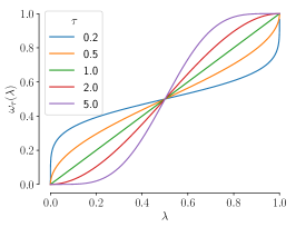
Figure 2: Behavior of $\omega_{\tau}$ for different values of $\tau$.

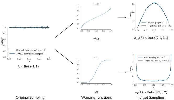
Figure 3: Two examples of coefficients warped to change their underlying distributions. (Left) Original sampling of interpolation coefficients $\lambda$ from $\texttt{Beta}(1,1)$. (Middle) Warping functions $\omega_{0.5}$ (top) and $\omega_{7}$ (bottom) applied. (Right) Resulting distributions of $\omega_{0.5}(\lambda)$ (top) and $\omega_{7}(\lambda)$ (bottom). We can see that $\omega_{0.5}(\lambda)$ closely follows a $\texttt{Beta}(2.1,2.1)$ distribution, and $\omega_{7}(\lambda)$ a $\texttt{Beta}(0.2,0.2)$, respectively shown in blue and black lines in the corresponding plots.

Towards dynamically changing the interpolation depending on the similarity between points, we rely on warping functions $\omega_{\tau}$, to warp interpolation coefficients $\lambda_{t}$ at every iteration $t$ depending on the parameter $\tau$. These functions $\omega_{\tau}$ are bijective transformations from $[0,1]$ to $[0,1]$ defined as such:

$$\omega_{\tau}(\lambda_{t}) =\texttt{BetaCDF}(\lambda_{t};\tau,\tau)$$ (1)

$$=\int_{0}^{\lambda_{t}}\frac{u^{\tau-1}(1-u)^{\tau-1}}{B(\tau,\tau)}du,$$ (2)

where BetaCDF is the cumulative distribution function (CDF) of the Beta distribution, $B(\tau,\tau)$ is a normalization constant and $\tau\in\mathbb{R}^{*}_{+}$ is the warping parameter that governs the strength and direction of the warping. Although the Beta CDF has no closed form solution for non-integer values of its parameters $\alpha$ and $\beta$, accurate approximations are implemented in many statistical software packages. Our motivation behind such $\omega_{\tau}$ is to preserve the same type of distribution after warping, i.e. Beta distributions with symmetry around $0.5$. Similar warping has been used in the Bayesian Optimization literature (Snoek et al., 2014), however many other suitable bijection with sigmoidal shape could be considered in our case. Figure 2 illustrates the shape of $\omega_{\tau}$ and their behavior with respect to $\tau$. These functions have a symmetric behavior around $\tau=1$ (in green), for which warped outputs remain unchanged. When $\tau>1$ (in red and purple) they are pushed towards the extremes ($0$ and $1$), and when $\tau<1$ (in orange and blue), they are pulled towards the center ($0.5$). We further note that the strength of the warping is logarithmic with respect to $\tau$.

Using such warping functions presents the advantage of being able to easily separate the mixing of inputs and targets, by defining different warping parameters $\tau^{(i)}$ and $\tau^{(o)}$. We can now extend the above framework into warped mixup:

$$\tilde{{\mathbf{x}}}_{i} :=\omega_{\tau^{(i)}}(\lambda_{t}){\mathbf{x}}_{i}+(1-\omega_{\tau^{(i)}}(\lambda_{t})){\mathbf{x}}_{\sigma_{t}(i)}$$ (3)

$$\tilde{y}_{i} :=\omega_{\tau^{(o)}}(\lambda_{t})y_{i}+(1-\omega_{\tau^{(o)}}(\lambda_{t}))y_{\sigma_{t}(i)}.$$ (4)

Disentangling inputs and targets can be interesting when working in the imbalanced setting (Chou et al., 2020). Notably, with $\tau^{(i)}=1,\tau^{(o)}\approx+\infty$, we recover the Mixup Input Only (IO) variant (Wang et al., 2023) where only inputs are mixed, and with $\tau^{(i)}\approx+\infty,\tau^{(o)}=1$, the Mixup Target Only (TO) variant (Wang et al., 2023), where only labels are mixed.

Figure 3 presents two examples of warping interpolation coefficients $\lambda$, using two different warping parameters $\tau$ to illustrate the corresponding changes in the underlying distribution of these coefficients. In the following part, we detail our method to select the right $\tau$ depending on the data to mix.

3.3 Similarity-based Kernel Warping

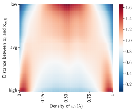
Figure 4: Density of interpolation coefficients after warping with the similarity kernel $\omega_{\tau}(\lambda)$ depending on the distance between pairs $({\mathbf{x}}_{i},{\mathbf{x}}_{\sigma(i)})$ to mix. Close distances (top lines of the heatmap) induce strong interpolations, while far distances (bottom lines of the heatmap) reduce interpolation.

Recall that our goal is to apply stronger interpolation between similar points, and reduce interpolation otherwise, using the warping functions $\omega_{\tau}$ defined above. Therefore, the parameter $\tau$ should be exponentially correlated with the distance, with a symmetric behavior around 1. To this end, we define a class of similarity kernels, based on an inversed, normalized and centered Gaussian kernel, that outputs the correct warping parameter for the given pair of points. Given a batch of data ${\mathbf{x}}=\{{\mathbf{x}}_{i}\}_{i=1}^{n}\in\mathbb{R}^{d\times n}$, the index of the first element in the mix $i\in\{1,\dots,n\}$, along with the permutation $\sigma\in\mathfrak{S}_{n}$ to obtain the index of the second element, we compute the following similarity kernel:

$$\tau({\mathbf{x}},i,\sigma;\tau_{\text{max}},\tau_{\text{std}}) =\frac{1}{\tau_{\text{max}}}\exp\left(\frac{\bar{d}({\mathbf{x}}_{i},{\mathbf{x}}_{\sigma(i)})-1}{2\tau_{\text{std}}^{2}}\right),$$ (5)

$$\text{with}\quad\bar{d}({\mathbf{x}}_{i},{\mathbf{x}}_{\sigma(i)}) =\frac{\sum_{k=1}^{d}(x_{(k,i)}-x_{(k,\sigma(i))})^{2}}{\frac{1}{n}\sum_{j=1}^{n}\sum_{k=1}^{d}(x_{(k,j)}-x_{(k,\sigma(j))})^{2}},$$ (6)

where $\bar{d}$ is the squared $L_{2}$ distance divided by the mean distance over the batch, and $\tau_{\text{max}},\tau_{\text{std}}$ are respectively the amplitude and standard deviation (std) of the Gaussian, which are hyperparameters of the similarity kernel. The amplitude $\tau_{\text{max}}$ governs the strength of the interpolation in average, and $\tau_{\text{std}}$ the extent of mixing. Our motivation behind this kernel is to have small values of $\tau$ for small distances and high $\tau$ otherwise, while being able to shut down the mixing effect for points that are too far apart. Figure 4 illustrates the evolution of the density of warped interpolation coefficients $\omega_{\tau}(\lambda)$, depending on the distance between the points to mix. Using this similarity kernel to find the correct $\tau$ to parameterize the warping functions $\omega_{\tau}$ defines our full Kernel Warping Mixup framework. A detailed algorithm of the training procedure can be found in Appendix D.

Note that this exact form of similarity kernel is defined for the warping functions $\omega_{\tau}$ discussed above and used in the experiments in the next section. Other warping functions might require different kernels depending on their behavior with respect to $\tau$. Likewise, we could consider other similarity measures instead of the squared $L_{2}$, such as a cosine similarity or an optimal transport metric.

4 Experiments

We focus our experiments on two very different sets of tasks, namely Image Classification and Regression on Time Series and tabular data. A presentation of the different calibration metrics used can be found in Appendix A.
Image Classification . We mainly follow experimental settings from previous works (Pinto et al., 2022; Wang et al., 2023) and evaluate our approach on CIFAR-10 (C10) and CIFAR-100 (C100) datasets (Krizhevsky et al., 2009) using Resnet34 and Resnet50 architectures (He et al., 2016). For all our experiments, we use SGD as the optimizer with a momentum of $0.9$ and weight decay of $10^{-4}$, a batch size of $128$, and the standard augmentations random crop, horizontal flip and normalization. Models are trained for 200 epochs, with an initial learning rate of $0.1$ divided by a factor $10$ after $100$ and $150$ epochs. We evaluate calibration using ECE (Naeini et al., 2015; Guo et al., 2017), negative log likelihood (NLL) (Hastie et al., 2009) and Brier score (Brier, 1950), after finding the optimal temperature through Temperature Scaling (Guo et al., 2017). Results are reproduced and averaged over 4 different random runs, and we report standard deviation between the runs. For each run, we additionally average the results of the last 10 epochs following (Wang et al., 2023).
Regression . Here again, we mainly follow settings of previous work on regression (Yao et al., 2022a). We evaluate performance on Airfoil (Kooperberg, 1997), Exchange-Rate and Electricity (Lai et al., 2018) datasets using Root Mean Square Error (RMSE) and Mean Averaged Percentage Error (MAPE), along with Uncertainty Calibration Error (UCE) (Laves et al., 2020) and Expected Normalized Calibration Error (ENCE) (Levi et al., 2022) for calibration. We train a three-layer fully connected network augmented with Dropout (Srivastava et al., 2014) on Airfoil, and LST-Attn (Lai et al., 2018) on Exchange-Rate and Electricity. All models are trained for 100 epochs with the Adam optimizer (Kingma & Ba, 2014), with a batch size of 16 and learning rate of $0.01$ on Airfoil, and a batch size of $128$ and learning rate of $0.001$ on Exchange-Rate and Electricity. To estimate variance for calibration, we rely on MC Dropout (Gal & Ghahramani, 2016) with a dropout of $0.2$ and $50$ samples. Results are reproduced and averaged over 5 different random runs for Exchange Rate and Electricity, and over 10 runs for Airfoil. We also report standard deviation between the runs.

4.1 Classification

Figure 5: Heatmaps of Accuracy (left) and ECE (right) from cross validation on C100 for Resnet50.

Table 1: Comparative study on similarity used for Resnet50 on CIFAR10.

Input similarity	Output similarity	($(\tau^{(i)}_{\text{max}},\tau^{(i)}_{\text{std}})$)	($(\tau^{(o)}_{\text{max}},\tau^{(o)}_{\text{std}})$)	Accuracy ($\uparrow$)	ECE ($\downarrow$)	Brier ($\downarrow$)	NLL ($\downarrow$)
Inputs	Inputs	(2,1)	(2,1)	95.73 $\pm$ 0.07	0.77 $\pm$ 0.07	6.91 $\pm$ 0.16	17.06 $\pm$ 0.47
Embedding	Embedding	(2,1)	(2,1)	95.82 $\pm$ 0.04	0.65 $\pm$ 0.09	6.86 $\pm$ 0.05	17.05 $\pm$ 0.3
Classif. weights	Classif. weights	(5,0.75)	(5,0.75)	95.68 $\pm$ 0.07	0.84 $\pm$ 0.1	6.96 $\pm$ 0.11	17.29 $\pm$ 0.31
Embedding	Classif. weights	(2,1)	(2,1.25)	95.79 $\pm$ 0.18	0.66 $\pm$ 0.03	6.89 $\pm$ 0.23	17.29 $\pm$ 0.31
Inputs	Embedding	(2,1)	(2,1)	95.68 $\pm$ 0.12	0.88 $\pm$ 0.11	6.97 $\pm$ 0.17	16.95 $\pm$ 0.39

To find the optimal pair of parameters $(\tau_{\text{max}},\tau_{\text{std}})$, we conducted cross-validation separately on C10 and C100 datasets. We provide heatmaps of the experiments in Figure 5 for C100, and refer to Appendix C for C10. We can clearly see frontiers and regions of the search spaces that are more optimal than others. In particular, high amplitude and std increase accuracy for both datasets, showing the importance of strong interpolation and not being restrictive in the points to mix. However, while calibration is best when $\tau_{\text{std}}$ is low for C10, good calibration requires that $\tau_{\text{max}}$ and $\tau_{\text{std}}$ are both high for C100. This might reflect the difference in terms of number of class and their separability between both datasets, but a deeper study of the behavior of the confidence would be required.

The flexibility in the framework presented allows to measure similarity between points in any space that can represent them, and also disentangle the similarity used for input and targets. For our experiments in classification, we considered different possible choice:
(1) Input distance: we compute the distance between raw input data, i.e. $\bar{d}({\mathbf{x}}_{i},{\mathbf{x}}_{\sigma(i)})$;
(2) Embedding distance: we compute the distance between embeddings of the input data obtained by the encoder at the current training step, i.e. $\bar{d}(h_{\varphi}({\mathbf{x}}_{i}),h_{\varphi}({\mathbf{x}}_{\sigma(i)}))$;
(3) Classification distance: we compute the distance between the classification weights at the current training step of the class corresponding to the input data, i.e. $\bar{d}({\mathbf{w}}_{y_{i}},{\mathbf{w}}_{y_{\sigma(i)}})$;
In Table 1, we compared results for each of these choice and for different combinations of similarity between inputs and targets. We conducted cross-validation in each case to find the best pairs of parameters $(\tau^{(i)}_{\text{max}},\tau^{(i)}_{\text{std}})$ for input similarity and $(\tau^{(o)}_{\text{max}},\tau^{(o)}_{\text{std}})$ for output similarity. We found that results are robust to the choice of similarity considered as difference in performance and calibration are small between them, but using embedding distance for both inputs and targets seems to yield the best results. This is the setting chosen for the remaining experiments in classification.

Table 2: Performance (Accuracy in %) and calibration (ECE, Brier, NLL) comparison with Resnet34. Best in bold, second best underlined.

Dataset	Methods	$\alpha$	Accuracy ($\uparrow$)	ECE ($\downarrow$)	Brier ($\downarrow$)	NLL ($\downarrow$)
C10	ERM Baseline	–	94.69 $\pm$ 0.27	0.82 $\pm$ 0.11	8.07 $\pm$ 0.31	17.50 $\pm$ 0.61
	Mixup	1	95.97 $\pm$ 0.27	1.36 $\pm$ 0.13	6.53 $\pm$ 0.36	16.35 $\pm$ 0.72
		0.5	95.71 $\pm$ 0.26	1.33 $\pm$ 0.08	7.03 $\pm$ 0.46	17.47 $\pm$ 1.18
		0.1	95.37 $\pm$ 0.22	1.13 $\pm$ 0.11	7.37 $\pm$ 0.36	17.43 $\pm$ 0.79
	Mixup IO	1	95.16 $\pm$ 0.22	0.6 $\pm$ 0.11	7.3 $\pm$ 0.33	15.56 $\pm$ 0.67
		0.5	95.31 $\pm$ 0.17	0.58 $\pm$ 0.06	7.12 $\pm$ 0.21	15.09 $\pm$ 0.45
		0.1	95.12 $\pm$ 0.21	0.7 $\pm$ 0.09	7.38 $\pm$ 0.27	15.76 $\pm$ 0.55
	RegMixup	20	96.51 $\pm$ 0.2	0.76 $\pm$ 0.08	5.78 $\pm$ 0.26	13.14 $\pm$ 0.47
	MIT-A ($\Delta\lambda>0.5$)	1	95.78 $\pm$ 0.22	1.02 $\pm$ 0.19	6.51 $\pm$ 0.29	14.04 $\pm$ 0.67
	MIT-L ($\Delta\lambda>0.5$)	1	95.71 $\pm$ 0.06	0.67 $\pm$ 0.12	6.57 $\pm$ 0.12	13.89 $\pm$ 0.28
	Kernel Warping Mixup (Ours)	1	96.16 $\pm$ 0.09	0.51 $\pm$ 0.07	6.39 $\pm$ 0.16	16.59 $\pm$ 0.55
C100	ERM Baseline	–	73.47 $\pm$ 1.59	2.54 $\pm$ 0.15	36.47 $\pm$ 2.05	100.82 $\pm$ 6.93
	Mixup	1	78.11 $\pm$ 0.57	2.49 $\pm$ 0.19	31.06 $\pm$ 0.69	87.94 $\pm$ 1.98
		0.5	77.14 $\pm$ 0.67	2.7 $\pm$ 0.36	32.01 $\pm$ 0.93	91.22 $\pm$ 3.05
		0.1	76.01 $\pm$ 0.62	2.54 $\pm$ 0.24	33.41 $\pm$ 0.57	93.96 $\pm$ 1.76
	Mixup IO	1	74.44 $\pm$ 0.49	2.02 $\pm$ 0.14	35.25 $\pm$ 0.43	96.5 $\pm$ 1.62
		0.5	74.45 $\pm$ 0.6	1.94 $\pm$ 0.09	35.2 $\pm$ 0.58	96.75 $\pm$ 1.89
		0.1	74.21 $\pm$ 0.46	2.39 $\pm$ 0.11	35.38 $\pm$ 0.48	98.24 $\pm$ 1.81
	RegMixup	10	78.49 $\pm$ 0.35	1.64 $\pm$ 0.14	30.42 $\pm$ 0.26	82.20 $\pm$ 0.78
	MIT-A ($\Delta\lambda>0.5$)	1	77.39 $\pm$ 0.32	2.38 $\pm$ 0.14	31.37 $\pm$ 0.46	83.08 $\pm$ 1.38
	MIT-L ($\Delta\lambda>0.5$)	1	76.51 $\pm$ 0.33	2.54 $\pm$ 0.16	32.62 $\pm$ 0.28	86.81 $\pm$ 0.89
	Kernel Warping Mixup (Ours)	1	79.13 $\pm$ 0.44	1.75 $\pm$ 0.44	29.59 $\pm$ 0.52	82.88 $\pm$ 1.32

Table 3: Performance (Accuracy in %) and calibration (ECE, Brier, NLL) comparison with Resnet50. Best in bold, second best underlined.

Dataset	Methods	$\alpha$	Accuracy ($\uparrow$)	ECE ($\downarrow$)	Brier ($\downarrow$)	NLL ($\downarrow$)
C10	ERM Baseline	–	94.26 $\pm$ 0.12	0.56 $\pm$ 0.05	8.56 $\pm$ 0.23	17.93 $\pm$ 0.36
	Mixup	1	95.6 $\pm$ 0.17	1.40 $\pm$ 0.12	7.13 $\pm$ 0.31	17.32 $\pm$ 0.88
		0.5	95.53 $\pm$ 0.18	1.29 $\pm$ 0.15	7.22 $\pm$ 0.30	17.44 $\pm$ 0.66
		0.1	94.98 $\pm$ 0.25	1.29 $\pm$ 0.21	7.83 $\pm$ 0.37	17.84 $\pm$ 0.78
	Mixup IO	1	94.74 $\pm$ 0.34	0.47 $\pm$ 0.07	7.78 $\pm$ 0.41	16.13 $\pm$ 0.75
		0.5	95.07 $\pm$ 0.17	0.48 $\pm$ 0.08	7.39 $\pm$ 0.14	15.23 $\pm$ 0.34
		0.1	94.79 $\pm$ 0.06	0.7 $\pm$ 0.16	7.85 $\pm$ 0.20	16.37 $\pm$ 0.61
	RegMixup	20	96.14 $\pm$ 0.15	0.91 $\pm$ 0.06	6.41 $\pm$ 0.23	14.77 $\pm$ 0.33
	MIT-A ($\Delta\lambda>0.5$)	1	95.68 $\pm$ 0.28	0.88 $\pm$ 0.19	6.58 $\pm$ 0.43	13.88 $\pm$ 0.83
	MIT-L ($\Delta\lambda>0.5$)	1	95.42 $\pm$ 0.14	0.66 $\pm$ 0.08	6.85 $\pm$ 0.18	14.41 $\pm$ 0.32
	Kernel Warping Mixup (Ours)	1	95.82 $\pm$ 0.04	0.65 $\pm$ 0.09	6.86 $\pm$ 0.05	17.05 $\pm$ 0.3
C100	ERM Baseline	–	73.83 $\pm$ 0.82	2.20 $\pm$ 0.13	35.90 $\pm$ 1.04	96.39 $\pm$ 3.45
	Mixup	1	78.05 $\pm$ 0.23	2.41 $\pm$ 0.23	31.26 $\pm$ 0.26	88.01 $\pm$ 0.53
		0.5	78.51 $\pm$ 0.37	2.55 $\pm$ 0.22	30.44 $\pm$ 0.44	85.57 $\pm$ 1.88
		0.1	76.49 $\pm$ 0.86	2.69 $\pm$ 0.13	32.75 $\pm$ 1.05	89.82 $\pm$ 3.87
	Mixup IO	1	75.25 $\pm$ 0.72	1.77 $\pm$ 0.13	34.24 $\pm$ 0.68	91.41 $\pm$ 2.18
		0.5	76.42 $\pm$ 0.81	1.94 $\pm$ 0.15	32.65 $\pm$ 1.01	86.1 $\pm$ 3.04
		0.1	75.82 $\pm$ 0.98	2.1 $\pm$ 0.22	33.45 $\pm$ 1.26	89.54 $\pm$ 3.75
	RegMixup	10	78.44 $\pm$ 0.24	2.20 $\pm$ 0.23	30.82 $\pm$ 0.29	83.16 $\pm$ 1.19
	MIT-A ($\Delta\lambda>0.5$)	1	77.81 $\pm$ 0.42	2.19 $\pm$ 0.05	30.84 $\pm$ 0.53	80.49 $\pm$ 1.45
	MIT-L ($\Delta\lambda>0.5$)	1	77.14 $\pm$ 0.71	2.13 $\pm$ 0.17	31.74 $\pm$ 1.11	82.87 $\pm$ 3.24
	Kernel Warping Mixup (Ours)	1	79.62 $\pm$ 0.68	1.84 $\pm$ 0.22	29.18 $\pm$ 0.78	80.46 $\pm$ 2.08

Then, we present an extensive comparison of results on both C10 and C100 for Resnet34 and Resnet50 respectively in Tables 2 and 3. We compare our Kernel Warping Mixup with Mixup (Zhang et al., 2018) and its variant Mixup-IO (Wang et al., 2023), and with the recent RegMixup (Pinto et al., 2022) and MIT (Wang et al., 2023). We can see that our method outperforms in accuracy both Mixup and Mixup IO variants, with better calibration scores in general. It also yields competitive accuracy and calibration with state-of-the-art approaches RegMixup and MIT. In particular, for C100 with Resnet50, it obtains about 1 percentage point (p.p.) higher in accuracy than Mixup, 3 p.p. higher than Mixup-IO, 1.2 p.p. higher than RegMixup and 2 p.p. higher than MIT, while having the best calibration scores in all metric. Exact values of $(\tau_{\text{max}},\tau_{\text{std}})$ used to derive these results are presented in Appendix E.

However, our method achieves its competitive results while being much more efficient than the other state-of-the-art approaches. Indeed, our Kernel Warping Mixup is about as fast as Mixup when using input or classification distance, and about $1.5\times$ slower with embedding distance as we have additional computations to obtain the embeddings. However, both RegMixup and MIT are about $2\times$ slower, along with significant memory constraints, since they require training on twice the amount of data per batch which limits the maximum batch size possible in practice. Exact running time comparison can be seen in Appendix B.

4.2 Regression

Table 4: Performance (RMSE, MAPE) and calibration (UCE, ENCE) comparison on several regression tasks. Best in bold, second best underlined.

Dataset	Methods	$\alpha$	RMSE ($\downarrow$)	MAPE ($\downarrow$)	UCE ($\downarrow$)	ENCE ($\downarrow$)
Airfoil	ERM Baseline	–	2.843 $\pm$ 0.311	1.720 $\pm$ 0.219	107.6 $\pm$ 19.179	0.0210 $\pm$ 0.0078
	Mixup	0.5	3.311 $\pm$ 0.207	2.003 $\pm$ 0.126	147.1 $\pm$ 33.979	0.0212 $\pm$ 0.0063
	Manifold Mixup	0.5	3.230 $\pm$ 0.177	1.964 $\pm$ 0.111	126.0 $\pm$ 15.759	0.0206 $\pm$ 0.0064
	C-Mixup	0.5	2.850 $\pm$ 0.13	1.706 $\pm$ 0.104	111.235 $\pm$ 32.567	0.0190 $\pm$ 0.0075
	Kernel Warping Mixup (Ours)	0.5	2.807 $\pm$ 0.261	1.694 $\pm$ 0.176	126.0 $\pm$ 23.320	0.0180 $\pm$ 0.0047
Exch. Rate	ERM Baseline	–	0.019 $\pm$ 0.0024	1.924 $\pm$ 0.287	0.0082 $\pm$ 0.0028	0.0364 $\pm$ 0.0074
	Mixup	1.5	0.0192 $\pm$ 0.0025	1.926 $\pm$ 0.284	0.0074 $\pm$ 0.0022	0.0352 $\pm$ 0.0059
	Manifold Mixup	1.5	0.0196 $\pm$ 0.0026	2.006 $\pm$ 0.346	0.0086 $\pm$ 0.0029	0.0382 $\pm$ 0.0085
	C-Mixup	1.5	0.0188 $\pm$ 0.0017	1.893 $\pm$ 0.222	0.0078 $\pm$ 0.0020	0.0360 $\pm$ 0.0064
	Kernel Warping Mixup (Ours)	1.5	0.0186 $\pm$ 0.0020	1.872 $\pm$ 0.235	0.0074 $\pm$ 0.0019	0.0346 $\pm$ 0.0050
Electricity	ERM Baseline	–	0.069 $\pm$ 0.003	15.372 $\pm$ 0.474	0.007 $\pm$ 0.001	0.219 $\pm$ 0.020
	Mixup	2	0.071 $\pm$ 0.001	14.978 $\pm$ 0.402	0.006 $\pm$ 0.0004	0.234 $\pm$ 0.012
	Manifold Mixup	2	0.070 $\pm$ 0.001	14.952 $\pm$ 0.475	0.007 $\pm$ 0.0007	0.255 $\pm$ 0.015
	C-Mixup	2	0.068 $\pm$ 0.001	14.716 $\pm$ 0.066	0.007 $\pm$ 0.0006	0.233 $\pm$ 0.015
	Kernel Warping Mixup (Ours)	2	0.068 $\pm$ 0.0006	14.827 $\pm$ 0.293	0.007 $\pm$ 0.001	0.230 $\pm$ 0.013

To demonstrate the flexibility of our framework regarding different tasks, we provide experiments on regression for tabular data and time series. Regression tasks have the advantage of having an obvious meaningful distance between points, which is the label distance. Since we are predicting continuous values, we can directly measure the similarity between two points by the distance between their labels, i.e. $\bar{d}(y_{i},y_{\sigma(i)})$. This avoids the costly computation of embeddings.

In Table 4, we compare our Kernel Warping Mixup with Mixup (Zhang et al., 2018), Manifold Mixup (Verma et al., 2019) and C-Mixup (Yao et al., 2022a). We can see that our approach achieves competitive results with state-of-the-art C-Mixup, in both performance and calibration metrics. Exact values of $(\tau_{\text{max}},\tau_{\text{std}})$ used to derive these results are presented in Appendix E. Notably, unlike C-Mixup, our approach do not rely on sampling rates calculated before training, which add a lot of computational overhead and are difficult to obtain for large datasets. Furthermore, since we only use elements from within the same batch of data, we also reduce memory usage.

5 Conclusion

In this paper, we present Kernel Warping Mixup, a flexible framework for linearly interpolating data during training, based on warping functions parameterized by a similarity kernel. The coefficients governing the interpolation are warped to change their underlying distribution depending on the similarity between the points to mix. This provides an efficient and strong data augmentation approach that can be applied to different tasks by changing the similarity function depending on the application. We show through extensive experiments the effectiveness of the approach to improve both performance and calibration in classification as well as in regression. It is also worth noting that the proposed framework can be extended by combining it with other Mixup variants such as CutMix (Yun et al., 2019) or RegMixup (Pinto et al., 2022). Future works include applications to more complex tasks such as semantic segmentation or monocular depth estimation.

Appendix A Introduction to Calibration Metrics

As discussed in Section 2.2, calibration measures the difference between predictive confidence and actual probability. More formally, with $\hat{y}$ and $y\in{\mathbb{Y}}$, respectively the model’s prediction and target label, and $\hat{p}$ its predicted confidence, a perfectly calibrated model should satisfy $P(\hat{y}=y|\hat{p}=p)=p$, for $p\in[0,1]$.

We use several metrics for calibration in the paper, namely, ECE, Brier score and NLL for classification tasks, and UCE and ENCE for regression tasks. We formally introduce all of them here.

NLL

The negative log-likelihood (NLL) is a common metric for a model’s prediction quality (Hastie et al., 2009). It is equivalent to cross-entropy in multi-class classification. NLL is defined as:

$$\text{NLL}({\mathbf{x}},{\mathbf{y}})=-\frac{1}{N}\sum_{i=1}^{N}\log(\hat{p}({\mathbf{y}}_{i}|{\mathbf{x}}_{i})),$$ (7)

where $\hat{p}({\mathbf{y}}_{i}|{\mathbf{x}}_{i})$ represents the confidence of the model in the output associated to ${\mathbf{x}}_{i}$ for the target class ${\mathbf{y}}_{i}$.

Brier score

The Brier score (Brier, 1950) for multi-class classification is defined as

$$\text{Brier}({\mathbf{x}},{\mathbf{y}})=-\frac{1}{N}\sum_{i=1}^{N}\sum_{j=1}^{c}(\hat{p}(y_{(i,j)}|{\mathbf{x}}_{i})-y_{(i,j)})^{2},$$ (8)

where we assume that the target label ${\mathbf{y}}_{i}$ is represented as a one-hot vector over the $c$ possible class, i.e., ${\mathbf{y}}_{i}\in\mathbb{R}^{c}$. Brier score is the mean square error (MSE) between predicted confidence and target.

ECE

Expected Calibration Error (ECE) is a popular metric for calibration performance for classification tasks in practice. It approximates the difference between accuracy and confidence in expectation by first grouping all the samples into $M$ equally spaced bins $\{B_{m}\}_{m=1}^{M}$ with respect to their confidence scores, then taking a weighted average of the difference between accuracy and confidence for each bin. Formally, ECE is defined as (Guo et al., 2017):

$$\text{ECE}:=\sum_{m=1}^{M}\frac{|B_{m}|}{N}|\text{acc}(B_{m})-\text{conf}(B_{m})|,$$ (9)

with $\text{acc}(B_{m})=\frac{1}{|B_{m}|}\sum_{i\in B_{m}}\mathds{1}_{\hat{y}_{i}=y_{i}}$ the accuracy of bin $B_{m}$, and $\text{conf}(B_{m})=\frac{1}{|B_{m}|}\sum_{i\in B_{m}}\hat{p}({\mathbf{y}}_{i}|{\mathbf{x}}_{i})$ the average confidence within bin $B_{m}$.

A probabilistic regression model takes ${\mathbf{x}}\in{\mathbb{X}}$ as input and outputs a mean $\mu_{y}({\mathbf{x}})$ and a variance $\sigma^{2}_{y}({\mathbf{x}})$ targeting the ground-truth $y\in{\mathbb{Y}}$. The UCE and ENCE calibration metrics are both extension of ECE for regression tasks to evaluate variance calibration. They both apply a binning scheme with $M$ bins over the predicted variance.

UCE

Uncertainty Calibration Error (UCE) (Laves et al., 2020) measures the average of the absolute difference between mean squared error (MSE) and mean variance (MV) within each bin. It is formally defined by

$$\text{UCE}:=\sum_{m=1}^{M}\frac{|B_{m}|}{N}|\text{MSE}(B_{m})-\text{MV}(B_{m})|,$$ (10)

with $\text{MSE}(B_{m})=\frac{1}{|B_{m}|}\sum_{i\in B_{m}}(\mu_{y_{i}}({\mathbf{x}}_{i})-y_{i})^{2}$ and $\text{MV}(B_{m})=\frac{1}{|B_{m}|}\sum_{i\in B_{m}}\sigma^{2}_{y_{i}}({\mathbf{x}}_{i})^{2}$.

ENCE

Expected Normalized Calibration Error (ENCE) (Levi et al., 2022) measures the absolute normalized difference, between root mean squared error (RMSE) and root mean variance (RMV) within each bin. It is formally defined by

$$\text{ENCE}:=\frac{1}{M}\sum_{m=1}^{M}\frac{|\text{RMSE}(B_{m})-\text{RMV}(B_{m})|}{\text{RMV}(B_{m})},$$ (11)

with $\text{RMSE}(B_{m})=\sqrt{\frac{1}{|B_{m}|}\sum_{i\in B_{m}}(\mu_{y_{i}}({\mathbf{x}}_{i})-y_{i})^{2}}$ and $\text{RMV}(B_{m})=\sqrt{\frac{1}{|B_{m}|}\sum_{i\in B_{m}}\sigma^{2}_{y_{i}}({\mathbf{x}}_{i})^{2}}$.

Appendix B Efficiency comparison

Table 5: Training time comparison (in seconds) for a single epoch of CIFAR10 with a Resnet50, measured on a single NVIDIA A100 GPU.

Method	Time per epoch (in s)
Mixup	20
RegMixup	38
MIT-L	40
MIT-A	46
Kernel Warping Mixup - Input	21
Kernel Warping Mixup - Classif.	22
Kernel Warping Mixup - Embedding	28

Table 5 presents comparison of training time for a single epoch on CIFAR10 with a Resnet50. We can see that our Kernel Warping Mixup is about as fast as Mixup when using input or classification distance, and about $1.5\times$ slower with embedding distance as we have additional computations to obtain the embeddings, while both RegMixup and MIT are about $2\times$ slower.

Appendix C Cross Validation Heatmaps

(a) CIFAR10

(b) CIFAR100

Figure 6: Heatmaps of Accuracy (left) and ECE (right) from cross validation on CIFAR10 (top) and CIFAR100 (bottom) for Resnet50.

We provide separate heatmaps of cross-validation for both CIFAR10 and CIFAR100 datasets with Resnet50 in Figure 6, and repeat our observations here. High amplitude and std increase accuracy for both datasets, showing the importance of strong interpolation and not being restrictive in the points to mix. However, while calibration is best when $\tau_{\text{std}}$ is low for C10, good calibration requires that $\tau_{\text{max}}$ and $\tau_{\text{std}}$ are both high for C100. This might reflect the difference in terms of number of class and their separability between both datasets, but a deeper study of the behavior of the confidence would be required.

Appendix D Detailed Algorithm

Input: Batch of data $\mathcal{B}=\{({\mathbf{x}}_{i},y_{i})\}_{i=1}^{n}$, mixup parameter $\alpha$, similarity parameters $(\tau_{\text{max}},\tau_{\text{std}})$, parameters of the model at the current iteration $\theta_{t}$

$\tilde{\mathcal{B}}\leftarrow\varnothing$

$\sigma_{t}\sim\mathfrak{S}_{n}$

  // Sample random permutation

for $\forall i\in\{1,\dots,n\}$ do

       $\lambda_{i}\sim\texttt{Beta}(\alpha,\alpha)$

       // Compute warping parameters for inputs and targets separately through Equations 5 and 6

       $\tau_{i}^{(i)}:=\tau^{(i)}({\mathbf{x}},i,\sigma;\tau_{\text{max}},\tau_{\text{std}})$

       $\tau_{i}^{(o)}:=\tau^{(o)}({\mathbf{x}},i,\sigma;\tau_{\text{max}},\tau_{\text{std}})$

       // Generate new data

       $\tilde{{\mathbf{x}}}_{i}:=\omega_{\tau_{i}^{(i)}}(\lambda_{i}){\mathbf{x}}_{i}+(1-\omega_{\tau_{i}^{(i)}}(\lambda_{i})){\mathbf{x}}_{\sigma(i)}$

       $\tilde{y}_{i}:=\omega_{\tau_{i}^{(o)}}(\lambda_{i})y_{i}+(1-\omega_{\tau_{i}^{(o)}}(\lambda_{i}))y_{\sigma(i)}$

       // Aggregate new batch

       $\tilde{\mathcal{B}}\leftarrow\tilde{\mathcal{B}}\cup(\tilde{{\mathbf{x}}}_{i},\tilde{y}_{i})$

      

Compute and optimize loss over $\tilde{\mathcal{B}}$

Output: updated parameters of the model $\theta_{t+1}$

Algorithm 1 Kernel Warping Mixup training procedure

We present a pseudocode of our Kernel Warping Mixup procedure for a single training iteration in Algorithm 1. The generation of new data is explained in the pseudocode as a sequential process for simplicity and ease of understanding, but the actual implementation is optimized to work in parallel on GPU through vectorized operations.

Appendix E Kernel Warping parameters

Table 6: Parameters of the kernel similarity found through cross-validation for each dataset.

Hyperparameter	Model and Dataset
	Resnet34		Resnet50		Airfoil	Exchange Rate	Electricity
	C10	C100	C10	C100
$\tau_{\text{max}}$	0.5	1	2	2	0.0001	500	0.001
$\tau_{\text{std}}$	1.25	0.75	1	1	1.5	1	1.5

In Table 6, we present the hyperparameters found through cross-validation for each dataset and model. These values were used to obtain the results discussed in Section 4.

References

- Baena et al. (2022) Raphaël Baena, Lucas Drumetz, and Vincent Gripon. A local mixup to prevent manifold intrusion. In 30th European Signal Processing Conference, EUSIPCO 2022, Belgrade, Serbia, August 29 - Sept. 2, 2022, pp. 1372–1376. IEEE, 2022. URL https://ieeexplore.ieee.org/document/9909890.
- Brier (1950) Glenn W Brier. Verification of forecasts expressed in terms of probability. Monthly weather review, 78(1):1–3, 1950.
- Chapelle et al. (2000) Olivier Chapelle, Jason Weston, Léon Bottou, and Vladimir Vapnik. Vicinal risk minimization. In Todd K. Leen, Thomas G. Dietterich, and Volker Tresp (eds.), Advances in Neural Information Processing Systems 13, Papers from Neural Information Processing Systems (NIPS) 2000, Denver, CO, USA, pp. 416–422. MIT Press, 2000. URL https://proceedings.neurips.cc/paper/2000/hash/ba9a56ce0a9bfa26e8ed9e10b2cc8f46-Abstract.html.
- Chawla et al. (2002) Nitesh V Chawla, Kevin W Bowyer, Lawrence O Hall, and W Philip Kegelmeyer. Smote: synthetic minority over-sampling technique. Journal of artificial intelligence research, 16:321–357, 2002.
- Chou et al. (2020) Hsin-Ping Chou, Shih-Chieh Chang, Jia-Yu Pan, Wei Wei, and Da-Cheng Juan. Remix: Rebalanced mixup. In Adrien Bartoli and Andrea Fusiello (eds.), Computer Vision - ECCV 2020 Workshops - Glasgow, UK, August 23-28, 2020, Proceedings, Part VI, volume 12540 of Lecture Notes in Computer Science, pp. 95–110. Springer, 2020. doi: 10.1007/978-3-030-65414-6\_9. URL https://doi.org/10.1007/978-3-030-65414-6_9.
- Chung et al. (2021) Youngseog Chung, Willie Neiswanger, Ian Char, and Jeff Schneider. Beyond pinball loss: Quantile methods for calibrated uncertainty quantification. In M. Ranzato, A. Beygelzimer, Y. Dauphin, P.S. Liang, and J. Wortman Vaughan (eds.), Advances in Neural Information Processing Systems, volume 34, pp. 10971–10984. Curran Associates, Inc., 2021. URL https://proceedings.neurips.cc/paper_files/paper/2021/file/5b168fdba5ee5ea262cc2d4c0b457697-Paper.pdf.
- Dablain et al. (2022) Damien Dablain, Bartosz Krawczyk, and Nitesh V Chawla. Deepsmote: Fusing deep learning and smote for imbalanced data. IEEE Transactions on Neural Networks and Learning Systems, 2022.
- Franchi et al. (2021) Gianni Franchi, Nacim Belkhir, Mai Lan Ha, Yufei Hu, Andrei Bursuc, Volker Blanz, and Angela Yao. Robust semantic segmentation with superpixel-mix. In 32nd British Machine Vision Conference 2021, BMVC 2021, Online, November 22-25, 2021, pp. 158. BMVA Press, 2021. URL https://www.bmvc2021-virtualconference.com/assets/papers/0509.pdf.
- Gal & Ghahramani (2016) Yarin Gal and Zoubin Ghahramani. Dropout as a Bayesian approximation: Representing model uncertainty in deep learning. In Proceedings of the 33rd International Conference on Machine Learning (ICML-16), 2016.
- Greenewald et al. (2021) Kristjan H. Greenewald, Anming Gu, Mikhail Yurochkin, Justin Solomon, and Edward Chien. k-mixup regularization for deep learning via optimal transport. CoRR, abs/2106.02933, 2021. URL https://arxiv.org/abs/2106.02933.
- Guo et al. (2017) Chuan Guo, Geoff Pleiss, Yu Sun, and Kilian Q Weinberger. On calibration of modern neural networks. In International conference on machine learning. PMLR, 2017.
- Guo et al. (2019) Hongyu Guo, Yongyi Mao, and Richong Zhang. Mixup as locally linear out-of-manifold regularization. In Proceedings of the AAAI conference on artificial intelligence, volume 33, pp. 3714–3722, 2019.
- Ha & Bunke (1997) Thien M. Ha and Horst Bunke. Off-line, handwritten numeral recognition by perturbation method. IEEE Trans. Pattern Anal. Mach. Intell., 19(5):535–539, 1997. doi: 10.1109/34.589216. URL https://doi.org/10.1109/34.589216.
- Han et al. (2005) Hui Han, Wen-Yuan Wang, and Bing-Huan Mao. Borderline-smote: a new over-sampling method in imbalanced data sets learning. In International conference on intelligent computing, pp. 878–887. Springer, 2005.
- Hastie et al. (2009) Trevor Hastie, Robert Tibshirani, Jerome H Friedman, and Jerome H Friedman. The elements of statistical learning: data mining, inference, and prediction, volume 2. Springer, 2009.
- He et al. (2008) Haibo He, Yang Bai, Edwardo A Garcia, and Shutao Li. Adasyn: Adaptive synthetic sampling approach for imbalanced learning. In 2008 IEEE international joint conference on neural networks (IEEE world congress on computational intelligence), pp. 1322–1328. Ieee, 2008.
- He et al. (2016) Kaiming He, Xiangyu Zhang, Shaoqing Ren, and Jian Sun. Deep residual learning for image recognition. In 2016 IEEE Conference on Computer Vision and Pattern Recognition, CVPR 2016, Las Vegas, NV, USA, June 27-30, 2016, pp. 770–778. IEEE Computer Society, 2016. doi: 10.1109/CVPR.2016.90. URL https://doi.org/10.1109/CVPR.2016.90.
- Hwang et al. (2022) Inwoo Hwang, Sangjun Lee, Yunhyeok Kwak, Seong Joon Oh, Damien Teney, Jin-Hwa Kim, and Byoung-Tak Zhang. Selecmix: Debiased learning by contradicting-pair sampling. Advances in Neural Information Processing Systems, 35:14345–14357, 2022.
- Inoue (2018) Hiroshi Inoue. Data augmentation by pairing samples for images classification. arXiv preprint arXiv:1801.02929, 2018.
- Islam et al. (2023) Md Amirul Islam, Matthew Kowal, Konstantinos G Derpanis, and Neil DB Bruce. Segmix: Co-occurrence driven mixup for semantic segmentation and adversarial robustness. International Journal of Computer Vision, 131(3):701–716, 2023.
- Kan et al. (2023) Xuan Kan, Zimu Li, Hejie Cui, Yue Yu, Ran Xu, Shaojun Yu, Zilong Zhang, Ying Guo, and Carl Yang. R-mixup: Riemannian mixup for biological networks. In Ambuj Singh, Yizhou Sun, Leman Akoglu, Dimitrios Gunopulos, Xifeng Yan, Ravi Kumar, Fatma Ozcan, and Jieping Ye (eds.), Proceedings of the 29th ACM SIGKDD Conference on Knowledge Discovery and Data Mining, KDD 2023, Long Beach, CA, USA, August 6-10, 2023, pp. 1073–1085. ACM, 2023. doi: 10.1145/3580305.3599483. URL https://doi.org/10.1145/3580305.3599483.
- Kim et al. (2020) Jang-Hyun Kim, Wonho Choo, and Hyun Oh Song. Puzzle mix: Exploiting saliency and local statistics for optimal mixup. In Proceedings of the 37th International Conference on Machine Learning, ICML 2020, 13-18 July 2020, Virtual Event, volume 119 of Proceedings of Machine Learning Research, pp. 5275–5285. PMLR, 2020. URL http://proceedings.mlr.press/v119/kim20b.html.
- Kingma & Ba (2014) Diederik P Kingma and Jimmy Ba. Adam: A method for stochastic optimization. arXiv preprint arXiv:1412.6980, 2014.
- Kooperberg (1997) Charles Kooperberg. Statlib: an archive for statistical software, datasets, and information. The American Statistician, 51(1):98, 1997.
- Krizhevsky et al. (2009) Alex Krizhevsky, Geoffrey Hinton, et al. Learning multiple layers of features from tiny images. 2009.
- Kuleshov et al. (2018) Volodymyr Kuleshov, Nathan Fenner, and Stefano Ermon. Accurate uncertainties for deep learning using calibrated regression. In International conference on machine learning, pp. 2796–2804. PMLR, 2018.
- Lai et al. (2018) Guokun Lai, Wei-Cheng Chang, Yiming Yang, and Hanxiao Liu. Modeling long-and short-term temporal patterns with deep neural networks. In The 41st international ACM SIGIR conference on research & development in information retrieval, pp. 95–104, 2018.
- Lakshminarayanan et al. (2017) Balaji Lakshminarayanan, Alexander Pritzel, and Charles Blundell. Simple and scalable predictive uncertainty estimation using deep ensembles. Advances in neural information processing systems, 30, 2017.
- Laves et al. (2020) Max-Heinrich Laves, Sontje Ihler, Jacob F Fast, Lüder A Kahrs, and Tobias Ortmaier. Well-calibrated regression uncertainty in medical imaging with deep learning. In Medical Imaging with Deep Learning, pp. 393–412. PMLR, 2020.
- Levi et al. (2022) Dan Levi, Liran Gispan, Niv Giladi, and Ethan Fetaya. Evaluating and calibrating uncertainty prediction in regression tasks. Sensors, 22(15):5540, 2022.
- Liu et al. (2022) Zicheng Liu, Siyuan Li, Di Wu, Zihan Liu, Zhiyuan Chen, Lirong Wu, and Stan Z. Li. Automix: Unveiling the power of mixup for stronger classifiers. In Shai Avidan, Gabriel J. Brostow, Moustapha Cissé, Giovanni Maria Farinella, and Tal Hassner (eds.), Computer Vision - ECCV 2022: 17th European Conference, Tel Aviv, Israel, October 23-27, 2022, Proceedings, Part XXIV, volume 13684 of Lecture Notes in Computer Science, pp. 441–458. Springer, 2022. doi: 10.1007/978-3-031-20053-3\_26. URL https://doi.org/10.1007/978-3-031-20053-3_26.
- Meng et al. (2021) Linghui Meng, Jin Xu, Xu Tan, Jindong Wang, Tao Qin, and Bo Xu. Mixspeech: Data augmentation for low-resource automatic speech recognition. In ICASSP 2021-2021 IEEE International Conference on Acoustics, Speech and Signal Processing (ICASSP), pp. 7008–7012. IEEE, 2021.
- Moon et al. (2020) Jooyoung Moon, Jihyo Kim, Younghak Shin, and Sangheum Hwang. Confidence-aware learning for deep neural networks. In Proceedings of the 37th International Conference on Machine Learning, pp. 7034–7044. PMLR, 2020. URL https://proceedings.mlr.press/v119/moon20a.html. ISSN: 2640-3498.
- Naeini et al. (2015) Mahdi Pakdaman Naeini, Gregory Cooper, and Milos Hauskrecht. Obtaining well calibrated probabilities using bayesian binning. In Proceedings of the AAAI conference on artificial intelligence, volume 29, 2015.
- Palakkadavath et al. (2022) Ragja Palakkadavath, Thanh Nguyen-Tang, Sunil Gupta, and Svetha Venkatesh. Improving domain generalization with interpolation robustness. In NeurIPS 2022 Workshop on Distribution Shifts: Connecting Methods and Applications, 2022.
- Pinto et al. (2022) Francesco Pinto, Harry Yang, Ser-Nam Lim, Philip Torr, and Puneet K. Dokania. Regmixup: Mixup as a regularizer can surprisingly improve accuracy and out distribution robustness. In Advances in Neural Information Processing Systems, 2022.
- Ramé et al. (2021) Alexandre Ramé, Rémy Sun, and Matthieu Cord. Mixmo: Mixing multiple inputs for multiple outputs via deep subnetworks. In 2021 IEEE/CVF International Conference on Computer Vision, ICCV 2021, Montreal, QC, Canada, October 10-17, 2021, pp. 803–813. IEEE, 2021. doi: 10.1109/ICCV48922.2021.00086. URL https://doi.org/10.1109/ICCV48922.2021.00086.
- Simard et al. (2002) Patrice Y Simard, Yann A LeCun, John S Denker, and Bernard Victorri. Transformation invariance in pattern recognition—tangent distance and tangent propagation. In Neural networks: tricks of the trade, pp. 239–274. Springer, 2002.
- Snoek et al. (2014) Jasper Snoek, Kevin Swersky, Rich Zemel, and Ryan Adams. Input warping for bayesian optimization of non-stationary functions. In International Conference on Machine Learning, pp. 1674–1682. PMLR, 2014.
- Song et al. (2019) Hao Song, Tom Diethe, Meelis Kull, and Peter Flach. Distribution calibration for regression. In International Conference on Machine Learning, pp. 5897–5906. PMLR, 2019.
- Srivastava et al. (2014) Nitish Srivastava, Geoffrey Hinton, Alex Krizhevsky, Ilya Sutskever, and Ruslan Salakhutdinov. Dropout: a simple way to prevent neural networks from overfitting. The journal of machine learning research, 15(1):1929–1958, 2014.
- Summers & Dinneen (2019) Cecilia Summers and Michael J Dinneen. Improved mixed-example data augmentation. In 2019 IEEE winter conference on applications of computer vision (WACV), pp. 1262–1270. IEEE, 2019.
- Takahashi et al. (2019) Ryo Takahashi, Takashi Matsubara, and Kuniaki Uehara. Data augmentation using random image cropping and patching for deep cnns. IEEE Transactions on Circuits and Systems for Video Technology, 30(9):2917–2931, 2019.
- Teney et al. (2023) Damien Teney, Jindong Wang, and Ehsan Abbasnejad. Selective mixup helps with distribution shifts, but not (only) because of mixup. arXiv preprint arXiv:2305.16817, 2023.
- Thulasidasan et al. (2019) Sunil Thulasidasan, Gopinath Chennupati, Jeff A Bilmes, Tanmoy Bhattacharya, and Sarah Michalak. On mixup training: Improved calibration and predictive uncertainty for deep neural networks. Advances in Neural Information Processing Systems, 32, 2019.
- Tian et al. (2023) Huan Tian, Bo Liu, Tianqing Zhu, Wanlei Zhou, and S Yu Philip. Cifair: Constructing continuous domains of invariant features for image fair classifications. Knowledge-Based Systems, 268:110417, 2023.
- Tokozume et al. (2018) Yuji Tokozume, Yoshitaka Ushiku, and Tatsuya Harada. Between-class learning for image classification. In Proceedings of the IEEE conference on computer vision and pattern recognition, pp. 5486–5494, 2018.
- Vapnik (1998) Vladimir Vapnik. Statistical learning theory. Wiley, 1998. ISBN 978-0-471-03003-4.
- Venkataramanan et al. (2022) Shashanka Venkataramanan, Ewa Kijak, Laurent Amsaleg, and Yannis Avrithis. AlignMixup: Improving representations by interpolating aligned features. In 2022 IEEE/CVF Conference on Computer Vision and Pattern Recognition (CVPR), pp. 19152–19161. IEEE, 2022. ISBN 978-1-66546-946-3. doi: 10.1109/CVPR52688.2022.01858. URL https://ieeexplore.ieee.org/document/9879131/.
- Verma et al. (2019) Vikas Verma, Alex Lamb, Christopher Beckham, Amir Najafi, Ioannis Mitliagkas, David Lopez-Paz, and Yoshua Bengio. Manifold mixup: Better representations by interpolating hidden states. In Kamalika Chaudhuri and Ruslan Salakhutdinov (eds.), Proceedings of the 36th International Conference on Machine Learning, volume 97 of Proceedings of Machine Learning Research, pp. 6438–6447. PMLR, 09–15 Jun 2019. URL https://proceedings.mlr.press/v97/verma19a.html.
- Wang et al. (2023) Deng-Bao Wang, Lanqing Li, Peilin Zhao, Pheng-Ann Heng, and Min-Ling Zhang. On the pitfall of mixup for uncertainty calibration. In Proceedings of the IEEE/CVF Conference on Computer Vision and Pattern Recognition, pp. 7609–7618, 2023.
- Wang et al. (2017) Jason Wang, Luis Perez, et al. The effectiveness of data augmentation in image classification using deep learning. Convolutional Neural Networks Vis. Recognit, 11(2017):1–8, 2017.
- Wen et al. (2021) Yeming Wen, Ghassen Jerfel, Rafael Muller, Michael W Dusenberry, Jasper Snoek, Balaji Lakshminarayanan, and Dustin Tran. Combining ensembles and data augmentation can harm your calibration. In International Conference on Learning Representations, 2021. URL https://openreview.net/forum?id=g11CZSghXyY.
- Wightman et al. (2021) Ross Wightman, Hugo Touvron, and Herve Jegou. Resnet strikes back: An improved training procedure in timm. In NeurIPS 2021 Workshop on ImageNet: Past, Present, and Future, 2021.
- Yaeger et al. (1996) Larry Yaeger, Richard Lyon, and Brandyn Webb. Effective training of a neural network character classifier for word recognition. In M.C. Mozer, M. Jordan, and T. Petsche (eds.), Advances in Neural Information Processing Systems, volume 9. MIT Press, 1996. URL https://proceedings.neurips.cc/paper_files/paper/1996/file/81e5f81db77c596492e6f1a5a792ed53-Paper.pdf.
- Yao et al. (2022a) Huaxiu Yao, Yiping Wang, Linjun Zhang, James Y Zou, and Chelsea Finn. C-mixup: Improving generalization in regression. Advances in Neural Information Processing Systems, 35:3361–3376, 2022a.
- Yao et al. (2022b) Huaxiu Yao, Yu Wang, Sai Li, Linjun Zhang, Weixin Liang, James Zou, and Chelsea Finn. Improving out-of-distribution robustness via selective augmentation. In International Conference on Machine Learning, pp. 25407–25437. PMLR, 2022b.
- Yun et al. (2019) Sangdoo Yun, Dongyoon Han, Sanghyuk Chun, Seong Joon Oh, Youngjoon Yoo, and Junsuk Choe. Cutmix: Regularization strategy to train strong classifiers with localizable features. In 2019 IEEE/CVF International Conference on Computer Vision, ICCV 2019, Seoul, Korea (South), October 27 - November 2, 2019, pp. 6022–6031. IEEE, 2019. doi: 10.1109/ICCV.2019.00612. URL https://doi.org/10.1109/ICCV.2019.00612.
- Zhang et al. (2018) Hongyi Zhang, Moustapha Cisse, Yann N. Dauphin, and David Lopez-Paz. mixup: Beyond empirical risk minimization. In International Conference on Learning Representations, 2018. URL https://openreview.net/forum?id=r1Ddp1-Rb.
- Zhu et al. (2020) Jianchao Zhu, Liangliang Shi, Junchi Yan, and Hongyuan Zha. Automix: Mixup networks for sample interpolation via cooperative barycenter learning. In Computer Vision–ECCV 2020: 16th European Conference, Glasgow, UK, August 23–28, 2020, Proceedings, Part X 16, pp. 633–649. Springer, 2020.