Monotone Generative Modeling via a Gromov-Monge Embedding

Abstract.

Generative Adversarial Networks (GANs) are powerful tools for creating new content, but they face challenges such as sensitivity to starting conditions and mode collapse. To address these issues, we propose a deep generative model that utilizes the Gromov-Monge embedding (GME). It helps identify the low-dimensional structure of the underlying measure of the data and then map it, while preserving its geometry, into a measure in a low-dimensional latent space, which is then optimally transported to the reference measure. We guarantee the preservation of the underlying geometry by the GME and $c$-cyclical monotonicity of the generative map, where $c$ is an intrinsic embedding cost employed by the GME. The latter property is a first step in guaranteeing better robustness to initialization of parameters and mode collapse. Numerical experiments demonstrate the effectiveness of our approach in generating high-quality images, avoiding mode collapse, and exhibiting robustness to different starting conditions.

1. INTRODUCTION

The fundamental task of data generation requires a good approximation of the underlying distribution of the input dataset in order to generate new instances of data that resemble the original ones. A common strategy to accomplish this employs a neural network to form a mapping from a known distribution in a latent space to the generated distribution in the input space. The objective is to ensure that the generated distribution aligns well with the given dataset. Prominent approaches for generative modeling include Generative Adversarial Networks (GANs) [GPAM⁺, 14], Variational Auto-Encoders (VAEs) [KW, 14], normalizing flows [RM, 15], and diffusion models [HJA, 20], among others. GAN-based methods specifically focus on discovering the generative map from a latent space of significantly lower dimension than the input data, while employing a minimax game of a generator and a discriminator. The use of a low-dimensional latent space can enable efficient generation of high-quality examples when the underlying data distribution can be approximated by a sufficiently smooth low-dimensional structure. This assumption is common in addressing many data science problems and referred to as the manifold hypothesis [FMN, 16, PZA⁺, 21].

GAN-based methods are lucid and intuitive due to their simple underlying optimization problem:

(1) $$\min_{G}C(\mu,G_{\#}\nu),$$

where $C$ is a chosen cost function, $\mu$ is the data distribution, $\nu$ denotes a chosen distribution on the latent space (e.g., a Gaussian), $G$ is the generative map, and $G_{\#}\nu$ is the pushforward measure of $\nu$ from the latent space to the data space. In the original GAN formulation the cost function $C$ is the Jensen-Shannon divergence. On the other hand, Wasserstein GAN (WGAN), and its subsequent improved versions [ACB, 17, GAA⁺, 17, PFL, 18, GAW, 18, GHLY, 21] adopt the Wasserstein-1 distance cost, grounded in optimal transport (OT).

While GAN-based methods enjoy widespread popularity, they exhibit notable drawbacks. A significant challenge arises from the considerable sensitivity of the the generated map to initializations of the neural network parameters, which often hinders effective model training. Another remarkable limitation is mode collapse [AGL⁺, 17, AB, 17], wherein the underlying data distribution exhibits multiple modes, yet the algorithm identifies only a subset of these modes. This leads to generated examples that represent only a limited portion of the dataset. Another source of potential limitation of GAN-based approaches lies in the fact that the formulation in (1) involves two typically high-dimensional measures $\mu$ and $G_{\#}\nu$. To exemplify the problem, we assume that the cost $C$ in (1) is the Wasserstein distance. In this case, the worst-case sample complexity of (1) is of order $O(n^{-2/D})$, where $D$ is the dimension of the data space and $n$ is the number of data points [CRL⁺, 20].

To address these challenges, we carefully design an improved GAN-based method that enjoys interesting theoretical properties. Indeed, most other methods do not impose special regularity properties of the generative map $G$. We guarantee that $G$ of our method is $c$-cyclically monotone, where $c$ is an inherent cost function. Such a property is natural in the theory of optimal mass transport and helps with being more stable to initialization of parameters and with overcoming mode collapse. Indeed, we demonstrate the effectiveness of such monotonicity in an artificial example, where the ground truth information is known and some geometric properties can be easily visualized.

The design of a “monotone-like” generative map is closely linked with a carefully-designed embedding $T$ of the high-dimensional data into the latent space. This process aims to preserve the inherent geometry of the data. Using this embedding we then optimize an optimal-mass-transport distance between $\nu$ and $T_{\#}\mu$, that is, the pushforward of $\mu$ by the latter embedding. To show that the mapping indeed preserves the geometry, we guarantee that under special assumptions it satisfies the bi-Lipschitz property for points in the support of the underlying data distribution that are sufficiently separated from each other. This geometric property leads to a more computationally tractable formulation.

In order to obtain such a geometric property, we employ the Gromov-Wasserstein (GW) distance [Mém, 07], which is known to measure structural discrepancy between distributions in different metric spaces. More precisely, we employ a Gromov-Monge (GM) formulation of this original distance, which replaces the transport plan with an explicit transport map. Our Gromov-Monge embedding (GME) can be obtained by any local minimizer of this distance (using two specified measures). While the GM formulation may not be well-posed (the minimum may not be obtained), our formulation for obtaining the GME is well-posed.

In addition to the carefully developed theory, we demonstrate a simple algorithm that can be viewed as a variant of WGAN with careful regularization terms that incorporate geometric constraints. Our numerical results on both artificial and real datasets demonstrate the competitive performance of our proposed method.

1.1. Related Works

We review works related to ours that involve the Wasserstein-2 ($W_{2}$) distance in GAN-based methods, GW distance, and dimension reduction.

Generative models via $\mathbf{W_{2}}$:

MTOL [20], TJ [19], LSC⁺ [19], KEA⁺ [21], RKB [22] have integrated the $W_{2}$ distance within GAN-based methods. Our approach also employs the $W_{2}$ distance, however, we compute the distance in the latent space. The idea of employing the Wasserstein distance in the latent space has been earlier explored by KEA⁺ [21]. However, their use of Input Convex Neural Networks (ICNN) to parameterize the potential function reveals scalability limitations and poses challenges regarding expressiveness [KLG⁺, 21, RKB, 22].

GW distance:

This distance has been extensively used in quantifying structural differences between diverse distributions, leading to its application in numerous contexts [Mém, 11, PCS, 16, AMJ, 18, XLC, 19, XLZD, 19, LQZ⁺, 22]. It has also been adopted in specific neural network architectures, such as transformers [HZZ, 22]. The application of the GW distance in generative modeling has been limited, with only a handful of generative models utilizing it [BAMKJ, 19, TFC⁺, 19, NTOH, 23]. These existing methods are hampered by computational inefficiencies and may yield undesired results due to the non-convex formulation. In contrast, our model relies on an explicit transport map, offering simplicity, explainability, and enhanced optimization efficiency.

Embedding and dimension reduction:

These play a crucial role in representation learning. While embedding methods such as t-SNE [VdMH, 08] and UMAP [MHM, 18] are primarily designed for visualization, other methods, such as the principal component analysis (PCA) and manifold learning [GCKG, 23], focus on learning effective representations for downstream tasks. Autoencoders are widely regarded as a nonlinear generalization of PCA [GBC, 16, Ch. 2] designed to learn non-linear low-dimensional embeddings. Recent developments of autoencoders have introduced additional constraints to preserve data structures. For instance, KZSN [20], GAL [20], LYSP [22] imposed isometry conditions. However, unlike our use of GM embeddings which consider global distances between all pairs of data points, their definitions of isometries are based on local distortions.

1.2. Contribution

We summarize the main contributions of our work.

1. We derive a novel generative algorithm and prove its generator is $c$-cyclically monotone.

2. This algorithm employs the Gromov-Monge formulation to embed the high-dimensional data into a Euclidean latent space. We prove that the resulting embedding preserves geometric properties of the data.

3. We develop a simple numerical implementation of these ideas that conform with the basic WGAN structure, but with additional regularizations.

4. Numerical experiments on the CIFAR-10 and Celeb-A datasets demonstrate generated images of the highest quality among GAN-based methods and the strongest resilience to mode collapse for CIFAR-10. For a synthetic setting, we illustrate the monotonicity of the generator and the robustness to mode collapse and parameter initialization.

2. OT AND GROMOV-TYPE COSTS

OT has been widely used in machine learning to measure distances or similarities between probability distributions defined on Euclidean spaces. Its underlying mechanism enables transforming one distribution into another one with the lowest possible cost. The Gromov-Wasserstein formalism, which was initiated by Mém [07], generalizes the OT strategy to probability distributions on possibly different metric spaces. We first review the formulation of OT, followed by an overview of GW. We remark that throughout the paper we assume that any cost function $c$ is continuous.

Throughout the rest of the paper we assume subsets ${X}\subset\mathbb{R}^{D}$ and ${Y}\subset\mathbb{R}^{d}$, where $D>d$, probability measures $\mu\in\mathcal{P}({X})$ and $\nu\in\mathcal{P}({Y})$, and a chosen cost function $c:{X}\times{Y}\rightarrow\mathbb{R}$. The OT cost between $\mu$ and $\nu$ takes the form

(2) $$\operatorname{OT}_{c}(\mu,\nu):=\inf_{\pi\in\Pi(\mu,\nu)}\mathop{\operatorname{\mathop{\mathbb{E}}}}_{(x,y)\sim\pi}[c(x,y)],$$

where $\Pi(\mu,\nu)$ is the following set of transport plans with respective marginals $\mu$ and $\nu$:

$$\Pi(\mu,\nu):=\big{\{}\pi\in\mathcal{P}({X}\times{Y}):\pi(A\times{Y})=\mu(A),\pi({X}\times B)=\nu(B)\ \ \forall\,A\subset{X},B\subset{Y}\big{\}}.$$

If ${D}={d}$, $p\in[1,\infty)$ and $c(x,y)=\|x-y\|^{p}$, then $\sqrt[p]{\operatorname{OT}(\mu,\nu)}$ is the Wasserstein-p distance.

If $\mu$ is absolutely continuous, then the OT cost can be expressed as follows using the transport map $T:{X}\rightarrow{Y}$ [San, 15] and its pushforward measure, $T_{\#}\mu$, which is defined as $T_{\#}\mu(A)=\mu(T^{-1}(A))$ for any Borel measurable $A\subset{X}$:

(3) $$\operatorname{OT}_{c}(\mu,\nu)=\inf_{T_{\#}\mu=\nu}\mathop{\operatorname{\mathop{\mathbb{E}}}}_{x\sim\mu}[c(x,T(x))].$$

The GW cost is a variant of the OT cost which applies to two measures from heterogeneous metric spaces. Given two probability measures $\mu$ and $\nu$ defined on the metric spaces $X$ and $Y$, respectively, and cost functions $c_{X}:X^{2}\to\mathbb{R}$ and $c_{Y}:Y^{2}\to\mathbb{R}$, the GW cost, $\operatorname{GW}(\mu,\nu)\equiv\operatorname{GW}_{c_{X},c_{Y}}(\mu,\nu)$, is defined by

(4) $$\operatorname{GW}(\mu,\nu):=\inf_{\pi\in\Pi(\mu,\nu)}\mathop{\operatorname{\mathop{\mathbb{E}}}}_{((x,y),(x^{\prime},y^{\prime}))\sim\pi\times\pi}\left[\left|c_{X}(x,x^{\prime})-c_{Y}(y,y^{\prime})\right|^{2}\right].$$

The GW cost thus finds the coupling between the two metric spaces that minimizes the cost of matching pairs of points from one space to the other, i.e. $(x,x^{\prime})\in{X}^{2}$ and $(y,y^{\prime})\in{Y}^{2}$.

An alternative Gromov-Monge (GM) cost uses a transport map $T:X\rightarrow Y$ instead of the GW cost as follows:

(5) $$\operatorname{GM}(\mu,\nu):=\inf_{T_{\#}\mu=\nu}\mathop{\operatorname{\mathop{\mathbb{E}}}}_{(x,x^{\prime})\sim\mu\times\mu}\left[|c_{X}(x,x^{\prime})-c_{Y}(T(x),T(x^{\prime}))|^{2}\right].$$

In general, $\operatorname{GW}(\mu,\nu)\leq\operatorname{GM}(\mu,\nu)$.

3. EMBEDDING VIA THE GM COST

We introduce an embedding minimization problem, leveraging the GM cost. Specifically, we aim to find a mapping $T$ in the set $\mathrm{Lip}_{L}(\operatorname{\mathop{\mathrm{supp}}}(\mu),Y)$ of $L$-Lipschitz functions from $\operatorname{\mathop{\mathrm{supp}}}(\mu)$ to $Y$, where $\operatorname{\mathop{\mathrm{supp}}}(\mu)$ represents the support of $\mu$ and $L>0$ is fixed, that solves

(6) $$\min_{T\in\mathrm{Lip}_{L}(\operatorname{\mathop{\mathrm{supp}}}(\mu),Y)}\operatorname{GM}(\mu,T_{\#}\mu).$$

We remark that we eventually approximate $T$ by a neural network, and thus the assumption of being an $L$-Lipschitz function for some $L>0$ is natural.

There are two key differences between (5) and (6). First, (6) eliminates the constraint $T_{\#}\mu=\nu$, and thus gives rise to an unconstrained nonconvex optimization. Second,  (6) replaces $\inf$ with $\min$. This is possible because $\mathrm{Lip}_{L}(\operatorname{\mathop{\mathrm{supp}}}(\mu),Y)$ is compact and the objective function in (6) is continuous in $T$ and bounded from below by $0$.

We rewrite (6) as $\min\limits_{T\in\mathrm{Lip}_{L}(\operatorname{\mathop{\mathrm{supp}}}(\mu),Y)}\operatorname{GM}(T;\mu)$, where

(7) $$\operatorname{GM}(T;\mu):=\mathop{\operatorname{\mathop{\mathbb{E}}}}_{(x,x^{\prime})\sim\mu\times\mu}\left[|c_{X}(x,x^{\prime})-c_{Y}(T(x),T(x^{\prime}))|^{2}\right].$$

We refer to $\operatorname{GM}(T,\mu)$ as the Gromov-Monge Embedding (GME) cost and to any local minimizer of $\operatorname{GM}(T,\mu)$ solving (6) as a GME.

3.1. A Geometric Property of any GME

We show in this section that the GME preserves the geometric properties of the underlying data distribution. Specifically, we guarantee that under special assumptions it satisfies the bi-Lipschitz property for points in the support of the underlying data distribution that are sufficiently separated. One of these assumptions is that $\operatorname{\mathop{\mathrm{supp}}}(\mu)$ is bi-Lipschitz equivalent to $Y$, which is a nonsmooth instance of the “manifold hypothesis”. We remark that this assumption and our claimed bi-Lipschitz property for well-separated points imply that if $Y=\operatorname{\mathop{\mathrm{supp}}}(\nu)$, then the high-dimensional distances between well-separated points in the support of $\mu$ and $G_{\#}\nu$ are well-approximated by the lower-dimensional distance between $T_{\#}\mu$ and $(T\circ G)_{\#}\nu$. Therefore, this geometric property leads to a more computationally tractable formulation. This property is formulated below in Theorem 3.1. Remark 3.1 then explains how to make the required separating distance as small as needed.

For ease of presentation, we formulate the desired property with the quadratic cost functions $c_{X}(x,x^{\prime})=\|x-x^{\prime}\|^{2}$ and $c_{Y}(y,y^{\prime})=\|y-y^{\prime}\|^{2}$. We extend the theory to other costs useful for us in the appendix.

Theorem 3.1.

Assume there exist $h:\operatorname{\mathop{\mathrm{supp}}}(\mu)\rightarrow Y$ and ${\epsilon}>0$ such that for all $x,x^{\prime}\in\operatorname{\mathop{\mathrm{supp}}}(\mu)$

$$(1-{\epsilon})\|x-x^{\prime}\|^{2}\leq\|h(x)-h(x^{\prime})\|^{2}\leq(1+{\epsilon})\|x-x^{\prime}\|^{2}.$$

Suppose $T\in\mathrm{Lip}_{L}(\operatorname{\mathop{\mathrm{supp}}}(\mu),Y)$, where $L>1/\sqrt{3}$, is a local minimizer of $\operatorname{GM}(T,\mu)$. Let $\delta>0$ such that satisfy $9\delta<L^{2}$ and $\Theta\geq 1$ such that

$$\Theta(\Theta-1)\geq L^{2}\left(\left(\frac{1-\epsilon}{1+\epsilon}\right)\frac{L^{2}-9\delta}{L^{2}-1/3}-1\right).$$

If $z,z^{\prime}\in\operatorname{\mathop{\mathrm{supp}}}(\mu)$ are well-separated as follows: for $K:=B(z,\sqrt{\delta}\|z-z^{\prime}\|/2L)\times B(z^{\prime},\sqrt{\delta}\|z-z^{\prime}\|/2L)$,

(8) $$\int_{K}\|x-x^{\prime}\|^{4}d\mu(x)d\mu(x^{\prime})\geq\left(\frac{1+\epsilon}{1-\epsilon}\right)\left(\frac{L^{2}-1/3}{L^{2}-{9{\delta}}}\right)\int_{X^{2}}\|x-x^{\prime}\|^{4}d\mu(x)d\mu(x^{\prime}),$$

then $T$ satisfies

$$\delta\|z-z^{\prime}\|^{2}\leq\|T(z)-T(z^{\prime})\|^{2}\leq\Theta\|z-z^{\prime}\|^{2}.$$

Remark 3.1.

We can add to $GME(T,\mu)$ the regularization term $\int_{X^{2}}-\gamma\|T(x)-T(x^{\prime})\|^{2}e^{-\|x-x^{\prime}\|^{2}}d\mu d\mu$ in order to relax (8) and require instead the bi-Lipschitz property for $z,z^{\prime}\in\operatorname{\mathop{\mathrm{supp}}}(\mu)$ such that $\|z-z^{\prime}\|>C(\gamma)$ where the constant $C(\gamma)$ can be small enough given a sufficiently large $\gamma$. We verify this in the appendix, where we further require that $\mu$ is absolutely continuous and its density is uniformly bounded below by a positive constant.

4. GENERATION VIA GME

We describe the details of our GAN-based method that utilizes the GME. Section 4.1 first formally develops this idea for continuous measures and establishes the $c$-cyclical monotonicity of the generative map. Section 4.1 describes the details of the corresponding algorithm.

4.1. $\mathbf{c}$-Cyclically Monotone Generative Map

Throughout this subsection we assume that $\mu$ and $\nu$ are absolutely continuous probability measures on $X\subset\mathbb{R}^{D}$ and $Y\subset\mathbb{R}^{d}$, respectively.

For a GME, $T:\operatorname{\mathop{\mathrm{supp}}}(\mu)\rightarrow Y$, we define the cost function $c:X\times Y\rightarrow\mathbb{R}$ as follows: $c(x,y)=\|T(x)-y\|^{2}$. We use it to define the following optimal transport cost between $\mu$ and $\nu$:

$$\operatorname{OT}_{c}(\mu,\nu)=\min_{\pi\in\Pi(\mu,\nu)}\displaystyle\mathop{\operatorname{\mathop{\mathbb{E}}}}_{(x,y)\sim\pi}[\|T(x)-y\|^{2}].$$

Using a change of variable, which is clarified in the appendix, we can rewrite the OT cost as

$$\operatorname{OT}_{c}(\mu,\nu)=\min_{\pi\in\Pi(T_{\#}\mu,\nu)}\displaystyle\mathop{\operatorname{\mathop{\mathbb{E}}}}_{(x,y)\sim\pi}[\|x-y\|^{2}].$$

This OT cost can also be interpreted as the squared Wasserstein-2 distance between $T_{\#}\mu$ and $\nu$. It thus reduces the initial cost in (1) from high dimensions to low dimensions.

Using Brenier’s Theorem [Bre, 87], $\operatorname{OT}_{c}(\mu,\nu)$ can be expressed as follows

(9) $$\min_{\begin{subarray}{c}R:Y\rightarrow Y\\ T_{\#}\mu=R_{\#}\nu\end{subarray}}\displaystyle\mathop{\operatorname{\mathop{\mathbb{E}}}}_{y\sim\nu}[\|R(y)-y\|^{2}].$$

By introducing a dual variable for the constraint, it is equivalent to

$$\min_{R:Y\rightarrow Y}\max_{\phi\in C_{0}(Y,\mathbb{R})}\Big{\{}\displaystyle\mathop{\operatorname{\mathop{\mathbb{E}}}}_{y\sim\nu}[\phi(R(y))]-\displaystyle\mathop{\operatorname{\mathop{\mathbb{E}}}}_{x\sim\mu}[\phi(T(x))]+\displaystyle\mathop{\operatorname{\mathop{\mathbb{E}}}}_{y\sim\nu}[\|R(y)-y\|^{2}]\Big{\}}.$$

If $T$ is invertible, we define the generator $G:=T^{-1}\circ R$ and the discriminator $\psi:=\phi\circ T$ and rewrite the above equation as the following minimax game of $G$ and $\psi$:

(10) $$\min_{G}\max_{\psi}\Big{\{}\displaystyle\mathop{\operatorname{\mathop{\mathbb{E}}}}_{y\sim\nu}[\psi(G(y))]-\displaystyle\mathop{\operatorname{\mathop{\mathbb{E}}}}_{x\sim\mu}[\psi(x)]+\displaystyle\mathop{\operatorname{\mathop{\mathbb{E}}}}_{y\sim\nu}[\|T\circ G(y)-y\|^{2}]\Big{\}}.$$

Figure 1 demonstrates the maps $G$, $T$, and $R$.

Figure 1. Illustration of our basic idea for generation on $X$ with a latent space $Y$ and given data on $X$.

Note that Theorem 3.1 implies that when restricted to sufficiently well-separated points, $T$ is invertible. Moreover, Remark 3.1 clarifies how to make the required separation distance arbitrarily small. Therefore, in the setting of this theorem and having a practical scenario of i.i.d. samples from $\mu$ we can expect $T$ to be invertible and thus $G$ is well-defined. However, to address the most general scenario, we assume for the rest of this section that $T$ is invertible.

The following theorem demonstrates that the composite map $G$ forms a generative map from $\nu$ to $\mu$.

Theorem 4.1 ($G_{\#}\nu=\mu$).

If $\mu\in{\mathcal{P}}(X)$ and $\nu\in{\mathcal{P}}(Y)$ are absolutely continuous, $T$ is an invertible GME for $\mu$ and $R$ is the minimizer of (9), then $G=T^{-1}\circ R$ is a generative map that satisfies $G_{\#}\nu=\mu.$

Next, we establish an important property of $G$, which is based on the following definition [San, 15].

Definition 4.1.

For $c:X\times Y\rightarrow\mathbb{R}$, a set $\Gamma\subset X\times Y$ is $c$-cyclically monotone ($c$-CM) if for every $k\in\mathbb{N}$, every permutation $\sigma$ and every finite family of points $(x_{1},y_{1}),\cdots,(x_{k},y_{k})\in\Gamma$,

$$\sum^{k}_{i=1}c(x_{i},y_{i})\leq\sum^{k}_{i=1}c(x_{\sigma(i)},y_{i}).$$

The following theorem provides evidence of the generative map, denoted as $G$, satisfying $c$-CM property.

Theorem 4.2 ($c$-CM map).

If $\mu\in{\mathcal{P}}(X)$ and $\nu\in{\mathcal{P}}(Y)$ are absolutely continuous, $T$ is an invertible GME for $\mu$, $R:Y\rightarrow Y$ is the minimizer of (9) and $G=T^{-1}\circ R$, then the set $\Gamma=\{(G(y),y)\in X\times Y\}$ is $c$-CM where the cost function $c$ is defined by $c(x,y)=\|T(x)-y\|^{2}$.

4.2. Algorithm

We explain how to approximate $G$ and $\psi$, described in (10), by neural networks (NNs) and consequently describe how to implement the ideas of Section 4.1.

We define the NN functions $G_{{\bm{\theta}}_{1}}$ and $\psi_{{\bm{\theta}}_{2}}=\phi_{{\bm{\theta}}_{4}}\circ T_{{\bm{\theta}}_{3}}$ where $G_{{\bm{\theta}}_{1}}$, $T_{{\bm{\theta}}_{3}}$, and $\phi_{{\bm{\theta}}_{4}}$ approximate $G,T$, and $\phi$, respectively. Here, ${\bm{\theta}}_{1}$, ${\bm{\theta}}_{2}$, ${\bm{\theta}}_{3}$, ${\bm{\theta}}_{4}$ represent vectors of parameters for the respective networks, and ${\bm{\theta}}_{2}=({\bm{\theta}}_{3},{\bm{\theta}}_{4})$.

To motivate our idea for algorithmic implementation, we first assume that $T_{{\bm{\theta}}_{3}}$ was trained beforehand to minimize $\operatorname{GM}(T_{{\bm{\theta}}_{3}},\mu)$. The minimax problem in (10) can then be expressed as

(11) $$\min_{{\bm{\theta}}_{1}}\max_{{\bm{\theta}}_{2}}\Big{\{}\displaystyle\mathop{\operatorname{\mathop{\mathbb{E}}}}_{y\sim\nu}[\psi_{{\bm{\theta}}_{2}}(G_{{\bm{\theta}}_{1}}(y))]-\displaystyle\mathop{\operatorname{\mathop{\mathbb{E}}}}_{x\sim\mu}[\psi_{{\bm{\theta}}_{2}}(x)]+\displaystyle\mathop{\operatorname{\mathop{\mathbb{E}}}}_{y\sim\nu}[\|T_{{\bm{\theta}}_{3}}\circ G_{{\bm{\theta}}_{1}}(y)-y\|^{2}]\Big{\}}.$$

Our implementation uses the following compoents:

$$\mathcal{L}_{1} =\displaystyle\mathop{\operatorname{\mathop{\mathbb{E}}}}_{y\sim\nu}[\psi_{{\bm{\theta}}_{2}}(G_{{\bm{\theta}}_{1}}(y))]-\displaystyle\mathop{\operatorname{\mathop{\mathbb{E}}}}_{x\sim\mu}[\psi_{{\bm{\theta}}_{2}}(x)],$$

$$\mathcal{L}_{2} =\displaystyle\mathop{\operatorname{\mathop{\mathbb{E}}}}_{y\sim\nu}[\|T_{{\bm{\theta}}_{3}}\circ G_{{\bm{\theta}}_{1}}(y)-y\|^{2}],$$

$$\mathcal{L}_{3} =\displaystyle\mathop{\operatorname{\mathop{\mathbb{E}}}}_{x\sim\mu}[\|G_{{\bm{\theta}}_{1}}\circ T_{{\bm{\theta}}_{3}}(x)-x\|^{2}].$$

We note that the loss function in (11) is $\mathcal{L}_{1}+\mathcal{L}_{2}$. Since we consider $\mathcal{L}_{2}$ as a regularization term for enforcing the monotonicity of the generative map, we optimize instead $\mathcal{L}_{1}+\lambda_{2}\mathcal{L}_{2}$. We observed faster convergence speed with smaller $\lambda_{2}$.

We next motivate the above term $\mathcal{L}_{3}$. We first note that $T\circ G=R$ and thus $\mathcal{L}_{2}$ expresses a distance between $\nu$ and $T_{\#}\mu$ so that $R$ is as close as possible to the identity map on the latent space. We further note that $G\circ T=T^{-1}\circ R\circ T$ and that the term $\mathcal{L}_{3}$ expresses a distance between $\nu$ and $T_{\#}\mu$ so that $T^{-1}\circ R\circ T$ is as close as possible to the identity on the ambient space. If we have the bi-Lipschitz assumption of Theorem 3.1 between the support of $\nu$ and $\mu$ and the bi-Lipschitz property of $T$ (practically implied by the theorem), then there is no need to further minimize $\mathcal{L}_{3}$; however, to enforce a geometric-preserving property of $T$ and explore more carefully the possible similarity between the underlying low-dimensional geometries of $\mu$ and $\nu$, we incorporate $\mathcal{L}_{3}$ and thus try to minimize $\mathcal{L}_{1}+\lambda_{2}\mathcal{L}_{2}+\lambda_{3}\mathcal{L}_{3}$.

In this setting, it is natural to iterate the following scheme to solve (11): for $k=1,2,\cdots$,

$${\bm{\theta}}_{1} \leftarrow{\bm{\theta}}_{1}-\alpha_{1}\nabla_{{\bm{\theta}}_{1}}\big{(}\mathcal{L}_{1}+\lambda_{2}\mathcal{L}_{2}+\lambda_{3}\mathcal{L}_{3}\big{)}$$

$${\bm{\theta}}_{2} \leftarrow{\bm{\theta}}_{2}+\alpha_{2}\nabla_{{\bm{\theta}}_{2}}\mathcal{L}_{1}.$$

Here, $\alpha_{1}$ and $\alpha_{2}$ are learning rates, and $\lambda_{1}$, $\lambda_{2}$, and $\lambda_{3}$ are regularization parameters.

In practice, instead of learning $T_{{\bm{\theta}}_{3}}$ separately, we train all the networks in an end-to-end fashion. To achieve this, we simultaneously maximize $T_{{\bm{\theta}}_{3}}$ and $\psi_{{\bm{\theta}}_{2}}$, where we recall that ${\bm{\theta}}_{2}=({\bm{\theta}}_{3},{\bm{\theta}}_{4})$, by adding a GME regularization term, which enforces $T_{{\bm{\theta}}_{3}}$ to minimize $\operatorname{GM}(T_{{\bm{\theta}}_{3}},\mu)$. That is,

(12) $${\bm{\theta}}_{1} \leftarrow{\bm{\theta}}_{1}-\alpha_{1}\nabla_{{\bm{\theta}}_{1}}\big{(}\mathcal{L}_{1}+\lambda_{2}\mathcal{L}_{2}+\lambda_{3}\mathcal{L}_{3}\big{)}$$

(13) $${\bm{\theta}}_{2} \leftarrow{\bm{\theta}}_{2}+\alpha_{2}\nabla_{{\bm{\theta}}_{2}}\big{(}\mathcal{L}_{1}-\lambda_{1}\operatorname{GM}(T_{{\bm{\theta}}_{3}},\mu)\big{)}.$$

The resulting algorithm, which we refer to as the Gromov-Monge Embedding GAN, or GMEGAN, is summarized in Algorithm 1, In Algorithm 1, which uses the following relative error

$$\operatorname{rel.err}({\bm{\theta}}_{1}^{(k)},{\bm{\theta}}_{1}^{(k+1)},{\bm{\theta}}_{2}^{(k)},{\bm{\theta}}_{2}^{(k+1)})=|\mathcal{L}_{1}({\bm{\theta}}_{1}^{(k+1)},{\bm{\theta}}_{2}^{(k+1)})-\mathcal{L}_{1}({\bm{\theta}}_{1}^{(k)},{\bm{\theta}}_{2}^{(k)})|.$$

Input: A dataset $\{x_{i}\}^{n}_{i=1}$ in $X\subset\mathbb{R}^{D}$, a known distribution $\nu\in\mathcal{P}({Y})$, where ${Y}\subset\mathbb{R}^{d}$; functions $c_{X}$, $c_{Y}$; NNs with parameters ${\bm{\theta}}_{1}$ and ${\bm{\theta}}_{2}$ initialized by $({\bm{\theta}}_{1})_{0}$ and $({\bm{\theta}}_{2})_{0}$; parameters $\lambda_{i}$ ($i=1,2,3$) (regularization parameters), $\alpha_{1}$, $\alpha_{2}$ (learning rates), $m\in\mathbb{N}$ (the size of minibatch), $\tau>0$ (tolerance of the iteration)

Output: Generative map $G^{*}_{{\bm{\theta}}_{1}}:Y\rightarrow X$ and a generated distribution $(G^{*}_{{\bm{\theta}}_{1}})_{\#}\nu$

${\bm{\theta}}_{1}^{(0)}=({\bm{\theta}}_{1})_{0}$, ${\bm{\theta}}_{2}^{(0)}=({\bm{\theta}}_{2})_{0}$;

for $k=0,1,2,\cdots$ do

       Sample $\{x_{i}\}^{m}_{i=1}\subset\{x_{i}\}^{n}_{i=1}$ and $\{y_{i}\}^{m}_{i=1}$ from $\nu$;

       Update ${\bm{\theta}}_{1}^{(k+1)}$ using (12);

       Update ${\bm{\theta}}_{2}^{(k+1)}$ using (13);

       if $\operatorname{rel.err}({\bm{\theta}}_{1}^{(k)},{\bm{\theta}}_{1}^{(k+1)},{\bm{\theta}}_{2}^{(k)},{\bm{\theta}}_{2}^{(k+1)})<\tau$ then

             stop the iteration;

            

      

Algorithm 1 Gromov-Monge Embedding GAN (GMEGAN)

5. NUMERICAL EXPERIMENTS

We describe our comprehensive numerical experiments, while leaving some details to the appendix. To ensure a fair comparison, we exclusively evaluate our approach against other GAN-based algorithms and keep the NN architectures identical whenever possible. We omit comparisons with other types of generative models due to the inability to implement exactly the same NN architectures for these methods. Specifically, we compare with GAN [GPAM⁺, 14], Wasserstein GAN (WGAN) [ACB, 17], Wasserstein GAN with gradient penalty (WGP) [GAA⁺, 17], Wasserstein Divergence for GANs (WDIV) [WHT⁺, 18], and OTM [RKB, 22]. We do not include the comparison results for GWGAN [BAMKJ, 19] since it did not converge to a satisfactory FID score under the experimental settings used for comparison.

5.1. Generating Synthetic Gaussian Mixtures

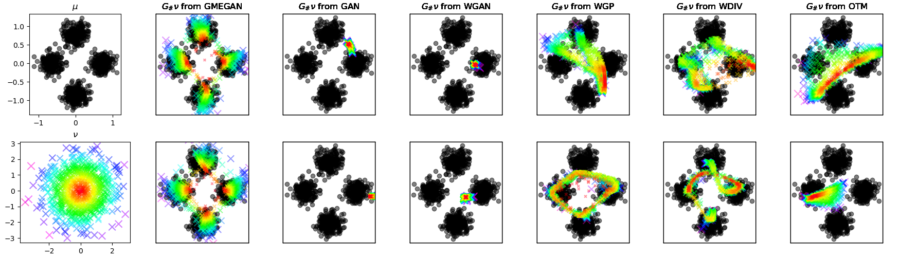
(a) 4 Gaussians

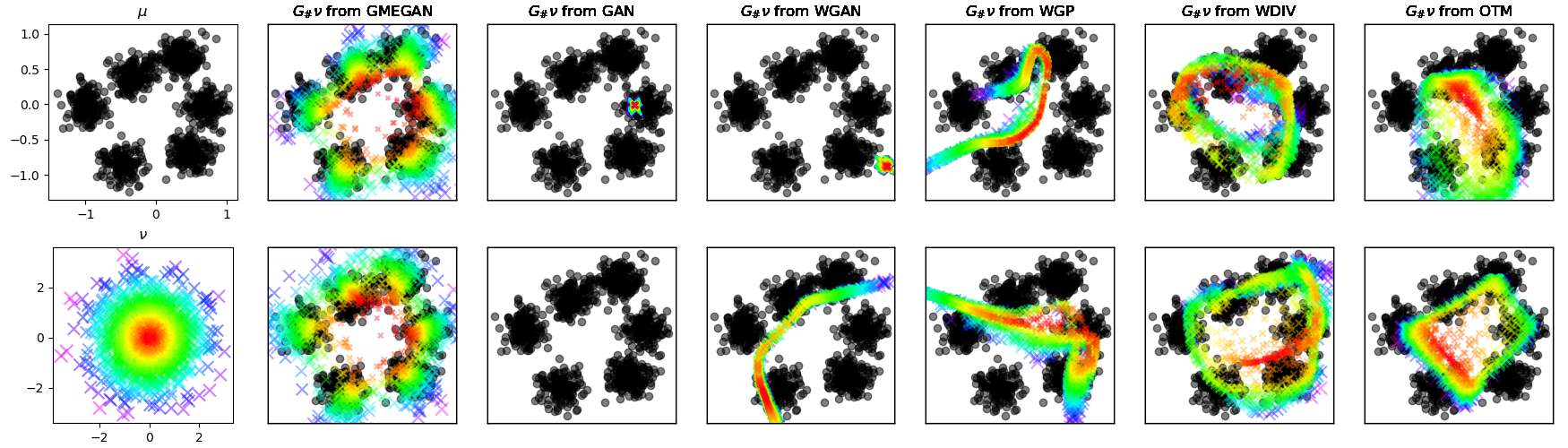
(b) 6 Gaussians

Figure 2. Results for the artificial dataset. The first column illustrates the input dataset in $\mathbb{R}^{50}$ (i.i.d. sampled from a mixture of 4 and 6 Gaussians) and the latent i.i.d. samples from a single Gaussian distribution (colored according to distance from the origin). The remaining columns showcase the generated samples, assigned the original color of the corresponding point in the latent space (for which the generator is applied) and produced by GMEGAN, GAN, WGAN, WGP, WDIV, and OTM. The columns correspond to different parameter initializations.

We consider an artificial dataset that helps us illustrate the concept of monotonicity, existence of mode collapse and sensitivity to parameter initialization. We i.i.d. sample the input dataset $\{x_{i}\}^{n}_{i=1}$, where $n=1,000$, from a mixture of spherical Gaussians in $\mathbb{R}^{50}$ with standard variation 0.15 and with centers located primarily in the first two coordinates. We let the reference distribution $\nu$ be a single spherical Gaussian in $\mathbb{R}^{2}$ and i.i.d. sample $\{y_{i}\}_{i=1}^{m}$, where $m=1,500$, from $\nu$. We train GMEGAN along with the baseline GAN-based methods to learn generative maps from $\mathbb{R}^{2}$ to $\mathbb{R}^{50}$.

Figure 2 demonstrates results for two different choices of the number of Gaussians in the mixture model. The case of 4 Gaussians is demonstrated in Subfigure 2(a)) and that of 6 Gaussians in Subfigure 2(b). In both subfigures, the top image in the first column displays the first two coordinates of $\{x_{i}\}^{n}_{i=1}$ (in black) and the bottom image demonstrates $\{y_{i}\}_{i=1}^{m}$ (in color). The latter color varies according to the distance of each $y_{i}$ from the origin, using the “gist_rainbow” colormap. For clear comparison, we show $\{x_{i}\}^{n}_{i=1}$ (in black) in the other plots of each subfigure. The subsequent columns reveal the first two coordinates of the 1,500 generated samples from the six different GAN-based methods (listed above each column). For a corresponding generator $G:\mathbb{R}^{2}\rightarrow\mathbb{R}^{50}$, these points can be described as $\{G(y_{i})\}_{i=1}^{m}$ and we thus color each generated sample $G(y_{i})$ the same way as $y_{i}$. Each column of each subfigure corresponds to an independent implementation with a randomly chosen parameter initialization.

We observe three key distinctive features of GMEGAN. Firstly, the generated samples by GMEGAN align very well with the input data, unlike the rest of the GAN-based methods. Misalignment with the original data may potentially lead to mode collapse. Indeed, mode collapse is noticed in many of the other images, where severe instances of collapse are observed for GAN and WGAN. Secondly, the color of generated samples by GMEGAN indicate a monotonic behavior, where different colored rings in the bottom left plot of each subfigure are mapped by $G$ of GMEGAN to rings of the same color in the first two coordinates of the high-dimensional space of generation. OTM also seems to display monotonicity, but struggles with generating samples that align well with the input dataset. Other methods do not display any such monotonicity. Finally, the generated samples by GMEGAN in the two different runs are similar, whereas other methods generate different patterns, implying their sensitivity to parameter initialization.

5.2. Generating Real Images

We train GME and the baseline models on two widely used real image datasets, CIFAR-10 [KH⁺, 09] and Celeb-A [LLWT, 15], and compare their performances. For CIFAR-10, we train 300 epochs for each model and illustrate some generated samples in Figure 3. For Celeb-A, we train 100 epochs for each model, except for GAN, whose training diverges at 100 epochs, and we thus only train 90 epochs for GAN. We demonstrate some generated samples in Figure 4.

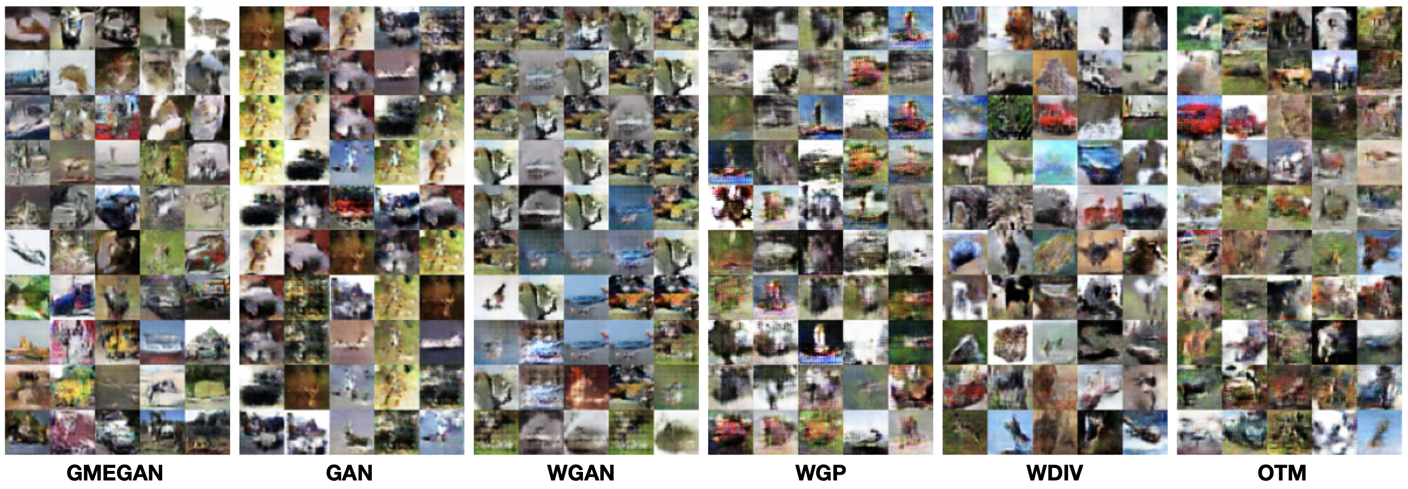
Figure 3. Generated images for CIFAR-10 Dataset at epoch 300.

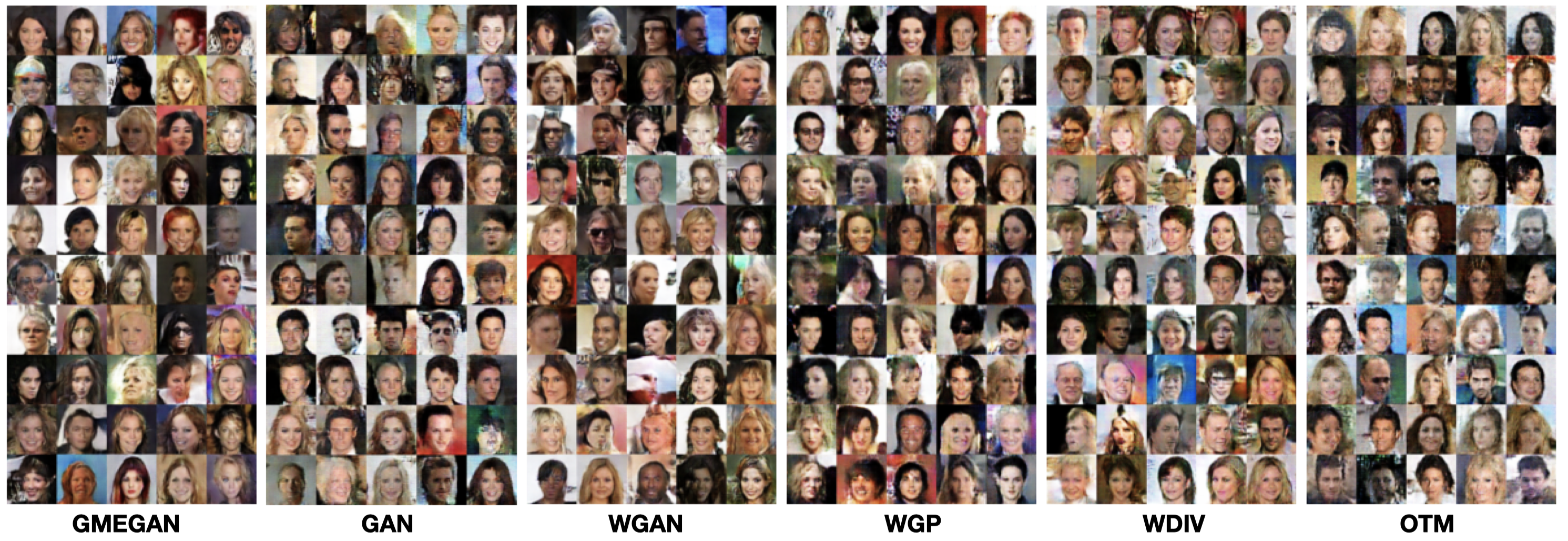
Figure 4. Generated images for Celeb-A Dataset at epoch 100 except GAN which are taken from epoch 90.

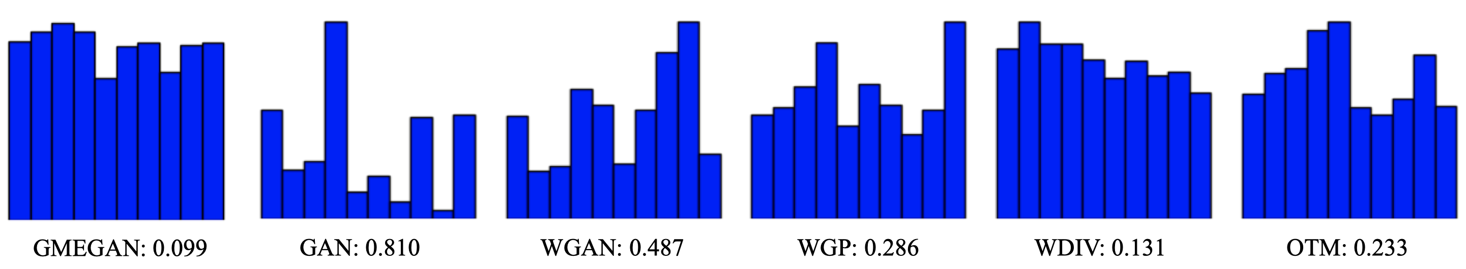
Figure 5. Histograms and relative standard deviations of the generated samples by the different methods. Bars indicate the number of generated points in each of the 10 classes of images.

To compare the quality of the generated images from all the GAN-based methods, we calculate the Fréchet Inception Distance (FID) [HRU⁺, 17] scores between the generated samples and the input dataset. For each method, we calculate means and standard deviations over 40 FID scores, where each FID score is computed using 5,000 randomly sampled real images and 5,000 generated images from the model at epoch 300 for CIFAR-10 and at epoch 100 for Celeb-A. Table 1 presents the FID scores of the six different methods, where a lower FID score indicates superior performance. GMEGAN outperforms the other methods with the lowest FID score on both datasets.

Table 1. Mean and standard deviations of FID scores for CIFAR-10 and Celeb-A (the lower the better)

METHOD	CIFAR-10	CELEB-A
	(EPOCH 300)	(EPOCH 100)
GAN	$56.73\pm 8.67$	$20.61\pm 2.61$
WGAN	$72.16\pm 10.92$	$37.70\pm 13.88$
WGP	$11.73\pm 6.76$	$41.46\pm 6.62$
WDIV	$4.11\pm 0.71$	$43.65\pm 10.48$
OTM	$7.69\pm 2.72$	$31.74\pm 4.37$
GMEGAN	$\mathbf{3.55\pm 0.59}$	$\mathbf{17.02\pm 3.57}$

For CIFAR-10, we employ a quantitative metric for mode collapse, which was proposed by SSM [18]. The idea is to apply a pretrained classifier to assess whether the generated distribution shows mode collapse. For each GAN-based model, we use the classifier to classify 10,000 generated samples. Since CIFAR-10 is composed of 10 equal clusters with the same number of points (6,000), we aim to quantify the uniform distribution among clusters of the generated samples.

Figure 5 demonstrates the histograms obtained by the classifier, i.e., they indicate the number of points per cluster. To further quantify this information, we calculate the relative standard deviation of the number of samples within each class. This relative quantity is the ratio of the standard deviation and the mean. Here, a low relative standard deviation indicates that the generated samples are well-distributed across the ten digits, while a high relative standard deviation suggests the possibility of mode collapse. As the results show, GMEGAN has a relatively flat histogram and the lowest relative standard deviation, demonstrating its robustness against mode collapse.

6. CONCLUSION

We have introduced a GAN-based generative algorithm utilizing both the GME cost and $W_{2}$ distance. Our theoretical analysis shows that local minimizers of the GME cost, which are also Lipschitz, satisfy an approximate bi-Lipschitz property. Using this property, we have proved that the generative map is $c$-cyclically monotone. We also verified that this map pushes forward the reference latent distribution $\nu$ to the data distribution $\mu$.

Numerical experiments demonstrated the monotonicity of the generative map, absence of mode collapse, and robustness to parameter initializations of our method. Using two common benchmarks of image datasets, we further demonstrated the generation of the high-quality images by our method, according to the lowest FID scores, while comparing to other GAN-based methods.

In future work, we intend to broaden the application of the GME cost to various tasks, including but not limited to acquiring Euclidean representations for datasets residing on graphs or manifolds. Furthermore, we aim to formulate regularization strategies to improve tasks beyond generation that utilize the GME cost.

7. ACKNOWLEDGEMENTS

WL acknowledges funding from the National Institute of Standards and Technology (NIST) under award number 70NANB22H021, YY and DZ acknowledge funding from the Kunshan Municipal Government research funding, and GL acknowledges funding from NSF award DMS-2124913.

APPENDIX

We include the following additional information in the supplementary material. Section A contains proofs of the main theoretical results, Section B describes the complete details of our experimental settings, and Section C presents additional results from the experiments.

Appendix A MISSING PROOFS

In this section, we present the detailed proofs of Lemmas and Theorems that are missing in the main paper.

A.1. Proofs of Generalized Versions of Theorem 3.1

In this section, we provide the proof of Theorem 3.1. We actually generalize the theorem to include a modified cost function that includes the following regularization term defined in Remark 3.1: $\int_{X^{2}}-\gamma c_{Y}(T(x),T(x^{\prime}))e^{-\|x-x^{\prime}\|^{2}}d\mu d\mu$. Furthermore, we present theorems for two different types of functions. Specifically, Theorem A.1 pertains for quadratic functions (with $c_{X}(x,x^{\prime})=\|x-x^{\prime}\|^{2}$ and $c_{Y}(y,y^{\prime})=\|y-y^{\prime}\|^{2}$) and Theorem A.2 deals with logarithmic functions (with $c_{X}(x,x^{\prime})=\log(1+\|x-x^{\prime}\|^{2})$ and $c_{Y}(y,y^{\prime})=\log(1+\|y-y^{\prime}\|^{2}))$. We remark that when setting $\gamma=0$ and using the quadratic functions, Theorem A.1 reverts to the statement of Theorem 3.1. In Section B, we will apply these cost functions in experiments involving both artificial and real datasets.

In order to fully formulate the GMT cost for both settings of cost functions, we write in general $c_{X}(x,x^{\prime})=\eta_{X}(x-x^{\prime})$ and $c_{Y}(y,y^{\prime})=\eta_{Y}(y-y^{\prime})$ where $\eta_{X}:X\rightarrow\mathbb{R}$ and $\eta_{Y}:Y\rightarrow\mathbb{R}$ are twice differentiable functions. We can then write the (generalized) GMT cost as

(14) $$\operatorname{GM}(T,\mu)=\int_{X^{2}}|\eta_{X}(x-x^{\prime})-\eta_{Y}(T(x)-T(x^{\prime}))|^{2}-\gamma\eta_{Y}(y-y^{\prime})e^{-\|x-x\|^{2}}d\mu(x)d\mu(x^{\prime}).$$

Theorem A.1.

Let $\mu\in\mathcal{P}(X)$, $c_{X}(x,x^{\prime})=\|x-x^{\prime}\|^{2}$, and $c_{Y}(y,y^{\prime})=\|y-y^{\prime}\|^{2}$. Suppose there exist ${\epsilon}>0$ and $h:\operatorname{\mathop{\mathrm{supp}}}(\mu)\rightarrow Y$ such that

(15) $$(1-{\epsilon})\|x-x^{\prime}\|^{2}\leq\|h(x)-h(x^{\prime})\|^{2}\leq(1+{\epsilon})\|x-x^{\prime}\|^{2}$$

for all $x,y\in\operatorname{\mathop{\mathrm{supp}}}(\mu)$. Suppose $T:\operatorname{\mathop{\mathrm{supp}}}(\mu)\rightarrow Y$ is a $L$-Lipschitz function with $L>1/\sqrt{3}$. Let $\delta$ and $\Theta\geq 1$ be positive constants such that $\delta^{2}<L$ and

(16) $$\left(\Theta^{\prime}(\Theta^{\prime}-1)+L^{2}\right)\Lambda\geq L^{2}\int_{X^{2}}\|x-x^{\prime}\|^{4}d\mu d\mu+\gamma L^{2}\int_{X^{2}}e^{-\|x-x^{\prime}\|^{2}}\|x-x^{\prime}\|^{2}d\mu d\mu$$

where $\Theta^{\prime}=\frac{\Theta-\sqrt{\delta}}{1+\sqrt{\delta}/L}$ and $\Lambda>0$ is defined as

$$\Lambda:=\frac{L^{2}-1/3}{L^{2}-\frac{4{\delta}}{(1-\sqrt{\delta}/L)^{2}}}\left(\left(\frac{1+\epsilon}{1-\epsilon}\right)\int_{X^{2}}\|x-x^{\prime}\|^{4}d\mu d\mu-\frac{\gamma}{2(3L^{2}-1)}\int_{X^{2}}e^{-\|x-x^{\prime}\|^{2}}\|x-x^{\prime}\|^{2}d\mu d\mu\right).$$

If $T$ is a local minimizer of $\operatorname{GM}(T,\mu)$ and $z,z^{\prime}\in\operatorname{\mathop{\mathrm{supp}}}(\mu)$ satisfy

$$\Lambda\leq\int_{K}\|x-x^{\prime}\|^{4}d\mu d\mu,$$

where $K\equiv K(z,z^{\prime}):=B(z,\frac{\sqrt{\delta}}{2L}\|z-z^{\prime}\|)\times B(z^{\prime},\frac{\sqrt{\delta}}{2L}\|z-z^{\prime}\|)$, then $T$ satisfies

$$\delta\|z-z^{\prime}\|^{2}\leq\|T(z)-T(z^{\prime})\|^{2}\leq\Theta\|z-z^{\prime}\|^{2}.$$

Theorem A.2.

Let $\mu\in\mathcal{P}(X)$, $c_{X}(x,x^{\prime})=\log(1+\|x-x^{\prime}\|^{2})$, and $c_{Y}(y,y^{\prime})=\log(1+\|y-y^{\prime}\|^{2})$. Suppose there exist ${\epsilon}>0$ and $h:\operatorname{\mathop{\mathrm{supp}}}(\mu)\rightarrow Y$ that satisfies (15). Suppose $T:\operatorname{\mathop{\mathrm{supp}}}(\mu)\rightarrow Y$ is a $L$-Lipschitz function with $L>1/\sqrt{3}$. Let $\delta$ and $\Theta>0$ be positive constants and $z,z^{\prime}\in\operatorname{\mathop{\mathrm{supp}}}(\mu)$ such that $\delta^{2}<L$ and

$$\frac{(1+\epsilon)}{(1-\epsilon)}\int_{X^{2}}\left(2L^{2}\Big{(}1+C(x,x^{\prime},\gamma)\Big{)}\|x-x^{\prime}\|^{2}+\left(\log(1+L^{2}\|x-x^{\prime}\|^{2})-\frac{C(x,x^{\prime},\gamma)}{1+\|T_{x,x^{\prime}}\|^{2}}\right)\right)\|x-x^{\prime}\|^{2}d\mu d\mu\\ \leq\int_{K}\left(2(L^{2}-\lambda)\Big{(}1+C(x,x^{\prime},\gamma)\Big{)}\|x-x^{\prime}\|^{2}+\log\left(\frac{1+L^{2}\|x-x^{\prime}\|^{2}}{1+\delta\|x-x^{\prime}\|^{2}}\right)\right)\|x-x^{\prime}\|^{2}d\mu d\mu$$

and

(17) $$\int_{X^{2}}4L^{2}C(x,x^{\prime},\gamma)\|x-x^{\prime}\|^{2}d\mu d\mu\\ \leq\int_{K}\frac{4\Theta^{\prime}}{1+L^{2}\|x-x^{\prime}\|^{2}}\log\left(\frac{1+\Theta^{\prime}\|x-x^{\prime}\|^{2}}{1+\|x-x^{\prime}\|^{2}}\right)\|x-x^{\prime}\|^{2}\\ +\frac{2\gamma\Theta^{\prime}e^{-\|x-x^{\prime}\|^{2}}}{1+\Theta^{\prime}\|x-x^{\prime}\|^{2}}\|x-x^{\prime}\|^{4}+4\Theta^{\prime}\log(1+\|x-x^{\prime}\|^{2})\|x-x^{\prime}\|^{2}d\mu d\mu$$

where $\Theta^{\prime}=\frac{\Theta-\sqrt{\delta}}{1+\sqrt{\delta}/L}$$,K:=B(z,\frac{\sqrt{\delta}}{2L}\|z-z^{\prime}\|)\times B(z^{\prime},\frac{\sqrt{\delta}}{2L}\|z-z^{\prime}\|)$ and $C(x,x^{\prime},\gamma)=\log(1+\|x-x^{\prime}\|^{2})-\frac{\gamma}{2}\|x-x^{\prime}\|^{2}$. If $T$ is a local minimizer of $\operatorname{GM}(T,\mu)$, then $T$ satisfies

$$\delta\|z-z^{\prime}\|^{2}\leq\|T(z)-T(z^{\prime})\|^{2}\leq\Theta\|z-z^{\prime}\|^{2}.$$

The structure of the proofs for Theorems A.1 and A.2 can be summarized as follows: We begin with formulating and establishing Lemma A.3, which bounds from below the (generalized) GMT cost and formulates a necessary condition for the minimizer. Next, we derive the first and second variations of (14) in Proposition A.4. We later use this proposition in order to establish Theorems A.7 and A.8, which clarify some properties of the map for both quadratic and logarithmic functions. These theorems are then utilized in the proofs of Theorems A.1 and A.2.

We first bound from below the GMT cost and provide a necessary condition for the minimizer.

Lemma A.3.

The cost (14) is bounded below and the global minimum is attained when the map $T:\operatorname{\mathop{\mathrm{supp}}}(\mu)\rightarrow Y$ satisfies

$$\eta_{Y}(T(x)-T(x^{\prime}))=\eta_{X}(x-x^{\prime})+\frac{\gamma}{2}e^{-\|x-x^{\prime}\|^{2}}$$

for all $x,x^{\prime}\in\operatorname{\mathop{\mathrm{supp}}}(\mu)$.

Proof.

For simplicity, let us denote

$$\eta_{X} =\eta_{X}(x-x^{\prime}),\quad\eta_{Y}=\eta_{Y}(T(x)-T(x^{\prime})).$$

From (14),

$$\int_{X^{2}}|\eta_{Y}-\eta_{X}|^{2}-\gamma\eta_{Y}e^{-\|x-x^{\prime}\|^{2}}d\mu d\mu$$

$$= \int_{X^{2}}\eta_{Y}^{2}-2\eta_{Y}\eta_{X}+\eta_{X}^{2}-\gamma\eta_{Y}e^{-\|x-x^{\prime}\|^{2}}d\mu d\mu$$

$$= \int_{X^{2}}\eta_{Y}^{2}-(2\eta_{X}+\gamma e^{-\|x-x^{\prime}\|^{2}})\eta_{Y}+\eta_{X}^{2}d\mu d\mu$$

$$= \int_{X^{2}}\Big{(}\eta_{Y}-(\eta_{X}+\gamma e^{-\|x-x^{\prime}\|^{2}}/2)\Big{)}^{2}+\eta_{X}^{2}-(\eta_{X}+\gamma e^{-\|x-x^{\prime}\|^{2}}/2)^{2}d\mu d\mu$$

$$= \int_{X^{2}}\Big{(}\eta_{Y}-(\eta_{X}+\gamma e^{-\|x-x^{\prime}\|^{2}}/2)\Big{)}^{2}-\gamma\eta_{X}e^{-\|x-x^{\prime}\|^{2}}-\frac{\gamma^{2}e^{-2\|x-x^{\prime}\|^{2}}}{4}d\mu d\mu$$

$$\geq \int_{X^{2}}-\gamma\eta_{X}e^{-\|x-x^{\prime}\|^{2}}-\frac{\gamma^{2}e^{-2\|x-x^{\prime}\|^{2}}}{4}d\mu d\mu>-\infty.$$

This proves the lemma. ∎

By Lemma A.3 that this objective function is bounded below.

First, we present the first and second variations of the GME cost (14). Recall that, given a function $f:\mathcal{U}\rightarrow\mathbb{R}$, the first variation of a functional $f$ in the direction of $h$ is defined by

(18) $$\delta f(u)(h)=\lim_{t\rightarrow 0}\frac{f(u+th)-f(u)}{t}$$

Similarly, the second variation of $f$ in the direction of $h$ is defined by

(19) $$\delta^{2}f(u)(h,h)=\lim_{t\rightarrow 0}\frac{\delta f(u+th)-\delta f(u)}{t}$$

Throughout the proofs, we assume the cost functions $c_{X}$ and $c_{Y}$ take the form

$$c_{X}(x,x^{\prime})=\eta_{X}(x-x^{\prime}),\quad c_{Y}(y,y^{\prime})=\eta_{Y}(y-y^{\prime})$$

where $\eta_{X}:X\rightarrow\mathbb{R}$ and $\eta_{Y}:Y\rightarrow\mathbb{R}$ are differentiable functions.

Proposition A.4.

For simplicity, we denote by

$$\eta_{X} =\eta_{X}(x-x^{\prime})$$

$$\eta_{Y} =\eta_{Y}(T(x)-T(x^{\prime}))$$

$$\nabla\eta_{Y} =\nabla\eta_{Y}(T(x)-T(x^{\prime}))$$

$$\nabla^{2}\eta_{Y} =\nabla^{2}\eta_{Y}(T(x)-T(x^{\prime}))$$

$$h_{x,x^{\prime}} =h(x)-h(x^{\prime}).$$

The first and second variations of the GME cost functional in the direction of $h:\operatorname{\mathop{\mathrm{supp}}}(\mu)\rightarrow Y$ take the form

$$\delta\operatorname{GM}(T,\mu)(h)=2\int_{X^{2}}\Big{(}\eta_{Y}-\eta_{X}-\frac{\gamma}{2}e^{-\|x-x^{\prime}\|^{2}}\Big{)}\langle\nabla\eta_{Y},h_{x,x^{\prime}}\rangle d\mu(x)d\mu(x^{\prime})$$

and

(20) $$\delta^{2}\operatorname{GM}(T,\mu)(h,h)=2\int_{X^{2}}\langle\nabla\eta_{Y},h_{x,x^{\prime}}\rangle^{2}+(\eta_{Y}-\eta_{X}-\frac{\gamma}{2}e^{-\|x-x^{\prime}\|^{2}})\langle\nabla^{2}\eta_{Y}h_{x,x^{\prime}},h_{x,x^{\prime}}\rangle d\mu(x)d\mu(x^{\prime}).$$

respectively.

Proof.

Let $h:\operatorname{\mathop{\mathrm{supp}}}(\mu)\rightarrow Y$ represent a function, and let $t\in\mathbb{R}$.

$$\operatorname{GM}(T+th;\mu)$$

$$= \int_{X^{2}}\Big{(}\eta_{X}-\eta_{Y}((T+th)(x)-(T+th)(x^{\prime}))\Big{)}^{2}-\gamma\eta_{Y}((T+th)(x)-(T+th)(x^{\prime}))e^{-\|x-x^{\prime}\|^{2}}d\mu(x)d\mu(x^{\prime})$$

$$= \int_{X^{2}}\Big{(}\eta_{X}-\eta_{Y}-t\langle\nabla\eta_{Y},h_{x,x^{\prime}}\rangle+O(t^{2})\Big{)}^{2}-\gamma\big{(}\eta_{Y}+t\langle\nabla\eta_{Y},h_{x,x^{\prime}}\rangle+O(t^{2})\big{)}e^{-\|x-x^{\prime}\|^{2}}d\mu(x)d\mu(x^{\prime})$$

$$= \int_{X^{2}}\Big{(}\eta_{X}-\eta_{Y}\Big{)}^{2}-\gamma\eta_{Y}e^{-\|x-x^{\prime}\|^{2}}-t\bigg{(}2\Big{(}\eta_{X}-\eta_{Y}\Big{)}\langle\nabla\eta_{Y},h_{x,x^{\prime}}\rangle-\gamma e^{-\|x-x^{\prime}\|^{2}}\langle\nabla\eta_{Y},h_{x,x^{\prime}}\rangle\bigg{)}d\mu(x)d\mu(x^{\prime})$$

$$+O(t^{2}).$$

From the definition of the first variation in (18), we get the formulation for $\delta\operatorname{GM}(T,\mu)(h)$.

Next, we compute the second variation. For any $t\in\mathbb{R}$,

$$\delta\operatorname{GM}(T+th)(h)$$

$$= 2\int_{X^{2}}\Big{(}\eta_{Y}+t\langle\nabla\eta_{Y},h_{x,x^{\prime}}\rangle+O(t^{2})-\eta_{X}-\frac{\gamma}{2}e^{-\|x-x^{\prime}\|^{2}}\Big{)}\Big{\langle}\nabla\eta_{Y}+t\nabla^{2}\eta_{Y}h_{x,x^{\prime}}+O(t^{2}),h_{x,x^{\prime}}\Big{\rangle}d\mu(x)d\mu(x^{\prime})$$

$$= 2\int_{X^{2}}(\eta_{Y}-\eta_{X}-\frac{\gamma}{2}e^{-\|x-x^{\prime}\|^{2}})\langle\nabla\eta_{Y},h_{x,x^{\prime}}\rangle+t\langle\nabla\eta_{Y},h_{x,x^{\prime}}\rangle^{2}$$

(21) $$\hskip 56.9055pt+t(\eta_{Y}-\eta_{X}-\frac{\gamma}{2}e^{-\|x-x^{\prime}\|^{2}})\langle\nabla^{2}\eta_{Y}h_{x,x^{\prime}},h_{x,x^{\prime}}\rangle d\mu(x)d\mu(x^{\prime})+O(t^{2}).$$

From the definition of the second variation in (19), we get the formulation for $\delta^{2}\operatorname{GM}(T,\mu)(h,h)$. This concludes the proof.

∎

Note that from Proposition A.4, the second variation is not always nonnegative (consider a map $T$ such that $T(x)-T(x^{\prime})=0$ for all $x,x^{\prime}\in\operatorname{\mathop{\mathrm{supp}}}(\mu)$). Thus, the GME cost is a nonconvex function and therefore, the minimization problem (7) is an unconstrained nonconvex optimization problem.

The following proposition provides explicit formulations for the first and second variations of the cost functions.

For simplicity, let us denote by

$$f_{xy}=f(x)-f(y)$$

for any function $f:\operatorname{\mathop{\mathrm{supp}}}(\mu)\rightarrow Y$.

Proposition A.5.

If $\eta_{X}(x)=\|x\|^{2}$ and $\eta_{Y}(y)=\|y\|^{2}$, then the first and second variations of GME cost are

$$\delta\operatorname{GM}(T,\mu)(h)=4\int_{X^{2}}\Big{(}\|T_{x,x^{\prime}}\|^{2}-\|x-x^{\prime}\|^{2}-\frac{\gamma}{2}e^{-\|x-x^{\prime}\|^{2}}\Big{)}\langle T_{x,x^{\prime}},h_{x,x^{\prime}}\rangle d\mu(x)d\mu(x^{\prime})$$

and

$$\delta^{2}\operatorname{GM}(T,\mu)(h,h)=\int_{X^{2}}8\langle T_{x,x^{\prime}},h_{x,x^{\prime}}\rangle^{2}+4\Big{(}\|T_{x,x^{\prime}}\|^{2}-\|x-x^{\prime}\|^{2}-\frac{\gamma}{2}e^{-\|x-x^{\prime}\|^{2}}\Big{)}\|h_{x,x^{\prime}}\|^{2}d\mu(x)d\mu(x^{\prime}).$$

respectively.

Proposition A.6.

If $\eta_{X}(x)=\log(1+\|x\|^{2})$ and $\eta_{Y}(y)=\log(1+\|y\|^{2})$, then the first and second variations of GME cost are

$$\delta\operatorname{GM}(T,\mu)(h)=$$

$$\int_{X^{2}}\frac{4}{1+\|T_{x,x^{\prime}}\|^{2}}\Big{(}\log(1+\|T_{x,x^{\prime}}\|^{2})-\log(1+\|x-x^{\prime}\|^{2})-\frac{\gamma}{2}e^{-\|x-x^{\prime}\|^{2}}\Big{)}\langle T_{x,x^{\prime}},h_{x,x^{\prime}}\rangle d\mu(x)d\mu(x^{\prime})$$

and

$$\delta^{2}\operatorname{GM}(T,\mu)(h,h)\\ =\int_{X^{2}}8\left(\frac{1}{1+\|T_{x,x^{\prime}}\|^{2}}\right)^{2}\Big{(}1+\log(1+\|x-x^{\prime}\|^{2})+\frac{\gamma}{2}e^{-\|x-x^{\prime}\|^{2}}-\log(1+\|T_{x,x^{\prime}}\|^{2})\Big{)}\langle T_{x,x^{\prime}},h_{x,x^{\prime}}\rangle^{2}\\ +\frac{4}{1+\|T_{x,x^{\prime}}\|^{2}}\Big{(}\log(1+\|T_{x,x^{\prime}}\|^{2})-\log(1+\|x-x^{\prime}\|^{2}-\frac{\gamma}{2}e^{-\|x-x^{\prime}\|^{2}})\Big{)}\|h_{x,x^{\prime}}\|^{2}d\mu(x)d\mu(x^{\prime}).$$

respectively.

Let us revisit the definitions of the optimality conditions.

Definition A.1.

Consider a function $f:\mathcal{U}\rightarrow\mathbb{R}$. We say $u$ satisfies first (resp. second) order optimality conditions if it satisfies

$$\|\delta f(u)(h)\|=0\quad(\text{resp. }\delta^{2}f(u)(h,h)\geq 0)$$

for all $h$ such that $u+h\in\mathcal{U}$. Here, $\delta f(u)(h)$ and $\delta^{2}f(u)(h,h)$ are the first and the second variations of $f$ in the direction of $h$.

Definition A.2.

We say $u\in\mathcal{U}$ is a local minimizer of the problem if $u$ satisfies both first and second optimality conditions.

In the next theorem, we show the property of $T$ when it satisfies the second-order condition.

Theorem A.7.

Let $\mu\in\mathcal{P}(X)$ and suppose there exist ${\epsilon}>0$ and $h:\operatorname{\mathop{\mathrm{supp}}}(\mu)\rightarrow Y$ such that

(22) $$(1-{\epsilon})\|x-x^{\prime}\|^{2}\leq\|h(x)-h(x^{\prime})\|^{2}\leq(1+{\epsilon})\|x-x^{\prime}\|^{2}$$

for all $x,y\in\operatorname{\mathop{\mathrm{supp}}}(\mu)$. Suppose $T:\operatorname{\mathop{\mathrm{supp}}}(\mu)\rightarrow Y$ is a $L$-Lipschitz function with $L>1/\sqrt{3}$ and $\delta$ and $\gamma$ satisfies $\sqrt{\delta}<L$ and

$$\Lambda:=\frac{L^{2}-1/3}{L^{2}-\frac{4{\delta}}{(1-\sqrt{\delta}/L)^{2}}}\left(\left(\frac{1+\epsilon}{1-\epsilon}\right)\int_{X^{2}}\|x-x^{\prime}\|^{4}d\mu d\mu-\frac{\gamma}{2(3L^{2}-1)}\int_{X^{2}}e^{-\|x-x^{\prime}\|^{2}}\|x-x^{\prime}\|^{2}d\mu d\mu\right)>0,$$

and $x^{\prime},y^{\prime}\in\operatorname{\mathop{\mathrm{supp}}}(\mu)$, $\delta>0$ and $r>0$ satisfy

$$\Lambda\leq\int_{K}\|x-x^{\prime}\|^{4}d\mu d\mu$$

for $K:=B(x^{\prime},\frac{\sqrt{\delta}}{2L}\|z-z^{\prime}\|)\times B(y^{\prime},\frac{\sqrt{\delta}}{2L}\|z-z^{\prime}\|)$. If $T$ satisfies the second order condition in Proposition A.5, then $T$ satisfies

$$\|T(z)-T(z^{\prime})\|^{2}\geq\delta\|z-z^{\prime}\|^{2}.$$

Proof.

In this proof, we denote by $f_{xy}=f(x)-f(y)$ for any function defined on $X$. For the sake of contradiction, suppose there exist a pair of points $z,z^{\prime}\in\operatorname{\mathop{\mathrm{supp}}}(\mu)$ that satisfies

$$\|T_{zz^{\prime}}\|^{2}<\delta\|z-z^{\prime}\|^{2}.$$

Since $T$ is $L$-Lipschitz function, for all $(x,y)\in K:=B(x^{\prime},\sqrt{\delta}\|z-z^{\prime}\|/2L)\times B(y^{\prime},\sqrt{\delta}\|z-z^{\prime}\|/2L)$, we have

$$\|z-z^{\prime}\| \leq\|z-x\|+\|x-x^{\prime}\|+\|z^{\prime}-x^{\prime}\|\leq\|x-x^{\prime}\|+\frac{\sqrt{\delta}}{L}\|z-z^{\prime}\|\Longrightarrow\|z-z^{\prime}\|\leq\frac{L}{L-\sqrt{\delta}}\|x-x^{\prime}\|.$$

$$\|T_{xx^{\prime}}\| \leq\|T_{zz^{\prime}}\|+\sqrt{\delta}\|z-z^{\prime}\|.$$

$$<\sqrt{\delta}\|z-z^{\prime}\|+\sqrt{\delta}\|z-z^{\prime}\|$$

$$<\frac{2L\sqrt{\delta}}{L-\sqrt{\delta}}\|x-x^{\prime}\|.$$

By squaring both sides, we have

$$\|T_{xx^{\prime}}\|^{2}<\frac{4{\delta}}{(1-\sqrt{\delta}/L)^{2}}\|x-x^{\prime}\|^{2}$$

Then, from the second variation in Proposition A.5 in the direction of $h$ that satisfies (15)

$$\int_{X^{2}}(\|T_{xx^{\prime}}\|^{2}-\|x-x^{\prime}\|^{2})\|h_{xx^{\prime}}\|^{2}+2\langle T_{xx^{\prime}},h_{xx^{\prime}}\rangle^{2}-\frac{\gamma}{2}\|h_{xx^{\prime}}\|^{2}e^{-\|x-x^{\prime}\|^{2}}d\mu(x)d\mu(y)$$

$$\leq \int_{X^{2}}(3\|T_{xx^{\prime}}\|^{2}-\|x-x^{\prime}\|^{2})\|h_{xx^{\prime}}\|^{2}-\frac{\gamma}{2}\|h_{xx^{\prime}}\|^{2}e^{-\|x-x^{\prime}\|^{2}}d\mu(x)d\mu(y)$$

$$= \int_{X^{2}}3\|T_{xx^{\prime}}\|^{2}\|h_{xx^{\prime}}\|^{2}d\mu(x)d\mu(y)-\int_{X^{2}}(\|x-x^{\prime}\|^{2}+\frac{\gamma}{2}e^{-\|x-x^{\prime}\|^{2}})\|h_{xx^{\prime}}\|^{2}d\mu(x)d\mu(y)$$

$$= \int_{K}3\|T_{xx^{\prime}}\|^{2}\|h_{xx^{\prime}}\|^{2}d\mu(x)d\mu(y)+\int_{X\backslash K}3\|T_{xx^{\prime}}\|^{2}\|h_{xx^{\prime}}\|^{2}d\mu(x)d\mu(y)$$

$$-\int_{X^{2}}(\|x-x^{\prime}\|^{2}+\frac{\gamma}{2}e^{-\|x-x^{\prime}\|^{2}})\|h_{xx^{\prime}}\|^{2}d\mu(x)d\mu(y)$$

$$\leq \int_{K}3\|T_{xx^{\prime}}\|^{2}\|h_{xx^{\prime}}\|^{2}d\mu(x)d\mu(y)+3L^{2}\int_{X\backslash K}\|x-x^{\prime}\|^{2}\|h_{xx^{\prime}}\|^{2}d\mu(x)d\mu(y)$$

$$-\int_{X^{2}}(\|x-x^{\prime}\|^{2}+\frac{\gamma}{2}e^{-\|x-x^{\prime}\|^{2}})\|h_{xx^{\prime}}\|^{2}d\mu(x)d\mu(y)$$

From the first term in the last inequality,

$$\int_{K}3\|T_{xx^{\prime}}\|^{2}\|h_{xx^{\prime}}\|^{2}d\mu(x)d\mu(y)< \frac{12{\delta}}{(1-\sqrt{\delta}/L)^{2}}\int_{K}\|x-x^{\prime}\|^{2}\|h_{xx^{\prime}}\|^{2}d\mu(x)d\mu(y).$$

Putting back to the equation above,

$$< \frac{12{\delta}}{(1-\sqrt{\delta}/L)^{2}}\int_{K}\|x-x^{\prime}\|^{2}\|h_{xx^{\prime}}\|^{2}d\mu(x)d\mu(y)+3L^{2}\int_{X\backslash K}\|x-x^{\prime}\|^{2}\|h_{xx^{\prime}}\|^{2}d\mu(x)d\mu(y)$$

$$\hskip 227.62204pt-\int_{X^{2}}(\|x-x^{\prime}\|^{2}+\frac{\gamma}{2}e^{-\|x-x^{\prime}\|^{2}})\|h_{xx^{\prime}}\|^{2}d\mu(x)d\mu(y)$$

$$\leq -3(1-\epsilon)\Big{(}L^{2}-\frac{4{\delta}}{(1-\sqrt{\delta}/L)^{2}}\Big{)}\int_{K}\|x-x^{\prime}\|^{4}d\mu(x)d\mu(y)$$

$$+(1+\epsilon)(3L^{2}-1)\int_{X^{2}}\|x-x^{\prime}\|^{4}d\mu(x)d\mu(y)-(1-\epsilon)\frac{\gamma}{2}\int_{X^{2}}e^{-\|x-x^{\prime}\|^{2}}\|x-x^{\prime}\|^{2}d\mu(x)d\mu(y)$$

By the assumption, the above expression is less than or equal to $0$. Which is a contradiction to $T$ satisfying the second order condition. This proves the theorem. ∎

Now we are ready to prove Theorem A.1.

Proof of Theorem A.1.

From Theorem A.7, if $T$ satisfies the second order condition, $T$ satisfies

$$\delta\|z-z^{\prime}\|^{2}\leq\|T(z)-T(z^{\prime})\|^{2}.$$

We are left to show if the first condition holds, then $T$ satisfies

$$\|T(z)-T(z^{\prime})\|^{2}\leq\Theta\|z-z^{\prime}\|^{2}.$$

Suppose, for the sake of contradiction, there exists $z,z^{\prime}\in\operatorname{\mathop{\mathrm{supp}}}(\mu)$ such that the condition (8) holds and

$$\|T(z)-T(z^{\prime})\|^{2}>\Theta\|z-z^{\prime}\|^{2}.$$

For all $(x,x^{\prime})\in B(z,\sqrt{\delta}\|z-z^{\prime}\|/2L)\times B(z^{\prime},\sqrt{\delta}\|z-z^{\prime}\|/2L)$,

$$\Theta\|z-z^{\prime}\|<\|T(z)-T(z^{\prime})\|\leq\sqrt{\delta}\|z-z^{\prime}\|+\|T(x)-T(x^{\prime})\|$$

$$\frac{\Theta-\sqrt{\delta}}{1+\sqrt{\delta}/L}\|x-x^{\prime}\|<\|T(x)-T(x^{\prime})\|$$

Let us denote by $\Theta^{\prime}=\frac{\Theta-\sqrt{\delta}}{1+\sqrt{\delta}/L}$. From the first variation of $\operatorname{GM}(T,\mu)$, choose a direction $h=T$. Then,

$$\int_{X^{2}}(\|T_{xx^{\prime}}\|^{2}-\|x-x^{\prime}\|^{2})\|T_{xx^{\prime}}\|^{2}-\gamma\|T_{xx^{\prime}}\|^{2}e^{-\|x-x^{\prime}\|^{2}}d\mu(x)d\mu(y)$$

$$= \int_{K}(\|T_{xx^{\prime}}\|^{2}-\|x-x^{\prime}\|^{2}-\gamma e^{-\|x-x^{\prime}\|^{2}})\|T_{xx^{\prime}}\|^{2}d\mu(x)d\mu(y)$$

$$+\int_{X^{2}\backslash K}(\|T_{xx^{\prime}}\|^{2}-\|x-x^{\prime}\|^{2}-\gamma e^{-\|x-x^{\prime}\|^{2}})\|T_{xx^{\prime}}\|^{2}d\mu(x)d\mu(y).$$

From the first term in the last inequality,

$$\int_{K}(\|T_{xx^{\prime}}\|^{2}-\|x-x^{\prime}\|^{2}-\gamma e^{-\|x-x^{\prime}\|^{2}})\|T_{xx^{\prime}}\|^{2}d\mu(x)d\mu(y)$$

$$>\int_{K}((\Theta^{\prime}-1)\|x-x^{\prime}\|^{2}-\gamma e^{-\|x-x^{\prime}\|^{2}})\|T_{xx^{\prime}}\|^{2}d\mu(x)d\mu(y)$$

$$>\Theta^{\prime}(\Theta^{\prime}-1)\int_{K}\|x-x^{\prime}\|^{4}d\mu(x)d\mu(y)-\gamma L^{2}\int_{K}e^{-\|x-x^{\prime}\|^{2}}\|x-x^{\prime}\|^{2}d\mu(x)d\mu(y)$$

From the second term in the last inequality,

$$\int_{X^{2}\backslash K}(\|T_{xx^{\prime}}\|^{2}-\|x-x^{\prime}\|^{2}-\gamma e^{-\|x-x^{\prime}\|^{2}})\|T_{xx^{\prime}}\|^{2}d\mu(x)d\mu(y)$$

$$\geq-\int_{X^{2}\backslash K}(\|x-x^{\prime}\|^{2}+\gamma e^{-\|x-x^{\prime}\|^{2}})\|T_{xx^{\prime}}\|^{2}d\mu(x)d\mu(y)$$

$$\geq-L^{2}\int_{X^{2}\backslash K}\|x-x^{\prime}\|^{4}d\mu(x)d\mu(y)-\gamma L^{2}\int_{X^{2}\backslash K}e^{-\|x-x^{\prime}\|^{2}}\|x-x^{\prime}\|^{2}d\mu(x)d\mu(y).$$

Combining all, we get

$$> \left(\Theta^{\prime}(\Theta^{\prime}-1)+L^{2}\right)\int_{K}\|x-x^{\prime}\|^{4}d\mu d\mu-L^{2}\int_{X^{2}}\|x-x^{\prime}\|^{4}d\mu d\mu-\gamma L^{2}\int_{X^{2}}e^{-\|x-x^{\prime}\|^{2}}\|x-x^{\prime}\|^{2}d\mu d\mu$$

$$> \left(\Theta^{\prime}(\Theta^{\prime}-1)+L^{2}\right)\Lambda-L^{2}\int_{X^{2}}\|x-x^{\prime}\|^{4}d\mu d\mu-\gamma L^{2}\int_{X^{2}}e^{-\|x-x^{\prime}\|^{2}}\|x-x^{\prime}\|^{2}d\mu d\mu$$

$$\geq 0$$

where the last inequality comes from (16). This is a contradiction to $T$ being a local minimizer. This proves the theorem.

∎

Next, we present the proof of Theorem A.2 for $\log$ functions. The procedure is identical to the proof of Theorem A.1. We begin by proving the property of minimizers satisfying the second order condition.

In the next theorem, we show the property of $T$ when it satisfies the second-order condition.

Theorem A.8.

Let $\mu\in\mathcal{P}(X)$ and suppose there exist ${\epsilon}>0$ and $h:\operatorname{\mathop{\mathrm{supp}}}(\mu)\rightarrow Y$ that satisfies (22). Suppose $T:\operatorname{\mathop{\mathrm{supp}}}(\mu)\rightarrow Y$ is a $L$-Lipschitz function with $L>1/\sqrt{3}$ and $\delta$, $\gamma$, and $z,z^{\prime}\in\operatorname{\mathop{\mathrm{supp}}}(\mu)$ satisfy $\sqrt{\delta}<L$ and

$$\frac{(1+\epsilon)}{(1-\epsilon)}\int_{X^{2}}\left(2L^{2}\Big{(}1+C(x,x^{\prime},\gamma)\Big{)}\|x-x^{\prime}\|^{2}+\left(\log(1+L^{2}\|x-x^{\prime}\|^{2})-\frac{C(x,x^{\prime},\gamma)}{1+L\|x-x^{\prime}\|^{2}}\right)\right)\|x-x^{\prime}\|^{2}d\mu d\mu$$

(23) $$\leq\int_{K}\left(2(L^{2}-\lambda)\Big{(}1+C(x,x^{\prime},\gamma)\Big{)}\|x-x^{\prime}\|^{2}+\log\left(\frac{1+L^{2}\|x-x^{\prime}\|^{2}}{1+\delta\|x-x^{\prime}\|^{2}}\right)\right)\|x-x^{\prime}\|^{2}d\mu d\mu.$$

where $K:=B(z,\frac{\sqrt{\delta}}{2L}\|z-z^{\prime}\|)\times B(z^{\prime},\frac{\sqrt{\delta}}{2L}\|z-z^{\prime}\|)$ and $C(x,x^{\prime},\gamma)=\log(1+\|x-x^{\prime}\|^{2})-\frac{\gamma}{2}\|x-x^{\prime}\|^{2}$. If $T$ satisfies the second order condition in Proposition A.6, then $T$ satisfies

$$\|T(z)-T(z^{\prime})\|^{2}\geq\delta\|z-z^{\prime}\|^{2}.$$

Proof.

For the sake of contradiction, suppose there exist a pair of points $z,z^{\prime}\in\operatorname{\mathop{\mathrm{supp}}}(\mu)$ that satisfies

$$\|T_{zz^{\prime}}\|^{2}<\delta\|z-z^{\prime}\|^{2}.$$

Since $T$ is $L$-Lipschitz function, for all $(x,x^{\prime})\in K:=B(z,\sqrt{\delta}\|z-z^{\prime}\|/2L)\times B(z^{\prime},\sqrt{\delta}\|z-z^{\prime}\|/2L)$, we have

$$\|z-z^{\prime}\| \leq\|x-x^{\prime}\|+\|x-z\|+\|x^{\prime}-z^{\prime}\|\leq\|x-x^{\prime}\|+\frac{\sqrt{\delta}}{L}\|z-z^{\prime}\|\Longrightarrow\|z-z^{\prime}\|\leq\frac{L}{L-\sqrt{\delta}}\|x-x^{\prime}\|.$$

$$\|T_{xx^{\prime}}\| \leq\|T_{zz^{\prime}}\|+\sqrt{\delta}\|z-z^{\prime}\|<\sqrt{\delta}\|z-z^{\prime}\|+\sqrt{\delta}\|z-z^{\prime}\|<\frac{2L\sqrt{\delta}}{L-\sqrt{\delta}}\|x-x^{\prime}\|.$$

By squaring both sides, we have

$$\|T_{xx^{\prime}}\|^{2}<\frac{4{\delta}}{(1-\sqrt{\delta}/L)^{2}}\|x-x^{\prime}\|^{2}$$

Then, from the second variation in Proposition A.5 in the direction of $h$ that satisfies (15)

$$\delta^{2}\operatorname{GM}(T,\mu)(h,h)$$

$$= \int_{X^{2}}8\left(\frac{1}{1+\|T_{x,x^{\prime}}\|^{2}}\right)^{2}\Big{(}1+\log(1+\|x-x^{\prime}\|^{2})+\frac{\gamma}{2}e^{-\|x-x^{\prime}\|^{2}}-\log(1+\|T_{x,x^{\prime}}\|^{2})\Big{)}\langle T_{x,x^{\prime}},h_{x,x^{\prime}}\rangle^{2}$$

$$+\frac{4}{1+\|T_{x,x^{\prime}}\|^{2}}\Big{(}\log(1+\|T_{x,x^{\prime}}\|^{2})-\log(1+\|x-x^{\prime}\|^{2})-\frac{\gamma}{2}e^{-\|x-x^{\prime}\|^{2}}\Big{)}\|h_{x,x^{\prime}}\|^{2}d\mu d\mu.$$

$$\leq \int_{X^{2}}8\left(\frac{1}{1+\|T_{x,x^{\prime}}\|^{2}}\right)^{2}\Big{(}1+\log(1+\|x-x^{\prime}\|^{2})+\frac{\gamma}{2}e^{-\|x-x^{\prime}\|^{2}}\Big{)}\|T_{x,x^{\prime}}\|^{2}\|h_{x,x^{\prime}}\|^{2}$$

$$+\frac{4}{1+\|T_{x,x^{\prime}}\|^{2}}\Big{(}\log(1+\|T_{x,x^{\prime}}\|^{2})-\log(1+\|x-x^{\prime}\|^{2})-\frac{\gamma}{2}e^{-\|x-x^{\prime}\|^{2}}\Big{)}\|h_{x,x^{\prime}}\|^{2}d\mu d\mu$$

$$= \int_{X^{2}\backslash K}8\left(\frac{1}{1+\|T_{x,x^{\prime}}\|^{2}}\right)^{2}\Big{(}1+\log(1+\|x-x^{\prime}\|^{2})+\frac{\gamma}{2}e^{-\|x-x^{\prime}\|^{2}}\Big{)}\|T_{x,x^{\prime}}\|^{2}\|h_{x,x^{\prime}}\|^{2}$$

$$+\frac{4}{1+\|T_{x,x^{\prime}}\|^{2}}\Big{(}\log(1+\|T_{x,x^{\prime}}\|^{2})-\log(1+\|x-x^{\prime}\|^{2})-\frac{\gamma}{2}e^{-\|x-x^{\prime}\|^{2}}\Big{)}\|h_{x,x^{\prime}}\|^{2}d\mu d\mu$$

$$+\int_{K}8\left(\frac{1}{1+\|T_{x,x^{\prime}}\|^{2}}\right)^{2}\Big{(}1+\log(1+\|x-x^{\prime}\|^{2})+\frac{\gamma}{2}e^{-\|x-x^{\prime}\|^{2}}\Big{)}\|T_{x,x^{\prime}}\|^{2}\|h_{x,x^{\prime}}\|^{2}$$

$$+\frac{4}{1+\|T_{x,x^{\prime}}\|^{2}}\Big{(}\log(1+\|T_{x,x^{\prime}}\|^{2})-\log(1+\|x-x^{\prime}\|^{2})-\frac{\gamma}{2}e^{-\|x-x^{\prime}\|^{2}}\Big{)}\|h_{x,x^{\prime}}\|^{2}d\mu d\mu$$

$$\leq \int_{X^{2}\backslash K}8L^{2}\Big{(}1+\log(1+\|x-x^{\prime}\|^{2})+\frac{\gamma}{2}e^{-\|x-x^{\prime}\|^{2}}\Big{)}\|x-x^{\prime}\|^{2}\|h_{x,x^{\prime}}\|^{2}$$

$$+\left(4\log(1+L^{2}\|x-x^{\prime}\|^{2})-\frac{4}{1+\|T_{x,x^{\prime}}\|^{2}}\Big{(}\log(1+\|x-x^{\prime}\|^{2})+\frac{\gamma}{2}e^{-\|x-x^{\prime}\|^{2}}\Big{)}\right)\|h_{x,x^{\prime}}\|^{2}d\mu d\mu$$

$$+\int_{K}8\lambda\Big{(}1+\log(1+\|x-x^{\prime}\|^{2})+\frac{\gamma}{2}e^{-\|x-x^{\prime}\|^{2}}\Big{)}\|x-x^{\prime}\|^{2}\|h_{x,x^{\prime}}\|^{2}$$

$$+\left(4\log(1+\delta\|x-x^{\prime}\|^{2})-\frac{4}{1+\|T_{x,x^{\prime}}\|^{2}}\Big{(}\log(1+\|x-x^{\prime}\|^{2})+\frac{\gamma}{2}e^{-\|x-x^{\prime}\|^{2}}\Big{)}\right)\|h_{x,x^{\prime}}\|^{2}d\mu d\mu$$

$$= \int_{X^{2}}8L^{2}\Big{(}1+\log(1+\|x-x^{\prime}\|^{2})+\frac{\gamma}{2}e^{-\|x-x^{\prime}\|^{2}}\Big{)}\|x-x^{\prime}\|^{2}\|h_{x,x^{\prime}}\|^{2}$$

$$+\left(4\log(1+L^{2}\|x-x^{\prime}\|^{2})-\frac{4}{1+L^{2}\|x-x^{\prime}\|^{2}}\Big{(}\log(1+\|x-x^{\prime}\|^{2})+\frac{\gamma}{2}e^{-\|x-x^{\prime}\|^{2}}\Big{)}\right)\|h_{x,x^{\prime}}\|^{2}d\mu d\mu$$

$$-\int_{K}8(L^{2}-\lambda)\Big{(}1+\log(1+\|x-x^{\prime}\|^{2})+\frac{\gamma}{2}e^{-\|x-x^{\prime}\|^{2}}\Big{)}\|x-x^{\prime}\|^{2}\|h_{x,x^{\prime}}\|^{2}$$

$$-4\log\left(\frac{1+L^{2}\|x-x^{\prime}\|^{2}}{1+\delta\|x-x^{\prime}\|^{2}}\right)\|h_{x,x^{\prime}}\|^{2}d\mu d\mu.$$

Denote by $C(x,x^{\prime},\gamma)=\log(1+\|x-x^{\prime}\|^{2})+\frac{\gamma}{2}e^{-\|x-x^{\prime}\|^{2}}$.

$$= \int_{X^{2}}8L^{2}\Big{(}1+C(x,x^{\prime},\gamma)\Big{)}\|x-x^{\prime}\|^{2}\|h_{x,x^{\prime}}\|^{2}+\left(4\log(1+L^{2}\|x-x^{\prime}\|^{2})-\frac{4C(x,x^{\prime},\gamma)}{1+\|T_{x,x^{\prime}}\|^{2}}\right)\|h_{x,x^{\prime}}\|^{2}d\mu d\mu$$

$$-\int_{K}8(L^{2}-\lambda)\Big{(}1+C(x,x^{\prime},\gamma)\Big{)}\|x-x^{\prime}\|^{2}\|h_{x,x^{\prime}}\|^{2}+4\log\left(\frac{1+L^{2}\|x-x^{\prime}\|^{2}}{1+\delta\|x-x^{\prime}\|^{2}}\right)\|h_{x,x^{\prime}}\|^{2}d\mu d\mu$$

$$\leq (1+\epsilon)\int_{X^{2}}\left(8L^{2}\Big{(}1+C(x,x^{\prime},\gamma)\Big{)}\|x-x^{\prime}\|^{2}+\left(4\log(1+L^{2}\|x-x^{\prime}\|^{2})-\frac{4C(x,x^{\prime},\gamma)}{1+\|T_{x,x^{\prime}}\|^{2}}\right)\right)\|x-x^{\prime}\|^{2}d\mu d\mu$$

$$-(1-\epsilon)\int_{K}\left(8(L^{2}-\lambda)\Big{(}1+C(x,x^{\prime},\gamma)\Big{)}\|x-x^{\prime}\|^{2}+4\log\left(\frac{1+L^{2}\|x-x^{\prime}\|^{2}}{1+\delta\|x-x^{\prime}\|^{2}}\right)\right)\|x-x^{\prime}\|^{2}d\mu d\mu<0.$$

The last inequality is from the condition (23). This proves the theorem. ∎

Finally, we present the proof of Theorem A.2.

Proof of Theorem A.1.

From Theorem A.7, if $T$ satisfies the second order condition, $T$ satisfies

$$\delta\|z-z^{\prime}\|^{2}\leq\|T(z)-T(z^{\prime})\|^{2}.$$

We are left to show if the first condition holds, then $T$ satisfies

$$\|T(z)-T(z^{\prime})\|^{2}\leq\Theta\|z-z^{\prime}\|^{2}.$$

Suppose, for the sake of contradiction, there exists $z,z^{\prime}\in\operatorname{\mathop{\mathrm{supp}}}(\mu)$ such that the condition (8) holds and

$$\|T(z)-T(z^{\prime})\|^{2}>\Theta\|z-z^{\prime}\|^{2}.$$

For all $(x,x^{\prime})\in B(z,\sqrt{\delta}\|z-z^{\prime}\|/2L)\times B(z^{\prime},\sqrt{\delta}\|z-z^{\prime}\|/2L)$,

$$\Theta\|z-z^{\prime}\|<\|T(z)-T(z^{\prime})\|\leq\sqrt{\delta}\|z-z^{\prime}\|+\|T(x)-T(x^{\prime})\|$$

$$\frac{\Theta-\sqrt{\delta}}{1+\sqrt{\delta}/L}\|x-x^{\prime}\|<\|T(x)-T(x^{\prime})\|$$

Let us denote by $\Theta^{\prime}=\frac{\Theta-\sqrt{\delta}}{1+\sqrt{\delta}/L}$. From the first variation of $\operatorname{GM}(T,\mu)$, choose a direction $h=T$. Then,

$$\delta\operatorname{GM}(T,\mu)(h)=$$

$$\int_{X^{2}}\frac{4}{1+\|T_{x,x^{\prime}}\|^{2}}\Big{(}\log(1+\|T_{x,x^{\prime}}\|^{2})-C(x,x^{\prime},\gamma)\Big{)}\|T_{xx^{\prime}}\|^{2}d\mu d\mu$$

$$= \int_{X^{2}\backslash K}\frac{4}{1+\|T_{x,x^{\prime}}\|^{2}}\Big{(}\log(1+\|T_{x,x^{\prime}}\|^{2})-C(x,x^{\prime},\gamma)\Big{)}\|T_{xx^{\prime}}\|^{2}d\mu d\mu$$

$$+\int_{K}\frac{4}{1+\|T_{x,x^{\prime}}\|^{2}}\Big{(}\log(1+\|T_{x,x^{\prime}}\|^{2})-C(x,x^{\prime},\gamma)\Big{)}\|T_{xx^{\prime}}\|^{2}d\mu d\mu$$

$$> -\int_{X^{2}\backslash K}4C(x,x^{\prime},\gamma)\|T_{xx^{\prime}}\|^{2}d\mu d\mu$$

$$+\int_{K}\frac{4}{1+L^{2}\|x-x^{\prime}\|^{2}}\log\left(\frac{1+\Theta^{\prime}\|x-x^{\prime}\|^{2}}{1+\|x-x^{\prime}\|^{2}}\right)\|T_{xx^{\prime}}\|^{2}-\frac{2\gamma e^{-\|x-x^{\prime}\|^{2}}}{1+\Theta^{\prime}\|x-x^{\prime}\|^{2}}\|T_{xx^{\prime}}\|^{2}d\mu d\mu$$

$$> -\int_{X^{2}}4C(x,x^{\prime},\gamma)\|T_{xx^{\prime}}\|^{2}d\mu d\mu$$

$$+\int_{K}\frac{4\Theta^{\prime}}{1+L^{2}\|x-x^{\prime}\|^{2}}\log\left(\frac{1+\Theta^{\prime}\|x-x^{\prime}\|^{2}}{1+\|x-x^{\prime}\|^{2}}\right)\|T_{xx^{\prime}}\|^{2}+\frac{2\gamma\Theta^{\prime}\|x-x^{\prime}\|^{2}e^{-\|x-x^{\prime}\|^{2}}}{1+\Theta^{\prime}\|x-x^{\prime}\|^{2}}\|T_{xx^{\prime}}\|^{2}$$

$$+4\log(1+\|x-x^{\prime}\|^{2})\|T_{xx^{\prime}}\|^{2}d\mu d\mu$$

$$> -\int_{X^{2}}4L^{2}C(x,x^{\prime},\gamma)\|x-x^{\prime}\|^{2}d\mu d\mu$$

$$+\int_{K}\frac{4\Theta^{\prime}}{1+L^{2}\|x-x^{\prime}\|^{2}}\log\left(\frac{1+\Theta^{\prime}\|x-x^{\prime}\|^{2}}{1+\|x-x^{\prime}\|^{2}}\right)\|x-x^{\prime}\|^{2}+\frac{2\gamma\Theta^{\prime}e^{-\|x-x^{\prime}\|^{2}}}{1+\Theta^{\prime}\|x-x^{\prime}\|^{2}}\|x-x^{\prime}\|^{4}$$

$$+4\Theta^{\prime}\log(1+\|x-x^{\prime}\|^{2})\|x-x^{\prime}\|^{2}d\mu d\mu$$

$$\geq 0$$

where the last inequality comes from (17). This is a contradiction to $T$ being a local minimizer. This proves the theorem.

∎

A.2. Optimal transport cost with $W_{2}$ and GME costs

Given an invertible map $T:\operatorname{\mathop{\mathrm{supp}}}(\mu)\rightarrow Y$ and a cost function $c(x,y)=\|T(x)-y\|^{2}$, we want to show

(24) $$\operatorname{OT}_{c}(\mu,\nu)=W_{2}^{2}(T_{\#}\mu,\nu).$$

Lemma A.9.

Let ${\pi}\in\Pi(\mu,\nu)$, $X=\operatorname{\mathop{\mathrm{supp}}}(\mu)$, and $T:X\rightarrow Y$. Then ${\pi}^{\prime}$ defined from

$$d{\pi}^{\prime}(z,y)=d{\pi}(T^{-1}(z),y)$$

satisfies ${\pi}^{\prime}\in\Pi(T_{\#}\mu,\nu).$

Proof.

From the definition of $\pi^{\prime}$, for any function $f:Y\rightarrow\mathbb{R}$,

$$\int_{Y}f(z)dT_{\#}\mu(z) =\int_{X}f(T(x))d\mu(x)$$

$$=\int_{X\times Y}f(T(x))d\pi(x,y)$$

$$=\int_{Y^{2}}f(z)d\pi(T^{-1}(z),y)$$

$$=\int_{Y^{2}}f(z)d\pi^{\prime}(z,y).$$

For any function $g:Y\rightarrow\mathbb{R}$,

$$\int_{Y}g(y)d\nu(y) =\int_{X\times Y}g(y)d\pi(x,y)=\int_{Y^{2}}g(y)d\pi^{\prime}(z,y).$$

∎

By Lemma A.9, we have

$$OT_{c}(\mu,\nu) =\min_{\pi\in\Pi(\mu,\nu)}\int_{X\times Y}\|T(x)-y\|^{2}d\pi(x,y)$$

$$=\min_{\pi^{\prime}\in\Pi(T_{\#}\mu,\nu)}\int_{Y^{2}}\|z-y\|^{2}d\pi^{\prime}(z,y)=W_{2}^{2}(T_{\#}\mu,\nu).$$

By Lemma A.9,

$$\operatorname{OT}_{c}(\mu,\nu) =\inf_{\pi\in\Pi(\mu,\nu)}\int_{X\times Y}c(x,y)d\pi(x,y)=\inf_{\pi^{\prime}\in\Pi(T_{\#}\mu,\nu)}\int_{Y\times Y}c(y,y^{\prime})d\pi^{\prime}(y,y^{\prime})=W^{2}_{2}(T_{\#}\mu,\nu).$$

This proves (24).

A.3. Proof of Theorem 4.1

Proof of Theorem 4.1.

The transport map $G$ has the form $G=T^{-1}\circ R$. Then, for any Borel measurable set $A\subset X$, using the definition of push forward measures, we have:

$$G_{\#}\nu(A) =(T^{-1}\circ R)_{\#}\nu(A)$$

$$=\nu\big{(}(T^{-1}\circ R)^{-1}(A)\big{)}=\nu\big{(}R^{-1}\circ T(A)\big{)}$$

$$=R_{\#}\nu\big{(}T(A)\big{)}=T_{\#}\mu\big{(}T(A)\big{)}\ =\mu(A).$$

Here, the fourth equality follows from the definition of $R$. Therefore, the generative map $G$ satisfies $G_{\#}\nu=\mu$. ∎

A.4. Proof of Theorem 4.2

Proof of Theorem 4.2.

Choose any $k\in\mathbb{N}$, a permutation $\sigma$, and a finite family of points $(x_{1},y_{1}),\cdots,(x_{k},y_{k})\in\Gamma$. Then,

$$\sum^{k}_{i=1}c(x_{\sigma(i)},y_{i}) =\sum^{k}_{i=1}\|T(x_{\sigma(i)})-y_{i}\|^{2}$$

$$=\sum^{k}_{i=1}\|T(G(y_{\sigma(i)}))-y_{i}\|^{2}$$

$$=\sum^{k}_{i=1}\|R(y_{\sigma(i)})-y_{i}\|^{2}$$

$$\geq\sum^{k}_{i=1}\|R(y_{i})-y_{i}\|^{2}\quad\text{ ($R$ is an optimal transport map)}$$

$$=\sum^{k}_{i=1}\|T(G((y_{i})))-y_{i}\|^{2}$$

$$=\sum^{k}_{i=1}\|T(x_{i})-y_{i}\|^{2}$$

$$=\sum^{k}_{i=1}c(x_{i},y_{i}).$$

This proves the generative map $G$ is $c$-CM. ∎

Appendix B EXPERIMENTAL DETAILS

In this section, we provide a comprehensive account of experimental details that were omitted from the main text.

All the experiments were implemented using a GPU server with NVIDIA GeForce RTX 4090 GPUs. Each experiment runs on a single GPU.

Table 2 provides an overview of the chosen cost functions, $c_{X}$ and $c_{Y}$, and regularization constants, $\lambda_{1}$, $\lambda_{2}$, and $\lambda_{3}$, as employed in training GMEGAN. Additionally, the same table lists the learning rates and batch sizes used for training all six GAN-based methods. Note that our GME contains no regularization in any of the experiments, i.e. $\gamma=0$ in (14).

Detailed information about the neural network architectures can be referenced in Table 3 (corresponding to the artificial example in Section 5.1), Table 4 (employed for the CIFAR-10 dataset in Section 5.2), and Table 4 (employed for the Celeb-A dataset in Section 5.2). The identical neural network architectures were applied to train all six GAN-based methods.

Table 2. Parameters used in the experiments

Experiment	Cost functions	Constants	Batch Size	Learning Rates
Artificial example	$c_{X}(x,x^{\prime})=\|x-x^{\prime}\|^{2}$,	$\lambda_{1}=10$, $\lambda_{2}=0.1$,	16	$\alpha_{1}=5\cdot 10^{-4}$,
	$c_{Y}(y,y^{\prime})=\|y-y^{\prime}\|^{2}$	$\lambda_{3}=0.5$		$\alpha_{2}=10^{-4}$
CIFAR-10	$c_{X}(x,x^{\prime})=\log(1+\|x-x^{\prime}\|^{2})$,	$\lambda_{1}=5$, $\lambda_{2}=0.05$,	64	$\alpha_{1}=5\cdot 10^{-5}$,
	$c_{Y}(y,y^{\prime})=\log(1+\|y-y^{\prime}\|^{2})$	$\lambda_{3}=0.5$		$\alpha_{2}=10^{-5}$
Celeb-A	$c_{X}(x,x^{\prime})=\log(1+\|x-x^{\prime}\|^{2})$,	$\lambda_{1}=5$, $\lambda_{2}=0.01$,	64	$\alpha_{1}=5\cdot 10^{-6}$,
	$c_{Y}(y,y^{\prime})=\log(1+\|y-y^{\prime}\|^{2})$	$\lambda_{3}=0.5$		$\alpha_{2}=10^{-6}$

Table 3. Neural network architecture for the artificial numerical examples

Network	Layers	Output Size
Generator	Linear (input: 2), LeakyReLU (0.2)	32
	Linear (input: 32), LeakyReLU (0.2)	32
	Linear (input: 32), LeakyReLU (0.2)	32
	Linear (input: 32), LeakyReLU (0.2)	32
	Linear (input: 32), LeakyReLU (0.2)	32
	Linear (input: 32), LeakyReLU (0.2)	32
	Linear (input: 32), LeakyReLU (0.2)	50
Discriminator	Linear (input: 50), LeakyReLU (0.2)	64
	Linear (input: 64), LeakyReLU (0.2)	64
	Linear (input: 64), LeakyReLU (0.2)	64
	Linear (input: 64), LeakyReLU (0.2)	64
	Linear (input: 64)	1

Table 4. Neural network architecture for CIFAR-10 dataset

Network	Layers	Output Size
Generator	Linear (input: 192), LeakyReLU (0.2)	128
	Linear (input 128), LeakyReLU (0.2)	128
	Linear (input 128)	4096$=$256$\times$4$\times$4
	Conv2DTranspose, BachNorm2D, LeakyReLU (0.2)	128$\times$8$\times$8
	Conv2DTranspose, BachNorm2D, LeakyReLU (0.2)	64$\times$16$\times$16
	Conv2DTranspose, Tanh	3$\times$32$\times$32
Discriminator	Conv2D, LeakyReLU	32$\times$16$\times$16
	Conv2D, BatchNorm2D, LeakyReLU	64$\times$8$\times$8
	Conv2D, BatchNorm2D, LeakyReLU	128$\times$4$\times$4
	Conv2D, BatchNorm2D, LeakyReLU	256$\times$2$\times$2
	Flatten	1024
	Linear (input: 1024)	192
	Linear (input: 192), LeakyReLU (0.2)	64
	Linear (input: 64), LeakyReLU (0.2)	64
	Linear (input: 64)	1

Table 5. Neural network architecture for Celeb-A dataset

Network	Layers	Output Size
Generator	Conv2DTranspose, BachNorm2D, LeakyReLU (0.2)	512$\times$4$\times$4
	Conv2DTranspose, BachNorm2D, LeakyReLU (0.2)	256$\times$8$\times$8
	Conv2DTranspose, BachNorm2D, LeakyReLU (0.2)	128$\times$16$\times$16
	Conv2DTranspose, BachNorm2D, LeakyReLU (0.2)	64$\times$32$\times$32
	Conv2DTranspose, Tanh	3$\times$64$\times$64
Discriminator	Conv2D, LeakyReLU	32$\times$32$\times$32
	Conv2D, BatchNorm2D, LeakyReLU	64$\times$16$\times$16
	Conv2D, BatchNorm2D, LeakyReLU	128$\times$8$\times$8
	Conv2D, BatchNorm2D, LeakyReLU	256$\times$4$\times$4
	Conv2D, BatchNorm2D, LeakyReLU	512$\times$2$\times$2
	Flatten	2048
	Linear (input: 2048)	300
	Linear (input: 300), LeakyReLU (0.2)	64
	Linear (input: 64), LeakyReLU (0.2)	64
	Linear (input: 64)	1

Appendix C ADDITIONAL EXPERIMENTAL RESULTS

In this section, we present additional results from training generative models using the CIFAR-10 dataset and Celeb-A dataset. Again, we train our GMEGAN and the five GAN-based baseline models for 300 epochs, where the neural network architectures are the same as specified in Tables 4 and 5. We conducted each experiment seven times with different initializations to assess the consistency of the results across multiple training sessions.

In Figure 7, we present box plots of FID scores obtained from both the CIFAR-10 (top plot) and Celeb-A (bottom plot) datasets. These FID scores are derived from seven different training sessions for CIFAR-10 and three different training sessions for Celeb-A. Each box plot represents the statistical analysis of 40 FID scores computed for CIFAR-10, utilizing 5,000 randomly selected real images and 5,000 generated images per model. Similarly, for Celeb-A, we provide statistics for 20 FID scores, each computed using 1,000 real images and 1,000 generated images in every training session. These box plots compellingly showcase the superior performance of GMEGAN when compared to alternative methods, consistently displaying the lowest mean and minimal standard deviations across diverse training sessions.

For all the methods, Figure 6 shows how FID scores evolve with training epochs from one of the above seven training sessions. It is evident that, for GMEGAN, the FID score consistently decreases over epochs, indicating a stable optimization process. In contrast, some other methods may illustrate an increasing trend during certain epochs. Moreover, WGAN-GP exhibits divergence around epoch 220.

Figure 8 illustrates histograms that categorize 10,000 generated samples into ten image classes, comparing results from all the methods. The relative standard deviations, representing the ratio of standard deviation to the total number of points, are indicated next to the respective method names. A larger relative standard deviation suggests a higher likelihood of mode collapse. Each row showcases outcomes at epoch 300 with varying parameter initializations. The means of the relative standard deviations are summarized in Table 6.

In summary, GMEGAN demonstrates the most favorable FID scores and exhibits the lowest susceptibility to mode collapse.

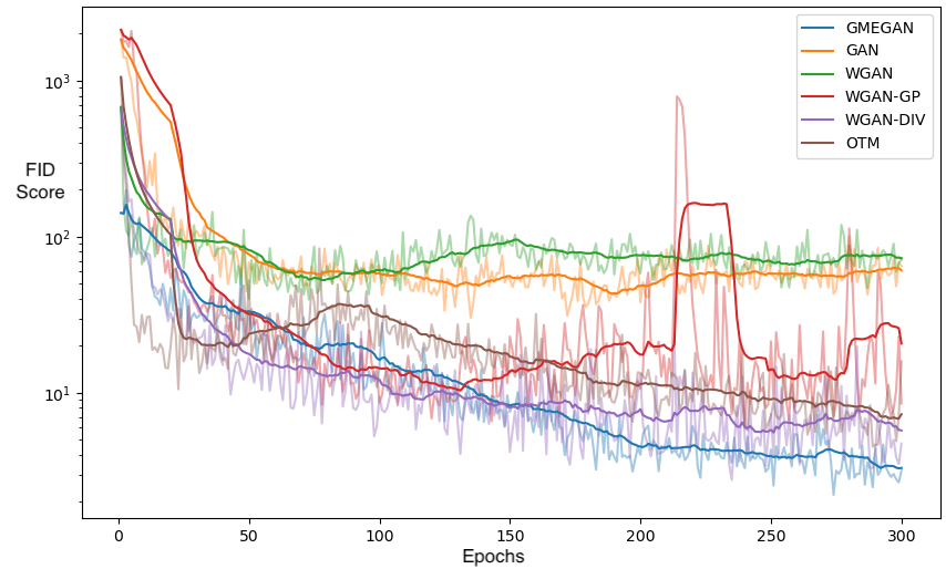
Figure 6. FID score plot with respect to epochs ranging from 0 to 300, trained with the CIFAR-10 dataset. The transparent lines represent the FID at each epoch, while the solid lines show a moving average by calculating the mean value over the previous 20 epochs.

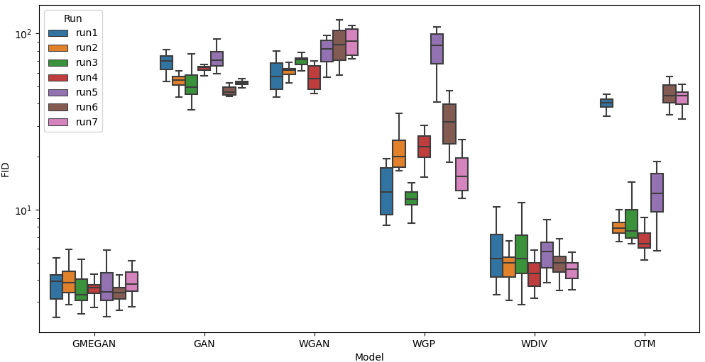
(a) FID scores from CIFAR-10

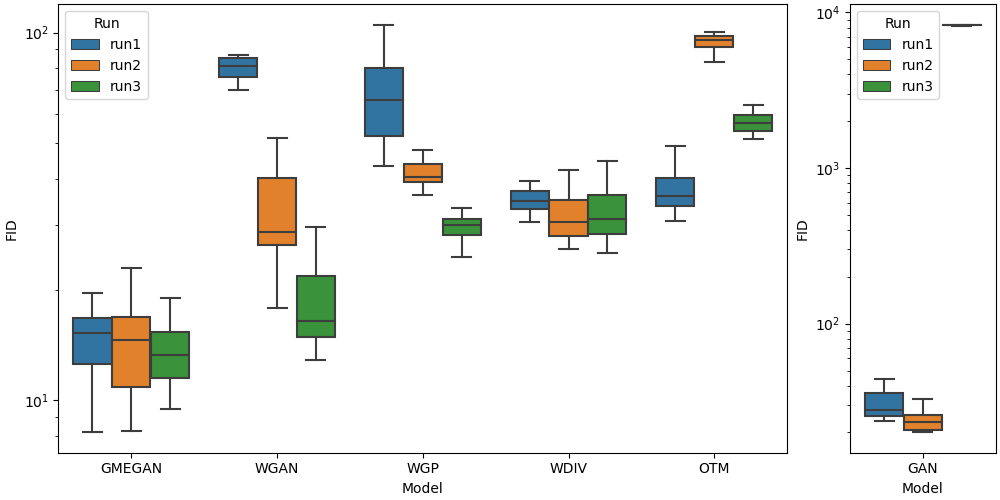
(b) FID scores from Celeb-A

Figure 7. Figure shows box plots that depict FID scores at epoch 300 for six distinct generative models. These plots are presented separately for the CIFAR-10 dataset (top) and the Celeb-A dataset (bottom).

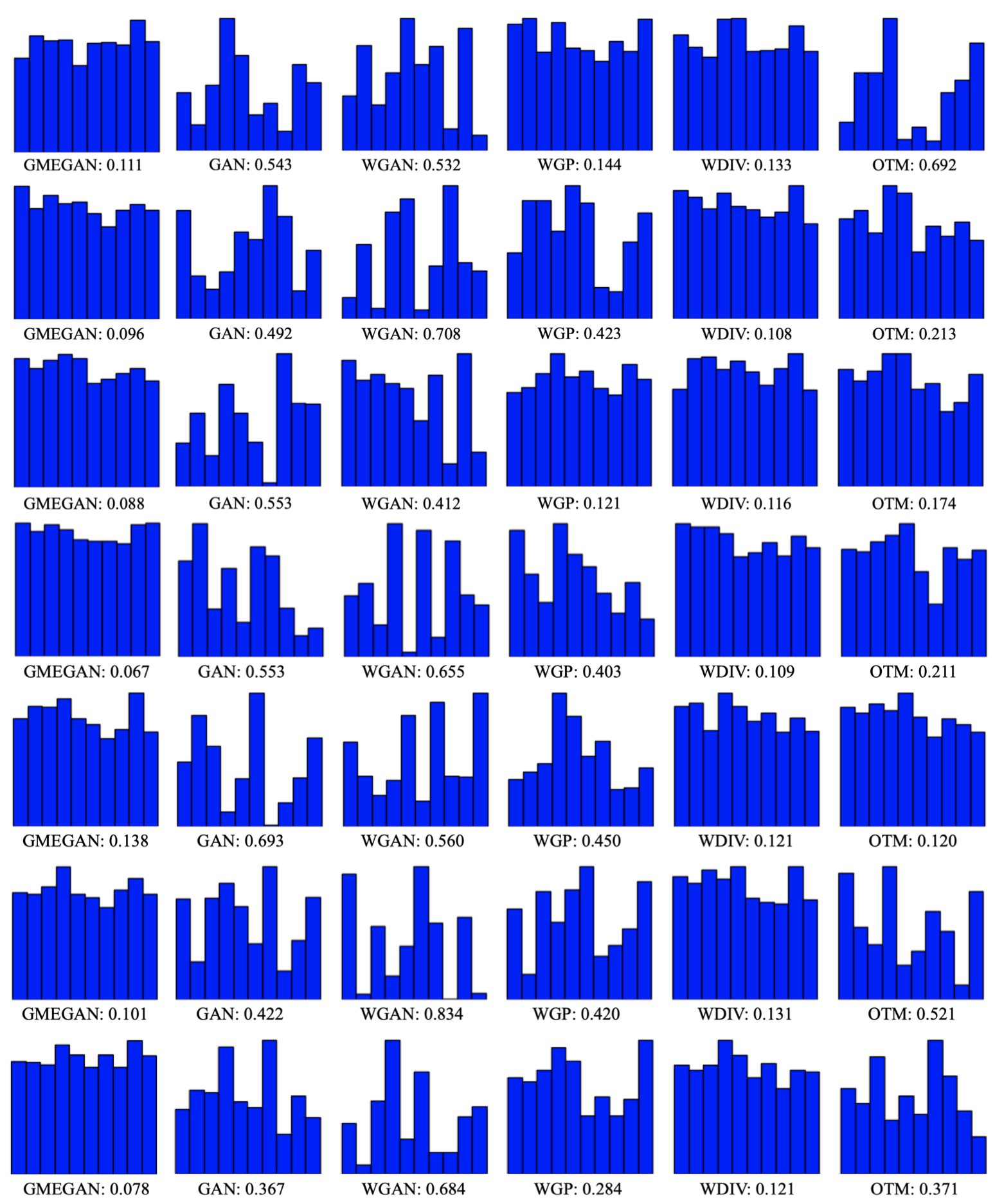
Figure 8. The histograms depict the generated samples in ten classes of images from each method, trained with the CIFAR-10 dataset. The relative standard deviations of the six methods are presented next to their respective names. A large relative standard deviation indicates the possibility of mode collapse. Each row displays the results at epoch 300 with different parameter initializations. The means and standard deviations of the relative standard deviations are presented in Table 6.

Table 6. The means and standard deviations of relative standard devi ations at epoch 300 from six methods. These means are calculated over seven different training sessions with different parameter initializations. The histograms of seven different training sessions are displayed in Figure 8.

GMEGAN	GAN	WGAN	WGP	WDIV	OTM
0.097 $\pm$ 0.02	0.517 $\pm$ 0.10	0.626 $\pm$ 0.13	0.320 $\pm$ 0.13	0.120 $\pm$ 0.01	0.328 $\pm$ 0.21

References

• AB [17] Martin Arjovsky and Leon Bottou. Towards principled methods for training generative adversarial networks. In International Conference on Learning Representations, 2017.
• ACB [17] Martin Arjovsky, Soumith Chintala, and Léon Bottou. Wasserstein generative adversarial networks. In International conference on machine learning, pages 214–223. PMLR, 2017.
• AGL+ [17] Sanjeev Arora, Rong Ge, Yingyu Liang, Tengyu Ma, and Yi Zhang. Generalization and equilibrium in generative adversarial nets (GANs). In Doina Precup and Yee Whye Teh, editors, Proceedings of the 34th International Conference on Machine Learning, volume 70 of Proceedings of Machine Learning Research, pages 224–232. PMLR, 06–11 Aug 2017.
• AMJ [18] David Alvarez-Melis and Tommi Jaakkola. Gromov-Wasserstein alignment of word embedding spaces. pages 1881–1890, October-November 2018.
• BAMKJ [19] Charlotte Bunne, David Alvarez-Melis, Andreas Krause, and Stefanie Jegelka. Learning generative models across incomparable spaces. In International conference on machine learning, pages 851–861. PMLR, 2019.
• Bre [87] Y. Brenier. Decomposition polaire et rearrangement monotone des champs de vecteurs. C. R. Acad. Sci. Paris Ser. I Math., 305:805–808, 1987.
• CRL+ [20] Lenaic Chizat, Pierre Roussillon, Flavien Léger, François-Xavier Vialard, and Gabriel Peyré. Faster wasserstein distance estimation with the sinkhorn divergence. Advances in Neural Information Processing Systems, 33:2257–2269, 2020.
• FMN [16] Charles Fefferman, Sanjoy Mitter, and Hariharan Narayanan. Testing the manifold hypothesis. Journal of the American Mathematical Society, 29(4):983–1049, 2016.
• GAA+ [17] Ishaan Gulrajani, Faruk Ahmed, Martin Arjovsky, Vincent Dumoulin, and Aaron C Courville. Improved training of Wasserstein GANs. Advances in neural information processing systems, 30, 2017.
• GAL [20] Amos Gropp, Matan Atzmon, and Yaron Lipman. Isometric autoencoders. arXiv preprint arXiv:2006.09289, 2020.
• GAW [18] Mevlana Gemici, Zeynep Akata, and Max Welling. Primal-dual Wasserstein GAN. arXiv preprint arXiv:1805.09575, 2018.
• GBC [16] Ian Goodfellow, Yoshua Bengio, and Aaron Courville. Deep Learning. MIT Press, 2016. http://www.deeplearningbook.org.
• GCKG [23] B. Ghojogh, M. Crowley, F. Karray, and A. Ghodsi. Elements of Dimensionality Reduction and Manifold Learning. Springer International Publishing, 2023.
• GHLY [21] Xin Guo, Johnny Hong, Tianyi Lin, and Nan Yang. Relaxed Wasserstein with applications to GANs. In ICASSP 2021-2021 IEEE International Conference on Acoustics, Speech and Signal Processing (ICASSP), pages 3325–3329. IEEE, 2021.
• GPAM+ [14] Ian Goodfellow, Jean Pouget-Abadie, Mehdi Mirza, Bing Xu, David Warde-Farley, Sherjil Ozair, Aaron Courville, and Yoshua Bengio. Generative adversarial nets. In Z. Ghahramani, M. Welling, C. Cortes, N. Lawrence, and K.Q. Weinberger, editors, Advances in Neural Information Processing Systems, volume 27. Curran Associates, Inc., 2014.
• HJA [20] Jonathan Ho, Ajay Jain, and Pieter Abbeel. Denoising diffusion probabilistic models. Advances in neural information processing systems, 33:6840–6851, 2020.
• HRU+ [17] Martin Heusel, Hubert Ramsauer, Thomas Unterthiner, Bernhard Nessler, and Sepp Hochreiter. GANs trained by a two time-scale update rule converge to a local nash equilibrium. Advances in neural information processing systems, 30, 2017.
• HZZ [22] Yan Huang, Tianyuan Zhang, and Huidong Zhu. Improving word alignment by adding Gromov-Wasserstein into attention neural network. In Journal of Physics: Conference Series, volume 2171, page 012043. IOP Publishing, 2022.
• KEA+ [21] Alexander Korotin, Vage Egiazarian, Arip Asadulaev, Alexander Safin, and Evgeny Burnaev. Wasserstein-2 generative networks. In International Conference on Learning Representations, 2021.
• KH+ [09] Alex Krizhevsky, Geoffrey Hinton, et al. Learning multiple layers of features from tiny images. 2009.
• KLG+ [21] Alexander Korotin, Lingxiao Li, Aude Genevay, Justin Solomon, Alexander Filippov, and Evgeny Burnaev. Do neural optimal transport solvers work? a continuous wasserstein-2 benchmark. In A. Beygelzimer, Y. Dauphin, P. Liang, and J. Wortman Vaughan, editors, Advances in Neural Information Processing Systems, 2021.
• KW [14] Diederik P Kingma and Max Welling. Auto-encoding variational bayes. In International Conference on Learning Representations, 2014.
• KZSN [20] Keizo Kato, Jing Zhou, Tomotake Sasaki, and Akira Nakagawa. Rate-distortion optimization guided autoencoder for isometric embedding in Euclidean latent space. In Hal Daumé III and Aarti Singh, editors, Proceedings of the 37th International Conference on Machine Learning, volume 119 of Proceedings of Machine Learning Research, pages 5166–5176. PMLR, 13–18 Jul 2020.
• LLWT [15] Ziwei Liu, Ping Luo, Xiaogang Wang, and Xiaoou Tang. Deep learning face attributes in the wild. In Proceedings of International Conference on Computer Vision (ICCV), December 2015.
• LQZ+ [22] Xinhang Li, Zhaopeng Qiu, Xiangyu Zhao, Zihao Wang, Yong Zhang, Chunxiao Xing, and Xian Wu. Gromov-Wasserstein guided representation learning for cross-domain recommendation. In Proceedings of the 31st ACM International Conference on Information & Knowledge Management, pages 1199–1208, 2022.
• LSC+ [19] Na Lei, Kehua Su, Li Cui, Shing-Tung Yau, and Xianfeng David Gu. A geometric view of optimal transportation and generative model. Computer Aided Geometric Design, 68:1–21, 2019.
• LYSP [22] Yonghyeon LEE, Sangwoong Yoon, MinJun Son, and Frank C. Park. Regularized autoencoders for isometric representation learning. In International Conference on Learning Representations, 2022.
• Mém [07] Facundo Mémoli. On the use of Gromov-Hausdorff distances for shape comparison. In PBG@Eurographics, 2007.
• Mém [11] Facundo Mémoli. Gromov–Wasserstein distances and the metric approach to object matching. Foundations of computational mathematics, 11:417–487, 2011.
• MHM [18] Leland McInnes, John Healy, and James Melville. UMAP: Uniform manifold approximation and projection for dimension reduction. arXiv preprint arXiv:1802.03426, 2018.
• MTOL [20] Ashok Makkuva, Amirhossein Taghvaei, Sewoong Oh, and Jason Lee. Optimal transport mapping via input convex neural networks. In International Conference on Machine Learning, pages 6672–6681. PMLR, 2020.
• NTOH [23] Nao Nakagawa, Ren Togo, Takahiro Ogawa, and Miki Haseyama. Gromov-Wasserstein autoencoders. In The Eleventh International Conference on Learning Representations, 2023.
• PCS [16] Gabriel Peyré, Marco Cuturi, and Justin Solomon. Gromov-Wasserstein averaging of kernel and distance matrices. In International conference on machine learning, pages 2664–2672. PMLR, 2016.
• PFL [18] Henning Petzka, Asja Fischer, and Denis Lukovnikov. On the regularization of Wasserstein GANs. In International Conference on Learning Representations, 2018.
• PZA+ [21] Phil Pope, Chen Zhu, Ahmed Abdelkader, Micah Goldblum, and Tom Goldstein. The intrinsic dimension of images and its impact on learning. In International Conference on Learning Representations, 2021.
• RKB [22] Litu Rout, Alexander Korotin, and Evgeny Burnaev. Generative modeling with optimal transport maps. In International Conference on Learning Representations, 2022.
• RM [15] Danilo Rezende and Shakir Mohamed. Variational inference with normalizing flows. In International conference on machine learning, pages 1530–1538. PMLR, 2015.
• San [15] Filippo Santambrogio. Optimal transport for applied mathematicians. Birkäuser, NY, 55(58-63):94, 2015.
• SSM [18] Shibani Santurkar, Ludwig Schmidt, and Aleksander Madry. A classification-based study of covariate shift in gan distributions. In International Conference on Machine Learning, pages 4480–4489. PMLR, 2018.
• TFC+ [19] Vayer Titouan, Rémi Flamary, Nicolas Courty, Romain Tavenard, and Laetitia Chapel. Sliced Gromov-Wasserstein. Advances in Neural Information Processing Systems, 32, 2019.
• TJ [19] Amirhossein Taghvaei and Amin Jalali. 2-Wasserstein approximation via restricted convex potentials with application to improved training for GANs. arXiv preprint arXiv:1902.07197, 2019.
• VdMH [08] Laurens Van der Maaten and Geoffrey Hinton. Visualizing data using t-SNE. Journal of machine learning research, 9(11), 2008.
• WHT+ [18] Jiqing Wu, Zhiwu Huang, Janine Thoma, Dinesh Acharya, and Luc Van Gool. Wasserstein divergence for GANs. In Proceedings of the European conference on computer vision (ECCV), pages 653–668, 2018.
• XLC [19] Hongteng Xu, Dixin Luo, and Lawrence Carin. Scalable Gromov-Wasserstein learning for graph partitioning and matching. Advances in neural information processing systems, 32, 2019.
• XLZD [19] Hongteng Xu, Dixin Luo, Hongyuan Zha, and Lawrence Carin Duke. Gromov-Wasserstein learning for graph matching and node embedding. In International conference on machine learning, pages 6932–6941. PMLR, 2019.