Multimodal and Force-Matched Imitation Learning with a See-Through Visuotactile Sensor
Abstract
Kinesthetic Teaching is a popular approach to collecting expert robotic demonstrations of contact-rich tasks for imitation learning (IL), but it typically only measures motion, ignoring the force placed on the environment by the robot. Furthermore, contact-rich tasks require accurate sensing of both reaching and touching, which can be difficult to provide with conventional sensing modalities. We address these challenges with a See-Through-your-Skin (STS) visuotactile sensor, using the sensor both (i) as a measurement tool to improve kinesthetic teaching, and (ii) as a policy input in contact-rich door manipulation tasks. An STS sensor can be switched between visual and tactile modes by leveraging a semi-transparent surface and controllable lighting, allowing for both pre-contact visual sensing and during-contact tactile sensing with a single sensor. First, we propose tactile force matching, a methodology that enables a robot to match forces read during kinesthetic teaching using tactile signals. Second, we develop a policy that controls STS mode switching, allowing a policy to learn the appropriate moment to switch an STS from its visual to its tactile mode. Finally, we study multiple observation configurations to compare and contrast the value of visual and tactile data from an STS with visual data from a wrist-mounted eye-in-hand camera. With over 3,000 test episodes from real-world manipulation experiments, we find that the inclusion of force matching raises average policy success rates by 62.5%, STS mode switching by 30.3%, and STS data as a policy input by 42.5%. Our results highlight the utility of see-through tactile sensing for IL, both for data collection to allow force matching, and for policy execution to allow accurate task feedback.
Index Terms:
Force and Tactile Sensing, Imitation Learning, Learning from Demonstration, Deep Learning in Grasping and ManipulationI Introduction
When humans interact with articulated objects such as doors or drawers, their hands and fingers commonly slip, roll, and generate significant frictional forces relative to the handle. To achieve the complex contact-rich behaviour described above, robotic manipulators would likely benefit from high-resolution tactile feedback as well as corresponding motor policies to quickly act in response to such feedback. Optical tactile sensors [1] combine a gel-based material with a small, inexpensive camera to yield rich tactile information [2] and are able to provide the requisite feedback for dexterous manipulation [3, 4]. A recently-introduced see-through-your-skin (STS) optical sensor variant combines visual sensing with tactile sensing by leveraging a transparent membrane and controllable lighting [5, 6]. This sensor enables perception of the full interaction, from approach, through initial contact, to grasping, pulling or pushing.
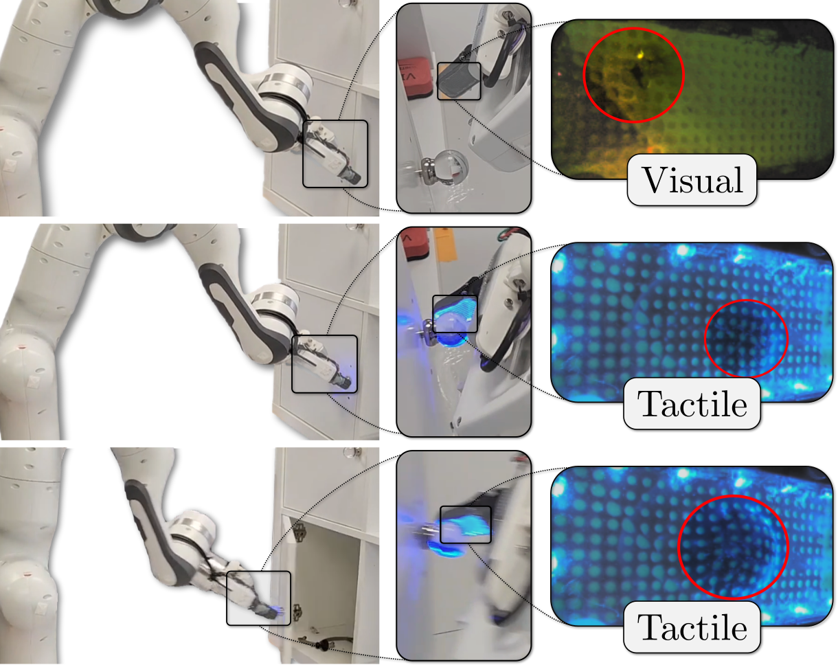
While prior work has investigated the use of hand-crafted controllers combined with STS sensing [6], simultaneously modelling dynamic effects like slip, roll, and frictional forces is challenging. An appealing alternative is to use imitation learning (IL), in which an expert provides a set of demonstrations of the task being completed, forming a dataset for training a policy. In this paper, we investigate how to leverage an STS sensor for IL on a real robotic platform for contact-rich manipulation tasks. We focus on the tasks of opening and closing cabinet doors with two challenging off-the-shelf components: a flat handle and a small, spherical glass knob. We complete these tasks with a 7-DOF robotic system that integrates a robotic finger outfitted with an visuotactile sensor (see Fig. 1), evaluating on four tasks in total. These tasks involve the complex contact behaviours previously described, including slip, roll, shear, and normal forces, but they also include an initial reaching component, motivating the use of an STS sensor over its standard, opaque counterpart.
Human-based expert demonstrations for IL can be collected in a variety of ways, though most methods fall generally into the kinesthetic teaching (in which a person directly moves and pushes the arm to complete a task) or teleoperation (in which a person remotely controls the robot through a secondary apparatus) categories [7]. While neither method is the definitive choice in all cases, kinesthetic teaching offers two specific major advantages over teleoperation: 1) a degree of haptic feedback is provided to the demonstrator, since they indirectly feel contact between the end-effector and the environment (similar to tactile feedback that humans feel during tool use), and 2) no extra devices beyond the arm itself are required. For the first point, teleoperation requires a proxy for true haptic feedback [8, 9], which can be costly and/or inaccurate. Additionally, prior work has found that kinesthetic teaching is preferred over teleoperation for its ease of use and speed of providing demonstrations [10, 11, 12].
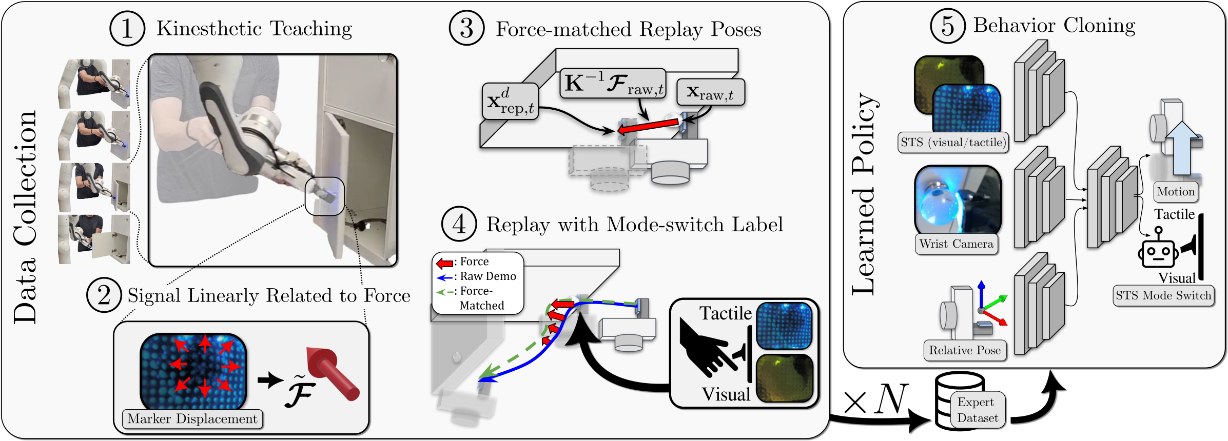
Unfortunately, kinesthetic teaching methods typically only measure a demonstrator’s motion, without considering the force placed on the environment by the robot. To match the demonstrator’s force profile, we require a means of measuring robot-to-environment forces, in addition to a mechanism for reproducing those forces. Our first contribution is a tactile force matching system that uses the readings from an STS sensor to modify the recorded poses from kinesthetic teaching. Our system generates a new trajectory of desired poses that, when used as input to a Cartesian impedance controller, recovers the recorded forces and poses to generate what we call a force-matched replay (see steps 2, 3 and 4 from Fig. 2). Compared with standard force control [13] and hybrid force-position control [14], our method does not actually require reasoning about true metric force or about specific axes of motion, making it simple to apply to an existing standard Cartesian impedance controller [15]. We measure a signal which is linearly related to force based on an estimated surface depth [16] using an STS sensor in tactile mode. This affords multiple advantages compared with typical approaches to force-torque sensing: (i) standard methods for measuring robot-to-environment force are corrupted by human-to-robot force as they move the robot (see Fig. 3 for clear examples), (ii) an STS is an order of magnitude less expensive than a similarly-mounted force-torque sensor, and (iii) the STS can be additionally used, in both visual and tactile modes, to provide dense information for learning policies.
To leverage both visual and tactile modes of an STS sensor, a method for deciding when to switch modes is required. Previous work [6] accomplished this using a combination of prior known objects and a separately trained object-specific detector. Our second contribution removes the assumption of known prior object and reduces this added complication with a novel method for switching between the visual and tactile modes of an STS sensor. We include mode switching as a policy output, allowing the demonstrator to set the sensor mode during the demonstration, which acts as a label for the expert dataset (see step 4 of Fig. 2). In addition to removing the need for prior knowledge and reducing the algorithmic burden of using an STS sensor, we find that this approach effectively learns to switch the sensor at the point of contact, and find that it significantly increases policy performance compared with single-mode sensing.
While tactile sensing and the use of visuotactile sensors has received increasing attention in recent years [1, 17, 18, 5, 6], the majority of manipulation systems still tend to exclude the use of it. At least one reason for this may be skepticism about whether the sensors actually provide a clear benefit for task completion that outweighs the cost of additional hardware and software. To help answer this question for door opening tasks, we complete an extensive experimental study to evaluate the benefits of including STS visual and tactile data (depending on the active mode) as input to a multimodal control policy. We compare the use of an STS sensor (both with and without mode switching) to the use of an eye-in-hand camera. While we are not the first to perform such a comparative observational study with tactile sensing [19] or a visuotactile sensor [20, 21], we are the first to do so with an STS sensor, and our tasks are notable for being standard, real-world tasks, as opposed to tasks that specifically require the use of tactile sensing, such as [21, 22, 23].
Our contributions can be summarized as:
-
1.
A novel force matching system for improving kinesthetic teaching demonstration data using a Cartesian impedance controller and sensing from a finger STS sensor.
-
2.
A novel approach to visual/tactile mode switching when using an STS sensor based on expert demonstrations and a learned policy.
-
3.
An empirical study of robotic door opening in which we test many variations of our observation space to consider the benefits of a multimodal visual/tactile sensor as a policy input in IL, specifically compared to using a wrist-mounted eye-in-hand camera and pose data.
In Section II, we detail the literature and fields that our work combines and builds upon, including sections on impedance control, visuotactile sensors, imitation learning, and visuotactile sensing combined with robotic manipulation. Section III details our imitation learning pipeline and how our novel force matching and mode switching additions fit into it, including a description of our method for data collection based on kinesthetic teaching, our force matching algorithm, our method for measuring a signal linearly related to force, and finally our visual/tactile mode labelling approach. In Section IV, we go through our experiments, first describing our environment and assumptions, followed by experiments and results on force matching, mode switching, observation space variations, and expert data scaling. Finally, in Section V we describe the limitations of our work, while in Section VI we provide concluding remarks.
II Related Work
Our work can be situated within the literature at the intersection of imitation learning, tactile sensing, and impedance control. We start by discussing the use of force for control in manipulation, and how this methodology contrasts with our approach. This leads into a survey of visuotactile sensing, see-through sensors, and the use of these sensors for measuring signals such as force. Next, we provide a short background on imitation learning (IL) and its application to robotic manipulation. We describe how IL can be improved by combining work from both of the aforementioned topics. Finally, we discuss other work that combines visuotactile sensing with manipulation, noting specific differences with our own research.
II-A Impedance and Force Control
Impedance control is an approach to robotic control in which force and position are related by a theoretical mass-spring-damper system [15], and desired poses are chosen along with tuned stiffness and damping parameters to allow compliance with the environment. Impedance control can be easier to employ in robotic manipulation than closed-loop force control [13] because the contact dynamics between the robot and the environment are often difficult to model. Unfortunately, being an indirect force control method [24], applying desired forces in this scheme is not possible, and hybrid position/force control must be used instead [14]. In our work, we use kinesthetic teaching to generate initial position-only trajectories while measuring a signal linearly related to force. This signal, which we measure with a visuotactile sensor, is used to modify demonstrator trajectories so that, when input into the original impedance controller, the new trajectories reproduce both the original path and the applied forces.
II-B Visuotactile Sensors
The development of gel-based optical tactile sensors has led to a wide range of research on dense tactile feedback [2, 3, 4]. Adding a semi-transparent polymer on top of these sensors allows for both visual and tactile sensing [17], and is further improved through the addition of controllable lighting [5]. These sensors can be used to measure normal and shear forces through the tracking of printed dots embedded in the sensor membrane [25, 4, 26] and with finite element analysis [25, 4]. In our work, we do not require true ‘metric’ force, so the complication of the above methods, which require a force-torque sensor for calibration, is unnecessary. We instead estimate a signal linearly related to force based on the average estimated surface depth, using an algorithm from concurrently submitted work which estimates the depth through dot displacement [16].
II-C Imitation Learning
Imitation learning (IL) is an approach for training a control policy given a set of expert demonstrations of the desired behaviour. IL can generally be separated into methods based on behaviour cloning [27], in which supervised learning is carried out on the expert demonstration set, or inverse reinforcement learning [28], where the expert’s reward function is inferred from the demonstration set. Both behaviour cloning [8, 29, 30] and inverse reinforcement learning [31, 32, 33] have been used successfully for many robotic manipulation tasks. Recent applications tend to avoid the use of kinesthetic teaching [7] in favour of teleoperation, despite the ability of the former to provide a degree of haptic feedback to the demonstrator. Teleoperation requires a proxy system to provide haptic feedback [8, 9] that may be inaccurate or expensive.
Although we do not compare teleoperation with kinesthetic teaching in our research, previous work has shown kinesthetic teaching to be preferred for many tasks for its ease of use and speed of demonstration [10, 11, 12]. Previous work that combines kinesthetic teaching with force profile reproduction requires one demonstration for positions and a separate demonstration for forces [34], which can be inconvenient and challenging to provide. In our work, the demonstrator provides a single demonstration including both desired poses and forces through kinesthetic teaching, which is then combined with our novel force matching algorithm to generate our expert dataset.
II-D Visuotactile Sensing and Robotic Manipulation
Learning-based manipulation tasks have benefited from the use of contact sensing [35, 19], as well as optical tactile sensors for both reinforcement learning [20] and imitation learning [36, 21]. Our learning architecture is similar to [21], in which tactile, visual, and auditory data is combined in a single neural network and trained with behaviour cloning. In [21], demonstrations are collected primarily with scripts for very specific tasks with a bespoke system. In contrast to [21], we use kinesthetic teaching without any task-based assumptions or scripted policies, which can generalize to many tasks, and demonstrate how the tactile sensor can be used to directly improve the demonstrations themselves.
Our work is closely related to [6], which uses a multimodal tactile sensor to complete a bead-maze task with a robotic manipulator. In contrast, our tasks require a combination of normal force, shear force, grip, slip, and roll for which it would be difficult to handcraft a policy, so we learn closed-loop motion actions end-to-end through imitation learning instead. Additionally, our policy learns mode-switching actions directly, whereas [6] uses a separate model and algorithm with specific domain knowledge.
III Methodology
In this section, we introduce each component of our system. We formulate our IL problem as a Markov decision process (MDP) in Section III-A, described in Section III-A. In Section III-B and Section III-C, we develop our Cartesian impedance control law and explain its relationship to kinesthetic teaching. We then present our methods for (i) match expert demonstrator forces (Section III-D), (ii) using a signal linearly related to force instead of true force (Section III-E), (iii) measuring these signals (Section III-F), and (iv) collecting sensor mode labels (Section III-G). Finally, we provide our training objective in Section III-H.
III-A Problem Formulation
A Markov decision process (MDP) is a tuple , where the sets and are respectively the state and action space, is a reward function, is the state-transition environment dynamics distribution and is the initial state distribution. Actions are sampled from a stochastic policy . The policy interacts with the environment to yield the experience for , where , and is the finite horizon length.
We aim to learn a policy that maximizes the expected return , where is the trajectory starting with , and is the return of trajectory .
In this work, we focus on imitation learning (IL), where is unknown and instead we are given a finite set of task-specific expert demonstration pairs , .
III-B Impedance Control
We start by describing the impedance control law, before explaining how it can be applied to kinesthetic teaching and then later to our approach to force matching. The Cartesian impedance control equation that relates external forces to position, velocity, and acceleration is
| (1) |
where represents the generalized external force, is the difference between desired and current pose, and are the manually tuned stiffness and damping (diagonal) matrices, is the fixed inertia matrix that is determined based on known end-effector parameters, and is a term encompassing generalized force of Coriolis, centrifugal, and gravitation based on current joint positions and velocities, and . In our case, is a six-dimensional external wrench since we control the robot in six degrees of freedom (three translational, three rotational). We treat the rotational components of as and , where refers to the world frame, to the current robot frame, to the desired frame, and is the passive rotation from frame to frame . The rotation error is , which we convert to an axis-angle representation.
On our robot, we control joint torques111Note that our symbol for joint torques does not refer to a vector form of a trajectory . We choose these symbols in our best effort to be consistent with existing literature on both force control and imitation learning. instead of force directly, so we can use the from Eq. 1 and the current manipulator Jacobian to obtain
| (2) |
To simplify further analysis, we will consider the case where each desired pose is in static equilibrium and gravity compensation is handled separately (by and from Eq. 1), so the general impedance control law Eq. 1 simplifies to the standard spring relationship as
| (3) |
where is the current timestep. The relationship between the static control law in Eq. 3 and our actual controlled joint torques from Eq. 2 is
| (4) |
where indicates that the joint torques are desired control setpoints. Substituting Eq. 3 into Eq. 4 yields
| (5) |
illustrating that measuring end-effector contact forces is not required by the indirect control scheme employed by a standard impedance controller [24]. We note, however, that this formulation leaves out damping, Coriolis, and nullspace terms, which are calculated by measuring gravitational forces. The impedance controller takes exclusively desired positions as input and produces the required joint torques as output; the resultant, applied force is simply a consequence of Eq. 1.
III-C Data Collection with Kinesthetic Teaching
In this section, we provide further detail on our method for collecting raw demonstrations via kinesthetic teaching, how it connects to our impedance controller, and why this method motivates tactile force matching. We collect one expert dataset for each task separately using kinesthetic teaching, in which the expert physically pushes the robot to collect demonstrations [7] (see Fig. 2 as well as our supplementary video for examples of what this looks like on our real system). A popular and relatively simple means of implementing kinesthetic teaching is through torque-based Cartesian impedance control. To allow for demonstrations via kinesthetic teaching, we set from Eq. 3 very close to zero, ensuring the robot has full compliance with the environment. We then record expert end-effector poses at a fixed rate as the robot is moved by the human, and use these poses, or, equivalently, the changes between poses, as expert actions [7] (for further discussion on the choice between absolute poses or changes between poses for our action space, see Section IV-A). While this recording process is one part of our approach, it suffers from at least two limitations:
-
1.
Recording the end-effector poses as the robot is moved means that the corresponding states and actions may not accurately reflect and .
-
2.
If the expert generates motion in which a wrench is applied between the robot and the environment with no corresponding change in , this approach will fail to reproduce that wrench.
An example of Item 1 above for would be the presence of the human demonstrator, or even a shadow from the human demonstrator, in the frame of a camera being used to generate . For , it is impossible to guarantee that the controller can perfectly reproduce the motion generated under full compliance while the human is pushing the arm.
Item 1 can be resolved with replays, in which the demonstrator collects a single demonstration trajectory , resets the environment to the same , and then uses a sufficiently accurate controller to reproduce each [37]. For trajectories in free space or where minimal force is exerted on the environment, this can be enough to learn effective policies [38, 37, 39]. Because we are interested specifically in tasks where significant force application is required, resolving Item 2 requires additional sensory input, as we discuss in the next section.
III-D Tactile Force Matching
In this section, we explain our method for generating force-matched replays of our raw kinesthetic teaching trajectories under the assumption that that the true external wrench at the point of contact on the end-effector can be measured. In Section III-E, we relax this assumption and consider using a signal linearly related to the wrench instead.
Consider a raw demonstrator trajectory of recorded end-effector poses and wrenches as a set of poses and wrenches that we would like our controller to achieve. We start by inverting the spring relationship in Eq. 3 to show how we can instead solve for desired (replay) positions that would generate particular forces given a fixed stiffness matrix as
| (6) |
as illustrated in the replay pose generation step of Fig. 2. Taking the modified desired replay poses from Eq. 6 and substituting them into Eq. 5 as our new desired poses, we have
| (7) |
Eq. 7 shows that, in actuality, we have modified the controller with an open-loop term for directly reproducing , assuming static conditions, while maintaining the same original stiffness/impedance control term for reproducing . In cases where , our approach acts as a standard impedance controller.
We consider the stiffness to be a fixed hyperparameter (typically a diagonal matrix with one value for all translational components, and another for all rotational ones), selected to optimally trade off control accuracy and environment compliance. Using Eq. 6, we can generate a trajectory of replay pose setpoints , a new set of poses that, under static conditions, would reproduce the both the positions and the forces from the raw kinesthetic teaching trajectory. In reality, we desire smooth, continuous motion and the simplification assuming static conditions does not account for dynamic effects. Experimentally, we find that when we input as a set of desired poses for our Cartesian impedance controller, we achieve replayed pose trajectories and force trajectories that sufficiently match and .
III-E Visuotactile Sensing as a Signal Linearly Related to Force
In this section, we relax our previous assumption and show how we can generate force-matched replay trajectories without access to true external wrench measurements, instead using a signal linearly related to force. We also discuss options for acquiring this signal, motivating our use of the STS sensor. Finally, we detail our procedure for finding the relationship between this signal and robotic motion with our previously described impedance controller.
To generate replay trajectories with Eq. 6, we require a means of sensing environment-robot forces . In common approaches for sensing end-effector forces on robotic arms, such as wrist-mounted force-torque sensors or joint-torque sensors with dynamics modelling, is corrupted by the demonstrator’s own force against the robot. To avoid this corruption, a sensor must be mounted at a point on the end-effector where human-applied forces are ignored during demonstrations, such as on the finger of a gripper. While finger-mounted force-torque sensors exist, we use a see-through visuotactile sensor because of its low cost, its ability to be reused as a source of data for control policies, and because we do not require true, metric force .
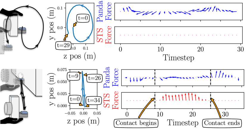
In Fig. 3, we show the results of a set of simple demonstrations to illustrate how the forces recorded from on-board joint torque sensors cannot isolate environment contact forces from human contact forces, and how our linearly related force signal from the STS resolves this problem. The trajectories shown correspond to (i) pushing an arm in a circle without environmental contact, and (ii) pushing an arm towards, against, and away from a fixed knob. The STS sensor correctly shows no readings in the circular trajectory, where there is no contact, and shows increasing and then decreasing force during contact in the trajectory where it is pushed against the knob. Conversely, the Panda force readings are primarily in response to the human pushing force against the robot, making it impossible to segment out the forces between the end-effector and the environment.
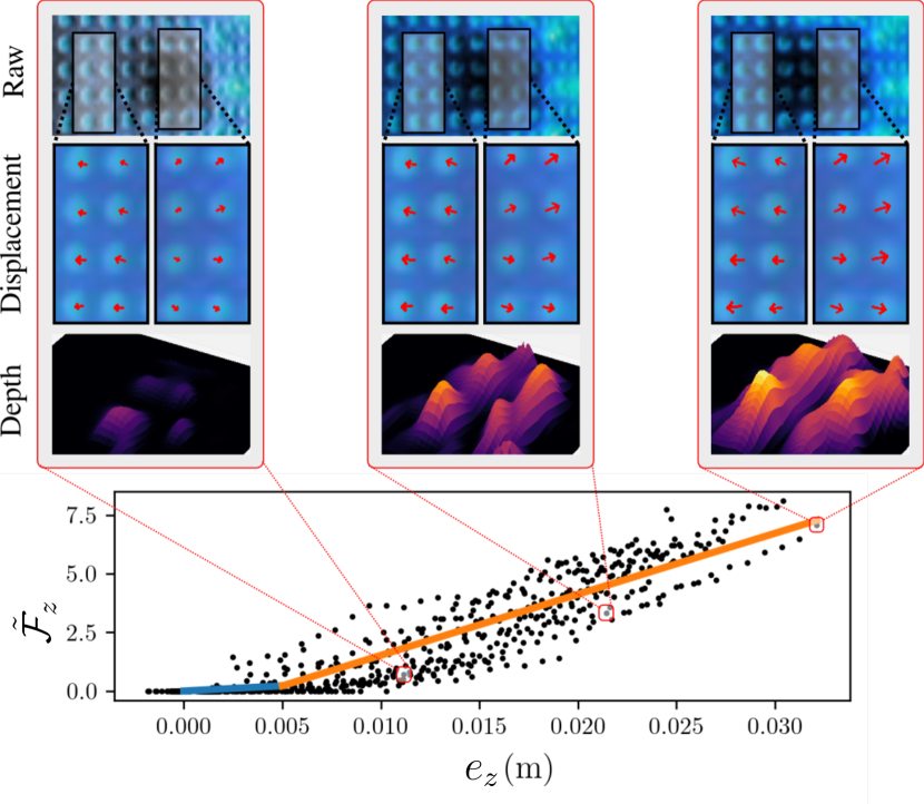
Here we will elaborate on how we can avoid the use of hard-to-acquire or potentially corruptible metric force, and outline how we can modify Eq. 6 to generate using , which we define as a signal linearly related to force. We describe how we acquire this signal in Section III-F. Since is not true force, it cannot be used directly in Eq. 6 or in Eq. 7. However, assuming is linearly related to , we have
| (8) |
which, after solving for and (where and are a matrix and vector describing the linear relationship between x and y), we could then rearrange to directly sub into Eq. 6 and Eq. 7. However, solving for and would still require a means of measuring true metric force at the point of contact, which we do not assume to have.
Instead, we can directly find a relationship between pose error and based on the spring relationship in Eq. 3 through a short data collection procedure and solve a least squares problem, similar to many other calibration procedures. For brevity, for the remainder of this section, we drop the superscript when referring to . We elect to use a piecewise linear model for the relationship between and (in all dimensions), as the relationship between surface depth and normal force for optical tactile sensors has previously been shown to be linear [25], though a more accurate model may exist. The simplified relationship is
| (9) |
where we have removed the piecewise component for brevity.
To find and , we use a scripted policy to incrementally push the sensor against the static environment numerous times, providing small initial perturbations to each trajectory to increase robustness. To also generate shear, we include lateral movement of the sensor relative to the knob, and to generate torque, we include rotational movement. Throughout these trajectories, we measure and record and . We subsequently use least squares to solve for and . The measured calibration values and the piecewise linear relationship between the -axis error and normal forces are shown in Fig. 4. For further description of specific design choices related to this procedure in practice, see Section IV-A.
An advantage of this approach is that it is valid for any type of sensor that is capable of reading a signal linearly related to force (e.g. visuotactile, pressure, or strain-gauge sensors). During kinesthetic teaching, we keep our sensor in tactile mode so that we can always read . We only allow mode switching during replays, when reading is no longer required. Another advantage of this approach is that any repeatable control errors (where true torques do not match desired torques specified in Eq. 4) or mild physical deformation of the sensor housing are accommodated, whereas simply using a force-torque sensor with Eq. 6 would not handle these issues.
We identify at least two sources of error in this procedure: (i) measurement errors, where the same value will result in different values for (and cannot be accounted for by noise alone), and (ii) model errors, where a linear model may not adequately define the relationship between these two quantities. The variability in Fig. 4 shows that these sources of error have a non-negligible effect, but our experimental results show that this approach still realizes improved performance and matching of demonstrator trajectories.
III-F Force Measurement
In this section, we provide further detail on how we measure a signal linearly related to force with a visuotactile sensor. We measure these signals in a variety of ways depending on the specific degree of freedom, although all are based on marker tracking. Note that our see-through-your-skin (STS) sensors contain painted-on markers or dots (see Fig. 4 for examples of these markers and their tracked displacements), as is common in many recent iterations of visuotactile sensors [6, 5, 2]. We track the locations of these markers in the RGB camera using OpenCV’s adaptive threshold [40] as well as common filtering strategies, including low-pass filtering and a scheme for rejecting outlier marker displacements based on nearest neighbour distributions.
For normal force, we use a method for estimating membrane depth, where depth is inferred from marker movement on the surface of the membrane, as shown in Fig. 4 [16]. Using a perspective camera model, [16] models a relationship between the separation of markers locally, and the amount of displacement towards the camera, allowing dense depth to be recovered using properties of a local distance transform. We use the average of each of these marker depths for the normal force . Fig. 4 shows examples of both dot displacement and corresponding estimated depth at all points as the knob is pushed against the sensor, as well as our corresponding estimates for for a set of individual points. The bottom of Fig. 4 also shows that the relationship between and is reasonably piecewise linear (and linear for a large portion of the change in ), indicating that this relationship is a suitable replacement for the spring relationship between true, metric force and displacement described by Eq. 3.
For signals linearly related to shear forces, we use the average of the tracked dot movement in both the horizontal and vertical directions parallel to the sensor plane, For signals linearly related to torque, we use the average of the tracked dot movement that is perpendicular to an estimate of a center point of maximal normal force. We do not measure torque about the axes parallel to the surface because it is unclear how one would differentiate between measurements of this torque and measurements of shear. Empirically, we find that these extra degrees of freedom are not necessary for generating a successful .
To use these measurements of force and apply them to the robot frame, a transform between the measurement frame of the sensor and the robot tool frame is necessary. While it would be possible to calibrate these two frames using standard eye-in-hand manipulator calibration [41] or a form of touch-based eye-in-hand calibration [42], we find that assuming a fixed transformation is suitable for our setup. In our case, this is because the STS is mounted to the gripper such that its principal axes require exclusively 90-degree rotations to recover the default end-effector control frame. Further reducing the need for such calibration is the fact that the center of the sensor surface corresponds to our assumed tool frame, so our sensor-to-tool-frame transform’s translational component is zero.
III-G STS Sensor Mode Labelling


The STS sensor used in this work is a more compact, robotic-finger-sized version of the model described in [6]. Compared to standard visuotactile sensors [25, 4], it has a semi-transparent membrane and a ring of surrounding, controllable LED lights, as shown in Fig. 5.222See [6] for further details on the the construction of the sensor. As previously noted, it can operate in two modes:
-
•
Visual mode, where the internal STS LEDs are turned fully off, allowing for the camera to see through the membrane to approach and to identify aspects of the scene before contact has been made.
-
•
Tactile mode, where the internal STS LEDs are turned on to a pre-calibrated level, enabling the camera and dotted membrane to operate as a standard visuotactile sensor, providing detailed contact feedback.
An STS sensor requires a method to control switching between visual and tactile modes. In [6], this switch was accomplished through the use of known object appearance and size combined with a separately trained object detection model to determine approximate object distance from the sensor membrane. To remove the assumption of prior known object models as well as reduce algorithmic complication, we instead treat the mode switch as an output from our control policy, and allow the human demonstrator to switch the mode of the sensor during the demonstration. The rest of this section describes our method for collecting these labels.
After each kinesthetic teaching trajectory, the expert manually triggers the STS mode switch from visual to tactile during the replay phase. As the controller autonomously generates , the demonstrator observes and presses a button to change the sensor mode. This mode change is also used as an action label for training policy outputs. This approach ensures that the visuotactile images that are added to the expert dataset contain both visual and tactile data, since the initial demonstration of had the sensor mode exclusively set to to tactile mode to ensure the signal linearly related to force was accurately read throughout the motion. Furthermore, since our force matching system already requires replays of demonstrations, this requires minimal extra effort from the demonstrator.
A particular advantage of this technique, especially when compared with an external algorithm such as [6] that is tuned specifically to change modes at the point of contact, is that the demonstrator can choose on a task-by-task basis whether the sensor mode switch should occur before contact, at the point of contact, or after contact. Tasks that require tracking right up until the point of contact may benefit from having the mode switch occur post-contact, while tasks which require a delicate and less forceful touch/grasp may benefit from the opposite. In theory, a demonstrator could actually provide numerous switches throughout a trajectory for tasks that might require it, which is also not possible in [6], but we did not explore tasks of this nature.
III-H Policy Training
Our policies are trained with a standard mean-squared-error behaviour cloning loss,
| (11) |
where and . can include any or all of raw STS images, wrist camera images, and robot pose information, while includes motion control and sensor mode commands (see Section IV-A for more details).
IV Experiments
Through our experiments, we try to answer the following questions:
-
1.
What is the benefit of force matching for policies learned with imitation learning (IL) and kinesthetic teaching?
-
2.
What is the benefit of our policy mode switching output for policies learned with IL?
-
3.
Is a see-through visuotactile (STS) sensor a required policy input for our door manipulation tasks, or is a wrist-mounted eye-in-hand camera sufficient?
-
4.
Can an STS sensor alone (i.e., without any other external sensor) provide sufficient visual and tactile information to solve our door manipulation tasks, and if so, what is the benefit of including mode switching?
In Section IV-A, we describe our experimental environment and task parameters, including how we set up our robot. Next, we report performance results on our system as a whole in Section IV-C, the benefits of using force matching in Section IV-D, and the benefits of our policy mode-switching output in Section IV-E. We follow with the results of our observational space study in Section IV-F, followed by the results of training and testing policies with exclusively STS data in Section IV-G. Finally, as is common and useful in imitation learning in general, we present results on expert data scaling in Section IV-H.
IV-A Environment and Task Parameters
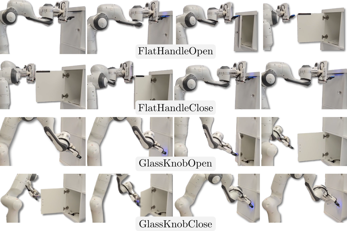
We study the robotic task of cabinet door opening and closing, using one door with a flat metal handle and one with a spherical glass knob (see Fig. 6 for close-ups of both), giving us four total experimental tasks, hereafter referred to as FlatHandleOpen, FlatHandleClose, GlassKnobOpen, and GlassKnobClose. All tasks include an initial reaching/approach component (see Fig. 6, Fig. 7, and Fig. 8), where the initial pose of the robot relative to the the knob or handle is randomized. Choosing these tasks allows us to collect data and test policies more quickly, since successful execution of each task resets the environment for its counterpart [43]. These tasks represent a wider class of manipulation tasks where traditional sense-plan-act system architectures are likely to fail, because these tasks require the handling of complicated contact dynamics including slip, roll, friction, and force, motivating the use of an end-to-end learning approach with tactile sensing (see Fig. 8 for visual examples of the continuous slipping between the finger and the knobs/handles throughout demonstrations).
Door opening tasks are considered successful if the door fully opens within a given time limit. Door closing tasks are considered successful if the door closes without “slamming”: if the knob or handle fully slips off of the finger before the door is closed, the spring hinges cause it to loudly slam shut. In either case, failure occurs because the finger loses contact with the handle or knob before a motion is complete, which can occur easily since the tasks require some degree of roll and slip to complete.
Our robotic platform is a Franka Emika Panda, and we use the default controller that comes with Polymetis [44] as our Cartesian impedance controller. For all tasks, at the beginning of each episode, the initial pose of the end-effector frame is randomized to be within a 3 cm 3 cm 3 cm cube in free space, with the rotation about the global -axis (upwards facing) randomized between and radians. Our task environments can include wrist camera 212 120 pixel RGB images, raw 212 120 STS images (in either visual or tactile mode), and the current and previous relative end-effector poses (position, quaternion). In this work, relative poses means that in each episode, the initial pose is set to , even though the global pose is randomized for every episode, as previously described. These choices were meant to simulate the scenario in which an approximate reach is performed with an existing policy and global pose information between episodes is inconsistent (e.g., in the case of a mobile manipulator in a larger environment), similar to prior work using an actual mobile manipulation platform [8]. Including pose information as an input into a learned policy is common [45, 8], but recent work has questioned whether it definitively provides benefit [29]. In Section IV-F1, we investigate the value of pose information for our tasks and sensor suite.
Our sensor is based on the one developed in [6], but in a smaller form factor. For more details on sensor design and manufacturing, see [6, 5]. The finger housing is 3D printed and mounted on the Franka Emika Panda gripper. Due to the fragility of the top layer of the original sensor, especially when subject to large shear forces as required by our tasks, we use the sensor with this top layer, as well as the semi-reflective paint, fully removed. This choice would potentially pose a problem for model-based approaches to using an STS, but in our case, learned policies are able to handle tactile data where the sensor is not fully opaque. The LED values and camera parameters for the sensor are set using a simple calibration tool, in which our marker detection algorithm runs alongside a set of tools for modifying the camera parameters (such as exposure time and white balance) and LED intensity levels.
As detailed in Section III-F, a short calibration procedure allows us to solve for the parameters in Eq. 10. This calibration procedure takes about seven minutes in practice, and is fully autonomous. We use our glass knob as the calibration object, and move the desired pose of the end-effector 3.5 cm towards the glass knob while moving at 1mm increments, with each trajectory starting between 1 mm and 3 mm away from touching it to start. We also generate shear by moving 1cm laterally, and torque by moving 1rad rotationally, after already having made initial contact with the knob. See our supplementary video for a full example of our calibration procedure.
IV-B Imitation Learning and Training Parameters
Demonstrations are collected by allowing a user to press a button that switches the stiffness and damping on the controller to nearly zero. Data is then collected at a predefined rate (10 Hz in our experiments) once the robot has exceeded a minimum initial movement threshold (0.5 mm in our experiments). After the kinesthetic demonstration is completed, the environment is reset to the same initial (global) pose, and the demonstration is replayed. During the replay, we optionally use altered desired poses to allow force matching (see Sections III-D and III-F), and also optionally allow the user to switch the mode of the sensor (simultaneously providing a mode-switch label, see Section III-G).
For all imitation learning experiments with expert datasets, we collected 20 “raw” kinesthetic teaching demonstrations with a human expert per task (80 total). With these raw demonstrations, we completed replay trajectories in a variety of configurations (further described in sections Section IV-D, Section IV-E, and Section IV-H), depending on which algorithm we were testing. A benefit of this approach is that we were able to not only minimize the required human labour of completing demonstrations, but we were also able to more directly compare the benefits of including force matching and mode switching since the raw human trajectories were identical for each configuration. For every trained configuration, we train policies with three different random seeds, and complete 10 test episodes (with different random initial environment configurations from those used during training) per seed.
We trained our policies in PyTorch with the Adam optimizer and a learning rate of 0.0003, halving the learning rate halfway through training. We use a ResNet-18 [46] architecture pretrained on ImageNet and ending with spatial soft-argmax [45] for image data, and a small fully connected network for relative pose data. Features from each modality are concatenated and passed through another small fully connected network before outputting our seven-dimensional action: relative position change, orientation change as a rotation vector, and STS mode. All layers use ReLU non-linearities. We train each policy for 20k gradient steps, using weight decay of 0.1 to avoid overfitting, as this has been shown to dramatically improve behaviour cloning results in recent work compared to early stopping [29, 31].
IV-C System Performance
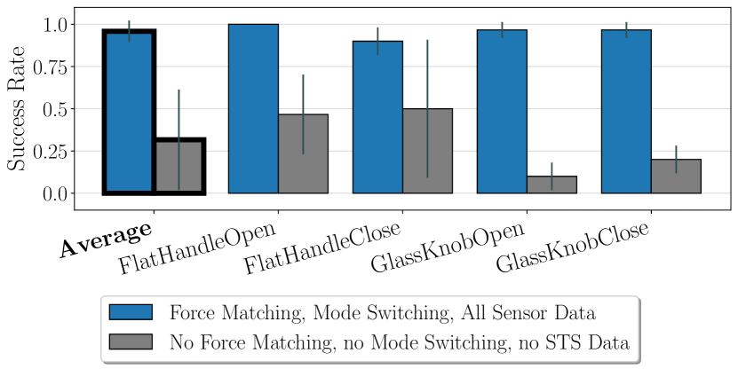
We evaluate the benefits of collectively including force matching, mode switching as a policy output, and STS data as a policy input by training policies including all three of these additions, as well as policies with none of them, and comparing their success rates. As previously stated in Section IV-B, we trained three seeds per task with 10 test episodes per seed, meaning we have 30 episodes for each task and configuration, and 120 total test episodes per configuration. This comparison is visualized for each individual task, and with an overall average across all tasks, in Fig. 9. Including these three additions results in a 64.2% average absolute across-task performance increase over the baseline where none are included, demonstrating a clear benefit. There is a task-related correlation, where the average improvement for the FlatHandle tasks is 46.7%, while the average improvement for GlassKnob tasks is 81.7%. These results alone, however, do not indicate how much each individual component contributes to policy performance. The remaining experimental sections ablate each of these additions individually to better understand each component’s contribution.
IV-D Force Matching Performance
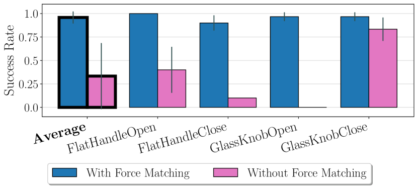
To evaluate the benefit of our force matching algorithm, we completed replays of our raw expert datasets both with and without force matching and compared their performance. To isolate the benefits of force matching, and reduce the effect of including/excluding policy mode switching, we included policy mode switching in both configurations, and we also included all three sensing modalities (wrist-mounted eye-in-hand RGB images, STS images, and relative positions) in both. For experiments where we vary the included sensing modalities, see Section IV-F. The results of our force matching policy performance tests are shown in Fig. 11.
The average absolute across-task performance increase of using force matching is 62.5%. While the overall trend is that force matching always provides a benefit, the performance gain is higher for some tasks than others. A particularly notable case is the discrepancy between gains for the two GlassKnob tasks: the GlassKnobOpen policy never succeeds without force matching, while the GlassKnobClose policy only has a slight benefit from force matching. This can partially be explained by the pose angle for much of the demonstration. For the GlassKnobOpen task, after contact is made with the knob, the door is almost exclusively pulled with a shear force. In this case, poor initial contact caused by too little force inevitably results in failure (see third column, third row of Fig. 10). In contrast, in the GlassKnobClose task, the angle of the robot finger relative to the knob ensures that normal force still occurs throughout much of the trajectory. While there is a slight delay in the re-generation of demonstrated forces for replays of this task (see fourth column, third row of Fig. 10), much of the trajectory ends up matching the demonstrated forces.
IV-D1 Force Matching Trajectory Comparison
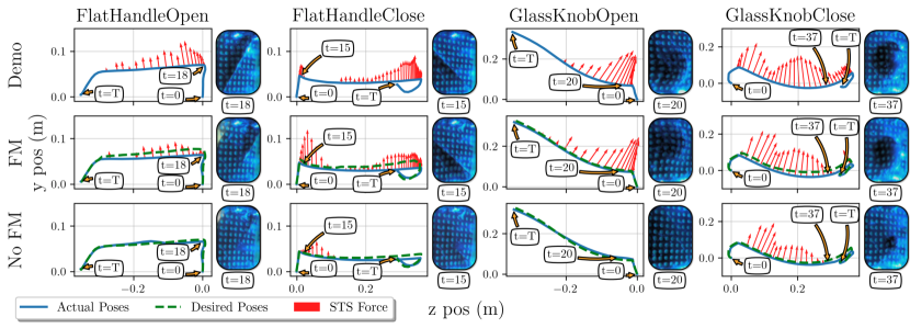
While our policy learning experiments in Section IV-D implicitly illustrate the value of force matching through improved performance, Fig. 10 shows specific examples of how trajectories change with and without force matching:
-
•
Top: a raw demonstration trajectory (blue) as well as demonstration forces (red).
-
•
Middle: a new set of desired poses that incorporate force matching (green), the new set of replayed poses given (blue), and the actual forces with the modified trajectory (red).
-
•
Bottom: a set of desired and actual poses, along with resulting forces, that use directly (i.e., without force matching), while ignoring , to generate a replay (green, blue, and red, respectively).
We label the initial timestep , final timestep , and a single representative timestep for each trajectory, also including a cropped STS image at the representative timestep for each trajectory. Notice that the No FM desired poses (bottom, green) are exactly the same as the true demo poses (top, blue). In each of these four cases, the No FM replay caused the end-effector to slip off of the handle or knob, causing the task to not be completed successfully.
Overall, we conclude that force matching generates and that better match and . While occasionally has mismatches with , most of these errors can be attributed to a combination of sensor reading errors (see bottom of Fig. 4 for an illustration of the noise in sensor readings compared with an ideal linear model) and control errors. With improved sensing and control accuracy, these mismatches would be significantly reduced, although a model that incorporates dynamic effects would be required to perfectly reproduce and .
IV-E Policy STS Mode Switching Performance
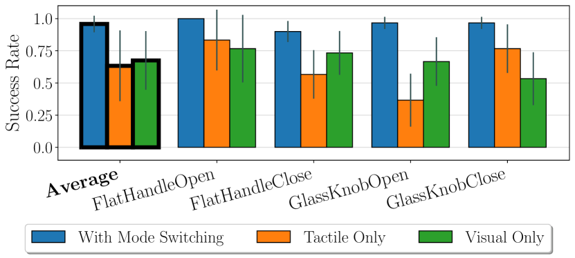
The see-through-your-skin visuotactile sensor used for this work is a relatively new concept, and while there is a clear intuitive understanding of its potential benefit [5, 17], its application to real-world tasks has been limited. In the interest of better understanding how mode switching, and how our policy mode switch output, can benefit performance on a real door opening task, we collected replays of demonstrations both with and without mode switching enabled. Specifically, we have three configurations: mode switching enabled, tactile-only (the sensor lights are always on), and visual-only (the sensor lights are always off). Given the clear benefit of including force matching shown in Section IV-D, and to isolate the benefits of mode switching, we included force matching in all three configurations. Also matching our experimental design in Section IV-D, we included all three sensing modalities (wrist-mounted eye-in-hand RGB images, STS images, and relative positions) in each mode switching configuration. The results of these tests are shown in Fig. 12, with the same training and testing parameters as described in Section IV-B.
Averaging the success rates of visual-only and tactile-only results together, the use of mode-switching results in an absolute task-average performance gain of 30.4%. Again, as with force matching, there are some task-specific patterns. The task-specific correlation is similar to our results comparing all components of the system simultaneously (Section IV-C): specifically, the performance gain for GlassKnob tasks is 38.3%, while the performance gain for FlatHandle tasks is only 22.5%. Given that this pattern does not occur in our force matching testing results, our results indicate that the GlassKnob policies gain more benefit from the use of the STS as a policy input (and, thus, are further harmed by the exclusion of mode switching). This is perhaps unsurprising, given that the handle requires less precision in the approach to properly grip and maintain contact.
As stated, another question that we were interested in answering is whether an STS sensor is beneficial as a policy input for door tasks, compared with using a more standard wrist-mounted eye-in-hand camera alone. The results from this section could imply that the wrist-mounted eye-in-hand camera alone cannot effectively solve these tasks. If it could, one may expect the network to learn to ignore the STS input data and have the same performance both with and without mode switching. The results in this section seem to indicate that the network is not capable of doing this, which suggests that either our network is not capable of learning this ability to “ignore” unhelpful data, or that indeed, the wrist camera alone cannot solve the tasks. While there is significant work that explores the former as being a general problem with neural network learning [47], our further exploration of this question in Section IV-F provides more evidence that the latter is likely to be the true explanation.
IV-E1 Mode Switching Trajectory Comparison
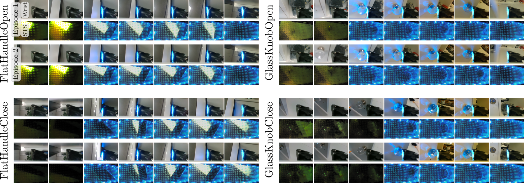
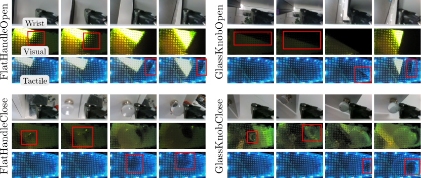
We can qualitatively verify the efficacy of mode switching established by Section IV-E directly comparing the visual-only and tactile-only STS data from replays of the same original demonstration. Fig. 13 shows visual-only and tactile-only data for replays of the same trajectory (along with the corresponding wrist camera data, for reference). Through observation, it is clear that the tactile-only data provides no information before contact is made with the handle or knob, while visual-only data provides poor tactile information during contact.
IV-E2 Mode Switching Timing Analysis
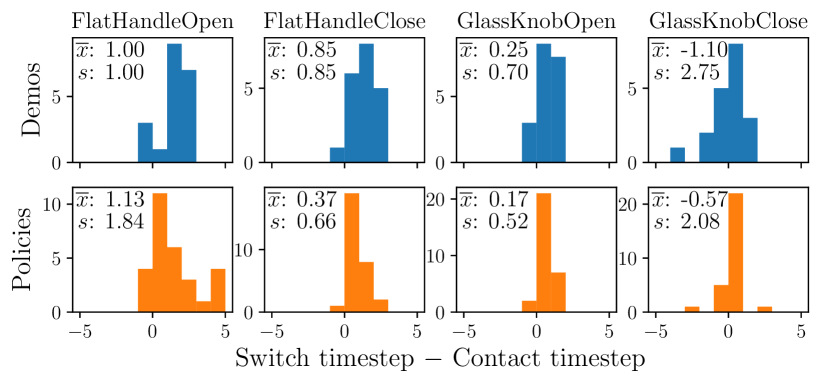
To better understand the quality of our learned mode switching policy output, we completed an analysis to evaluate the timing of the learned mode switch action compared with the expert labels. As described in Section III-G, an expert demonstrator may have a preference for having the sensor switch modes slightly before or after contact occurs, but for this analysis, we will consider that an optimal switch occurs at the moment of contact.
For each dataset with force matching, mode switching, and all three sensing modalities, we manually annotated each episode with the timestep at which contact was made between the handle/knob and the surface of the STS, and compared that to the timestep that the demonstrator provided a mode switch action label. The histograms of these timestep differences are shown in the top row of Fig. 14. While there are arguably certain task-specific patterns, such as a slightly higher timestep difference average for the handle tasks, the clearest pattern is that the mode switch label typically occurs within one timestep (0.1s) of contact being made. The bottom row shows the same analysis, but for autonomous policies. With the exception of a few outliers (particularly in FlatHandleOpen), the policies have converged to be closer to an average of zero timesteps between contact and mode switching, smoothing out the reactive/predictive timing errors from the expert dataset. The outliers in Flat Handle are mostly due to a causal mismatch, where occasionally the policy learns to switch modes based on when the arm starts opening the handle, instead of at the moment of contact [48].
IV-F Observation Space Study
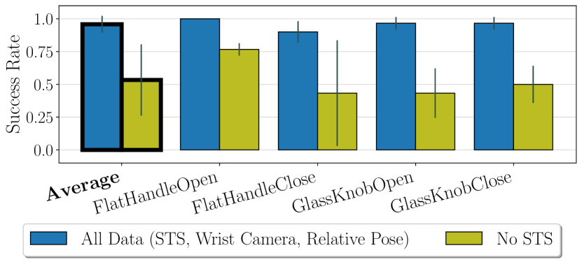
The third experimental question we hoped to answer was whether our door manipulation tasks can be solved with a wrist-mounted eye-in-hand camera alone, and whether the inclusion of STS data improves performance. To answer this question, we trained and tested policies with wrist RGB data and without STS data. To complete these tests, we did not need to collect any new human demonstration data or even any new replay data, instead just selectively excluding observations used for training the policies in Section IV-D and Section IV-E. All policies for these tests were trained with force matching enabled, given the clear benefits of both additions described in Section IV-D. Our policies with STS data included mode switching, given the benefits shown in Section IV-E. For policies excluding STS data, the STS sensor was set to visual-only, since the wrist camera is capable of observing the lighting change of the STS, which would hypothetically provide contact information as a cue.
The results of these tests are shown in Fig. 15. Adding an STS as input results in an average across-task increase in performance of 42.5%. It is worth reiterating that this performance gain only corresponds to the case where STS data is excluded as an input into the policy; the STS itself is still used indirectly for these policies through the use of force matching during collection of demonstrations. Without force matching, the performance gain over the baseline is 64.2% (as shown in Section IV-C), indicating that force matching alone provides some benefit, but the STS as a policy input is still quite valuable. One could use Eq. 6 directly with another means of sensing forces to achieve force matching, so these results can be described as a simulation of a version of our method with STS-free force matching and exclusively wrist-mounted eye-in-hand visual sensing. Once again, the average performance gain of 50% for the GlassKnob policies is higher than 35% for the FlatHandle policies, again demonstrating that the utility of the STS as a policy input is partially task-dependent.
IV-F1 Contribution of Relative Pose Input
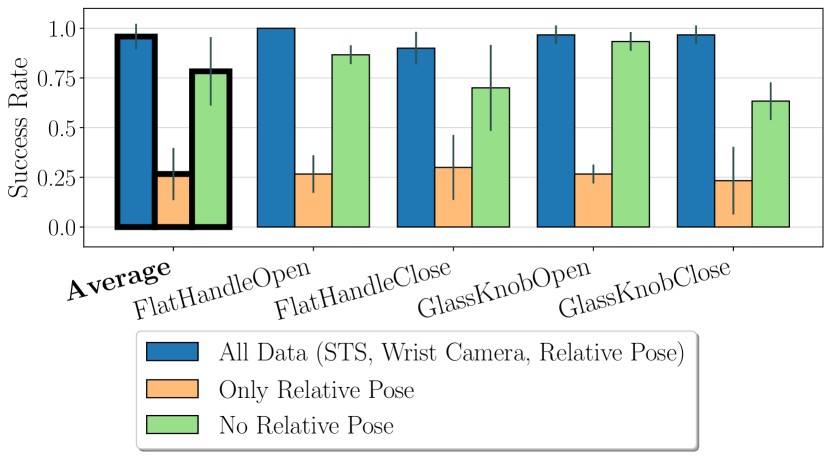
A natural followup question, and one which is not answered by any of our results thus far, is what the contribution of the relative pose data as a policy input is. As a reminder, there are three policy inputs that we investigated: STS images, wrist camera images, and numerical relative poses. Tasks with minimal variation in initial conditions can potentially be solved, at least partially, without access to visual information. To better understand the value of relative poses as inputs, we trained policies with and without relative pose as an input, as well as policies with only relative pose as an input. All other information regarding force matching and mode switching matches the description above in Section IV-F. The results of training and testing these three configurations are shown in Fig. 16.
We include relative pose alone as a baseline to show that, due to the initial randomization described in Section IV-A, the tasks require visual feedback to succeed consistently, and that a single “average” trajectory combined with impedance control is not, by itself, effective. The perhaps surprisingly relatively high performance of policies excluding relative pose shows that the visual data alone can provide information to solve the task fairly often. However, providing relative pose still allows for an average across-task policy improvement of 17.5% when including both wrist and STS data.
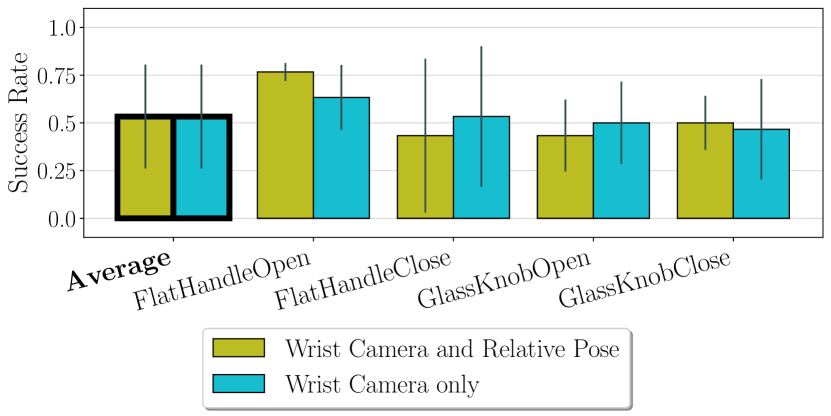
We also present the results of this comparison for policies excluding STS data in Fig. 17. The clear benefit of including relative pose shown in Fig. 16 is not exhibited when using eye-in-hand wrist camera data only. This result does not necessarily have a single explanation, but it does indicate that further study of the inclusion of numerical observation data is warranted in imitation learning, since prior work has shown it to have both a strictly positive [30, 8] and strictly negative [29] effect.
IV-G STS-Only Policy Performance
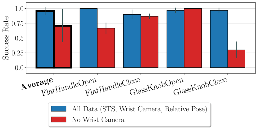
The inclusion of a wrist-mounted eye-in-hand camera is common for robotic manipulation, but many robotic configurations choose to exclude it. A related experimental question concerns whether an STS camera alone can be used to complete these challenging door manipulation tasks. From a practical perspective, this could slightly reduce the size and cost of a robotic installation. Furthermore, previous work has shown that simply adding more sensing to learned models does not always lead to improved performance [20, 29]. For this reason, in this section, we train several policies without using data from the wrist-mounted eye-in-hand camera, and compare performance to our previous results. First, we show results comparing training policies including force matching and mode switching both with and without the wrist camera in Fig. 18.
The results show an average across-task absolute performance increase of 25.0% when including the wrist camera. Notably, the performance improvement shows a large task-based discrepancy, with no improvement shown in FlatHandleClose and GlassKnobOpen, but a dramatic improvement in GlassKnobClose. This is at least partially because the initial reach in GlassKnobClose is more difficult than for any of the other tasks, and the wrist camera unquestionably helps provide clearer information for this task in particular (see Fig. 13 for visualization of STS visual data compared with wrist camera data for this task). Another conclusion from these results is that using exclusively the STS and relative pose (Fig. 18, red) as policy inputs results in a 17.5% higher success rate than using exclusively the wrist camera and relative pose (Fig. 15, light green). This finding requires further investigation with a larger variety of tasks, but indicates that contact-rich door tasks may get more benefit from a multimodal STS sensor alone than from a wrist camera alone.
IV-G1 Mode Switching Performance (STS-only)
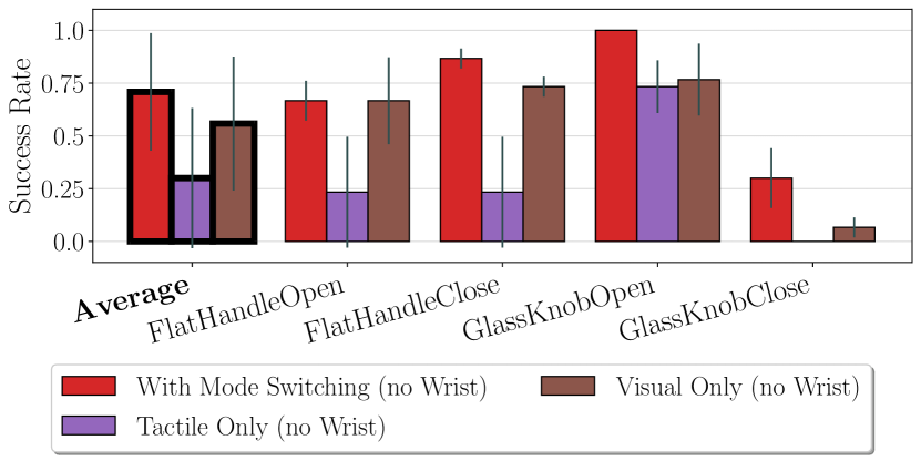
To further explore the use of policies with STS-only data, we also completed experiments where we evaluated the benefits of our policy mode switching output, replicating the experiments in Section IV-E, but excluding the eye-in-hand wrist camera. Specifically, we trained and tested policies using STS data in three configurations: with mode switching enabled, with the STS mode fixed to visual, and with the mode fixed to tactile. As in Section IV-E, we kept force matching enabled for all three configurations to isolate the effect of including mode switching, and we include relative poses as policy inputs for all policies.
The results of testing these policies are shown in Fig. 19. The performance increase of including mode switching with STS-only policies, averaging the across-task performance gain of both visual-only and tactile-only combined, is 27.9%, which is comparable to the increase of 30.4% shown in Section IV-E, when wrist camera data is included.
One striking difference from Section IV-E is the performance increase of mode switching over tactile-only policies of 40.8%, compared with only a 15.0% increase over visual-only policies. This is unsurprising, given that the tasks require a degree of reaching to make adequate contact with the handle or knob, and with both visual STS data and eye-in-hand wrist data removed, the tasks become far more challenging. The performance of tactile-only policies only matches visual-only for GlassKnobOpen, which can partially be explained by the fact that, even in tactile mode, the glass knob faintly shows up in the sensor images for this task (see Fig. 20). This is caused by a combination of external lighting factors and our removal of the top layer of the STS sensor (see Section IV-A), but the benefit does not appear in all tasks. Even in GlassKnobOpen, mode switching is clearly the optimal configuration in which to use the STS.

IV-G2 Contribution of Relative Pose Input (STS-only)
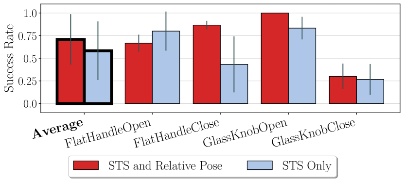
As a comparison with the effect of including relative positions as in input to policies with wrist camera data only (see Section IV-F1), we also completed similar experiments for policies with only STS data. The results in Fig. 21 compare testing results for policies with both STS and relative position data, only STS data, and only relative position data as inputs. In comparison with the results from Section IV-F1, there is an average performance increase of 12.5% when using relative poses with STS compared to the STS alone. However, the gain is not as significant as one may expect, once again reiterating that deeper study on the benefits of including numerical observation data for policies learned with imitation learning is warranted.
IV-H Expert Data Scaling
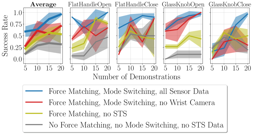
In our final set of experiments, we choose our most representative configurations from the preceding sections and train and test policies with 5, 10, and 15 expert trajectories (compared with 20 for all of our previous experiments). Fig. 22 shows the results of experiments with lower amounts of training data for these configurations. Most methods improve with increased data, but there are exceptions. For example, both STS-free methods do not improve significantly with increasing data for Flat Handle Close, Glass Knob, or Glass Knob Close, indicating that the eye-in-hand wrist camera doesn’t provide enough information to complete the task alone, regardless of data quantity. Conversely, eye-in-finger visual data, as well as tactile data, do contain sufficient information for these three tasks, so their performance scales with increasing data. A surprising finding is that for FlatHandleOpen, FlatHandleClose, and GlassKnobOpen, performance is quite good with force matching, mode switching, and all sensing modalities, even with only five demonstrations, though there is still a gradual increase in performance with more data. Performance on our hardest task, GlassKnobClose, clearly increases with more data, but the STS alone is not enough for this task. The performance of the two configurations that exclude STS input data both seem to plateau at 15 demonstrations, indicating that these tasks may be simply not possible to complete without the STS as an input, even with increasing data. It is possible that performance with a small number of demonstrations could be made even higher by deliberately selecting initial conditions that better cover the initial state distribution, but we did not explore that strategy in this work.
V Limitations
In this section, we discuss some limitations of our work. Although we used a single sensor for all of our experiments, the gel-based contact surface of the STS physically degrades over time. This limitation partially motivates the use of learned models for gel-based sensors; if sensor data changes marginally due to degradation, a practitioner can merely add more data to the dataset and retrain the policy. As well, the STS uses a standard visual camera, so policies trained on its data are susceptible to the same problems as other visual data paired with neural networks, such as overfitting to specific lighting conditions. Additionally, our initial state distribution (the randomization of the initial end-effector pose) is a design choice, so it may not represent a true distribution for, e.g., a mobile platform in a larger environment. Our policies are inherently single-task, though it is possible that training a single policy on all of our data could handle a variety of tasks. Finally, our force-matched replayed demonstrations still occasionally fail because both our method for measuring forces as well as our Cartesian impedance controller can suffer from accuracy issues, but both of these limitations can be improved with further tuning.
VI Conclusion
We presented a robotic imitation learning system that leverages a see-through-your-skin (STS) visuotactile sensor both as a measurement device to improve demonstration quality and as a multimodal source of dense data to learn from. Our first contribution was a system for force matching that used the STS in its tactile mode to measure a signal linearly related to force, which was subsequently used to improve demonstration quality through force-matched replays that better recreate the demonstrator’s force profile. Our second contribution was a demonstration of a learned approach to STS mode switching, in which a policy output is added to switch the sensor mode, and the labels are convenient provided by the demonstrator during demonstration replays. Our final contribution was a thorough observational study in which we compared and contrasted the value of the STS visuotactile data (in mode-switching, visual-only, and tactile-only configurations) with using an eye-in-hand wrist-mounted camera. We completed this study, as well as evaluation of our force matching and learned mode switching contributions, on four challenging contact-rich door opening and closing tasks with a real manipulator. We found that the inclusion of force matching, STS mode switching, and visuotactile data from an STS sensor as a policy input each increased policy success rates by 62.5%, 30.4%, and 42.5%, respectively. Potential directions for future work include improving the accuracy of our force sensing method or adding a means for self-improvement by detecting execution failures.
References
- [1] C. Chi, X. Sun, N. Xue, T. Li, and C. Liu, “Recent Progress in Technologies for Tactile Sensors,” Sensors, vol. 18, no. 4, p. 948, Apr. 2018.
- [2] W. Yuan, S. Dong, and E. H. Adelson, “GelSight: High-Resolution Robot Tactile Sensors for Estimating Geometry and Force,” Sensors, vol. 17, no. 12, p. 2762, Dec. 2017.
- [3] A. Padmanabha, F. Ebert, S. Tian, R. Calandra, C. Finn, and S. Levine, “OmniTact: A Multi-Directional High-Resolution Touch Sensor,” in 2020 IEEE International Conference on Robotics and Automation (ICRA), May 2020, pp. 618–624.
- [4] D. Ma, E. Donlon, S. Dong, and A. Rodriguez, “Dense Tactile Force Estimation using GelSlim and inverse FEM,” in 2019 International Conference on Robotics and Automation (ICRA), May 2019, pp. 5418–5424.
- [5] F. R. Hogan, M. Jenkin, S. Rezaei-Shoshtari, Y. Girdhar, D. Meger, and G. Dudek, “Seeing Through your Skin: Recognizing Objects with a Novel Visuotactile Sensor,” Dec. 2020.
- [6] F. R. Hogan, J.-F. Tremblay, B. H. Baghi, M. Jenkin, K. Siddiqi, and G. Dudek, “Finger-STS: Combined Proximity and Tactile Sensing for Robotic Manipulation,” IEEE Robotics and Automation Letters, vol. 7, no. 4, pp. 10 865–10 872, Oct. 2022.
- [7] A. G. Billard, S. Calinon, and R. Dillmann, “Learning from Humans,” in Springer Handbook of Robotics, B. Siciliano and O. Khatib, Eds. Cham: Springer International Publishing, 2016, pp. 1995–2014.
- [8] T. Ablett, Y. Zhai, and J. Kelly, “Seeing All the Angles: Learning Multiview Manipulation Policies for Contact-Rich Tasks from Demonstrations,” in Proceedings of the IEEE/RSJ International Conference on Intelligent Robots and Systems (IROS’21), Prague, Czech Republic, Sept. 2021.
- [9] K. Li, D. Chappell, and N. Rojas, “Immersive Demonstrations are the Key to Imitation Learning,” Jan. 2023.
- [10] A. Pervez, A. Ali, J.-H. Ryu, and D. Lee, “Novel learning from demonstration approach for repetitive teleoperation tasks,” in 2017 IEEE World Haptics Conference (WHC). Munich, Germany: IEEE, June 2017, pp. 60–65.
- [11] K. Fischer, et al., “A comparison of types of robot control for programming by Demonstration,” in 2016 11th ACM/IEEE International Conference on Human-Robot Interaction (HRI), Mar. 2016, pp. 213–220.
- [12] B. Akgun and K. Subramanian, “Robot Learning from Demonstration: Kinesthetic Teaching vs. Teleoperation,” Technical Report, 2011.
- [13] B. Siciliano, “Force Control,” in Robotics: Modelling, Planning and Control, ser. Advanced Textbooks in Control and Signal Processing, L. Sciavicco, L. Villani, and G. Oriolo, Eds. London: Springer, 2009, pp. 363–405.
- [14] M. H. Raibert and J. J. Craig, “Hybrid Position/Force Control of Manipulators,” Journal of Dynamic Systems, Measurement, and Control, vol. 103, no. 2, pp. 126–133, June 1981.
- [15] N. Hogan, “Impedance Control: An Approach to Manipulation,” in 1984 American Control Conference, June 1984, pp. 304–313.
- [16] A. Jilani, “Direct Shape from Touch Sensing,” Master’s Thesis [in Progress], McGill University, Jan. 2024.
- [17] A. Yamaguchi and C. G. Atkeson, “Implementing tactile behaviors using FingerVision,” in 2017 IEEE-RAS 17th International Conference on Humanoid Robotics (Humanoids), Nov. 2017, pp. 241–248.
- [18] A. M. Okamura, “Haptic Feedback in Robot-Assisted Minimally Invasive Surgery,” Current opinion in urology, vol. 19, no. 1, pp. 102–107, Jan. 2009.
- [19] O. Limoyo, T. Ablett, and J. Kelly, “Learning Sequential Latent Variable Models from Multimodal Time Series Data,” in Intelligent Autonomous Systems 17, ser. Lecture Notes in Networks and Systems, I. Petrovic, E. Menegatti, and I. Marković, Eds. Cham: Springer Nature Switzerland, 2023, pp. 511–528.
- [20] J. Hansen, F. Hogan, D. Rivkin, D. Meger, M. Jenkin, and G. Dudek, “Visuotactile-RL: Learning Multimodal Manipulation Policies with Deep Reinforcement Learning,” in 2022 International Conference on Robotics and Automation (ICRA), May 2022, pp. 8298–8304.
- [21] H. Li, et al., “See, Hear, and Feel: Smart Sensory Fusion for Robotic Manipulation,” in 6th Annual Conference on Robot Learning, Nov. 2022.
- [22] Y. Lin, J. Lloyd, A. Church, and N. F. Lepora, “Tactile Gym 2.0: Sim-to-Real Deep Reinforcement Learning for Comparing Low-Cost High-Resolution Robot Touch,” IEEE Robotics and Automation Letters, vol. 7, no. 4, pp. 10 754–10 761, Oct. 2022.
- [23] Y. She, S. Wang, S. Dong, N. Sunil, A. Rodriguez, and E. Adelson, “Cable manipulation with a tactile-reactive gripper,” The International Journal of Robotics Research, vol. 40, no. 12-14, pp. 1385–1401, Dec. 2021.
- [24] L. Villani and J. De Schutter, “Force Control,” in Springer Handbook of Robotics, ser. Springer Handbooks, B. Siciliano and O. Khatib, Eds. Cham: Springer International Publishing, 2016, pp. 195–220.
- [25] W. Yuan, “Tactile Measurement with a GelSight Sensor,” Master’s thesis, Massachusetts Institute of Technology, 2014.
- [26] W. Kim, W. D. Kim, J.-J. Kim, C.-H. Kim, and J. Kim, “UVtac: Switchable UV Marker-Based Tactile Sensing Finger for Effective Force Estimation and Object Localization,” IEEE Robotics and Automation Letters, vol. 7, no. 3, pp. 6036–6043, July 2022.
- [27] M. Bain and C. Sammut, “A Framework for Behavioural Cloning,” in Machine Intelligence 15. Oxford University Press, 1996, pp. 103–129.
- [28] P. Abbeel and A. Y. Ng, “Apprenticeship learning via inverse reinforcement learning,” in International Conference on Machine Learning (ICML’04). Banff, Alberta, Canada: ACM Press, 2004.
- [29] A. Mandlekar, et al., “What Matters in Learning from Offline Human Demonstrations for Robot Manipulation,” in Conference on Robot Learning, Nov. 2021.
- [30] T. Zhang, et al., “Deep Imitation Learning for Complex Manipulation Tasks from Virtual Reality Teleoperation,” in Proceedings of the IEEE International Conference on Robotics and Automation (ICRA’18). Brisbane, QLD, Australia: IEEE, May 2018, pp. 5628–5635.
- [31] T. Ablett, B. Chan, and J. Kelly, “Learning From Guided Play: Improving Exploration for Adversarial Imitation Learning With Simple Auxiliary Tasks,” IEEE Robotics and Automation Letters, vol. 8, no. 3, pp. 1263–1270, Mar. 2023.
- [32] W.-D. Chang, S. Fujimoto, D. Meger, and G. Dudek, “Imitation Learning from Observation through Optimal Transport,” Oct. 2023.
- [33] M. Orsini, et al., “What Matters for Adversarial Imitation Learning?” in Conference on Neural Information Processing Systems, June 2021.
- [34] P. Kormushev, S. Calinon, and D. G. Caldwell, “Imitation Learning of Positional and Force Skills Demonstrated via Kinesthetic Teaching and Haptic Input,” Advanced Robotics, vol. 25, no. 5, pp. 581–603, Jan. 2011.
- [35] Y. Chebotar, O. Kroemer, and J. Peters, “Learning robot tactile sensing for object manipulation,” in 2014 IEEE/RSJ International Conference on Intelligent Robots and Systems, Sept. 2014, pp. 3368–3375.
- [36] I. Huang and R. Bajcsy, “Robot Learning from Demonstration with Tactile Signals for Geometry-Dependent Tasks,” in 2020 IEEE/RSJ International Conference on Intelligent Robots and Systems (IROS). Las Vegas, NV, USA: IEEE, Oct. 2020, pp. 8323–8328.
- [37] S. Dasari, et al., “RB2: Robotic Manipulation Benchmarking with a Twist,” in Thirty-Fifth Conference on Neural Information Processing Systems Datasets and Benchmarks Track (Round 2), Oct. 2021.
- [38] Y. Wang, N. Figueroa, S. Li, A. Shah, and J. Shah, “Temporal Logic Imitation: Learning Plan-Satisficing Motion Policies from Demonstrations,” in 6th Annual Conference on Robot Learning, Aug. 2022.
- [39] N. Figueroa, “Easy-kinesthetic-recording,” https://github.com/nbfigueroa/easy-kinesthetic-recording, Oct. 2023.
- [40] G. Bradski, “The OpenCV library,” Dr. Dobb’s Journal of Software Tools, 2000.
- [41] R. Tsai and R. Lenz, “A new technique for fully autonomous and efficient 3D robotics hand/eye calibration,” IEEE Transactions on Robotics and Automation, vol. 5, no. 3, pp. 345–358, June 1989.
- [42] O. Limoyo, T. Ablett, F. Marić, L. Volpatti, and J. Kelly, “Self-Calibration of Mobile Manipulator Kinematic and Sensor Extrinsic Parameters Through Contact-Based Interaction,” in 2018 IEEE International Conference on Robotics and Automation (ICRA), May 2018, pp. 1–8.
- [43] A. Gupta, et al., “Reset-Free Reinforcement Learning via Multi-Task Learning: Learning Dexterous Manipulation Behaviors without Human Intervention,” in Proceedings of the 2021 IEEE International Conference on Robotics and Automation (ICRA’21), Apr. 2021.
- [44] Y. Lin, A. S. Wang, G. Sutanto, A. Rai, and F. Meier, “Polymetis,” https://facebookresearch.github.io/fairo/polymetis/, 2021.
- [45] S. Levine, C. Finn, T. Darrell, and P. Abbeel, “End-to-end training of deep visuomotor policies,” Journal of Machine Learning Research, vol. 17, no. 39, pp. 1–40, 2016.
- [46] K. He, X. Zhang, S. Ren, and J. Sun, “Deep Residual Learning for Image Recognition,” in Proceedings of the IEEE Conference on Computer Vision and Pattern Recognition (CVPR’16). Las Vegas, NV, USA: IEEE, June 2016, pp. 770–778.
- [47] O. Limoyo, B. Chan, F. Marić, B. Wagstaff, A. R. Mahmood, and J. Kelly, “Heteroscedastic Uncertainty for Robust Generative Latent Dynamics,” IEEE Robotics and Automation Letters, vol. 5, no. 4, pp. 6654–6661, Oct. 2020.
- [48] P. de Haan, D. Jayaraman, and S. Levine, “Causal Confusion in Imitation Learning,” arXiv:1905.11979 [cs, stat], Nov. 2019.
![[Uncaptioned image]](/html/2311.01248/assets/figs/headshots/trevor_outdoor_2023.jpg) |
Trevor Ablett received his Bachelor of Engineering in Mechatronics along with a Bachelor of Arts in Psychology from McMaster University, Hamilton, Canada in 2015. He is currently a Ph.D. Candidate in the Space and Terrestrial Autonomous Robotics (STARS) Laboratory at the University of Toronto Robotics Institute, Toronto, Canada and was previously an Applied Reinforcement Learning Research intern at the Samsung AI Centre in Montreal, Canada. His research interests include imitation and reinforcement learning, robotic manipulation, and improving the robustness and efficiency of learning-based robotics. |
![[Uncaptioned image]](/html/2311.01248/assets/figs/headshots/oliver_limoyo.jpeg) |
Oliver Limoyo received his B.Eng. degree in mechanical engineering from McGill University in 2016. He is currently pursuing a Ph.D. degree at the Space and Terrestrial Autonomous Robotic Systems (STARS) laboratory at the University of Toronto. His research interests include the integration of generative models for robotics, reinforcement learning and imitation learning. |
![[Uncaptioned image]](/html/2311.01248/assets/figs/headshots/adam_sigal.jpg) |
Adam Sigal received his BS from Université de Montréal in computer science in 2019, and his MEng in Electrical Engineering from McGill University in 2022. After graduating, he joined the Samsung AI Center in Montreal as a machine learning research engineer. His research has focused on autonomous robot navigation, human-robot interaction, robot manipulation with visuotactile feedback, and more recently, embodied applications of generative models. |
![[Uncaptioned image]](/html/2311.01248/assets/figs/headshots/affan_jilani.jpg) |
Affan Jilani received his Bachelor of Science degree in computer science from McGill University in 2020. He is currently pursing an M.Sc. degree at McGill University. His research interests are focused on solving computer vision problems, and include shape recovery and applications of computer vision for robotics. |
![[Uncaptioned image]](/html/2311.01248/assets/figs/headshots/jonathan_kelly.png) |
Jonathan Kelly received his Ph.D. degree in Computer Science from the University of Southern California, Los Angeles, USA, in 2011. From 2011 to 2013 he was a postdoctoral associate in the Computer Science and Artificial Intelligence Laboratory at the Massachusetts Institute of Technology, Cambridge, USA. He is currently an associate professor and director of the Space and Terrestrial Autonomous Robotic Systems (STARS) Laboratory at the University of Toronto Institute for Aerospace Studies, Toronto, Canada. Prof. Kelly holds the Tier II Canada Research Chair in Collaborative Robotics. His research interests include perception, planning, and learning for interactive robotic systems. |
![[Uncaptioned image]](/html/2311.01248/assets/figs/headshots/kaleem_siddiqi.jpg) |
Kaleem Siddiqi received his BS degree from Lafayette College in 1988 and his MS and PhD degrees from Brown University in 1990 and 1995, respectively, all in the field of electrical engineering. He is currently a Professor at the School of Computer Science at McGill University where he holds an FRQS Dual Chair in Health and Artificial Intelligence. He is also a member of McGill’s Centre for Intelligent Machines, an associate member of McGill’s Department of Mathematics and Statistics, MILA - the Québec AI Institute, and the Goodman Cancer Centre. He presently serves as Field Chief Editor of the journal Frontiers in Computer Science. Before moving to McGill in 1998, he was a postdoctoral associate in the Department of Computer Science at Yale University (1996-1998) and held a position in the Department of Electrical Engineering at McGill University (1995-1996). More recently he was also a visiting professor and consultant at the Samsung AI Centre in Montréal (2021-2023). His research interests are in computer vision, robotics, image analysis, biological shape, neuroscience and medical imaging. He is a member of Phi Beta Kappa, Tau Beta Pi, and Eta Kappa Nu. He is a senior member of the IEEE. |
![[Uncaptioned image]](/html/2311.01248/assets/figs/headshots/fhogan_headshot.jpg) |
Francois Hogan Francois Hogan received his B.S. and M.S. degrees in Mechanical Engineering from McGill University in 2013 and 2015 respectively. He received his Ph.D. in Mechanical Engineering from the Massachusetts Institute of Technology in 2019. Francois is currently a Senior AI Researcher at the Samsung AI Center in Montreal. His primary research focuses on exploiting tactile and visual feedback to enable robots to reliably manipulate their environment. Francois was a member of team MIT-Princeton’s 1st place finish 2017 at the Amazon Robotics Challenge’s Stowing task, is the recipient of the MIT Presidential Fellowship, was awarded the 2018 Amazon Robotics Best Systems Paper, and was a 2021 Finalist for Best Manipulation paper at ICRA 2020. |
![[Uncaptioned image]](/html/2311.01248/assets/figs/headshots/greg.jpg) |
Gregory Dudek is a professor and former director of the School of Computer Science at McGill Research Centre for Intelligent Machines (CIM), Research Director of Mobile Robotics Lab at McGill, and an Associate Member of the Dept. of Electrical Engineering. In 2008 he was made James McGill Chair. Since 2012 he has been the Scientific Director of the NSERC Canadian Field Robotics Network (NCFRN). He is the Lab Head and VP, Research of Samsung’s AI Center in Montreal. He has authored and co-authored over 300 research publications on subjects including visual object description, recognition, RF localization, robotic navigation and mapping, distributed system design, 5G telecommunications, and biological perception. This includes a book entitled “Computational Principles of Mobile Robotics” co-authored with Michael Jenkin and published by Cambridge University Press. He has chaired and been otherwise involved in numerous national and international conferences and professional activities concerned with Robotics, Machine Sensing and Computer Vision. His research interests include perception for mobile robotics, navigation and position estimation, environment and shape modelling, computational vision and collaborative filtering. |