Optimal Transport-Guided Conditional
Score-Based Diffusion Model

Xiang Gu1, Liwei Yang1, Jian Sun (✉)1,2,3, Zongben Xu1,2,3
1 School of Mathematics and Statistics, Xi’an Jiaotong University, Xi’an, China
2 Pazhou Laboratory (Huangpu), Guangzhou, China
3 Peng Cheng Laboratory, Shenzhen, China
{xianggu,yangliwei}@stu.xjtu.edu.cn {jiansun,zbxu}@xjtu.edu.cn
Abstract

Conditional score-based diffusion model (SBDM) is for conditional generation of target data with paired data as condition, and has achieved great success in image translation. However, it requires the paired data as condition, and there would be insufficient paired data provided in real-world applications. To tackle the applications with partially paired or even unpaired dataset, we propose a novel Optimal Transport-guided Conditional Score-based diffusion model (OTCS) in this paper. We build the coupling relationship for the unpaired or partially paired dataset based on L2subscript𝐿2L_{2}-regularized unsupervised or semi-supervised optimal transport, respectively. Based on the coupling relationship, we develop the objective for training the conditional score-based model for unpaired or partially paired settings, which is based on a reformulation and generalization of the conditional SBDM for paired setting. With the estimated coupling relationship, we effectively train the conditional score-based model by designing a “resampling-by-compatibility” strategy to choose the sampled data with high compatibility as guidance. Extensive experiments on unpaired super-resolution and semi-paired image-to-image translation demonstrated the effectiveness of the proposed OTCS model. From the viewpoint of optimal transport, OTCS provides an approach to transport data across distributions, which is a challenge for OT on large-scale datasets. We theoretically prove that OTCS realizes the data transport in OT with a theoretical bound. Code is available at https://github.com/XJTU-XGU/OTCS.

1 Introduction

Score-based diffusion models (SBDMs) [1, 2, 3, 4, 5, 6, 7, 8] have gained much attention in data generation. SBDMs perturb target data to a Gaussian noise by a diffusion process and learn the reverse process to transform the noise back to the target data. The conditional SBDMs [9, 2, 10, 11, 12, 13] that are conditioned on class labels, text, low-resolution images, etc., have shown great success in image generation and translation. The condition data and target data in the conditional SBDMs [9, 2, 10, 11, 12, 13] are often paired. That is, we are given a condition for each target sample in training, e.g., in the super-resolution [10, 14, 15], each high-resolution image (target data) in training is paired with its corresponding low-resolution image (condition). However, in real-world applications, there could not be sufficient paired training data, due to the labeling burden. Therefore, it is important and valuable to develop SBDMs for applications with only unpaired or partially paired training data, e.g., unpaired [16] or semi-paired [17] image-to-image translation (I2I). Though there are several SBDM-based approaches [18, 19, 20, 21, 22] for unpaired I2I, the score-based models in these approaches are often unconditioned, and the conditions are imposed in inference by cycle consistency [21], designing the initial states [19, 22], or adding a guidance term to the output of the unconditional score-based model [18, 20]. It is unclear how to train the conditional score-based model with unpaired training dataset. For the task with a few paired and a large number of unpaired data, i.e., partially paired dataset, there are few SBDMs for tackling this task, to the best of our knowledge.

This paper works on how to train the conditional score-based model with unpaired or partially paired training dataset. We consider the I2I applications in this paper where the condition data and target data are images respectively from different domains. The main challenges for this task are: 1) the lack of the coupling relationship between condition data and target data hinders the training of the conditional score-based model, and 2) it is unclear how to train the conditional score-based model even with an estimated coupling relationship, because it may not explicitly provide condition-target data pairs as in the setting with paired data. We propose a novel Optimal Transport-guided Conditional Score-based diffusion model (OTCS) to address these challenges. Note that different from the existing OT-related SBDMs that aim to understand [23] or promote [24, 25] the unconditional score-based models, our approach aims to develop the conditional score-based model for unpaired or partially paired data settings guided by OT.

We tackle the first challenge based on optimal transport (OT). Specifically, for applications with unpaired setting, e.g., unpaired super-resolution, practitioners often attempt to translate the condition data (e.g., low-resolution images) to target domain (e.g., consisting of high-resolution images) while preserving image structures [26], etc. We handle this task using unsupervised OT [27] that transports data points across distributions with the minimum transport cost. The coupling relationship of condition data and target data is modeled in the transport plan of unsupervised OT. For applications with partially paired setting, it is reasonable to utilize the paired data to guide building the coupling relationship of unpaired data, because the paired data annotated by humans should have a reliable coupling relationship. The semi-supervised OT [28] is dedicated to leveraging the annotated keypoint pairs to guide the matching of the other data points. So we build the coupling relationship for partially paired dataset using semi-supervised OT by taking the paired data as keypoints.

To tackle the second challenge, we first provide a reformulation of the conditional SBDM for paired setting, in which the coupling relationship of paired data is explicitly considered. Meanwhile, the coupling relationship in this reformulation is closely related to the formulation of the coupling from L2subscript𝐿2L_{2}-regularized OT. This enables us to generalize the objective of the conditional SBDM for paired setting to unpaired and partially paired settings based on OT. To train the conditional score-based model using mini-batch data, directly applying the standard training algorithms to our approach can lead to sub-optimal performance of the trained conditional score-based model. To handle this challenge, we propose a new “resampling-by-compatibility” strategy to choose sampled data with high compatibility as guidance in training, which shows effectiveness in experiments.

We conduct extensive experiments on unpaired super-resolution and semi-paired I2I tasks, showing the effectiveness of the proposed OTCS for both applications with unpaired and partially paired settings. From the viewpoint of OT, the proposed OTCS offers an approach to transport the data points across distributions, which is known as a challenging problem in OT on large-scale datasets. The data transport in our approach is realized by generating target samples from the optimal conditional transport plan given a source sample, leveraging the capability of SBDMs for data generation. Theoretically and empirically, we show that OTCS can generate samples from the optimal conditional transport plan of the L2subscript𝐿2L_{2}-regularized unsupervised or semi-supervised OTs.

2 Background

Our method is closely related to OT and conditional SBDMs, which will be introduced below.

2.1 Conditional SBDMs with Paired Data

The conditional SBDMs [9, 2, 10, 11, 12, 6, 13] aim to generate a target sample 𝐲𝐲\mathbf{y} from the distribution q𝑞q of target training data given a condition data 𝐱𝐱\mathbf{x}. For the paired setting, each target training sample 𝐲𝐲\mathbf{y} is paired with a condition data 𝐱cond(𝐲)subscript𝐱cond𝐲\mathbf{x}_{\rm cond}(\mathbf{y}). The conditional SBDMs with paired dataset can be roughly categorized into two types, respectively under the classifier guidance [6] and classifier-free guidance [9, 2, 10, 11, 12, 13]. Our approach is mainly related to the second type of methods. These methods use a forward stochastic differential equation (SDE) to add Gaussian noises to the target training data for training the conditional score-based model. The forward SDE is d𝐲t=f(𝐲t,t)dt+g(t)d𝐰 with 𝐲0qdsubscript𝐲𝑡𝑓subscript𝐲𝑡𝑡d𝑡𝑔𝑡d𝐰 with subscript𝐲0similar-to𝑞\mathop{}\!\mathrm{d}\mathbf{y}_{t}=f(\mathbf{y}_{t},t)\mathop{}\!\mathrm{d}t+g(t)\mathop{}\!\mathrm{d}\mathbf{w}\mbox{ with }\mathbf{y}_{0}\sim q, and t[0,T]𝑡0𝑇t\in[0,T], where 𝐰D𝐰superscript𝐷\mathbf{w}\in\mathbb{R}^{D} is a standard Wiener process, f(,t):DD:𝑓𝑡superscript𝐷superscript𝐷f(\cdot,t):\mathbb{R}^{D}\rightarrow\mathbb{R}^{D} is the drift coefficient, and g(t)𝑔𝑡g(t)\in\mathbb{R} is the diffusion coefficient. Let pt|0subscript𝑝conditional𝑡0p_{t|0} be the conditional distribution of 𝐲tsubscript𝐲𝑡\mathbf{y}_{t} given the initial state 𝐲0subscript𝐲0\mathbf{y}_{0}, and ptsubscript𝑝𝑡p_{t} be the marginal distribution of 𝐲tsubscript𝐲𝑡\mathbf{y}_{t}. We can choose the f(𝐲,t)𝑓𝐲𝑡f(\mathbf{y},t), g(t)𝑔𝑡g(t), and T𝑇T such that 𝐲tsubscript𝐲𝑡\mathbf{y}_{t} approaches some analytically tractable prior distribution pprior(𝐲T)subscript𝑝priorsubscript𝐲𝑇p_{\rm prior}(\mathbf{y}_{T}) at time t=T𝑡𝑇t=T, i.e., pT(𝐲T)pprior(𝐲T)subscript𝑝𝑇subscript𝐲𝑇subscript𝑝priorsubscript𝐲𝑇p_{T}(\mathbf{y}_{T})\approx p_{\rm{prior}}(\mathbf{y}_{T}). We take f,g,T𝑓𝑔𝑇f,g,T, and ppriorsubscript𝑝priorp_{\rm{prior}} from two popular SDEs, i.e., VE-SDE and VP-SDE [3] (please refer to Appendix A for model details). The conditional score-based model is trained by denoising score-matching loss:

𝒥DSM(θ)=𝔼twt𝔼𝐲0q𝔼𝐲tpt|0(𝐲t|𝐲0)sθ(𝐲t;𝐱cond(𝐲0),t)𝐲tlogpt|0(𝐲t|𝐲0)22,\mathcal{J}_{\rm DSM}(\theta)=\mathbb{E}_{t}w_{t}\mathbb{E}_{\mathbf{y}_{0}\sim q}\mathbb{E}_{\mathbf{y}_{t}\sim p_{t|0}(\mathbf{y}_{t}|\mathbf{y}_{0})}\left\|s_{\theta}(\mathbf{y}_{t};\mathbf{x}_{\rm cond}(\mathbf{y}_{0}),t)-\nabla_{\mathbf{y}_{t}}\log p_{t|0}(\mathbf{y}_{t}|\mathbf{y}_{0})\right\|_{2}^{2}, (1)

where wtsubscript𝑤𝑡w_{t} is the weight for time t𝑡t. In this paper, t𝑡t is uniformly sampled from [0,T]0𝑇[0,T], i.e., t𝒰([0,T])similar-to𝑡𝒰0𝑇t\sim\mathcal{U}([0,T]). With the trained sθ^(𝐲;𝐱,t)subscript𝑠^𝜃𝐲𝐱𝑡s_{\hat{\theta}}(\mathbf{y};\mathbf{x},t), given a condition data 𝐱𝐱\mathbf{x}, the target sample 𝐲0subscript𝐲0\mathbf{y}_{0} is generated by the reverse SDE as d𝐲t=[f(𝐲t,t)g(t)2sθ^(𝐲t;𝐱,t)]dt+g(t)d𝐰¯dsubscript𝐲𝑡delimited-[]𝑓subscript𝐲𝑡𝑡𝑔superscript𝑡2subscript𝑠^𝜃subscript𝐲𝑡𝐱𝑡d𝑡𝑔𝑡d¯𝐰\mathop{}\!\mathrm{d}\mathbf{y}_{t}=\left[f(\mathbf{y}_{t},t)-g(t)^{2}s_{\hat{\theta}}(\mathbf{y}_{t};\mathbf{x},t)\right]\mathop{}\!\mathrm{d}t+g(t)\mathop{}\!\mathrm{d}\bar{\mathbf{w}}, where 𝐰¯¯𝐰\bar{\mathbf{w}} is a standard Wiener process in the reverse-time direction. This process starts from a noise sample 𝐲Tsubscript𝐲𝑇\mathbf{y}_{T} and ends at t=0𝑡0t=0.

2.2 Optimal Transport

Unsupervised OT.

We consider a source distribution p𝑝p and a target distribution q𝑞q. The unsupervised OT [29] aims to find the optimal coupling/transport plan π𝜋\pi, i.e., a joint distribution of p𝑝p and q𝑞q, such that the transport cost is minimized, formulated as the following optimization problem:

minπΓ𝔼(𝐱,𝐲)πc(𝐱,𝐲), s.t. Γ={π:T#𝐱π=p,T#𝐲π=q},subscript𝜋Γsubscript𝔼similar-to𝐱𝐲𝜋𝑐𝐱𝐲 s.t. Γconditional-set𝜋formulae-sequencesuperscriptsubscript𝑇#𝐱𝜋𝑝superscriptsubscript𝑇#𝐲𝜋𝑞\min_{\pi\in\Gamma}\mathbb{E}_{(\mathbf{x},\mathbf{y})\sim\pi}c(\mathbf{x},\mathbf{y}),\mbox{ s.t. }\Gamma=\{\pi:T_{\#}^{\mathbf{x}}\pi=p,T_{\#}^{\mathbf{y}}\pi=q\}, (2)

where c𝑐c is the cost function. T#𝐱πsuperscriptsubscript𝑇#𝐱𝜋T_{\#}^{\mathbf{x}}\pi is the marginal distribution of π𝜋\pi w.r.t. random variable 𝐱𝐱\mathbf{x}. T#𝐱π=psuperscriptsubscript𝑇#𝐱𝜋𝑝T_{\#}^{\mathbf{x}}\pi=p means π(𝐱,𝐲)d𝐲=p(𝐱),𝐱𝒳formulae-sequence𝜋𝐱𝐲differential-d𝐲𝑝𝐱for-all𝐱𝒳\int\pi(\mathbf{x},\mathbf{y})\mathop{}\!\mathrm{d}\mathbf{y}=p(\mathbf{x}),\forall\mathbf{x}\in\mathcal{X}. Similarly, T#𝐲π=qsuperscriptsubscript𝑇#𝐲𝜋𝑞T_{\#}^{\mathbf{y}}\pi=q indicates π(𝐱,𝐲)d𝐱=q(𝐲),𝐲𝒴formulae-sequence𝜋𝐱𝐲differential-d𝐱𝑞𝐲for-all𝐲𝒴\int\pi(\mathbf{x},\mathbf{y})\mathop{}\!\mathrm{d}\mathbf{x}=q(\mathbf{y}),\forall\mathbf{y}\in\mathcal{Y}.

Semi-supervised OT.

The semi-supervised OT is pioneered by [28, 30]. In semi-supervised OT, a few matched pairs of source and target data points (called “keypoints”) 𝒦={(𝐱k,𝐲k)}k=1K𝒦superscriptsubscriptsubscript𝐱𝑘subscript𝐲𝑘𝑘1𝐾\mathcal{K}=\{(\mathbf{x}_{k},\mathbf{y}_{k})\}_{k=1}^{K} are given, where K𝐾K is the number of keypoint pairs. The semi-supervised OT aims to leverage the given matched keypoints to guide the correct transport in OT by preserving the relation of each data point to the keypoints. Mathematically, we have

minπ~Γ~𝔼(𝐱,𝐲)mπ~g(𝐱,𝐲), s.t. Γ~={π~:T#𝐱(mπ~)=p,T#𝐲(mπ~)=q},subscript~𝜋~Γsubscript𝔼similar-to𝐱𝐲tensor-product𝑚~𝜋𝑔𝐱𝐲 s.t. ~Γconditional-set~𝜋formulae-sequencesuperscriptsubscript𝑇#𝐱tensor-product𝑚~𝜋𝑝superscriptsubscript𝑇#𝐲tensor-product𝑚~𝜋𝑞\min_{\tilde{\pi}\in\tilde{\Gamma}}\mathbb{E}_{(\mathbf{x},\mathbf{y})\sim m\otimes\tilde{\pi}}g(\mathbf{x},\mathbf{y}),\mbox{ s.t. }\tilde{\Gamma}=\{\tilde{\pi}:T_{\#}^{\mathbf{x}}(m\otimes\tilde{\pi})=p,T_{\#}^{\mathbf{y}}(m\otimes\tilde{\pi})=q\}, (3)

where the transport plan mπ~tensor-product𝑚~𝜋m\otimes\tilde{\pi} is (mπ~)(𝐱,𝐲)=m(𝐱,𝐲)π~(𝐱,𝐲)tensor-product𝑚~𝜋𝐱𝐲𝑚𝐱𝐲~𝜋𝐱𝐲(m\otimes\tilde{\pi})(\mathbf{x},\mathbf{y})=m(\mathbf{x},\mathbf{y})\tilde{\pi}(\mathbf{x},\mathbf{y}), and m𝑚m is a binary mask function. Given a pair of keypoints (𝐱k0,𝐲k0)𝒦subscript𝐱subscript𝑘0subscript𝐲subscript𝑘0𝒦(\mathbf{x}_{k_{0}},\mathbf{y}_{k_{0}})\in\mathcal{K}, then m(𝐱k0,𝐲k0)=1𝑚subscript𝐱subscript𝑘0subscript𝐲subscript𝑘01m(\mathbf{x}_{k_{0}},\mathbf{y}_{k_{0}})=1, m(𝐱k0,𝐲)=0𝑚subscript𝐱subscript𝑘0𝐲0m(\mathbf{x}_{k_{0}},\mathbf{y})=0 for 𝐲𝐲k0𝐲subscript𝐲subscript𝑘0\mathbf{y}\neq\mathbf{y}_{k_{0}}, and m(𝐱,𝐲k0)=0𝑚𝐱subscript𝐲subscript𝑘00m(\mathbf{x},\mathbf{y}_{k_{0}})=0 for 𝐱𝐱k0𝐱subscript𝐱subscript𝑘0\mathbf{x}\neq\mathbf{x}_{k_{0}}. m(𝐱,𝐲)=1𝑚𝐱𝐲1m(\mathbf{x},\mathbf{y})=1 if 𝐱,𝐲𝐱𝐲\mathbf{x},\mathbf{y} do not coincide with any keypoint. The mask-based modeling of the transport plan ensures that the keypoint pairs are always matched in the derived transport plan. g𝑔g in Eq. (3) is defined as g(𝐱,𝐲)=d(R𝐱s,R𝐲t)𝑔𝐱𝐲𝑑subscriptsuperscript𝑅𝑠𝐱subscriptsuperscript𝑅𝑡𝐲g(\mathbf{x},\mathbf{y})=d(R^{s}_{\mathbf{x}},R^{t}_{\mathbf{y}}), where R𝐱s,R𝐲s(0,1)Ksubscriptsuperscript𝑅𝑠𝐱subscriptsuperscript𝑅𝑠𝐲superscript01𝐾R^{s}_{\mathbf{x}},R^{s}_{\mathbf{y}}\in(0,1)^{K} model the vector of relation of 𝐱𝐱\mathbf{x}, 𝐲𝐲\mathbf{y} to each of the paired keypoints in source and target domain respectively, and d𝑑d is the Jensen–Shannon divergence. The k𝑘k-th elements of R𝐱ssubscriptsuperscript𝑅𝑠𝐱R^{s}_{\mathbf{x}} and R𝐱ssubscriptsuperscript𝑅𝑠𝐱R^{s}_{\mathbf{x}} are respectively defined by

R𝐱,ks=exp(c(𝐱,𝐱k)/τ)l=1Kexp(c(𝐱,𝐱l)/τ), R𝐲,kt=exp(c(𝐲,𝐲k)/τ)l=1Kexp(c(𝐲,𝐲l)/τ),formulae-sequencesubscriptsuperscript𝑅𝑠𝐱𝑘𝑐𝐱subscript𝐱𝑘𝜏superscriptsubscript𝑙1𝐾𝑐𝐱subscript𝐱𝑙𝜏 subscriptsuperscript𝑅𝑡𝐲𝑘𝑐𝐲subscript𝐲𝑘𝜏superscriptsubscript𝑙1𝐾𝑐𝐲subscript𝐲𝑙𝜏R^{s}_{\mathbf{x},k}=\frac{\exp(-c(\mathbf{x},\mathbf{x}_{k})/\tau)}{\sum_{l=1}^{K}\exp(-c(\mathbf{x},\mathbf{x}_{l})/\tau)},\mbox{ }R^{t}_{\mathbf{y},k}=\frac{\exp(-c(\mathbf{y},\mathbf{y}_{k})/\tau)}{\sum_{l=1}^{K}\exp(-c(\mathbf{y},\mathbf{y}_{l})/\tau)}, (4)

where τ𝜏\tau is set to 0.1. Note that, to ensure feasible solutions, the mass of paired keypoints should be equal, i.e., p(𝐱k)=q(𝐲k),(𝐱k,𝐲k)𝒦formulae-sequence𝑝subscript𝐱𝑘𝑞subscript𝐲𝑘for-allsubscript𝐱𝑘subscript𝐲𝑘𝒦p(\mathbf{x}_{k})=q(\mathbf{y}_{k}),\forall(\mathbf{x}_{k},\mathbf{y}_{k})\in\mathcal{K}. Please refer to [28] for more details.

L2subscript𝐿2L_{2}-regularized unsupervised and semi-supervised OTs.

As in Eqs. (2) and (3), both the unsupervised and semi-supervised OTs are linear programs that are computationally expensive to solve for larger sizes of training datasets. Researchers then present the L2subscript𝐿2L_{2}-regularized versions of unsupervised and semi-supervised OTs that can be solved by training networks [31, 32]. The L2subscript𝐿2L_{2}-regularized unsupervised and semi-supervised OTs are respectively given by

minπΓ𝔼(𝐱,𝐲)πc(𝐱,𝐲)+ϵχ2(πp×q) and minπ~Γ~𝔼(𝐱,𝐲)mπ~g(𝐱,𝐲)+ϵχ2(mπ~p×q),subscript𝜋Γsubscript𝔼similar-to𝐱𝐲𝜋𝑐𝐱𝐲italic-ϵsuperscript𝜒2conditional𝜋𝑝𝑞 and subscript~𝜋~Γsubscript𝔼similar-to𝐱𝐲tensor-product𝑚~𝜋𝑔𝐱𝐲italic-ϵsuperscript𝜒2conditionaltensor-product𝑚~𝜋𝑝𝑞\min_{\pi\in\Gamma}{\mathbb{E}}_{(\mathbf{x},\mathbf{y})\sim\pi}c(\mathbf{x},\mathbf{y})+\epsilon\chi^{2}(\pi\|p\times q)\mbox{ and }\min_{\tilde{\pi}\in\tilde{\Gamma}}{\mathbb{E}}_{(\mathbf{x},\mathbf{y})\sim m\otimes\tilde{\pi}}g(\mathbf{x},\mathbf{y})+\epsilon\chi^{2}(m\otimes\tilde{\pi}\|p\times q), (5)

where χ2(πp×q)=π(𝐱,𝐲)2p(𝐱)q(𝐲)d𝐱d𝐲superscript𝜒2conditional𝜋𝑝𝑞𝜋superscript𝐱𝐲2𝑝𝐱𝑞𝐲differential-d𝐱differential-d𝐲\chi^{2}(\pi\|p\times q)=\int\frac{\pi(\mathbf{x},\mathbf{y})^{2}}{p(\mathbf{x})q(\mathbf{y})}\mathop{}\!\mathrm{d}\mathbf{x}\mathop{}\!\mathrm{d}\mathbf{y}, ϵitalic-ϵ\epsilon is regularization factor. The duality of the L2subscript𝐿2L_{2}-regularized unsupervised and semi-supervised OTs can be unified in the following formulation [31, 32]:

maxu,vOT(u,v)=𝔼𝐱pu(𝐱)+𝔼𝐲qv(𝐲)14ϵ𝔼𝐱p,𝐲qI(𝐱,𝐲)[(u(𝐱)+v(𝐲)ξ(𝐱,𝐲))+]2,subscript𝑢𝑣subscriptOT𝑢𝑣subscript𝔼similar-to𝐱𝑝𝑢𝐱subscript𝔼similar-to𝐲𝑞𝑣𝐲14italic-ϵsubscript𝔼formulae-sequencesimilar-to𝐱𝑝similar-to𝐲𝑞𝐼𝐱𝐲superscriptdelimited-[]subscript𝑢𝐱𝑣𝐲𝜉𝐱𝐲2\max_{u,v}\mathcal{F}_{\rm OT}(u,v)=\mathbb{E}_{\mathbf{x}\sim p}u(\mathbf{x})+\mathbb{E}_{\mathbf{y}\sim q}v(\mathbf{y})-\frac{1}{4\epsilon}\mathbb{E}_{\mathbf{x}\sim p,\mathbf{y}\sim q}I(\mathbf{x},\mathbf{y})\left[\left(u(\mathbf{x})+v(\mathbf{y})-\xi(\mathbf{x},\mathbf{y})\right)_{+}\right]^{2}, (6)

where a+=max(a,0)subscript𝑎𝑎0a_{+}=\max(a,0). For unsupervised OT, I(𝐱,𝐲)=1𝐼𝐱𝐲1I(\mathbf{x},\mathbf{y})=1 and ξ(𝐱,𝐲)=c(𝐱,𝐲)𝜉𝐱𝐲𝑐𝐱𝐲\xi(\mathbf{x},\mathbf{y})=c(\mathbf{x},\mathbf{y}). For semi-supervised OT, I(𝐱,𝐲)=m(𝐱,𝐲)𝐼𝐱𝐲𝑚𝐱𝐲I(\mathbf{x},\mathbf{y})=m(\mathbf{x},\mathbf{y}) and ξ(𝐱,𝐲)=g(𝐱,𝐲)𝜉𝐱𝐲𝑔𝐱𝐲\xi(\mathbf{x},\mathbf{y})=g(\mathbf{x},\mathbf{y}). In [31, 32], u,v𝑢𝑣u,v are represented by neural networks uω,vωsubscript𝑢𝜔subscript𝑣𝜔u_{\omega},v_{\omega} with parameters ω𝜔\omega that are trained by mini-batch-based stochastic optimization algorithms using the loss function in Eq. (6). The pseudo-code for training uω,vωsubscript𝑢𝜔subscript𝑣𝜔u_{\omega},v_{\omega} is given in Appendix A. Using the parameters ω^^𝜔{\hat{\omega}} after training, the estimate of optimal transport plan is

π^(𝐱,𝐲)=H(𝐱,𝐲)p(𝐱)q(𝐲), where H(𝐱,𝐲)=12ϵI(𝐱,𝐲)(uω^(𝐱)+vω^(𝐲)ξ(𝐱,𝐲))+.formulae-sequence^𝜋𝐱𝐲𝐻𝐱𝐲𝑝𝐱𝑞𝐲 where 𝐻𝐱𝐲12italic-ϵ𝐼𝐱𝐲subscriptsubscript𝑢^𝜔𝐱subscript𝑣^𝜔𝐲𝜉𝐱𝐲\hat{\pi}(\mathbf{x},\mathbf{y})=H(\mathbf{x},\mathbf{y})p(\mathbf{x})q(\mathbf{y}),\mbox{ where }H(\mathbf{x},\mathbf{y})=\frac{1}{2\epsilon}I(\mathbf{x},\mathbf{y})\left(u_{\hat{\omega}}(\mathbf{x})+v_{\hat{\omega}}(\mathbf{y})-\xi(\mathbf{x},\mathbf{y})\right)_{+}. (7)

H𝐻H is called compatibility function. Note that π^^𝜋\hat{\pi} and H𝐻H depend on c𝑐c and ϵitalic-ϵ\epsilon, which will be specified in experimental details in Appendix C.
Refer to caption
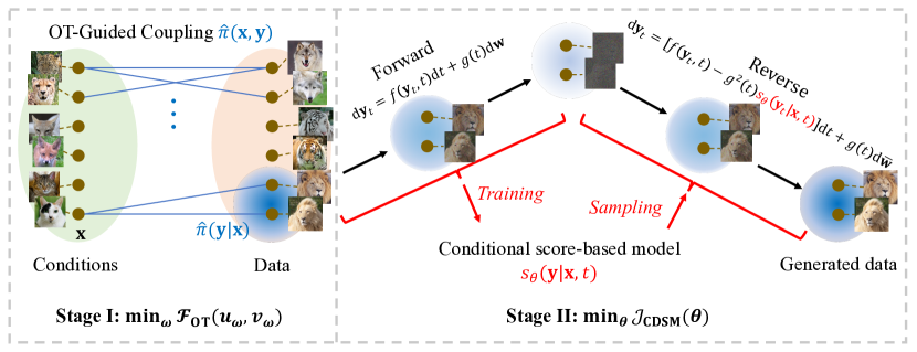
Figure 1: Illustation of optimal transport-guided conditional score-based diffusion model. We build the coupling π^(𝐱,𝐲)^𝜋𝐱𝐲\hat{\pi}(\mathbf{x},\mathbf{y}) of condition data (e.g., source images in I2I) 𝐱𝐱\mathbf{x} and target data 𝐲𝐲\mathbf{y} guided by OT. Based on the coupling, we train the conditional score-based model sθ(𝐲;𝐱,t)subscript𝑠𝜃𝐲𝐱𝑡s_{\theta}(\mathbf{y};\mathbf{x},t) by OT-guided conditional denoising score-matching that uses the forward SDE to diffuse target data to noise. With sθ(𝐲;𝐱,t)subscript𝑠𝜃𝐲𝐱𝑡s_{\theta}(\mathbf{y};\mathbf{x},t), we generate data given the condition 𝐱𝐱\mathbf{x} using the reverse SDE in inference.

3 OT-Guided Conditional SBDM

We aim to develop conditional SBDM for applications with unpaired or partially paired setting. The unpaired setting means that there is no paired condition data and target data in training. For example, in unpaired image-to-image translation (I2I), the source and target data in the training set are all unpaired. For the partially paired setting, along with the unpaired set of condition data (e.g., source data in I2I) and target data, we are also given a few paired condition data and target data.

We propose an Optimal Transport-guided Conditional SBDM, dubbed OTCS, for conditional diffusion in both unpaired and partially paired settings. The basic idea is illustrated in Fig. 1. Since the condition data and target data are not required to be paired in the training dataset, we build the coupling relationship of condition and target data using OT [27, 28]. Based on the estimated coupling, we propose the OT-guided conditional denoising score matching to train the conditional score-based model in the unpaired or partially paired setting. With the trained conditional score-based model, we generate a sample by the reverse SDE given the condition. We next elaborate on the motivations, OT-guided conditional denoising score matching, training, and inference of our approach.

3.1 Motivations for OT-Guided Conditional SBDM

We provide a reformulation for the conditional score-based model with paired training dataset discussed in Sect. 2.1, and this formulation motivates us to extend the conditional SBDM to unpaired and partially paired settings in Sect. 3.2. Let q𝑞q and p𝑝p respectively denote the distributions of target data and condition data. In the paired setting, we denote the condition data as 𝐱cond(𝐲)subscript𝐱cond𝐲\mathbf{x}_{\rm cond}(\mathbf{y}) for a target data 𝐲𝐲\mathbf{y}, and p𝑝p is the measure by push-forwarding q𝑞q using 𝐱condsubscript𝐱cond\mathbf{x}_{\rm cond} , i.e., p(𝐱)={𝐲:𝐱cond(𝐲)=𝐱}q(𝐲)𝑝𝐱subscriptconditional-set𝐲subscript𝐱cond𝐲𝐱𝑞𝐲p(\mathbf{x})=\sum_{\{\mathbf{y}:\mathbf{x}_{\rm cond}(\mathbf{y})=\mathbf{x}\}}q(\mathbf{y}) over the paired training dataset.

Proposition 1.

Let 𝒞(𝐱,𝐲)=1p(𝐱)δ(𝐱𝐱cond(𝐲))𝒞𝐱𝐲1𝑝𝐱𝛿𝐱subscript𝐱cond𝐲\mathcal{C}(\mathbf{x},\mathbf{y})=\frac{1}{p(\mathbf{x})}\delta(\mathbf{x}-\mathbf{x}_{\rm cond}(\mathbf{y})) where δ𝛿\delta is the Dirac delta function, then 𝒥DSM(θ)subscript𝒥DSM𝜃\mathcal{J}_{\rm DSM}(\theta) in Eq. (1) can be reformulated as

𝒥DSM(θ)=𝔼twt𝔼𝐱p𝔼𝐲q𝒞(𝐱,𝐲)𝔼𝐲tpt|0(𝐲t|𝐲)sθ(𝐲t;𝐱,t)𝐲tlogpt|0(𝐲t|𝐲)22.\mathcal{J}_{\rm DSM}(\theta)=\mathbb{E}_{t}w_{t}\mathbb{E}_{\mathbf{x}\sim p}\mathbb{E}_{\mathbf{y}\sim q}\mathcal{C}(\mathbf{x},\mathbf{y})\mathbb{E}_{\mathbf{y}_{t}\sim p_{t|0}(\mathbf{y}_{t}|\mathbf{y})}\left\|s_{\theta}(\mathbf{y}_{t};\mathbf{x},t)-\nabla_{\mathbf{y}_{t}}\log p_{t|0}(\mathbf{y}_{t}|\mathbf{y})\right\|_{2}^{2}. (8)

Furthermore, γ(𝐱,𝐲)=𝒞(𝐱,𝐲)p(𝐱)q(𝐲)𝛾𝐱𝐲𝒞𝐱𝐲𝑝𝐱𝑞𝐲\gamma(\mathbf{x},\mathbf{y})=\mathcal{C}(\mathbf{x},\mathbf{y})p(\mathbf{x})q(\mathbf{y}) is a joint distribution for marginal distributions p𝑝p and q𝑞q.

The proof is given in Appendix B. From Proposition 1, we have the following observations. First, the coupling relationship of condition data and target data is explicitly modeled in 𝒞(𝐱,𝐲)𝒞𝐱𝐲\mathcal{C}(\mathbf{x},\mathbf{y}). Second, the joint distribution γ𝛾\gamma exhibits a similar formulation to the transport plan π^^𝜋\hat{\pi} in Eq. (7). The definition of 𝒞(𝐱,𝐲)𝒞𝐱𝐲\mathcal{C}(\mathbf{x},\mathbf{y}) in Proposition 1 is for paired 𝐱,𝐲𝐱𝐲\mathbf{x},\mathbf{y}. While for the unpaired or partially paired setting, the definition of 𝒞(𝐱,𝐲)𝒞𝐱𝐲\mathcal{C}(\mathbf{x},\mathbf{y}) is not obvious due to the lack of paired relationship between 𝐱,𝐲𝐱𝐲\mathbf{x},\mathbf{y}. We therefore consider modeling the joint distribution of condition data (𝐱𝐱\mathbf{x}) and target data (𝐲𝐲\mathbf{y}) by L2subscript𝐿2L_{2}-regularized OT (see Sect. 2.2) for the unpaired and partially paired settings, in which the coupling relationship of condition data and target data is built in the compatibility function H(𝐱,𝐲)𝐻𝐱𝐲H(\mathbf{x},\mathbf{y}).

3.2 OT-Guided Conditional Denoising Score Matching

With the motivations discussed in Sects. 1 and 3.1, we model the coupling relationship between condition data and target data for unpaired and partially paired settings using L2subscript𝐿2L_{2}-regularized unsupervised and semi-supervised OTs, respectively. Specifically, the L2subscript𝐿2L_{2}-regularized unsupervised and semi-supervised OTs are applied to the distributions p,q𝑝𝑞p,q, and the coupling relationship of the condition data 𝐱𝐱\mathbf{x} and target data 𝐲𝐲\mathbf{y} is built by the compatibility function H(𝐱,𝐲)𝐻𝐱𝐲H(\mathbf{x},\mathbf{y}). We then extend the formulation for paired setting in Eq. (8) by replacing 𝒞𝒞\mathcal{C} with H𝐻H to develop the training objective for unpaired and partially paired settings, which is given by

𝒥CDSM(θ)=𝔼twt𝔼𝐱p𝔼𝐲qH(𝐱,𝐲)𝔼𝐲tpt|0(𝐲t|𝐲)sθ(𝐲t;𝐱,t)𝐲tlogpt|0(𝐲t|𝐲)22.\mathcal{J}_{\rm CDSM}(\theta)=\mathbb{E}_{t}w_{t}{\mathbb{E}}_{\mathbf{x}\sim p}{\mathbb{E}}_{\mathbf{y}\sim q}H(\mathbf{x},\mathbf{y}){\mathbb{E}}_{\mathbf{y}_{t}\sim p_{t|0}(\mathbf{y}_{t}|\mathbf{y})}\left\|s_{\theta}(\mathbf{y}_{t};\mathbf{x},t)-\nabla_{\mathbf{y}_{t}}\log p_{t|0}(\mathbf{y}_{t}|\mathbf{y})\right\|_{2}^{2}. (9)

Equation (9) is dubbed “OT-guided conditional denoising score matching”. In Eq. (9), H𝐻H is a “soft” coupling relationship of condition data and target data, because there may exist multiple 𝐱𝐱\mathbf{x} satisfying H(𝐱,𝐲)>0𝐻𝐱𝐲0H(\mathbf{x},\mathbf{y})>0 for each 𝐲𝐲\mathbf{y}. While Eq. (8) assumes “hard” coupling relationship, i.e., there is only one condition data 𝐱𝐱\mathbf{x} for each 𝐲𝐲\mathbf{y} satisfying 𝒞(𝐱,𝐲)>0𝒞𝐱𝐲0\mathcal{C}(\mathbf{x},\mathbf{y})>0. We minimize 𝒥CDSM(θ)subscript𝒥CDSM𝜃\mathcal{J}_{\rm CDSM}(\theta) to train the conditional score-based model sθ(𝐲t;𝐱,t)subscript𝑠𝜃subscript𝐲𝑡𝐱𝑡s_{\theta}(\mathbf{y}_{t};\mathbf{x},t). We will theoretically analyze that our formulation in Eq. (9) is still a diffusion model in Sect. 3.5, and empirically compare the “soft” and “hard” coupling relationship in Appendix D.

3.3 Training the Conditional Score-based Model

To implement 𝒥CDSM(θ)subscript𝒥CDSM𝜃\mathcal{J}_{\rm CDSM}(\theta) in Eq. (9) using training samples to optimize θ𝜃\theta, we can sample mini-batch data 𝑿𝑿\bm{X} and 𝒀𝒀\bm{Y} from p𝑝p and q𝑞q respectively, and then compute H(𝐱,𝐲)𝐻𝐱𝐲H(\mathbf{x},\mathbf{y}) and 𝒥𝐱,𝐲=𝔼twt𝔼𝐲tpt|0(𝐲t|𝐲)subscript𝒥𝐱𝐲subscript𝔼𝑡subscript𝑤𝑡subscript𝔼similar-tosubscript𝐲𝑡subscript𝑝conditional𝑡0conditionalsubscript𝐲𝑡𝐲\mathcal{J}_{\mathbf{x},\mathbf{y}}=\mathbb{E}_{t}w_{t}{\mathbb{E}}_{\mathbf{y}_{t}\sim p_{t|0}(\mathbf{y}_{t}|\mathbf{y})} sθ(𝐲t;𝐱,t)𝐲tlogpt|0(𝐲t|𝐲)22\|s_{\theta}(\mathbf{y}_{t};\mathbf{x},t)-\nabla_{\mathbf{y}_{t}}\log p_{t|0}(\mathbf{y}_{t}|\mathbf{y})\|_{2}^{2} over the pairs of (𝐱,𝐲)𝐱𝐲(\mathbf{x},\mathbf{y}) in 𝑿𝑿\bm{X} and 𝒀𝒀\bm{Y}. However, such a strategy is sub-optimal. This is because given a mini-batch of samples 𝑿𝑿\bm{X} and 𝒀𝒀\bm{Y}, for each source sample 𝐱𝐱\mathbf{x}, there may not exist target sample 𝐲𝐲\mathbf{y} in the mini-batch with a higher value of H(𝐱,𝐲)𝐻𝐱𝐲H(\mathbf{x},\mathbf{y}) that matches condition data 𝐱𝐱\mathbf{x}. Therefore, few or even no samples in a mini-batch contribute to the loss function in Eq. (9), leading to a large bias of the computed loss and instability of the training. To tackle this challenge, we propose a “resampling-by-compatibility” strategy to compute the loss in Eq. (9).

Resampling-by-compatibility.

To implement the loss in Eq. (9), we perform the following steps:

  • Sample 𝐱𝐱\mathbf{x} from p𝑝p and sample 𝒀𝐱={𝐲l}l=1Lsubscript𝒀𝐱superscriptsubscriptsuperscript𝐲𝑙𝑙1𝐿\bm{Y}_{\mathbf{x}}=\{\mathbf{y}^{l}\}_{l=1}^{L} from q𝑞q;

  • Resample a 𝐲𝐲\mathbf{y} from 𝒀𝐱subscript𝒀𝐱\bm{Y}_{\mathbf{x}} with the probability proportional to H(𝐱,𝐲l)𝐻𝐱superscript𝐲𝑙H(\mathbf{x},\mathbf{y}^{l});

  • Compute the training loss 𝒥𝐱,𝐲subscript𝒥𝐱𝐲\mathcal{J}_{\mathbf{x},\mathbf{y}} in the above paragraph on the sampled pair (𝐱,𝐲)𝐱𝐲(\mathbf{x},\mathbf{y}).

In implementation, uωsubscript𝑢𝜔u_{\omega} and vωsubscript𝑣𝜔v_{\omega} (introduced above Eq. (7) in Sect. 2.2) are often lightweight neural networks, so H(𝐱,𝐲l)𝐻𝐱superscript𝐲𝑙H(\mathbf{x},\mathbf{y}^{l}) can be computed fast as in Eq. (7). In the applications where we are given training datasets of samples, for each 𝐱𝐱\mathbf{x} in the set of condition data, we choose all the samples 𝐲𝐲\mathbf{y} in the set of target data satisfying H(𝐱,𝐲)>0𝐻𝐱𝐲0H(\mathbf{x},\mathbf{y})>0 to construct 𝒀𝐱subscript𝒀𝐱\bm{Y}_{\mathbf{x}}, and meanwhile store the corresponding values of H(𝐱,𝐲)𝐻𝐱𝐲H(\mathbf{x},\mathbf{y}). This is done before training sθsubscript𝑠𝜃s_{\theta}. During training, we directly choose 𝐲𝐲\mathbf{y} from 𝒀𝐱subscript𝒀𝐱\bm{Y}_{\mathbf{x}} based on the stored values of H𝐻H, which speeds up the training process. Please refer to Appendix A for the rationality of the resampling-by-compatibility.

Algorithm.

Before training sθsubscript𝑠𝜃s_{\theta}, we train uω,vωsubscript𝑢𝜔subscript𝑣𝜔u_{\omega},v_{\omega} using the duality of L2subscript𝐿2L_{2}-regularized unsupervised and semi-supervised OTs in Eq. (6) for unpaired and partially paired settings, respectively. During training sθsubscript𝑠𝜃s_{\theta}, in each iteration, we sample a mini-batch of condition data 𝑿={𝐱b}b=1B𝑿superscriptsubscriptsubscript𝐱𝑏𝑏1𝐵\bm{X}=\{\mathbf{x}_{b}\}_{b=1}^{B} from p𝑝p with batch size B𝐵B. For 𝐱bsubscript𝐱𝑏\mathbf{x}_{b}, we sequentially obtain a sample 𝐲𝐲\mathbf{y} using our resampling-by-compatibility strategy, uniformly sample a t𝑡t in [0,T]0𝑇[0,T], and generate a noisy data 𝐲tsubscript𝐲𝑡\mathbf{y}_{t} from pt|0(𝐲t|𝐲)subscript𝑝conditional𝑡0conditionalsubscript𝐲𝑡𝐲p_{t|0}(\mathbf{y}_{t}|\mathbf{y}). We then compute the value of 𝒥𝐱b,𝐲subscript𝒥subscript𝐱𝑏𝐲\mathcal{J}_{\mathbf{x}_{b},\mathbf{y}} (defined in the first paragraph of this section) on t𝑡t and 𝐲tsubscript𝐲𝑡\mathbf{y}_{t}, which is averaged over all b𝑏b as the final training loss. The parameters θ𝜃\theta of sθsubscript𝑠𝜃s_{\theta} are then updated by stochastic optimization algorithms, e.g., Adam. The pseudo-code of the training algorithm is given in Appendix A.

3.4 Sample Generation

We denote the trained conditional score-based model as sθ^(𝐲;𝐱,t)subscript𝑠^𝜃𝐲𝐱𝑡s_{{\hat{\theta}}}(\mathbf{y};\mathbf{x},t) where θ^^𝜃\hat{\theta} is the value of θ𝜃\theta after training. Given the condition data 𝐱𝐱\mathbf{x}, we generate target samples by the following SDE:

d𝐲t=[f(𝐲t,t)g(t)2sθ^(𝐲t;𝐱,t)]dt+g(t)d𝐰¯,dsubscript𝐲𝑡delimited-[]𝑓subscript𝐲𝑡𝑡𝑔superscript𝑡2subscript𝑠^𝜃subscript𝐲𝑡𝐱𝑡d𝑡𝑔𝑡d¯𝐰\begin{split}\mathop{}\!\mathrm{d}\mathbf{y}_{t}=\left[f(\mathbf{y}_{t},t)-g(t)^{2}s_{{\hat{\theta}}}(\mathbf{y}_{t};\mathbf{x},t)\right]\mathop{}\!\mathrm{d}t+g(t)\mathop{}\!\mathrm{d}\bar{\mathbf{w}},\end{split} (10)

with the initial state 𝐲Tppriorsimilar-tosubscript𝐲𝑇subscript𝑝prior\mathbf{y}_{T}\sim p_{\rm prior}. The numerical SDE solvers, e.g., Euler-Maruyama method [33], DDIM [34], and DPM-Solver [35], are then applied to solve the above reverse SDE.

3.5 Analysis

In this section, we analyze that by Eq. (10), our approach approximately generates samples from the conditional transport plan π^(𝐲|𝐱)^𝜋conditional𝐲𝐱\hat{\pi}(\mathbf{y}|\mathbf{x}), where π^(𝐲|𝐱)=H(𝐱,𝐲)q(𝐲)^𝜋conditional𝐲𝐱𝐻𝐱𝐲𝑞𝐲\hat{\pi}(\mathbf{y}|\mathbf{x})=H(\mathbf{x},\mathbf{y})q(\mathbf{y}) is based on π^(𝐱,𝐲)^𝜋𝐱𝐲\hat{\pi}(\mathbf{x},\mathbf{y}) in Eq. (7).

Theorem 1.

For 𝐱psimilar-to𝐱𝑝\mathbf{x}\sim p, we define the forward SDE d𝐲t=f(𝐲t,t)dt+g(t)d𝐰dsubscript𝐲𝑡𝑓subscript𝐲𝑡𝑡d𝑡𝑔𝑡d𝐰\mathop{}\!\mathrm{d}\mathbf{y}_{t}=f(\mathbf{y}_{t},t)\mathop{}\!\mathrm{d}t+g(t)\mathop{}\!\mathrm{d}\mathbf{w} with 𝐲0π^(|𝐱)\mathbf{y}_{0}\sim\hat{\pi}(\cdot|\mathbf{x}) and t[0,T]𝑡0𝑇t\in[0,T], where f,g,T𝑓𝑔𝑇f,g,T are given in Sect. 2.1. Let pt(𝐲t|𝐱)subscript𝑝𝑡conditionalsubscript𝐲𝑡𝐱p_{t}(\mathbf{y}_{t}|\mathbf{x}) be the corresponding distribution of 𝐲tsubscript𝐲𝑡\mathbf{y}_{t} and 𝒥CSM(θ)=𝔼twt𝔼𝐱p𝔼𝐲tpt(𝐲t|𝐱)sθ(𝐲t;𝐱,t)𝐲tlogpt(𝐲t|𝐱)22\mathcal{J}_{\rm CSM}(\theta)=\mathbb{E}_{t}w_{t}\mathbb{E}_{\mathbf{x}\sim p}\mathbb{E}_{\mathbf{y}_{t}\sim p_{t}(\mathbf{y}_{t}|\mathbf{x})}\left\|s_{\theta}(\mathbf{y}_{t};\mathbf{x},t)-\nabla_{\mathbf{y}_{t}}\log p_{t}(\mathbf{y}_{t}|\mathbf{x})\right\|_{2}^{2}, then we have θ𝒥CDSM(θ)=θ𝒥CSM(θ)subscript𝜃subscript𝒥CDSM𝜃subscript𝜃subscript𝒥CSM𝜃\nabla_{\theta}\mathcal{J}_{\rm CDSM}(\theta)=\nabla_{\theta}\mathcal{J}_{\rm CSM}(\theta).

We give the proof in Appendix B. Theorem 1 indicates that the trained sθ(𝐲t;𝐱,t)subscript𝑠𝜃subscript𝐲𝑡𝐱𝑡s_{\theta}(\mathbf{y}_{t};\mathbf{x},t) using Eq. (9) approximates 𝐲tlogpt(𝐲t|𝐱)subscriptsubscript𝐲𝑡subscript𝑝𝑡conditionalsubscript𝐲𝑡𝐱\nabla_{\mathbf{y}_{t}}\log p_{t}(\mathbf{y}_{t}|\mathbf{x}). Based on Theorem 1, we can interpret our approach as follows. Given a condition data 𝐱𝐱\mathbf{x}, we sample target data 𝐲0subscript𝐲0\mathbf{y}_{0} from the conditional transport plan π^(𝐲0|𝐱)^𝜋conditionalsubscript𝐲0𝐱\hat{\pi}(\mathbf{y}_{0}|\mathbf{x}), produce 𝐲tsubscript𝐲𝑡\mathbf{y}_{t} by the forward SDE, and train sθ(𝐲t;𝐱,t)subscript𝑠𝜃subscript𝐲𝑡𝐱𝑡s_{\theta}(\mathbf{y}_{t};\mathbf{x},t) to approximate 𝐲tlogpt(𝐲t|𝐱)subscriptsubscript𝐲𝑡subscript𝑝𝑡conditionalsubscript𝐲𝑡𝐱\nabla_{\mathbf{y}_{t}}\log p_{t}(\mathbf{y}_{t}|\mathbf{x}), as illustrated in Fig. 1. This implies that Eq. (10) approximates the reverse SDE d𝐲t=[f(𝐲t,t)\mathop{}\!\mathrm{d}\mathbf{y}_{t}=[f(\mathbf{y}_{t},t) g(t)2𝐲tlogpt(𝐲t|𝐱)]dt+g(t)d𝐰¯-g(t)^{2}\nabla_{\mathbf{y}_{t}}\log p_{t}(\mathbf{y}_{t}|\mathbf{x})]\mathop{}\!\mathrm{d}t+g(t)\mathop{}\!\mathrm{d}\bar{\mathbf{w}}, by which the generated samples at time t=0𝑡0t=0 are from p0(𝐲|𝐱)=π^(𝐲|𝐱)subscript𝑝0conditional𝐲𝐱^𝜋conditional𝐲𝐱p_{0}(\mathbf{y}|\mathbf{x})=\hat{\pi}(\mathbf{y}|\mathbf{x}) given the initial state 𝐲TpT(𝐲T|𝐱)similar-tosubscript𝐲𝑇subscript𝑝𝑇conditionalsubscript𝐲𝑇𝐱\mathbf{y}_{T}\sim p_{T}(\mathbf{y}_{T}|\mathbf{x}).

4 OTCS Realizes Data Transport for Optimal Transport

As discussed in Sect. 3, OTCS is proposed to learn the conditional SBDM guided by OT. In this section, we will show that, from the viewpoint of OT, OTCS offers a diffusion-based approach to transport data for OT. Given a source distribution p(𝐱)𝑝𝐱p(\mathbf{x}) and a target distribution q(𝐲)𝑞𝐲q(\mathbf{y}), the derived coupling π(𝐱,𝐲)𝜋𝐱𝐲\pi(\mathbf{x},\mathbf{y}) models the joint probability density function rather than the transported sample of 𝐱𝐱\mathbf{x}. How to transport the source data points to the target domain is known to be a challenging problem for large-scale OT [36, 31]. Based on π𝜋\pi, Seguy et al[31] transport 𝐱𝐱\mathbf{x} to the barycenter of π(|𝐱)\pi(\cdot|\mathbf{x}) which is a blurred sample. Daniels et al[26] transport 𝐱𝐱\mathbf{x} to a target sample generated from π(|𝐱)\pi(\cdot|\mathbf{x}). In line with [26], we next theoretically show that our proposed OTCS can generate samples from π(|𝐱)\pi(\cdot|\mathbf{x}). The comparison of OTCS with [26] will be given in the last paragraph of this section.

We next study the upper bound of the distance between the distribution (denoted as psde(𝐲|𝐱)superscript𝑝sdeconditional𝐲𝐱p^{\rm sde}(\mathbf{y}|\mathbf{x})) of generated samples by OTCS and the optimal conditional transport plan π(𝐲|𝐱)𝜋conditional𝐲𝐱\pi(\mathbf{y}|\mathbf{x}). For convenience, we investigate the upper bound of the expected Wasserstein distance 𝔼𝐱pW2(psde(|𝐱),π(|𝐱))\mathbb{E}_{\mathbf{x}\sim p}W_{2}\left(p^{\rm sde}(\cdot|\mathbf{x}),\pi(\cdot|\mathbf{x})\right). We denote the Lagrange function for the L2subscript𝐿2L_{2}-regularized unsupervised or semi-supervised OTs in Eq. (6) as (π,u,v)𝜋𝑢𝑣\mathcal{L}(\pi,u,v) with dual variables u,v𝑢𝑣u,v as follows:

(π,u,v)=(ξ(𝐱,𝐲)π(𝐱,𝐲)+ϵπ(𝐱,𝐲)2p(𝐱)q(𝐲))d𝐱d𝐲+u(𝐱)(π(𝐱,𝐲)d𝐲p(𝐱))d𝐱+v(𝐲)(π(𝐱,𝐲)d𝐱q(𝐲))d𝐲.𝜋𝑢𝑣𝜉𝐱𝐲𝜋𝐱𝐲italic-ϵ𝜋superscript𝐱𝐲2𝑝𝐱𝑞𝐲differential-d𝐱differential-d𝐲𝑢𝐱𝜋𝐱𝐲differential-d𝐲𝑝𝐱differential-d𝐱𝑣𝐲𝜋𝐱𝐲differential-d𝐱𝑞𝐲differential-d𝐲\begin{split}\mathcal{L}(\pi,u,v)=&\int\left(\xi(\mathbf{x},\mathbf{y})\pi(\mathbf{x},\mathbf{y})+\epsilon\frac{\pi(\mathbf{x},\mathbf{y})^{2}}{p(\mathbf{x})q(\mathbf{y})}\right)\mathop{}\!\mathrm{d}\mathbf{x}\mathop{}\!\mathrm{d}\mathbf{y}\\ +&\int u(\mathbf{x})\left(\int\pi(\mathbf{x},\mathbf{y})\mathop{}\!\mathrm{d}\mathbf{y}-p(\mathbf{x})\right)\mathop{}\!\mathrm{d}\mathbf{x}+\int v(\mathbf{y})\left(\int\pi(\mathbf{x},\mathbf{y})\mathop{}\!\mathrm{d}\mathbf{x}-q(\mathbf{y})\right)\mathop{}\!\mathrm{d}\mathbf{y}.\end{split} (11)

For semi-supervised OT, π𝜋\pi is further constrained by π=mπ~𝜋tensor-product𝑚~𝜋\pi=m\otimes\tilde{\pi}. We follow [26] to assume that (π,u,v)𝜋𝑢𝑣\mathcal{L}(\pi,u,v) is κ𝜅\kappa-strongly convex in L1subscript𝐿1L_{1}-norm w.r.t. π𝜋\pi, and take the assumptions (see Appendix B) in [37] that investigates the bound for unconditional SBDMs.

Theorem 2.

Suppose the above assumption and the assumptions in Appendix B hold, and wt=g(t)2subscript𝑤𝑡𝑔superscript𝑡2w_{t}=g(t)^{2}, then we have

𝔼𝐱pW2(psde(|𝐱),π(|𝐱))C1π^(π^,uω^,vω^)1+C2𝒥CSM(θ^)+C3𝔼𝐱pW2(pT(|𝐱),pprior),\begin{split}\mathbb{E}_{\mathbf{x}\sim p}W_{2}\left(p^{\rm sde}(\cdot|\mathbf{x}),\pi(\cdot|\mathbf{x})\right)\leq&C_{1}\big{\|}\nabla_{\hat{\pi}}\mathcal{L}(\hat{\pi},u_{\hat{\omega}},v_{\hat{\omega}})\big{\|}_{1}+\sqrt{C_{2}\mathcal{J}_{\rm CSM}(\hat{\theta})}\\ +&C_{3}\mathbb{E}_{\mathbf{x}\sim p}W_{2}\left(p_{T}(\cdot|\mathbf{x}),p_{\rm prior}\right),\end{split} (12)

where C1,C2subscript𝐶1subscript𝐶2C_{1},C_{2}, and C3subscript𝐶3C_{3} are constants to ω^^𝜔\hat{\omega} and θ^^𝜃\hat{\theta} given in Appendix B.

The proof is provided in Appendix B. In OTCS, we use uωsubscript𝑢𝜔u_{{\omega}} and vωsubscript𝑣𝜔v_{{\omega}} to respectively parameterize u𝑢u and v𝑣v as discussed in Sect. 2.2. The trained uω^subscript𝑢^𝜔u_{\hat{\omega}} and vω^subscript𝑣^𝜔v_{\hat{\omega}} are the minimizer of the dual problem in Eq. (6) that are near to the saddle point of (π,u,v)𝜋𝑢𝑣\mathcal{L}(\pi,u,v). This implies that the gradient norm π^(π^,uω^,vω^)1subscriptnormsubscript^𝜋^𝜋subscript𝑢^𝜔subscript𝑣^𝜔1\left\|\nabla_{\hat{\pi}}\mathcal{L}(\hat{\pi},u_{\hat{\omega}},v_{\hat{\omega}})\right\|_{1} of the Lagrange function w.r.t. the corresponding primal variable π^^𝜋\hat{\pi} is minimized in our approach. The conditional score-based model sθsubscript𝑠𝜃s_{\theta} is trained to minimize 𝒥CSM(θ)subscript𝒥CSM𝜃\mathcal{J}_{\rm CSM}(\theta) according to Theorem 1. So the loss 𝒥CSM(θ^)subscript𝒥CSM^𝜃\mathcal{J}_{\rm CSM}(\hat{\theta}) of trained sθ^subscript𝑠^𝜃s_{\hat{\theta}} is minimized. We choose the forward SDE such that pT(|𝐱)p_{T}(\cdot|\mathbf{x}) is close to ppriorsubscript𝑝priorp_{\rm prior}, which minimizes 𝔼𝐱pW2(pT(|𝐱),pprior)\mathbb{E}_{\mathbf{x}\sim p}W_{2}\left(p_{T}(\cdot|\mathbf{x}),p_{\rm prior}\right). Therefore, OTCS minimizes 𝔼𝐱pW2(psde(|𝐱),π(|𝐱))\mathbb{E}_{\mathbf{x}\sim p}W_{2}\left(p^{\rm sde}(\cdot|\mathbf{x}),\pi(\cdot|\mathbf{x})\right), indicating that OTCS can approximately generate samples from π(|𝐱)\pi(\cdot|\mathbf{x}).

Refer to caption
(a) 𝐲logH(4,𝐲)subscript𝐲𝐻4𝐲\nabla_{\mathbf{y}}\log H(-4,\mathbf{y})
Refer to caption
(b) SCONES
Refer to caption
(c) OTCS (ours)
Refer to caption
(d) Distance
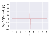
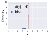
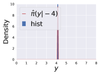
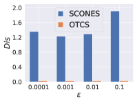
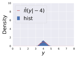
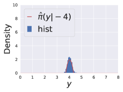
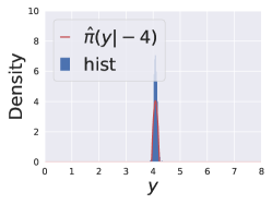
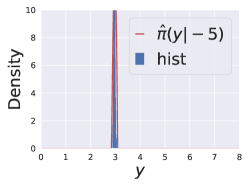
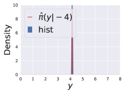
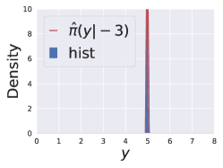
Figure 2: 1-D example of L2subscript𝐿2L_{2}-regularized unsupervised OT between p(𝐱)=𝒩(𝐱|4,1)𝑝𝐱𝒩conditional𝐱41p(\mathbf{x})=\mathcal{N}(\mathbf{x}|-4,1) and q(𝐲)=𝒩(𝐲|4,1)𝑞𝐲𝒩conditional𝐲41q(\mathbf{y})=\mathcal{N}(\mathbf{y}|4,1). (a) The gradient 𝐲logH(4,𝐲)subscript𝐲𝐻4𝐲\nabla_{\mathbf{y}}\log H(-4,\mathbf{y}). (b-c) The conditional transport plan π^(𝐲|4)^𝜋conditional𝐲4\hat{\pi}(\mathbf{y}|-4) and the histograms of generated samples by (b) SCONES and (c) OTCS with ϵ=0.0001italic-ϵ0.0001\epsilon=0.0001. (d) The distance Dis=𝔼𝐱pW2(psde(|𝐱),π(|𝐱))Dis=\mathbb{E}_{\mathbf{x}\sim p}W_{2}\left(p^{\rm sde}(\cdot|\mathbf{x}),\pi(\cdot|\mathbf{x})\right) for different ϵitalic-ϵ\epsilon computed using samples in which we approximate psde(|𝐱)p^{\rm sde}(\cdot|\mathbf{x}) and π(|𝐱)\pi(\cdot|\mathbf{x}) by Gaussian distributions with corresponding mean and variance.
Comparison with related large-scale OT methods.

Recent unsupervised OT methods [38, 39, 40, 26] often parameterize the transport map by a neural network learned by adversarial training based on the dual formulation [38, 39, 40], or generate samples from the conditional transport plan [26]. Our method is mostly related to SCONES [26] that leverages the unconditional SBDM for generating samples from the estimated conditional transport plan π^(𝐲|𝐱)^𝜋conditional𝐲𝐱\hat{\pi}(\mathbf{y}|\mathbf{x}). Motivated by the expression of π^(𝐲|𝐱)^𝜋conditional𝐲𝐱\hat{\pi}(\mathbf{y}|\mathbf{x}) in Sect. 3.5, given source sample 𝐱𝐱\mathbf{x}, SCONES generates target sample 𝐲𝐲\mathbf{y} by the reverse SDE d𝐲t=[f(𝐲t,t)g(t)2(𝐲tlogH(𝐱,𝐲t)+sθ(𝐲t;t))]dt+g(t)d𝐰¯dsubscript𝐲𝑡delimited-[]𝑓subscript𝐲𝑡𝑡𝑔superscript𝑡2subscriptsubscript𝐲𝑡𝐻𝐱subscript𝐲𝑡subscript𝑠𝜃subscript𝐲𝑡𝑡d𝑡𝑔𝑡d¯𝐰\mathop{}\!\mathrm{d}\mathbf{y}_{t}=[f(\mathbf{y}_{t},t)-g(t)^{2}\left(\nabla_{\mathbf{y}_{t}}\log H(\mathbf{x},\mathbf{y}_{t})+s_{\theta}(\mathbf{y}_{t};t)\right)]\mathop{}\!\mathrm{d}t+g(t)\mathop{}\!\mathrm{d}\bar{\mathbf{w}}, where sθ(𝐲t;t)subscript𝑠𝜃subscript𝐲𝑡𝑡s_{\theta}(\mathbf{y}_{t};t) is the unconditional score-based model. The compatibility function H𝐻H is trained on clean data. While in SCONES, 𝐲tlogH(𝐱,𝐲t)subscriptsubscript𝐲𝑡𝐻𝐱subscript𝐲𝑡\nabla_{\mathbf{y}_{t}}\log H(\mathbf{x},\mathbf{y}_{t}) is computed on noisy data 𝐲tsubscript𝐲𝑡\mathbf{y}_{t} for t>0𝑡0t>0. OTCS computes H𝐻H on clean data as in Eq. (9). We provide a 1-D example in Fig. 2 to evaluate SCONES and OTCS. From Figs. 2(b-c), we can see that the sample histogram, generated by OTCS given “-4” as condition, better fits π^(|4)\hat{\pi}(\cdot|-4). In Fig. 2(d), OTCS achieves a lower expected Wasserstein distance 𝔼𝐱pW2(psde(|𝐱),π^(|𝐱))\mathbb{E}_{\mathbf{x}\sim p}W_{2}\left(p^{\rm sde}(\cdot|\mathbf{x}),\hat{\pi}(\cdot|\mathbf{x})\right). In SCONES, the gradient of H𝐻H on noisy data could be inaccurate or zero (as shown in Fig. 2(a)), which may fail to guide the noisy data 𝐲tsubscript𝐲𝑡\mathbf{y}_{t} to move towards the desired locations as t0𝑡0t\rightarrow 0. Our OTCS utilizes H𝐻H to guide the training of the conditional score-based model, without requiring the gradient of H𝐻H in inference. This may account for the better performance of OTCS.

5 Experiments

We evaluate OTCS on unpaired super-resolution and semi-paired I2I. Due to space limits, additional experimental details and results are given in Appendix C and D, respectively.

5.1 Unpaired Super-Resolution on CelebA Faces

We consider the unpaired super-resolution for 64×\times64 aligned faces on CelebA dataset [41]. Following [26], we split the dataset into 3 disjointed subsets: A1 (90K), B1 (90K), and C1 (30K). For images in each subset, we do 2×\times bilinear downsampling to obtain the low-resolution images, followed by 2×\times bilinear upsampling to generate datasets of A0, B0, and C0 correspondingly. We train the model on A0 and B1 respectively as the source and target datasets, and test on C0 for generating high-resolution images. To apply OTCS to this task, we take B1 as target data and A0 as unpaired source data. We use the L2subscript𝐿2L_{2}-regularized unsupervised OT to estimate the coupling, where c𝑐c is set to the mean squared L2subscript𝐿2L_{2}-distance. In testing, given a degenerated image 𝐱𝐱\mathbf{x} in C0 as condition, we follow [20, 19] to sample noisy image 𝐲Msubscript𝐲𝑀\mathbf{y}_{M} from pM|0(𝐲|𝐱)subscript𝑝conditional𝑀0conditional𝐲𝐱p_{M|0}(\mathbf{y}|\mathbf{x}) as initial state and perform the reverse SDE to generate the high-resolution image. M=0.2𝑀0.2M=0.2 in experiments. Our approach is compared with recent adversarial-training-based unsupervised OT methods [42, 38, 39, 43, 40], diffusion-based unpaired I2I methods [20, 44], flow-based I2I method [45], and SCONES [26] (discussed in Sect. 4). We use the FID score [46] to measure the quality of translated images, and the SSIM metric to measure the structural similarity of each translated image to its ground-truth high-resolution image in C1.

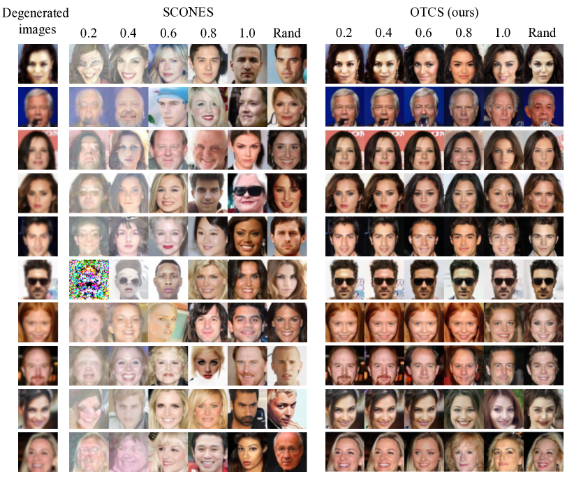
In Tab. 1, OTCS achieves the lowest FID and the highest SSIM on CelebA dataset among the compared methods. We can observe that in general, the adversarial-training-based OT methods [42, 38, 39, 40, 43] achieve better SSIM than the diffusion-based methods [20, 45, 44, 26]. This could be because the OT guidance is imposed in training by these OT methods. By contrast, the diffusion-based methods [20, 45, 44, 26] generally achieve better FID than OT methods [42, 38, 39, 40, 43], which may be attributed to the capability of diffusion models for generating high-quality images. Our OTCS imposes the OT guidance in the training of diffusion models, integrating both advantages of OT and diffusion models. In Fig. 3, we show the guided high-resolution images sampled based on OT (left) and translated images by OTCS (right). We also report the FID (0.78) and SSIM (0.9635) of the Oracle that uses true high-resolution images in A1 as paired data for training. We can see that OTCS approaches the Oracle.

Table 1: Quantitative results for unpaired super-resolution on Celeba and semi-paired I2I on Animal images and Digits. The best and second best are respectively bolded and underlined.
Method Method Type Celeba Animal images Digits
FID \downarrow SSIM \uparrow FID \downarrow Acc (%) \uparrow FID \downarrow Acc (%) \uparrow
W2GAN [42] OT 48.83 0.7169 118.45 33.56   97.06 29.13
OT-ICNN [38] OT 33.26 0.8904 148.29 38.44   50.33 10.84
OTM [39] OT 22.93 0.8302   69.27 33.11   18.67   9.48
NOT [43] OT 13.65 0.9157 156.07 28.44   23.90 15.72
KNOT [40] OT   5.95 0.8887 118.26 27.33     3.18   9.25
ReFlow [45] Flow 70.69 0.4544   56.04 29.33 138.59 11.57
EGSDE [20] Diffusion 11.49 0.3835   52.11 29.33   34.72 11.78
DDIB [44] Diffusion 11.35 0.1275   28.45 32.44     9.47   9.15
TCR [17]   34.61 40.44     6.90 36.21
SCONES [26] OT, Diffusion 15.46 0.1042   25.24 35.33     6.68 10.37
OTCS (ours) OT, Diffusion   1.77 0.9313   13.68 96.44     5.12 67.42
Refer to caption
Figure 3: Left: The guided high-resolution images (i.e., 𝐲:H(𝐱,𝐲)>0:𝐲𝐻𝐱𝐲0\mathbf{y}:H(\mathbf{x},\mathbf{y})>0) sampled based on OT for low-resolution image 𝐱𝐱\mathbf{x} in training. Right: results of OTCS on CelebA (64×\times64) in unpaired setting.

5.2 Semi-paired Image-to-Image Translation

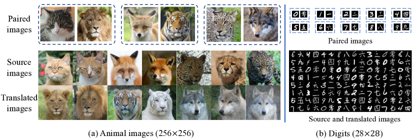
We consider the semi-paired I2I task that a large number of unpaired along with a few paired images across source and target domains are given for training. The goal of semi-paired I2I is to leverage the paired cross-domain images to guide the desired translation of source images to the target domain. To apply our approach to the semi-paired I2I, we take the source images as condition data. We use the L2subscript𝐿2L_{2}-regularized semi-supervised OT to estimate the coupling. The cost c𝑐c and csuperscript𝑐c^{\prime} in Eq. (4) are taken as the cosine dissimilarity of features using the image encoder of CLIP [47]. Apart from the compared unpaired I2I approaches in Sect. 5.1, we additionally compare our approach with the semi-paired I2I approach TCR [17]. For the OT-based approaches [42, 38, 39, 43, 40], we additionally impose the matching of the paired images using a reconstruction loss in them for semi-paired I2I. It is non-trivial to impose the matching of the paired images in the diffusion/flow-based approaches [45, 20, 44]. We adopt two metrics of FID and Accuracy (Acc). The FID measures the quality of generated samples. The higher Acc implies that the guidance of the paired images is better realized for desired translation. The experiments are conducted on digits and natural animal images.
Refer to caption
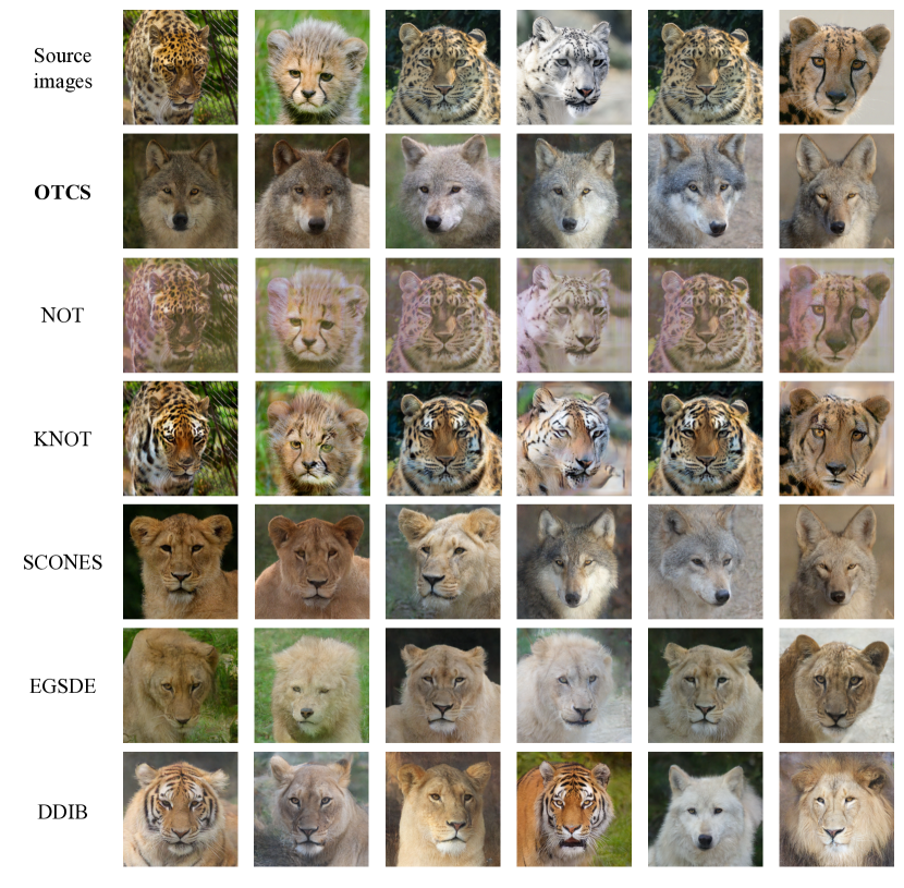
Figure 4: Results of OTCS for semi-paired I2I on (a) Animal images and (b) Digits. The bottom of Fig. 4(b) plots source (odd columns) and corresponding translated (even columns) images.
Refer to caption
Refer to caption
Refer to caption
Refer to caption
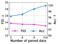
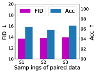
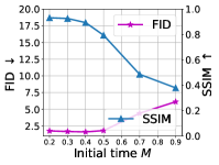
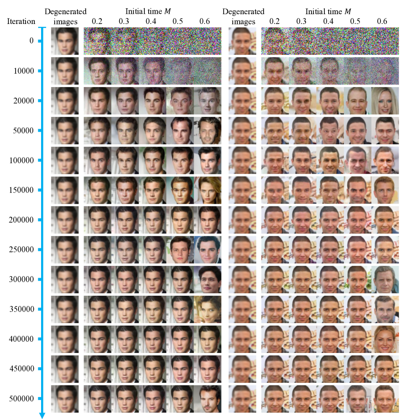
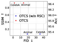
Figure 5: (a) Results of OTCS w/ and w/o RSC. (b-c) Results of OTCS with varying (b) numbers and (c) samplings of paired data on Animal images. (d) Results of OTCS for different M𝑀M on CelebA.

For Animal images, we take images of cat, fox, and leopard from AFHQ [48] dataset as source, and images of lion, tiger, and wolf as target. Three cross-domain image pairs are given, as shown in Fig. 4(a). By the guidance of the paired images, we expect that the cat, fox, and leopard images are respectively translated to the images of lion, tiger, and wolf. The Acc is the ratio of source images translated to ground-truth translated classes (GTTCs), where the GTTCs of source images of cat/fox/leopard are lion/tiger/wolf. For Digits, we consider the translation from MNIST [49] to Chinese-MNIST [50]. The MNIST and Chinese-MNIST contain the digits (from 0 to 9) in different modalities. We annotate 10 cross-domain image pairs, each corresponding to a digit, as in Fig. 4(b). With the guidance of the paired images, we expect that the source images are translated to the target ones representing the same digits. The GTTCs for the source images are their corresponding digits.

We can observe in Tab. 1 that OTCS achieves the highest Acc on both Animal images and Digits, outperforming the second-best method TCR [17] by more than 50% and 30% on the two datasets, respectively. Our approach explicitly models the guidance of the paired images to the unpaired ones using the semi-supervised OT in training, and better translates the source images to target ones of the desired classes. In terms of the FID, OTCS achieves competitive (on Digits) or even superior (on Animal images) results over the other approaches, indicating that OTCS can generate images of comparable quality. The translated images in Figs. 4 also show the effectiveness of OTCS.

5.3 Analysis

Effectiveness of resampling-by-compatibility (RSC). Figure 5 shows that OTCS achieves better results (left top points are better) than OTCS (w/o RSC) in semi-paired I2I on Animal images and unpaired super-resolution on CelebA, demonstrating the effectiveness of resampling-by-compatibility.

Results on semi-paired I2I with varying numbers and samplings of paired images. We study the effect of the number and choice of paired images in semi-paired I2I. Figure 5 shows that as the number of paired data increases, the Acc increases, and the FID marginally decreases. This implies that our approach can impose the guidance of different amounts of paired data to translate source images to desired classes. From Fig. 5, OTCS achieves similar FID and Acc for three different samplings of the same number, i.e., 3, of paired images (denoted as “S1”, “S2”, and “S3” in Fig. 5).

Results on unpaired super-resolution with varying initial time. We show the results of OTCS under different initial time M𝑀M in the reverse SDE. Figure 5 indicates that with a smaller M𝑀M, our OTCS achieves better SSIM. This makes sense because adding smaller-scale noise in inference could better preserve the structure of source data in SBDMs, as in [19, 20]. However, smaller M𝑀M may lead to a larger distribution gap/FID between generated and target data for SBDMs with unconditional score-based model [19, 20]. We observe that OTCS achieves the FID below 1.85 for M𝑀M in [0.2, 0.5].

6 Conclusion

This paper proposes a novel Optimal Transport-guided Conditional Score-based diffusion model (OTCS) for image translation with unpaired or partially paired training dataset. We build the coupling of the condition data and target data using L2subscript𝐿2L_{2}-regularized unsupervised and semi-supervised OTs, and present the OT-guided conditional denoising score-matching and resampling-by-compatibility to train the conditional score-based model. Extensive experiments in unpaired super-resolution and semi-paired I2I tasks demonstrated the effectiveness of OTCS for achieving desired translation of source images. We theoretically analyze that OTCS realizes data transport for OT. In the future, we are interested in more applications of OTCS, such as medical image translation/synthesis.

Limitations

The cost function should be determined first when using our method. In experiments, we simply choose the squared L2subscript𝐿2L_{2}-distance in image space for unpaired super-resolution and cosine distance in feature space for semi-paired I2I, achieving satisfactory performance. However, the performance may be improved if more domain knowledge is employed to define the cost function. Meanwhile, if the number of target data is small, the generation ability of our trained model may be limited.

Acknowledgement

This work was supported by National Key R&D Program 2021YFA1003002 and NSFC (12125104, U20B2075, 61721002).

References

  • [1] Yang Song and Stefano Ermon. Generative modeling by estimating gradients of the data distribution. In NeurIPS, 2019.
  • [2] Jonathan Ho, Ajay Jain, and Pieter Abbeel. Denoising diffusion probabilistic models. In NeurIPS, 2020.
  • [3] Yang Song, Jascha Sohl-Dickstein, Diederik P Kingma, Abhishek Kumar, Stefano Ermon, and Ben Poole. Score-based generative modeling through stochastic differential equations. In ICLR, 2021.
  • [4] Alexander Quinn Nichol and Prafulla Dhariwal. Improved denoising diffusion probabilistic models. In ICML, 2021.
  • [5] Fan Bao, Chongxuan Li, Jun Zhu, and Bo Zhang. Analytic-DPM: an analytic estimate of the optimal reverse variance in diffusion probabilistic models. In ICLR, 2022.
  • [6] Prafulla Dhariwal and Alexander Nichol. Diffusion models beat gans on image synthesis. In M. Ranzato, A. Beygelzimer, Y. Dauphin, P.S. Liang, and J. Wortman Vaughan, editors, NeurIPS, 2021.
  • [7] Tero Karras, Miika Aittala, Timo Aila, and Samuli Laine. Elucidating the design space of diffusion-based generative models. In NeurIPS, 2022.
  • [8] Zixiang Zhao, Haowen Bai, Yuanzhi Zhu, Jiangshe Zhang, Shuang Xu, Yulun Zhang, Kai Zhang, Deyu Meng, Radu Timofte, and Luc Van Gool. Ddfm: Denoising diffusion model for multi-modality image fusion. In ICCV, 2023.
  • [9] Prafulla Dhariwal and Alexander Nichol. Diffusion models beat gans on image synthesis. In NeurIPS, 2021.
  • [10] Chitwan Saharia, Jonathan Ho, William Chan, Tim Salimans, David J Fleet, and Mohammad Norouzi. Image super-resolution via iterative refinement. IEEE Trans. PAMI, In press, 2022.
  • [11] Jay Whang, Mauricio Delbracio, Hossein Talebi, Chitwan Saharia, Alexandros G Dimakis, and Peyman Milanfar. Deblurring via stochastic refinement. In CVPR, 2022.
  • [12] Chitwan Saharia, William Chan, Saurabh Saxena, Lala Li, Jay Whang, Emily Denton, Seyed Kamyar Seyed Ghasemipour, Burcu Karagol Ayan, S Sara Mahdavi, Rapha Gontijo Lopes, et al. Photorealistic text-to-image diffusion models with deep language understanding. In NeurIPS, 2022.
  • [13] Jonathan Ho and Tim Salimans. Classifier-free diffusion guidance. In NeurIPS 2021 Workshop on Deep Generative Models and Downstream Applications, 2021.
  • [14] Zixiang Zhao, Jiangshe Zhang, Shuang Xu, Zudi Lin, and Hanspeter Pfister. Discrete cosine transform network for guided depth map super-resolution. In CVPR, 2022.
  • [15] Zixiang Zhao, Jiangshe Zhang, Xiang Gu, Chengli Tan, Shuang Xu, Yulun Zhang, Radu Timofte, and Luc Van Gool. Spherical space feature decomposition for guided depth map super-resolution. In ICCV, 2023.
  • [16] Jun-Yan Zhu, Taesung Park, Phillip Isola, and Alexei A Efros. Unpaired image-to-image translation using cycle-consistent adversarial networks. In ICCV, 2017.
  • [17] Aamir Mustafa and Rafał K Mantiuk. Transformation consistency regularization–a semi-supervised paradigm for image-to-image translation. In ECCV, 2020.
  • [18] Jooyoung Choi, Sungwon Kim, Yonghyun Jeong, Youngjune Gwon, and Sungroh Yoon. Ilvr: Conditioning method for denoising diffusion probabilistic models. In ICCV, 2021.
  • [19] Chenlin Meng, Yutong He, Yang Song, Jiaming Song, Jiajun Wu, Jun-Yan Zhu, and Stefano Ermon. Sdedit: Guided image synthesis and editing with stochastic differential equations. In ICLR, 2022.
  • [20] Min Zhao, Fan Bao, Chongxuan Li, and Jun Zhu. Egsde: Unpaired image-to-image translation via energy-guided stochastic differential equations. In NurIPS, 2022.
  • [21] Xuan Su, Jiaming Song, Chenlin Meng, and Stefano Ermon. Dual diffusion implicit bridges for image-to-image translation. In ICLR, 2023.
  • [22] Xi Yu, Xiang Gu, Haozhi Liu, and Jian Sun. Constructing non-isotropic gaussian diffusion model using isotropic gaussian diffusion model. In NeurIPS, 2023.
  • [23] Valentin Khrulkov, Gleb Ryzhakov, Andrei Chertkov, and Ivan Oseledets. Understanding DDPM latent codes through optimal transport. In ICLR, 2023.
  • [24] Zezeng Li, ShengHao Li, Zhanpeng Wang, Na Lei, Zhongxuan Luo, and Xianfeng Gu. Dpm-ot: A new diffusion probabilistic model based on optimal transport. In ICCV, 2023.
  • [25] Valentin De Bortoli, James Thornton, Jeremy Heng, and Arnaud Doucet. Diffusion schrödinger bridge with applications to score-based generative modeling. In NeurIPS, 2021.
  • [26] Max Daniels, Tyler Maunu, and Paul Hand. Score-based generative neural networks for large-scale optimal transport. In NeurIPS, 2021.
  • [27] Cédric Villani. Optimal transport: old and new, volume 338. Springer, 2009.
  • [28] Xiang Gu, Yucheng Yang, Wei Zeng, Jian Sun, and Zongben Xu. Keypoint-guided optimal transport with applications in heterogeneous domain adaptation. In NeurIPS, 2022.
  • [29] Leonid V Kantorovich. On the translocation of masses. In Dokl. Akad. Nauk. USSR (NS), 1942.
  • [30] Xiang Gu, Liwei Yang, Jian Sun, and Zongben Xu. Optimal transport-guided conditional score-based diffusion model. In NeurIPS, 2023.
  • [31] Vivien Seguy, Bharath Bhushan Damodaran, Rémi Flamary, Nicolas Courty, Antoine Rolet, and Mathieu Blondel. Large-scale optimal transport and mapping estimation. In ICLR, 2018.
  • [32] Xiang Gu, Yucheng Yang, Wei Zeng, Jian Sun, and Zongben Xu. Keypoint-guided optimal transport. arXiv preprint arXiv:2303.13102, 2023.
  • [33] Eckhard Platen. An introduction to numerical methods for stochastic differential equations. Acta Numer., 8:197–246, 1999.
  • [34] Jiaming Song, Chenlin Meng, and Stefano Ermon. Denoising diffusion implicit models. In ICLR, 2021.
  • [35] Cheng Lu, Yuhao Zhou, Fan Bao, Jianfei Chen, Chongxuan Li, and Jun Zhu. DPM-solver: A fast ODE solver for diffusion probabilistic model sampling in around 10 steps. In NeurIPS, 2022.
  • [36] Aude Genevay, Marco Cuturi, Gabriel Peyré, and Francis Bach. Stochastic optimization for large-scale optimal transport. In NeurIPS, 2016.
  • [37] Dohyun Kwon, Ying Fan, and Kangwook Lee. Score-based generative modeling secretly minimizes the wasserstein distance. In NeurIPS, 2022.
  • [38] Ashok Makkuva, Amirhossein Taghvaei, Sewoong Oh, and Jason Lee. Optimal transport mapping via input convex neural networks. In ICML, 2020.
  • [39] Litu Rout, Alexander Korotin, and Evgeny Burnaev. Generative modeling with optimal transport maps. In ICLR, 2022.
  • [40] Alexander Korotin, Daniil Selikhanovych, and Evgeny Burnaev. Kernel neural optimal transport. In ICLR, 2023.
  • [41] Ziwei Liu, Ping Luo, Xiaogang Wang, and Xiaoou Tang. Deep learning face attributes in the wild. In ICCV, 2015.
  • [42] Leygonie Jacob, Jennifer She, Amjad Almahairi, Sai Rajeswar, and Aaron Courville. W2gan: Recovering an optimal transport map with a gan. In ICLR, 2019.
  • [43] Alexander Korotin, Daniil Selikhanovych, and Evgeny Burnaev. Neural optimal transport. In ICLR, 2023.
  • [44] Xuan Su, Jiaming Song, Chenlin Meng, and Stefano Ermon. Dual diffusion implicit bridges for image-to-image translation. In ICLR, 2023.
  • [45] Xingchao Liu, Chengyue Gong, and qiang liu. Flow straight and fast: Learning to generate and transfer data with rectified flow. In ICLR, 2023.
  • [46] Martin Heusel, Hubert Ramsauer, Thomas Unterthiner, Bernhard Nessler, and Sepp Hochreiter. Gans trained by a two time-scale update rule converge to a local nash equilibrium. In NeurIPS, 2017.
  • [47] Alec Radford, Jong Wook Kim, Chris Hallacy, Aditya Ramesh, Gabriel Goh, Sandhini Agarwal, Girish Sastry, Amanda Askell, Pamela Mishkin, Jack Clark, et al. Learning transferable visual models from natural language supervision. In ICML, 2021.
  • [48] Yunjey Choi, Youngjung Uh, Jaejun Yoo, and Jung-Woo Ha. Stargan v2: Diverse image synthesis for multiple domains. In CVPR, 2020.
  • [49] Yann LeCun, Léon Bottou, Yoshua Bengio, and Patrick Haffner. Gradient-based learning applied to document recognition. Proceedings of the IEEE, 86(11):2278–2324, 1998.
  • [50] https://www.kaggle.com/datasets/gpreda/chinese-mnist.
  • [51] Diederik P Kingma and Max Welling. Auto-encoding variational bayes. In ICLR, 2014.
  • [52] Pascal Vincent. A connection between score matching and denoising autoencoders. Neural computation, 23(7):1661–1674, 2011.
  • [53] Gabriel Peyré, Marco Cuturi, et al. Computational optimal transport: With applications to data science. Foundations and Trends® in Machine Learning, 11(5-6):355–607, 2019.
  • [54] Adam Paszke, Sam Gross, Francisco Massa, Adam Lerer, James Bradbury, Gregory Chanan, Trevor Killeen, Zeming Lin, Natalia Gimelshein, Luca Antiga, et al. Pytorch: An imperative style, high-performance deep learning library. In NeurIPS, 2019.

Appendix

Appendix A Additional Details for Sections 2 and 3

A.1 Additional Details for Section 2

Details of VP-SDE and VE-SDE.

As mentioned in Sect. 2.1, we choose the VE-SDE and the VP-SDE as the forward SDEs. For VE-SDE, f(𝐲,t)=0𝑓𝐲𝑡0f(\mathbf{y},t)=0 and g(t)=αt𝑔𝑡superscript𝛼𝑡g(t)=\alpha^{t} where α𝛼\alpha is a hyper-parameter. For VP-SDE, f(𝐲,t)=12β(t)𝐲𝑓𝐲𝑡12𝛽𝑡𝐲f(\mathbf{y},t)=-\frac{1}{2}\beta(t)\mathbf{y} and g(t)=β(t)𝑔𝑡𝛽𝑡g(t)=\sqrt{\beta(t)} where β(t)=βmin+(βmaxβmin)t𝛽𝑡subscript𝛽minsubscript𝛽maxsubscript𝛽min𝑡\beta(t)=\beta_{\rm min}+(\beta_{\rm max}-\beta_{\rm min})t, and βminsubscript𝛽min\beta_{\rm min} and βmaxsubscript𝛽max\beta_{\rm max} are hyper-parameters. Then, the conditional distribution, a.k.a., permutation kernel, pt|0(𝐲t|𝐲0)subscript𝑝conditional𝑡0conditionalsubscript𝐲𝑡subscript𝐲0p_{t|0}(\mathbf{y}_{t}|\mathbf{y}_{0}) of 𝐲tsubscript𝐲𝑡\mathbf{y}_{t} given 𝐲0subscript𝐲0\mathbf{y}_{0} is

pt|0(𝐲t|𝐲0)={𝒩(𝐲t|𝐲0,12logα(α2t1)𝐈)), for VE-SDE, 𝒩(𝐲t|𝐲0e12h(t),(1eh(t))𝐈), for VP-SDE, p_{t|0}(\mathbf{y}_{t}|\mathbf{y}_{0})=\begin{cases}\mathcal{N}\left(\mathbf{y}_{t}|{\bf\mathbf{y}}_{0},\frac{1}{2\log\alpha}(\alpha^{2t}-1)\bf{I})\right),&\mbox{ for VE-SDE, }\\ \mathcal{N}\left(\mathbf{y}_{t}|\mathbf{y}_{0}e^{\frac{1}{2}h(t)},(1-e^{h(t)}){\bf I}\right),&\mbox{ for VP-SDE, }\end{cases} (A-1)

where h(t)=12t2(βmaxβmin)tβmin𝑡12superscript𝑡2subscript𝛽maxsubscript𝛽min𝑡subscript𝛽minh(t)=-\frac{1}{2}t^{2}(\beta_{\rm max}-\beta_{\rm min})-t\beta_{\rm min}, and 𝐈𝐈\bf I is the identity matrix. Following [3], we set T𝑇T to 111, and pprior=𝒩(0,𝐈)subscript𝑝prior𝒩0𝐈p_{\rm prior}=\mathcal{N}(0,\mathbf{I}) for VP-SDE and pprior=𝒩(0,12logα(α2t1)𝐈)subscript𝑝prior𝒩012𝛼superscript𝛼2𝑡1𝐈p_{\rm prior}=\mathcal{N}(0,\frac{1}{2\log\alpha}(\alpha^{2t}-1)\mathbf{I}) for VE-SDE.

Pseudo-codes of algorithm for training uω,vωsubscript𝑢𝜔subscript𝑣𝜔{u_{\omega},v_{\omega}}.

The pseudo-codes of the algorithm to learn the dual variables uω,vωsubscript𝑢𝜔subscript𝑣𝜔u_{\omega},v_{\omega}, a.k.a., potentials, are given in Algorithm 1.

Input: Distribution p𝑝p of conditions, target data distribution q𝑞q, paired data (if available)
Output: Learned potentials uω^,vω^subscript𝑢^𝜔subscript𝑣^𝜔u_{\hat{\omega}},v_{\hat{\omega}}
for iter=1,,Niteriter1superscriptsubscript𝑁iter{\rm iter}=1,\cdots,N_{\rm iter}^{\prime} do
       Sampling mini-batch data 𝑿={𝐱b}b=1B𝑿superscriptsubscriptsubscript𝐱𝑏𝑏1superscript𝐵\bm{X}=\{\mathbf{x}_{b}\}_{b=1}^{B^{\prime}} from p𝑝p, 𝒀={𝐲b}b=1B𝒀superscriptsubscriptsubscript𝐲𝑏𝑏1superscript𝐵\bm{Y}=\{\mathbf{y}_{b}\}_{b=1}^{B^{\prime}} from q𝑞q;
       if paired data are available then
            Computing the loss of semi-supervised OT in Eq. (6) on 𝑿𝑿\bm{X} and 𝒀𝒀\bm{Y};
      else
            Computing the loss of unsupervised OT in Eq. (6) on 𝑿𝑿\bm{X} and 𝒀𝒀\bm{Y};
       end if
      Backward propagation to compute the gradient and update ω𝜔\omega using Adam algorithm;
      
end for
ω^=ω^𝜔𝜔\hat{\omega}=\omega.
Algorithm 1 Algorithm for estimating potentials uω^,vω^subscript𝑢^𝜔subscript𝑣^𝜔u_{\hat{\omega}},v_{\hat{\omega}}

A.2 Additional Details for Section 3

Rationality of the resampling-by-compatibility.

We next explain the rationality of the resampling-by-compatibility presented in Sect. 3.3. For the convenience of description, for any 𝐱,𝐲𝐱𝐲\mathbf{x},\mathbf{y}, we denote

𝒥𝐱,𝐲=𝔼twt𝔼𝐲tpt|0(𝐲t|𝐲)sθ(𝐲t;𝐱,t)𝐲tlogpt|0(𝐲t|𝐲)22.\mathcal{J}_{\mathbf{x},\mathbf{y}}=\mathbb{E}_{t}w_{t}\mathbb{E}_{\mathbf{y}_{t}\sim p_{t|0}(\mathbf{y}_{t}|\mathbf{y})}\|s_{\theta}(\mathbf{y}_{t};\mathbf{x},t)-\nabla_{\mathbf{y}_{t}}\log p_{t|0}(\mathbf{y}_{t}|\mathbf{y})\|_{2}^{2}. (A-2)

The training loss 𝒥CDSM(θ)subscript𝒥CDSM𝜃\mathcal{J}_{\rm CDSM}(\theta) in Eq. (9) can be written as

𝒥CDSM(θ)=𝔼𝐱p𝔼𝐲qH(𝐱,𝐲)𝒥𝐱,𝐲.subscript𝒥CDSM𝜃subscript𝔼similar-to𝐱𝑝subscript𝔼similar-to𝐲𝑞𝐻𝐱𝐲subscript𝒥𝐱𝐲\mathcal{J}_{\rm CDSM}(\theta)={\mathbb{E}}_{\mathbf{x}\sim p}{\mathbb{E}}_{\mathbf{y}\sim q}H(\mathbf{x},\mathbf{y})\mathcal{J}_{\mathbf{x},\mathbf{y}}. (A-3)

By the resampling-by-compatibility, q𝑞q is approximated based on samples 𝐘𝐱subscript𝐘𝐱\mathbf{Y}_{\mathbf{x}} by q(𝐲)1Ll=1Lδ(𝐲𝐲l)𝑞𝐲1𝐿superscriptsubscript𝑙1𝐿𝛿𝐲superscript𝐲𝑙q(\mathbf{y})\approx\frac{1}{L}\sum_{l=1}^{L}\delta(\mathbf{y}-\mathbf{y}^{l}). We then have

𝒥CDSM(θ)𝔼𝐱p1Ll=1LH(𝐱,𝐲l)𝒥𝐱,𝐲l𝔼𝐱p1H0l=1LH(𝐱,𝐲l)𝒥𝐱,𝐲l=𝔼𝐱p𝔼𝐲h~𝐱𝒥𝐱,𝐲,subscript𝒥CDSM𝜃subscript𝔼similar-to𝐱𝑝1𝐿superscriptsubscript𝑙1𝐿𝐻𝐱superscript𝐲𝑙subscript𝒥𝐱superscript𝐲𝑙proportional-tosubscript𝔼similar-to𝐱𝑝1subscript𝐻0superscriptsubscript𝑙1𝐿𝐻𝐱superscript𝐲𝑙subscript𝒥𝐱superscript𝐲𝑙subscript𝔼similar-to𝐱𝑝subscript𝔼similar-to𝐲subscript~𝐱subscript𝒥𝐱𝐲\begin{split}\mathcal{J}_{\rm CDSM}(\theta)&\approx{\mathbb{E}}_{\mathbf{x}\sim p}\frac{1}{L}\sum_{l=1}^{L}H(\mathbf{x},\mathbf{y}^{l})\mathcal{J}_{\mathbf{x},\mathbf{y}^{l}}\\ &\propto{\mathbb{E}}_{\mathbf{x}\sim p}\frac{1}{H_{0}}\sum_{l=1}^{L}H(\mathbf{x},\mathbf{y}^{l})\mathcal{J}_{\mathbf{x},\mathbf{y}^{l}}\\ &={\mathbb{E}}_{\mathbf{x}\sim p}\mathbb{E}_{\mathbf{y}\sim\tilde{h}_{\mathbf{x}}}\mathcal{J}_{\mathbf{x},\mathbf{y}},\end{split} (A-4)

where H0=l=1LH(𝐱,𝐲l)subscript𝐻0superscriptsubscript𝑙1𝐿𝐻𝐱superscript𝐲𝑙H_{0}=\sum_{l=1}^{L}H(\mathbf{x},\mathbf{y}^{l}) and h~𝐱subscript~𝐱\tilde{h}_{\mathbf{x}} is the distribution defined on 𝒀𝐱subscript𝒀𝐱\bm{Y}_{\mathbf{x}} as h~𝐱(𝐲)=1H0l=1LH(𝐱,𝐲l)δ(𝐲𝐲l)subscript~𝐱𝐲1subscript𝐻0superscriptsubscript𝑙1𝐿𝐻𝐱superscript𝐲𝑙𝛿𝐲superscript𝐲𝑙\tilde{h}_{\mathbf{x}}(\mathbf{y})=\frac{1}{H_{0}}\sum_{l=1}^{L}H(\mathbf{x},\mathbf{y}^{l})\delta(\mathbf{y}-\mathbf{y}^{l}). Equation (A-4) indicates that 𝒥CDSM(θ)subscript𝒥CDSM𝜃\mathcal{J}_{\rm CDSM}(\theta) can be approximately implemented based on samples using our resampling-by-compatibility strategy. More concretely, the last line in Eq. (A-4) can be implemented by sequentially dropping 𝐱𝐱\mathbf{x} from p𝑝p, generating samples 𝒀𝐱subscript𝒀𝐱\bm{Y}_{\mathbf{x}} to construct h~𝐱subscript~𝐱\tilde{h}_{\mathbf{x}}, sampling 𝐲𝐲\mathbf{y} from h~𝐱subscript~𝐱\tilde{h}_{\mathbf{x}}, and computing 𝒥𝐱,𝐲subscript𝒥𝐱𝐲\mathcal{J}_{\mathbf{x},\mathbf{y}} on (𝐱,𝐲)𝐱𝐲(\mathbf{x},\mathbf{y}). Note that dropping sample 𝐲𝐲\mathbf{y} from h~𝐱subscript~𝐱\tilde{h}_{\mathbf{x}} means to choose a 𝐲𝐲\mathbf{y} from 𝒀𝐱subscript𝒀𝐱\bm{Y}_{\mathbf{x}} with the probability proportional to H(𝐱,𝐲l)𝐻𝐱superscript𝐲𝑙H(\mathbf{x},\mathbf{y}^{l}).

Training by fitting noise.

Based on Eq. (A-1), pt|0(𝐲t|𝐲)subscript𝑝conditional𝑡0conditionalsubscript𝐲𝑡𝐲p_{t|0}(\mathbf{y}_{t}|\mathbf{y}) is a Gaussian distribution. We denote the σt𝐈subscript𝜎𝑡𝐈\sigma_{t}\mathbf{I} as the standard variation of pt|0(𝐲t|𝐲)subscript𝑝conditional𝑡0conditionalsubscript𝐲𝑡𝐲p_{t|0}(\mathbf{y}_{t}|\mathbf{y}), i.e., σt2=12logα(α2t1)superscriptsubscript𝜎𝑡212𝛼superscript𝛼2𝑡1\sigma_{t}^{2}=\frac{1}{2\log\alpha}(\alpha^{2t}-1) for VE-SDE, and σt2=1eh(t)superscriptsubscript𝜎𝑡21superscript𝑒𝑡\sigma_{t}^{2}=1-e^{h(t)} for VP-SDE. Using the reparameterization trick [51], given 𝐱,𝐲𝐱𝐲\mathbf{x},\mathbf{y} sampled using our resampling-by-compatibility, we have 𝐲t=𝐲+σtϵsubscript𝐲𝑡𝐲subscript𝜎𝑡bold-italic-ϵ\mathbf{y}_{t}=\mathbf{y}+\sigma_{t}\bm{\epsilon} for VE-SDE, and 𝐲t=e12h(t)𝐲+σtϵsubscript𝐲𝑡superscript𝑒12𝑡𝐲subscript𝜎𝑡bold-italic-ϵ\mathbf{y}_{t}=e^{\frac{1}{2}h(t)}\mathbf{y}+\sigma_{t}\bm{\epsilon} for VP-SDE, where ϵ𝒩(0,𝐈)similar-tobold-italic-ϵ𝒩0𝐈\bm{\epsilon}\sim\mathcal{N}(0,\mathbf{I}). Further, 𝐲tlogpt|0(𝐲t|𝐲)=1σtϵsubscriptsubscript𝐲𝑡subscript𝑝conditional𝑡0conditionalsubscript𝐲𝑡𝐲1subscript𝜎𝑡bold-italic-ϵ\nabla_{\mathbf{y}_{t}}\log p_{t|0}(\mathbf{y}_{t}|\mathbf{y})=-\frac{1}{\sigma_{t}}\bm{\epsilon}. Therefore, the loss 𝒥𝐱,𝐲subscript𝒥𝐱𝐲\mathcal{J}_{\mathbf{x},\mathbf{y}} in Eq. (A-2) can be written as

𝒥𝐱,𝐲=𝔼t,ϵ𝒩(0,𝐈)[wtσt2sθ(𝒖t(𝐲)+σtϵ;𝐱,t)σt+ϵ22].subscript𝒥𝐱𝐲subscript𝔼similar-to𝑡bold-italic-ϵ𝒩0𝐈delimited-[]subscript𝑤𝑡superscriptsubscript𝜎𝑡2superscriptsubscriptnormsubscript𝑠𝜃subscript𝒖𝑡𝐲subscript𝜎𝑡bold-italic-ϵ𝐱𝑡subscript𝜎𝑡bold-italic-ϵ22\mathcal{J}_{\mathbf{x},\mathbf{y}}={\mathbb{E}}_{t,\bm{\epsilon}\sim\mathcal{N}(0,\mathbf{I})}\left[\frac{w_{t}}{\sigma_{t}^{2}}\left\|s_{\theta}(\bm{u}_{t}(\mathbf{y})+\sigma_{t}\bm{\epsilon};\mathbf{x},t)\sigma_{t}+\bm{\epsilon}\right\|_{2}^{2}\right]. (A-5)

where 𝒖t(𝐲)=𝐲subscript𝒖𝑡𝐲𝐲\bm{u}_{t}(\mathbf{y})=\mathbf{y} for VE-SDE, and 𝒖t(𝐲)=e12h(t)𝐲subscript𝒖𝑡𝐲superscript𝑒12𝑡𝐲\bm{u}_{t}(\mathbf{y})=e^{\frac{1}{2}h(t)}\mathbf{y} for VP-SDE. Equation (A-5) implies that sθ(𝐲t;𝐱,t)subscript𝑠𝜃subscript𝐲𝑡𝐱𝑡s_{\theta}(\mathbf{y}_{t};\mathbf{x},t) is trained to fit the scaled noise 1σtϵ1subscript𝜎𝑡bold-italic-ϵ-\frac{1}{\sigma_{t}}\bm{\epsilon}.

Pseudo-codes of algorithm training sθsubscript𝑠𝜃{s_{\theta}}.

The pseudo-codes of the algorithm to train sθsubscript𝑠𝜃s_{\theta} for the case where training data consist of condition dataset 𝒟𝐱subscript𝒟𝐱\mathcal{D}_{\mathbf{x}} and target dataset 𝒟𝐲subscript𝒟𝐲\mathcal{D}_{\mathbf{y}} are given in Algorithm 2. The pseudo-codes of the algorithm to train sθsubscript𝑠𝜃s_{\theta} for the case with continuous distributions p,q𝑝𝑞p,q are given in Algorithm 3.

Input: Condition dataset 𝒟𝐱subscript𝒟𝐱\mathcal{D}_{\mathbf{x}}, target dataset 𝒟𝐲subscript𝒟𝐲\mathcal{D}_{\mathbf{y}}, paired data (if available)
Output: Trained conditional score-based model sθ^subscript𝑠^𝜃s_{\hat{\theta}}
Learning potentials uω^,vω^subscript𝑢^𝜔subscript𝑣^𝜔u_{\hat{\omega}},v_{\hat{\omega}} using Algorithm 1;
// Computing and storing H𝐻H for target samples with non-zero H𝐻H
Dict={}𝐷𝑖𝑐𝑡Dict=\{\};
for 𝐱𝐱\mathbf{x} in 𝒟𝐱subscript𝒟𝐱\mathcal{D}_{\mathbf{x}} do
       𝒀𝐱={𝐲:H(𝐱,𝐲)>0,𝐲𝒟𝐲}subscript𝒀𝐱conditional-set𝐲formulae-sequence𝐻𝐱𝐲0𝐲subscript𝒟𝐲\bm{Y}_{\mathbf{x}}=\{\mathbf{y}:H(\mathbf{x},\mathbf{y})>0,\mathbf{y}\in\mathcal{D}_{\mathbf{y}}\};
       𝑯𝐱={H(𝐱,𝐲)H0:𝐲𝒀𝐱}subscript𝑯𝐱conditional-set𝐻𝐱𝐲subscript𝐻0𝐲subscript𝒀𝐱\bm{H}_{\mathbf{x}}=\{\frac{H(\mathbf{x},\mathbf{y})}{H_{0}}:\mathbf{y}\in\bm{Y}_{\mathbf{x}}\}, where H0=𝐲𝒀𝐱H(𝐱,𝐲)subscript𝐻0subscript𝐲subscript𝒀𝐱𝐻𝐱𝐲H_{0}=\sum_{\mathbf{y}\in\bm{Y}_{\mathbf{x}}}H(\mathbf{x},\mathbf{y});
       Dict=Dict{(𝒀𝐱,𝑯𝐱)}𝐷𝑖𝑐𝑡𝐷𝑖𝑐𝑡subscript𝒀𝐱subscript𝑯𝐱Dict=Dict\cup\{(\bm{Y}_{\mathbf{x}},\bm{H}_{\mathbf{x}})\};
      
end for
// Traning sθsubscript𝑠𝜃s_{\theta} on mini-batch data
for iter=1,,Niteriter1subscript𝑁iter{\rm iter}=1,\cdots,N_{\rm iter} do
       Sampling mini-batch data {𝐱b}b=1Bsuperscriptsubscriptsubscript𝐱𝑏𝑏1𝐵\{\mathbf{x}_{b}\}_{b=1}^{B} from 𝒟𝐱subscript𝒟𝐱\mathcal{D}_{\mathbf{x}};
       for b=1,2,,B𝑏12𝐵b=1,2,\cdots,B do
            // Resampling-by-compatibility
             Finding (𝒀𝐱b,𝑯𝐱b)subscript𝒀subscript𝐱𝑏subscript𝑯subscript𝐱𝑏(\bm{Y}_{\mathbf{x}_{b}},\bm{H}_{{\mathbf{x}}_{b}}) in Dict𝐷𝑖𝑐𝑡Dict ;
             Choosing 𝐲bsubscript𝐲𝑏\mathbf{y}_{b} from 𝒀𝐱bsubscript𝒀subscript𝐱𝑏\bm{Y}_{\mathbf{x}_{b}} with probability 𝑯𝐱bsubscript𝑯subscript𝐱𝑏\bm{H}_{{\mathbf{x}}_{b}};
             Sampling tbsubscript𝑡𝑏t_{b} from 𝒰([0,T])𝒰0𝑇\mathcal{U}([0,T]), and ϵbsubscriptbold-italic-ϵ𝑏\bm{\epsilon}_{b} from 𝒩(0,𝐈)𝒩0𝐈\mathcal{N}(0,\mathbf{I});
            
       end for
      Computing loss 1Bb=1Bwtbσtb2sθ(𝒖tb(𝐲b)+σtbϵb;𝐱b,tb)σtb+ϵb221𝐵superscriptsubscript𝑏1𝐵subscript𝑤subscript𝑡𝑏superscriptsubscript𝜎subscript𝑡𝑏2superscriptsubscriptnormsubscript𝑠𝜃subscript𝒖subscript𝑡𝑏subscript𝐲𝑏subscript𝜎subscript𝑡𝑏subscriptbold-italic-ϵ𝑏subscript𝐱𝑏subscript𝑡𝑏subscript𝜎subscript𝑡𝑏subscriptbold-italic-ϵ𝑏22\frac{1}{B}\sum_{b=1}^{B}\frac{w_{t_{b}}}{\sigma_{t_{b}}^{2}}\left\|s_{\theta}\left(\bm{u}_{t_{b}}(\mathbf{y}_{b})+\sigma_{t_{b}}\bm{\epsilon}_{b};\mathbf{x}_{b},t_{b}\right)\sigma_{t_{b}}+\bm{\epsilon}_{b}\right\|_{2}^{2} ;
        // Eq. (A-5)
       Backward propagation to compute the gradient w.r.t. θ𝜃\theta and update θ𝜃\theta using Adam algorithm;
      
end for
θ^=θ^𝜃𝜃\hat{\theta}=\theta.
Algorithm 2 Training algorithm for discrete datasets
Input: Condition distribution p𝑝p, data distribution q𝑞q, paired data (if available)
Output: Trained conditional score-based model sθ^subscript𝑠^𝜃s_{\hat{\theta}}
Learning potentials uω^,vω^subscript𝑢^𝜔subscript𝑣^𝜔u_{\hat{\omega}},v_{\hat{\omega}} using Algorithm 1;
// Traning sθsubscript𝑠𝜃s_{\theta} on mini-batch data
for iter=1,,Niteriter1subscript𝑁iter{\rm iter}=1,\cdots,N_{\rm iter} do
       Sampling mini-batch data {𝐱b}b=1Bsuperscriptsubscriptsubscript𝐱𝑏𝑏1𝐵\{\mathbf{x}_{b}\}_{b=1}^{B} from p𝑝p;
       for b=1,2,,B𝑏12𝐵b=1,2,\cdots,B do
            // Resampling-by-compatibility
             Sampling 𝒀𝐱={𝐲l}l=1Lsubscript𝒀𝐱superscriptsubscriptsuperscript𝐲𝑙𝑙1𝐿\bm{Y}_{\mathbf{x}}=\{\mathbf{y}^{l}\}_{l=1}^{L} from q𝑞q;
             Computing hl=H(𝐱,𝐲l)superscript𝑙𝐻𝐱superscript𝐲𝑙h^{l}=H(\mathbf{x},\mathbf{y}^{l}) for all l𝑙l as in Eq. (7);
             Choosing 𝐲bsubscript𝐲𝑏\mathbf{y}_{b} from 𝒀𝐱subscript𝒀𝐱\bm{Y}_{\mathbf{x}} with probability 1l=1Lhl(h1,h2,,hL)1superscriptsubscript𝑙1𝐿superscript𝑙superscript1superscript2superscript𝐿\frac{1}{\sum_{l=1}^{L}h^{l}}(h^{1},h^{2},\cdots,h^{L});
             Sampling tbsubscript𝑡𝑏t_{b} from 𝒰([0,T])𝒰0𝑇\mathcal{U}([0,T]), and ϵbsubscriptbold-italic-ϵ𝑏\bm{\epsilon}_{b} from 𝒩(0,𝐈)𝒩0𝐈\mathcal{N}(0,\mathbf{I});
            
       end for
      Computing loss 1Bb=1Bwtbσtb2sθ(𝒖tb(𝐲b)+σtbϵb;𝐱b,tb)σtb+ϵb221𝐵superscriptsubscript𝑏1𝐵subscript𝑤subscript𝑡𝑏superscriptsubscript𝜎subscript𝑡𝑏2superscriptsubscriptnormsubscript𝑠𝜃subscript𝒖subscript𝑡𝑏subscript𝐲𝑏subscript𝜎subscript𝑡𝑏subscriptbold-italic-ϵ𝑏subscript𝐱𝑏subscript𝑡𝑏subscript𝜎subscript𝑡𝑏subscriptbold-italic-ϵ𝑏22\frac{1}{B}\sum_{b=1}^{B}\frac{w_{t_{b}}}{\sigma_{t_{b}}^{2}}\left\|s_{\theta}\left(\bm{u}_{t_{b}}(\mathbf{y}_{b})+\sigma_{t_{b}}\bm{\epsilon}_{b};\mathbf{x}_{b},t_{b}\right)\sigma_{t_{b}}+\bm{\epsilon}_{b}\right\|_{2}^{2} ;
        // Eq. (A-5)
       Backward propagation to compute the gradient w.r.t. θ𝜃\theta and update θ𝜃\theta using Adam algorithm;
      
end for
θ^=θ^𝜃𝜃\hat{\theta}=\theta.
Algorithm 3 Training algorithm for continuous distributions

Appendix B Proofs

B.1 Proof of Proposition 1

Proposition 1.

Let 𝒞(𝐱,𝐲)=1p(𝐱)δ(𝐱𝐱cond(𝐲))𝒞𝐱𝐲1𝑝𝐱𝛿𝐱subscript𝐱cond𝐲\mathcal{C}(\mathbf{x},\mathbf{y})=\frac{1}{p(\mathbf{x})}\delta(\mathbf{x}-\mathbf{x}_{\rm cond}(\mathbf{y})) where δ𝛿\delta is the Dirac delta function, then 𝒥DSM(θ)subscript𝒥DSM𝜃\mathcal{J}_{\rm DSM}(\theta) in Eq. (1) can be reformulated as

𝒥DSM(θ)=𝔼twt𝔼𝐱p𝔼𝐲q𝒞(𝐱,𝐲)𝔼𝐲tpt|0(𝐲t|𝐲)sθ(𝐲t;𝐱,t)𝐲tlogpt|0(𝐲t|𝐲)22.\mathcal{J}_{\rm DSM}(\theta)=\mathbb{E}_{t}w_{t}\mathbb{E}_{\mathbf{x}\sim p}\mathbb{E}_{\mathbf{y}\sim q}\mathcal{C}(\mathbf{x},\mathbf{y})\mathbb{E}_{\mathbf{y}_{t}\sim p_{t|0}(\mathbf{y}_{t}|\mathbf{y})}\left\|s_{\theta}(\mathbf{y}_{t};\mathbf{x},t)-\nabla_{\mathbf{y}_{t}}\log p_{t|0}(\mathbf{y}_{t}|\mathbf{y})\right\|_{2}^{2}. (A-6)

Furthermore, γ(𝐱,𝐲)=𝒞(𝐱,𝐲)p(𝐱)q(𝐲)𝛾𝐱𝐲𝒞𝐱𝐲𝑝𝐱𝑞𝐲\gamma(\mathbf{x},\mathbf{y})=\mathcal{C}(\mathbf{x},\mathbf{y})p(\mathbf{x})q(\mathbf{y}) is a joint distribution for marginal distributions p𝑝p and q𝑞q.

Proof.

We first i) prove Eq. (A-6), and then ii) show that γ(𝐱,𝐲)𝛾𝐱𝐲\gamma(\mathbf{x},\mathbf{y}) is a joint distribution for marginal distributions p𝑝p and q𝑞q.

i) The right side of Eq. (A-6) is

𝔼twt𝔼𝐱p𝔼𝐲q𝒞(𝐱,𝐲)𝔼𝐲tpt|0(𝐲t|𝐲)sθ(𝐲t;𝐱,t)𝐲tlogpt|0(𝐲t|𝐲)22=𝔼twt𝔼𝐲qp(𝐱)𝒞(𝐱,𝐲)𝔼𝐲tpt|0(𝐲t|𝐲)sθ(𝐲t;𝐱,t)𝐲tlogpt|0(𝐲t|𝐲)22d𝐱\begin{split}&\mathbb{E}_{t}w_{t}\mathbb{E}_{\mathbf{x}\sim p}\mathbb{E}_{\mathbf{y}\sim q}\mathcal{C}(\mathbf{x},\mathbf{y})\mathbb{E}_{\mathbf{y}_{t}\sim p_{t|0}(\mathbf{y}_{t}|\mathbf{y})}\left\|s_{\theta}(\mathbf{y}_{t};\mathbf{x},t)-\nabla_{\mathbf{y}_{t}}\log p_{t|0}(\mathbf{y}_{t}|\mathbf{y})\right\|_{2}^{2}\\ =&\mathbb{E}_{t}w_{t}\mathbb{E}_{\mathbf{y}\sim q}\int p(\mathbf{x})\mathcal{C}(\mathbf{x},\mathbf{y})\mathbb{E}_{\mathbf{y}_{t}\sim p_{t|0}(\mathbf{y}_{t}|\mathbf{y})}\left\|s_{\theta}(\mathbf{y}_{t};\mathbf{x},t)-\nabla_{\mathbf{y}_{t}}\log p_{t|0}(\mathbf{y}_{t}|\mathbf{y})\right\|_{2}^{2}\mathop{}\!\mathrm{d}\mathbf{x}\\ \end{split}
=𝔼twt𝔼𝐲qδ(𝐱𝐱cond(𝐲))𝔼𝐲tpt|0(𝐲t|𝐲)sθ(𝐲t;𝐱,t)𝐲tlogpt|0(𝐲t|𝐲)22d𝐱=𝔼twt𝔼𝐲q𝔼𝐲tpt|0(𝐲t|𝐲)sθ(𝐲t;𝐱cond(𝐲),t)𝐲tlogpt|0(𝐲t|𝐲)22,\begin{split}=&\mathbb{E}_{t}w_{t}\mathbb{E}_{\mathbf{y}\sim q}\int\delta(\mathbf{x}-\mathbf{x}_{\rm cond}(\mathbf{y}))\mathbb{E}_{\mathbf{y}_{t}\sim p_{t|0}(\mathbf{y}_{t}|\mathbf{y})}\left\|s_{\theta}(\mathbf{y}_{t};\mathbf{x},t)-\nabla_{\mathbf{y}_{t}}\log p_{t|0}(\mathbf{y}_{t}|\mathbf{y})\right\|_{2}^{2}\mathop{}\!\mathrm{d}\mathbf{x}\\ =&\mathbb{E}_{t}w_{t}\mathbb{E}_{\mathbf{y}\sim q}\mathbb{E}_{\mathbf{y}_{t}\sim p_{t|0}(\mathbf{y}_{t}|\mathbf{y})}\left\|s_{\theta}(\mathbf{y}_{t};\mathbf{x}_{\rm cond}(\mathbf{y}),t)-\nabla_{\mathbf{y}_{t}}\log p_{t|0}(\mathbf{y}_{t}|\mathbf{y})\right\|_{2}^{2},\end{split}

which is the definition of 𝒥DSM(θ)subscript𝒥DSM𝜃\mathcal{J}_{\rm DSM}(\theta) in Eq. (1).

ii) We show that the marginal distributions of γ(𝐱,𝐲)𝛾𝐱𝐲\gamma(\mathbf{x},\mathbf{y}) are respectively p𝑝p and q𝑞q as follows. Firstly,

γ(𝐱,𝐲)d𝐱=δ(𝐱𝐱cond(𝐲))q(𝐲)d𝐱=q(𝐲)δ(𝐱𝐱cond(𝐲))d𝐱=q(𝐲).𝛾𝐱𝐲differential-d𝐱𝛿𝐱subscript𝐱cond𝐲𝑞𝐲differential-d𝐱𝑞𝐲𝛿𝐱subscript𝐱cond𝐲differential-d𝐱𝑞𝐲\int\gamma(\mathbf{x},\mathbf{y})\mathop{}\!\mathrm{d}\mathbf{x}=\int\delta(\mathbf{x}-\mathbf{x}_{\rm cond}(\mathbf{y}))q(\mathbf{y})\mathop{}\!\mathrm{d}\mathbf{x}=q(\mathbf{y})\int\delta(\mathbf{x}-\mathbf{x}_{\rm cond}(\mathbf{y}))\mathop{}\!\mathrm{d}\mathbf{x}=q(\mathbf{y}). (A-7)

Secondly, from the definition of δ()𝛿\delta(\cdot), we have δ(𝐱𝐱cond(𝐲))={𝐲:𝐱cond(𝐲)=𝐱}δ(𝐲𝐲)𝛿𝐱subscript𝐱cond𝐲subscriptconditional-setsuperscript𝐲subscript𝐱condsuperscript𝐲𝐱𝛿𝐲superscript𝐲\delta(\mathbf{x}-\mathbf{x}_{\rm cond}(\mathbf{y}))=\sum_{\{\mathbf{y}^{\prime}:\mathbf{x}_{\rm cond}(\mathbf{y}^{\prime})=\mathbf{x}\}}\delta(\mathbf{y}-\mathbf{y}^{\prime}). Then, we have

γ(𝐱,𝐲)d𝐲=δ(𝐱𝐱cond(𝐲))q(𝐲)d𝐲={𝐲:𝐱cond(𝐲)=𝐱}δ(𝐲𝐲)q(𝐲)d𝐲={𝐲:𝐱cond(𝐲)=𝐱}δ(𝐲𝐲)q(𝐲)d𝐲={𝐲:𝐱cond(𝐲)=𝐱}q(𝐲)=p(𝐱).𝛾𝐱𝐲differential-d𝐲𝛿𝐱subscript𝐱cond𝐲𝑞𝐲differential-d𝐲subscriptconditional-setsuperscript𝐲subscript𝐱condsuperscript𝐲𝐱𝛿superscript𝐲𝐲𝑞𝐲d𝐲subscriptconditional-setsuperscript𝐲subscript𝐱condsuperscript𝐲𝐱𝛿superscript𝐲𝐲𝑞𝐲differential-d𝐲subscriptconditional-setsuperscript𝐲subscript𝐱condsuperscript𝐲𝐱𝑞superscript𝐲𝑝𝐱\begin{split}\int\gamma(\mathbf{x},\mathbf{y})\mathop{}\!\mathrm{d}\mathbf{y}=&\int\delta(\mathbf{x}-\mathbf{x}_{\rm cond}(\mathbf{y}))q(\mathbf{y})\mathop{}\!\mathrm{d}\mathbf{y}\\ =&\int\sum_{\{\mathbf{y}^{\prime}:\mathbf{x}_{\rm cond}(\mathbf{y}^{\prime})=\mathbf{x}\}}\delta(\mathbf{y}^{\prime}-\mathbf{y})q(\mathbf{y})\mathop{}\!\mathrm{d}\mathbf{y}\\ =&\sum_{\{\mathbf{y}^{\prime}:\mathbf{x}_{\rm cond}(\mathbf{y}^{\prime})=\mathbf{x}\}}\int\delta(\mathbf{y}^{\prime}-\mathbf{y})q(\mathbf{y})\mathop{}\!\mathrm{d}\mathbf{y}\\ =&\sum_{\{\mathbf{y}^{\prime}:\mathbf{x}_{\rm cond}(\mathbf{y}^{\prime})=\mathbf{x}\}}q(\mathbf{y}^{\prime})\\ =&p(\mathbf{x}).\end{split} (A-8)

B.2 Proof of Theorem 1

Theorem 1.

For 𝐱psimilar-to𝐱𝑝\mathbf{x}\sim p, we define the forward SDE d𝐲t=f(𝐲t,t)dt+g(t)d𝐰dsubscript𝐲𝑡𝑓subscript𝐲𝑡𝑡d𝑡𝑔𝑡d𝐰\mathop{}\!\mathrm{d}\mathbf{y}_{t}=f(\mathbf{y}_{t},t)\mathop{}\!\mathrm{d}t+g(t)\mathop{}\!\mathrm{d}\mathbf{w} with 𝐲0π^(|𝐱)\mathbf{y}_{0}\sim\hat{\pi}(\cdot|\mathbf{x}) and t[0,T]𝑡0𝑇t\in[0,T], where f,g,T𝑓𝑔𝑇f,g,T are given in Appendix A.1. Let pt(𝐲t|𝐱)subscript𝑝𝑡conditionalsubscript𝐲𝑡𝐱p_{t}(\mathbf{y}_{t}|\mathbf{x}) be the corresponding distribution of 𝐲tsubscript𝐲𝑡\mathbf{y}_{t} and 𝒥CSM(θ)=𝔼twt𝔼𝐱p𝔼𝐲tpt(𝐲t|𝐱)sθ(𝐲t;𝐱,t)𝐲tlogpt(𝐲t|𝐱)22\mathcal{J}_{\rm CSM}(\theta)=\mathbb{E}_{t}w_{t}\mathbb{E}_{\mathbf{x}\sim p}\mathbb{E}_{\mathbf{y}_{t}\sim p_{t}(\mathbf{y}_{t}|\mathbf{x})}\left\|s_{\theta}(\mathbf{y}_{t};\mathbf{x},t)-\nabla_{\mathbf{y}_{t}}\log p_{t}(\mathbf{y}_{t}|\mathbf{x})\right\|_{2}^{2}, then we have θ𝒥CDSM(θ)=θ𝒥CSM(θ)subscript𝜃subscript𝒥CDSM𝜃subscript𝜃subscript𝒥CSM𝜃\nabla_{\theta}\mathcal{J}_{\rm CDSM}(\theta)=\nabla_{\theta}\mathcal{J}_{\rm CSM}(\theta).

Proof.

Given 𝐱𝐱\mathbf{x} and t𝑡t, pt(𝐲t|𝐱)subscript𝑝𝑡conditionalsubscript𝐲𝑡𝐱p_{t}(\mathbf{y}_{t}|\mathbf{x}) is the distribution of 𝐲tsubscript𝐲𝑡\mathbf{y}_{t} produced by the forward SDE d𝐲t=f(𝐲t,t)dt+g(t)d𝐰dsubscript𝐲𝑡𝑓subscript𝐲𝑡𝑡d𝑡𝑔𝑡d𝐰\mathop{}\!\mathrm{d}\mathbf{y}_{t}=f(\mathbf{y}_{t},t)\mathop{}\!\mathrm{d}t+g(t)\mathop{}\!\mathrm{d}\mathbf{w} with initial state 𝐲0π^(𝐲0|𝐱)similar-tosubscript𝐲0^𝜋conditionalsubscript𝐲0𝐱\mathbf{y}_{0}\sim\hat{\pi}(\mathbf{y}_{0}|\mathbf{x}). This implies that 𝐱𝐲0𝐲t𝐱subscript𝐲0subscript𝐲𝑡\mathbf{x}\rightarrow\mathbf{y}_{0}\rightarrow\mathbf{y}_{t} is a Markov Chain. So the distribution pt|0(𝐲t|𝐲0,𝐱)subscript𝑝conditional𝑡0conditionalsubscript𝐲𝑡subscript𝐲0𝐱p_{t|0}(\mathbf{y}_{t}|\mathbf{y}_{0},\mathbf{x}) of 𝐲tsubscript𝐲𝑡\mathbf{y}_{t} given 𝐲0subscript𝐲0\mathbf{y}_{0} and 𝐱𝐱\mathbf{x} depends on 𝐲0subscript𝐲0\mathbf{y}_{0} but 𝐱𝐱\mathbf{x}, i.e., pt|0(𝐲t|𝐲0,𝐱)=pt|0(𝐲t|𝐲0)subscript𝑝conditional𝑡0conditionalsubscript𝐲𝑡subscript𝐲0𝐱subscript𝑝conditional𝑡0conditionalsubscript𝐲𝑡subscript𝐲0p_{t|0}(\mathbf{y}_{t}|\mathbf{y}_{0},\mathbf{x})=p_{t|0}(\mathbf{y}_{t}|\mathbf{y}_{0}), where pt|0(𝐲t|𝐲0)subscript𝑝conditional𝑡0conditionalsubscript𝐲𝑡subscript𝐲0p_{t|0}(\mathbf{y}_{t}|\mathbf{y}_{0}) is the distribution of 𝐲tsubscript𝐲𝑡\mathbf{y}_{t} by the forward SDE d𝐲t=f(𝐲t,t)dt+g(t)d𝐰dsubscript𝐲𝑡𝑓subscript𝐲𝑡𝑡d𝑡𝑔𝑡d𝐰\mathop{}\!\mathrm{d}\mathbf{y}_{t}=f(\mathbf{y}_{t},t)\mathop{}\!\mathrm{d}t+g(t)\mathop{}\!\mathrm{d}\mathbf{w} with initial state 𝐲0subscript𝐲0\mathbf{y}_{0}. According to [52], given any 𝐱𝐱\mathbf{x} and t𝑡t, we have

𝔼𝐲0π^(𝐲0|𝐱)𝔼𝐲tpt|0(𝐲t|𝐲0,𝐱)sθ(𝐲t;𝐱,t)𝐲tlogpt|0(𝐲t|𝐲0,𝐱)22=𝔼𝐲tpt(𝐲t|𝐱)sθ(𝐲t;𝐱,t)𝐲tlogpt(𝐲t|𝐱)22+C𝐱,t,\begin{split}&\mathbb{E}_{\mathbf{y}_{0}\sim\hat{\pi}(\mathbf{y}_{0}|\mathbf{x})}\mathbb{E}_{\mathbf{y}_{t}\sim p_{t|0}(\mathbf{y}_{t}|\mathbf{y}_{0},\mathbf{x})}\|s_{\theta}(\mathbf{y}_{t};\mathbf{x},t)-\nabla_{\mathbf{y}_{t}}\log p_{t|0}(\mathbf{y}_{t}|\mathbf{y}_{0},\mathbf{x})\|_{2}^{2}\\ =&\mathbb{E}_{\mathbf{y}_{t}\sim p_{t}(\mathbf{y}_{t}|\mathbf{x})}\left\|s_{\theta}(\mathbf{y}_{t};\mathbf{x},t)-\nabla_{\mathbf{y}_{t}}\log p_{t}(\mathbf{y}_{t}|\mathbf{x})\right\|_{2}^{2}+C_{\mathbf{x},t},\\ \end{split} (A-9)

where C𝐱,tsubscript𝐶𝐱𝑡C_{\mathbf{x},t} is a constant to θ𝜃\theta depending on 𝐱𝐱\mathbf{x} and t𝑡t. Then, we have

wt(𝔼𝐲tpt(𝐲t|𝐱)sθ(𝐲t;𝐱,t)𝐲tlogpt(𝐲t|𝐱)22+C𝐱,t)=wt𝔼𝐲0π^(𝐲0|𝐱)𝔼𝐲tpt|0(𝐲t|𝐲0)sθ(𝐲t;𝐱,t)𝐲tlogpt|0(𝐲t|𝐲0)22.\begin{split}&w_{t}\left(\mathbb{E}_{\mathbf{y}_{t}\sim p_{t}(\mathbf{y}_{t}|\mathbf{x})}\left\|s_{\theta}(\mathbf{y}_{t};\mathbf{x},t)-\nabla_{\mathbf{y}_{t}}\log p_{t}(\mathbf{y}_{t}|\mathbf{x})\right\|_{2}^{2}+C_{\mathbf{x},t}\right)\\ =&w_{t}\mathbb{E}_{\mathbf{y}_{0}\sim\hat{\pi}(\mathbf{y}_{0}|\mathbf{x})}\mathbb{E}_{\mathbf{y}_{t}\sim p_{t|0}(\mathbf{y}_{t}|\mathbf{y}_{0})}\|s_{\theta}(\mathbf{y}_{t};\mathbf{x},t)-\nabla_{\mathbf{y}_{t}}\log p_{t|0}(\mathbf{y}_{t}|\mathbf{y}_{0})\|_{2}^{2}.\\ \end{split} (A-10)

Taken expectation over 𝐱𝐱\mathbf{x} and t𝑡t in the above equation, we have

𝒥CSM(θ)+𝔼𝐱p𝔼twtC𝐱,t=𝔼twt𝔼𝐱p𝔼𝐲0π^(𝐲0|𝐱)𝔼𝐲tpt|0(𝐲t|𝐲0)sθ(𝐲t;𝐱,t)𝐲tlogpt|0(𝐲t|𝐲0)22=𝔼twt𝔼𝐱p𝔼𝐲0qH(𝐱,𝐲0)𝔼𝐲tpt|0(𝐲t|𝐲0)sθ(𝐲t;𝐱,t)𝐲tlogpt|0(𝐲t|𝐲0)22=𝒥CDSM(θ).\begin{split}&\mathcal{J}_{\rm CSM}(\theta)+\mathbb{E}_{\mathbf{x}\sim p}\mathbb{E}_{t}w_{t}C_{\mathbf{x},t}\\ =&\mathbb{E}_{t}w_{t}\mathbb{E}_{\mathbf{x}\sim p}\mathbb{E}_{\mathbf{y}_{0}\sim\hat{\pi}(\mathbf{y}_{0}|\mathbf{x})}\mathbb{E}_{\mathbf{y}_{t}\sim p_{t|0}(\mathbf{y}_{t}|\mathbf{y}_{0})}\|s_{\theta}(\mathbf{y}_{t};\mathbf{x},t)-\nabla_{\mathbf{y}_{t}}\log p_{t|0}(\mathbf{y}_{t}|\mathbf{y}_{0})\|_{2}^{2}\\ =&\mathbb{E}_{t}w_{t}\mathbb{E}_{\mathbf{x}\sim p}\mathbb{E}_{\mathbf{y}_{0}\sim q}H(\mathbf{x},\mathbf{y}_{0})\mathbb{E}_{\mathbf{y}_{t}\sim p_{t|0}(\mathbf{y}_{t}|\mathbf{y}_{0})}\|s_{\theta}(\mathbf{y}_{t};\mathbf{x},t)-\nabla_{\mathbf{y}_{t}}\log p_{t|0}(\mathbf{y}_{t}|\mathbf{y}_{0})\|_{2}^{2}\\ =&\mathcal{J}_{\rm CDSM}(\theta).\end{split} (A-11)

Since 𝔼𝐱p𝔼twtC𝐱,tsubscript𝔼similar-to𝐱𝑝subscript𝔼𝑡subscript𝑤𝑡subscript𝐶𝐱𝑡\mathbb{E}_{\mathbf{x}\sim p}\mathbb{E}_{t}w_{t}C_{\mathbf{x},t} is a constant to θ𝜃\theta, we have

θ𝒥CDSM(θ)=θ𝒥CSM(θ).subscript𝜃subscript𝒥CDSM𝜃subscript𝜃subscript𝒥CSM𝜃\nabla_{\theta}\mathcal{J}_{\rm CDSM}(\theta)=\nabla_{\theta}\mathcal{J}_{\rm CSM}(\theta). (A-12)

B.3 Assumptions and Proof of Theorem 2

Theorem 2.

Suppose the assumptions in Appendix B.3.1 hold, and wt=g(t)2subscript𝑤𝑡𝑔superscript𝑡2w_{t}=g(t)^{2}, then we have

𝔼𝐱pW2(psde(|𝐱),π(|𝐱))C1π^(π^,uω^,vω^)1+C2𝒥CSM(θ^)+C3𝔼𝐱pW2(pT(|𝐱),pprior),\begin{split}\mathbb{E}_{\mathbf{x}\sim p}W_{2}\left(p^{\rm sde}(\cdot|\mathbf{x}),\pi(\cdot|\mathbf{x})\right)\leq&C_{1}\big{\|}\nabla_{\hat{\pi}}\mathcal{L}(\hat{\pi},u_{\hat{\omega}},v_{\hat{\omega}})\big{\|}_{1}+\sqrt{C_{2}\mathcal{J}_{\rm CSM}(\hat{\theta})}\\ +&C_{3}\mathbb{E}_{\mathbf{x}\sim p}W_{2}\left(p_{T}(\cdot|\mathbf{x}),p_{\rm prior}\right),\end{split} (A-13)

where C1,C2subscript𝐶1subscript𝐶2C_{1},C_{2}, and C3subscript𝐶3C_{3} are constants to ω^^𝜔\hat{\omega} and θ^^𝜃\hat{\theta}.

B.3.1 Assumptions

  1. (1)

    f(𝐲,t)𝑓𝐲𝑡f(\mathbf{y},t) is Lipschitz continuous in the space variable 𝐲𝐲\mathbf{y}: there exists a positive constant Lf(t)(0,)subscript𝐿𝑓𝑡0L_{f}(t)\in(0,\infty) depending on t[0,T]𝑡0𝑇t\in[0,T] such that for all 𝐲1,𝐲2subscript𝐲1subscript𝐲2\mathbf{y}_{1},\mathbf{y}_{2},

    f(𝐲1,t)f(𝐲2,t)2Lf(t)𝐲1𝐲22.subscriptnorm𝑓subscript𝐲1𝑡𝑓subscript𝐲2𝑡2subscript𝐿𝑓𝑡subscriptnormsubscript𝐲1subscript𝐲22\|f(\mathbf{y}_{1},t)-f(\mathbf{y}_{2},t)\|_{2}\leq L_{f}(t)\|\mathbf{y}_{1}-\mathbf{y}_{2}\|_{2}. (A-14)
  2. (2)

    sθ(𝐲;𝐱,t)subscript𝑠𝜃𝐲𝐱𝑡s_{\theta}(\mathbf{y};\mathbf{x},t) satisfies the one-sided Lipschitz condition: there exists a constant Ls(t)subscript𝐿𝑠𝑡L_{s}(t) depending on t𝑡t, such that for all 𝐲1,𝐲2subscript𝐲1subscript𝐲2\mathbf{y}_{1},\mathbf{y}_{2},

    (sθ(𝐲1;𝐱,t)sθ(𝐲2;𝐱,t))(𝐲1𝐲2)Ls(t)𝐲1𝐲22,subscript𝑠𝜃subscript𝐲1𝐱𝑡subscript𝑠𝜃subscript𝐲2𝐱𝑡subscript𝐲1subscript𝐲2subscript𝐿𝑠𝑡subscriptnormsubscript𝐲1subscript𝐲22(s_{\theta}(\mathbf{y}_{1};\mathbf{x},t)-s_{\theta}(\mathbf{y}_{2};\mathbf{x},t))(\mathbf{y}_{1}-\mathbf{y}_{2})\leq L_{s}(t)\|\mathbf{y}_{1}-\mathbf{y}_{2}\|_{2}, (A-15)

    for any 𝐱𝐱\mathbf{x}.

  3. (3)

    For any 𝐱𝐱\mathbf{x}, 𝔼π^(|𝐱)[|logπ^(|𝐱)|],𝔼π^(|𝐱)[log|Λ(𝐲)|],𝔼pprior[|logpprior|], and 𝔼pprior[log|Λ(𝐲)|]\mathbb{E}_{\hat{\pi}(\cdot|\mathbf{x})}[|\log\hat{\pi}(\cdot|\mathbf{x})|],\mathbb{E}_{\hat{\pi}(\cdot|\mathbf{x})}[\log|\Lambda(\mathbf{y})|],\mathbb{E}_{p_{\rm prior}}[|\log p_{\rm prior}|],\mbox{ and }\mathbb{E}_{p_{\rm prior}}[\log|\Lambda(\mathbf{y})|] are finite, where Λ(𝐲)=logmax(𝐲2,1)Λ𝐲subscriptnorm𝐲21\Lambda(\mathbf{y})=\log\max(\|\mathbf{y}\|_{2},1).

  4. (4)

    There exists positive constants A1subscript𝐴1A_{1} and A2subscript𝐴2A_{2} such that

    f(𝐲,t)𝐲A1𝐲2+A2,𝐲,t[0,T].formulae-sequence𝑓𝐲𝑡𝐲subscript𝐴1subscriptnorm𝐲2subscript𝐴2for-all𝐲for-all𝑡0𝑇f(\mathbf{y},t)\mathbf{y}\leq A_{1}\|\mathbf{y}\|_{2}+A_{2},\forall\mathbf{y},\forall t\in[0,T]. (A-16)
  5. (5)

    There exists a positive constant A3subscript𝐴3A_{3} such that

    1A3<g(t)<A3,t[0,T].formulae-sequence1subscript𝐴3𝑔𝑡subscript𝐴3for-all𝑡0𝑇\frac{1}{A_{3}}<g(t)<A_{3},\forall t\in[0,T]. (A-17)
  6. (6)

    0T𝔼pt(|𝐱)[f2]dt\int_{0}^{T}\mathbb{E}_{p_{t}(\cdot|\mathbf{x})}[f^{2}]\mathop{}\!\mathrm{d}t, 0T𝔼qt(|𝐱)[(fg2sθ)]dt\int_{0}^{T}\mathbb{E}_{q_{t}(\cdot|\mathbf{x})}[(f-g^{2}s_{\theta})]\mathop{}\!\mathrm{d}t are finite for any 𝐱𝐱\mathbf{x}, where qt(𝐲t|𝐱)subscript𝑞𝑡conditionalsubscript𝐲𝑡𝐱q_{t}(\mathbf{y}_{t}|\mathbf{x}) is the distribution produced by the reverse SDE in Eq. (10) at time t𝑡t.

  7. (7)

    π^(|𝐱),pprior\hat{\pi}(\cdot|\mathbf{x}),p_{\rm prior} are in C2superscript𝐶2C^{2} w.r.t. 𝐲𝐲\mathbf{y} for any 𝐱𝐱\mathbf{x}. f,g,sθ𝑓𝑔subscript𝑠𝜃f,g,s_{\theta} are in C2superscript𝐶2C^{2} w.r.t. 𝐲𝐲\mathbf{y} and t𝑡t for any 𝐱𝐱\mathbf{x}.

  8. (8)

    There exists k>0𝑘0k>0 such that pt(𝐲|𝐱)=𝒪(exp(𝐲2k))subscript𝑝𝑡conditional𝐲𝐱𝒪superscriptsubscriptnorm𝐲2𝑘p_{t}(\mathbf{y}|\mathbf{x})=\mathcal{O}(\exp(-\|\mathbf{y}\|_{2}^{k})) and qt(𝐲|𝐱)=𝒪(exp(𝐲2k))subscript𝑞𝑡conditional𝐲𝐱𝒪superscriptsubscriptnorm𝐲2𝑘q_{t}(\mathbf{y}|\mathbf{x})=\mathcal{O}(\exp(-\|\mathbf{y}\|_{2}^{k})) for any t[0,T]𝑡0𝑇t\in[0,T] and any 𝐱𝐱\mathbf{x}.

  9. (9)

    (π,u,v)𝜋𝑢𝑣\mathcal{L}(\pi,u,v) is κ𝜅\kappa-strongly convex in L1subscript𝐿1L_{1}-norm w.r.t. π𝜋\pi.

Assumptions (1)-(8) are based on the assumptions in [37] that investigates the bound for unconditional SBDMs. For Assumption (9), (π,u,v)𝜋𝑢𝑣\mathcal{L}(\pi,u,v) is strongly convex as proved in [26].

B.3.2 Proof

Since W2(,)subscript𝑊2W_{2}(\cdot,\cdot) is a proper metric, using the triangle inequality, we have

𝔼𝐱pW2(psde(|𝐱),π(|𝐱))𝔼𝐱pW2(psde(|𝐱),π^(|𝐱))+𝔼𝐱pW2(π^(|𝐱),π(|𝐱)).\mathbb{E}_{\mathbf{x}\sim p}W_{2}\left(p^{\rm sde}(\cdot|\mathbf{x}),\pi(\cdot|\mathbf{x})\right)\leq\mathbb{E}_{\mathbf{x}\sim p}W_{2}\left(p^{\rm sde}(\cdot|\mathbf{x}),\hat{\pi}(\cdot|\mathbf{x})\right)+\mathbb{E}_{\mathbf{x}\sim p}W_{2}\left(\hat{\pi}(\cdot|\mathbf{x}),\pi(\cdot|\mathbf{x})\right). (A-18)

We next respectively bound the right-side terms.

Bounding 𝔼𝐱𝒑𝑾𝟐(𝒑𝐬𝐝𝐞(|𝐱),𝝅^(|𝐱))\bm{\mathbb{E}_{\mathbf{x}\sim p}W_{2}\left(p^{\rm sde}(\cdot|\mathbf{x}),\hat{\pi}(\cdot|\mathbf{x})\right)}.

Let I(t)=exp(0tLf(r)+Ls(r)g(r)2dr)𝐼𝑡superscriptsubscript0𝑡subscript𝐿𝑓𝑟subscript𝐿𝑠𝑟𝑔superscript𝑟2d𝑟I(t)=\exp\left(\int_{0}^{t}L_{f}(r)+L_{s}(r)g(r)^{2}\mathop{}\!\mathrm{d}r\right). According to Corollary 1 in [37], for any 𝐱𝐱\mathbf{x}, we have

W2(psde(|𝐱),π^(|𝐱))T(0Tg(t)2I(t)2dt)𝒥SM𝐱(θ^)+I(T)W2(pT(|𝐱),pprior),W_{2}\left(p^{\rm sde}(\cdot|\mathbf{x}),\hat{\pi}(\cdot|\mathbf{x})\right)\leq\sqrt{T\left(\int_{0}^{T}g(t)^{2}I(t)^{2}\mathop{}\!\mathrm{d}t\right)\mathcal{J}_{\rm SM}^{\mathbf{x}}(\hat{\theta})}+I(T)W_{2}\left(p_{T}(\cdot|\mathbf{x}),p_{\rm prior}\right), (A-19)

where 𝒥SM𝐱(θ^)=𝔼twt𝔼𝐲tpt(𝐲|𝐱)sθ^(𝐲t;𝐱,t)𝐲tlogpt(𝐲t|𝐱)22\mathcal{J}^{\mathbf{x}}_{\rm SM}(\hat{\theta})=\mathbb{E}_{t}w_{t}\mathbb{E}_{\mathbf{y}_{t}\sim p_{t}(\mathbf{y}|\mathbf{x})}\|s_{\hat{\theta}}(\mathbf{y}_{t};\mathbf{x},t)-\nabla_{\mathbf{y}_{t}}\log p_{t}(\mathbf{y}_{t}|\mathbf{x})\|_{2}^{2}. Taking expectation over 𝐱𝐱\mathbf{x} in Eq. (A-19), we have

𝔼𝐱pW2(psde(|𝐱),π^(|𝐱))𝔼𝐱p(T(0Tg(t)2I(t)2dt)𝒥SM𝐱(θ^))+I(T)𝔼𝐱pW2(pT(|𝐱),pprior).\begin{split}\mathbb{E}_{\mathbf{x}\sim p}W_{2}\left(p^{\rm sde}(\cdot|\mathbf{x}),\hat{\pi}(\cdot|\mathbf{x})\right)&\leq\mathbb{E}_{\mathbf{x}\sim p}\left(\sqrt{T\left(\int_{0}^{T}g(t)^{2}I(t)^{2}\mathop{}\!\mathrm{d}t\right)\mathcal{J}_{\rm SM}^{\mathbf{x}}(\hat{\theta})}\right)\\ &+I(T)\mathbb{E}_{\mathbf{x}\sim p}W_{2}\left(p_{T}(\cdot|\mathbf{x}),p_{\rm prior}\right).\end{split} (A-20)

Since x𝑥\sqrt{x} is concave in [0,)0[0,\infty), using the Jesen-Inequality, we have 𝔼[x]𝔼[x]𝔼delimited-[]𝑥𝔼delimited-[]𝑥\mathbb{E}[\sqrt{x}]\leq\sqrt{\mathbb{E}[x]}. Therefore,

𝔼𝐱pW2(psde(|𝐱),π^(|𝐱))T(0Tg(t)2I(t)2dt)𝔼𝐱p[𝒥SM𝐱(θ^)]+I(T)𝔼𝐱pW2(pT(|𝐱),pprior)=T(0Tg(t)2I(t)2dt)𝒥CSM(θ^)+I(T)𝔼𝐱pW2(pT(|𝐱),pprior).\begin{split}&\mathbb{E}_{\mathbf{x}\sim p}W_{2}\left(p^{\rm sde}(\cdot|\mathbf{x}),\hat{\pi}(\cdot|\mathbf{x})\right)\\ &\leq\sqrt{T\left(\int_{0}^{T}g(t)^{2}I(t)^{2}\mathop{}\!\mathrm{d}t\right)\mathbb{E}_{\mathbf{x}\sim p}[\mathcal{J}_{\rm SM}^{\mathbf{x}}(\hat{\theta})]}+I(T)\mathbb{E}_{\mathbf{x}\sim p}W_{2}\left(p_{T}(\cdot|\mathbf{x}),p_{\rm prior}\right)\\ &=\sqrt{T\left(\int_{0}^{T}g(t)^{2}I(t)^{2}\mathop{}\!\mathrm{d}t\right)\mathcal{J}_{\rm CSM}(\hat{\theta})}+I(T)\mathbb{E}_{\mathbf{x}\sim p}W_{2}\left(p_{T}(\cdot|\mathbf{x}),p_{\rm prior}\right).\end{split} (A-21)

Let C2=T(0Tg(t)2I(t)2dt)subscript𝐶2𝑇superscriptsubscript0𝑇𝑔superscript𝑡2𝐼superscript𝑡2differential-d𝑡C_{2}=T\left(\int_{0}^{T}g(t)^{2}I(t)^{2}\mathop{}\!\mathrm{d}t\right) and C3=I(T)subscript𝐶3𝐼𝑇C_{3}=I(T). Then, we have

𝔼𝐱pW2(psde(|𝐱),π^(|𝐱))C2𝒥CSM(θ^)+C3𝔼𝐱pW2(pT(|𝐱),pprior).\mathbb{E}_{\mathbf{x}\sim p}W_{2}\left(p^{\rm sde}(\cdot|\mathbf{x}),\hat{\pi}(\cdot|\mathbf{x})\right)\leq\sqrt{C_{2}\mathcal{J}_{\rm CSM}(\hat{\theta})}+C_{3}\mathbb{E}_{\mathbf{x}\sim p}W_{2}\left(p_{T}(\cdot|\mathbf{x}),p_{\rm prior}\right). (A-22)
Bounding 𝔼𝐱𝒑𝑾𝟐(𝝅^(|𝐱),𝝅(|𝐱))\bm{\mathbb{E}_{\mathbf{x}\sim p}W_{2}\left(\hat{\pi}(\cdot|\mathbf{x}),\pi(\cdot|\mathbf{x})\right)}.

According to Remark 2.26 in [53] (the relation between the Wasserstein distance and L1subscript𝐿1L_{1}-distance), we have

W2(μ,ν)max𝐱,𝐲𝒳{𝐱𝐲2}μν1,subscript𝑊2𝜇𝜈subscript𝐱𝐲𝒳subscriptnorm𝐱𝐲2subscriptnorm𝜇𝜈1W_{2}(\mu,\nu)\leq\max_{\mathbf{x},\mathbf{y}\in\mathcal{X}}\{\|\mathbf{x}-\mathbf{y}\|_{2}\}\|\mu-\nu\|_{1}, (A-23)

for any μ,ν𝜇𝜈\mu,\nu supported on 𝒳𝒳\mathcal{X}. We then have

W2(π^(|𝐱),π(|𝐱))max𝐲,𝐲𝒴{𝐲𝐲2}π^(|𝐱)π(|𝐱)1=ηπ^(|𝐱)π(|𝐱)1W_{2}\left(\hat{\pi}(\cdot|\mathbf{x}),\pi(\cdot|\mathbf{x})\right)\leq\max_{\mathbf{y},\mathbf{y}^{\prime}\in\mathcal{Y}}\{\|\mathbf{y}-\mathbf{y}^{\prime}\|_{2}\}\|\hat{\pi}(\cdot|\mathbf{x})-\pi(\cdot|\mathbf{x})\|_{1}=\eta\|\hat{\pi}(\cdot|\mathbf{x})-\pi(\cdot|\mathbf{x})\|_{1} (A-24)

for any 𝐱𝐱\mathbf{x}, where we denote η=max𝐲,𝐲𝒴{𝐲𝐲2}𝜂subscript𝐲superscript𝐲𝒴subscriptnorm𝐲superscript𝐲2\eta=\max_{\mathbf{y},\mathbf{y}^{\prime}\in\mathcal{Y}}\{\|\mathbf{y}-\mathbf{y}^{\prime}\|_{2}\}. Therefore,

𝔼𝐱pW2(π^(|𝐱),π(|𝐱))η𝔼𝐱pπ^(|𝐱)π(|𝐱)1=ηp(𝐱)|π^(𝐲|𝐱)π(𝐲|𝐱)|d𝐲d𝐱=η|p(𝐱)π^(𝐲|𝐱)p(𝐱)π(𝐲|𝐱)|d𝐲d𝐱=η|π^(𝐱,𝐲)π(𝐱,𝐲)|d𝐱d𝐲=ηπ^π1.\begin{split}\mathbb{E}_{\mathbf{x}\sim p}W_{2}\left(\hat{\pi}(\cdot|\mathbf{x}),\pi(\cdot|\mathbf{x})\right)&\leq\eta\mathbb{E}_{\mathbf{x}\sim p}\|\hat{\pi}(\cdot|\mathbf{x})-\pi(\cdot|\mathbf{x})\|_{1}\\ &=\eta\int p(\mathbf{x})\int\big{|}\hat{\pi}(\mathbf{y}|\mathbf{x})-\pi(\mathbf{y}|\mathbf{x})\big{|}\mathop{}\!\mathrm{d}\mathbf{y}\mathop{}\!\mathrm{d}\mathbf{x}\\ &=\eta\int\big{|}p(\mathbf{x})\hat{\pi}(\mathbf{y}|\mathbf{x})-p(\mathbf{x})\pi(\mathbf{y}|\mathbf{x})\big{|}\mathop{}\!\mathrm{d}\mathbf{y}\mathop{}\!\mathrm{d}\mathbf{x}\\ &=\eta\int\big{|}\hat{\pi}(\mathbf{x},\mathbf{y})-\pi(\mathbf{x},\mathbf{y})\big{|}\mathop{}\!\mathrm{d}\mathbf{x}\mathop{}\!\mathrm{d}\mathbf{y}\\ &=\eta\big{\|}\hat{\pi}-\pi\big{\|}_{1}.\end{split} (A-25)

By virtue to Theorem 4.3 in [26], we have

π^π11κπ^(π^,uω^,vω^)1.subscriptnorm^𝜋𝜋11𝜅subscriptnormsubscript^𝜋^𝜋subscript𝑢^𝜔subscript𝑣^𝜔1\|\hat{\pi}-\pi\|_{1}\leq\frac{1}{\kappa}\big{\|}\nabla_{\hat{\pi}}\mathcal{L}(\hat{\pi},{u}_{\hat{\omega}},{v}_{\hat{\omega}})\big{\|}_{1}. (A-26)

We therefore have

𝔼𝐱pW2(π^(|𝐱),π(|𝐱))ηκπ^(π^,uω^,vω^)1.\mathbb{E}_{\mathbf{x}\sim p}W_{2}(\hat{\pi}(\cdot|\mathbf{x}),\pi(\cdot|\mathbf{x}))\leq\frac{\eta}{\kappa}\big{\|}\nabla_{\hat{\pi}}\mathcal{L}(\hat{\pi},{u}_{\hat{\omega}},{v}_{\hat{\omega}})\big{\|}_{1}. (A-27)

Let C1=ηκsubscript𝐶1𝜂𝜅C_{1}=\frac{\eta}{\kappa}, we have

𝔼𝐱pW2(π^(|𝐱),π(|𝐱))C1π^(π^,uω^,vω^)1.\mathbb{E}_{\mathbf{x}\sim p}W_{2}(\hat{\pi}(\cdot|\mathbf{x}),\pi(\cdot|\mathbf{x}))\leq C_{1}\big{\|}\nabla_{\hat{\pi}}\mathcal{L}(\hat{\pi},{u}_{\hat{\omega}},{v}_{\hat{\omega}})\big{\|}_{1}. (A-28)

Combining Eqs. (A-18), (A-22), and (A-28), we have

𝔼𝐱pW2(psde(|𝐱),π(|𝐱))C1π^(π^,uω^,vω^)1+C2𝒥CSM(θ^)+C3𝔼𝐱pW2(pT(|𝐱),pprior).\begin{split}\mathbb{E}_{\mathbf{x}\sim p}W_{2}\left(p^{\rm sde}(\cdot|\mathbf{x}),\pi(\cdot|\mathbf{x})\right)\leq&C_{1}\big{\|}\nabla_{\hat{\pi}}\mathcal{L}(\hat{\pi},u_{\hat{\omega}},v_{\hat{\omega}})\big{\|}_{1}+\sqrt{C_{2}\mathcal{J}_{\rm CSM}(\hat{\theta})}\\ +&C_{3}\mathbb{E}_{\mathbf{x}\sim p}W_{2}\left(p_{T}(\cdot|\mathbf{x}),p_{\rm prior}\right).\end{split} (A-29)

The proof is completed.

Appendix C Experimental Details

We provide the details for learning the potentials uω(𝐱),vω(𝐲)subscript𝑢𝜔𝐱subscript𝑣𝜔𝐲u_{\omega}(\mathbf{x}),v_{\omega}(\mathbf{y}), training the conditional score-based model sθ(𝐲;𝐱,t)subscript𝑠𝜃𝐲𝐱𝑡s_{\theta}(\mathbf{y};\mathbf{x},t), generating data in inference, and computing the metric Acc. All the experiments are conducted using 2 NVIDIA Tesla V100 32GB GPUs. The codes are in pytorch [54].

C.1 Details for Toy Data Experiment in Figure 2

Architectures of uω,vωsubscript𝑢𝜔subscript𝑣𝜔u_{\omega},v_{\omega}. The architectures of both of uωsubscript𝑢𝜔u_{\omega} and vωsubscript𝑣𝜔v_{\omega} are FC(1,1024) \rightarrow Tanh \rightarrow FC(1024,1), where FC(a,b𝑎𝑏a,b) is the fully-connected layer with input/output dimension of a/b𝑎𝑏a/b and Tanh is the activation function.

Details for learning uω,vωsubscript𝑢𝜔subscript𝑣𝜔u_{\omega},v_{\omega}. We use the L2subscript𝐿2L_{2}-regularized unsupervised OT where c𝑐c is taken as the squared L2subscript𝐿2L_{2}-distance. The learning rate is 1e-5. The batch size Bsuperscript𝐵B^{\prime} is set to 256. The Adam algorithm is employed to update the parameters.

Architecture of sθsubscript𝑠𝜃s_{\theta}. The backbone of sθsubscript𝑠𝜃s_{\theta} is FC(1,512) \rightarrow SiLU \rightarrow FC(512,512) \rightarrow SiLU \rightarrow FC(512,1), where SiLU is the activation function. We add the embedding of time t𝑡t and condition 𝐱𝐱\mathbf{x} to the activation of SiLU. The embedding block for t𝑡t is GaussianFourierProjection(256) \rightarrow FC(256,512) \rightarrow SiLU \rightarrow FC(512,512). The embedding block for 𝐱𝐱\mathbf{x} is FC(1,512) \rightarrow SiLU \rightarrow FC(512,512) \rightarrow SiLU \rightarrow FC(512,512). The GaussianFourierProjection has been adopted in [3].

Details for training sθsubscript𝑠𝜃s_{\theta} and inference. We take the VE-SDE with α=25𝛼25\alpha=25, and T=1𝑇1T=1. We set wt=σt2subscript𝑤𝑡superscriptsubscript𝜎𝑡2w_{t}=\sigma_{t}^{2}, the batch size B=32𝐵32B=32, L=10B𝐿10𝐵L=10B in Algorithm 3. The learning rate is 1e-4. The Adam algorithm and the exponential moving average for model parameters with decay=0.999 are applied. We take the Euler-Maruyama method to perform the reverse SDE for generating data in inference. The initial state 𝐲Tsubscript𝐲𝑇\mathbf{y}_{T} is sampled from the pprior=𝒩(0,σT2𝐈)subscript𝑝prior𝒩0superscriptsubscript𝜎𝑇2𝐈p_{\rm prior}=\mathcal{N}(0,\sigma_{T}^{2}\mathbf{I}).

C.2 Details for Unpaired Super-Resolution

Architectures of uω,vωsubscript𝑢𝜔subscript𝑣𝜔u_{\omega},v_{\omega}. The architectures of uωsubscript𝑢𝜔u_{\omega} and vωsubscript𝑣𝜔v_{\omega} are FC(12288,512) \rightarrow SiLU \rightarrow FC(512,512) \rightarrow SiLU \rightarrow FC(512,512) \rightarrow SiLU \rightarrow FC(512,512) \rightarrow SiLU \rightarrow FC(512,512) \rightarrow SiLU \rightarrow FC(512,512) \rightarrow SiLU \rightarrow FC(512,1). We reshape the input images from size (64,64,3) to size 12288. The design of the architectures is inspired by [26].

Details for learning uω,vωsubscript𝑢𝜔subscript𝑣𝜔u_{\omega},v_{\omega}. We use the L2subscript𝐿2L_{2}-regularized unsupervised OT where c𝑐c is taken as the mean squared L2subscript𝐿2L_{2}-distance (following [26]), and ϵitalic-ϵ\epsilon is set to 1e-7. The learning rate is 1e-6. The batch size Bsuperscript𝐵B^{\prime} is set to 64. The Adam algorithm is employed to update the parameters.

Architecture of sθsubscript𝑠𝜃s_{\theta}. The backbone of sθsubscript𝑠𝜃s_{\theta} is based on the architecture of DDIM [34] on CelebA dataset for unconditional image generation. We apply the condition to the backbone by concatenating the degenerated image 𝐱𝐱\mathbf{x} with the noisy image 𝐲tsubscript𝐲𝑡\mathbf{y}_{t} as input, inspired by [10] that tackles the paired super-resolution.

Details for training sθsubscript𝑠𝜃s_{\theta} and inference. We take the VP-SDE with βmin=0.1,βmax=20formulae-sequencesubscript𝛽min0.1subscript𝛽max20\beta_{\rm min}=0.1,\beta_{\rm max}=20, and T=1𝑇1T=1. We set wt=σt2subscript𝑤𝑡superscriptsubscript𝜎𝑡2w_{t}=\sigma_{t}^{2}, the batch size B=64𝐵64B=64 in Algorithm 2. The learning rate is 2e42𝑒42e-4. The Adam algorithm and the exponential moving average for model parameters with decay=0.999 are applied. To facilitate the training, we take the trained model in [34] on CelebA images as initialization. In inference, we take the sampling method in DDIM to perform the reverse SDE to generate data. Following [20, 19], we add noise to the low-resolution images by sampling 𝐲Msubscript𝐲𝑀\mathbf{y}_{M} from pM|0(𝐲M|𝐱)subscript𝑝conditional𝑀0conditionalsubscript𝐲𝑀𝐱p_{M|0}(\mathbf{y}_{M}|\mathbf{x}) as the initial state. M𝑀M is set to 0.2.

C.3 Details for Semi-paired Image-to-Image Translation on Animal Images

In experiments, we randomly choose 1000/150 images for each species for training/testing.

Architectures of uω,vωsubscript𝑢𝜔subscript𝑣𝜔u_{\omega},v_{\omega}. The architectures of uωsubscript𝑢𝜔u_{\omega} and vωsubscript𝑣𝜔v_{\omega} consist of a feature extractor and a head. We take the image encoder “ViT-B/32” of CLIP [47] as the feature extractor. The feature extractor is fixed in training. The architecture of the head is the same as that of uω,vωsubscript𝑢𝜔subscript𝑣𝜔u_{\omega},v_{\omega} for unpaired super-resolution except that the input dimension is 512.

Details for learning uω,vωsubscript𝑢𝜔subscript𝑣𝜔u_{\omega},v_{\omega}. We use the L2subscript𝐿2L_{2}-regularized semi-supervised OT where c𝑐c is taken as the cosine distance of extracted features by the above feature extractor, and ϵitalic-ϵ\epsilon is set to 1e-5. The learning rate is 1e-6. The batch size Bsuperscript𝐵B^{\prime} is set to 64. The Adam algorithm is employed to update the parameters.

Architecture of sθsubscript𝑠𝜃s_{\theta}. The architecture of sθsubscript𝑠𝜃s_{\theta} is based on the architecture of model of ILVR [18] on dog images for unconditional image generation. We add the embedding of condition 𝐱𝐱\mathbf{x} to the output of each residual block. The embedding block for condition 𝐱𝐱\mathbf{x} comprises the feature extractor as mentioned above followed by an embedding module. The architecture of the embedding module is FC(512,512) \rightarrow SiLU \rightarrow FC(512,512).

Details for training sθsubscript𝑠𝜃s_{\theta}, inference, and computing the Acc. We take the VP-SDE with βmin=0.1,βmax=20formulae-sequencesubscript𝛽min0.1subscript𝛽max20\beta_{\rm min}=0.1,\beta_{\rm max}=20, and T=1𝑇1T=1. We set wt=σt2subscript𝑤𝑡superscriptsubscript𝜎𝑡2w_{t}=\sigma_{t}^{2}, the batch size B=16𝐵16B=16 in Algorithm 2. The learning rate is 2e52𝑒52e-5. The Adam algorithm and the exponential moving average for model parameters with decay=0.999 are applied. To facilitate the training, we take the trained model in [18] on dog images as initialization. In inference, we take the sampling method in DDIM to perform the reverse SDE to generate data. The initial state 𝐲Tsubscript𝐲𝑇\mathbf{y}_{T} is sampled from the pprior=𝒩(0,𝐈)subscript𝑝prior𝒩0𝐈p_{\rm prior}=\mathcal{N}(0,\mathbf{I}). To compute the metric Acc, we classify the translated images using CLIP (“ViT-B/32”) into the candidate classes of lion, tiger, and wolf. We then compute the precision against the ground-truth translated classes.

C.4 Details for Semi-paired Image-to-Image Translation on Digits

Architectures of uω,vωsubscript𝑢𝜔subscript𝑣𝜔u_{\omega},v_{\omega}. The architectures of uωsubscript𝑢𝜔u_{\omega} and vωsubscript𝑣𝜔v_{\omega} are the same as the architectures of uω,vωsubscript𝑢𝜔subscript𝑣𝜔u_{\omega},v_{\omega} for unpaired super-resolution except that the input dimension is 784. We reshape the input images from size (28,28) to size 784.

Details for learning uω,vωsubscript𝑢𝜔subscript𝑣𝜔u_{\omega},v_{\omega}. We use the L2subscript𝐿2L_{2}-regularized semi-supervised OT where c𝑐c is taken as the cosine distance of extracted features by a pre-trained feature extractor, and ϵitalic-ϵ\epsilon is set to 1e-5. The learning rate is 1e-6. The batch size Bsuperscript𝐵B^{\prime} is set to 64. The Adam algorithm is employed to update the parameters. We train auto-encoders (consisting of an encoder and a decoder) for MNIST and Chinese-MNIST respectively, and the encoder is taken as the feature extractor. The architecture of the encoder is Conv(1,64,4,2,0) \rightarrow BN \rightarrow SiLU \rightarrow Conv(64,128,4,2,0) \rightarrow BN \rightarrow SiLU \rightarrow Conv(128, 128,3,1,0) \rightarrow BN \rightarrow SiLU, where “BN” is the Batch Normalization layer. The architecture of the encoder is Conv(128,128,3,1,0) \rightarrow BN \rightarrow SiLU \rightarrow Tconv(128,64,4,2,0) \rightarrow BN \rightarrow SiLU \rightarrow Tconv(64,1,4,2,0) \rightarrow Sigmoid, where Tconv is the transposed convolutional layer, and Sigmoid is the activation function. We use Adam algorithm to train the auto-encoder with learning rate 1e-4.

Architecture of sθsubscript𝑠𝜃s_{\theta}. The backbone of sθsubscript𝑠𝜃s_{\theta} is the architecture of model [3] on MNIST for unconditional image generation. We add the embedding of condition 𝐱𝐱\mathbf{x} to the output of each residual block. The embedding block for condition 𝐱𝐱\mathbf{x} is FC(784,512) \rightarrow SiLU \rightarrow FC(512,512) \rightarrow SiLU \rightarrow FC(512,256).

Details for training sθsubscript𝑠𝜃s_{\theta}, inference, and computing the Acc. We take the VE-SDE with α=25𝛼25\alpha=25, and T=1𝑇1T=1. We set wt=σt2subscript𝑤𝑡superscriptsubscript𝜎𝑡2w_{t}=\sigma_{t}^{2}, the batch size B=32𝐵32B=32 in Algorithm 2. The learning rate is 1e-4. The Adam algorithm and the exponential moving average for model parameters with decay=0.999 are applied. In inference, we take the Predictor-Corrector algorithm in [3] to perform the reverse SDE to generate data, where the predictor is taken as the Euler-Maruyama method. The initial state 𝐲Tsubscript𝐲𝑇\mathbf{y}_{T} is sampled from the pprior=𝒩(0,σT2𝐈)subscript𝑝prior𝒩0superscriptsubscript𝜎𝑇2𝐈p_{\rm prior}=\mathcal{N}(0,\sigma_{T}^{2}\mathbf{I}). To compute the metric Acc, we classify the translated images using a classifier (LeNet) trained on Chinese-MNIST. We then compute the precision against the ground-truth translated classes.

Appendix D Additional Experimental Analysis and Results

D.1 Additional Experimental Analysis

Guided images sampled based on OT.

We show the examples of guided high-resolution images sampled based on OT in Fig. A-1. We can observe that the guided high-resolution images share similar structures to the given degenerated image.

Refer to caption
Figure A-1: Examples of guided high-resolution images (i.e., H(𝐱,𝐲)>0𝐻𝐱𝐲0H(\mathbf{x},\mathbf{y})>0) chosen from B1 based on OT for the given degenerated low-resolution image 𝐱𝐱\mathbf{x} from A0 in training. Note that considering the numerical issue, we choose the guided high-resolution images 𝐲𝐲\mathbf{y} such that H(𝐱,𝐲)>0.01𝐻𝐱𝐲0.01H(\mathbf{x},\mathbf{y})>0.01.
What happens to the compatibility on the source data with no good target to be paired?

To figure out what happens to the compatibility function H𝐻H when there is no good target data, we conduct the following experiments. Firstly, we count the number of source samples satisfying that there is no target sample such that H>0.001𝐻0.001H>0.001, in CelebA dataset. We find that 25.9% of source samples meets such condition. Note that the other source samples are often with H𝐻H larger than 1000 on some target samples (since the ϵitalic-ϵ\epsilon is 1e-7 in Eq. (7)). Secondly, we add noisy images to the source dataset to train the potentials uωsubscript𝑢𝜔u_{\omega} and vωsubscript𝑣𝜔v_{\omega}, and count the ratio of noisy images satisfying H<0.001𝐻0.001H<0.001 on all target samples. The results are reported in Table A-1. The noisy images are generated from the standard normal distribution and with the same shape as the source images.

Table A-1: Ratio of noisy images with H<0.001𝐻0.001H<0.001 when adding varying numbers of noisy images to the source dataset.
Number of noisy images : Number of clean images 0.1 : 1 0.2 : 1 0.3 : 1 0.4 : 1 0.5 : 1
Ratio of noisy images assigned with H<0.001𝐻0.001H<0.001 89.3% 85.6% 83.9% 81.6% 80.2%

It can be seen that more than 80% of noisy images that are with no good target data are assigned with near-to-zero H𝐻H (H<0.001𝐻0.001H<0.001), when the ratio of numbers of noisy images to clean images is in [0.1,0.5].

Empirical comparison of the “soft” and “hard” coupling relationship.

To study how sparse H𝐻H is, for each target image 𝐲𝐲\mathbf{y}, we denote the number of source image 𝐱𝐱\mathbf{x} with "non-zero H𝐻H" as n𝐲subscript𝑛𝐲n_{\mathbf{y}} (i.e., n𝐲=|{𝐱:H(𝐱,𝐲)>0.001}|subscript𝑛𝐲conditional-set𝐱𝐻𝐱𝐲0.001n_{\mathbf{y}}=|\{\mathbf{x}:H(\mathbf{x},\mathbf{y})>0.001\}|, considering numerical issues) in CelebA dataset. The histogram of n𝐲subscript𝑛𝐲n_{\mathbf{y}} is shown in the Table A-2.

Table A-2: Histogram of number n𝐲subscript𝑛𝐲n_{\mathbf{y}} of source images with "non-zero H𝐻H" for target image 𝐲𝐲\mathbf{y}, where the total numbers of both source images and target images are 80k.
Bins for n𝐲subscript𝑛𝐲n_{\mathbf{y}} [0,10) [10,20) [20,50) [50,100) [100,600) [600,80k]
Frequency 59600 8064 8468 3537 1716 0

We can see from Table A-2 that all the target images are with n𝐲600subscript𝑛𝐲600n_{\mathbf{y}}\leq 600, and more than 70% of target images are with n𝐲10subscript𝑛𝐲10n_{\mathbf{y}}\leq 10. This implies that for each 𝐲𝐲\mathbf{y} in more than 70% target images, there are no more than 10 among 80K source images 𝐱𝐱\mathbf{x} satisfying H(𝐱,𝐲)>0.001𝐻𝐱𝐲0.001H(\mathbf{x},\mathbf{y})>0.001. So H𝐻H is sparse to some extent. We also count the number of target images with n𝐲=1subscript𝑛𝐲1n_{\mathbf{y}}=1 (n𝐲=1subscript𝑛𝐲1n_{\mathbf{y}}=1 means that each target image is paired with one source image), which is 8579 (around 10%). These empirical results indicate that H𝐻H may provide a ”soft" coupling relationship, since there may exist multiple source images with "non-zero H𝐻H" for most target images.

Stability and convergence of training process for learning uωsubscript𝑢𝜔u_{\omega} and vωsubscript𝑣𝜔v_{\omega}.

We show the objective function (Eq. (6)) in training in Figs. A-2(a-b). We can see that the objective function first increases and then converges, under learning rates 1e-5 and 1e-6. We notice that different uωsubscript𝑢𝜔u_{\omega} and vωsubscript𝑣𝜔v_{\omega} may yield the same H𝐻H, (e.g., uω(𝐱)+csubscript𝑢𝜔𝐱𝑐u_{\omega}(\mathbf{x})+c and vω(𝐲)csubscript𝑣𝜔𝐲𝑐v_{\omega}(\mathbf{y})-c yield the same H(𝐱,𝐲)𝐻𝐱𝐲H(\mathbf{x},\mathbf{y}) as uω(𝐱)subscript𝑢𝜔𝐱u_{\omega}(\mathbf{x}) and vω(𝐲)subscript𝑣𝜔𝐲v_{\omega}(\mathbf{y}), as in Eq. (7)). We then show the relative change of H𝐻H in training in Fig. 2(c). We can see that the relative difference of H𝐻H first decreases and fluctuates near to zero, which may be because the optimization is based on approximated gradients over mini-batch. The 1ϵ1italic-ϵ\frac{1}{\epsilon} (ϵ=italic-ϵabsent\epsilon= 1e-5 or 1e-7 in experiments) in Eq. (6) may yield large gradients. We then choose a small learning rate to stabilize the training.
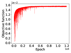
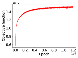
Refer to caption
(a) lr=1e5𝑙𝑟1𝑒5lr=1e-5
Refer to caption
(b) lr=1e6𝑙𝑟1𝑒6lr=1e-6
Refer to caption
(c) Relative difference of H𝐻H
Figure A-2: (a-b) Curves of objective function in Eq. (6) under learning rates lr=1e5𝑙𝑟1𝑒5lr=1e-5 and lr=1e6𝑙𝑟1𝑒6lr=1e-6 with ϵ=1e5italic-ϵ1𝑒5\epsilon=1e-5. (c) Relative difference of H𝐻H in training. The relative difference of H𝐻H is defined as HiHi+Δp,qHip,qsubscriptnormsuperscript𝐻𝑖superscript𝐻𝑖Δ𝑝𝑞subscriptnormsuperscript𝐻𝑖𝑝𝑞\frac{\|H^{i}-H^{i+\Delta}\|_{p,q}}{\|H^{i}\|_{p,q}}, where the norm Hp,q=[𝔼p𝔼qH(𝐱,𝐲)2]1/2subscriptnorm𝐻𝑝𝑞superscriptdelimited-[]subscript𝔼𝑝subscript𝔼𝑞𝐻superscript𝐱𝐲212\|H\|_{p,q}=\left[\mathbb{E}_{p}\mathbb{E}_{q}H(\mathbf{x},\mathbf{y})^{2}\right]^{1/2} (i.e., the L2subscript𝐿2L_{2}-norm of functions on the sample space associated to measure pqtensor-product𝑝𝑞p\otimes q). Hisuperscript𝐻𝑖H^{i} is the function at training step i𝑖i. To reduce the computational cost, we set Δ=10000Δ10000\Delta=10000. p𝑝p and q𝑞q are distributions of source and target training data.
On the choice of ϵitalic-ϵ\epsilon.

To better approach the original OT in Eqs. (2-3) by the L2subscript𝐿2L_{2}-regularized OT in Eq. (5) so that the OT guidance could be better achieved, the ϵitalic-ϵ\epsilon should be small. However, due to the term 1ϵ1italic-ϵ\frac{1}{\epsilon} in the objective function in Eq. (6), smaller ϵitalic-ϵ\epsilon may suffer from numerical issues in training. As a balance, we empirically choose a ϵitalic-ϵ\epsilon from candidate values 1e-5, 1e-6, 1e-7 such that the training is more stable. We show the objective function curves under varying ϵitalic-ϵ\epsilon in Fig. A-3. The training curves seem to be stable in general. We have also reported the results with varying ϵitalic-ϵ\epsilon in Table A-3. From Table A-3, we can see that FID ranges in [13.68, 14.56] (which seems to be stable) for ϵitalic-ϵ\epsilon in [1e-7,1e-3]. We can also see that Acc is similar for ϵitalic-ϵ\epsilon in 1e-7, 1e-6,1e-5, and decreases as ϵitalic-ϵ\epsilon increases from 1e-5 to 1e-3.

Refer to caption
(a) ϵ=1e5italic-ϵ1𝑒5\epsilon=1e-5
Refer to caption
(b) ϵ=1e6italic-ϵ1𝑒6\epsilon=1e-6
Refer to caption
(c) ϵ=1e7italic-ϵ1𝑒7\epsilon=1e-7
Figure A-3: The curves of objective function in training under varying ϵitalic-ϵ\epsilon with learning rate lr=1e6𝑙𝑟1𝑒6lr=1e-6.
Table A-3: Results of OTCS using varying ϵitalic-ϵ\epsilon.
ϵitalic-ϵ\epsilon 1e-7 1e-6 1e-5 1e-4 1e-3
FID \downarrow 14.56 14.12 13.68 13.52 13.91
Acc \uparrow 95.11 96.00 96.44 90.22 77.78
Computational cost.

We report the computational time cost of our training process in this paragraph. As illustrated in Algorithm 2 in the Appendix A, our method consists of three processes in training: (1) learning the potentials uωsubscript𝑢𝜔u_{\omega} & vωsubscript𝑣𝜔v_{\omega}, (2) computing H𝐻H & storing the target sample indexes with non-zero H(H>0.001)𝐻𝐻0.001H(H>0.001) for each source sample, and (3) training the score-based model sθsubscript𝑠𝜃s_{\theta}. We report the computational time cost of these three processes in the following Table A-4.

Table A-4: Computational time cost of training processes.
Dataset Learning uωsubscript𝑢𝜔u_{\omega} & vωsubscript𝑣𝜔v_{\omega} (30w steps) Computing & storing H𝐻H Training sθsubscript𝑠𝜃s_{\theta} (60w steps)
CelebA 3.5 hours 0.5 hours 5 days
Animal 2.0 hours 0.05 hours 5 days

From Table A-4, we can see that (1) learning uωsubscript𝑢𝜔u_{\omega} & vωsubscript𝑣𝜔v_{\omega} and (2) computing & storing H𝐻H takes no more than 4 hours. Similarly to the other diffusion approaches, (3) training our score-based model sθsubscript𝑠𝜃s_{\theta} takes a few days.
Computational time of each operation in a single step of training sθsubscriptsθs_{\theta}. In each step of training the score-based model sθsubscript𝑠𝜃s_{\theta}, we sequentially (1) sampling the index of target sample with probability proportional to H𝐻H for a randomly selected source sample index (sampling index), then (2) load corresponding images (loading image), and (3) finally feed data to network and update model parameters (updating network). Compared with the training of score-based model for paired setting, our training additionally contains the operation of sampling index. From Table A-5, we can see that sampling index takes much less time than updating network.

Table A-5: Computational time of operations in a single step of training sθsubscript𝑠𝜃s_{\theta} on Animal dataset.
Sampling index Loading image Updating network
0.0005 seconds 0.01 seconds 0.7 seconds

D.2 Additional Results on Toy Data Experiments

Results of OTCS under varying ϵitalic-ϵ\epsilon. We show the results of OTCS under varying ϵitalic-ϵ\epsilon in Fig. A-4. We can see that the histogram of generated samples by OTCS fits the estimated conditional transport plan when ϵitalic-ϵ\epsilon is 0.01, 0.001, and 0.0001.

Refer to caption
(a) ϵ=0.1italic-ϵ0.1\epsilon=0.1
Refer to caption
(b) ϵ=0.01italic-ϵ0.01\epsilon=0.01
Refer to caption
(c) ϵ=0.001italic-ϵ0.001\epsilon=0.001
Figure A-4: The histogram (“hist”) of generated samples by our proposed OTCS and the estimated conditional transport plan π^(𝐲|4)^𝜋conditional𝐲4\hat{\pi}(\mathbf{y}|-4) under varying ϵitalic-ϵ\epsilon.

Results of OTCS under varying conditions. We show the results of OTCS for varying condition 𝐱𝐱\mathbf{x} in Fig. A-5. We can see that the histogram of generated samples by OTCS fits the estimated conditional transport plan for 𝐱=5,4,3𝐱543\mathbf{x}=-5,-4,-3.

Refer to caption
(a) 𝐱=5𝐱5\mathbf{x}=-5
Refer to caption
(b) 𝐱=4𝐱4\mathbf{x}=-4
Refer to caption
(c) 𝐱=3𝐱3\mathbf{x}=-3
Figure A-5: The histogram (“hist”) of generated samples by our proposed OTCS and the estimated conditional transport plan π^(𝐲|𝐱)^𝜋conditional𝐲𝐱\hat{\pi}(\mathbf{y}|\mathbf{x}) under varying condition 𝐱𝐱\mathbf{x}. ϵ=0.0001italic-ϵ0.0001\epsilon=0.0001 in this experiment.

D.3 Additional Results in Unpaired Super-Resolution

Results of different methods in unpaired super-resolution.

In Figs. A-6 and A-7, we visualize the translated images by our proposed OTCS, adversarial training-based OT methods of NOT and KNOT, and diffusion-based methods of SCONES, EGSDE, and DDIB. We can see that OTCS, NOT, and KNOT better preserve the identity/structure than SCONES, EGSDE, and DDIB. OTCS produces clearer translated images than NOT. The translated images by KNOT have artifacts (please zoom in on the figure to see the artifacts).
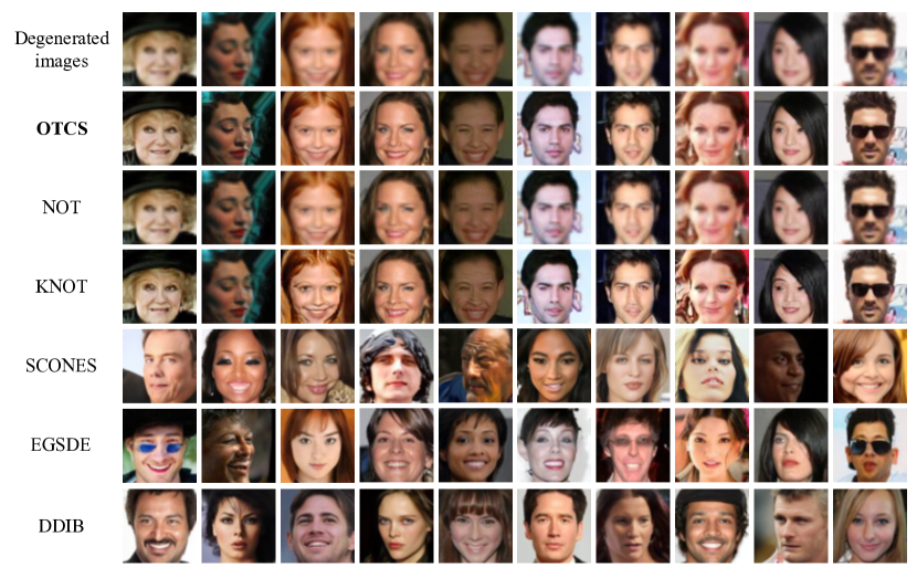
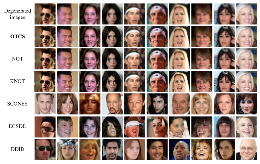
Refer to caption
Figure A-6: Translated images by our proposed OTCS, adversarial training-based OT methods of NOT and KNOT, and diffusion-based methods of SCONES, EGSDE, and DDIB.
Refer to caption
Figure A-7: Translated images by our proposed OTCS, adversarial training-based OT methods of NOT and KNOT, and diffusion-based methods of SCONES, EGSDE, and DDIB.
Refer to caption
Figure A-8: Translated images by SCONES and OTCS with different initialization in inference. We consider the following initialization strategies: 1) We sample a noisy data 𝐲Msubscript𝐲𝑀\mathbf{y}_{M} from pM|0(𝐲M|𝐱)subscript𝑝conditional𝑀0conditionalsubscript𝐲𝑀𝐱p_{M|0}(\mathbf{y}_{M}|\mathbf{x}) as initial state, and the reverse SDE starts at time M𝑀M. 𝐱𝐱\mathbf{x} is the degenerated image and M𝑀M is set to 0.2, 0.4, 0.8, and 1.0; 2) We directly generate a random noise 𝐲Tsubscript𝐲𝑇\mathbf{y}_{T} from 𝒩(0,𝐈)𝒩0𝐈\mathcal{N}(0,\mathbf{I}) as initial state (denoted as “Rand”).
Translated images by SCONES and OTCS with different initial strategies in reverse SDE in inference.

We show the translated images of SCONES and our proposed OTCS in Fig. A-8 with different initialization strategies in inference. We can observe that for the smaller initial noise scales (0.2 and 0.4), the translated images by SCONES are not realistic. For larger initial noise scales (0.8 and 1.0), the structures of translated images by SCONES are apparently different from those of degenerated images. The translated images by OTCS seem to be more realistic and share better structure similarity to degenerated images than SCONES, under different initial noise scales.

D.4 Additional Results in Semi-paired I2I

Translated animal images by different methods.

We provide translated animal images by different methods in Figs. A-9A-10, and A-11. We can see that OTCS better translates the source images to high-quality target images of desired species than the other methods.
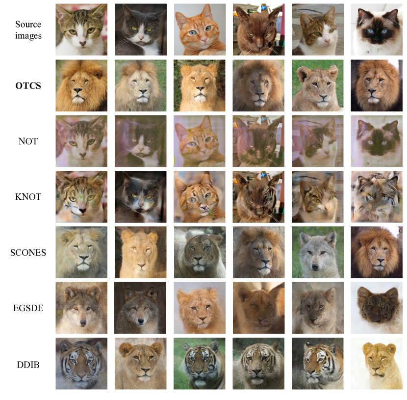
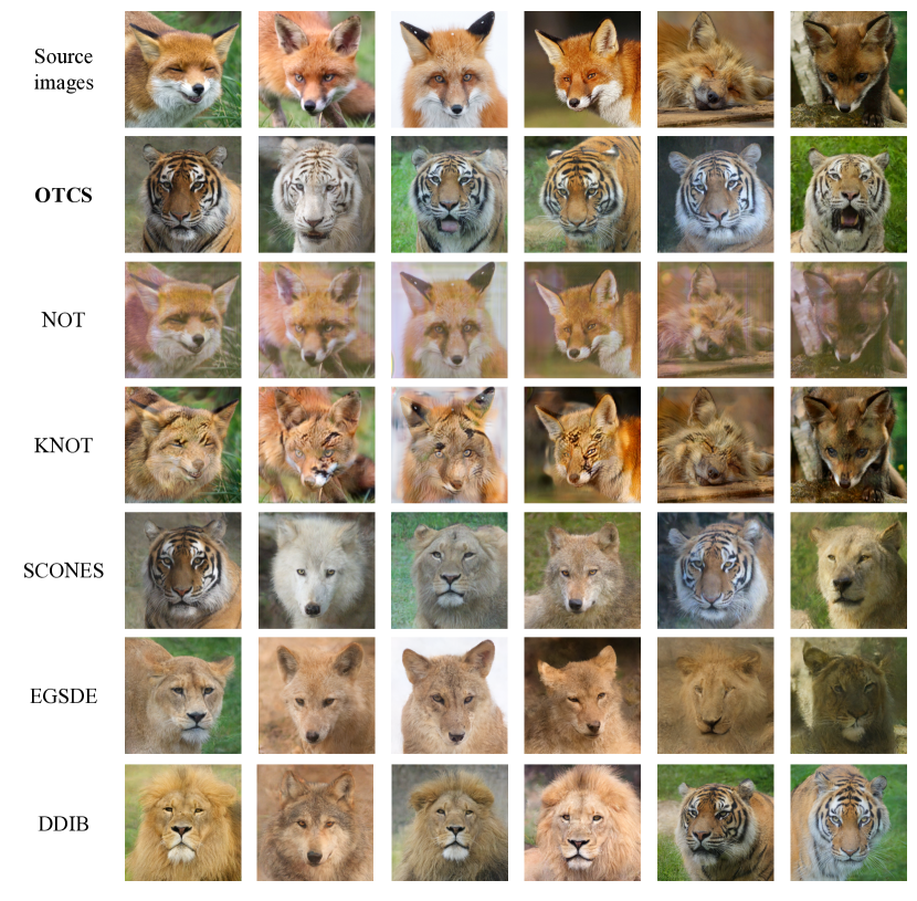
Refer to caption
Figure A-9: Translated images of cat by different methods. With the guidance of paired images, we expect the images of cat to be translated into images of lion.
Refer to caption
Figure A-10: Translated images of fox by different methods. With the guidance of paired images, we expect the images of fox to be translated into images of tiger.
Refer to caption
Figure A-11: Translated images of leopard by different methods. With the guidance of paired images, we expect the images of leopard to be translated into images of wolf.

D.5 Results for Trained Models at Different Training Steps

In Figs. A-12A-13, and A-14, we show the translated images by OTCS in unpaired super-resolution using trained models at varying training steps, in which we consider different initial time M𝑀M in reverse SDE for generating samples.

Refer to caption
Figure A-12: Translated images by OTCS using models at varying training steps, in which we consider different initial time in reverse SDE for generating samples.
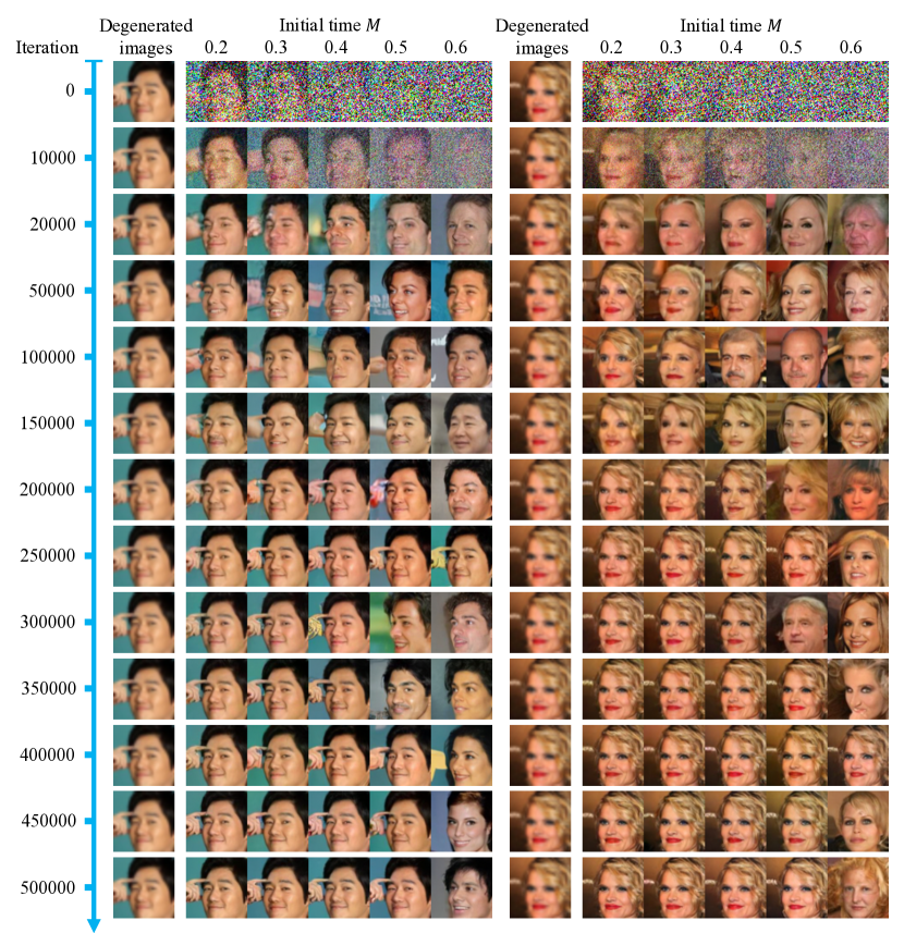
Refer to caption
Figure A-13: Translated images by OTCS using trained models at varying training steps, in which we consider different initial time in reverse SDE for generating samples.
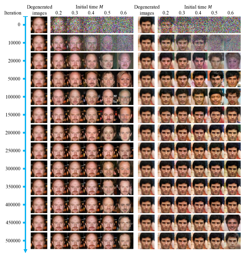
Refer to caption
Figure A-14: Translated images by OTCS using models at varying training steps, in which we consider different initial time in reverse SDE for generating samples.