Combating Inter-Operator Pilot Contamination in Reconfigurable Intelligent Surfaces Assisted Multi-Operator Networks

Abstract

In this paper, we study a new kind of pilot contamination appearing in multi-operator reconfigurable intelligent surfaces (RIS) assisted networks, where multiple operators provide services to their respective served users. The operators use dedicated frequency bands, but each RIS inadvertently reflects the transmitted uplink signals of the user equipment devices in multiple bands. Consequently, the concurrent reflection of pilot signals during the channel estimation phase introduces a new inter-operator pilot contamination effect. We investigate the implications of this effect in systems with either deterministic or correlated Rayleigh fading channels, specifically focusing on its impact on channel estimation quality, signal equalization, and channel capacity. The numerical results demonstrate the substantial degradation in system performance caused by this phenomenon and highlight the pressing need to address inter-operator pilot contamination in multi-operator RIS deployments. To combat the negative effect of this new type of pilot contamination, we propose to use orthogonal RIS configurations during uplink pilot transmission, which can mitigate or eliminate the negative effect of inter-operator pilot contamination at the expense of some inter-operator information exchange and orchestration.

I Introduction

Pilot contamination is a key problem that frequently arises in wireless communication systems [2]. When multiple users use the same pilot sequences simultaneously in the same band, due to the limited channel coherence time, the base station (BS) cannot distinguish their channels. This typically results in poor channel estimates and extra beamformed interference from or towards the user equipments that reuse the same pilot sequence. Therefore, pilot contamination adversely affects the coherent reception of data, and methods to mitigate pilot contamination—including adaptive pilot reuse, power control, user grouping, multi-cell coordination, and coded random access techniques—have been widely studied in the communication literature [2, 3, 4, 5, 6].

In recent years, reconfigurable intelligent surfaces have arisen as a new technology component for 6G [7]. An RIS is a surface consisting of multiple reflecting elements that have sub-wavelength spacing and controllable reflection properties [8]. This feature provides partial control of the propagation environment that can lead to better services for users, especially when their serving BS is not in their line of sight (LOS). By adjusting the impedances of the individual elements via a RIS controller, the elements are capable of adding desired phase shifts to the reflected signals, thereby forming reflected beams in desired directions that can significantly boost the signal-to-interference-plus-noise ratio (SINR) and reduce the symbol estimation error at the receiver [7, 9].

On the other hand, the addition of RISs to existing systems introduces new design and operational challenges [10]. For example, the length of the pilot signal required by a single UE is proportional to the number of RIS elements (e.g., tens or hundreds), because the RIS must change its configuration to explore all channel dimensions [11, 12]. In addition, the path loss of the reflected path through a passive RIS is proportional to the multiplication of the path losses to and from the RIS [13], so a larger surface is needed to achieve a decent signal-to-noise ratio (SNR) improvement. Active RISs, on the other hand, use amplifiers to overcome the large path loss but have the traditional issues of relays: increased power consumption, higher cost, and additional noise [14, 15]. While the aforementioned problems caused by the RIS have been recognized [16], pilot contamination caused by the presence of multiple RISs has not been studied in the literature.

Wireless communication systems use standardized protocols, interfaces, and well-defined pilot sequences and codebooks to ensure inter-operability [17]. While employing RISs in cellular networks have not been studied by the relevant standards organizations yet, it may be expected that the configuration sequences that facilitate the deployment of RISs while maintaining interoperability will be specified. Consequently, when multiple cellular networks are deployed by different network operators in overlapping geographical areas, the RISs may adopt identical or overlapping pilot sequences and cause pilot contamination. The number of orthogonal pilot sequences is limited by the length of the pilot sequence, and increasing the pilot sequence length not only creates more channel estimation overhead but also is infeasible due to the limited coherence budget of the channel. As a consequence, the need for repeating pilot sequences comes up very often.

In this paper, we argue that when multiple RISs are deployed for the purpose of shaping the propagation characteristics of the environment, the propagation characteristics might change in unintended ways. For example, an RIS belonging to another operator might modify the propagation of a UE’s own pilot signal, leading to pilot contamination even in the absence of any interfering signals or intra-band pilot reuse. The underlying reason is that an RIS element—although designed for a particular frequency—does not act as a bandpass filter, but reflects all frequencies with varying amplitude and phase. Indeed, as pointed out in [18], due to the lack of baseband signal processing, the RIS reflects the impinging broadband signal with frequency-flat reflection coefficients. Therefore, in realistic system models of, for example, passive RIS assisted 5G New Radio systems, we need to take into account that the RIS inadvertently reflects the transmitted uplink signals of the user equipment devices in multiple bands as in [19], [20].

Specifically, in this paper, we identify this new pilot contamination phenomenon as a major practical challenge when multiple RIS assisted operator networks are deployed over a geographical area, including the important practical scenario of inter-operator site sharing [21, 22]. In such an environment, a UE that transmits pilots to its serving BS via multiple RIS, which may change their configurations simultaneously, is exposed to new pilot-related ambiguities that have not been studied before. Since this phenomenon exacerbates the pilot contamination problem, it is clear that pilot contamination due to the presence of multiple RISs must be dealt with.

To the best of the authors’ knowledge, the problem of inter-operator pilot contamination in RIS-aided wireless communication systems has not been addressed before, except in the preliminary version of this manuscript [1], which assumed deterministic rather than stochastically fading channels. In this paper, we derive the capacity lower bound of the system under pilot contamination and imperfect channel state information (CSI) assuming Rayleigh fading. Our major contributions can be summarized as follows:

• For the case when inter-operator pilot contamination is neglected, we provide a misspecified maximum likelihood (ML) estimator under the assumption that all the channels in the system setup are deterministic. We also derive the resulting channel estimation mean squared error (MSE) for different choices of the RIS configurations.

• Based on the obtained results for the channel estimation error under inter-operator pilot contamination, we provide the data signal estimation MSE for a misspecified minimum mean squared error (MMSE) estimator.

• In addition to deterministic channels, we also consider the case where the channels are Rayleigh fading with spatial correlation. For generic channel spatial covariances, we derive the misspecified MMSE estimator and the resulting MSE.

• Based on the channel estimation error model, obtained for spatially correlated Rayleigh fading channels, we derive a capacity lower bound given the channel estimates. Our numerical results show that the choice of RIS configurations during channel estimation makes a significant impact on the capacity lower bound.

The rest of the manuscript is organized as follows: in Section II, we provide the received signal model, in Section III, we provide the misspecified ML estimator where the inter-operator pilot contamination is neglected and the channels are assumed to be deterministic. Section IV builds on top of section III by providing the data estimation MSE as a result of inter-operator pilot contamination. In Section V, we derive the impact of inter-operator pilot contamination in closed-form for the case of spatially correlated Rayleigh-fading channels by considering the channel estimation MSE as our performance metric. Since the data estimation MSE has a dependence on individual channel realizations, an alternative performance metric for data transmission is needed to capture the behavior of fading channels. To this end, we derive the capacity lower bound under channel side information in Section VI. We provide the numerical results in Section VII, and conclude the manuscript in Section VIII.

II System Model

In this paper, we study the pilot contamination caused by the presence of multiple RISs by considering the uplink of a system consisting of two wide-band RISs, two single-antenna UEs, and two co-located single-antenna BSs. The UEs are subscribed to different operators and use non-overlapping frequency bands. Each RIS is dedicated to and controlled by a single operator, but both UE signals are reflected from both RISs. In this scenario, although there is no interference between the two UEs, both RISs affect both frequency bands.

In Fig. 1, we graphically describe the system that we consider. The components associated with the two different operators are depicted in two different colors: blue BS, RIS, UE and the channels belong to operator 1, while the red ones belong to operator 2. The operators can potentially use site-sharing (as in the figure) to reduce deployment costs but transmit over two disjoint narrow frequency bands to their respective serving BSs. Each RIS has $N$ reflecting elements, and is dedicated to and controlled by a single operator but affects both bands. To focus on the fundamentals of pilot contamination, we consider an environment where the direct UE-BS paths are blocked, while the UE-RIS and RIS-BS paths are operational. Since the BSs and RISs have fixed deployment locations, we assume the RIS-BS channels $\mathbf{h}_{k}\in\mathbb{C}^{N}$ are known, while the UE-RIS channels $\mathbf{g}_{k}\in\mathbb{C}^{N}$ are unknown and to be estimated, for $k=1,2$.

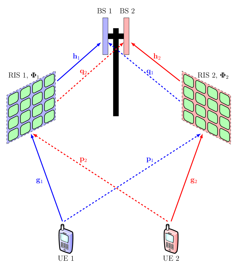
Figure 1: The considered setup with two UEs, two RISs, and two co-located single-antenna BSs. The blue channels correspond to frequency band 1, and the red channels correspond to frequency band 2, subscribed by UEs $1$ and $2$, respectively. The desired channels are denoted by solid lines, while the undesired channels (whose existences might be unknown to the BSs) are denoted by dashed lines. Each channel vector is $N$-dimensional because each RIS has $N$ elements.

The signal transmitted by UE $k$ reaches its serving BS through the channels $\mathbf{h}_{k}$ and $\mathbf{g}_{k}$, for $k=1,2$. Importantly, each UE’s transmitted signal is also reflected by the non-serving operator’s RIS and parts of the reflected signal will reach the serving BS. This effect contaminates the pilot signal reflected by the serving RIS and we will study the implications. The phenomenon is illustrated in Fig. 1, where the resulting UE-RIS and RIS-BS channels are denoted by $\mathbf{p}_{k}\in\mathbb{C}^{N}$ and $\mathbf{q}_{k}\in\mathbb{C}^{N}$, respectively, for $k=1,2$. Defining the pilot signal of UE $k$ as $s_{k}\in\mathbb{C}$, the received signals on bands $1$ and $2$ at the BSs can be expressed as

$$y_{p1}=\sqrt{P_{p}}\mathbf{h}_{1}^{T}\boldsymbol{\Phi}_{1}\mathbf{g}_{1}s_{1}+\sqrt{P_{p}}\mathbf{q}_{1}^{T}\boldsymbol{\Phi}_{2}\mathbf{p}_{1}s_{1}+w_{p1},$$ (1a)

$$y_{p2}=\sqrt{P_{p}}\mathbf{h}_{2}^{T}\boldsymbol{\Phi}_{2}\mathbf{g}_{2}s_{2}+\sqrt{P_{p}}\mathbf{q}_{2}^{T}\boldsymbol{\Phi}_{1}\mathbf{p}_{2}s_{2}+w_{p2},$$ (1b)

where $y_{pk}\in\mathbb{C}$ denotes the received signal, $w_{pk}\sim\mathcal{CN}(0,1)$ denotes the receiver noise for band $k$, and $\boldsymbol{\Phi}_{k}=\text{diag}(e^{-j\phi_{k1}},\dots,e^{-j\phi_{kN}})$ denotes the $k$th RIS’s reflection matrix, and $P_{p}$ denotes the pilot signal’s transmission power. We assume $s_{1}=s_{2}=1$ without loss of generality. When analyzing channel estimation, it is more convenient to rewrite (1) as

$$y_{p1}=\sqrt{P_{p}}\boldsymbol{\phi}_{1}^{T}\mathbf{D}_{\mathbf{h}_{1}}\mathbf{g}_{1}+\sqrt{P_{p}}\boldsymbol{\phi}_{2}^{T}\mathbf{D}_{\mathbf{q}_{1}}\mathbf{p}_{1}+w_{p1},$$ (2a)

$$y_{p2}=\sqrt{P_{p}}\boldsymbol{\phi}_{2}^{T}\mathbf{D}_{\mathbf{h}_{2}}\mathbf{g}_{2}+\sqrt{P_{p}}\boldsymbol{\phi}_{1}^{T}\mathbf{D}_{\mathbf{q}_{2}}\mathbf{p}_{2}+w_{p2},$$ (2b)

where $\mathbf{D}_{\mathbf{h}_{k}}$ and $\mathbf{D}_{\mathbf{q}_{k}}$ represent the $N\times N$ diagonal matrices containing the elements of $\mathbf{h}_{k}$ and $\mathbf{q}_{k}$, and $\boldsymbol{\phi}_{k}\in\mathbb{C}^{N}$ denotes the column vectors containing the diagonal entries of $\boldsymbol{\Phi}_{k}$ for $k=1,2$.

As there are $N$ parameters in $\mathbf{g}_{1}$ and $\mathbf{g}_{2}$, at least $N$ linearly independent observations are needed to estimate them uniquely. To this end, we perform $L\geq N$ pilot transmissions over time, and we vertically stack the received signals to obtain

$$\mathbf{y}_{p1}=\sqrt{P_{p}}\mathbf{B}_{1}\mathbf{D}_{\mathbf{h}_{1}}\mathbf{g}_{1}+\sqrt{P_{p}}\mathbf{B}_{2}\mathbf{D}_{\mathbf{q}_{1}}\mathbf{p}_{1}+\mathbf{w}_{p1},$$ (3a)

$$\mathbf{y}_{p2}=\sqrt{P_{p}}\mathbf{B}_{2}\mathbf{D}_{\mathbf{h}_{2}}\mathbf{g}_{2}+\sqrt{P_{p}}\mathbf{B}_{1}\mathbf{D}_{\mathbf{q}_{2}}\mathbf{p}_{2}+\mathbf{w}_{p2},$$ (3b)

where $\mathbf{y}_{pk}=[y_{pk}[1],\dots,y_{pk}[L]]^{T}\in\mathbb{C}^{L}$ denotes the sequence of received signals from the $k$th UE over $L$ time instances, and the matrices $\mathbf{B}_{1}$ and $\mathbf{B}_{2}$ represent the sequence of RIS configurations over $L$ time instances; that is, $\mathbf{B}_{k}\triangleq\begin{bmatrix}\boldsymbol{\phi}_{k}[1]&\dots&\boldsymbol{\phi}_{k}[L]\end{bmatrix}^{T}\in\mathbb{C}^{L\times N}$ for $k=1,2$.

In the remainder of this paper, we will analyze channel estimation and the resulting communication performance for deterministic and fading channels, respectively.

III Maximum Likelihood Estimation of Deterministic Channels

In this section, we will consider channel estimation for deterministic channels. The same assumptions and results will then be considered in Section IV for data transmission.

We assume that $\mathbf{g}_{k}$ is a deterministic and unknown channel without any known structure. That is, $\mathbf{g}_{k}$ is an $N\times 1$ vector of complex deterministic parameters to be estimated. In addition, we assume that $\mathbf{h}_{k}$ is perfectly known. On the other hand, the BSs do not know the existence of $\mathbf{q}_{k}$ and $\mathbf{p}_{k}$. Consequently, we can denote the received signal models assumed by the BSs as

$$\hat{\mathbf{y}}_{p1}=\sqrt{P_{p}}\mathbf{B}_{1}\mathbf{D}_{\mathbf{h}_{1}}\mathbf{g}_{1}+\mathbf{w}_{p1},$$ (4a)

$$\hat{\mathbf{y}}_{p2}=\sqrt{P_{p}}\mathbf{B}_{2}\mathbf{D}_{\mathbf{h}_{2}}\mathbf{g}_{2}+\mathbf{w}_{p2}.$$ (4b)

Since $\mathbf{g}_{k}$ does not have a known structure and hence consists of $N$ scalars, BS $k$ requires at least $N$ independent observations to estimate it. To this end, both $\mathbf{B}_{1},\mathbf{B}_{2}\in\mathbb{C}^{L\times N}$ must have full column rank. Furthermore, we require that the RIS configurations used at different time instances are mutually orthogonal and contain entries on the unit circle that can be realized using a reflecting element. These assumptions result in $\mathbf{B}_{k}^{H}\mathbf{B}_{k}=L\mathbf{I}_{N}$. In classical non-Bayesian parameter estimation, the ML estimator is widely used, which maximizes the likelihood function of the received observation over the unknown parameter. Since the BSs have misspecified received pilot signal models, they will instead maximize the likelihood functions obtained from the misspecified model, leading to misspecified maximum likelihood (MML) estimators. For (4), the MML estimator can be expressed as

$$\hat{\mathbf{g}}_{k} =\arg\max_{\mathbf{g}_{k}}f(\mathbf{y}_{pk};\mathbf{g}_{k})$$

$$=\arg\max_{\mathbf{g}_{k}}\frac{1}{(\pi\sigma_{w}^{2})^{L}}\exp{\left(-\frac{\|\mathbf{y}_{pk}-\sqrt{P_{p}}\mathbf{B}_{k}\mathbf{D}_{\mathbf{h}_{k}}\mathbf{g}_{k}\|^{2}}{\sigma_{w}^{2}}\right)}$$

$$=\arg\min_{\mathbf{g}_{k}}\left\|\mathbf{y}_{pk}-\sqrt{P_{p}}\mathbf{B}_{k}\mathbf{D}_{\mathbf{h}_{k}}\mathbf{g}_{k}\right\|^{2}$$

$$=\frac{1}{\sqrt{P_{p}}}\mathbf{D}_{\mathbf{h}_{k}}^{-1}(\mathbf{B}_{k}^{H}\mathbf{B}_{k})^{-1}\mathbf{B}_{k}^{H}\mathbf{y}_{pk}$$

$$=\frac{1}{L\sqrt{P_{p}}}\mathbf{D}_{\mathbf{h}_{k}}^{-1}\mathbf{B}_{k}^{H}\mathbf{y}_{pk}.$$ (5)

In the following subsections, we describe the behavior of this estimator for two different choices of the $\mathbf{B}_{k}$ matrices.

III-A Case 1: The RISs Adopt the Same Configuration Sequence

We discussed in the introduction that in the absence of inter-operator cooperation, it is highly likely that the RISs will use the same standardized sequence of configurations during the channel estimation phase, which corresponds to $\mathbf{B}_{1}=\mathbf{B}_{2}=\mathbf{B}$. In this case, (5) becomes

$$\hat{\mathbf{g}}_{k}=\mathbf{g}_{k}+\mathbf{D}_{\mathbf{h}_{k}}^{-1}\mathbf{D}_{\mathbf{q}_{k}}\mathbf{p}_{k}+\frac{1}{L\sqrt{P}_{p}}\mathbf{D}_{\mathbf{h}_{k}}^{-1}\mathbf{B}^{H}\mathbf{w}_{pk}.$$ (6)

Since we consider the channels as deterministic parameters, we obtain the probability distribution

$$\hat{\mathbf{g}}_{k}\sim\mathcal{CN}\!\left(\mathbf{g}_{k}+\mathbf{D}_{\mathbf{h}_{k}}^{-1}\mathbf{D}_{\mathbf{q}_{k}}\mathbf{p}_{k},\frac{\sigma_{w}^{2}}{LP_{p}}(\mathbf{D}_{\mathbf{h}_{k}}^{H}\mathbf{D}_{\mathbf{h}_{k}})^{-1}\!\right).$$ (7)

We notice that $\hat{\mathbf{g}}_{k}$ is biased; that is, $\mathbf{b}_{k}\triangleq\mathbb{E}[\hat{\mathbf{g}}_{k}-\mathbf{g}_{k}]=\mathbf{D}_{\mathbf{h}_{k}}^{-1}\mathbf{D}_{\mathbf{q}_{k}}\mathbf{p}_{k}\neq\boldsymbol{0}$. The estimator bias does not vanish when increasing $P_{p}$ or $L$, or decreasing $\sigma_{w}^{2}$. Hence, this estimator is not asymptotically unbiased. This is a new instance of an extensively studied phenomenon in the massive multiple-input multiple-output (MIMO) literature, namely pilot contamination [2, 3]. Interestingly, the RISs cause pilot contamination even between two non-overlapping frequency bands, which has not been recognized in the previous literature.

III-B Case 2: The RISs Adopt Different Configuration Sequences

In this section, we consider the generic case of $\mathbf{B}_{1}\neq\mathbf{B}_{2}$. To motivate the proposed method for configuring $\mathbf{B}_{1}$ and $\mathbf{B}_{2}$, we first consider the case where the BSs are aware of the true signal model in (3), and therefore can estimate both $\mathbf{g}_{k}$ and $\mathbf{r}_{k}\triangleq\mathbf{D}_{\mathbf{q}_{k}}\mathbf{p_{k}}$. The resulting system model can be expressed as

$$\mathbf{y}_{p1}=\sqrt{P}_{p}\begin{bmatrix}\mathbf{B}_{1}\mathbf{D}_{\mathbf{h}_{1}}&\mathbf{B}_{2}\end{bmatrix}\begin{bmatrix}\mathbf{g}_{1}\\ \mathbf{r}_{1}\end{bmatrix}+\mathbf{w}_{p1},$$ (8a)

$$\mathbf{y}_{p2}=\sqrt{P}_{p}\begin{bmatrix}\mathbf{B}_{2}\mathbf{D}_{\mathbf{h}_{2}}&\mathbf{B}_{1}\end{bmatrix}\begin{bmatrix}\mathbf{g}_{2}\\ \mathbf{r}_{2}\end{bmatrix}+\mathbf{w}_{p2}.$$ (8b)

In (8), a known linear transformation is applied to the parameter vector of interest in the presence of additive noise. Consequently, the ML estimates of UE 1’s channels become

$$\begin{bmatrix}\hat{\mathbf{g}}_{1}\\ \hat{\mathbf{r}}_{1}\end{bmatrix}=\frac{1}{\sqrt{P_{p}}}\begin{bmatrix}L\mathbf{D}_{\mathbf{h}_{1}}^{H}\mathbf{D}_{\mathbf{h}_{1}}&\mathbf{D}_{\mathbf{h}_{1}}^{H}\mathbf{B}_{1}^{H}\mathbf{B}_{2}\\ \mathbf{B}_{2}^{H}\mathbf{B}_{1}\mathbf{D}_{\mathbf{h}_{1}}&L\mathbf{I}_{N}\end{bmatrix}^{-1}\begin{bmatrix}\mathbf{D}_{\mathbf{h}_{1}}^{H}\mathbf{B}_{1}^{H}\\ \mathbf{B}_{2}^{H}\end{bmatrix}\mathbf{y}_{p1}.$$ (9)

Note that in this case, the total dimension of the unknown parameter vector is $2N$, hence, at least $2N$ independent observations are required for the matrix inverse to exist. The structure in (9) applies to UE 2 with alternated indices, and it gives the ML estimator, which is both unbiased and efficient, since (8) is a linear observation model with additive Gaussian noise [23, Th. 7.3]. Hence, (9) is unbiased irrespective of other parameters such as $\sigma_{w}^{2}$, $L$, and $P_{p}$, and it achieves the Cramér-Rao Lower Bound (CRLB), which provides a lower bound on the MSE of any unbiased estimator [24]. It has to be noted that when $\mathbf{B}_{1}^{H}\mathbf{B}_{2}=\boldsymbol{0}$, (9) becomes

$$\begin{bmatrix}\hat{\mathbf{g}}_{1}\\ \hat{\mathbf{r}}_{1}\end{bmatrix} =\frac{1}{L\sqrt{P_{p}}}\begin{bmatrix}\mathbf{D}_{\mathbf{h}_{1}}^{H}\mathbf{D}_{\mathbf{h}_{1}}&\boldsymbol{0}\\ \boldsymbol{0}&\mathbf{I}_{N}\end{bmatrix}^{-1}\begin{bmatrix}\mathbf{D}_{\mathbf{h}_{1}}^{H}\mathbf{B}_{1}^{H}\\ \mathbf{B}_{2}^{H}\end{bmatrix}\mathbf{y}_{p1}$$

$$=\frac{1}{L\sqrt{P_{p}}}\begin{bmatrix}\mathbf{D}_{\mathbf{h}_{1}}^{-1}\mathbf{B}_{1}^{H}\\ \mathbf{B}_{2}^{H}\end{bmatrix}\mathbf{y}_{p1}.$$ (10)

Note that the expression for $\hat{\mathbf{g}}_{1}$ in (III-B) is the same as in (5). This shows that when $\mathbf{B}_{1}^{H}\mathbf{B}_{2}=\boldsymbol{0}$, the MML in (5) coincides with the ML estimator; that is, the misspecified model is sufficient when the configuration sequences are designed to alleviate pilot interference because the missing terms anyway vanish in the receiver processing. The probability distribution of $\hat{\mathbf{g}}_{k}$ in this case can be expressed as

$$\hat{\mathbf{g}}_{k}\sim\mathcal{CN}\left(\mathbf{g}_{k},\frac{\sigma_{w}^{2}}{LP_{p}}(\mathbf{D}_{\mathbf{h}_{k}}^{H}\mathbf{D}_{\mathbf{h}_{k}})^{-1}\right),$$ (11)

which shows that choosing the RIS configuration sequences such that $\mathbf{B}_{1}$ and $\mathbf{B}_{2}$ remove the bias from the MML estimator. However, the major setback of this approach is that the minimum number of observations required for this channel estimation procedure is $2N$ instead of $N$, due to the fact that the $2N$-many $L$-dimensional columns must all be mutually orthogonal, for which $L\geq 2N$ is required. Considering that the estimator bias in (7) does not vanish with increasing $L$, this is a necessary sacrifice. Hence, it has to be noted that the number of pilot transmissions increases linearly with the number of RISs deployed in proximity.

III-C MSE During Channel Estimation

The estimation error can be quantified through the MSE, which is the trace of the error covariance matrix. We will derive the MSE in this section. In this derivation, we do not assume a particular choice of $\mathbf{B}_{1}$ and $\mathbf{B}_{2}$, but we utilize the basic assumption $\mathbf{B}_{k}\mathbf{B}_{k}^{H}=L\mathbf{I}_{N}$. Consequently, we use $\mathbf{b}_{k}$ to denote the potential estimator bias. We can then compute the error covariance matrix as

$$\boldsymbol{\Sigma}_{e,k} =\mathbb{E}\left[(\hat{\mathbf{g}}_{k}-\mathbf{g}_{k})(\hat{\mathbf{g}}_{k}-\mathbf{g}_{k})^{H}\right]$$

$$=\mathbf{b}_{k}\mathbf{b}_{k}^{H}+\frac{1}{LP_{p}}\mathbb{E}\left[\mathbf{D}_{\mathbf{h}_{k}}^{-1}\mathbf{w}_{pk}\mathbf{w}_{pk}^{H}\mathbf{D}_{\mathbf{h}_{k}}^{-H}\right]$$

$$=\mathbf{b}_{k}\mathbf{b}_{k}^{H}+\frac{\sigma_{w}^{2}}{LP_{p}}\left(\mathbf{D}_{\mathbf{h}_{k}}\mathbf{D}_{\mathbf{h}_{k}}^{H}\right)^{-1}.$$ (12)

Consequently, the trace of the error covariance matrix becomes

$$\mathrm{tr}(\boldsymbol{\Sigma}_{e,k})=\|\mathbf{b}_{k}\|^{2}+\frac{\sigma_{w}^{2}}{LP_{p}}\sum_{n=1}^{N}\frac{1}{|h_{kn}|^{2}}.$$ (13)

Note that for high $P_{p}$, $L$, and/or low $\sigma_{w}^{2}$, the second term in (13) vanishes, and the trace of the error covariance converges to $\|\mathbf{b}_{k}\|^{2}$ which depends on the configurations of $\mathbf{B}_{1},\mathbf{B}_{2}$. For the two previously considered cases, we have

$$\|\mathbf{b}_{k}\|^{2}=\begin{cases}\sum_{n=1}^{N}\frac{|r_{kn}|^{2}}{|h_{kn}|^{2}}&\mathbf{B}_{1}=\mathbf{B}_{2},\\ 0&\mathbf{B}_{1}^{H}\mathbf{B}_{2}=\boldsymbol{0}.\end{cases}$$ (14)

This result shows that configuring the RISs such that $\mathbf{B}_{1}^{H}\mathbf{B}_{2}=\boldsymbol{0}$ removes the asymptotic floor on the average MSE, which comes from the energy of the estimator bias. On the other hand, when the intended RIS-BS links $\mathbf{h}_{1},\mathbf{h}_{2}$ are strong relative to the unintended and unknown overall link $\mathbf{r}_{k}$, the estimator bias will be weaker and the performance loss associated with choosing $\mathbf{B}_{1}=\mathbf{B}_{2}$ will be lower. Nevertheless, pilot contamination results in a fundamental error floor, even if the RISs are utilized in different bands. In the next section, we consider the estimation of data based on the channel estimation performed in this section and analyze the consequence of pilot contamination in this phase.

IV Data Signal Estimation with Deterministic Channels

The channel estimation is followed by data transmission over the same deterministic channel as in Section III. The receiver can use the channel estimate derived in the last section when determining the transmitted signal. Practical channels are never fully deterministic but might have a long coherence time. Moreover, the impact of estimation errors is only relevant when the data packet has a modest size so we cannot afford to spend much resources on pilots. For this reason, we cannot consider the channel capacity as performance metric but will instead consider the MSE.

Defining the data signal transmitted by the $k$th UE as $x_{k}\sim\mathcal{CN}(0,1)$, we can express the received data as

$$y_{1}=\sqrt{P_{d}}(\mathbf{h}_{1}^{T}\hat{\boldsymbol{\Phi}}_{1}\mathbf{g}_{1}+\mathbf{q}_{1}^{T}\hat{\boldsymbol{\Phi}}_{2}\mathbf{p}_{1})x_{1}+w_{1},$$ (15a)

$$y_{2}=\sqrt{P_{d}}(\mathbf{h}_{2}^{T}\hat{\boldsymbol{\Phi}}_{2}\mathbf{g}_{2}+\mathbf{q}_{2}^{T}\hat{\boldsymbol{\Phi}}_{1}\mathbf{p}_{2})x_{2}+w_{2},$$ (15b)

where $w_{k}\sim\mathcal{CN}(0,\sigma_{w}^{2})$ denotes the receiver noise, $P_{d}$ denotes the data transmission power, and the RIS configuration matrices $\hat{\boldsymbol{\Phi}}_{k}$ are selected based on the estimated channels to maximize the average gain of the desired cascaded channel as shown in [12, Sec. II]:

$$\hat{\phi}_{kn}=\arg(h_{kn})+\arg(\hat{g}_{kn}),$$

$$\hat{\boldsymbol{\Phi}}_{k}=\mathrm{diag}\left(e^{-j\hat{\phi}_{k1}},\dots,e^{-j\hat{\phi}_{kN}}\right).$$ (16)

However, since the BSs are unaware of the unintended reflections and base their data reception on the previously obtained channel estimates, they assume the following misspecified received data signal models:

$$\hat{y}_{1}=\sqrt{P_{d}}\mathbf{h}_{1}^{T}\hat{\boldsymbol{\Phi}}_{1}\hat{\mathbf{g}}_{1}x_{1}+w_{1},$$ (17a)

$$\hat{y}_{2}=\sqrt{P_{d}}\mathbf{h}_{2}^{T}\hat{\boldsymbol{\Phi}}_{2}\hat{\mathbf{g}}_{2}x_{2}+w_{2}.$$ (17b)

Introducing the notation $m_{k}\triangleq\sqrt{P_{d}}(\mathbf{h}_{k}^{T}\hat{\boldsymbol{\Phi}}_{k}\mathbf{g}_{k}+\mathbf{q}_{k}^{T}\hat{\boldsymbol{\Phi}}_{j}\mathbf{p}_{k})$ for $j,k\in\{1,2\},j\neq k$, and $\hat{m}_{k}\triangleq\sqrt{P_{d}}\mathbf{h}_{k}^{T}\hat{\boldsymbol{\Phi}}_{k}\hat{\mathbf{g}}_{k}$, (15) and (17) can be expressed as

$$y_{k}=m_{k}x_{k}+w_{k},\quad k=1,2,$$ (18a)

$$\hat{y}_{k}=\hat{m}_{k}x_{k}+w_{k},\quad k=1,2.$$ (18b)

Based on the misspecified observation model in (18b), the BSs estimate $x_{k}$ by using the misspecified MMSE estimator

$$\hat{x}_{k}=\frac{\hat{m}_{k}^{*}}{|\hat{m}_{k}|^{2}+\sigma_{w}^{2}}y_{k},\quad k=1,2.$$ (19)

In this section, we consider the MSE between $x_{k}$ and $\hat{x}_{k}$ as the performance metric for the data transmission. We derive the data estimation MSE for UE $k$ as

$$\mathbb{E}\left[|x_{k}-\hat{x}_{k}|^{2}\right]=1+\mathbb{E}\left[|\hat{x}_{k}|^{2}\right]-2\mathrm{Re}(\mathbb{E}[x_{k}\hat{x}_{k}^{*}])$$

$$=1+\mathbb{E}\left[\frac{|\hat{m}_{k}|^{2}(|m_{k}|^{2}+\sigma_{w}^{2})}{(|\hat{m}_{k}|^{2}+\sigma_{w}^{2})^{2}}\right]$$

$$-2\mathrm{Re}\left(\mathbb{E}\left[\frac{\hat{m}_{k}m_{k}^{*}}{|\hat{m}_{k}|^{2}+\sigma_{w}^{2}}\right]\right)$$

$$=1+\mathbb{E}\left[\frac{|\hat{m}_{k}|^{2}(|m_{k}|^{2}+\sigma_{w}^{2})-2\mathrm{Re}(\hat{m}_{1}m_{1}^{*})(|\hat{m}_{k}|^{2}+\sigma_{w}^{2})}{(|\hat{m}_{k}|^{2}+\sigma_{w}^{2})^{2}}\right]$$

$$=1+\mathbb{E}\left[\frac{|\hat{m}_{k}|^{2}(|m_{k}|^{2}+\sigma_{w}^{2})-2\mathrm{Re}(\hat{m}_{1}m_{1}^{*})(|\hat{m}_{k}|^{2}+\sigma_{w}^{2})}{(|\hat{m}_{k}|^{2}+\sigma_{w}^{2})^{2}}\right]$$

$$+\mathbb{E}\left[\frac{\sigma_{w}^{2}(|m_{k}|^{2}+\sigma_{w}^{2})-\sigma_{w}^{2}(|m_{k}|^{2}+\sigma_{w}^{2})}{(|\hat{m}_{k}|^{2}+\sigma_{w}^{2})^{2}}\right]$$

$$=1+\mathbb{E}\left[\frac{(|\hat{m}_{k}|^{2}+\sigma_{w}^{2})(|m_{k}|^{2}+\sigma_{w}^{2}-2\mathrm{Re}(\hat{m}_{k}m_{k}^{*}))}{(\hat{m}_{k}^{2}+\sigma_{w}^{2})^{2}}\right]$$

$$-\mathbb{E}\left[\frac{\sigma_{w}^{2}(|m_{k}|^{2}+\sigma_{w}^{2})}{(\hat{m}_{k}^{2}+\sigma_{w}^{2})^{2}}\right]$$

$$=\mathbb{E}\left[\frac{|m_{k}-\hat{m}_{k}|^{2}+2\sigma_{w}^{2}}{|\hat{m}_{k}|^{2}+\sigma_{w}^{2}}\right]-\mathbb{E}\left[\frac{\sigma_{w}^{2}(|m_{k}|^{2}+\sigma_{w}^{2})}{(|\hat{m}_{k}|^{2}+\sigma_{w}^{2})^{2}}\right].$$ (20)

Defining $\epsilon_{k}\triangleq m_{k}-\hat{m}_{k}$, (20) can be rewritten as

$$\mathbb{E}[|x_{k}-\hat{x}_{k}|^{2}]=\mathbb{E}\left[\frac{|\epsilon_{k}|^{2}+2\sigma_{w}^{2}}{|m_{k}-\epsilon_{k}|^{2}+\sigma_{w}^{2}}-\frac{\sigma_{w}^{2}(|m_{k}|^{2}+\sigma_{w}^{2})}{(|m_{k}-\epsilon_{k}|^{2}+\sigma_{w}^{2})^{2}}\right].$$ (21)

To examine the impact of pilot contamination on the data estimation performance more clearly, we now consider channel estimation at high SNRs, so that the estimation error only comes from the estimator bias, i.e., pilot contamination. This happens when $L$ or $P_{p}$ is high and/or $\sigma_{w}^{2}$ is low, which results in the estimator covariances in (7) and (11) becoming zero. For notational convenience, we consider the case where $P_{p}$ is arbitrarily large so that $\lim_{P_{p}\to\infty}\hat{\mathbf{g}}_{k}=\mathbf{g}_{k}+\mathbf{b}_{k}$, where

$$\mathbf{b}_{k}=\begin{cases}\mathbf{D}_{\mathbf{h}_{k}}^{-1}\mathbf{D}_{\mathbf{q}_{k}}\mathbf{p}_{k}&\mathbf{B}_{1}=\mathbf{B}_{2},\\ \boldsymbol{0}&\mathbf{B}_{1}^{H}\mathbf{B}_{2}=\boldsymbol{0}.\end{cases}$$ (22)

IV-A Data MSE with Channel Estimation at High SNR

In (21), $\epsilon_{k}$ and $m_{k}$ are functions of $\hat{\mathbf{g}}_{1}$ and $\hat{\mathbf{g}}_{2}$, therefore as $\hat{\mathbf{g}}_{1}$ and $\hat{\mathbf{g}}_{2}$ converge to their means, $\epsilon_{k}$ and $m_{k}$ become

$$\overline{m}_{k}=\sqrt{P_{d}}(\mathbf{h}_{k}^{T}\bar{\boldsymbol{\Phi}}_{k}\mathbf{g}_{k}+\mathbf{q}_{k}^{T}\bar{\boldsymbol{\Phi}}_{j}\mathbf{p}_{k}),$$ (23a)

$$\overline{\epsilon}_{k}=\sqrt{P_{d}}(\mathbf{q}_{k}^{T}\bar{\boldsymbol{\Phi}}_{j}\mathbf{p}_{k}-\mathbf{h}_{k}^{T}\bar{\boldsymbol{\Phi}}_{k}\mathbf{b}_{k}),$$ (23b)

for $j,k\in\{1,2\}$ and $j\neq k$. $\bar{\boldsymbol{\Phi}}_{k}$ denotes the RIS configuration computed according to (16) with $\hat{\mathbf{g}}_{k}=\mathbf{g}_{k}+\mathbf{b}_{k}$. At high SNR, the MSE in (21) can be rewritten as

$$\text{MSE}=\frac{|\overline{\epsilon}_{k}|^{2}+2\sigma_{w}^{2}}{|\overline{m}_{k}-\overline{\epsilon}_{k}|^{2}+\sigma_{w}^{2}}-\frac{\sigma_{w}^{2}(|\overline{m}_{k}|^{2}+\sigma_{w}^{2})}{(|\overline{m}_{k}-\overline{\epsilon}_{k}|^{2}+\sigma_{w}^{2})^{2}}.$$ (24)

This is a practically achievable limit since RIS-aided systems require long pilot sequences over a narrow bandwidth, thus, the effective SNR (proportional to $P_{p}L$) during pilot transmission can be much larger than in the data transmission phase.

IV-B Data MSE with Transmission at High SNR

In the previous section, we obtained the expression for the data MSE when the channels are estimated with a high pilot SNR, while the data transmission is done at an arbitrary SNR. To study the case when also the data transmission is conducted at a high SNR, we let $\sigma_{w}^{2}\to 0$, which results in the limit

$$\lim_{\sigma_{w}^{2}\to 0}\text{MSE}=\frac{|\overline{\epsilon}_{k}|^{2}}{|\overline{m}_{k}-\overline{\epsilon}_{k}|^{2}}.$$ (25)

Note that the resulting expression denotes the ratio between the estimated overall single input single output (SISO) channel $\hat{m}_{k}$’s power and the mismatch parameter $\epsilon_{k}$’s power. Recall that $\mathbf{b}_{k}$ depends on which sequence of RIS configurations is utilized. For $\mathbf{B}_{1}=\mathbf{B}_{2}$, we can obtain $\epsilon_{k}$ as

$$\epsilon_{k} =\sqrt{P_{d}}\mathbf{q}_{k}^{T}\hat{\boldsymbol{\Phi}}_{j}\mathbf{p}_{k}-\sqrt{P_{d}}\mathbf{h}_{k}^{T}\hat{\boldsymbol{\Phi}}_{k}\mathbf{D}_{\mathbf{h}_{1}}^{-1}\mathbf{D}_{\mathbf{q}_{1}}\mathbf{p}_{1}$$

$$=\sqrt{P_{d}}\mathbf{q}_{k}^{T}\hat{\boldsymbol{\Phi}}_{j}\mathbf{p}_{k}-\sqrt{P_{d}}\hat{\boldsymbol{\phi}}_{k}\mathbf{D}_{\mathbf{h}_{k}}\mathbf{D}_{\mathbf{h}_{k}}^{-1}\mathbf{D}_{\mathbf{q}_{1}}\mathbf{p}_{1}$$

$$=\sqrt{P_{d}}\mathbf{q}_{k}^{T}\hat{\boldsymbol{\Phi}}_{j}\mathbf{p}_{k}-\sqrt{P_{d}}\hat{\boldsymbol{\phi}}_{k}\mathbf{D}_{\mathbf{q}_{1}}\mathbf{p}_{1}$$

$$=\sqrt{P_{d}}\mathbf{q}_{k}^{T}\hat{\boldsymbol{\Phi}}_{j}\mathbf{p}_{k}-\sqrt{P_{d}}\mathbf{q}_{k}^{T}\hat{\boldsymbol{\Phi}}_{k}\mathbf{p}_{k}$$

$$=\sqrt{P_{d}}\mathbf{q}_{k}^{T}(\hat{\boldsymbol{\Phi}}_{j}-\hat{\boldsymbol{\Phi}}_{k})\mathbf{p}_{k}.$$ (26)

On the other hand, $\mathbf{B}_{1}^{H}\mathbf{B}_{2}=\boldsymbol{0}$ removes $\mathbf{b}_{k}$ for $k\in\{1,2\}$. Consequently, we have

$$\epsilon_{k}=\begin{cases}\sqrt{P_{d}}\mathbf{q}_{k}^{T}(\hat{\boldsymbol{\Phi}}_{j}-\hat{\boldsymbol{\Phi}}_{k})\mathbf{p}_{k}&\mathbf{B}_{1}=\mathbf{B}_{2},\\ \sqrt{P_{d}}\mathbf{q}_{k}^{T}\hat{\boldsymbol{\Phi}}_{j}\mathbf{p}_{k}&\mathbf{B}_{1}^{H}\mathbf{B}_{2}=\boldsymbol{0}.\end{cases}$$ (27)

We notice that $\epsilon_{k}$ corresponds to only the unintended reflection path when $\mathbf{B}_{1}^{H}\mathbf{B}_{2}=\boldsymbol{0}$. On the other hand, $\mathbf{B}_{1}=\mathbf{B}_{2}$ yields an expression depending on the difference between the two RISs’ configurations during data transmission. Since each RIS is configured based on the (estimated) channels of their respective users, it is highly unlikely that the configurations will be close. Moreover, it has to be noted that the RIS configuration of the non-serving RIS is different between the two cases since the channel estimates are also different.

V Channel Estimation based on Correlated Rayleigh Fading Priors

We now switch focus to consider fading channels that can be modeled using the Bayesian framework. In this section, we consider channel estimation and assume that all the UE-RIS channels exhibit spatially correlated Rayleigh fading: $\mathbf{g}_{k}\sim\mathcal{CN}(\boldsymbol{0},\boldsymbol{\Sigma}_{\mathbf{g}_{k}})$ and $\mathbf{p}_{k}\sim\mathcal{CN}(\boldsymbol{0},\boldsymbol{\Sigma}_{\mathbf{p}_{k}})$. The covariance matrices $\boldsymbol{\Sigma}_{\mathbf{g}_{k}},\boldsymbol{\Sigma}_{\mathbf{p}_{k}}\in\mathbb{C}^{N\times N}$ are generic positive semi-definite matrices. In addition, the BSs know $\mathbf{h}_{k}$ perfectly while they consider $\mathbf{q}_{k}$ as deterministic and unknown channels for $k=1,2$. The pilot transmission model assumed by the BSs for $k=1,2$ can be expressed as

$$\hat{\mathbf{y}}_{p1}=\sqrt{P_{p}}\mathbf{B}_{1}\mathbf{D}_{\mathbf{h}_{1}}\mathbf{g}_{1}+\mathbf{w}_{p1}\in\mathbb{C}^{L},$$ (28a)

$$\hat{\mathbf{y}}_{p2}=\sqrt{P_{p}}\mathbf{B}_{2}\mathbf{D}_{\mathbf{h}_{2}}\mathbf{g}_{2}+\mathbf{w}_{p2}\in\mathbb{C}^{L}.$$ (28b)

Based on (28), the BSs can estimate $\mathbf{g}_{k}$ via a misspecified MMSE estimator, which can be expressed as

$$\hat{\mathbf{g}}_{1} =\frac{1}{\sqrt{P_{p}}}\boldsymbol{\Sigma}_{\mathbf{g}_{1}}\mathbf{D}_{\mathbf{h}_{1}}^{H}\mathbf{B}_{1}^{H}$$

$$\times\left(\mathbf{B}_{1}\mathbf{D}_{\mathbf{h}_{1}}\boldsymbol{\Sigma}_{\mathbf{g}_{1}}\mathbf{D}_{\mathbf{h}_{1}}^{H}\mathbf{B}_{1}^{H}+\frac{\sigma_{w}^{2}}{P_{p}}\mathbf{I}_{L}\right)^{-1}\mathbf{y}_{p1},$$ (29a)

$$\hat{\mathbf{g}}_{2} =\frac{1}{\sqrt{P_{p}}}\boldsymbol{\Sigma}_{\mathbf{g}_{2}}\mathbf{D}_{\mathbf{h}_{2}}^{H}\mathbf{B}_{2}^{H}$$

$$\times\left(\mathbf{B}_{2}\mathbf{D}_{\mathbf{h}_{2}}\boldsymbol{\Sigma}_{\mathbf{g}_{2}}\mathbf{D}_{\mathbf{h}_{2}}^{H}\mathbf{B}_{2}^{H}+\frac{\sigma_{w}^{2}}{P_{p}}\mathbf{I}_{L}\right)^{-1}\mathbf{y}_{p2}.$$ (29b)

The diagonal entries of the error covariance matrix represent the MSEs of the corresponding channel entry. We first define $\mathbf{r}_{k}\triangleq\mathbf{D}_{\mathbf{q}_{k}}\mathbf{p}_{k}$, which results in $\mathbf{r}_{k}\sim\mathcal{CN}(\boldsymbol{0},\boldsymbol{\Sigma}_{\mathbf{r}_{k}})$ where $\boldsymbol{\Sigma}_{\mathbf{r}_{k}}\triangleq\mathbf{D}_{\mathbf{q}_{k}}\boldsymbol{\Sigma}_{\mathbf{p}_{k}}\mathbf{D}_{\mathbf{q}_{k}}^{H}$. To simplify the representation of the channel estimation error covariance matrix, we introduce the following notation:

$$\mathbf{C}_{\mathbf{g}\hat{\mathbf{y}}}\triangleq\mathbb{E}[\mathbf{g}_{k}\hat{\mathbf{y}}_{pk}^{H}]=\mathbb{E}[\mathbf{g}_{k}\mathbf{y}_{pk}^{H}]=\sqrt{P_{p}}\boldsymbol{\Sigma}_{\mathbf{g}_{k}}\mathbf{D}_{\mathbf{h}_{k}}^{H}\mathbf{B}_{k}^{H},$$ (30a)

$$\mathbf{C}_{\hat{\mathbf{y}}\hat{\mathbf{y}}}\triangleq\mathbb{E}[\hat{\mathbf{y}}_{pk}\hat{\mathbf{y}}_{pk}^{H}]=P_{p}\mathbf{B}_{k}\mathbf{D}_{\mathbf{h}_{k}}\boldsymbol{\Sigma}_{\mathbf{g}_{k}}\mathbf{D}_{\mathbf{h}_{k}}^{H}\mathbf{B}_{k}^{H}+\sigma_{w}^{2}\mathbf{I}_{L},$$ (30b)

$$\mathbf{C}_{\mathbf{y}\mathbf{y}}\triangleq\mathbb{E}[\mathbf{y}_{pk}\mathbf{y}_{pk}^{H}]=\mathbf{C}_{\hat{\mathbf{y}}\hat{\mathbf{y}}}+P_{p}\mathbf{B}_{j}\boldsymbol{\Sigma}_{\mathbf{r}_{k}}\mathbf{B}_{j}^{H}.$$ (30c)

With this notation, the error covariance matrix can be represented as

$$\mathbb{E}[(\mathbf{g}_{k}-\hat{\mathbf{g}}_{k})(\mathbf{g}_{k}-\hat{\mathbf{g}}_{k})^{H}]=$$

$$=\boldsymbol{\Sigma}_{\mathbf{g}_{k}}+\mathbf{C}_{\mathbf{g}\hat{\mathbf{y}}}\mathbf{C}_{\hat{\mathbf{y}}\hat{\mathbf{y}}}^{-1}\mathbf{C}_{\mathbf{y}\mathbf{y}}\mathbf{C}_{\hat{\mathbf{y}}\hat{\mathbf{y}}}^{-1}\mathbf{C}_{\mathbf{g}\hat{\mathbf{y}}}^{H}-2\mathbf{C}_{\mathbf{g}\hat{\mathbf{y}}}\mathbf{C}_{\hat{\mathbf{y}}\hat{\mathbf{y}}}^{-1}\mathbf{C}_{\mathbf{g}\hat{\mathbf{y}}}^{H}$$

$$=\boldsymbol{\Sigma}_{\mathbf{g}_{k}}+\mathbf{C}_{\mathbf{g}\hat{\mathbf{y}}}\mathbf{C}_{\hat{\mathbf{y}}\hat{\mathbf{y}}}^{-1}(\mathbf{C}_{\hat{\mathbf{y}}\hat{\mathbf{y}}}+P_{p}\mathbf{B}_{j}\boldsymbol{\Sigma}_{\mathbf{r}_{k}}\mathbf{B}_{j}^{H})\mathbf{C}_{\hat{\mathbf{y}}\hat{\mathbf{y}}}^{-1}\mathbf{C}_{\mathbf{g}\hat{\mathbf{y}}}^{H}$$

$$-2\mathbf{C}_{\mathbf{g}\hat{\mathbf{y}}}\mathbf{C}_{\hat{\mathbf{y}}\hat{\mathbf{y}}}^{-1}\mathbf{C}_{\mathbf{g}\hat{\mathbf{y}}}^{H}$$

$$=\underbrace{\boldsymbol{\Sigma}_{\mathbf{g}_{k}}-\mathbf{C}_{\mathbf{g}\hat{\mathbf{y}}}\mathbf{C}_{\hat{\mathbf{y}}\hat{\mathbf{y}}}^{-1}\mathbf{C}_{\mathbf{g}\hat{\mathbf{y}}}^{H}}_{\text{error covariance for }\mathbf{y}=\hat{\mathbf{y}}}+\underbrace{P_{p}\mathbf{C}_{\mathbf{g}\hat{\mathbf{y}}}\mathbf{C}_{\hat{\mathbf{y}}\hat{\mathbf{y}}}^{-1}\mathbf{B}_{j}\boldsymbol{\Sigma}_{\mathbf{r}_{k}}\mathbf{B}_{j}^{H}\mathbf{C}_{\hat{\mathbf{y}}\hat{\mathbf{y}}}^{-1}\mathbf{C}_{\mathbf{g}\hat{\mathbf{y}}}^{H}}_{\text{term coming from pilot contamination}}.$$ (31)

Note that the additive term in (31) coming from pilot contamination depends on $\boldsymbol{\Sigma}_{\mathbf{r}_{k}}$. If we consider the case where the channel $\mathbf{r}_{k}$ does not exist, that is, $\boldsymbol{\Sigma}_{\mathbf{r}_{k}}=\boldsymbol{0}$, then we would obtain the error covariance in the form of a typical MMSE estimation error covariance matrix. It is also important to address the dependence of the term coming from pilot contamination on $P_{p}$: while the terms $\mathbf{C}_{\mathbf{g}\hat{\mathbf{y}}}$ scale with $\sqrt{P_{p}}$ each, the terms $\mathbf{C}_{\hat{\mathbf{y}}\hat{\mathbf{y}}}^{-1}$ scale with $1/P_{p}$ each, and along with the leading $P_{p}$ multiplier, we can see that $P_{p}$-dependent terms cancel each other out, hence leaving a non-vanishing pilot contamination term.

V-A High-SNR Channel Estimation

Now, we investigate the behavior of the error covariance matrix in (31) when $\sigma_{w}^{2}$ is low or $P_{p}$ is high. Note that the first term in (31) is already the error covariance matrix for an MMSE estimator without misspecification that estimates $\mathbf{g}_{k}$ based on the observation $\hat{\mathbf{y}}_{pk}$. Therefore, we know that this term vanishes at high SNR. Consequently, the asymptotic error covariance matrix is governed by the high-SNR behavior of the term coming from pilot contamination, that is

$$\lim_{\sigma_{w}^{2}\to 0}\mathbb{E}[(\mathbf{g}_{k}-\hat{\mathbf{g}}_{k})(\mathbf{g}_{k}-\hat{\mathbf{g}}_{k})^{H}]$$

$$=\lim_{\sigma_{w}^{2}\to 0}P_{p}\mathbf{C}_{\mathbf{g}\hat{\mathbf{y}}}\mathbf{C}_{\hat{\mathbf{y}}\hat{\mathbf{y}}}^{-1}\mathbf{B}_{j}\boldsymbol{\Sigma}_{\mathbf{r}_{k}}\mathbf{B}_{j}^{H}\mathbf{C}_{\hat{\mathbf{y}}\hat{\mathbf{y}}}^{-1}\mathbf{C}_{\mathbf{g}\hat{\mathbf{y}}}^{H}$$

$$=P_{p}^{2}\boldsymbol{\Sigma}_{\mathbf{g}_{k}}\mathbf{D}_{\mathbf{h}_{k}}^{H}\mathbf{B}_{k}^{H}\left(P_{p}\mathbf{B}_{k}\mathbf{D}_{\mathbf{h}_{k}}\boldsymbol{\Sigma}_{\mathbf{g}_{k}}\mathbf{D}_{\mathbf{h}_{k}}^{H}\mathbf{B}_{k}^{H}+\sigma_{w}^{2}\mathbf{I}_{L}\right)^{-1}$$

$$\times\mathbf{B}_{j}\boldsymbol{\Sigma}_{\mathbf{r}_{k}}\mathbf{B}_{j}^{H}\left(P_{p}\mathbf{B}_{k}\mathbf{D}_{\mathbf{h}_{k}}\boldsymbol{\Sigma}_{\mathbf{g}_{k}}\mathbf{D}_{\mathbf{h}_{k}}^{H}\mathbf{B}_{k}^{H}+\sigma_{w}^{2}\mathbf{I}_{L}\right)^{-1}\mathbf{B}_{k}\mathbf{D}_{\mathbf{h}_{k}}\boldsymbol{\Sigma}_{\mathbf{g}_{k}}$$

$$=\lim_{\sigma_{w}^{2}\to 0}\boldsymbol{\Sigma}_{\mathbf{g}_{k}}\mathbf{D}_{\mathbf{h}_{k}}^{H}\mathbf{B}_{k}^{H}\left(\mathbf{B}_{k}\mathbf{D}_{\mathbf{h}_{k}}\boldsymbol{\Sigma}_{\mathbf{g}_{k}}\mathbf{D}_{\mathbf{h}_{k}}^{H}\mathbf{B}_{k}^{H}+\frac{\sigma_{w}^{2}}{P_{p}}\mathbf{I}_{L}\right)^{-1}$$

$$\times\mathbf{B}_{j}\boldsymbol{\Sigma}_{\mathbf{r}_{k}}\mathbf{B}_{j}^{H}\left(\mathbf{B}_{k}\mathbf{D}_{\mathbf{h}_{k}}\boldsymbol{\Sigma}_{\mathbf{g}_{k}}\mathbf{D}_{\mathbf{h}_{k}}^{H}\mathbf{B}_{k}^{H}+\frac{\sigma_{w}^{2}}{P_{p}}\mathbf{I}_{L}\right)^{-1}\mathbf{B}_{k}\mathbf{D}_{\mathbf{h}_{k}}\boldsymbol{\Sigma}_{\mathbf{g}_{k}}.$$ (32)

Note that since $\mathbf{B}_{k}^{H}\mathbf{B}_{k}=L\mathbf{I}_{N}$, the pseudoinverse corresponds to $\mathbf{B}_{k}^{\dagger}=\frac{1}{L}\mathbf{B}_{k}^{H}$. Consequently, we have

$$\lim_{\sigma_{w}^{2}\to 0}\mathbb{E}[(\mathbf{g}_{k}-\hat{\mathbf{g}}_{k})(\mathbf{g}_{k}-\hat{\mathbf{g}}_{k})^{H}]$$

$$=\frac{1}{L^{4}}\boldsymbol{\Sigma}_{\mathbf{g}_{k}}\mathbf{D}_{\mathbf{h}_{k}}^{H}\mathbf{B}_{k}^{H}\mathbf{B}_{k}\mathbf{D}_{\mathbf{h}_{k}}^{-H}\boldsymbol{\Sigma}_{\mathbf{g}_{k}}^{-1}\mathbf{D}_{\mathbf{h}_{k}}^{-1}\mathbf{B}_{k}^{H}$$

$$\quad\times\mathbf{B}_{j}\boldsymbol{\Sigma}_{\mathbf{r}_{k}}\mathbf{B}_{j}^{H}\mathbf{B}_{k}\mathbf{D}_{\mathbf{h}_{k}}^{-H}\boldsymbol{\Sigma}_{\mathbf{g}_{k}}^{-1}\mathbf{D}_{\mathbf{h}_{k}}^{-1}\mathbf{B}_{k}^{H}\mathbf{B}_{k}\mathbf{D}_{\mathbf{h}_{k}}\boldsymbol{\Sigma}_{\mathbf{g}_{k}}$$

$$=\frac{1}{L^{2}}\mathbf{D}_{\mathbf{h}_{k}}^{-1}\mathbf{B}_{k}^{H}\mathbf{B}_{j}\boldsymbol{\Sigma}_{\mathbf{r}_{k}}\mathbf{B}_{j}^{H}\mathbf{B}_{k}\mathbf{D}_{\mathbf{h}_{k}}^{-H}.$$ (33)

From (33), one can observe that the asymptotic behavior of the pilot contamination depends on the choice of $\mathbf{B}_{1}$ and $\mathbf{B}_{2}$. To analyze this, we consider two cases.

V-A1 Case 1: $\mathbf{B}_{1}=\mathbf{B}_{2}$

In this case, we have that $\mathbf{B}_{k}^{H}\mathbf{B}_{j}=L\mathbf{I}_{N}$ for $j,k=1,2$ and $j\neq k$. Consequently, (33) becomes

$$\frac{1}{L^{2}}\mathbf{D}_{\mathbf{h}_{k}}^{-1}\mathbf{B}_{k}^{H}\mathbf{B}_{j}\boldsymbol{\Sigma}_{\mathbf{r}_{k}}\mathbf{B}_{j}^{H}\mathbf{B}_{k}\mathbf{D}_{\mathbf{h}_{k}}^{-H}=\mathbf{D}_{\mathbf{h}_{k}}^{-1}\boldsymbol{\Sigma}_{\mathbf{r}_{k}}\mathbf{D}_{\mathbf{h}_{k}}^{-H}.$$ (34)

Note that this result does not depend on $L$, which implies that this channel estimation error caused by pilot contamination cannot be eliminated by increasing the number of pilots when $\mathbf{B}_{1}=\mathbf{B}_{2}$.

V-A2 The RISs are configured such that $\mathbf{B}_{1}^{H}\mathbf{B}_{2}=\boldsymbol{0}$

In this case, $\mathbf{B}_{k}^{H}\mathbf{B}_{j}=\boldsymbol{0}$ for $k\neq j$ and $k,j\in\{1,2\}$. This implies that (33) is zero; thus, BS $k$ can estimate $\mathbf{g}_{k}$ even without being aware of $\mathbf{r}_{k}$. Also note that (33) implies that any choice of $\mathbf{B}_{1}$ and $\mathbf{B}_{2}$ that does not satisfy $\mathbf{B}_{1}^{H}\mathbf{B}_{2}=\boldsymbol{0}$ will result in pilot contamination while estimating correlated Rayleigh fading channels. We can summarize the high-SNR behavior of the channel estimation error covariance matrix as

$$\lim_{\sigma_{w}^{2}\to 0}\mathbb{E}[(\mathbf{g}_{k}-\hat{\mathbf{g}}_{k}) (\mathbf{g}_{k}-\hat{\mathbf{g}}_{k})^{H}]$$

$$=\begin{cases}\mathbf{D}_{\mathbf{h}_{k}}^{-1}\boldsymbol{\Sigma}_{\mathbf{r}_{k}}\mathbf{D}_{\mathbf{h}_{k}}^{-H}&\mathbf{B}_{1}=\mathbf{B}_{2},\\ \boldsymbol{0}&\mathbf{B}_{1}^{H}\mathbf{B}_{2}=\boldsymbol{0}.\\ \end{cases}$$ (35)

This result shows that in order to estimate $\mathbf{g}_{k}$ reliably, it is necessary to configure the RISs such that $\mathbf{B}_{1}^{H}\mathbf{B}_{2}=\boldsymbol{0}$.

VI Capacity Lower Bound for Reliable Communication under Imperfect CSI

In this section, we compute a lower bound on the ergodic capacity based on the imperfect CSI obtained in the previous section via channel estimation. In particular, we consider the impact of pilot contamination and the effect of the signal model misspecification on the channel capacity. We derive the channel capacity lower bound for the two cases considered in Section V.

VI-A Capacity Lower Bound of a SISO Channel with Channel Side Information

Consider a generic SISO system with the following received signal model:

$$y=hx+w$$ (36)

with $w\sim\mathcal{CN}(0,\sigma_{w}^{2})$ and $x\sim\mathcal{CN}(0,1)$. Suppose that the receiver has partial information on $h$, denoted by $\Omega$. Then the capacity lower bound is [25, Eq. 2.46]

$$C\geq\mathbb{E}_{\Omega}\left[\log_{2}\left(1+\frac{|\mathbb{E}[h|\Omega]|^{2}}{\text{Var}(h|\Omega)+\text{Var}(w|\Omega)}\right)\right].$$ (37)

This bound is valid under certain conditions, which can be listed as follows [25, Section 2.3.5]:

• The noise $w$ has zero-mean conditioned on $\Omega$, that is, $\mathbb{E}[w|\Omega]=0$.

• The transmitted signal $x$ and the noise $w$ are uncorrelated conditioned on $\Omega$, that is, $\mathbb{E}[xw^{*}|\Omega]=\mathbb{E}[x|\Omega]\mathbb{E}[w^{*}|\Omega]$.

• The received signal $hx$ and the noise $w$ are uncorrelated conditioned on $\Omega$, that is, $\mathbb{E}[hxw^{*}|\Omega]=\mathbb{E}[hx|\Omega]\mathbb{E}[w^{*}|\Omega]$.

In our setup, the data signal model for the two users can be expressed as

$$y_{1}=\sqrt{P_{d}}(\mathbf{h}_{1}^{T}\boldsymbol{\Phi}_{1}\mathbf{g}_{1}+\mathbf{q}_{1}^{T}\boldsymbol{\Phi}_{2}\mathbf{p}_{1})x_{1}+w_{1},$$ (38a)

$$y_{2}=\sqrt{P_{d}}(\mathbf{h}_{2}^{T}\boldsymbol{\Phi}_{2}\mathbf{g}_{2}+\mathbf{q}_{2}^{T}\boldsymbol{\Phi}_{1}\mathbf{p}_{2})x_{2}+w_{2},$$ (38b)

where $x_{k}\sim\mathcal{CN}(0,1)$ denotes the transmitted data for $k=1,2$ and $P_{d}$ denotes the data transmission power. During the data transmission phase, both RISs are configured to phase-align the cascaded channel, that is:

$$\phi_{kn}=\arg(h_{kn})+\arg(\hat{g}_{kn}).$$ (39)

For both BSs, we consider the side information $\Omega$ as the knowledge of $\boldsymbol{\Phi}_{1}$, $\boldsymbol{\Phi}_{2}$, $\mathbf{h}_{1}$, $\mathbf{h}_{2}$, $\hat{\mathbf{g}}_{1}$, and $\hat{\mathbf{g}}_{2}$. Consequently, the outer expectation in (37) refers to the expectation with respect to the marginal distributions of $\hat{\mathbf{g}}_{1}$ and $\hat{\mathbf{g}}_{2}$.

Lemma 1.

The system setup described by the signal model in (38) that uses the RIS configurations described in (39) satisfies the three regularity conditions required by the capacity bound in (37).

Proof.

First, let us identify the $h$ and $w$ that we had defined in our system setup in (38):

$$h=\sqrt{P_{d}}(\mathbf{h}_{k}^{T}\boldsymbol{\Phi}_{k}\mathbf{g}_{k}+\mathbf{q}_{k}^{T}\boldsymbol{\Phi}_{j}\mathbf{p}_{k})$$ (40a)

$$w=w_{k}$$ (40b)

We can now prove that the conditional mean of the noise conditioned on the channel side information, which we can describe as $\Omega=\hat{\mathbf{g}}_{k}$, is zero. Note that $\hat{\mathbf{g}}_{k}$ and $w_{k}$ are independent: for $\mathbf{B}_{1}=\mathbf{B}_{2}$, the less trivial case, we have that $\hat{\mathbf{g}_{k}}=\mathbf{g}_{k}+\mathbf{D}_{\mathbf{h}_{k}}^{-1}\mathbf{r}_{k}$, that is, no dependence on the noise. At lower SNRs, the vanishing components contain the realizations of the noise received during channel estimation, and considering the fact that the receiver noise is white over time, that does not affect the independence between $\hat{\mathbf{g}}_{k}$ and $w_{k}$ either. Therefore, $\mathbb{E}[w_{k}|\hat{\mathbf{g}}_{k}]=\mathbb{E}[w_{k}]=0$.

It is also straightforward to prove that the transmitted signal is uncorrelated with the noise conditioned on $\Omega$ due to the fact that $x_{k}$ and $w_{k}$ are independent of $\Omega$ individually. So the expression $\mathbb{E}[x_{k}w_{k}^{*}|\Omega]$ does not have anything that depends on $\Omega$, i.e., $\mathbb{E}[x_{k}w_{k}^{*}|\Omega]=\mathbb{E}[x_{k}w_{k}^{*}]=\mathbb{E}[x_{k}]\mathbb{E}[w_{k}^{*}]=\mathbb{E}[x_{k}|\Omega]\mathbb{E}[w_{k}^{*}|\Omega]$ can be obtained, proving that $x$ and $w$ are uncorrelated with each other conditioned on $\Omega$.

The last point is also quite straightforward since $\Omega$ does not contain any relations between the overall channel, the receiver noise, and the transmitted signal. Therefore it is easy to claim that this regularity condition also holds, hence the capacity bound provided in (37) is applicable to our system setup. ∎

VI-B Capacity Lower Bound with High-SNR Channel Estimates Available at the BSs

If we assume that the channel estimation is performed at a high SNR, we can model the channel estimation error according to (35). Consequently, we can express the channel estimates in terms of the true channels and the channel estimation error as

$$\hat{\mathbf{g}}_{k}=\mathbf{g}_{k}+\mathbf{e}_{k},$$ (41)

where the channel estimation error is

$$\mathbf{e}_{k}=\begin{cases}\boldsymbol{0}&\mathbf{B}_{1}^{H}\mathbf{B}_{2}=\boldsymbol{0},\\ \mathbf{D}_{\mathbf{h}_{k}}^{-1}\mathbf{r}_{k}&\mathbf{B}_{1}=\mathbf{B}_{2}.\end{cases}$$ (42)

Hence, BS $k$ knows $\mathbf{g}_{k}$ perfectly if the RISs are configured such that $\mathbf{B}_{1}^{H}\mathbf{B}_{2}=\boldsymbol{0}$ during channel estimation, and $\mathbf{e}_{k}=\mathbf{D}_{\mathbf{h}_{k}}^{-1}\mathbf{r}_{k}$ when $\mathbf{B}_{1}=\mathbf{B}_{2}$. Also note that even when we have $\mathbf{B}_{1}=\mathbf{B}_{2}$, the channel and the channel estimation error are independent. Consequently, we can rewrite the overall SISO channel as

$$v_{k}\triangleq\sqrt{P_{d}}(\boldsymbol{\phi}_{k}^{T}\mathbf{D}_{\mathbf{h}_{k}}\mathbf{g}_{k}+\boldsymbol{\phi}_{j}^{T}\mathbf{r}_{k}).$$ (43)

The mean of the overall SISO channel conditioned on the side information can be expressed as

$$\mathbb{E}[v_{k}|\Omega] =\sqrt{P_{d}}(\boldsymbol{\phi}_{k}^{T}\mathbf{D}_{\mathbf{h}_{k}}\mathbb{E}[\mathbf{g}_{k}|\hat{\mathbf{g}}_{k}]+\boldsymbol{\phi}_{j}^{T}\mathbb{E}[\mathbf{r}_{k}|\hat{\mathbf{g}}_{k}])$$ (44)

Here, we can utilize the channel estimate structure provided by (41) and (42). Note that when we consider $\mathbb{E}[\mathbf{g}_{k}|\hat{\mathbf{g}}_{k}]$, it can be thought as estimating $\mathbf{g}_{k}$ based on observing $\hat{\mathbf{g}}_{k}$ since both $\mathbf{g}_{k}$ and $\mathbf{e}_{k}$ and they are independent from each other. The same goes for computing $\mathbb{E}[\mathbf{r}_{k}|\hat{\mathbf{g}}_{k}]$. Since the $\mathbf{g}_{k}-\hat{\mathbf{g}}_{k}$ and $\mathbf{r}_{k}-\hat{\mathbf{g}}_{k}$ are jointly Gaussian, the MMSE estimate, also known as the conditional mean estimate coincides with the linear minimum mean squared error (LMMSE) estimate, therefore, we can use the LMMSE formulation here:

$$\mathbb{E}[\mathbf{g}_{k}|\hat{\mathbf{g}}_{k}]=\mathbb{E}[\mathbf{g}_{k}\hat{\mathbf{g}}_{k}^{H}](\mathbb{E}[\hat{\mathbf{g}}_{k}\hat{\mathbf{g}}_{k}^{H}])^{-1}\hat{\mathbf{g}}_{k}$$ (45a)

$$\mathbb{E}[\mathbf{r}_{k}|\hat{\mathbf{g}}_{k}]=\mathbb{E}[\mathbf{r}_{k}\hat{\mathbf{g}}_{k}^{H}](\mathbb{E}[\hat{\mathbf{g}}_{k}\hat{\mathbf{g}}_{k}^{H}])^{-1}\hat{\mathbf{g}}_{k}$$ (45b)

which can be expressed more explicitly as

$$\mathbb{E}[\mathbf{g}_{k}|\hat{\mathbf{g}}_{k}]=\boldsymbol{\Sigma}_{\mathbf{g}_{k}}(\boldsymbol{\Sigma}_{\mathbf{g}_{k}}+\mathbf{D}_{\mathbf{h}_{k}}^{-1}\boldsymbol{\Sigma}_{\mathbf{r}_{k}}\mathbf{D}_{\mathbf{h}_{k}}^{-H})^{-1}\hat{\mathbf{g}}_{k},$$ (46a)

$$\mathbb{E}[\mathbf{r}_{k}|\hat{\mathbf{g}}_{k}]=$$

$$\begin{cases}\boldsymbol{\Sigma}_{\mathbf{r}_{k}}\mathbf{D}_{\mathbf{h}_{k}}^{-H}(\boldsymbol{\Sigma}_{\mathbf{g}_{k}}+\mathbf{D}_{\mathbf{h}_{k}}^{-1}\boldsymbol{\Sigma}_{\mathbf{r}_{k}}\mathbf{D}_{\mathbf{h}_{k}}^{-H})^{-1}\hat{\mathbf{g}}_{k}&\mathbf{B}_{1}=\mathbf{B}_{2},\\ \boldsymbol{0}&\mathbf{B}_{1}^{H}\mathbf{B}_{2}=\boldsymbol{0}.\end{cases}$$ (46b)

On the other hand, the variance of $v_{k}$ conditioned on $\hat{\mathbf{g}}_{k}$ can be expressed as

$$\text{Var}(v_{k}|\hat{\mathbf{g}}_{k})=P_{d}\boldsymbol{\phi}_{k}^{T}\mathbf{D}_{\mathbf{h}_{k}}\text{Var}(\mathbf{g}_{k}|\hat{\mathbf{g}}_{k})\mathbf{D}_{\mathbf{h}_{k}}^{H}\boldsymbol{\phi}_{k}^{*}$$

$$+P_{d}\boldsymbol{\phi}_{j}^{T}\text{Var}(\mathbf{r}_{k}|\hat{\mathbf{g}}_{k})\boldsymbol{\phi}_{j}^{*}+2\text{Re}(\boldsymbol{\phi}_{k}^{T}\mathbf{D}_{\mathbf{h}_{k}}\mathbb{E}[\mathbf{g}_{k}\mathbf{r}_{k}^{H}|\hat{\mathbf{g}}_{k}]\boldsymbol{\phi}_{j}^{*})$$

$$-2\text{Re}(\boldsymbol{\phi}_{k}^{T}\mathbf{D}_{\mathbf{h}_{k}}\mathbb{E}[\mathbf{g}_{k}|\hat{\mathbf{g}}_{k}]\mathbb{E}[\mathbf{r}_{k}^{H}|\hat{\mathbf{g}}_{k}]\boldsymbol{\phi}_{j}^{*})$$ (47)

where $\mathbb{E}[\mathbf{g}_{k}|\hat{\mathbf{g}}_{k}]$ and $\mathbb{E}[\mathbf{r}_{k}|\hat{\mathbf{g}}_{k}]$ are provided by (46). In addition, we can use LMMSE formulation results for $\text{Var}(\mathbf{g}_{k}|\hat{\mathbf{g}}_{k})$ and $\text{Var}(\mathbf{r}_{k}|\hat{\mathbf{g}}_{k})$ which correspond to the error covariance matrices as a result of estimating $\mathbf{g}_{k}$ and $\mathbf{r}_{k}$ with an LMMSE estimator based on the observation $\hat{\mathbf{g}}_{k}$. Consequently, these two terms can be expressed as

$$\text{Var}(\mathbf{g}_{k}|\hat{\mathbf{g}}_{k})=\mathbb{E}[\mathbf{g}_{k}\mathbf{g}_{k}^{H}]-\mathbb{E}[\mathbf{g}_{k}\hat{\mathbf{g}}_{k}^{H}](\mathbb{E}[\mathbf{g}_{k}\hat{\mathbf{g}}_{k}^{H}])^{-1}\mathbb{E}[\hat{\mathbf{g}}_{k}\mathbf{g}_{k}^{H}],$$ (48a)

$$\text{Var}(\mathbf{r}_{k}|\hat{\mathbf{g}}_{k})=\mathbb{E}[\mathbf{r}_{k}\mathbf{r}_{k}^{H}]-\mathbb{E}[\mathbf{r}_{k}\hat{\mathbf{g}}_{k}^{H}](\mathbb{E}[\mathbf{r}_{k}\hat{\mathbf{g}}_{k}^{H}])^{-1}\mathbb{E}[\hat{\mathbf{g}}_{k}\mathbf{r}_{k}^{H}].$$ (48b)

Computing the expectations above and also the cross-term $\mathbb{E}[\mathbf{g}_{k}\mathbf{r}_{k}^{H}|\hat{\mathbf{g}}_{k}]$, we can obtain the implicit expressions in (47) as

$$\text{Var}(\mathbf{g}_{k}|\hat{\mathbf{g}}_{k})=\boldsymbol{\Sigma}_{\mathbf{g}_{k}}-\boldsymbol{\Sigma}_{\mathbf{g}_{k}}(\boldsymbol{\Sigma}_{\mathbf{g}_{k}}+\mathbf{D}_{\mathbf{h}_{k}}^{-1}\boldsymbol{\Sigma}_{\mathbf{r}_{k}}\mathbf{D}_{\mathbf{h}_{k}}^{-H})^{-1}\boldsymbol{\Sigma}_{\mathbf{g}_{k}}$$ (49a)

$$\text{Var}(\mathbf{r}_{k}|\hat{\mathbf{g}}_{k})$$

$$=\boldsymbol{\Sigma}_{\mathbf{r}_{k}}-\boldsymbol{\Sigma}_{\mathbf{r}_{k}}\mathbf{D}_{\mathbf{h}_{k}}^{-H}(\boldsymbol{\Sigma}_{\mathbf{g}_{k}}+\mathbf{D}_{\mathbf{h}_{k}}^{-1}\boldsymbol{\Sigma}_{\mathbf{r}_{k}}\mathbf{D}_{\mathbf{h}_{k}}^{-H})^{-1}\mathbf{D}_{\mathbf{h}_{k}}^{-1}\boldsymbol{\Sigma}_{\mathbf{r}_{k}}$$ (49b)

$$\mathbb{E}[\mathbf{g}_{k}\mathbf{r}_{k}^{H}|\hat{\mathbf{g}}_{k}]$$

$$=\hat{\mathbf{g}}_{k}\hat{\mathbf{g}}_{k}^{H}(\boldsymbol{\Sigma}_{\mathbf{g}_{k}}+\mathbf{D}_{\mathbf{h}_{k}}^{-1}\boldsymbol{\Sigma}_{\mathbf{r}_{k}}\mathbf{D}_{\mathbf{h}_{k}}^{-H})^{-1}\boldsymbol{\Sigma}_{\mathbf{r}_{k}}\mathbf{D}_{\mathbf{h}_{k}}^{-H}-\mathbf{D}_{\mathbf{h}_{k}}^{-1}\boldsymbol{\Sigma}_{\mathbf{r}_{k}}$$ (49c)

for $\mathbf{B}_{1}=\mathbf{B}_{2}$ and

$$\text{Var}(\mathbf{g}_{k}|\hat{\mathbf{g}}_{k})=\boldsymbol{0}$$ (50a)

$$\text{Var}(\mathbf{r}_{k}|\hat{\mathbf{g}}_{k})=\boldsymbol{\Sigma}_{\mathbf{r}_{k}}$$ (50b)

$$\mathbb{E}[\mathbf{g}_{k}\mathbf{r}_{k}^{H}|\hat{\mathbf{g}}_{k}]=\boldsymbol{0}$$ (50c)

for $\mathbf{B}_{1}^{H}\mathbf{B}_{2}=\boldsymbol{0}$. Obtaining $\text{Var}(w_{k}|\Omega)=\sigma_{w}^{2}$ is straightforward since $w_{k}$ is independent from $\Omega$. Also note that $\hat{\mathbf{g}}_{k}$ depends on the choice of $\mathbf{B}_{1}$ and $\mathbf{B}_{2}$. As a result, the capacity lower bound can be expressed as

$$C_{k}\geq\mathbb{E}_{\Omega}\left[\log_{2}\left(1+\frac{|\mathbb{E}[v_{k}|\Omega]|^{2}}{\text{Var}(v_{k}|\Omega)+\sigma_{w}^{2}}\right)\right]$$ (51)

with $\mathbb{E}[v_{k}|\Omega]$ and $\text{Var}(v_{k}|\Omega)$ taking values according to the choice of $\mathbf{B}_{1}$ and $\mathbf{B}_{2}$.

VII Numerical Results

In this section, we provide numerical examples to demonstrate the implications of the analytical results obtained in Sections III-VI. First, we provide the numerical results for the channel and data estimation MSEs when deterministic channels are considered. For correlated Rayleigh fading, we demonstrate the impact of pilot contamination on channel estimation MSE and the resulting capacity lower bound.

VII-A Estimation Performance With Deterministic Channels

For deterministic channel estimation, we consider the normalized mean squared error (NMSE) as our performance metric. Moreover, we consider the results for a single UE, since the results for different UEs only differ by the channel realizations. For the deterministic channel $\mathbf{g}_{k}$, we obtain the NMSE as

$$\text{NMSE}=\frac{\text{MSE}}{\|\mathbf{g}_{k}\|^{2}}.$$ (52)

Table I: Parameters used in Figures 2 and 3.

Parameter	Value
$P_{p}$ or $P_{d}$	$-30,-25,\dots,40$ dBm
UE-RIS path loss	$-80$ dB
RIS-BS path loss	$-60$ dB
$\sigma_{w}^{2}$	$-90$ dBm
$N$	$256$
$L$	$513$

In Fig. 2, we plot (13) for different values of $P_{p}$, and we also provide the high-SNR floor for the case where $\mathbf{B}_{1}=\mathbf{B}_{2}$. The set of parameters used to generate Fig. 2 and 3 are provided in Table I. On the other hand, the range of transmission power in Fig. 6 is between $-10$ and $60$ dBm. In addition, for Fig. 4, 4 and 4, we consider a $8\times 8$ uniform rectangular array (URA) geometry with $\lambda/2$ spacing in both vertical and horizontal axes. Therefore, the parameter values $N=64$ and $L=128$ apply to those figures. Note that at lower transmission powers, the covariance matrix of the estimator acts dominantly, hence, both RIS configurations perform nearly the same. However, after $P_{p}=20$ dBm, the power of the estimator bias starts to dominate, and the average MSE for $\mathbf{B}_{1}=\mathbf{B}_{2}$ converges to the floor denoted by the black dashed line, which is given by (14). On the other hand, the average MSE for $\mathbf{B}_{1}^{H}\mathbf{B}_{2}=\boldsymbol{0}$ does not stop there but keeps decreasing towards zero. As mentioned before, the MML estimators used by the BSs coincide with the true ML estimators when the RISs are configured such that $\mathbf{B}_{1}^{H}\mathbf{B}_{2}=\boldsymbol{0}$.

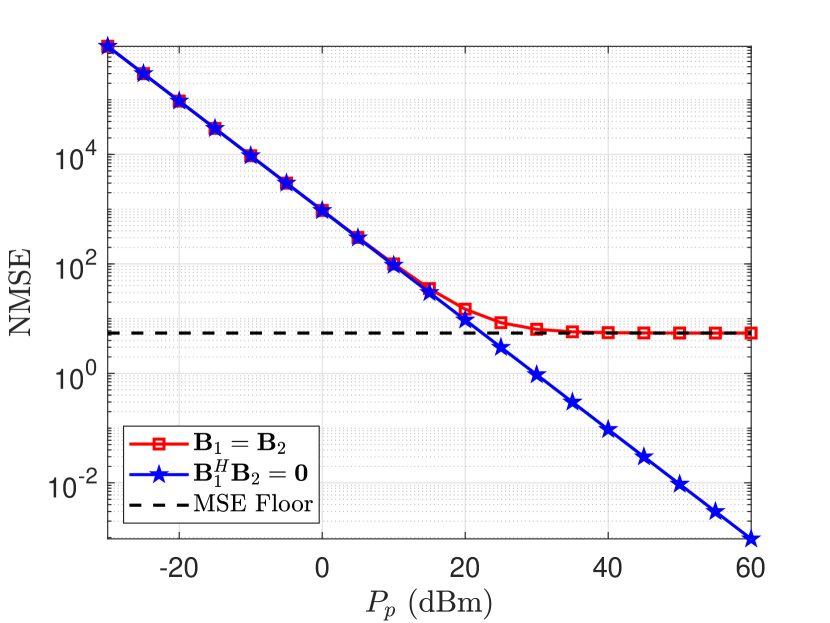
Figure 2: Pilot transmission power versus the channel estimation NMSE for deterministic channels. Since the prior distribution of the parameter vector is not considered in the non-random parameter estimation framework, it is highly likely to obtain NMSEs greater than $1$.

VII-B Data Estimation with Deterministic Channels

In Fig. 3, the data estimation MSE performance with the two RIS pilot configurations is analyzed when the channel estimation SNR is high as in Section IV-A. That is, (24) is plotted for $\mathbf{B}_{1}=\mathbf{B}_{2}$ and $\mathbf{B}_{1}^{H}\mathbf{B}_{2}=\boldsymbol{0}$. In addition, the case where all of the channels are perfectly known is plotted to serve as the golden standard, labeled as Perfect CSI. However, even when all the channels are perfectly known, each RIS is assumed to be optimized independently according to the subscribed UE’s CSI. Note that although the channel estimation SNR is high, $\mathbf{B}_{1}=\mathbf{B}_{2}$ yields biased estimates of $\mathbf{g}_{1}$ due to pilot contamination caused by self-interference. On the other hand, $\mathbf{B}_{1}^{H}\mathbf{B}_{2}=\boldsymbol{0}$ yields the true $\mathbf{g}_{1}$ as the estimate, however, since BS $1$ is unaware of the path through the second RIS, the data estimate is biased, hence, there is still a high data transmission SNR floor. At around $P_{d}=5$ dBm, $\mathbf{B}_{1}=\mathbf{B}_{2}$ starts to approach the high-SNR floor. On the other hand, $\mathbf{B}_{1}^{H}\mathbf{B}_{2}=\boldsymbol{0}$ does not suffer from the lack of awareness of the second RIS path until around $P_{d}=20$ dBm. Hence, Fig. 3 clearly shows the benefit of configuring the RIS pilot configurations sequences orthogonally.

Figure 3: Data transmission power versus the data estimation NMSE for deterministic channels with high channel estimation SNR.

VII-C Channel Estimation Based on Correlated Rayleigh Fading Priors

In Fig. 4, the channel estimation performance with the two RIS pilot configurations are analyzed for correlated Rayleigh fading channels. Fig. 4 is generated by computing the trace of the channel estimation error covariance matrix provided in (31) and normalizing it by the factor of $\text{tr}(\boldsymbol{\Sigma}_{\mathbf{g}_{k}})$ for different $P_{p}$ values and different spatial channel correlation matrices. The spatial channel correlation matrices are computed for isotropic scattering based on the different RIS element geometries according to [26, Prop. 1].

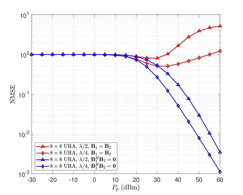
Figure 4: Pilot transmission power versus channel estimation MSE for different RIS geometries.

Note that configuring the RISs such that $\mathbf{B}_{1}=\mathbf{B}_{2}$ causes severe problems in channel estimation, that is, the MSE increases as pilot transmission power increases for all geometries while $\mathbf{B}_{1}^{H}\mathbf{B}_{2}=\boldsymbol{0}$ completely eliminates pilot contamination. In addition, one can note that as the spatial correlation increases, channel estimation performance also increases since different channel parameters contain more information from one another.

Furthermore, in Fig. 5, we demonstrate the two different components of the channel estimation error in the presence of inter-operator pilot contamination. While the red curve corresponds to the total NMSE and the blue curve corresponds to the NMSE in the absence of pilot contamination as usual, the green curve demonstrates the term coming from pilot contamination, as in (31). On the other hand, the black dashed line represents the asymptote of the channel estimation NMSE in the presence of pilot contamination, which is provided by (35). Note that as the transmission power increases, the NMSE coming from pilot contamination also increases up to a certain point, and converges to the trace of (35) for $\mathbf{B}_{1}=\mathbf{B}_{2}$ due to the fact that at very high transmission powers, the increase in pilot contamination cancels out with the increasing ability to estimating the channel.

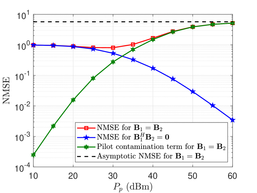
Figure 5: Different components of the channel estimation NMSE

VII-D Capacity Lower Bound for Reliable Communication Under Imperfect CSI

In Fig. 6, the capacity lower bound derived in Section VI is plotted against the data transmission power. This is performed by generating several channel realizations and computing (37). Note that when $\mathbf{B}_{1}=\mathbf{B}_{2}$, the capacity lower bound stops increasing after $P_{d}=30$ dBm while this happens at around $P_{d}=40$ dBm for $\mathbf{B}_{1}^{H}\mathbf{B}_{2}=\boldsymbol{0}$ when the effect of the misspecified channel during data transmission starts to appear. In any case, it is clear that configuring the RISs such that $\mathbf{B}_{1}^{H}\mathbf{B}_{2}=\boldsymbol{0}$ almost doubles the capacity lower bound.

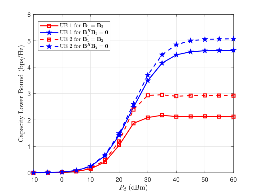
Figure 6: Data transmission power versus capacity lower bound for the two users.

VIII Conclusions

In this paper, we have studied the impact of pilot contamination in a system consisting of two wide-band RISs, two single-antenna UEs, and two co-located single-antenna BSs. We have demonstrated that the presence of multiple RISs in the same area causes pilot contamination, although the UEs are subscribed to different operators and transmit over disjoint narrow frequency bands. To combat this new type of pilot contamination, we have proposed the use of orthogonal RIS configurations during pilot transmission. For two different sets of assumptions, that is, deterministic and correlated Rayleigh-fading channel models, we have derived the channel and data estimation MSEs and the capacity lower bound in closed-form. In the numerical results, we have clearly shown that the proposed approach eliminates pilot contamination completely, and decreases data estimation MSE significantly for deterministic channels. On the other hand, we have also shown that the capacity lower bound almost doubles when the RISs are configured orthogonally during the pilot transmission step. While one might argue that this doubling comes at the expense of doubling the number of pilots, the estimates can be used for many data transmissions if the channel is static enough, resulting in a higher overall data rate. While this study covers the channel estimation performance in multi-operator RIS-based pilot contamination scenarios for both deterministic and stochastic channels, further analysis is needed for parametric channel models, which opens a new set of possibilities.

References

- [1] D. Gürgünoğlu, E. Björnson, and G. Fodor, “Impact of pilot contamination between operators with interfering reconfigurable intelligent surfaces,” 2023.
- [2] T. L. Marzetta, “Noncooperative cellular wireless with unlimited numbers of base station antennas,” IEEE Trans. Wireless Commun., vol. 9, no. 11, pp. 3590–3600, 2010.
- [3] L. Sanguinetti, E. Björnson, and J. Hoydis, “Toward Massive MIMO 2.0: Understanding spatial correlation, interference suppression, and pilot contamination,” IEEE Trans. Commun., vol. 68, no. 1, 2020.
- [4] J. Jose, A. Ashikhmin, T. L. Marzetta, and S. Vishwanath, “Pilot contamination and precoding in multi-cell TDD systems,” IEEE Trans. Wireless Commun., vol. 10, no. 8, pp. 2640–2651, 2011.
- [5] V. Saxena, G. Fodor, and E. Karipidis, “Mitigating pilot contamination by pilot reuse and power control schemes for massive MIMO systems,” in 2015 IEEE 81st Vehicular Technology Conference (VTC Spring), 2015, pp. 1–6.
- [6] G. Fodor, N. Rajatheva, W. Zirwas, L. Thiele, M. Kurras, K. Guo, A. Tolli, J. H. Sorensen, and E. De Carvalho, “An overview of massive MIMO technology components in METIS,” IEEE Communications Magazine, vol. 55, no. 6, pp. 155–161, 2017.
- [7] C. Pan, H. Ren, K. Wang, J. F. Kolb, M. Elkashlan, M. Chen, M. Di Renzo, Y. Hao, J. Wang, A. L. Swindlehurst, X. You, and L. Hanzo, “Reconfigurable intelligent surfaces for 6G systems: Principles, applications, and research directions,” IEEE Communications Magazine, vol. 59, no. 6, pp. 14–20, 2021.
- [8] E. Björnson, Ö. Özdogan, and E. G. Larsson, “Reconfigurable intelligent surfaces: Three myths and two critical questions,” IEEE Commun. Mag., no. 12, pp. 90–96, 2020.
- [9] G. T. de Araújo, A. L. F. de Almeida, R. Boyer, and G. Fodor, “Semi-blind joint channel and symbol estimation for IRS-assisted MIMO systems,” IEEE Transactions on Signal Processing, vol. 71, pp. 1184–1199, 2023.
- [10] R. Liu, M. Li, H. Luo, Q. Liu, and A. L. Swindlehurst, “Integrated sensing and communication with reconfigurable intelligent surfaces: Opportunities, applications, and future directions,” IEEE Wireless Communications, vol. 30, no. 1, pp. 50–57, 2023.
- [11] L. Wei, C. Huang, G. C. Alexandropoulos, C. Yuen, Z. Zhang, and M. Debbah, “Channel estimation for RIS-empowered multi-user MISO wireless communications,” IEEE Transactions on Communications, vol. 69, no. 6, pp. 4144–4157, 2021.
- [12] E. Björnson and P. Ramezani, “Maximum likelihood channel estimation for RIS-aided communications with LOS channels,” in Asilomar Conference on Signals, Systems and Computers, 2022.
- [13] C. Huang, A. Zappone, G. C. Alexandropoulos, M. Debbah, and C. Yuen, “Reconfigurable intelligent surfaces for energy efficiency in wireless communication,” IEEE Trans. Commun., vol. 18, no. 8, pp. 4157–4170, 2019.
- [14] Z. Zhang, L. Dai, X. Chen, C. Liu, F. Yang, R. Schober, and H. V. Poor, “Active RIS vs. passive RIS: Which will prevail in 6g?” IEEE Transactions on Communications, vol. 71, no. 3, pp. 1707–1725, 2023.
- [15] M. Rihan, A. Zappone, S. Buzzi, G. Fodor, and M. Debbah, “Passive vs. active reconfigurable intelligent surfaces for integrated sensing and communication: Challenges and opportunities,” IEEE Network, pp. 1–1, 2023.
- [16] N. Garg, H. Ge, and T. Ratnarajah, “Generalized superimposed training scheme in IRS-assisted cell-free massive mimo systems,” IEEE Journal of Selected Topics in Signal Processing, vol. 16, no. 5, pp. 1157–1171, 2022.
- [17] 3GPP, “NR; Physical channels and modulation,” 3rd Generation Partnership Project (3GPP), Technical Specification (TS) 38.211, 09 2022, version 17.4.0.
- [18] S. Zhang and R. Zhang, “Capacity characterization for intelligent reflecting surface aided MIMO communication,” IEEE Journal on Selected Areas in Communications, vol. 38, no. 8, pp. 1823–1838, 2020.
- [19] X. Pei, H. Yin, L. Tan, L. Cao, Z. Li, K. Wang, K. Zhang, and E. Björnson, “RIS-aided wireless communications: Prototyping, adaptive beamforming, and indoor/outdoor field trials,” pp. 8627–8640, 2021.
- [20] V. Tapio, A. Shojaeifard, I. Hemadeh, A. Mourad, and M. Juntti, “Reconfigurable intelligent surface for 5g NR uplink coverage enhancement,” in 2021 IEEE 94th Vehicular Technology Conference (VTC2021-Fall), 2021, pp. 1–5.
- [21] M. Vincenzi, A. Antonopoulos, E. Kartsakli, J. Vardakas, L. Alonso, and C. Verikoukis, “Cooperation incentives for multi-operator C-RAN energy efficient sharing,” in 2017 IEEE International Conference on Communications (ICC), 2017, pp. 1–6.
- [22] H.-T. Chien, Y.-D. Lin, H.-W. Chang, and C.-L. Lai, “Multi-operator fairness in transparent RAN sharing by soft-partition with blocking and dropping mechanism,” IEEE Transactions on Vehicular Technology, vol. 67, no. 12, pp. 11 597–11 605, 2018.
- [23] S. M. Kay, Fundamentals of Statistical Signal Processing, Volume I: Estimation Theory. Prentice Hall, 1993.
- [24] H. V. Poor, An Introduction to Signal Detection and Estimation (2nd Ed.). Berlin, Heidelberg: Springer-Verlag, 1994.
- [25] T. L. Marzetta, E. G. Larsson, H. Yang, and H. Q. Ngo, Fundamentals of Massive MIMO. Cambridge University Press, 2016.
- [26] E. Björnson and L. Sanguinetti, “Rayleigh fading modeling and channel hardening for reconfigurable intelligent surfaces,” IEEE Wireless Communications Letters, vol. 10, no. 4, pp. 830–834, 2021.