EHA: Entanglement-variational Hardware-efficient Ansatz for Eigensolvers

Abstract

Variational quantum eigensolvers (VQEs) are one of the most important and effective applications of quantum computing, especially in the current noisy intermediate-scale quantum (NISQ) era. There are mainly two ways for VQEs: problem-agnostic and problem-specific. For problem-agnostic methods, they often suffer from trainability issues. For problem-specific methods, their performance usually relies upon choices of initial reference states which are often hard to determine. In this paper, we propose an Entanglement-variational Hardware-efficient Ansatz (EHA), and numerically compare it with some widely used ansatzes by solving benchmark problems in quantum many-body systems and quantum chemistry. Our EHA is problem-agnostic and hardware-efficient, especially suitable for NISQ devices and having potential for wide applications. EHA can achieve a higher level of accuracy in finding ground states and their energies in most cases even compared with problem-specific methods. The performance of EHA is robust to choices of initial states and parameters initialization and it has the ability to quickly adjust the entanglement to the required amount, which is also the fundamental reason for its superiority.

I Introduction

Quantum computing has the potential to revolutionize many fields, including quantum many-body physics Huang et al. (2022); Stetcu et al. (2022); Morningstar et al. (2022), quantum chemistry McArdle et al. (2020); Elfving et al. (2021); Cao et al. (2022), material science Bauer et al. (2020); Ma et al. (2020); Bassman et al. (2021), and so on Egger et al. (2020); Cerezo et al. (2022). Among these, finding the ground state and its energy of Hamiltonians is a fundamental problem Huang et al. (2022); Stetcu et al. (2022); Morningstar et al. (2022); McArdle et al. (2020); Elfving et al. (2021). In the current noisy intermediate-scale quantum (NISQ) era Preskill (2018); Bharti et al. (2022, 2022), variational quantum eigensolvers (VQEs) Peruzzo et al. (2014); Cerezo et al. (2021); Tilly et al. (2022); Kattemölle and van Wezel (2022); Li et al. (2023) have been proposed to solve this problem with the hope that approximate solutions could be found for large systems which are intractable with classical computers.

VQEs work in a hybrid quantum-classical manner Callison and Chancellor (2022). They employ a parameterized quantum circuit (PQC) to generate parameterized trial states and the variational parameters are updated by a classical optimizer through minimizing the objective function, which in general is the expectation value of the Hamiltonian with respect to the trial state.

To enhance performance of VQEs, various methods have been developed from different perspectives. These include designing appropriate ansatzes for quantum circuits Ostaszewski et al. (2021a); Grimsley et al. (2019); Tang et al. (2021); Ostaszewski et al. (2021b); Du et al. (2022); Ding and Spector (2022); Grimsley et al. (2023), tailored initial states Quantum et al. (2020); Cade et al. (2020), proper parameter initializations Wang et al. (2023); Zhang et al. (2022a), developing efficient optimization methods Stokes et al. (2020), employing feedback for iterations Magann et al. (2022), and utilizing classical post-processing with neural networks Zhang et al. (2022b), among others Stair and Evangelista (2021); Cervera-Lierta et al. (2021); Fujii et al. (2022). It is clear that the ansatz of a quantum circuit directly determines the success of VQEs. For instance, if the quantum circuit is poorly expressible that cannot generate trial states close to the target state, then no other auxiliary methods can improve its performance Haug et al. (2021); Sim et al. (2019). There are mainly two ways to design ansatzes for quantum circuits: problem-agnostic and problem-specific Cerezo et al. (2021).

Hardware-efficient ansatz (HEA) is a well-known and widely used problem-agnostic method, which seeks to minimize the hardware noise by using native gates and connectives Kandala et al. (2017); Schuld et al. (2020); Choy and Wales (2023). When training quantum circuits based on HEAs, it often faces many challenges. Shallow HEA circuits are poorly expressible, and may cause the landscape of the cost function to be swamped with spurious local minima under global measurements Bittel and Kliesch (2021); Anschuetz and Kiani (2022). Deep circuits, however, will make the PQC too expressive resulting in barren plateaus (BPs) McClean et al. (2018); Holmes et al. (2022), i.e., the cost gradient is exponentially small with the number of qubits and/or the circuit depth. Both of these issues will make the PQC training extremely difficult. A major reason is that in most of existing HEAs, the entanglers are usually fixed, resulting in a lack of freedom to quickly adjust the entanglement of the trial states to the required amount. It is clear that the nature of the circuit ansatz determines the level of entanglement that can be achieved. On the one hand, generating a matched amount of entanglement is necessary to guarantee the convergency of eigensolvers based on HEAs. On the other hand, while entanglement can usually be quickly generated within a few layers, the excess entanglement cannot be removed efficiently Chen et al. (2022). It has been pointed out in Woitzik et al. (2020) that if the generated entanglement does not match the problem under study, it may hamper the convergence process. Moreover, it was argued in Marrero et al. (2021) that too much entanglement can result in BPs. In addition, it was stated in Leone et al. (2022) that even for shallow circuits, entanglement satisfying volume law should be avoided.

To address the training issues of PQCs, it has been suggested to design circuit ansatzes in a problem-specific manner. Examples include the Hamiltonian variational ansatz (HVA) also commonly referred to as a Trotterized adiabatic state preparation ansatz Wiersema et al. (2020), and the hardware symmetry preserving ansatz proposed in Lyu et al. (2023), which reduces the explored space of unitaries through symmetry preserving and is referred to as HSA in our paper. In quantum computational chemistry, some chemically inspired ansatzes have been proposed by adapting classical chemistry algorithms to run efficiently on quantum circuits McArdle et al. (2020). The most notable one is the unitary coupled cluster (UCC) Romero et al. (2018) adapted from the coupled cluster (CC) method Bartlett and Musiał (2007). The variational UCC method is able to converge when used with multi-reference initial states. The UCC is usually truncated at the single and double excitations, known as UCCSD Romero et al. (2018). In similar spirit to UCCSD, another commonly used ansatz has been proposed in Arrazola et al. (2022), which considers all single and double excitation gates acting on the reference state without flipping the spin of the excited particles, but where all gates are Givens rotations Arrazola et al. (2022). We refer to this ansatz as Givens rotation with all singles and doubles (GRSD) in this paper. Moreover, adaptive ansatzes have been presented in Grimsley et al. (2019); Tang et al. (2021), where the structure of quantum circuits are optimized adaptively. It has been shown that these adaptive ansatzes perform better in terms of both circuit depth and chemical accuracy than circuits that use parameters update alone. For these problem-specific methods, their performance usually relies upon choices of initial reference states Cai (2020); Skogh et al. (2023); Jattana et al. (2023), which are often hard to determine.

In this paper, we present a hardware-efficient ansatz for eigensolvers which allows for rapid adjustment of the entanglement to the required amount by making entanglers variational. Our ansatz is thus referred to as Entanglement-variational Hardware-efficient Ansatz (EHA). We validate its efficiency via numerical comparison with some widely used VQE ansatzes. By solving benchmark problems in quantum many-body physics and quantum chemistry, our EHA has the following advantages: 1) It is hardware-efficient and can be applied to various kinds of problems, particularly suitable for NISQ devices. 2) In most of numerical experiments, EHA can attain a higher level of accuracy than other ansatzes, even as compared with problem-specific ansatzes. 3) For different choices of initial reference states and variational parameters, the performance of EHA is more robust as compared to other ansatzes. 4) The variational entangler design enables EHA to quickly adjust the entanglement to the desired amount, which is also the fundamental reason for its superiority.

This paper is organized as follows. In Section II, for subsequent comparison, we first introduce several basic models and corresponding ansatzes. Then we present our EHA, and demonstrate its advantages via numerical comparisons with other ansatzes in Section III. Section IV concludes the paper. Since we utilize many abbreviations, for the convenience of reading, we summarize the frequently-used abbreviations and their full expressions in Table 1.

	Abbreviations	Descriptions
Quantum many-body model
	HM	Heisenberg Model
	TFIM	Transverse Field Ising Model
	BHM	Bose Hubbard Model
Variational Quantum Eigensolver(VQE) ansatz
	EHA	Entanglement-variational
		Hardware-efficient Ansatz
	HEA	Hardware-Efficient Ansatz
	HVA	Hamiltonian Variational Ansatz
	HSA	Hardware Symmetry preserving Ansatz
	GRSD	Givens Rotations with all
		Single and Double excitations
	UCCSD	Unitary Coupled Cluster with all
		Single and Double excitations
	ADAPT-VQE	Adaptive Derivative-Assembled
		Pseudo-Trotter ansatz-VQE

Table 1: Glossary.

II Preliminaries

In this paper, we focus on the task of finding ground eigenstates and their corresponding eigenenergies of Hamiltonians in quantum many-body physics and quantum chemistry. In this section, we introduce the models and ansatzes to be used for comparison with our EHA.

II.1 Quantum many-body models

For quantum many-body physics, we first consider a 1-dimensional chain Heisenberg model (HM) consisting of $N$ spins Wiersema et al. (2020); Lyu et al. (2023), whose Hamiltonian reads

$$H_{\mathrm{HM}}=J\sum_{i=1}^{N-1}(\sigma^{x}_{i}\sigma^{x}_{i+1}+\sigma^{y}_{i}\sigma^{y}_{i+1}+\sigma^{z}_{i}\sigma^{z}_{i+1}),$$ (1)

where $J=1$ sets the unit of energy, $\sigma^{x}_{i},~{}\sigma^{y}_{i}$ and $\sigma^{z}_{i}$ denote the Pauli $X$, $Y$ and $Z$ operators acting on the $i$-th qubit, respectively. The Hamiltonian Eq. (1) describes a model of interacting systems that cannot be mapped to free fermions. It supports symmetries including the conservation of the spin components in all directions, i.e. $[H_{\mathrm{HM}},S_{\alpha}]=0$ with $S_{\alpha}=\frac{1}{2}\sum_{i}\sigma_{i}^{\alpha}$ for $\alpha=x,~{}y$ and $z$, as well as the total spin, namely $[H_{\mathrm{HM}},S_{\mathrm{tot}}^{2}]=0$ with $S_{\mathrm{tot}}^{2}=S_{x}^{2}+S_{y}^{2}+S_{z}^{2}$.

We also consider free fermionic systems described by the transverse field Ising model (TFIM) Wiersema et al. (2020); Lyu et al. (2023), whose Hamiltonian reads

$$H_{\mathrm{TFIM}}=J_{z}\sum_{i=1}^{N-1}\sigma^{z}_{i}\sigma^{z}_{i+1}+h_{x}\sum_{i=1}^{N}\sigma^{x}_{i},$$ (2)

where $J_{z}$ represents the exchange coupling and $h_{x}$ depicts the strength of the transverse magnetic field. For this Hamiltonian, it is well-known that a quantum phase transition occurs at $J_{z}=h_{x}$, and at this critical point, the ground state is highly entangled and in a complex form Lyu et al. (2023).

II.2 Hardware-efficient ansatzes

In the NISQ era, VQEs have been proposed for eigensolvers with the hope to demonstrate potential quantum advantages when dealing with large systems which are beyond the power of classical computers.

Given a Hamiltonian $H$, when employing VQEs, we first need to design an ansatz to build a PQC $U(\boldsymbol{{\theta}})$ with variational parameters $\boldsymbol{\theta}$. Staring from a given initial reference state $|\psi_{0}\rangle$, we use the generated trial state $|\psi(\boldsymbol{{\theta}})\rangle=U(\boldsymbol{\theta})|\psi_{0}\rangle$ to approximate the ground state of $H$. The variational parameters $\boldsymbol{\theta}$ are adaptively updated by a classical optimizer via minimizing the expectation of $H$ at the trial state, which reads

$$C(\boldsymbol{\theta})=\operatorname{Tr}\left[HU(\boldsymbol{\theta})|\psi_{0}\rangle\langle\psi_{0}|U^{\dagger}(\boldsymbol{\theta})\right].$$ (3)

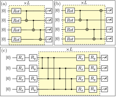
Figure 1: Quantum circuits for HEAs. (a) CX-line, whose single-qubit modules are $Rot$ gates defined in Eq. (4), and the entangling gates are CX gates arranged in a line pattern. (b) CX-ring, whose entangling gates are arranged in a ring pattern. (c) CZ-complete, whose single-qubit modules are $R_{y}R_{x}$ gates, and the entangling gates are CZ gates arranged in a complete pattern. The yellow shaded circuits are repeated for $L$ times.

To minimize the hardware noise in the NISQ era, HEAs have been widely used for eigensolvers. Three commonly used HEAs are illustrated in Fig. 1, and will be compared with our EHA. The initial reference state of these three HEAs is usually set to be $\rho_{0}=|0\rangle\langle 0|$. For the circuit in Fig. 1(a), the single-qubit rotations take the form of

$$Rot(\phi,\theta,\omega)=R_{z}(\omega)R_{y}(\theta)R_{z}(\phi),$$ (4)

with $R_{z}(\phi)=e^{-i\phi Z/2}$, $R_{y}(\theta)=e^{-i\theta Y/2}$, and the entangling gates are CX gates arranged in a line pattern Choy and Wales (2023). Thus, we refer to it as CX-line. The ansatz in Fig. 1(b) is named after CX-ring, since its single-qubit modules and entangling gates are the same as those in CX-line, except that the entangling gates are in a ring pattern Schuld et al. (2020). For the ansatz in Fig. 1(c), its single-qubit rotations are in the form of $R_{y}(\theta)R_{x}(\phi)$ with $R_{x}(\phi)=e^{-i\phi X/2}$ Zhang et al. (2022a). Since its entangling gates are CZ gates arranged in a complete pattern Kim et al. (2021), we call it CZ-complete.

II.3 Problem-specific ansatzes

The problem-agnostic HEAs often suffer from difficult training issues. In addition, HEAs do not preserve any symmetry in general. In this subsection, we briefly introduce two important problem-specific ansatzes: Hamiltonian variational ansatz (HVA) Wiersema et al. (2020) and hardware symmetry preserving ansatz (HSA) Lyu et al. (2023).

HVA: Assume the Hamiltonian $H$ can be decomposed into a summation with a total number of $S$ terms as

$$H=\sum_{s=1}^{S}H_{s}.$$ (5)

Then we can construct the HVA in the form of

$$U(\boldsymbol{\theta})=\prod_{l=1}^{L}\left[\prod_{s=1}^{S}\exp(-i\theta_{l,s}H_{s})\right].$$ (6)

Specifically, for an $N$-qubit HM described by Eq. (1), when the qubit number is even, its Hamiltonian can be decomposed into Wiersema et al. (2020)

$$H_{\mathrm{HM}}=H^{\text{even }}+H^{\text{odd }},$$

with

$$H^{\text{even }} =H_{xx}^{\text{even }}+H_{yy}^{\text{even }}+H_{zz}^{\text{even }},$$

$$H^{\text{odd }} =H_{xx}^{\text{odd }}+H_{yy}^{\text{odd }}+H_{zz}^{\text{odd }},$$

where for $\alpha=x,~{}y$ and $z$, $H_{\alpha\alpha}^{\mathrm{even}}=\sum_{i=1}^{N/2}\sigma_{2i-1}^{\alpha}\sigma_{2i}^{\alpha}$ and $H_{\alpha\alpha}^{\mathrm{odd}}=\sum_{i=1}^{N/2-1}\sigma_{2i}^{\alpha}\sigma_{2i+1}^{\alpha}.$ Then $U_{\mathrm{HM}}(\boldsymbol{\theta},\boldsymbol{\phi},\boldsymbol{\beta},\boldsymbol{\gamma})$ reads

$$U_{\mathrm{HM}}(\boldsymbol{\theta},\boldsymbol{\phi},\boldsymbol{\beta},\boldsymbol{\gamma})=\prod_{l=1}^{L}\Big{[}G\left(\theta_{l},H_{zz}^{\text{odd }}\right)G\left(\phi_{l},H_{xx}^{\text{odd }}\right)\cdot$$

$$G\left(\phi_{l},H_{yy}^{\text{odd }}\right)G\left(\beta_{l},H_{zz}^{\text{even }}\right)G\left(\gamma_{l},H_{xx}^{\text{even }}\right)G\left(\gamma_{l},H_{yy}^{\text{even }}\right)\Big{]},$$

with $G(x,A)=e^{-i\frac{x}{2}A}$.

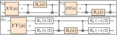
Figure 2: Hardware-efficient circuits for entangling gates. (a) Circuit for $XX$. (b) Circuit for $YY$. (c) Circuit for $ZZ$.

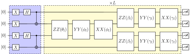
Figure 19: The HVA circuit for HM in Eq. (1). In HVA, the parameters of the entanglers are correlated.

The whole circuit for $U_{\mathrm{HM}}(\boldsymbol{\theta},\boldsymbol{\phi},\boldsymbol{\beta},\boldsymbol{\gamma})$ can be found in Fig. 19 in Appendix. To implement $U_{\mathrm{HM}}(\boldsymbol{\theta},\boldsymbol{\phi},\boldsymbol{\beta},\boldsymbol{\gamma})$, the entangling operators, $XX(\phi)=e^{-i\frac{\phi}{2}(X\otimes X)}$, $YY(\phi)=e^{-i\frac{\phi}{2}(Y\otimes Y)}$ and $ZZ(\phi)=e^{-i\frac{\phi}{2}(Z\otimes Z)}$, are employed whose circuits are illustrated in Fig. 2.

Note that the initial reference state plays a crucial role in problem-inspired ansatzes Quantum et al. (2020); Cade et al. (2020), which is quite different from the case in HEAs. To guarantee the efficiency of HVA for HM, the initial reference state is chosen to be ${\otimes^{\frac{N}{2}}}{|\Psi^{-}\rangle}$ with $|\Psi^{-}\rangle=\frac{1}{\sqrt{2}}(|01\rangle-|10\rangle)$.

As for an $N$-qubit TFIM with $J_{z}=h_{x}=-1$ and $N$ being even, the Hamiltonian $H_{\mathrm{TFIM}}$ can be decomposed into

$$H_{\mathrm{TFIM}}=-\sum_{i=1}^{N-1}\sigma^{z}_{i}\sigma^{z}_{i+1}-\sum_{i=1}^{N}\sigma^{x}_{i}=H_{zz}+H_{x},$$ (7)

with $H_{zz}=-\sum_{i}\sigma^{z}_{i}\sigma^{z}_{i+1}$ and $H_{x}=-\sum_{i}\sigma^{x}_{i}$. Then the HVA $U_{\mathrm{TFIM}}(\boldsymbol{\beta},\boldsymbol{\gamma})$ reads

$$U_{\mathrm{TFIM}}(\boldsymbol{\beta},\boldsymbol{\gamma})=\prod_{l=1}^{L}\left[\exp(-i\frac{\beta_{l}}{2}H_{zz})\exp(-i\frac{\gamma_{l}}{2}H_{x})\right],$$

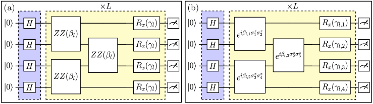
Figure 21: The HVA and HSA circuits for TFIM in Eq. (7). (a) The HVA circuit. In each block, there are only two variational parameters, one for the single qubit rotational gates and the other for the entanglers. (b) The HSA circuit. The gates have different parameters in general. The entangler $e^{i\beta\sigma^{z}_{1}\sigma^{z}_{2}}$ can be realized by setting $\theta=0$ and $\phi=0$ in Fig. 20(b).

whose circuit diagram is illustrated in Fig. 21(a) in Appendix. For TFIM, the initial reference state is chosen to be ${\otimes^{N}}{|+\rangle}$ with $|+\rangle=\frac{1}{\sqrt{2}}(|0\rangle+|1\rangle)$.

HSA: In Lyu et al. (2023), a HSA was proposed to improve the performance of eigensolvers by exploiting the symmetries of the Hamiltonian.

To be specific, if the ansatz $U(\boldsymbol{\theta})$ satisfies $[U(\boldsymbol{\theta}),S_{z}]=0$, then it conserves the number of excitation. While if $[U(\boldsymbol{\theta}),S_{\mathrm{tot}}^{2}]=0$, then it preserves the total spin. To realize HSA, the following more complex entangling gate Vatan and Williams (2004)

$$\mathcal{N}(\theta,\phi,\beta)=e^{i\left(\theta\sigma^{x}_{1}\sigma^{x}_{2}+\phi\sigma^{y}_{1}\sigma^{y}_{2}+\beta\sigma^{z}_{1}\sigma^{z}_{2}\right)}.$$

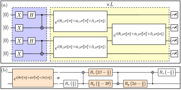
Figure 20: The HSA circuit for HM in Eq. (1). (a) The architecture of HSA. (b) Circuit for realizing the entangler $e^{i(\theta\sigma^{x}_{1}\sigma^{x}_{2}+\phi\sigma^{y}_{1}\sigma^{y}_{2}+\beta\sigma^{z}_{1}\sigma^{z}_{2})}$ used in HSA.

has been employed. The circuit of realizing $\mathcal{N}(\theta,\phi,\beta)$ is shown in Fig. 1(b) in Lyu et al. (2023) (Fig. 20(b) in Appendix).

As for the HM in Eq. (1), a single block circuit for realizing $S_{z}$-conserving and $S_{\mathrm{tot}}$-conserving ansatz is shown in Fig. 1(c) and Fig. 1(d) in Lyu et al. (2023), respectively. For ease of reading, we illustrate the HSA circuit in Fig. 20 in Appendix. Since the ground state of the Hamiltonian Eq. (1) is a global singlet with both the total spin $s=0$ and the spin component $s_{z}=0$, the initial reference state is chosen to be ${\otimes^{\frac{N}{2}}}{|\Psi^{-}\rangle}$ to guarantee the preservation of these symmetries in trial states.

The authors in Lyu et al. (2023) also generalized HSA to solve TFIM, whose circuit is shown in Fig. 7(a) in Lyu et al. (2023) (Fig. 21(b) in Appendix). The initial reference state is chosen to be ${\otimes^{N}}|+\rangle$.

II.4 Quantum chemistry models and ansatzes

Solving the low lying energies of the electrons in molecules has attracted significant attention McArdle et al. (2020) since it was first introduced by Aspuru-Guzik et al. (2005) in the context of quantum computational chemistry. It is often a starting point for more complex analysis in chemistry, including the calculation of reaction rates, the determination of molecular geometries and thermodynamic phases, among others Helgaker et al. (2012).

In this paper, we try to find the ground eigenstates and eigenenergies of the electronic Hamiltonian of $\mathrm{H}_{3}^{+}$ cation, $\mathrm{HF}$, $\mathrm{H}_{5}$, $\mathrm{BeH_{2}}$ and $\mathrm{LiH}$ molecules. For conciseness, we work in atomic units, where the length unit is 1 $\mathrm{\SIUnitSymbolAngstrom}$ (1 $$\mathrm{\SIUnitSymbolAngstrom}$=1\times 10^{-10}$ m), and the energy unit is 1 Hartree (1 Hartree = $27.211$ eV). We utilize the second quantized representation to simulate chemical systems on a quantum computer Babbush et al. (2016). To do this, we need to select a basis set, which is used to approximate the spin-orbitals of the investigated molecule. A suitably large basis set is crucial for obtaining accurate results. In this paper, we take the Slater type orbital-$3$ Gaussians (STO-$3$G) Helgaker et al. (2013) as the spin-orbital basis for second quantization. Then we utilize the occupation number basis to represent whether a spin-orbital is occupied. Next we can employ the Jordan-Wigner encoding Nielsen (2005) to map the second quantized fermionic Hamiltonian into a linear combination of Pauli strings, each of which is a product of single qubit Pauli operators. More details can be found in McArdle et al. (2020).

While it is important to understand the whole procedure of how to map electronic structure problems onto a quantum computer, every step from selecting a basis to producing an encoded qubit Hamiltonian can be carried out using a quantum computational chemistry package such as OpenFermion McClean et al. (2020) and PennyLane Bergholm et al. (2018). In this paper, we adopt PennyLane to implement UCCSD and GRSD.

III Main Results

In this section, we first present our hardware-efficient ansatz having variational entangling gates for eigensolvers. We then compare it with the introduced ansatzes by focusing on models introduced in Section II.

III.1 Entanglement-variational hardware-efficient ansatz

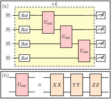
Figure 3: Quantum circuit for EHA. (a) The circuit consists of $L$ blocks, and each block is composed of a layer of single qubit rotational gates defined by Eq. (4) and variational entanglers $U_{\mathrm{ent}}$ arranged in a line pattern. (b) Each variational entangler $U_{\mathrm{ent}}$ is composed of $XX$, $YY$ and $ZZ$ gates in series, whose realizations are illustrated in Fig. 2. The variational parameters of the entanglers are (in general) different. The initial reference state is set to be $\otimes^{n}|0\rangle$.

Our aim is to design a hardware-efficient ansatz for eigensolvers which can be efficiently applied to solve various kinds of Hamiltonians for different systems.

To approximate target ground states, it is imperative to generate trial states having a matched amount of entanglement. However, there is a lack of freedom to adjust entanglement to the required level in most of existing HEAs, as their entanglers are fixed. The entanglement can usually be generated within a few layers, however, once the entanglement is in excess of requirement, it cannot be removed efficiently. The excess entanglement will result in too much expressibility leading to the phenomenon of BPs, which makes the training extremely difficult and greatly hampers the efficiency of HEAs.

Note that the entanglement is generated through entangling gates. Therefore, to improve the ability of regulating the generated entanglement of HEAs, a natural idea is to make entangling gates tunable with variational parameters. Based on this, we present our entanglement-variational hardware-efficient ansatz (EHA) as illustrated in Fig. 3.

It is clear that the entanglers

$$U_{\mathrm{ent}}(\boldsymbol{\theta_{l,i}})=ZZ(\theta_{l,i,3})YY(\theta_{l,i,2})XX(\theta_{l,i,1})$$

are tunable, which is the most significant difference from existing HEAs. Our ansatz is hardware-efficient, since the variational $XX$, $YY$ and $ZZ$ gates can be realized by native single qubit gates and CX gates as illustrated in Fig. 2. Moreover, we would like to point out that since the entanglers $XX$, $YY$ and $ZZ$ are native to hardwares themselves in some quantum computers Debnath et al. (2016), this can further significantly improve the efficiency of our EHA.

Although HVA and HSA also employ variational $XX$, $YY$ and $ZZ$ gates to implement entangling operations, the principle of their design is rather different from our EHA. There they first decompose the Hamiltonian of a specific problem into components as in Eq. (5), and then design variational circuits to realize each component Hamiltonian as described by Eq. (6). Note that in quantum many-body physics, Hamiltonians are described in terms of Pauli strings. Thus, when realizing the component Hamiltonians, variational gates, e.g., $XX$, naturally appear. Their constructed circuits are problem-specific. However, our EHA is problem-agnostic and can be applied to various problems.

In the following subsections, we compare our EHA with the ansatzes introduced in Section II in finding the ground state and its energy of Hamiltonians of various kinds of systems. In this paper, the actual ground state and its energy of Hamiltonians are obtained by employing the classical method NumPy Harris et al. (2020). We demonstrate that as compared with other ansatzes, our EHA can approximate the target ground states with a higher level of accuracy in most cases, and its performance is more robust with respect to different initializations and different initial states. In addition, our EHA can quickly adjust the entanglement of trial states to the required amount.

III.2 Higher level of accuracy and robustness

III.2.1 Quantum many-body problems

In the first part of Subsection III.2, we focus on finding eigenstates of a $12$-qubit HM in Eq. (1) and an 8-qubit TFIM in Eq. (2).

Since 2-qubit entangling gates are valuable resources in quantum computing, when comparing the performance of different ansatzes, to be fair, we ensure that they employ roughly the same number of basic 2-qubit entangling gates. As an illustration, when solving an $N$-qubit HM ($N$ is even), as shown in Fig. 2 and Fig. 3, our EHA utilizes a total number of $6(N-1)$ CX gates per block. While for each block, there are $(N-1)$ CX gates for CX-line, $N$ CX gates for CX-ring, $\frac{N(N-1)}{2}$ CZ gates for CZ-complete, $6(N-1)$ CX gates for HVA, and $3(N-1)$ CX gates for HSA. Here, we do not include the CX gates utilized to prepare the initial reference states for HVA and HSA. Thus, if there are $L$ blocks in our EHA, then the number of blocks should be $6L$ for CX-line, $\left\lceil\frac{6L(N-1)}{N}\right\rceil$ for CX-ring, $\left\lceil\frac{12L}{N}\right\rceil$ for CZ-complete, $L$ for HVA and $2L$ for HSA. Here, $\left\lceil\cdot\right\rceil$ denotes the roundup function.

As for the initialization of variational parameters, for CZ-complete, we use Gaussian initialization whose mean is 0 and variance is $1/L$ as mentioned in Zhang et al. (2022a). While for the other ansatzes, we adopt the uniform distribution $\mathcal{U}[-\pi,\pi]$. We employ the Adam optimizer provided by PennyLane for training, and the step size is set to be $0.01$ for all ansatzes, unless otherwise stated. Each ansatz is implemented $10$ times, and for each realization the initial parameters are drawn according to the assumed distribution. In the following figures, otherwise stated, the black dashed line denotes the actual ground state energy of the considered case, which serves as a baseline for comparison. All the other lines indicate the respective average value of the expectation of the considered Hamiltonian over $10$ realizations for different ansatzes. The shaded areas represent the smallest area that includes all the behaviors of the 10 realizations.

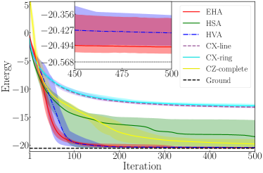
Figure 4: Comparison of our EHA with other ansatzes for HM in Eq. (8). The inset illustrates the fine difference between EHA and HVA. Our EHA is superior to other ansatzes in obtaining a lower energy, and its performance is robust with respect to different realizations.

To compare, we first consider a $12$-qubit HM, whose Hamiltonian reads

$$H_{\mathrm{HM}}=\sum_{i=1}^{N}(\sigma^{x}_{i}\sigma^{x}_{i+1}+\sigma^{y}_{i}\sigma^{y}_{i+1}+\sigma^{z}_{i}\sigma^{z}_{i+1}),$$ (8)

with $N=12$. The numbers of blocks in our EHA, CX-line, CX-ring, CZ-complete, HVA and HSA are 10, 60, 55, 10, 10 and 20, respectively. We illustrate their performance in Fig. 4. From the perspective of the average energy over different realizations, it is clear that our EHA clearly outperforms all the other ansatzes. Among them, the performances of CX-ring and CX-line are very poor. The performance of HSA has an obvious gap with our EHA. In addition, our EHA is robust to different parameter initializations, since all the 10 realizations approximately converge to the actual ground state energy. In contrast, the performance of HSA is very sensitive to parameter initializations.

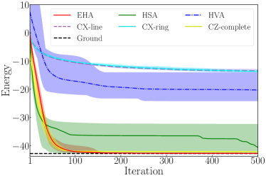
Figure 5: Comparison of our EHA with other ansatzes for the TFIM in Eq. (9). Our EHA is much better than all the other ansatzes, as it can robustly obtain a lower energy.

Next, for the $12$-qubit TFIM, we first consider a Hamiltonian which reads

$$H_{\mathrm{TFIM}}=-\sum_{i=1}^{N-1}\sigma^{z}_{i}\sigma^{z}_{i+1}+3.5\sum_{i=1}^{N}\sigma^{x}_{i},$$ (9)

with $N=12$. The numbers of blocks in our EHA, CX-line, CX-ring, CZ-complete, HVA, and HSA are 4, 24, 22, 4, 4 and 8, respectively. The results are illustrated in Fig. 5. We find that our EHA outperforms all the other ansatzes, as it can robustly attain a lower energy.

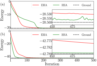
Figure 6: The best performance of EHA and HSA among 10 experiments for (a) HM in Eq. (8) and (b) TFIM in Eq. (9). The insets illustrate their fine differences. HSA is slightly better than our EHA in obtaining a lower energy.

Recall that HSA is a problem-specific ansatz that is utilized to improve the performance of VQE. However, from Fig. 4 and Fig. 5, it is clear that the sample variance of HSA is much larger than other ansatzes. This implies that its performance relies on different initial parameters. In fact, in the above experiments, it does not always provide a good approximation to the actual solution. However, under some initializations it does converge to the solution approximately. This is demonstrated in Fig. 6, where we plot the best performance of our EHA and HSA among 10 experiments for the HM in Eq. (8) and TFIM in Eq. (9). We find that from the perspective of the best performance, the problem-specific HSA is slightly better than our EHA. Nevertheless, it is important to note that our ansatz is problem-agnostic, and it is more robust to different realizations.

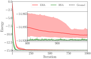
Figure 7: Comparison between our EHA and HSA for TFIM in Eq. (10). HSA outperforms EHA, as it attains a lower energy and converges faster.

We then consider the TFIM in Eq. (2) with $J_{z}=h_{x}=-1$, whose Hamiltonian reads

$$H_{\mathrm{TFIM}}=-\sum_{i=1}^{11}\sigma^{z}_{i}\sigma^{z}_{i+1}-\sum_{i=1}^{12}\sigma^{x}_{i}.$$ (10)

Recall that for the Hamiltonian Eq. (2), a quantum phase transition occurs at $J_{z}=h_{x}$, and at this critical point, the ground state is highly entangled and in a complex form Lyu et al. (2023). We compare our EHA and HSA, and demonstrate the experimental results in Fig. 7. We find that for TFIM in Eq. (10), HSA converges to the actual ground state energy closer and faster than our EHA. We will explain the reason behind this in Subsection III.3.

III.2.2 Quantum chemistry problems

Now we compare our EHA with chemically inspired ansatzes UCCSD and GRSD by focusing on the $\mathrm{HF}$ molecule and $\mathrm{H}_{3}^{+}$ cation. Since the quantum circuits for UCCSD and GRSD are much more complicated than our EHA, here we only focus on their performance. Recall that we adopt PennyLane to simulate UCCSD and GRSD (referred to as ALLSD in PennyLane). For all the three ansatzes, we start with the Hartree-Fock state Quantum et al. (2020), and project the state obtained from the corresponding ansatz to the feasible state space, which is spanned by the states considering all single and double excitations above the Hartree-Fock state. We show that our EHA is superior to both of them in robustly obtaining a lower energy.

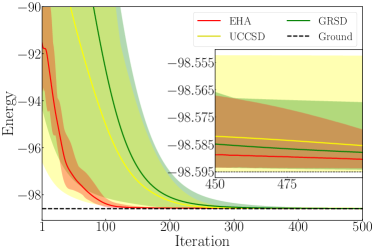
Figure 8: Comparison of our EHA with UCCSD and GRSD for $\mathrm{HF}$. The black dashed line denotes the ground energy of the $\mathrm{HF}$ Hamiltonian obtained by second quantization. Our EHA can robustly achieve a lower average energy as compared to UCCSD and GRSD.

As for the $\mathrm{HF}$ molecule, its bond length is set to be $1.1$. Our EHA consists of 12 qubits and has 18 blocks. We demonstrate the experimental results in Fig. 8. Here, the black dashed baseline denotes the ground energy of the $\mathrm{HF}$ Hamiltonian obtained by second quantization. We find that our EHA can achieve a lower energy on average and its performance is more robust with respect to different realizations as compared to UCCSD and GRSD. While for the best performance among 10 realizations, UCCSD and GRSD are slightly superior to our EHA.

As for the $\mathrm{H}_{3}^{+}$ cation, we need to modify the cost function Eq. (3) by adding a penalty term for our EHA. The reason is as follows. On the one hand the second quantization Hamiltonian of $\mathrm{H}_{3}^{+}$ depends only on the spin-orbital basis, and is independent of the number of electrons Helgaker et al. (2013). On the other hand, in contrast to UCCSD and GRSD, our EHA does not preserve particle numbers. Therefore, if there is no constraint, under EHA the trial states will converge to the ground state of $\mathrm{H}_{3}$ having 3 electrons, while $\mathrm{H}_{3}^{+}$ has only $2$ electrons. To address this issue, we can simply add a constraint on the number of electrons by means of penalty function. Specifically, we consider the cost function as

$$C(\theta)=\langle\psi(\theta)|H|\psi(\theta)\rangle+\beta[\langle\psi(\theta)|N|\psi(\theta)\rangle-2]^{2}.$$ (11)

Here, $H$ is the Hamiltonian of $\mathrm{H}_{3}^{+}$, $\beta$ is the penalty hyperparameter, and $N=\sum_{\alpha}\hat{c}_{\alpha}^{\dagger}\hat{c}_{\alpha}$ denotes the number operator with $\hat{c}^{\dagger}_{\alpha}$ and $\hat{c}_{\alpha}$ being the particle creation and annihilation operators, respectively, and the index $\alpha$ running over the basis of single-particle. Here, for $\mathrm{H}_{3}^{+}$, the bond length is set to be $1.1$. Our EHA consists of 6 qubits and has 9 blocks, and the hyperparameter $\beta=10$. The experimental results are shown in Fig. 9. We find that our EHA is much better than UCCSD and GRSD, as EHA can always achieve the ground energy for different realizations.

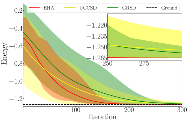
Figure 9: Comparison of our EHA with UCCSD and GRSD for $\mathrm{H}_{3}^{+}$. The black dashed line denotes the ground energy of the second quantization Hamiltonian of $\mathrm{H}_{3}^{+}$. Our EHA can always achieve the ground energy.

III.3 Ability to quickly adjust entanglment

Recall that to solve the ground state problem, it is imperative to generate a quantum state with the matched entanglement. In this subsection, we demonstrate that because of the variational entangler design in our EHA, it can rapidly adjust the entanglement to the required amount during the training process.

For an $N$-qubit system state $\rho$, denote by $\rho_{i}$ the state of the $i$-th qubit by taking partial trace over all the other qubits, namely, $\rho_{i}=\operatorname{Tr}_{\overline{i}}[\rho]$, where $\overline{i}$ denotes the subsystem excluding the $i$-th qubit. Here, we adopt the average von Neumann entropy

$$S\triangleq-\frac{1}{N}\sum_{i=1}^{N}\operatorname{Tr}\left[\rho_{i}\log(\rho_{i})\right]$$

to be the figure of merit for evaluating the entanglement of quantum state $\rho$.

For models already investigated in Subsection III.2, we now investigate their entanglement transitions of the generated trial states under different ansatzes during the optimization. In the following figures of this subsection, the black dashed line denotes the entanglement of the ground state, and the other lines denote the respective average value of the entanglement over 10 realizations under different ansatzes.

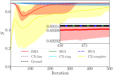
Figure 10: Entanglement transitions under different ansatzes for HM in Eq. (8). Our EHA can quickly adjust the entanglement to the desired amount.

For the $12$-qubit HM in Eq. (8), we illustrate the entanglement transitions (corresponding to Fig. 4) in Fig. 10. We find that the ground state has a large amount of entanglement. Under HVA and HSA, the entanglement of the generated quantum states stays at the same value as the desired amount during the optimization. This validates that for the problem-specific HVA and HSA, they only explore specific spaces of the unitaries during training. This is the main reason that HVA and HSA usually outperform problem-agnostic HEAs. However, as we mentioned and will be demonstrated in the next subsection, the performance of HVA and HSA depends heavily on the initial reference states, which are often hard to determine. For problem-agnostic HEAs, it is clear that our EHA can rapidly adjust the entanglement to the desired level, while other HEAs cannot. This is owing to the variational entangler design in our EHA.

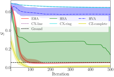
Figure 11: Entanglement transitions under different ansatzes for TFIM in Eq. (9). Our EHA is much better than other ansatzes in adjusting the entanglement to the required amount.

For the $12$-qubit TFIM in Eq. (9), we illustrate the entanglement transitions (corresponding to Fig. 5) in Fig. 11. We find that in this case the entanglement of the ground state is low. Under our EHA, the excess entanglement can be quickly removed and adjusted to the desired amount, which is hard to do with other ansatzes. The robustness of the entanglement transitions under different realizations is particularly poor for HSA.

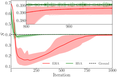
Figure 12: Entanglement transitions under HSA and EHA for TFIM in Eq. (10).

As for the TFIM in Eq. (10), we demonstrate the entanglement transitions under EHA and HSA in Fig. 12. From Fig. 7 and Fig. 12, we find that in this case HSA is superior to our EHA, as it can adjust the entanglement to the required level in a much quicker way. Recall that in the case where $J_{z}=h_{x}$, there is a quantum phase transition, and the ground state is highly entangled and in a complex form. This may make our EHA difficult to be trained, as it is based on variational entanglers. Nevertheless, our EHA can attain the ground state approximately, albeit at a slower rate.

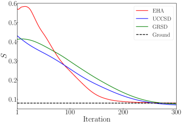
Figure 13: Entanglement transitions under EHA, UCCSD and GRSD for $\mathrm{H}_{3}^{+}$.

For the $\mathrm{H}_{3}^{+}$ cation, the entanglement transitions under EHA, UCCSD and GRSD (corresponding to Fig. 9) are shown in Fig. 13. Here, we only depict the average value of the entanglement over 10 realizations. We find that as compared with UCCSD and GRSD, EHA can quickly adjust the entanglement to the desired level.

III.4 The impact of initial reference states

In this subsection, we consider the impact of initial reference states on our EHA. Since the reference state in quantum chemistry problems is typically chosen as Hartree-Fock state, we only concern quantum many-body systems. Note that for the performed experiments, only HSA is slightly better than our EHA when considering the best performance of all realizations. We now demonstrate that the performance of our EHA is more robust with respect to different reference states as compared to HSA.

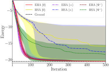
Figure 14: Comparison between our EHA and HSA under different initial reference states for HM in Eq. (8). The performance of our EHA is more robust than HSA.

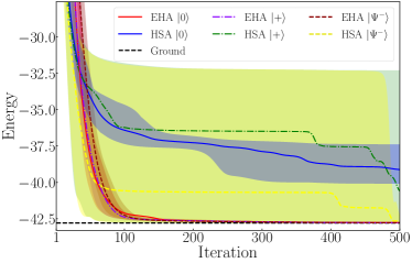
Figure 15: Comparison between our EHA and HSA under different initial reference states for TFIM in Eq. (9). The performance of our EHA is more robust than HSA.

Recall that for the HM in Eq. (8) and the TFIM in Eq. (9), the initial reference state of EHA is ${\otimes^{12}}|0\rangle$, while the reference states of HSA are ${\otimes^{6}}|\Psi^{-}\rangle$ and ${\otimes^{12}}|+\rangle$, respectively. Now we compare the performance of EHA and HSA under these three different reference states. We demonstrate the experimental results for HM and TFIM in Fig. 14 and Fig. 15, respectively. We find that for the HM, under the reference states ${\otimes^{12}}|+\rangle$ and ${\otimes^{12}}|0\rangle$, HSA cannot converge to the ground state. For the TFIM, while the performance of HSA becomes better if the the initial state is changed from the original ${\otimes^{12}}|+\rangle$ to ${\otimes^{6}}|\Psi^{-}\rangle$, HSA cannot converge to the ground state under the initial state ${\otimes^{12}}|0\rangle$. This validates that the performance of the problem-specific HSA is largely dependent on the reference state. In contrast to HSA, our problem-agnostic EHA can always perform well under different reference states, making it a strong candidate for quantum computing.

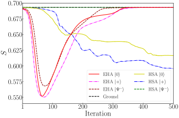
Figure 16: Entanglement transitions of EHA and HSA under different reference states for HM in Eq. (8). The black dashed line denotes the entanglement of the ground state. Other lines denote the respective average value of the entanglement over 10 realizations. The entanglement transitions of our EHA are much more robust than HSA under different initial states.

We can explain the above results by checking the corresponding entanglement transitions. As an illustration, we demonstrate the entanglement transitions of the HM (corresponding to Fig. 14) in Fig. 16. We find that once the initial state is changed to ${\otimes^{12}}|+\rangle$ or ${\otimes^{12}}|0\rangle$, HSA cannot maintain the same amount of entanglement as the ground state, and in turn resulting in poor performance.

III.5 Avoiding BP with reduced-domain initialization

In this subsection, we consider how to train our EHA with relatively large blocks.

As illustrated in Fig. 2 and Fig. 3, our EHA utilizes a total number of $6(N-1)$ CX gates per block. This makes the expressibility of EHA grow quickly as the number of blocks $L$ increases. However, it is well known that too expressive ansatz will result in the phenomenon of BP, making the training extremely difficult. Therefore, our EHA may suffer from BP when $L$ is large.

There have been many ways to mitigate the impact of BPs Sack et al. (2022); Friedrich and Maziero (2022); Mele et al. (2022); Wang et al. (2023); Zhang et al. (2022a). Here, we adopt the reduced-domain method introduced in Wang et al. (2023), where the domain of each initial parameter is properly reduced depending on the number of layers of the circuit. We demonstrate that this simple reduced-domain initialization Wang et al. (2023) can help train our EHA with relatively large blocks.

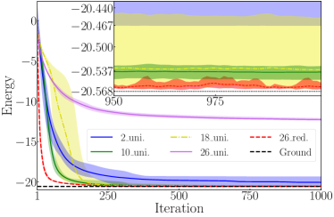
Figure 17: Performance of EHA under different numbers of blocks and initializations for HM in Eq. (8). With the reduced-domain initialization, the 26-block circuit can generate quantum states closer to the ground state in a faster way as compared to other schemes.

We focus on the $12$-qubit HM in Eq. (8), and consider four different numbers of blocks, namely, $L=2,10,18$ and $26$. The experimental settings are the same as those in Subsection III.2, except for the initialization.

We first draw the variational parameters according to the uniform distribution $\mathcal{U}[-\pi,\pi]$ as we have done in Subsection III.2. The numerical results are illustrated in Fig 17. We find that the $10$-block EHA has the best performance among the four considered cases, as it robustly converges to a lower energy. As compared with the 10-block EHA, the 2-block EHA is less expressible and cannot obtain better performance, while the 18-block EHA is more expressible but difficult to be trained Holmes et al. (2022), which is indicated by the slower convergence rate and larger sample variance. The 26-block EHA is too expressive to be trained. To address the training issue for large blocks of EHA, we leverage the reduced-domain initialization method Wang et al. (2023). Specifically, each variational parameter is drawn according to a reduced uniform distribution $\mathcal{U}[\frac{\pi}{2}-\frac{1}{\sqrt{L}},\frac{\pi}{2}+\frac{1}{\sqrt{L}}]$. In this case, the performance of the $26$-block EHA is plotted in Fig. 17. We find that with the reduced uniform initialization, the 26-block EHA has a much faster convergence rate, higher level of accuracy and robustness with respect to different realizations, as compared to other cases.

III.6 Performance Testing

In this subsection, we focus on the performance of our EHA on additional quantum chemistry and quantum many-body models.

We first compare our EHA with an ansatz termed adaptive derivative-assembled pseudo-Trotter ansatz variational quantum eigensolver (ADAPT-VQE), which was proposed in Grimsley et al. (2019) for molecular simulations. The key idea of ADAPT-VQE is to systematically grow the ansatz by adding fermionic operators one at a time to maximumly recover the correlation energy at each step. It has been shown that ADAPT-VQE outperforms UCC in terms of both circuit depth and chemical accuracy Grimsley et al. (2019). For all molecules, the ADAPT-VQE results are obtained by PennyLane, with the termination condition being gradient less than $10^{-3}$. While for our EHA, we find that for all experiments, the gradient is never below $10^{-3}$ before the end of training. This implies that the gradient of EHA is larger than ADAPT-VQE before the end of the optimization.

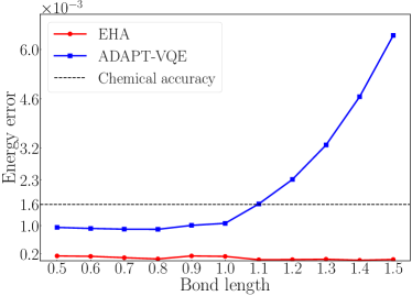
Figure 18: Ground energy error of EHA and ADAPT-VQE for $\mathrm{H}_{5}$. The energy error obtained by ADAPT-VQE exceeds the chemical accuracy and grows quickly when the bond length is larger than 1.1. While for our EHA, the energy error stays nearly at the same value as the bond length increases, and is about $1/8$ of the chemical accuracy.

Model	Qubits	Blocks	Ground energy	ADAPT-VQE energy	EHA-best	EHA-mean	EHA-STD
$\mathrm{BeH}_{2}$(1.1)	14	32	-15.5496	-15.5490	-15.5490	-15.5490	0.0000
LiH(1.11)	12	16	-7.8288	-7.8282	-7.8286	-7.8286	0.0000
HF(1.1)	12	18	-98.5951	-98.5942	-98.5948	-98.5947	0.0000

Table 2: Performance of EHA and ADAPT-VQE for different molecules.

Model	Blocks	Ground energy	Energy-best	Energy-mean	Energy-STD	Fidelity-best	Fidelity-mean	Fidelity-STD
HM(8)	14	-13.4997	-13.4994	-13.4993	0.0001	1.0000	1.0000	0.0000
HM(12)	28	-20.5684	-20.5679	-20.5675	0.0002	1.0000	0.9999	0.0000
HM(16)	42	-27.6469	-27.6461	-27.6459	0.0002	0.9999	0.9999	0.0000
TFIM(8)	6	-20.5018	-20.5018	-20.5015	0.0004	1.0000	1.0000	0.0000
TFIM(12)	6	-42.7890	-42.7889	-42.7880	0.0010	1.0000	1.0000	0.0000
TFIM(16)	8	-57.0763	-57.0760	-57.0759	0.0002	1.0000	1.0000	0.0000
BHM(8)	12	0.0000	0.0001	0.0002	0.0001	1.0000	1.0000	0.0000
BHM(16)	20	0.0000	0.0001	0.0002	0.0001	1.0000	1.0000	0.0000

Table 3: Performance of EHA for different quantum many-body systems.

We first consider solving the ground state of $\mathrm{H}_{5}$ at different bond lengths. Here, we consider the target ground state with $s_{z}=\frac{1}{2}$. Our EHA consists of $10$ qubits, $L=38$ blocks, and the initial parameters are drawn from a reduced uniform distribution $\mathcal{U}[\frac{\pi}{2}-\frac{1}{\sqrt{L}},\frac{\pi}{2}+\frac{1}{\sqrt{L}}]$. To guarantee the obtained state having $s_{z}=\frac{1}{2}$, similar to what we have done in dealing with $\mathrm{H}^{+}_{3}$, we add an $S_{z}$ penalty term (with the hyperparameter being 100) in the cost function in our EHA. We perform 2000 iterations, with the step size being 0.1 for the first 500 iterations, and 0.001 for the last 1500 iterations. We take the minimum energy during the training process as the approximate solution of the ground energy. We illustrate the ground energy error in Fig. 18. We find that when the bond length is larger than 1.1, the ground energy error obtained by ADAPT-VQE exceeds the chemical accuracy (1.6$\times$ $10^{-3}$) Eyring (1935) and grows quickly as the bond length increases. While for our EHA, the energy error remains nearly constant as the bond length increases, and is lower than ADAPT-VQE. Specifically, the ground energy error can maintain about $1/8$ of the chemical accuracy for bond length ranging from 0.5 to 1.5.

We now apply our EHA and ADAPT-VQE to other molecules. For our EHA we perform at most $3000$ iterations, and for different molecules the step size schedules are illustrated in Table 4 in Appendix. The results are demonstrated in Table 2. The first column lists the molecules with the bond length in parentheses, the second column shows the number of qubits needed after second quantization of the molecules, and the third column lists the blocks of our EHA. We also list the best value, mean value and the standard deviation (STD) of the energy obtained by our EHA in Table 2. It is clear that our EHA outperforms ADPT-VQE and has less than $5\times 10^{-5}$ standard deviation.

We further apply our EHA on other quantum many-body systems, where their corresponding step size schedules are illustrated in Table 4 in Appendix. We demonstrate the results in Table 3. The first column lists the models with the number of qubits in parentheses, where the HM and TFIM are described by Eq. (8) and Eq. (9), respectively. Here, the BHM denotes the Bose-Hubbard model (BHM) Fisher et al. (1989) in a chain lattice, whose Hamiltonian reads

$$H=-\left(\sum_{i=1}^{N-1}\hat{b}_{i}^{\dagger}\hat{b}_{i+1}+\text{h.c.}\right)+7\sum_{i=1}^{N}\hat{n}_{i}(\hat{n}_{i}-1),$$ (12)

where $\hat{b}_{i}^{\dagger}$ and $\hat{b}_{i}$ denote the Bosonic creation and annihilation operators on site $i$, respectively, and $\hat{n}_{i}=\hat{b}_{i}^{\dagger}\hat{b}_{i}$ denotes the number operator of site $i$. For BHM, we can use binary Bosonic mapping Huang et al. (2021) to transform the Hamiltonian in Eq. (12) into the form of a linear combination of Pauli strings, which is done by utilizing PennyLane in this paper. The number of blocks in our EHA is listed in the second column. In Table 3, we list the best value, mean value and the standard deviation of the energy and fidelity obtained by our EHA. We find that for all cases, our EHA can attain the ground energy with a very high level of accuracy. In the best case, the ground energy error is less than $1\times 10^{-3}$, and on average the ground energy error is less than the chemical accuracy of $1.6\times 10^{-3}$. Moreover, the standard deviation is very small, which is at most $1\times 10^{-3}$. The fidelity with the ground state is no smaller than $99.99\%$ on average, and the standard deviation is lower than $5\times 10^{-5}$.

IV Conclusion

In this paper, we propose an efficient hardware-efficient ansatz, EHA, for eigensolvers, in which the entanglers are designed to be variational rather than fixed. This entanglement-variational design allows the circuit to rapidly adjust the entanglement of the generated trial states to the required amount, and in turn greatly enhance the performance. We have demonstrated that our EHA can find approximate solutions for eigensolvers with a very high level of accuracy, and its performance is robust to choices of initial reference states and different realizations. We believe that our EHA is particularly suitable for NISQ era and will generate wide impact on developing algorithms with potential quantum advantages for various practical applications.

Appendix A APPENDIX

	Model	Step size	Iteration steps
	$\mathrm{BeH}_{2}$(1.1)	0.01	1000
		0.005	2000
	LiH(1.11)	0.01	1000
		0.005	1000
	HF(1.1)	0.01	1000
	HM(8)	0.01	1000
	HM(12)	0.005	1000
		0.001	1000
		0.0005	2000
	HM(16)	0.005	3000
		0.001	2000
		0.0005	2000
	TFIM(8)	0.01	2000
	TFIM(12)	0.01	4000
	TFIM(16)	0.01	4000
	BHM(8)	0.01	1000
	BHM(16)	0.01	500
		0.005	500

Table 4: The step size schedule for different models.

References

- Huang et al. (2022) Hsin-Yuan Huang, Richard Kueng, Giacomo Torlai, Victor V. Albert, and John Preskill, “Provably efficient machine learning for quantum many-body problems,” Science 377, eabk3333 (2022).
- Stetcu et al. (2022) I. Stetcu, A. Baroni, and J. Carlson, “Variational approaches to constructing the many-body nuclear ground state for quantum computing,” Phys. Rev. C 105, 064308 (2022).
- Morningstar et al. (2022) Alan Morningstar, Markus Hauru, Jackson Beall, Martin Ganahl, Adam G.M. Lewis, Vedika Khemani, and Guifre Vidal, “Simulation of quantum many-body dynamics with Tensor Processing Units: Floquet prethermalization,” PRX Quantum 3, 020331 (2022).
- McArdle et al. (2020) Sam McArdle, Suguru Endo, Alán Aspuru-Guzik, Simon C. Benjamin, and Xiao Yuan, “Quantum computational chemistry,” Rev. Mod. Phys. 92, 015003 (2020).
- Elfving et al. (2021) Vincent E. Elfving, Marta Millaruelo, José A. Gámez, and Christian Gogolin, “Simulating quantum chemistry in the seniority-zero space on qubit-based quantum computers,” Phys. Rev. A 103, 032605 (2021).
- Cao et al. (2022) Changsu Cao, Jiaqi Hu, Wengang Zhang, Xusheng Xu, Dechin Chen, Fan Yu, Jun Li, Han-Shi Hu, Dingshun Lv, and Man-Hong Yung, “Progress toward larger molecular simulation on a quantum computer: Simulating a system with up to 28 qubits accelerated by point-group symmetry,” Phys. Rev. A 105, 062452 (2022).
- Bauer et al. (2020) Bela Bauer, Sergey Bravyi, Mario Motta, and Garnet Kin-Lic Chan, “Quantum algorithms for quantum chemistry and quantum materials science,” Chem. Rev. 120, 12685–12717 (2020).
- Ma et al. (2020) He Ma, Marco Govoni, and Giulia Galli, “Quantum simulations of materials on near-term quantum computers,” npj Comput. Mater. 6, 85 (2020).
- Bassman et al. (2021) Lindsay Bassman, Miroslav Urbanek, Mekena Metcalf, Jonathan Carter, Alexander F. Kemper, and Wibe A. de Jong, “Simulating quantum materials with digital quantum computers,” Quantum Sci. Technol. 6, 043002 (2021).
- Egger et al. (2020) Daniel J. Egger, Claudio Gambella, Jakub Marecek, Scott McFaddin, Martin Mevissen, Rudy Raymond, Andrea Simonetto, Stefan Woerner, and Elena Yndurain, “Quantum computing for finance: State-of-the-art and future prospects,” IEEE Trans. Quantum Eng. 1, 3101724 (2020).
- Cerezo et al. (2022) M. Cerezo, Guillaume Verdon, Hsin-Yuan Huang, Lukasz Cincio, and Patrick J. Coles, “Challenges and opportunities in quantum machine learning,” Nat. Comput. Sci. 2, 567–576 (2022).
- Preskill (2018) John Preskill, “Quantum Computing in the NISQ era and beyond,” Quantum 2, 79 (2018).
- Bharti et al. (2022) Kishor Bharti et al., “Noisy intermediate-scale quantum algorithms,” Rev. Mod. Phys. 94, 015004 (2022).
- Peruzzo et al. (2014) Alberto Peruzzo, Jarrod McClean, Peter Shadbolt, Man-Hong Yung, Xiao-Qi Zhou, Peter J. Love, Alán Aspuru-Guzik, and Jeremy L. O’brien, “A variational eigenvalue solver on a photonic quantum processor,” Nat. Commun. 5, 4213 (2014).
- Cerezo et al. (2021) M. Cerezo et al., “Variational quantum algorithms,” Nat. Rev. Phys. 3, 625–644 (2021).
- Tilly et al. (2022) Jules Tilly et al., “The variational quantum eigensolver: a review of methods and best practices,” Phys. Rep. 986, 1–128 (2022).
- Kattemölle and van Wezel (2022) Joris Kattemölle and Jasper van Wezel, “Variational quantum eigensolver for the Heisenberg antiferromagnet on the kagome lattice,” Phys. Rev. B 106, 214429 (2022).
- Li et al. (2023) Andy C. Y. Li et al., “Benchmarking variational quantum eigensolvers for the square-octagon-lattice Kitaev model,” Phys. Rev. Res. 5, 033071 (2023).
- Callison and Chancellor (2022) Adam Callison and Nicholas Chancellor, “Hybrid quantum-classical algorithms in the noisy intermediate-scale quantum era and beyond,” Phys. Rev. A 106, 010101 (2022).
- Ostaszewski et al. (2021a) Mateusz Ostaszewski, Edward Grant, and Marcello Benedetti, “Structure optimization for parameterized quantum circuits,” Quantum 5, 391 (2021a).
- Grimsley et al. (2019) Harper R. Grimsley, Sophia E. Economou, Edwin Barnes, and Nicholas J. Mayhall, “An adaptive variational algorithm for exact molecular simulations on a quantum computer,” Nat. Commun. 10, 3007 (2019).
- Tang et al. (2021) Ho Lun Tang, V.O. Shkolnikov, George S. Barron, Harper R. Grimsley, Nicholas J. Mayhall, Edwin Barnes, and Sophia E. Economou, “qubit-ADAPT-VQE: An adaptive algorithm for constructing hardware-efficient ansätze on a quantum processor,” PRX Quantum 2, 020310 (2021).
- Ostaszewski et al. (2021b) Mateusz Ostaszewski, Lea M. Trenkwalder, Wojciech Masarczyk, Eleanor Scerri, and Vedran Dunjko, “Reinforcement learning for optimization of variational quantum circuit architectures,” Advances in Neural Information Processing Systems 34, 18182–18194 (2021b).
- Du et al. (2022) Yuxuan Du, Tao Huang, Shan You, Min-Hsiu Hsieh, and Dacheng Tao, “Quantum circuit architecture search for variational quantum algorithms,” npj Quantum Inf. 8, 62 (2022).
- Ding and Spector (2022) Li Ding and Lee Spector, “Evolutionary quantum architecture search for parametrized quantum circuits,” in Proceedings of the Genetic and Evolutionary Computation Conference Companion (2022) pp. 2190–2195.
- Grimsley et al. (2023) Harper R. Grimsley, George S. Barron, Edwin Barnes, Sophia E. Economou, and Nicholas J. Mayhall, “Adaptive, problem-tailored variational quantum eigensolver mitigates rough parameter landscapes and barren plateaus,” npj Quantum Inf. 9, 19 (2023).
- Quantum et al. (2020) Google AI Quantum, Collaborators*†, et al., “Hartree-Fock on a superconducting qubit quantum computer,” Science 369, 1084–1089 (2020).
- Cade et al. (2020) Chris Cade, Lana Mineh, Ashley Montanaro, and Stasja Stanisic, “Strategies for solving the Fermi-Hubbard model on near-term quantum computers,” Phys. Rev. B 102, 235122 (2020).
- Wang et al. (2023) Yabo Wang, Bo Qi, Chris Ferrie, and Daoyi Dong, “Trainability enhancement of parameterized quantum circuits via reduced-domain parameter initialization,” arXiv preprint arXiv:2302.06858 (2023).
- Zhang et al. (2022a) Kaining Zhang, Liu Liu, Min-Hsiu Hsieh, and Dacheng Tao, “Escaping from the barren plateau via gaussian initializations in deep variational quantum circuits,” Advances in Neural Information Processing Systems 35, 18612–18627 (2022a).
- Stokes et al. (2020) James Stokes, Josh Izaac, Nathan Killoran, and Giuseppe Carleo, “Quantum Natural Gradient,” Quantum 4, 269 (2020).
- Magann et al. (2022) Alicia B. Magann, Kenneth M. Rudinger, Matthew D. Grace, and Mohan Sarovar, “Feedback-based quantum optimization,” Phys. Rev. Lett. 129, 250502 (2022).
- Zhang et al. (2022b) Shi-Xin Zhang, Zhou-Quan Wan, Chee-Kong Lee, Chang-Yu Hsieh, Shengyu Zhang, and Hong Yao, “Variational quantum-neural hybrid eigensolver,” Phys. Rev. Lett. 128, 120502 (2022b).
- Stair and Evangelista (2021) Nicholas H. Stair and Francesco A. Evangelista, “Simulating many-body systems with a projective quantum eigensolver,” PRX Quantum 2, 030301 (2021).
- Cervera-Lierta et al. (2021) Alba Cervera-Lierta, Jakob S. Kottmann, and Alán Aspuru-Guzik, “Meta-variational quantum eigensolver: Learning energy profiles of parameterized Hamiltonians for quantum simulation,” PRX Quantum 2, 020329 (2021).
- Fujii et al. (2022) Keisuke Fujii, Kaoru Mizuta, Hiroshi Ueda, Kosuke Mitarai, Wataru Mizukami, and Yuya O. Nakagawa, “Deep variational quantum eigensolver: a divide-and-conquer method for solving a larger problem with smaller size quantum computers,” PRX Quantum 3, 010346 (2022).
- Haug et al. (2021) Tobias Haug, Kishor Bharti, and M. S. Kim, “Capacity and quantum geometry of parametrized quantum circuits,” PRX Quantum 2, 040309 (2021).
- Sim et al. (2019) Sukin Sim, Peter D. Johnson, and Alán Aspuru-Guzik, “Expressibility and entangling capability of parameterized quantum circuits for hybrid quantum-classical algorithms,” Adv. Quantum Technol. 2, 1900070 (2019).
- Kandala et al. (2017) Abhinav Kandala, Antonio Mezzacapo, Kristan Temme, Maika Takita, Markus Brink, Jerry M. Chow, and Jay M. Gambetta, “Hardware-efficient variational quantum eigensolver for small molecules and quantum magnets,” Nature 549, 242–246 (2017).
- Schuld et al. (2020) Maria Schuld, Alex Bocharov, Krysta M. Svore, and Nathan Wiebe, “Circuit-centric quantum classifiers,” Phys. Rev. A 101, 032308 (2020).
- Choy and Wales (2023) Boy Choy and David J. Wales, “Molecular energy landscapes of hardware-efficient ansatze in quantum computing,” J. Chem. Theory Comput. 19, 1197–1206 (2023).
- Bittel and Kliesch (2021) Lennart Bittel and Martin Kliesch, “Training variational quantum algorithms is NP-hard,” Phys. Rev. Lett. 127, 120502 (2021).
- Anschuetz and Kiani (2022) Eric R. Anschuetz and Bobak T. Kiani, “Quantum variational algorithms are swamped with traps,” Nat. Commun. 13, 7760 (2022).
- McClean et al. (2018) Jarrod R. McClean, Sergio Boixo, Vadim N. Smelyanskiy, Ryan Babbush, and Hartmut Neven, “Barren plateaus in quantum neural network training landscapes,” Nat. Commun. 9, 4812 (2018).
- Holmes et al. (2022) Zoë Holmes, Kunal Sharma, M. Cerezo, and Patrick J. Coles, “Connecting ansatz expressibility to gradient magnitudes and barren plateaus,” PRX Quantum 3, 010313 (2022).
- Chen et al. (2022) Yanzhu Chen, Linghua Zhu, Nicholas J. Mayhall, Edwin Barnes, and Sophia E. Economou, “How much entanglement do quantum optimization algorithms require?” in Quantum 2.0 (Optica Publishing Group, 2022) pp. QM4A–2.
- Woitzik et al. (2020) Andreas J. C. Woitzik, Panagiotis Kl. Barkoutsos, Filip Wudarski, Andreas Buchleitner, and Ivano Tavernelli, “Entanglement production and convergence properties of the variational quantum eigensolver,” Phys. Rev. A 102, 042402 (2020).
- Marrero et al. (2021) Carlos Ortiz Marrero, Mária Kieferová, and Nathan Wiebe, “Entanglement-induced barren plateaus,” PRX Quantum 2, 040316 (2021).
- Leone et al. (2022) Lorenzo Leone, Salvatore F. E. Oliviero, Lukasz Cincio, and M. Cerezo, “On the practical usefulness of the Hardware Efficient Ansatz,” arXiv preprint arXiv:2211.01477 (2022).
- Wiersema et al. (2020) Roeland Wiersema, Cunlu Zhou, Yvette de Sereville, Juan Felipe Carrasquilla, Yong Baek Kim, and Henry Yuen, “Exploring entanglement and optimization within the Hamiltonian Variational Ansatz,” PRX Quantum 1, 020319 (2020).
- Lyu et al. (2023) Chufan Lyu, Xusheng Xu, Man-Hong Yung, and Abolfazl Bayat, “Symmetry enhanced variational quantum spin eigensolver,” Quantum 7, 899 (2023).
- Romero et al. (2018) Jonathan Romero, Ryan Babbush, Jarrod R. McClean, Cornelius Hempel, Peter J. Love, and Alán Aspuru-Guzik, “Strategies for quantum computing molecular energies using the unitary coupled cluster ansatz,” Quantum Sci. Technol. 4, 014008 (2018).
- Bartlett and Musiał (2007) Rodney J. Bartlett and Monika Musiał, “Coupled-cluster theory in quantum chemistry,” Rev. Mod. Phys. 79, 291 (2007).
- Arrazola et al. (2022) Juan Miguel Arrazola, Olivia Di Matteo, Nicolás Quesada, Soran Jahangiri, Alain Delgado, and Nathan Killoran, “Universal quantum circuits for quantum chemistry,” Quantum 6, 742 (2022).
- Cai (2020) Zhenyu Cai, “Resource estimation for quantum variational simulations of the Hubbard model,” Phys. Rev. Appl. 14, 014059 (2020).
- Skogh et al. (2023) Mårten Skogh, Oskar Leinonen, Phalgun Lolur, and Martin Rahm, “Accelerating variational quantum eigensolver convergence using parameter transfer,” Electronic Structure 5, 035002 (2023).
- Jattana et al. (2023) Manpreet Singh Jattana, Fengping Jin, Hans De Raedt, and Kristel Michielsen, “Improved variational quantum eigensolver via quasidynamical evolution,” Phys. Rev. Appl. 19, 024047 (2023).
- Kim et al. (2021) Joonho Kim, Jaedeok Kim, and Dario Rosa, “Universal effectiveness of high-depth circuits in variational eigenproblems,” Phys. Rev. Res. 3, 023203 (2021).
- Vatan and Williams (2004) Farrokh Vatan and Colin Williams, “Optimal quantum circuits for general two-qubit gates,” Phys. Rev. A 69, 032315 (2004).
- Aspuru-Guzik et al. (2005) Alán Aspuru-Guzik, Anthony D. Dutoi, Peter J. Love, and Martin Head-Gordon, “Simulated quantum computation of molecular energies,” Science 309, 1704–1707 (2005).
- Helgaker et al. (2012) Trygve Helgaker, Sonia Coriani, Poul Jørgensen, Kasper Kristensen, Jeppe Olsen, and Kenneth Ruud, “Recent advances in wave function-based methods of molecular-property calculations,” Chem. Rev. 112, 543–631 (2012).
- Babbush et al. (2016) Ryan Babbush, Dominic W. Berry, Ian D. Kivlichan, Annie Y. Wei, Peter J. Love, and Alán Aspuru-Guzik, “Exponentially more precise quantum simulation of fermions in second quantization,” New J. Phys. 18, 033032 (2016).
- Helgaker et al. (2013) Trygve Helgaker, Poul Jorgensen, and Jeppe Olsen, Molecular electronic-structure theory (John Wiley and Sons, 2013).
- Nielsen (2005) Michael A. Nielsen, “The fermionic canonical commutation relations and the Jordan-Wigner transform,” School of Physical Sciences The University of Queensland 59 (2005).
- McClean et al. (2020) Jarrod R. McClean et al., “OpenFermion: the electronic structure package for quantum computers,” Quantum Sci. Technol. 5, 034014 (2020).
- Bergholm et al. (2018) Ville Bergholm et al., “PennyLane: Automatic differentiation of hybrid quantum-classical computations,” arXiv preprint arXiv:1811.04968 (2018).
- Debnath et al. (2016) S. Debnath, N. M. Linke, C. Figgatt, K. A. Landsman, K. Wright, and C. Monroe, “Demonstration of a small programmable quantum computer with atomic qubits,” Nature 536, 63–66 (2016).
- Harris et al. (2020) Charles R. Harris et al., “Array programming with NumPy,” Nature 585, 357–362 (2020).
- Sack et al. (2022) Stefan H. Sack, Raimel A. Medina, Alexios A. Michailidis, Richard Kueng, and Maksym Serbyn, “Avoiding barren plateaus using classical shadows,” PRX Quantum 3, 020365 (2022).
- Friedrich and Maziero (2022) Lucas Friedrich and Jonas Maziero, “Avoiding barren plateaus with classical deep neural networks,” Phys. Rev. A 106, 042433 (2022).
- Mele et al. (2022) Antonio A. Mele, Glen B. Mbeng, Giuseppe E. Santoro, Mario Collura, and Pietro Torta, “Avoiding barren plateaus via transferability of smooth solutions in a Hamiltonian Variational Ansatz,” Phys. Rev. A 106, L060401 (2022).
- Eyring (1935) Henry Eyring, “The activated complex in chemical reactions,” J. Chem. Phys. 3, 107–115 (1935).
- Fisher et al. (1989) Matthew P. A. Fisher, Peter B. Weichman, G. Grinstein, and Daniel S. Fisher, “Boson localization and the superfluid-insulator transition,” Phys. Rev. B 40, 546 (1989).
- Huang et al. (2021) Xin-Yu Huang, Lang Yu, Xu Lu, Yin Yang, De-Sheng Li, Chun-Wang Wu, Wei Wu, and Ping-Xing Chen, “Qubitization of Bosons,” arXiv preprint arXiv:2105.12563 (2021).