Polarization effects in elastic deuteron-electron scattering

Abstract

The differential cross section and polarization observables for the elastic reaction induced by deuteron scattering off electrons at rest are calculated in the one-photon-exchange (Born) approximation. Specific attention is given to the kinematical conditions, that is, to the specific range of incident energy and transferred momentum. The specific interest of this reaction is to access very small transferred momenta. Numerical estimates are given for polarization observables that describe the of single- and double-spin effects, provided that the polarization components (both, vector and tensor) of each particle in the reaction are determined in the rest frame of the electron target.

I Introduction

The use of the inverse kinematics in the experimental study of nuclear reactions has peculiar features. Inverse kinematics in hadron- electron reactions (where the projectile is much heavier than the target) is characterized by an extremely small momentum transfer squared. Therefore, these reactions induced by proton and deuteron beams as well, may be viewed as a possibility to measure the electromagnetic hadron form factors at very small momenta, inachieavable by direct kinematics.

Inverse kinematics was previously used in a number of the experiments to measure the pion or kaon radius in the elastic scattering of negative pions (kaons) from atomic electrons in a liquid-hydrogen target. The first experiment was done at Serpukhov Adylov et al. (1974) with pion beam energy of 50 GeV. Later, a few experiments were done at Fermilab with pion beam energy of 100 GeV Dally et al. (1977) and 250 GeV Dally et al. (1982). At this laboratory, the electromagnetic form factors of negative kaons were measured by direct scattering of 250 GeV kaons from stationary electrons Dally et al. (1980). Later on, a measurement of the pion electromagnetic form factor was done at the CERN SPS Amendolia et al. (1986, 1984) by measuring the interaction of 300 GeV pions with the electrons in a liquid hydrogen target.

The use of the inverse kinematics is proposed in a new experiment at CERN Abbiendi et al. (2016) to measure the running of the fine-structure constant in the space-like region by scattering high-energy muons (with energy 150 GeV) on atomic electrons, $\mu e\to\mu e$. The aim of the experiment is the extraction of the hadron vacuum polarization contribution.

In this work we consider the scattering of a polarized deuteron beam on a polarized electron target. We assume that the electron target is at rest and the deuteron beam interacts through the exchange of one photon with four momentum squared $-k^{2}=Q^{2}>0$. We follow the formalism from Ref. Gakh et al. (2011), which was developed for the process of the elastic proton-electron scattering $p+e^{-}\to p+e^{-}$.

Polarization observables are essential to disentangle the hadron structure and the reaction mechanism so to be able to test the validity and the predictions of hadron models . In particular, low-$Q^{2}$ data are used to determine the hadron charge radius, $r_{c}$. In case of protons, renewed interest in the charge radius is due to the discrepancy between several experiments, in atomic physics. Replacing an electron with a muon in an hydrogen atom is expected to give a more precise measurement on the proton radius, that enter as a correction in the Lamb shift of atomic levels, as the muonic atom is much more compact and therefore, corrective terms are more sensitive to the proton.

An experiment on muonic hydrogen Pohl et al. (2010) gives a value of $r_{c}=0.84184(67)$ fm. This value is one order of magnitude more precise but smaller by five standard deviation compared to the values of A1 Collaboration (Mainz) $(r_{c}=0.879(15))$ fm Bernauer et al. (2010) and CODATA $r_{c}=0.8768(69)$ fm $r_{c}=0.8768(69)$ fm Mohr et al. (2012). The problem of the charge proton radius puzzle stimulated new high precision PRad Gasparian (2014) and MUSE Cline et al. (2021) experiments to measure the $r_{c}$ in $e^{\pm}-p$ and $\mu^{\pm}-p$ scattering. In 2019 very unexpected result ($r_{c}=0.831$) of PRad experiment was published Xiong et al. (2019), that is even smaller the muonic hydrogen value. As concern the MUSE experiment, where the cross sections of the $e^{\pm}-p$ and $\mu^{\pm}-p$ scattering will be measured simultaneously, first results should appear soon, helping to solve the discrepancies between the Mainz and PRad results Cline et al. (2021). The reasons for these discrepancies have been searched in different effects, from new physics and high order radiative corrections to underestimated systematic effects, arising from the necessary extrapolation of the cross section data to $Q^{2}=0$. Note that the most recent CODATA evaluation takes into account the muonic hydrogen experiments, giving an updated vaue of $r_{c}=0.8414(19)$ fm Tiesinga et al. (2021).

An evaluation of the deuteron charge radius from electron-deuteron elastic scattering can be found in Ref. Sick and Trautmann (1998). The extracted value: $<r^{2}>=2.1230\pm 0.0033(stat)\pm 0.002(syst)$ fm is consistent with previous findings and with a calculation based on the present knowledge of nucleon-nucleon phase shifts. The corrections coming from the deuteron excited states in the intermediate state, the meson exchange currents, the six quark components are estimated to be less than a percent, in the region of low $Q^{2}$ values.

It is expected that the error associated to elastic electron scattering is larger than from atomic spectroscopy. The value deduced from laser spectroscopy $<r^{2}>=2.12718(13)_{exp}(89)_{th}$ can be found in Ref. Antognini et al. (2021) together with a review of light nuclei radii. It is in essential agreement with the CODATA recommended value for the deuteron rms squared radius is $<r^{2}>=2.12799(74)$ fm Tiesinga et al. (2021).

Any revision of the static (and dynamic) properties of the proton affects directly the description of light nuclei, in particular deuteron. At relatively large internal distances (small $Q^{2}$-values) the deuteron is considered to be a proton and a neutron, and small corrections would take into account effects beyond this simple picture.

One problem related to the extraction of the charge radius from form factor measurements is that it requires an extrapolation of the form factor for $Q^{2}\to 0$ (more precisely, of the form factor derivative) introducing an uncertainty. Systematic errors, as the choice of the fit function, may seriously affect the extraction of the radius Pacetti and Gustafsson (2016); Pacetti and Tomasi-Gustafsson (2020). Elastic hadron scattering by atomic electrons (which can be considered at rest) allows to access a range of very small transferred momenta, even for relatively large energies of the colliding particles.

Large interest in inverse kinematics (for the case of the elastic $p+e$ scattering) was arisen due to possible applications - the possibility to build beam polarimeters, for high energy polarized proton beams, in the RHIC energy range Glavanakov et al. (1996). The calculation of the spin correlation parameters, for the case of polarized proton beam and electron target, are sizeable and a polarimeter based on this reaction can measure the polarization of the proton beam Glavanakov et al. (1996). Numerical estimations of other polarization observables were done in Ref. Gakh et al. (2011). They showed that polarization effects may be sizable in the GeV range, and that the polarization transfer coefficients for $\vec{p}+e\rightarrow\vec{p}+e$ could be used to measure the polarization of high energy proton beams.

Recently inverse kinematics was used to investigate the nuclear reactions which can be hardly measured by other methods. In the paper Reifarth and Litvinov (2014) it was proposed to measure the neutron capture cross sections of unstable isotopes. To do so, the authors suggested a combination of a radioactive beam facility, an ion storage ring and a high flux reactor which allow a direct measurement of neutron induced reactions over a wide energy range on isotopes with half lives down to minutes. A direct measurement, in inverse kinematics, of the ${}^{17}O(\alpha,\gamma)^{21}Ne$ reaction has been performed at the DRAGON facility, at the TRIUMF laboratory, Canada Taggart et al. (2019). At this laboratory, the ${}^{22}Ne(p,\gamma)^{23}Na$ reaction has, for the first time, been investigated directly in inverse kinematics Williams et al. (2020). A total of 7 resonances were measured. The authors of the paper Phuc et al. (2019) analyze the (p, 2p) and (p, pn) reactions data measured, in inverse kinematics, at GSI (Darmstadt, Germany) for carbon, nitrogen and oxygen isotopes in the incident energy range of 300 – 450 MeV/n (see Holl et al. (2019) and references therein).

In this work, we calculate the differential cross section and polarization observables for the elastic deuteron-electron scattering in the one-photon-exchange approximation. Numerical estimations are given for various polarization observables. The possibility to build a polarimeter based on the elastic deuteron-electron scattering is also considered.

The paper is organized as follows. In Sec. II we give the details of the order of magnitude and the range which is accessible to the kinematic variables, as they are very specific for this reaction (Sec. II.A). The spin structure of the matrix element and the unpolarized cross section are derived and calculated in Sec. II.B in terms of deuteron form factors, the choice of which is discussed in Sec. II.C. Sec. III is devoted to the calculation of the polarization observables for the reaction $d+e\rightarrow d+e$. Analyzing powers in the $\vec{d}\,^{T}+e\to d+e$ reaction (when deuteron beam is tensor polarized) are calculated in Sec. III.A. The tensor polarization coefficients in the $d+e\to\vec{\vec{d}}^{T}+e$ reaction (when the scattered deuteron is tensor polarized) are given in Sec. III.B. The polarization transfer coefficients from a polarized target to the polarized recoil electron are calculated in Sec. III.C. In sections III.D - III.G we give the expressions for double polarization observables and derive various combinations the coefficients of the polarization correlation and polarization transfer between deuteron and electron, provided they have vector polarization. In Sec. III. H the vector polarization transfer from the initial deuteron to the scattered one is calculated. Sec. IV is devoted to discussion and conclusion.

II General formalism

Let us consider the reaction (Fig. 1)

$$d(p_{1})+e^{-}(k_{1})\to d(p_{2})+e^{-}(k_{2}),$$ (1)

where the particle momenta are indicated in parentheses, and $k=k_{1}-k_{2}=p_{2}-p_{1}$ is the four-momentum of the virtual photon. The reference system is the laboratory (Lab) system, where the electron target is at rest.

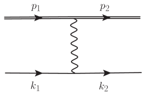
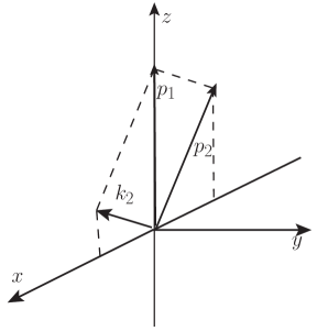
Figure 1: One photon exchange diagram of the process (1) and chosen coordinate axes in the rest frame of the initial electron.

A general characteristic of all reactions of elastic and inelastic hadron scattering by atomic electrons (which can be considered at rest) is the small value of the four momentum squared, even for relatively large energies of colliding hadrons. Let us first give details of the order of magnitude and the range which is accessible to the kinematic variables, as they are very specific for this reaction, and then derive the spin structure of the matrix element and the unpolarized and polarized observables.

II.1 Kinematics

In Lab system the four momentum transfer squared is a linear function of the scattered electron energy $\epsilon_{2}$

$$-k^{2}\equiv Q^{2}=-(k_{1}-k_{2})^{2}=2m(\epsilon_{2}-m),$$ (2)

where $m$ is the electron mass. The conservation of the four-momentum in the reaction (1) leads to the following relation between the energy $\epsilon_{2}$ and the scattering angle $\theta_{e}$ of the final electron:

$$\cos\theta_{e}=\displaystyle\frac{(E+m)(\epsilon_{2}-m)}{p\,\sqrt{\epsilon_{2}^{2}-m^{2}}},$$ (3)

where E is the deuteron beam energy, $p=\sqrt{E^{2}-M^{2}}$ is its modulus of the 3-momentum ($M$ is the deuteron mass). From Eq. 3 on can see that always $\cos\theta_{e}\geq 0$ (because $\epsilon_{2}>m$), and the electron can never scatter backward. The following relations hold:

$$\epsilon_{2}=m\frac{(E+m)^{2}+(E^{2}-M^{2})\cos^{2}\theta_{e}}{(E+m)^{2}-(E^{2}-M^{2})\cos^{2}\theta_{e}},\ \ Q^{2}=\frac{4m^{2}p^{2}\cos^{2}\theta_{e}}{(E+m)^{2}-p^{2}\cos^{2}\theta_{e}},$$ (4)

which show that the maximum energy of the final electron is achieved for forward scattering $(\cos{\theta_{e}}=1)$:

$$\epsilon_{2max}=m\frac{2E(E+m)+m^{2}-M^{2}}{M^{2}+2mE+m^{2}}.$$ (5)

From the expression for the $\epsilon_{2max}$, one can obtain the maximum value of the momentum transfer squared

$$Q^{2}_{max}=\frac{4m^{2}\,p^{2}}{M^{2}+2mE+m^{2}}.$$ (6)

One can see from Eqs.  (5, 6) that in the inverse kinematics, the available kinematical regions are reduced to small values of $\epsilon_{2}$ and $Q^{2},$ (compared with $E$ and $E^{2}$) which are proportional to $m$ and $m^{2},$ respectively. For example, at $E=10$ GeV one has $\epsilon_{2}\leq 25$ MeV and $Q^{2}\leq 25$ MeV${}^{2}.$ The upper limits of these quantities increase approximately as $E^{2}.$

As in the proton case, for one deuteron angle there may be two values of the deuteron energy, (and two corresponding values for the recoil- electron energy and angle, and for the transfer momentum squared $k^{2}$). This is a typical situation when the center of mass velocity is larger than the velocity of the projectile in the center of mass (c.m.), where all the angles are allowed for the recoil electron. From momentum conservation, on can find the following relation between the energy and the angle of the scattered deuteron $E_{2}$ and $\theta_{d}$:

$$E_{2}^{\pm}=\frac{(E+m)(M^{2}+mE)\pm p^{2}\cos\theta_{d}\sqrt{m^{2}-M^{2}\sin^{2}\theta_{d}}}{(E+m)^{2}-p^{2}\cos^{2}\theta_{d}}.$$ (7)

The two solutions coincide when the angle between the initial and final hadron takes its maximum value, which is determined by the ratio of the electron and scattered hadron masses, $\sin\theta_{d,max}=m/M$. Nevertheless, at fixed values of $\epsilon_{2}$ or $Q^{2}$, the energy of the scattered deuteron is unambiguous

$$E_{2}=E+m-\epsilon_{2}=E-\frac{Q^{2}}{2m}.$$ (8)

Hadrons are scattered from atomic electrons at very small angles, and the larger is the hadron mass, the smaller is the available angular range for the scattered hadron.

II.2 Unpolarized cross section

In the one-photon-exchange approximation, the matrix element ${\cal M}$ of reaction (1) can be written as:

$${\cal M}=\frac{e^{2}}{k^{2}}j^{\mu}J_{\mu},$$ (9)

where $j_{\mu}(J_{\mu})$ is the leptonic (hadronic) electromagnetic current. The leptonic current is

$$j_{\mu}=\bar{u}(k_{2})\gamma_{\mu}u(k_{1}),$$ (10)

where $u(k_{1,\,2})$ is the bispinor of the incoming (outgoing) electron. Following the requirements of Lorentz invariance, current conservation, parity and time-reversal invariance of the hadronic electromagnetic interaction, the general form of the electromagnetic current for the deuteron (which is a spin-one particle) is fully described by three form factors. The hadronic electromagnetic current can be written as A.I. and Rekalo (1977):

$$J_{\mu}=(p_{1}+p_{2})_{\mu}\left[-G_{1}(Q^{2})U_{1}\cdot U_{2}^{*}+\frac{1}{M^{2}}G_{3}(Q^{2})\left(U_{1}\cdot kU_{2}^{*}\cdot k+\frac{Q^{2}}{2}U_{1}\cdot U_{2}^{*}\right)\right]+$$ (11)

$$+G_{2}(Q^{2})\left(U_{1\mu}U_{2}^{*}\cdot k-U_{2\mu}^{*}U_{1}\cdot k\right),$$

where $U_{1\mu}$ and $U_{2\mu}$ are the polarization four vectors for the initial and final deuteron states. The functions $G_{i}(k^{2})$, i=1, 2, 3, are the deuteron electromagnetic form factors, depending only on the virtual photon four momentum squared. Due to the current hermiticity, these form factors are real functions in the region of space-like momentum transfer.

These form factors are related to the standard deuteron form factors: $G_{C}$ (charge monopole) $G_{M}$ (magnetic dipole) and $G_{Q}$ (charge quadrupole) by the following relations:

$$G_{M}(Q^{2})=-G_{2}(Q^{2}),\ \ G_{Q}(Q^{2})=G_{1}(Q^{2})+G_{2}(Q^{2})+2G_{3}(Q^{2}),$$ (12)

$$G_{C}(Q^{2})=\frac{2}{3}\tau\left[G_{2}(Q^{2})-G_{3}(Q^{2})\right]+\left(1+\frac{2}{3}\tau\right)G_{1}(Q^{2}),~{}\ \tau=\frac{Q^{2}}{4M^{2}}.$$

The standard form factors have the following normalization:

$$G_{C}(0)=1,\ \ G_{M}(0)=\frac{M}{m_{N}}\mu_{d},\ \ G_{Q}(0)=M^{2}{\hat{Q}}_{d},$$ (13)

where $m_{N}$ is the nucleon mass, $\mu_{d}=0.857$, Mohr and Taylor (2000), $\hat{Q}_{d}=0.2857$ fm² Ericson and Rosa-Clot (1983)) is the deuteron magnetic (quadrupole) moment.

Note also that

$$G_{1}(Q^{2})=\frac{1}{1+\tau}\Big{[}\tau G_{M}(Q^{2})+G_{C}(Q^{2})+\frac{\tau}{3}G_{Q}(Q^{2})\Big{]},$$

$$G_{3}(Q^{2})=\frac{1}{2(1+\tau)}\Big{[}G_{M}(Q^{2})-G_{C}(Q^{2})+\Big{(}1+\frac{2\tau}{3}\Big{)}G_{Q}(Q^{2})\Big{]}.$$

The matrix element squared is:

$$|{\cal M}|^{2}=16\pi^{2}\frac{\alpha^{2}}{Q^{4}}L^{\mu\nu}H_{\mu\nu},$$ (14)

where $\alpha=e^{2}/4\pi=1/137$ is the electromagnetic fine structure constant. The leptonic $L_{\mu\nu}$ and hadronic $H_{\mu\nu}$ tensors are defined as

$$L^{\mu\nu}=j^{\mu}j^{\nu*},~{}H_{\mu\nu}=J_{\mu}J_{\nu}^{*}.$$ (15)

The leptonic tensor, $L_{\mu\nu}^{(0)}$, for unpolarized initial and final electrons (averaging over the initial electron spin), has the form:

$$L_{\mu\nu}^{(0)}=-Q^{2}g_{\mu\nu}+2(k_{1\mu}k_{2\nu}+k_{1\nu}k_{2\mu}).$$ (16)

The contribution to the lepton tensor corresponding to the+ polarized electron target is

$$L_{\mu\nu}^{(p)}(s_{1})=2im\epsilon_{\mu\nu\rho\sigma}k^{\rho}s_{1}^{\sigma},\epsilon_{0123}=-1,$$ (17)

where $s_{1\sigma}$ is the initial electron polarization four-vector which satisfies following conditions: $k_{1}\cdot s_{1}=0,\,s_{1}^{2}=-1$.

The hadronic tensor $H_{\mu\nu}$ is calculated in terms of the deuteron electromagnetic form factors, using the explicit form of the electromagnetic current (11). The spin density matrices of the initial and final deuterons have the the following expressions :

$$\rho_{\alpha\beta}^{(i)}=-\frac{1}{3}\left(g_{\alpha\beta}-\frac{1}{M^{2}}p_{1\alpha}p_{1\beta}\right)+\frac{i}{2M}<\alpha\beta\eta_{1}p_{1}>+{\cal Q}_{\alpha\beta}^{(i)},$$ (18)

$$\rho_{\alpha\beta}^{(f)}=-\left(g_{\alpha\beta}-\frac{1}{M^{2}}p_{2\alpha}p_{2\beta}\right)+\frac{i}{2M}<\alpha\beta\eta_{2}p_{2}>+{\cal Q}_{\alpha\beta}^{(f)},$$

with the notation $<\alpha\beta ab>=\epsilon_{\alpha\beta\rho\sigma}a^{\rho}b^{\sigma}$. Here $\eta_{1\alpha}\,(\eta_{2\alpha})$ and ${\cal Q}_{\alpha\beta}^{(i)}\,({\cal Q}_{\alpha\beta}^{(f)})$ are the four vectors and tensors describing the vector and tensor (quadrupole) polarization of the initial (final) deuteron, respectively. The four-vector of the vector polarization of the initial (final) deuteron satisfies the following conditions: $\eta_{1}^{2}=-$1, $\eta_{1}\cdot p_{1}=0$ ($\eta_{2}^{2}=-$1, $\eta_{2}\cdot p_{2}=0$). The tensor ${\cal Q}_{\alpha\beta}^{(i)}$ satisfies the conditions ${\cal Q}_{\alpha\beta}^{(i)}\,g^{\alpha\beta}=0,$ $Q_{\alpha\beta}^{(i)}={\cal Q}_{\beta\alpha}^{(i)},$ ${\cal Q}_{\alpha\beta}^{(i)}\,p_{1}^{\alpha}=0$. The tensor ${\cal Q}_{\alpha\beta}^{(f)}$ satisfies the same conditions, after substitution: $i\to f$ and $p_{1}^{\alpha}\to p_{2}^{\alpha}$.

The hadronic tensor $H_{\mu\nu}(0)$, corresponding to the case of unpolarized initial and final deuterons can be written in the standard form in terms of two spin-independent structure functions:

$$H_{\mu\nu}(0)=H_{1}(Q^{2})\tilde{g}_{\mu\nu}+\frac{1}{M^{2}}H_{2}(Q^{2})P_{\mu}P_{\nu},$$ (19)

where $\tilde{g}_{\mu\nu}=g_{\mu\nu}-({k_{\mu}k_{\nu}})/{k^{2}}$, $P_{\mu}=(p_{1}+p_{2})_{\mu}$. Averaging over the spin of the initial deuteron, the structure functions $H_{i}(Q^{2})$, $i=1,2,$ can be expressed in terms of the electromagnetic form factors as:

$$H_{1}(Q^{2})=-\frac{2}{3}Q^{2}(1+\tau)G_{M}^{2}(Q^{2}),$$ (20)

$$H_{2}(Q^{2})=M^{2}\left[G_{C}^{2}(Q^{2})+\frac{2}{3}\tau G_{M}^{2}(Q^{2})+\frac{8}{9}\tau^{2}G_{Q}(Q^{2})\right].$$

The differential cross section is related to the matrix element squared (14) by

$$d\sigma=\displaystyle\frac{(2\pi)^{4}\overline{\left|{\cal M}\right|^{2}}}{4\sqrt{(k_{1}\cdot p_{1})^{2}-m^{2}M^{2}}}\displaystyle\frac{d^{3}\vec{k}_{2}}{(2\pi)^{3}2\epsilon_{2}}\displaystyle\frac{d^{3}\vec{p}_{2}}{(2\pi)^{3}2E_{2}}\delta^{4}(k_{1}+p_{1}-k_{2}-p_{2}),$$ (21)

$$\overline{\left|{\cal M}\right|^{2}}=16\pi^{2}\frac{\alpha^{2}}{Q^{4}}\,L^{\mu\nu}(0)\,H_{\mu\nu}(0),$$

where $\vec{p}_{2}\,(E_{2})$ is the 3-momentum (energy) of the scattered deuteron.

From this point on, the formalism differs from elastic electron-deuteron scattering, because we introduce a reference system where the electron is at rest. In this system, the differential cross section is written as

$$\frac{d\sigma}{d\epsilon_{2}}=\frac{1}{32\pi}\frac{\overline{\left|{\cal M}\right|^{2}}}{m\,p^{2}}.$$ (22)

The average over the spins of the initial particles has been included in the leptonic and hadronic tensors. Using Eq. (2) one can write

$$\frac{d\,\sigma}{d\,Q^{2}}=\frac{1}{64\pi}\frac{\overline{\left|{\cal M}\right|^{2}}}{m^{2}\,p^{2}}.$$ (23)

The differential cross section over the electron solid angle can be written as:

$$\frac{d\sigma}{d\Omega_{e}}=\frac{1}{32\pi^{2}}\,\frac{1}{m\,p}\,\frac{|\vec{k}_{2}|^{3}}{Q^{2}}\frac{\overline{\left|{\cal M}\right|^{2}}}{E+m},$$ (24)

where $d\,\Omega_{e}=2\pi\,d\cos\theta$ (due to the azimuthal symmetry) and we used the relation

$$d\epsilon_{2}=\displaystyle\frac{p}{E+m}\displaystyle\frac{|\vec{k}_{2}|^{3}}{m(\epsilon_{2}-m)}\displaystyle\frac{d\Omega_{e}}{2\pi}.$$ (25)

The differential cross section for unpolarized deuteron-electron scattering (23), in the coordinate system where the electron is at rest, can be written as:

$$\frac{d\sigma}{dQ^{2}}=\frac{\pi\,\alpha^{2}}{2\,m^{2}\,p^{2}}\frac{\cal D}{Q^{4}},\ \ {\cal D}=\frac{1}{2}\,L^{\mu\nu}(0)\,H_{\mu\nu}(0),$$ (26)

with

$${\cal D}=(-Q^{2}+2m^{2})H_{1}(Q^{2})+2\left[-Q^{2}M^{2}+2mE\left(2mE-Q^{2}\right)\right]\frac{H_{2}(Q^{2})}{M^{2}}.$$ (27)

The factor ${\cal D}$ has the following form in terms of the deuteron form factors

$${\cal D}=\frac{4}{3}\tau[4m^{2}(E^{2}-M^{2})-Q^{2}(m^{2}-M^{2}+2mE-2M^{2}\tau]G_{M}^{2}(Q^{2})+$$ (28)

$$+2[-M^{2}\,Q^{2}+2mE(2mE-Q^{2})][G_{C}^{2}(Q^{2})+\frac{8}{9}\tau^{2}G_{Q}^{2}(Q^{2})].$$

To perform the numerical estimations one needs to know the behaviour all three form factors ($G_{M},\,G_{C},\,G_{Q}$) in the region of small momentum transfer squared. We restrict ourselves to the maximum deuteron beam energy $E=200$ GeV, i.e.,$Q^{2}_{max}$ does not exceed 0.012  GeV².

II.3 About deuteron electromagnetic form factors

The deuteron form factors are derived from the differential cross section of the electron-deuteron scattering. While the magnetic form factor is uniquely determined by the cross section of unpolarized particles at backward angles, the separation of charge and quadrupole form factors requires polarization measurements, either the tensor analyzing powers $T_{20},\,T_{22},\,T_{21}$ or the recoil deuteron tensor polarization $t_{20},\,t_{22},\,t_{21}$ (the electron beam is unpolarized in both cases) Gourdin and C.A. (1964); Schildknecht (1964). This has prompted the development of both, polarized deuterium targets and polarimeters for measuring the polarization of recoil hadrons Ferro-Luzzi et al. (1998).

At storage rings, polarized internal deuteron gas targets from an atomic beam source can be used Dmitriev et al. (1985); Gilman et al. (1990); Ferro-Luzzi et al. (1996); Bouwhuis et al. (1999); Nikolenko et al. (2003a, b). The high intensity of the circulating electron beam allows achieving acceptable luminosities despite the very low thickness of the gas targets.

At facilities with external beams, polarimeters can be used to measure the polarization of recoil deuterons Schulze et al. (1984); Garcon et al. (1994); Abbott et al. (2000a). High beam intensities are a prerequisite because the polarization measurement in this case requires a second scattering, what leads to a loss of a few orders magnitude in count rate.

The variation of the scattered electron angle at given momentum transfer squared in unpolarized scattering allows to separate $G_{M}^{2}$ and a combination (structure function) of the three form factor squared $A(Q^{2})=(2/3)\tau\,G_{M}^{2}+G_{C}^{2}+(8/9)\tau^{2}\,G_{Q}^{2}$. The measurement of $T_{20}$ and $T_{21}$ (or $t_{20}$ and $t_{21}$) allows to separate also some combination of $G_{M}\,G_{C},\,G_{Q}^{2}$ and $G_{M}^{2}$ and the product $G_{M}\,G_{Q}$, respectively Haftel et al. (1980). The three electromagnetic deuteron form factors have been experimentally determined up to $Q^{2}\simeq$ 1.7 GeV² Abbott et al. (2000a). The structure function $A(Q^{2})$ has been measured up to $Q^{2}$=6 GeV² Alexa et al. (1999) and $G_{M}^{2}(Q^{2})$ up to 2.8 GeV² Bosted et al. (1990). The existing world data on the differential cross section Alexa et al. (1999) and $t_{20}$ Abbott et al. (2000a) for electron deuteron elastic scattering allow to extract $G_{C}$ and $G_{Q}$. This has been done in Ref. Abbott et al. (2000b) where the world data were collected and three different analytical parameterizations were suggested, with a number of parameters varying from 12 Kobushkin and Syamtomov (1995) to 33.

The description of these form factors is a challenge for the deuteron models. The best representation ( very good $\chi^{2}$ with very small number of parameters) is based on a generalization of the nucleon two-component picture from Ref. Iachello et al. (1973); Bijker and Iachello (2004) to the deuteron case Tomasi-Gustafsson et al. (2006). The basic idea of tthe model is the presence of two components in the deuteron (proton) structure: an intrinsic structure, very compact, characterized by a dipole or monopole $Q^{2}$ dependence and a meson cloud, which contains the light vector meson $\rho$, $\phi$ and $\omega$ contributions (not the $rho$ for the deuteron case, due to its isoscalar nature). A very good description of the world data on deuteron electromagnetic form factors has been obtained, with as few as six free parameters and few evident physical constraints. The form factors are parameterized as (considering only the contribution of the isoscalar vector mesons, $\omega$ and $\phi$):

$$G_{i}(Q^{2})=N_{i}g_{i}(Q^{2})F_{i}(Q^{2}),~{}i=C,\,Q,\,M$$ (29)

with:

$$F_{i}(Q^{2})=1-\alpha_{i}-\beta_{i}+\alpha_{i}\displaystyle\frac{m_{\omega}^{2}}{m_{\omega}^{2}+Q^{2}}+\beta_{i}\displaystyle\frac{m_{\phi}^{2}}{m_{\phi}^{2}+Q^{2}}.$$

where $m_{\omega}$ ($m_{\phi}$) is the mass of the $\omega$ ($\phi$)-meson.

The terms $g_{i}(Q^{2})$ are written as functions of two parameters, also real, $\gamma_{i}$ and $\delta_{i}$, generally different for each form factor:

$$g_{i}(Q^{2})=1/\left[1+\gamma_{i}{Q^{2}}\right]^{\delta_{i}},$$ (30)

and $N_{i}$ is the normalization of the $i$-th form factor at $Q^{2}=0$, $N_{C}=G_{C}(0)=1$, $N_{Q}=G_{Q}(0)=M^{2}{\cal Q}_{d}=25.83,$ $N_{M}=G_{M}(0)=\displaystyle\frac{M}{m}\mu_{d}=1.714,$ where ${\cal Q}_{d}$, and $\mu_{d}$ are the quadrupole and the magnetic moments of the deuteron.

The expression (29) contains four parameters, $\alpha_{i}$, $\beta_{i}$, $\gamma_{i}$, $\delta_{i}$, generally different for different form factors. We took here the most simple version where $\delta=1.04$, and $\gamma=12.1$ are common parameters for the three form factors, $\alpha(G_{C},\,G_{Q},\,G_{M})=5.75$, 4.21 3.77 and $\beta(G_{C},\,G_{Q},\,G_{M})=$ $-$5.11, $-$3.41, $-$2.86. With the chosen parametrization, the extrapolation to small values of $Q^{2}$ gives the electromagnetic deuteron form factors shown in Fig. 2. One can see that in the region of small $Q^{2}$ all three form factors are positive and decrease almost linearly with increasing $Q^{2}$.

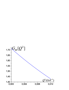
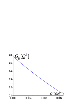
Figure 2: Deuteron electromagnetic form factors defined by Eq. (29) with parameters as in the text.

The energy dependence of the differential cross section for different angles and the angular dependence for different energies are illustrated in Fig. 3. We restrict ourselves by the values: $E\leq$ 200 GeV and $\theta_{e}\leq$ 50 mrad.

The unpolarized differential cross section is divergent at small values of energy, as expected from the one-photon exchange mechanism. It is monotonically decreasing, not presenting minima, when the deuteron energy increases and increases when the electron scattering angle increases.

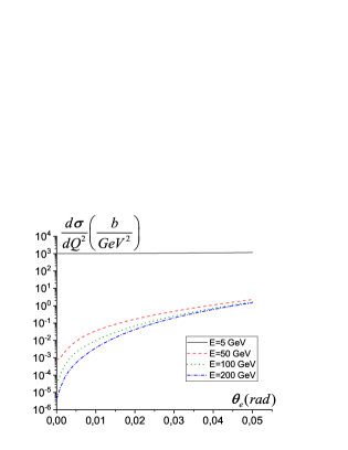
Figure 3: Differential cross section for the unpolarized $d-e$ elastic scattering as defined by Eqs.(26) and (28): as a function of incident deuteron beam energy $E$ for different electron scattering angles (left panel) and as a function of the electron scattering angle at different values of incident energy $E$ (right panel).

III Polarization observables

Several polarization observables can be measured and calculated for elastic deuteron-electron scattering. Besides the electron polarization, the initial and final deuterons may have vector and tensor polarizations. Let us focus here on single and double polarization observables. Among single-spin observables, we consider effects which arise within the one-photon exchange approximation when the amplitude of the process (1) is real. In this respect, we note that in presenc of the two photon exchange contribution, the scattering amplitude contains an imaginary part. Then, other single-spin effects arise, due to the target electron polarization or due to vector polarization of the deuteron beam. They lead to azimuthal asymmetry of the cross section similar to the one in elastic electron-proton scattering [Ref]. Here we consider the single-spin effects due to the tensor polarization of the initial or final deuteron.

1. The analyzing powers (asymmetries) due to the tensor polarization of the deuteron beam, $\vec{d}\,^{T}+e\to d+e$.

2. The tensor polarization of the scattered deuteron when the other particles are unpolarized, $d+e\to\vec{d}\,^{T}+e$.

3. The polarization transfer coefficients which describe the polarization transfer from the polarized electron target to the recoil electron in the $d+\vec{e}\to d+\vec{e}$ reaction.

4. The spin correlation coefficients when the deuteron beam is vectorially polarized and the initial electron has arbitrary polarization, $\vec{d}\,^{V}+\vec{e}\to d+e$.

5. The polarization transfer coefficients which describe the vector polarization transfer from a polarized electron target to the scattered deuteron, $d+\vec{e}\to\vec{d}\,^{V}+e$.

6. The spin correlation coefficients when the scattered deuteron has vector polarization and the final electrons have arbitrary polarization, $d+e\to\vec{d}\,^{V}+\vec{e}$.

7. The polarization transfer coefficients which describe the polarization transfer from the vector-polarized deuteron beam to the recoil electron in the $\vec{d}\,^{V}+e\to d+\vec{e}$ reaction.

8. The depolarization coefficients which define the dependence of the scattered deuteron vector polarization on the vector polarization of the deuteron beam, $\vec{d}\,^{V}+e\to\vec{d}\,^{V}+e$.

Let us choose the following orthogonal system: the $z$ axis is directed along the direction of the deuteron beam momentum $\vec{p}$, the momentum of the recoil electron $\vec{k}_{2}$ lies in the $xz$ plane ($\theta$ is the angle between the deuteron beam and the recoil electron momenta), and the $y$ axis is directed along the vector $\vec{p}\times\vec{k}_{2}$ (see Fig. 1.). So, the components of the deuteron beam and recoil electron momenta are the following

$$p_{x}=p_{y}=0,\ p_{z}=p,\ k_{2x}=k_{2}\sin\theta_{e},\ k_{2y}=0,\ k_{2z}=k_{2}\cos\theta_{e},$$

where $p\,(k_{2})$ is the magnitude of the deuteron beam (recoil electron) momentum.

To calculate the polarization observables it is necessary to define the polarization 3-vectors of all particles as well the components of both deuteron tensor polarizations in their rest frames. In our work we choose the unique coordinate system shown in Fig. 1 (laboratory system) for all these quantities.

The corresponding polarization observables are analytically calculated as functions of $Q^{2}$ at fixed deuteron beam energy and their dependence on the kinematical variables is plotted similarly to the unpolarized cross section in Fig. 3.

III.1 The analyzing powers or asymmetries, $A_{ij}$, due to the tensor polarization of the deuteron beam, $\vec{d}\,^{T}+e\to d+e$.

We consider here the scattering of the tensor polarized deuteron beam on an unpolarized electron target. The hadronic tensor corresponding to a tensor polarized deuteron beam can be written in the following general form

$$H_{\mu\nu}({\cal Q}^{(i)})=H_{3}(Q^{2})\bar{Q}^{(i)}\tilde{g}_{\mu\nu}+H_{4}(Q^{2})\frac{\bar{Q}^{(i)}}{4M^{2}}P_{\mu}P_{\nu}+H_{5}(Q^{2})(P_{\mu}\tilde{Q}^{(i)}_{\nu}+P_{\nu}\tilde{Q}^{(i)}_{\mu})+H_{6}(Q^{2})\tilde{\cal Q}^{(i)}_{\mu\nu},$$ (31)

where

$$\tilde{Q}^{(i)}_{\mu} = {\cal Q}^{(i)}_{\mu\nu}k^{\nu}+\frac{k_{\mu}}{Q^{2}}\bar{Q}^{(i)},~{}\,\tilde{Q}^{(i)}_{\mu}k^{\mu}=0,$$

$$\tilde{Q}^{(i)}_{\mu\nu} = {\cal Q}^{(i)}_{\mu\nu}+\frac{k_{\mu}k_{\nu}}{Q^{4}}\bar{Q}^{(i)}+\frac{k_{\nu}k^{\alpha}}{Q^{2}}{\cal Q}^{(i)}_{\mu\alpha}+\frac{k_{\mu}k^{\alpha}}{Q^{2}}{\cal Q}^{(i)}_{\nu\alpha},$$ (32)

$$\tilde{Q}^{(i)}_{\mu\nu}k^{\nu}=0,~{}\,\bar{Q}^{(i)}={\cal Q}^{(i)}_{\alpha\beta}k^{\alpha}k^{\beta}.$$

The structure functions $H_{i}(k^{2})$ are related to the deuteron electromagnetic form factors by:

$$H_{3}(Q^{2}) = -G_{M}^{2},\,\ H_{4}(Q^{2})=G_{M}^{2}+\frac{4}{1+\tau}G\,G_{Q},\ H_{5}(Q^{2})=-\tau(G_{M}+2G_{Q})G_{M},\$$

$$H_{6}(Q^{2}) = Q^{2}(1+\tau)G_{M}^{2},\,\ G=\tau\,G_{M}+G_{C}+\frac{\tau}{3}\,G_{Q}.$$ (33)

The contraction of the spin independent leptonic $L^{\mu\nu}(0)$ and spin dependent (due to the tensor polarization of the deuteron beam) hadronic $H_{\mu\nu}({\cal Q}^{(i)})$ tensors, in an arbitrary reference frame, gives:

$$C({\cal Q}^{(i)})=L^{\mu\nu}(0)\,H_{\mu\nu}({\cal Q}^{(i)})=a\,k_{1}^{\mu}\,k_{1}^{\nu}\,{\cal Q}^{(i)}_{\mu\nu}+b\,k_{1}^{\mu}\,k^{\nu}\,Q^{(i)}_{\mu\nu}+c\,k^{\mu}\,k^{\nu}\,{\cal Q}^{(i)}_{\mu\nu},$$ (34)

where the functions $a,b$ and $c$ have the following form in terms of the deuteron electromagnetic form factors (in the rest frame of the electron target):

$$a = 4(1+\tau)Q^{2}\,G_{M}^{2},\ b=-16\tau G_{M}\left[(M^{2}+m\,E)G_{M}+2(m\,E-\tau M^{2})\,G_{Q}\right],$$

$$c = [Q^{2}-4m^{2}+4\frac{m^{2}}{M^{2}}E^{2}]\,G_{M}^{2}+16\tau m\,E\,G_{M}\,G_{Q}+$$ (35)

$$+\frac{4}{M^{2}}\frac{G_{Q}\,G}{1+\tau}\left[-Q^{2}(M^{2}+2m\,E)+4m^{2}\,E^{2}\right].$$

From the condition $p_{1}^{\mu}\,{\cal Q}^{(i)}_{\mu\nu}=0$ one can express the time components of the quadrupole polarization tensor in terms of the space components of this tensor. These relations are:

$${\cal Q}^{(i)}_{00}=\frac{p^{2}}{E^{2}}{\cal Q}^{(i)}_{zz},\ \ {\cal Q}^{(i)}_{0x}=\frac{p}{E}{\cal Q}^{(i)}_{xz},\ \ {\cal Q}^{(i)}_{0y}=\frac{p}{E}{\cal Q}^{(i)}_{yz},\ \ {\cal Q}^{(i)}_{0z}=\frac{p}{E}{\cal Q}^{(i)}_{zz}.$$ (36)

The components of the quadrupole polarization tensor ${\cal Q}^{(i)}_{ij}$ defined in the Lab system can be related to the corresponding ones defined in the rest system of the deuteron beam (denoted as $R_{ij}$) by the following relations

$${\cal Q}^{(i)}_{xx}=R_{xx},\ \ {\cal Q}^{(i)}_{yy}=R_{yy},\ \ {\cal Q}^{(i)}_{xz}=\frac{E}{M}\,R_{xz},\ \ {\cal Q}^{(i)}_{zz}=\frac{E^{2}}{M^{2}}\,R_{zz}.$$

The $Q^{2}$ dependence of the differential cross section of the reaction (1) on the polarization characteristics of the deuteron beam, in the case when beam is tensor polarized, has the following form

$$\frac{d\sigma}{dQ^{2}}({\cal Q}^{(i)})=\left(\frac{d\sigma}{dQ^{2}}\right)_{un}\left[1+A_{xx}({\cal Q}_{xx}-{\cal Q}_{yy})+A_{xz}{\cal Q}_{xz}+A_{zz}{\cal Q}_{zz}\right],$$ (37)

where $A_{ij}$, $i,j=x,y,z$ are the analyzing powers (asymmetries) which characterize the $\vec{d}\,^{T}-e$ scattering when the deuteron beam is tensor polarized.

The expressions of these analyzing powers in terms of the deuteron electromagnetic form factors have the following form

$${\cal D}A_{xx} = \frac{x^{2}}{M^{2}}\Big{[}(m^{2}p^{2}+\tau M^{4})G_{M}^{2}+mE\,Q^{2}\,G_{M}\,G_{Q}+\frac{(4m^{2}E^{2}-M^{2}Q^{2}-2mE\,Q^{2})}{1+\tau}\,G_{Q}\,G\Big{]},$$

$${\cal D}A_{xz} = 2\frac{x\tau(M^{2}+mE)}{mpE}\Big{\{}M^{2}Q^{2}\,G_{M}^{2}-2\Big{[}\frac{m^{2}p^{2}(4mE-Q^{2})}{M^{2}+mE}$$

$$-2mE\,Q^{2}\Big{]}\,G_{M}\,G_{Q}+\frac{4(4m^{2}E^{2}-M^{2}Q^{2}-2mE\,Q^{2})}{1+\tau}\,G_{Q}\,G\Big{\}},$$

$${\cal D}A_{zz} = \frac{Q^{2}}{E^{2}}\Big{\{}\Big{[}m^{2}p^{2}\Big{(}1+\frac{Q^{2}}{\,\,\,Q^{2}_{max}}\Big{)}+\frac{Q^{4}}{8}-\frac{3}{4}\,M^{2}\,x^{2}\Big{]}G_{M}^{2}+$$

$$\Big{[}\frac{Q^{4}}{2}+mE\big{[}4\tau(Q^{2}-2mE)-3x^{2}\big{]}\Big{]}G_{M}\,G_{Q}$$

$$+\frac{Q^{2}(M^{2}+2mE)-4m^{2}E^{2}}{1+\tau}\Big{(}1-2\tau-3\frac{Q^{2}}{\,\,\,Q^{2}_{max}}\Big{)}G_{Q}\,G,\Big{\}},$$

$$x = k_{2x}=-p_{2x}=\left[Q^{2}\Big{(}1-\frac{Q^{2}}{\,\,\,Q^{2}_{max}}\Big{)}\right]^{1/2}.$$ (38)

The asymmetries due the tensor polarization of the deuteron beam are plotted in Fig. 4 for the chosen form factors.

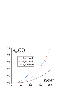
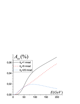
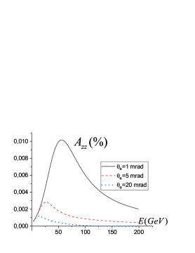
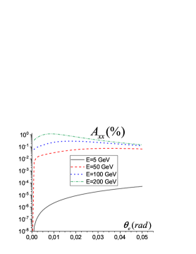
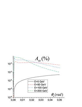
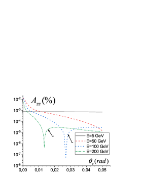
Figure 4: Asymmetries due to tensor polarization of the deuteron beam given by Eqs.(37, 38) as function of the deuteron beam energy $E$ at various values of the electron scattering angle $\theta_{e}$ (upper row) and as function of $\theta_{e}$ at different values $E$ (lower row). The arrow with the sign ”minus” indicates that corresponding asymmetry may become negative and the absolute value is plotted.

III.2 Tensor polarization coefficients, $P_{ij}$, in the $d+e\to\vec{d}\,^{T}+e$ reaction the tensor polarization of the scattered deuteron is measured

We consider here the scattering of an unpolarized deuteron beam on an unpolarized electron target (the polarization of the recoil electron is not measured). In this case the scattered deuterons may acquire a tensor polarization. The hadronic tensor which corresponds to the case of an unpolarized deuteron beam and a tensor polarized scattered deuteron can be written in the following general form

$$H_{\mu\nu}({\cal Q}^{(f)})=\bar{H}_{3}\bar{\cal Q}^{(f)}\tilde{g}_{\mu\nu}+\bar{H}_{4}\frac{\bar{\cal Q}^{(f)}}{4M^{2}}P_{\mu}P_{\nu}-\bar{H}_{5}(P_{\mu}\tilde{\cal Q}^{(f)}_{\nu}+P_{\nu}\tilde{Q}^{(f)}_{\mu})+\bar{H}_{6}\tilde{\cal Q}^{(f)}_{\mu\nu},$$ (39)

where the structure functions $\bar{H}_{i}$, averaged over the spin of the initial deuteron, have the following expressions in the terms of the deuteron electromagnetic form factors: $\bar{H}_{i}=H_{i}/3,i=3,4,5,6$. Note that the tensor structures in this case can be obtained from Eq. (31) by the substitution $(p_{1}\leftrightarrows-p_{2}),$, wherein the structure accompanying $\bar{H}_{5}$ changes sign.

The contraction of the spin independent leptonic $L_{\mu\nu}^{(0)}$ and spin dependent (due to the tensor polarization of the scattered deuteron) hadronic $H_{\mu\nu}(Q^{(f)})$ tensors, in an arbitrary reference frame, gives:

$$C({\cal Q}^{(f)})=L^{\mu\nu}{(0)}H_{\mu\nu}({\cal Q}^{(f)})=\bar{a}\,k_{1}^{\mu}k_{1}^{\nu}{\cal Q}^{(f)}_{\mu\nu}+\bar{b}\,k_{1}^{\mu}p_{1}^{\nu}{\cal Q}^{(f)}_{\mu\nu}+\bar{c}\,k^{\mu}k^{\nu}{\cal Q}^{(f)}_{\mu\nu},$$ (40)

where the coefficients $\bar{a},\bar{b}$ and $\bar{c}$ are written in terms of the deuteron electromagnetic form factors as:

$$\bar{a} = \frac{2}{3}(1+\tau)Q^{2}G_{M}^{2},$$

$$\bar{b} = \frac{8}{3}\tau G_{M}\left[(M^{2}+2\tau M^{2}-k_{1}\cdot p_{1})G_{M}+2(\tau M^{2}-k_{1}\cdot p_{1})G_{Q}\right],$$

$$\bar{c} = \frac{2}{3M^{2}}\{[(k_{1}\cdot p_{1})^{2}-Q^{2}k_{1}\cdot p_{1}-m^{2}M^{2}+\tau(1+4\tau)M^{4}]G_{M}^{2}-k^{2}(2\tau M^{2}-k_{1}\cdot p_{1})G_{M}G_{Q}+$$ (41)

$$+(1+\tau)^{-1}[4(k_{1}\cdot p_{1})^{2}-Q^{2}(M^{2}+2k_{1}\cdot p_{1})]G_{Q}\,G\}.$$

From the condition $p_{2}^{\mu}\,{\cal Q}^{(f)}_{\mu\nu}=0$ one can express the time components of the scattered deuteron quadrupole polarization tensor in terms of the space components of this tensor. These relations are:

$${\cal Q}^{(f)}_{00} = \frac{x^{2}{\cal Q}^{(f)}_{xx}-2xz{\cal Q}^{(f)}_{xz}+z^{2}{\cal Q}^{(f)}_{zz}}{E_{d}^{2}},\ \ {\cal Q}^{(f)}_{0z}=\frac{z{\cal Q}^{(f)}_{zz}-y{\cal Q}^{(f)}_{xz}}{E_{d}},$$ (42)

$${\cal Q}^{(f)}_{0x} = \frac{z{\cal Q}^{(f)}_{xz}-x{\cal Q}^{(f)}_{xx}}{E_{d}},\ \ {\cal Q}^{(f)}_{0y}=\frac{z{\cal Q}^{(f)}_{yz}-x{\cal Q}^{(f)}_{xy}}{E_{d}},\ \ E_{d}=E-\frac{Q^{2}}{2m}$$

where $E_{d}$ is the energy of the scattered deuteron and

$$z=p_{2z}=p\,\Big{[}1-\frac{(E+m)\,Q^{2}}{2m\,p^{2}}\Big{]}.$$

The components of the quadrupole polarization tensor $Q^{(f)}_{ij}$ which are defined in the Lab system can be related to the corresponding ones in the rest system of the scattered deuteron (denote them as $V_{ij}$) by the following relations

$${\cal Q}^{(f)}_{xx} = (1+x^{2}y)^{2}V_{xx}-2xyz(1+x^{2}y)V_{xz}+(xyz)^{2}V_{zz},\ \ {\cal Q}^{(f)}_{yy}=V_{yy},$$ (43)

$${\cal Q}^{(f)}_{zz} = (xyz)^{2}V_{xx}-2xyz(1+z^{2}y)V_{xz}+(1+yz^{2})^{2}V_{zz},$$

$${\cal Q}^{(f)}_{xz} = -xyz(1+z^{2}y)V_{xx}+[1+y(x^{2}+z^{2})+2(xyz)^{2}]V_{xz}-xyz(1+yz^{2})V_{zz},$$

where

$$y=\frac{1}{M(E_{d}+M)}.$$

The dependence of the differential cross section of the reaction (1) on the polarization characteristics of the scattered deuteron (given in the Lab system)in case when the deuteron beam and electron target are unpolarized has the following form

$$\frac{d\sigma}{dQ^{2}}({\cal Q}^{(f)})=\left(\frac{d\sigma}{dQ^{2}}\right)_{un}\left[1+P_{xx}({\cal Q}^{(f)}_{xx}-{\cal Q}^{(f)}_{yy})+P_{xz}{\cal Q}^{(f)}_{xz}+P_{zz}{\cal Q}^{(f)}_{zz}\right],$$ (44)

where $P_{ij}$, $i,j=x,y,z$ are the components of the tensor polarization which describe the $d+e\to\vec{d}\,^{T}+e$ scattering in case when the scattered deuteron is tensor polarized. The explicit expressions of these tensor polarizations, in terms of the deuteron electromagnetic form factors, can be written as

$${\cal D}P_{zz} = \frac{2}{3\,M^{2}d\,E_{d}}\big{[}a_{1}\,G_{M}^{2}+a_{2}\,G_{M}\,G_{Q}+a_{3}\,G_{Q}\,G\big{]},\ \ d=2E_{d}^{2}-x^{2},$$

$$a_{1} = (2z^{2}-x^{2})\,E_{d}\big{\{}E^{2}(m^{2}p^{2}+\tau M^{4})-Q^{2}(E+m)[mp^{2}-\tau M^{2}(E+m)]\big{\}}$$

$$+p\,d\big{[}-mzQ^{2}(M^{2}+2\tau M^{2}-mE)+(pE_{d}-2Ez)(m^{2}p^{2}-mEQ^{2}+\tau M^{4}+\tau M^{2}Q^{2})\big{]},$$

$$a_{2} = Q^{2}\big{\{}-p^{2}d\,m\,E_{d}^{2}-2p\,d\,z[\tau M^{2}(2E+m)-mE(E+m)]+$$

$$+(2z^{2}-x^{2})E\,E_{d}[2\tau M^{2}(E+m)-mE(E+2m)]\big{\}},$$

$$a_{3} = \frac{4m^{2}E^{2}-Q^{2}(M^{2}+2mE)}{1+\tau}\big{[}(2z^{2}-x^{2})E^{2}\,E_{d}+p\,d(p\,E_{d}-2E\,z)\big{]}$$

$${\cal D}P_{xx} = \frac{2\,x^{2}}{3d\,M^{2}}[b_{1}\ G_{M}^{2}+b_{2}\ G_{M}\ G_{Q}+b_{3}\ G_{Q}\,G],$$ (45)

$$b_{1} = mp^{2}[mE^{2}-Q^{2}(E+m)]+\tau M^{2}[E^{2}M^{2}+Q^{2}(E+m)^{2}],$$

$$b_{2} = -EQ^{2}[2(mE-\tau M^{2})(E+m)-mE^{2}],$$

$$b_{3} = \frac{E^{2}}{1+\tau}[4m^{2}E^{2}-Q^{2}(M^{2}+2mE)],$$

$${\cal D}P_{xz} = \frac{2x}{3dM^{2}E_{d}}\big{[}c_{1}G_{M}^{2}+c_{2}G_{M}G_{Q}+c_{3}G_{Q}\,G\big{]},$$

$$c_{1} = 4pQ^{2}(E+m)E_{d}[2mp^{2}-Q^{2}(E+m)]-4zE_{d}\big{[}Q^{2}\tau M^{2}(E+m)^{2}+E^{2}(m^{2}p^{2}+\tau M^{4})$$

$$+p^{2}Q^{2}m(E+m)\big{]}+pd\big{[}2E(m^{2}p^{2}+\tau M^{4}+\tau Q^{2}M^{2})-mQ^{2}(mE+E^{2}+p^{2}-2\tau M^{2})\big{]},$$

$$c_{2} = -4zEQ^{2}E_{d}\big{[}mE^{2}+2(E+m)(\tau M^{2}-mE)\big{]}-pdQ^{2}\big{[}2mE(E+m)-2\tau M^{2}(2E+m)\big{]},$$

$$c_{3} = \frac{2E}{1+\tau}[(4m^{2}E^{2}-Q^{2}(M^{2}+2mE)](pd-2zEE_{d}).$$

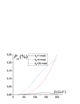
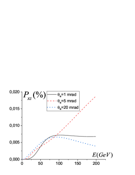
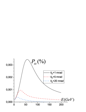
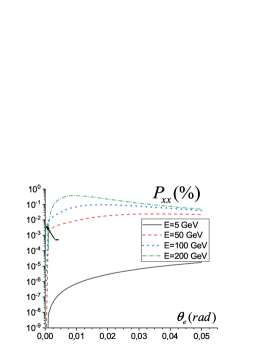
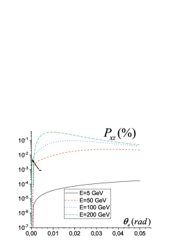
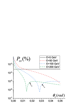
Figure 5: Same as Fig. 4 but for the tensor polarization coefficients $P_{ij}$ given by Eqs. (45), which describe the tensor polarization of the final deuteron when the other particles are unpolarized. When the observable has negative values, its modulus is plotted (indicated by arrows).

The results for the scattered deuteron tensor polarizations are shown in Fig. 5.

III.3 Polarization transfer coefficients from the target to the recoil electron, $t_{ij}$, in the $d+\vec{e}\to d+\vec{e}$ reaction

We consider below the scattering of an unpolarized deuteron beam on a polarized electron target in the case when the polarization of the recoil electron is measured and the polarization of the scattered deuteron is not measured.

The part of the leptonic tensor which corresponds to the case of polarized target and polarized recoil electron has the following form

$$L_{\mu\nu}(s_{1},s_{2}) = -(k_{1}\cdot s_{2}k_{2}\cdot s_{1}-\frac{Q^{2}}{2}s_{1}\cdot s_{2})g_{\mu\nu}-\frac{Q^{2}}{2}(s_{1\mu}s_{2\nu}+s_{1\nu}s_{2\mu})-s_{1}\cdot s_{2}(k_{1\mu}k_{2\nu}+k_{1\nu}k_{2\mu})+$$ (46)

$$k_{1}\cdot s_{2}(s_{1\mu}k_{2\nu}+s_{1\nu}k_{2\mu})+k_{2}\cdot s_{1}(s_{2\mu}k_{1\nu}+s_{2\nu}k_{1\mu}),$$

where $s_{2\mu}$ is the polarization four-vector of the recoil electron which satisfies the following conditions: $k_{2}\cdot s_{2}=0,s_{2}^{2}=-1.$

In the Lab system, where the target electron is at rest, the polarization four-vector of the recoil electron has the following components

$$s_{2}=\left(\frac{\vec{k}_{2}\cdot\vec{\xi}_{2}}{m},\vec{\xi}_{2}+\frac{\vec{k}_{2}(\vec{k}_{2}\cdot\vec{\xi}_{2})}{m(m+\epsilon_{2})}\right),$$ (47)

where $\vec{\xi}_{2}$ is the unit vector describing the polarization of the recoil electron in its rest system and $\epsilon_{2}$ is the recoil electron energy.

The contraction of the spin dependent leptonic tensor $L_{\mu\nu}(s_{1},s_{2})$ and the spin independent hadronic tensor $H_{\mu\nu}(0),$ in an arbitrary reference frame, can be written as follows

$$C(s_{1},s_{2}) = L^{\mu\nu}(s_{1},s_{2})H_{\mu\nu}(0)=-2m^{2}s_{1}\cdot s_{2}H_{1}(Q^{2})+$$ (48)

$$+\frac{H_{2}(Q^{2})}{M^{2}}\Big{\{}-2s_{1}\cdot s_{2}\left[(k_{1}\cdot P)^{2}-\frac{P^{2}Q^{2}}{4}\right]-4M^{2}(1+\tau)k_{1}\cdot s_{2}k_{2}\cdot s_{1}-$$

$$-Q^{2}P\cdot s_{1}P\cdot s_{2}+2P\cdot k_{1}(k_{1}\cdot s_{2}P\cdot s_{1}+k_{2}\cdot s_{1}P\cdot s_{2})\Big{\}},$$

where the structure functions $H_{1,2}(Q^{2})$ are given by Eq. (19).

The dependence of the differential cross section of the reaction $d+\vec{e}\to d+\vec{e}$ on the polarizations of the initial and recoil electrons has the following form

$$\frac{d\sigma}{dQ^{2}}(\vec{\xi}_{1},\vec{\xi}_{2})=\frac{1}{2}\left(\frac{d\sigma}{dQ^{2}}\right)_{un}\left[1+t_{xx}\xi_{1x}\xi_{2x}+t_{yy}\xi_{1y}\xi_{2y}+t_{zz}\xi_{1z}\xi_{2z}+t_{xz}\xi_{1x}\xi_{2z}+t_{zx}\xi_{1z}\xi_{2x}\right],$$ (49)

where $t_{ij}$, $i,j=x,y,z$ are the coefficients of the polarization transfer from the initial electron to the recoil one.

The explicit expressions of the polarization transfer coefficients, as functions of the deuteron form factors, in the Lab system can be written as

$$Dt_{xx} = (2m^{2}+Q^{2}\sin^{2}\theta_{e})\Big{\{}H_{1}(Q^{2})+4\frac{H_{2}(Q^{2})}{M^{2}}[E^{2}-\lambda(M^{2}+2mE)]\Big{\}}+$$ (50)

$$+\frac{4H_{2}(Q^{2})|\vec{k}_{2}|\,\sin^{2}{\theta_{e}}}{M^{2}}\big{[}4\lambda mpE\cos{\theta_{e}}+|\vec{k}_{2}|(M^{2}-2E^{2})\big{]},$$

$$Dt_{yy} = 2m^{2}\Big{\{}H_{1}(Q^{2})+4\frac{H_{2}(Q^{2})}{M^{2}}[E^{2}-\lambda(M^{2}+2mE)]\Big{\}},$$

$$Dt_{zz} = 4|\vec{k}_{2}|\cos\theta_{e}\frac{H_{2}(Q^{2})}{M^{2}}[(M^{2}-2E^{2})|\vec{k}_{2}|cos\theta_{e}+4\lambda mp(m+E+E\cos^{2}\theta_{e})]+$$

$$+2m^{2}(1+2\lambda\cos^{2}\theta_{e})\Big{\{}H_{1}(Q^{2})+4\frac{H_{2}(Q^{2})}{M^{2}}[E^{2}-\lambda(2E^{2}-M^{2}+2mE)]\Big{\}},$$

$$Dt_{xz} = 4|\vec{k}_{2}|\sin\theta_{e}\frac{H_{2}(Q^{2})}{M^{2}}[(M^{2}-2E^{2})|\vec{k}_{2}|\cos\theta_{e}+2mpE]+$$

$$+4\lambda\cos\theta_{e}\sin\theta_{e}\Big{\{}m^{2}H_{1}(Q^{2})+\frac{H_{2}(Q^{2})}{M^{2}}[4mE(mE+p|\vec{k}_{2}|\cos\theta_{e})-Q^{2}(M^{2}+2mE)]\Big{\}},$$

$$Dt_{zx} = 4|\vec{k}_{2}|\sin\theta_{e}\frac{H_{2}(Q^{2})}{M^{2}}[(M^{2}-2E^{2})|\vec{k}_{2}|\cos\theta_{e}+2mp(2m\lambda+2\lambda E-E)]+$$

$$+4\lambda\cos\theta_{e}\sin\theta_{e}\Big{\{}m^{2}H_{1}(Q^{2})+\frac{H_{2}(Q^{2})}{M^{2}}[4mE(mE+p|\vec{k}_{2}|\cos\theta_{e})-Q^{2}(E^{2}+p^{2}+2mE)]\Big{\}},$$

where $\lambda=Q^{2}/(4m^{2})$. Let us remind that $\sin{\theta_{e}}$ and $\cos{\theta_{e}}$ are functions of $Q^{2}$ and of the deuteron beam energy $E,$ namely

$$|\vec{k}_{2}|\cos\theta_{e}=\frac{Q^{2}}{2m}\sqrt{1+\frac{4m^{2}}{Q^{2}_{max}}},\ |\vec{k}_{2}|\sin\theta_{e}=\sqrt{Q^{2}\bigg{(}1-\frac{Q^{2}}{Q^{2}_{max}}\bigg{)}},\ |\vec{k}_{2}|=\sqrt{Q^{2}(1+\lambda)}.$$

The expression for $Q^{2}_{max}$ is given in Eq. (6).

The electron polarization transfer coefficients $t_{ij}$ are plotted in Fig. 6.

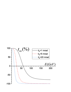
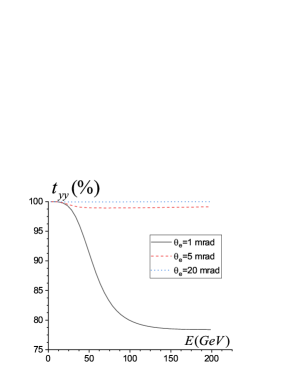
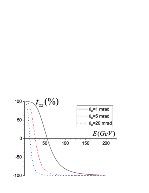
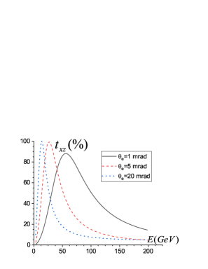
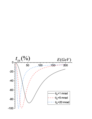
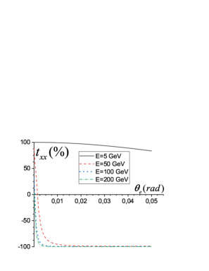
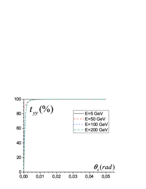
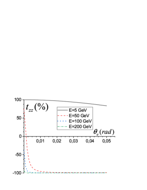
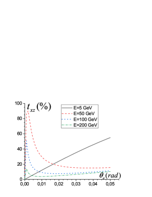
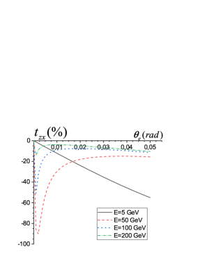
Figure 6: Coefficients of the polarization transfer from the target to the recoil electron in $d+e$ elastic scattering given by Eqs. (50).

III.4 Spin correlation coefficients, $C_{ij}$ due to a polarized electron target and a vector polarized deuteron beam: $\vec{d}\,^{V}+\vec{e}\to d+e$

Let us consider the scattering of a vector polarized deuteron beam (the polarizations of the final particles are not detected). In this case a non-zero polarization effects arise only when the electron target is also polarized. So, the part of the hadronic tensor $H_{\mu\nu}(\eta_{1})$ related to the vector polarized deuteron beam and unpolarized scattered deuteron can be written as:

$$H_{\mu\nu}(\eta_{1}) = 2iM\,G_{M}\Big{[}(1+\tau)\widetilde{G}<\mu\nu\eta_{1}k>+\frac{\eta_{1}\cdot k}{4M^{2}}(G_{M}-2\widetilde{G})<\mu\nu p_{1}k>\Big{]},$$

$$\widetilde{G} = G_{C}+\frac{\tau}{3}G_{Q}.$$ (51)

One can see that all correlation coefficients in $\vec{d}\,^{V}+\vec{e}\to d+e$, and polarization transfer coefficients in the reaction $d+\vec{e}\to\vec{d}\,^{V}+e$, when the deuteron is vector polarized, are proportional to the deuteron magnetic form factor. It is also true for the $e+d$ elastic scattering for the corresponding polarization observables.

The contraction of the spin-dependent leptonic $L_{\mu\nu}^{(p)}(s_{1})$ and hadronic $H_{\mu\nu}(\eta_{1})$ tensors, in an arbitrary reference frame, gives:

$$C(s_{1},\eta_{1}) = L_{\mu\nu}^{(p)}(s_{1})H^{\mu\nu}(\eta_{1})=4mMG_{M}\{\tau k\cdot\eta_{1}(k\cdot s_{1}+2p_{1}\cdot s_{1})G_{M}+$$ (53)

$$+2\,\widetilde{G}\,[Q^{2}(1+\tau)s_{1}\cdot\eta_{1}+k\cdot\eta_{1}(k\cdot s_{1}-2\tau p_{1}\cdot s_{1})]\}.$$

In the considered frame, where the target electron is at rest, the polarization four-vectors of the electron target and of the deuteron beam have the following components

$$s_{1}=(0,\vec{\xi}_{1}),\ \ \eta_{1}=\left(\frac{\vec{p}\cdot\vec{S}_{1}}{M},\vec{S}_{1}+\frac{\vec{p}(\vec{p}\cdot\vec{S}_{1})}{M(E+M)}\right),$$ (54)

where $\vec{S}_{1}$ is the unit vector describing the vector polarization of the deuteron beam in its rest system.

Applying the P-invariance of the hadron electromagnetic interaction, one can write the following expression for the dependence of the differential cross section on the polarization of the initial particles:

$$\frac{d\sigma}{dQ^{2}}(\vec{\xi}_{1},\vec{S}_{1})=\left(\frac{d\sigma}{dQ^{2}}\right)_{un}\left[1+C_{xx}\xi_{1x}S_{1x}+C_{yy}\xi_{1y}S_{1y}+C_{zz}\xi_{1z}S_{1z}+C_{xz}\xi_{1x}S_{1z}+C_{zx}\xi_{1z}S_{1x}\right],$$ (55)

where $C_{ij}$, $i,j=x,y,z$ are the spin correlation coefficients which determine the $\vec{d}\,^{V}-\vec{e}$ scattering, when the deuteron beam is vector polarized and electron target is arbitrarily polarized.

The explicit expressions of the spin correlation coefficients, as a function of the deuteron form factors is:

$${\cal D}C_{yy} = -4mMQ^{2}(1+\tau)G_{M}\,\widetilde{G},$$

$${\cal D}C_{xx} = 2\tau mMG_{M}\left[x^{2}\,G_{M}-2Q^{2}\left(1+\frac{4M^{2}}{Q^{2}_{max}}\right)\,\widetilde{G}\right],$$

$${\cal D}C_{xz} = \frac{Q^{2}}{p}(mE+M^{2})\,x\,G_{M}\,(\tau G_{M}+2\widetilde{G}),$$

$${\cal D}C_{zx} = -4m\,M\,p\,x\,G_{M}\Big{[}\tau(G_{M}-2\widetilde{G})-\frac{Q^{2}(E+m)}{4mp^{2}}\,(\tau G_{M}+2\widetilde{G})\Big{]},$$

$${\cal D}C_{zz} = -2Q^{2}G_{M}\Big{[}2(mE-\tau M^{2})\,\widetilde{G}+\tau(M^{2}+mE)G_{M}-$$ (57)

$$-\frac{\tau(E+m)M^{2}}{mp^{2}}\,(M^{2}+mE)\,\Big{(}\tau G_{M}+2\,\widetilde{G})\Big{]}.$$

The spin correlation coefficient $C_{ij}$ between the vector polarizations of the target electron and the deuteron beam are shown in Fig. 7.

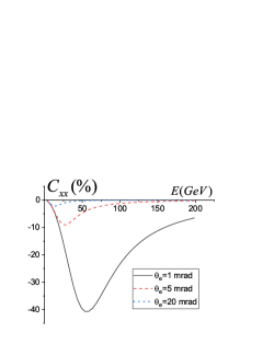
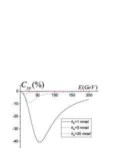
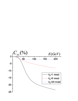
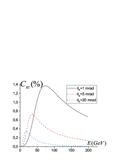
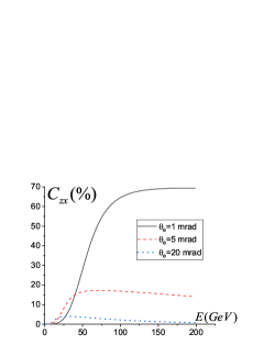
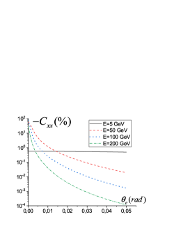
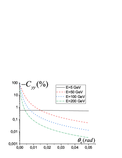
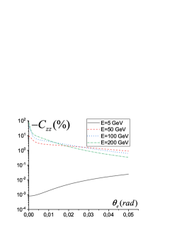
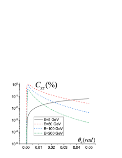
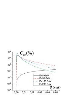
Figure 7: Spin correlation coefficients due to a polarized electron target and a vector polarized deuteron beam, as given in Eqs.  (55, 57).

III.5 Polarization transfer coefficients, $T_{ij}$, in the $d+\vec{e}\to\vec{d}\,^{V}+e$ reaction when the target electron has arbitrary polarization and the vector polarization of the scattered deuteron is measured

Let us consider the case when the initial electron is arbitrary polarized and the scattered deuteron is vectorially polarized. The part of the hadron tensor $H_{\mu\nu}(\eta_{2})$ related to the vector polarized scattered deuteron and unpolarized deuteron beam can be obtained from (51) with the substitutions: $\eta_{1}\to\eta_{2}$ and $p_{1}\leftrightarrows-p_{2}$ and the multiplication by a factor 1/3. The same procedure applies to the calculation of the convolution of the spin depended parts of lepton and hadron tensors. Therefore we have

$$C(s_{1},\eta_{2}) = L_{\mu\nu}^{(p)}(s_{1})H^{\mu\nu}(\eta_{2})=\frac{4}{3}mMG_{M}\{\tau k\cdot\eta_{2}(k\cdot s_{1}-2p_{2}\cdot s_{1})G_{M}+$$ (58)

$$+2\,\widetilde{G}\left[Q^{2}(1+\tau)s_{1}\cdot\eta_{2}+k\cdot\eta_{2}(k\cdot s_{1}+2\tau p_{2}\cdot s_{1})\right]\}.$$

In Lab system the 4-vector $\eta_{2}$ is

$$\eta_{2}=\left(\frac{\vec{p}_{2}\cdot\vec{S}_{2}}{M},\vec{S}_{2}+\frac{\vec{p}_{2}(\vec{p}_{2}\cdot\vec{S}_{2})}{M(E_{d}+M)}\right),$$ (59)

where $\vec{S}_{2}$ is the 3-vector of the scattered deuteron polarization in its rest frame.

The differential cross section can be written as

$$\frac{d\sigma}{dQ^{2}}(\vec{\xi}_{1},\vec{S}_{2})=\left(\frac{d\sigma}{dQ^{2}}\right)_{un}\left[1+T_{xx}\xi_{1x}S_{2x}+T_{yy}\xi_{1y}S_{2y}+T_{zz}\xi_{1z}S_{2z}+T_{xz}\xi_{1x}S_{2z}+T_{zx}\xi_{1z}S_{2x}\right],$$ (60)

where $T_{ij}$, $i,j=x,y,z$ are the polarization transfer coefficients which describe the transfer of polarization from the initial electron to the scattered deuteron.

The explicit expressions of the polarization transfer coefficients, in terms of the deuteron form factors read:

$${\cal D}T_{yy} = -\frac{4}{3}Q^{2}mM(1+\tau)G_{M}\,\widetilde{G},$$

$${\cal D}T_{xx} = \frac{2}{3}mM\,G_{M}\Big{\{}x^{2}yM\big{[}2(M+E+2\tau E)\widetilde{G}-\tau(M+E+2\tau M)G_{M}\big{]}-2Q^{2}(1+\tau)\widetilde{G}\Big{\}},$$

$${\cal D}T_{zx} = \frac{xyM^{2}\,G_{M}}{3p}\big{\{}(E+M+2\tau M)[m(4p^{2}-Q^{2})-Q^{2}E]\tau\,G_{M}-$$

$$-2E\big{[}4m\tau(p^{2}-EM)-Q^{2}(M+E+2\tau E)-Q^{2}m(1+2\tau)\big{]}\big{\}},$$

$${\cal D}T_{xz} = \frac{xm}{3}\Big{\{}\frac{\tau Q^{2}\,G_{M}}{mp}\big{[}m(E+m)-yM(E+M)(m+M)^{2}\big{]}G_{M}$$

$$+4M\big{[}(1+2\tau)[p-yzM(M+E)]+\frac{yzQ^{2}}{2}\big{]}\widetilde{G}\Big{\}},$$

$${\cal D}T_{zz} = -\frac{Q^{2}\,G_{M}}{3}\Big{\{}\frac{\tau(z+p)}{p}\big{[}m(E+m)-yM(E+M)(m+M)^{2}\big{]}G_{M}$$ (61)

$$+\frac{E}{m}\Big{[}Q^{2}\big{[}y(m+M)^{2}+yz(m+M)\frac{E+m}{p}-\frac{(E+m)^{2}}{p^{2}}-\frac{m}{M}\big{]}+4m^{2}\Big{]}\widetilde{G}\Big{\}}.$$

The corresponding transfer coefficients are plotted in Fig. 8.

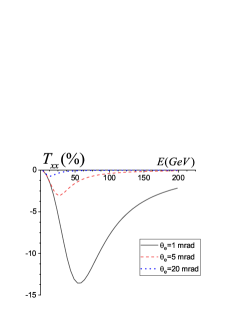
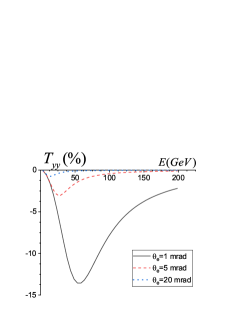
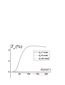
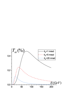
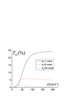
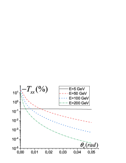
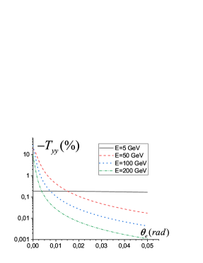
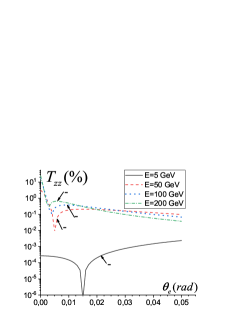
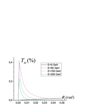
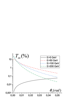
Figure 8: Polarization transfer coefficients from the target electron to the scattered deuteron, given by Eqs. (61), when the target electron has arbitrary polarization and the vector polarization of the scattered deuteron is measured.

III.6 Polarization coefficients, $c_{ij}$, which describe the correlation between the vector polarization of the scattered deuteron and the arbitrary polarization of the recoil electron in the $d+e\to\vec{d}\,^{V}+\vec{e}$ reaction

The scattering of an unpolarized deuteron beam by unpolarized electrons is considered here. In this case a correlation exists between the vector polarization of the scattered deuteron and polarization of the recoil electron. The part of the hadronic tensor $H_{\mu\nu}(\eta_{2})$ related to the vector polarized scattered deuteron and unpolarized deuteron beam can be obtained from Eq. (51) by the substitutions $\eta_{1}\to\eta_{2}$ and $p_{1}\rightleftarrows-p_{2}$, so that:

$$H_{\mu\nu}(\eta_{1})=2iM\,G_{M}\Big{[}(1+\tau)\widetilde{G}<\mu\nu\eta_{2}k>-\frac{\eta_{2}\cdot k}{4M^{2}}(G_{M}-2\widetilde{G})<\mu\nu p_{2}k>\Big{]}.$$ (62)

The leptonic tensor, $L_{\mu\nu}$, which corresponds to an unpolarized initial electron target and polarized recoil electron, has the form:

$$L_{\mu\nu}=\frac{1}{2}\big{[}L_{\mu\nu}^{(0)}+L_{\mu\nu}^{(p)}(s_{2})\big{]},\ \ L_{\mu\nu}^{(p)}(s_{2})=2im\epsilon_{\mu\nu\rho\sigma}k_{\rho}s_{2\sigma}.$$ (63)

The contraction of the spin-dependent leptonic $L_{\mu\nu}^{(p)}(s_{2})$ and hadronic $H_{\mu\nu}(\eta_{2})$ tensors, in an arbitrary reference frame, gives:

$$C(s_{2},\eta_{2})=L_{\mu\nu}^{(p)}(s_{2})H_{\mu\nu}(\eta_{2})=-\frac{4}{3}mMG_{M}\big{\{}\tau k\cdot\eta_{2}(2p_{2}\cdot s_{2}-k\cdot s_{2})G_{M}+$$ (64)

$$+2\left(G_{C}+\frac{\tau}{3}G_{Q}\right)\left[k^{2}(1+\tau)s_{2}\cdot\eta_{2}-k\cdot\eta_{2}(k\cdot s_{2}+2\tau p_{2}\cdot s_{2})\right]\big{\}}.$$

One can see that all the spin correlation coefficients in $d+e\to\vec{d}^{V}+\vec{e}$ reaction, when the scattered deuteron has vector polarization and the recoil electron has arbitrary polarization, are proportional to the deuteron magnetic form factor. It is also true for the $\vec{d}^{V}+e\to d+\vec{e}$ reaction as well for the $ed$ scattering for the corresponding polarization observables.

The differential cross section can be written as:

$$\frac{d\sigma}{dQ^{2}}(\vec{S}_{2},\vec{\xi}_{2})=\frac{1}{2}\left(\frac{d\sigma}{dQ^{2}}\right)_{un}\left[1+c_{xx}S_{2x}\xi_{2x}+c_{yy}S_{2y}\xi_{2y}+c_{zz}S_{2z}\xi_{2z}+c_{xz}S_{2x}\xi_{2z}+c_{zx}S_{2z}\xi_{2x}\right].$$ (65)

The explicit expressions of the corresponding correlation coefficients $c_{ij}$ are

$${\cal D}c_{yy} = -\frac{4}{3}Q^{2}mM(1+\tau)\,G_{M}\,\widetilde{G},$$ (66)

$${\cal D}c_{xx} = \frac{M}{6m(1+\lambda)}\big{(}B_{xx}\,G_{M}^{2}+4\tilde{B}_{xx}\,G_{M}\widetilde{G}\big{)},$$

$$B_{xx} = yx^{2}M\tau[Q^{2}-4m(2E+m)][E+(1+2\tau)M],$$

$$\tilde{B}_{xx} = 2yx^{2}M[(1+2\tau)E+M](m^{2}-\tau M^{2})+2y\tau m[E(E-M)-2(1+\tau)M^{2}]-$$

$$-2(1+\lambda)(1+\tau)Q^{2}m^{2},$$

$${\cal D}c_{xz} = \frac{4xy\tau M^{2}}{3m^{2}p(1+\lambda)}\big{(}B_{xz}\,G_{M}^{2}-2\tilde{B}_{xz}\,G_{M}\widetilde{G}\big{)},$$

$$B_{xz} = [E+(1+2\tau)M]\big{\{}m[m^{2}p^{2}-\tau M^{2}(mE+M^{2})]-\tau M^{2}(E+m)[m(E+m)-\tau M^{2}]\big{\}},$$

$$\tilde{B}_{xz} = \tau EM^{4}[E(1+2\tau)+M]+m^{3}[E^{2}(E-M)-2E(1+\tau)M^{2}]+$$

$$+m^{2}M^{2}[4\tau(1+\tau)M^{2}-(1-2\tau)EM-E^{2}(1+4\tau)]+$$

$$+\tau mM^{2}[2M^{3}+2EM^{2}(2+3\tau)-E^{2}(E-M)],$$

$${\cal D}c_{zx} = \frac{4xy\tau M^{3}}{3m^{2}p(1+\lambda)}\big{(}B_{zx}\tau G_{M}^{2}-2\tilde{B}_{zx}\,\widetilde{G}\big{)},$$

$$B_{zx} = [\tau M^{2}-m(2E+m)]\{M^{2}[E(1+2\tau)+2m(1+\tau)+M]-mE(E-m)\},$$

$$\tilde{B}_{zx} = [E+(1+2\tau)M][\tau M^{4}-mE(m^{2}-3\tau M^{2})]+$$

$$+m^{2}\{(1+2\tau)M[(1+2\tau)M^{2}-E(2E-M)]-2E^{2}\},$$

$${\cal D}c_{zz} = \frac{8y\tau M^{3}}{3m^{3}p^{2}(1+\lambda)}\big{(}B_{zz}\tau\,G_{M}^{2}-2[E+(1+2\tau)M]G_{M}\,\widetilde{G}\big{)},$$

$$B_{zz} = \{M^{2}[E(1+2\tau)+2m(1+\tau)+M]-mE(E-M)\}\times$$

$$\{m^{3}p^{2}-\tau M^{2}[(E+m)(mE+m^{2}-\tau M^{2})+m(mE+M^{2})]\},$$

$$\tilde{B}_{zz} = m^{4}E(p^{2}-\tau M^{2})+\tau m^{2}M^{2}[M^{2}(5\tau E+2(1+\tau)m)-E^{2}(E+4m)]+$$

$$+\tau M^{4}[EM^{2}+2m(E^{2}+M^{2})].$$

The correlation coefficients $c_{ij}$ between the vector polarizations of the scattered deuteron and the recoil electron are shown in Fig. 9.

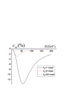
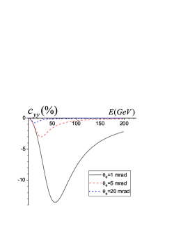
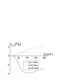
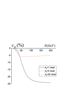
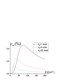
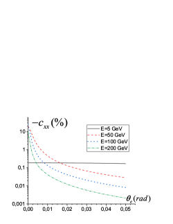
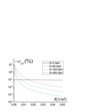
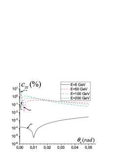
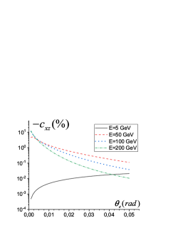
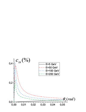
Figure 9: Correlation coefficients due the vector polarizations of the scattered deuteron and the recoil electron in $d+e$ scattering, as given by Eqs. (66).

III.7 Polarization transfer coefficients $\widetilde{T}_{ij}$ which describe arbitrary polarization of the recoil electron when initial deuteron has the vector polarization in the $e+\vec{d}\,^{V}\to\vec{e}+d$ reaction.

The vector polarization transfer from the initial vector polarized deuteron to the recoil electron is calculated below. In this case the polarization dependent part of the hadronic tensor is defined by Eq. (51) and the corresponding part of the leptonic one by Eq. (63). The convolution of these polarization dependent terms can be obtained from $C(s_{1},\eta_{1})$ (see Eq. (53)) by the substitution $s_{1}\to s_{2}.$

The corresponding differential cross section can be written in terms of the polarization transfer coefficients $\widetilde{T}_{ij}$ as :

$$\frac{d\,\sigma}{d\,Q^{2}}=\frac{1}{2}\Big{(}\frac{d\,\sigma}{d\,Q^{2}}\Big{)}_{un}\big{[}1+S_{1x}\xi_{2x}\widetilde{T}_{xx}+S_{1y}\xi_{2y}\widetilde{T}_{yy}+S_{1z}\xi_{2z}\widetilde{T}_{zz}+S_{1x}\xi_{2z}\widetilde{T}_{xz}+S_{1z}\xi_{2x}\widetilde{T}_{zx}\big{]}.$$ (67)

The explicit expressions of the $\widetilde{T}_{ij}$ are

$${\cal D}\widetilde{T}_{yy} = -4mMQ^{2}(1+\tau)\,G_{M}\,\widetilde{G},$$

$${\cal D}\widetilde{T}_{xx} = 4mM\Big{\{}x^{2}\tau\Big{(}\frac{E+m}{m(1+\lambda)}-\frac{1}{2}\Big{)}G_{M}^{2}-\Big{[}x^{2}\Big{(}1+\frac{2(\tau E-m)}{m(1+\lambda)}\Big{)}+Q^{2}(1+\tau)\Big{]}G_{M}\,\widetilde{G}\Big{\}},$$

$${\cal D}\widetilde{T}_{zz} = \frac{8\tau M^{2}}{m^{2}}\Big{\{}\Big{[}mE(\tau M^{2}-m^{2})-m^{2}M^{2}(1-\tau)+,$$

$$+\frac{M^{2}(E+m)^{2}}{p^{2}}\Big{(}2M^{2}-mE-\frac{2\tau(\tau M^{4}-m^{3}E)}{m^{2}(1+\lambda)}\Big{)}\Big{]}\tau G_{M}^{2}+$$

$$+\Big{[}2\tau m^{2}M^{2}+mE(\tau M^{2}-m^{2})+,$$

$$+\frac{\tau M^{2}(E+m)^{2}}{p^{2}}\Big{(}\frac{2(m^{3}E+\tau M^{4})}{m^{2}(1+\lambda)}-mE-2\tau M^{2}\Big{)}\Big{]}2\,G_{M}\,\widetilde{G}\Big{\}},$$

$${\cal D}\widetilde{T}_{xz} = 4\tau xM\Big{\{}\Big{[}\frac{\tau M^{2}(E+m)}{p}\Big{(}\frac{2(E+m)}{m(1+\lambda)}-1\Big{)}-mp\Big{]}G_{M}^{2}+,$$

$$2\Big{[}mp-\frac{M^{2}(E+m)}{p}\Big{(}\frac{2m(\tau E-m)}{m^{2}(1+\lambda)}+1\Big{)}\Big{]}G_{M}\,\widetilde{G}\Big{\}},$$

$${\cal D}\widetilde{T}_{zx} = \frac{4\tau xM^{2}}{p}\Big{\{}\Big{[}M^{2}-Em+\frac{2M^{2}E}{m}+\frac{2(E+m)(m^{3}E-\tau M^{4})}{m^{3}(1+\lambda)}\Big{]}\tau G_{M}^{2}+$$

$$2\Big{[}M^{2}(1-2\tau)-mE-\frac{2\tau M^{2}E}{m}+\frac{2(E+m)(m^{3}E+\tau^{2}M^{4})}{m^{3}(1+\lambda)}\Big{]}G_{M}\,\widetilde{G}\Big{\}}.$$

The polarization transfer coefficients $\widetilde{T}_{ij}$ are plotted in Fig. 10.

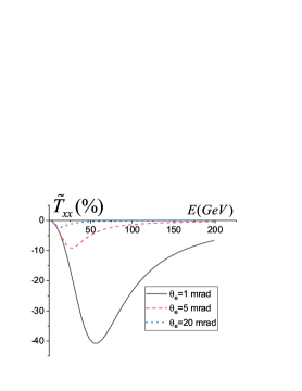
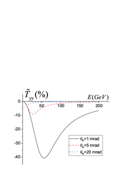
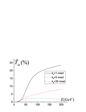
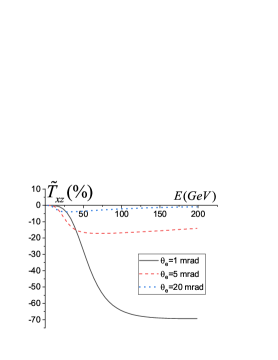
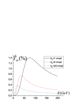
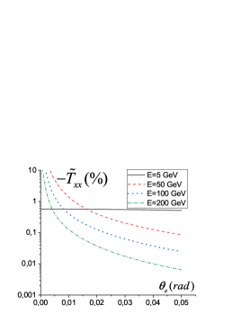
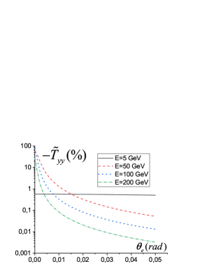
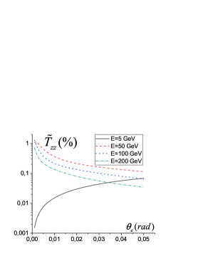
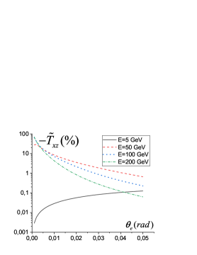
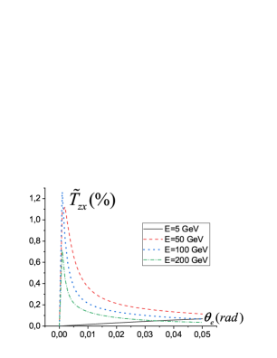
Figure 10: Polarization transfer coefficients which describe arbitrary polarization of the recoil electron when initial deuteron has the vector polarization in the $e+\vec{d}\,^{V}\to\vec{e}+d$ reaction given by Eqs. (III.7).

III.8 Polarization transfer coefficients $V_{ij}$ describing the vector polarization transfer from the initial to the scattered deuteron in the reaction $\vec{d}\,^{V}+e\to\vec{d}\,^{V}+e.$

The scattering of a vector polarized deuteron beam on an unpolarized electron target is considered here. In this case the scattered deuterons can be vector polarized. The hadronic tensor which describes the case of the vector polarized deuteron beam and scattered deuteron can be written as

$$H_{\mu\nu}(\eta_{1},\eta_{2}) = V_{1}\tilde{g}_{\mu\nu}+V_{2}P_{\mu}P_{\nu}+V_{3}(\tilde{\eta}_{1\mu}\tilde{\eta}_{2\nu}+\tilde{\eta}_{1\nu}\tilde{\eta}_{2\mu})++V_{4}(P_{\mu}\tilde{\eta}_{1\nu}+$$ (69)

$$+P_{\nu}\tilde{\eta}_{1\mu})+V_{5}(P_{\mu}\tilde{\eta}_{2\nu}+P_{\nu}\tilde{\eta}_{2\mu}),\ \ \tilde{\eta}_{i\mu}=\eta_{i\mu}-\frac{k\cdot\eta_{i}}{k^{2}}k_{\mu},$$

where the structure functions $V_{i}$ have the following expressions in the terms of the deuteron electromagnetic FFs

$$V_{1} = \frac{1}{2}G_{M}^{2}[(1+2\tau)k\cdot\eta_{1}k\cdot\eta_{2}+4\tau(1+\tau)M^{2}\eta_{1}\cdot\eta_{2}],$$ (70)

$$V_{2} = -\frac{1}{8M^{2}}(1+\tau)^{-1}\{(2G_{C}-\frac{4}{3}\tau G_{Q})[(G_{C}+\frac{4}{3}\tau G_{Q})(k\cdot\eta_{1}k\cdot\eta_{2}+2(1+\tau)M^{2}\eta_{1}\cdot\eta_{2})+$$

$$+(G_{Q}-G_{M})k\cdot\eta_{1}k\cdot\eta_{2}]+(1+\tau)G_{M}^{2}(k\cdot\eta_{1}k\cdot\eta_{2}+4\tau M^{2}\eta_{1}\cdot\eta_{2})\},$$

$$V_{3} = -\tau(1+\tau)M^{2}G_{M}^{2},\ \ V_{4}=-\frac{1}{4}k\cdot\eta_{2}G_{M}(G_{C}+\tau G_{M}-\frac{2}{3}\tau G_{Q}),$$

$$V_{5} = \frac{1}{4}k\cdot\eta_{1}G_{M}(G_{C}+\tau G_{M}-\frac{2}{3}\tau G_{Q}).$$

For this configuration of the hadron polarizations it is sufficient to have an unpolarized electron target since the hadronic tensor in this case is symmetrical over $\mu,\nu$ indices. Thus, the contraction of the spin independent $L_{\mu\nu}^{(0)}$ and spin dependent hadronic $H_{\mu\nu}(\eta_{1},\eta_{2})$ tensors, gives the following expression which is valid in an arbitrary reference frame

$$C(\eta_{1},\eta_{2}) = \frac{4}{M^{2}}G_{M}^{2}\{(k\cdot\eta_{1}k\cdot\eta_{2}-k^{2}\eta_{1}\cdot\eta_{2})[p_{1}\cdot k_{1}(2\tau M^{2}-p_{1}\cdot k_{1})+M^{2}((1+\tau)m^{2}-\tau^{2}M^{2})]+$$ (71)

$$+\tau M^{2}[m^{2}-(1+\tau)M^{2}]k\cdot\eta_{1}k\cdot\eta s_{2}+2\tau M^{2}[(M^{2}+p_{1}\cdot k_{1})k\cdot\eta_{1}k\cdot\eta_{2}+$$

$$+((1+2\tau)M^{2}-p_{1}\cdot k_{1})k_{1}\cdot\eta_{1}k\cdot\eta_{2}-2(1+\tau)M^{2}k_{1}\cdot\eta_{1}k_{1}\cdot\eta_{2}]\}+$$

$$+\frac{8}{(1+\tau)M^{2}}(G_{C}-\frac{2}{3}\tau G_{Q})\{G_{M}(\tau M^{2}-p_{1}\cdot k_{1})[k\cdot\eta_{1}k\cdot\eta_{2}(\tau M^{2}-p_{1}\cdot k_{1})-$$

$$-(1+\tau)M^{2}(k\cdot\eta_{1}k_{1}\cdot\eta_{2}-k_{1}\cdot\eta_{1}k\cdot\eta_{2})]+[\tau M^{4}+2\tau M^{2}p_{1}\cdot k_{1}-(p_{1}\cdot k_{1})^{2}]$$

$$[2(1+\tau)M^{2}(G_{C}+\frac{4}{3}\tau G_{Q})\eta_{1}\cdot\eta_{2}+(G_{C}+(1+\frac{4}{3}\tau)G_{Q})k\cdot\eta_{1}k\cdot\eta_{2}]\}.$$

The corresponding differential cross section is

$$\frac{d\sigma}{dQ^{2}}=\Big{(}\frac{d\sigma}{dQ^{2}}\Big{)}_{un}\big{[}1+V_{xx}S_{1x}S_{2x}+V_{yy}S_{1y}S_{2y}+V_{zz}S_{1z}S_{2z}+V_{xz}S_{1x}S_{2z}+V_{zx}S_{1z}S_{2x}\big{]}.$$ (72)

The explicit expressions for $V_{ij}$ are

$${\cal D}V_{xx} = 2h\Big{\{}\frac{x^{2}}{(1+\tau)M^{3}}\big{[}E-yM(p(p-z)+2(1+\tau)M^{2})\big{]}-2\Big{\}}G^{(-)}\,G^{(+)}+$$

$$\frac{2x^{2}(\tau M^{2}-mE)}{(1+\tau)M^{3}}\big{[}yMp(z-p)(\tau M^{2}-mE)+\tau M^{2}(E+m)-mp^{2}\big{]}G_{M}\,G^{(-)}+$$

$$\big{\{}Q^{2}[\tau M^{2}(\tau M^{2}-2mE-m^{2})+m^{2}p^{2}]$$

$$-x^{2}yM\big{[}\tau M^{4}(M+(1+2\tau)E)+mp^{2}(m(E+M)-2\tau M^{2})\big{]}\big{\}}\frac{G_{M}^{2}}{M^{2}},$$

$${\cal D}V_{yy} = -4hG^{(-)}\,G^{(+)}+[\tau M^{2}(\tau M^{2}-2mE-m^{2})+m^{2}p^{2}]\tau G_{M}^{2},$$

$${\cal D}V_{zz} = \frac{yM}{m^{2}p^{2}}\Big{\{}\frac{4(E-M)hh_{2}}{1+\tau}G^{(-)}\,G^{(+)}-4\tau M^{4}[E+(1+2\tau)M][h+(1+\tau)m^{2}M^{2}]G_{M}^{2}$$

$$-2Q^{2}(E-M)(\tau M^{2}-mE)[h+(1+\tau)m^{2}M^{2}]\frac{h_{1}\,G_{M}\,G^{(-)}}{(1+\tau)M^{2}}\Big{\}},$$

$${\cal D}V_{xz} = \frac{xyM}{mp}\Big{\{}\frac{2(E-M)}{(1+\tau)M}\big{[}-2hh_{1}G^{(-)}\,G^{(+)}+h_{2}(\tau M^{2}-mE)G_{M}\,G^{(-)}\big{]}$$

$$-2\tau M^{3}(M^{2}+mE)[E+(1+2\tau)M]G_{M}^{2}\Big{\}},$$

$${\cal D}V_{zx} = \frac{xyM}{mp}\Big{\{}\frac{2(E-M)}{(1+\tau)M}\big{[}2hh_{1}G^{(-)}\,G^{(+)}-h_{2}(\tau M^{2}-mE)G_{M}\,G^{(-)}\big{]}$$ (73)

$$-2\tau^{2}M^{3}\big{[}M^{2}(M+(1+2\tau)E+2(1+\tau)m)-mE(E-M)\big{]}G_{M}^{2}\Big{\}},$$

where we introduced the short notation

$$G^{(-)} = G_{C}-\frac{2\tau G_{Q}}{3},\ \ G^{(+)}=G_{C}+\frac{4\tau G_{Q}}{3},$$

$$h = \tau M^{2}(M^{2}+2mE)-m^{2}E^{2},\ \ h_{1}=\tau M^{2}-mE-(1+\tau)mM,$$

$$h_{2} = -2\tau M^{2}(h_{1}+\tau mE)-m^{2}\big{\{}(1+\tau)M[(1+2\tau)M+2E]+(1-\tau)E^{2}\big{\}}.$$ (74)

The polarization coefficients $V_{ij}$ describing the vector polarization transfer from the deuteron beam to the scattered deuteron (the deuteron depolarization) are shown in Fig. 11.

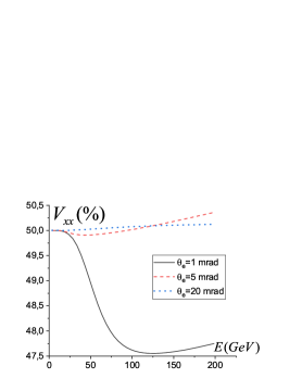
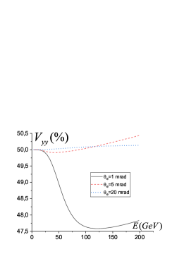
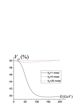
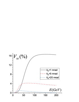
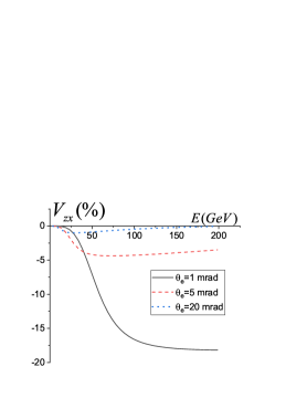
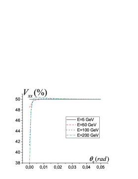
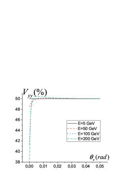
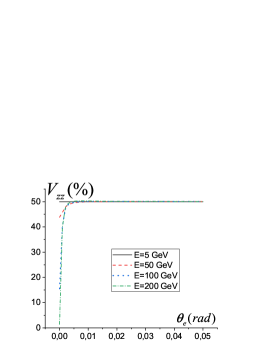
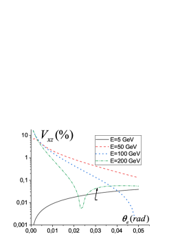
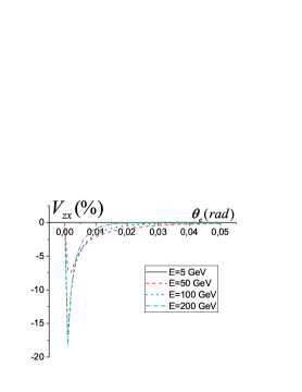
Figure 11: Polarization coefficients which describe the vector polarization transfer from the initial to the scattered deuteron in the reaction $\vec{d}\,^{V}+e\to\vec{d}\,^{V}+e$ given by Eqs. (73).

IV Discussion and conclusion

In this work we calculated the differential cross section and some polarization observables for the elastic reaction induced by deuteron scattering off electrons at rest assuming the one-photon-exchange approximation. We limited the study to the estimation of one-spin effects when one deuteron (initial or scattered) is tensor polarized, and to double-spin effects when two particles are vector polarized. In the last case, all possible polarization states are considered. Our analytical and numerical results are obtained under the condition that all components of the 3-vector polarization for every particle in reaction (1) are defined in the Lab system, as shown in Fig. 1. The same is required for the components of the deuteron tensor polarizations. In this respect, it should be noted that the combination of the form factors, included in $t_{20}$ and measured in $e-d$ scattering Abbott et al. (2000a), corresponds to the $z$-axis along the unit 3-vector of the momentum transfer Gakh and Merenkov (2004); Gakh et al. (2012) in the rest frame of the initial deuteron. Our choice corresponds to the direction opposite to the unit 3-vector of the initial electron 3-momentum (in Lab system, the $z$-axis is just along deuteron 3-momentum). Therefore $A_{zz}$ has the contribution of a term $~{}G_{M}\,G_{Q}$ which is absent in $t_{20}$. Along the numerical calculation we used the parametrization of the deuteron electromagnetic form factors suggested in Ref. Tomasi-Gustafsson et al. (2006) and extrapolate it to the small $Q^{2}$ region (Fig. 2). Others form factor parameterizations exhibit very similar behaviour in this region.

Our result can be applied to measure the polarization of or to create the polarization of the participating particles. Note, that the unpolarized cross section is large enough (see Fig. 3), indicating that the number of events in the different polarization conditions can be sufficient to perform fairly accurate measurements despite of the fact that the corresponding effects are at the percent level.

Our formalism is very general, based on the symmetries of the strong and electromagnetic interactions. The lepton and hadron tensors are obtained in terms of the deuteron electromagnetic current Eq. (11) and the density matrices of the initial and scattered deuteron, Eq.(̇18). All the coefficients, which describe the single- and double-spin effects, are the ratio of the corresponding spin-dependent parts of the matrix element squared by the spin-independent parts, i.e., $H_{\mu\nu}\,L^{\mu\nu}/(2\,{\cal D}).$ , according to the used normalization of the unpolarized cross section (see Eq. (26)). The additional factor 1/2 in the differential cross sections when the recoil electron polarization is measured (see Eqs. (49), (65),  (67)), is due to the density matrix of the recoil electron. Our main results are illustrated in Figs. (4-10) in which we plotted different coefficients as a function of the electron scattering angle $\theta_{e}$ at fixed values of the deuteron beam energy $E$ and vice versa.

In the Lab system the tensor asymmetries $A_{ij}$ (Fig. 4) and the tensor polarization coefficients $P_{ij}$ (Fig. 5) are small, not exceeding the order of percent. Nevertheless this situation leaves room for measurements due to large cross section. The coefficients of the polarization transfer $t_{ij}$ (Fig. 6) from the target to the recoil electron vary in the range $-1$ to $+1,$ which makes it possible to change the polarization of electrons. The coefficients $C_{ij}$ except $C_{xz}$ (Fig. 7) are on the level a few tens, thus the correlation between the vector polarizations of the deuteron beam and the target electrons is large and measurable.

The possibility to create vector polarized deuterons from polarized target electrons is illustrated by the polarization transfer coefficients $T_{ij}$ (Fig. 8). They are of the order of 10%, except $T_{xz}$, showing a realistic possibility of applications. The correlation between the vector polarization of the final deuterons and electrons is noticeable although not as large as for the initial ones (Fig. 9). It is quite unexpected that the vector polarization transfer coefficients $\widetilde{T}_{ij}$ (Fig. 10) from the initial deuterons to the recoil electrons is several times larger than $T_{ij}.$ The large values of the coefficients $V_{ij}$, which describe the vector polarization transfer from the initial o the scattered deuterons (Fig. 11) should also be noted.

Our formalism, being very general, gives the essential formulas for deuteron polariation and polarimetry studies. The specific ingredients of the deuteron structure are contained in the form factors. The sensitivity to different models is expected not to be large, because of the low-$Q^{2}$ involved and the constrains for static deuteron properties at $Q^{2}\to 0$.

V Acknowledgments

This work was partly supported (G.I.G, M.I.K. and N.P.M.) by the National Academy of Sciences via the program ”Participation in the international projects in high energy and nuclear physics” (project no.0121U111693).

References

- Adylov et al. (1974) G. Adylov et al., High energy physics. Proceedings, 17th International Conference, ICHEP 1974, London, England, July 01-July 10, 1974, Phys. Lett. B51, 402 (1974).
- Dally et al. (1977) E. B. Dally et al., Phys. Rev. Lett. 39, 1176 (1977).
- Dally et al. (1982) E. B. Dally et al., Phys. Rev. Lett. 48, 375 (1982).
- Dally et al. (1980) E. B. Dally et al., Phys. Rev. Lett. 45, 232 (1980).
- Amendolia et al. (1986) S. R. Amendolia et al. (NA7), Proceedings, 23RD International Conference on High Energy Physics, JULY 16-23, 1986, Berkeley, CA, Nucl. Phys. B277, 168 (1986).
- Amendolia et al. (1984) S. R. Amendolia et al., Phys. Lett. B146, 116 (1984).
- Abbiendi et al. (2016) G. Abbiendi et al., (2016), arXiv:1609.08987 [hep-ex] .
- Gakh et al. (2011) G. Gakh, A. Dbeyssi, D. Marchand, E. Tomasi-Gustafsson, and V. Bytev, Phys.Rev. C84, 015212 (2011), arXiv:1103.2540 [nucl-th] .
- Pohl et al. (2010) R. Pohl, A. Antognini, F. Nez, F. D. Amaro, F. Biraben, et al., Nature 466, 213 (2010).
- Bernauer et al. (2010) J. Bernauer et al. (A1 Collaboration), Phys.Rev.Lett. 105, 242001 (2010), arXiv:1007.5076 [nucl-ex] .
- Mohr et al. (2012) P. J. Mohr, B. N. Taylor, and D. B. Newell, Rev. Mod. Phys. 84, 1527 (2012).
- Gasparian (2014) A. Gasparian (PRad at JLab), Proceedings, 13th International Conference on Meson-Nucleon Physics and the Structure of the Nucleon (MENU 2013): Rome, Italy, September 30-October 4, 2013, EPJ Web Conf. 73, 07006 (2014).
- Cline et al. (2021) E. Cline, J. Bernauer, E. J. Downie, and R. Gilman, SciPost Phys. Proc. 5, 023 (2021).
- Xiong et al. (2019) W. Xiong et al., Nature 575, 147 (2019).
- Tiesinga et al. (2021) E. Tiesinga, P. J. Mohr, D. B. Newell, and B. N. Taylor, Rev. Mod. Phys. 93, 025010 (2021).
- Sick and Trautmann (1998) I. Sick and D. Trautmann, Nucl. Phys. A 637, 559 (1998).
- Antognini et al. (2021) A. Antognini, F. Kottmann, and R. Pohl, SciPost Phys. Proc. , 021 (2021).
- Pacetti and Gustafsson (2016) S. Pacetti and E. T. Gustafsson, to appear in Phys. Rev. C (2016), arXiv:1604.02421 [nucl-th] .
- Pacetti and Tomasi-Gustafsson (2020) S. Pacetti and E. Tomasi-Gustafsson, Eur. Phys. J. A 56, 74 (2020), arXiv:1812.04444 [nucl-th] .
- Glavanakov et al. (1996) I. V. Glavanakov, Yu. F. Krechetov, A. P. Potylitsyn, G. M. Radutsky, A. N. Tabachenko, and S. B. Nurushev, Nucl. Instrum. Meth. A381, 275 (1996).
- Reifarth and Litvinov (2014) R. Reifarth and Y. A. Litvinov, Phys. Rev. ST Accel. Beams 17, 014701 (2014), arXiv:1312.3714 [nucl-ex] .
- Taggart et al. (2019) M. P. Taggart et al., Phys. Lett. B 798, 134894 (2019), arXiv:1910.00870 [nucl-ex] .
- Williams et al. (2020) M. Williams et al., Phys. Rev. C 102, 035801 (2020), arXiv:1910.01698 [nucl-ex] .
- Phuc et al. (2019) N. T. T. Phuc, K. Yoshida, and K. Ogata, Phys. Rev. C 100, 064604 (2019), arXiv:1908.00667 [nucl-th] .
- Holl et al. (2019) M. Holl et al. (R3B), Phys. Lett. B 795, 682 (2019).
- A.I. and Rekalo (1977) A.I. and M. Rekalo, Hadron Electrodynamics(in russian) (Naukova Dumka, Kiev, 1977).
- Mohr and Taylor (2000) P. J. Mohr and B. N. Taylor, Rev. Mod. Phys. 72, 351 (2000).
- Ericson and Rosa-Clot (1983) T. E. O. Ericson and M. Rosa-Clot, Nucl. Phys. A 405, 497 (1983).
- Gourdin and C.A. (1964) M. Gourdin and P. C.A., Nuovo Cim. 32, 1137 (1964).
- Schildknecht (1964) D. Schildknecht, Physics Letters 10, 254 (1964).
- Ferro-Luzzi et al. (1998) M. Ferro-Luzzi et al., Nucl. Phys. A 631, 190C (1998).
- Dmitriev et al. (1985) V. F. Dmitriev, D. M. Nikolenko, S. G. Popov, I. A. Rachek, Y. M. Shatunov, D. K. Toporkov, E. P. Tsentalovich, Y. G. Ukraintsev, B. B. Voitsekhovsky, and V. G. Zelevinsky, Phys. Lett. B 157, 143 (1985).
- Gilman et al. (1990) R. A. Gilman et al., Phys. Rev. Lett. 65, 1733 (1990).
- Ferro-Luzzi et al. (1996) M. Ferro-Luzzi et al., Phys. Rev. Lett. 77, 2630 (1996).
- Bouwhuis et al. (1999) M. Bouwhuis, R. Alarcon, T. Botto, J. F. J. van den Brand, H. J. Bulten, S. Dolfini, R. Ent, M. Ferro-Luzzi, D. W. Higinbotham, C. W. de Jager, J. Lang, D. J. J. de Lange, N. Papadakis, I. Passchier, H. R. Poolman, E. Six, J. J. M. Steijger, N. Vodinas, H. de Vries, and Z.-L. Zhou, Phys. Rev. Lett. 82, 3755 (1999).
- Nikolenko et al. (2003a) D. M. Nikolenko et al., Phys. Rev. Lett. 90, 072501 (2003a).
- Nikolenko et al. (2003b) D. M. Nikolenko et al., Nucl. Phys. A 721, C409 (2003b).
- Schulze et al. (1984) M. E. Schulze et al., Phys. Rev. Lett. 52, 597 (1984).
- Garcon et al. (1994) M. Garcon et al., Phys. Rev. C 49, 2516 (1994).
- Abbott et al. (2000a) D. Abbott et al. (JLAB t(20)), Phys. Rev. Lett. 84, 5053 (2000a), arXiv:nucl-ex/0001006 .
- Haftel et al. (1980) M. I. Haftel, L. Mathelitsch, and H. F. K. Zingl, Phys. Rev. C 22, 1285 (1980).
- Alexa et al. (1999) L. C. Alexa et al. (Jefferson Lab Hall A), Phys. Rev. Lett. 82, 1374 (1999), arXiv:nucl-ex/9812002 .
- Bosted et al. (1990) P. E. Bosted et al., Phys. Rev. C 42, 38 (1990).
- Abbott et al. (2000b) D. Abbott et al. (JLAB t20), Eur. Phys. J. A 7, 421 (2000b), arXiv:nucl-ex/0002003 .
- Kobushkin and Syamtomov (1995) A. P. Kobushkin and A. I. Syamtomov, Phys. Atom. Nucl. 58, 1477 (1995), arXiv:hep-ph/9409411 .
- Iachello et al. (1973) F. Iachello, A. D. Jackson, and A. Lande, Phys. Lett. B 43, 191 (1973).
- Bijker and Iachello (2004) R. Bijker and F. Iachello, Phys. Rev. C 69, 068201 (2004), arXiv:nucl-th/0405028 .
- Tomasi-Gustafsson et al. (2006) E. Tomasi-Gustafsson, G. I. Gakh, and C. Adamuscin, Phys. Rev. C 73, 045204 (2006), arXiv:nucl-th/0512039 .
- Gakh and Merenkov (2004) G. I. Gakh and N. P. Merenkov, J. Exp. Theor. Phys. 98, 853 (2004).
- Gakh et al. (2012) G. I. Gakh, M. I. Konchatnij, and N. P. Merenkov, J. Exp. Theor. Phys. 115, 212 (2012), arXiv:1202.2225 [hep-ph] .