Fourier Analysis of Signals on Directed Acyclic Graphs (DAG)
Using Graph Zero-Padding

Abstract

Directed acyclic graphs (DAGs) are used for modeling causal relationships, dependencies, and flows in various systems. However, spectral analysis becomes impractical in this setting because the eigendecomposition of the adjacency matrix yields all eigenvalues equal to zero. This inherent property of DAGs results in an inability to differentiate between frequency components of signals on such graphs. This problem can be addressed by alternating the Fourier basis or adding edges in a DAG. However, these approaches change the physics of the considered problem. To address this limitation, we propose a graph zero-padding approach. This approach involves augmenting the original DAG with additional vertices that are connected to the existing structure. The added vertices are characterized by signal values set to zero. The proposed technique enables the spectral evaluation of system outputs on DAGs (in almost all cases), that is the computation of vertex-domain convolution without the adverse effects of aliasing due to changes in a graph structure, with the ultimate goal of preserving the output of the system on a graph as if the changes in the graph structure were not done.

1 Introduction

Graph signal processing is an emerging research area at the intersection between signal processing and graph theory, dealing with the analysis, processing, and interpretation of data defined on graphs [1, 2, 3, 4, 5, 6, 7, 8]. In many real-world applications, either the domain of the data or the data structure itself can be represented by graphs, with edges representing relationships or interactions among data [6, 8].

One particular type of graph that is of great significance in various domains is the Directed Acyclic Graph (DAG) [9, 10, 11, 12, 13, 15]. DAG is a special type of directed graph, without cycles. DAGs are commonly used to model causal relationships, dependencies, and flows in various systems [9]. In this context, DAGs are used to model and analyze dynamic systems where information (or signal) flows from one vertex to another, causing a cascade of effects. This is particularly relevant in fields, like epidemiology, finance, neuroscience, and machine learning, where understanding the causal relationships between variables or events can lead to better predictions and interventions [9, 13, 14].

Spectral analysis and processing based on the standard Graph Fourier Transform (GFT) is impossible for signals on DAGs, since all eigenvalues of the adjacency matrix are equal to zero, meaning that the frequency components of the analyzed signal cannot be distinguished [9].

The majority of endeavors aimed at resolving this issue, concentrate on altering the Fourier basis for Jordan normal form computation, which can significantly influence the graph signal processing methods [16, 17, 18, 19, 20, 21, 22, 23, 24]. To tackle the spectral analysis issue, while preserving the integrity of the Fourier basis, an algorithm has recently been proposed in [25]. The core concept entails strategically adding optimal edges to the graph until all non-trivial Jordan blocks are illuminated. This approach inherently changes the physics of the graph signal processing problem and the output of a system on this graph. It is also important to emphasize that in practical scenarios, the identification of suitable edges is contingent upon having access to the Jordan normal form of the adjacency matrix.

In this paper, inspired by the zero-padding in classical signal processing, we present a new concept of graph zero-padding which is implemented by adding vertices connected to the existing graph structure, with the corresponding signal values equal to zero. This model leads to the possibility to calculate the output of a graph system (filtering based on convolution), without aliasing effects (keeping the original DAG output as if the changes in the graph structure were not done). The proposed concept, along with the idea of forming a Hamiltonian path in a general DAG, is used to define a simple algorithm that can simultaneously eliminate the Jordan block associated to the eigenvalue zero. Indeed, through the implementation of this algorithm, all eigenvalues of the adjacency matrix of the zero-padded graph are non-zero. In the vast majority of situations, these eigenvalues will be distinct, indicating the achievement of diagonalizability, with only a few rare exceptions, that require further attention. Diagonalizability of the adjacency matrix allows GFT analysis and application of various spectral tools on the considered graph [26]. A simple interpretation of the speed of change (discrete frequency) in the GFT basis of a DAG, is also introduced using the eigenvector phases, as an alternative to the common total variation factor. The basic idea for the proposed concept was introduced in a special case of connected DAGs in [27]. The concept of graph zero-padding presented in this paper is general and could be used on any graph.

The paper is organized as follows. In Section 2, the basic theory regarding graphs, signals on a graph, systems on a graph, and GFT is presented. Next, in Section 3 we present some fundamental properties of DAGs. Classical signal processing in a graph framework is presented in Section 4. In Section 5 we present graph zero-padding on a special case of connected DAG. General DAG zero-padding is presented in Section 6. Section 7 concludes the paper. The proposed approach is illustrated on numerical examples.

2 Graph Signal Processing

Consider a graph $\mathcal{G}=(\mathcal{V},\mathcal{E})$ consisting of a finite set $\mathcal{V}$ of $N$ vertices, and set $\mathcal{E}\subset\mathcal{V}\times\mathcal{V}$ of edges, connecting the vertices, and reflecting their mutual relations. The graph can be modeled by adjacency matrix $\mathbf{A}$. The elements $a_{mn}$ of this matrix have value $1$ if an edge between vertex $m$ and vertex $n$ exists, and value $0$ if such edge does not exist.

A signal on a graph is defined as $N$-dimensional vector

$$\mathbf{x}=\begin{bmatrix}x(1)&x(2)&\ldots&x(N)\end{bmatrix}^{T},$$ (1)

where signal value $x(n)$ is associated to $n$-th vertex of the considered graph.

Graph shift operator is a matrix $\mathbf{T}$ that convert given graph signal $\mathbf{x}$ into its shifted version $\mathbf{y}$,

$$\mathbf{y}=\mathbf{T}\mathbf{x}.$$

The simplest and most commonly used shift operator on directed graphs is the adjacency matrix $\mathbf{T}=\mathbf{A}$. That kind of shift is called a “backward shift”.

A linear system on a graph is defined as a linear combination of the signal and its shifted versions. System output can be calculated as

$$\mathbf{y}=h_{0}\mathbf{x}+h_{1}\mathbf{T}\mathbf{x}+h_{2}\mathbf{T}^{2}\mathbf{x}+\cdots+h_{M}\mathbf{T}^{M}\mathbf{x},$$ (2)

where $M$ is the system order and $h_{m}$, $m=0,1,\ldots,M$ are the system coefficients, corresponding to the classical impulse response [5, 6, 7].

Note that every system on a given graph can be determined with $M<N$ coefficients due to the fact that arbitrary matrix power $\mathbf{T}^{n}$ can be expressed as a linear combination of matrix powers $\mathbf{T}^{m}$, $m=0,1,\ldots,N-1$.

Fourier transform on directed graphs is defined with the assumption that the adjacency matrix is diagonalizable, meaning that there exists an invertible matrix $\mathbf{V}$ and a diagonal matrix $\mathbf{\Lambda}$ such that

$$\mathbf{A}=\mathbf{V}^{-1}\mathbf{\Lambda}\mathbf{V}.$$

The diagonal elements of matrix $\mathbf{\Lambda}$ are eigenvalues, $\lambda_{k}$, $k=1,2,\dots,N$, of the adjacency matrix $\mathbf{A}$ and the columns of $\mathbf{V}$ are the corresponding eigenvectors, $\mathbf{v}_{k}$, $k=1,2,\dots,N$. The GFT of a signal, $x(n)$, on vertices $n=1,2,\dots,N$, is defined as

$$X(k)=\sum_{n=1}^{N}x(n)u_{k}(n).$$ (3)

Here, $u_{k}(n)$ represents the value of the $k$th column of matrix $\mathbf{V}^{-1}$, corresponding to the vertex $n$. The matrix form of the GFT reads $\mathbf{X}=\mathbf{V}^{-1}\mathbf{x}$. The inverse graph Fourier transform (IGFT) is defined by

$$x(n)=\sum_{k=1}^{N}X(k)v_{k}(n),$$ (4)

or, in a matrix form $\mathbf{x}=\mathbf{V}\mathbf{X}$. Here, $v_{k}(n)$ is the value of the $k$th eigenvector (column of matrix $\mathbf{V}$), corresponding to the vertex $n$.

The system on a graph can be written using the GFTs of the input and output signal as [6]

$$\mathbf{Y} =\big{(}h_{0}\mathbf{I}+h_{1}\boldsymbol{\Lambda}+h_{2}\boldsymbol{\Lambda}^{2}+\cdots+h_{M}\boldsymbol{\Lambda}^{M}\Big{)}\mathbf{X},\ \ \mathrm{or}$$

$$\mathbf{Y} =\mathbf{H}(\boldsymbol{\Lambda})\mathbf{X},$$ (5)

where $\mathbf{H}(\boldsymbol{\Lambda})$ is the system transfer function.

3 DAG

In many cases of practical interest, especially for DAGs, the adjacency matrix is not diagonalizable and the Fourier analysis cannot be performed without graph modifications. Two examples of a DAG with $N=7$ vertices are presented in Fig. 1. The graph on the left side is not connected and the graph on the right side is connected.

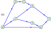
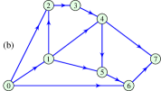
Figure 1: Examples of a directed acyclic graph (DAG): (a) Nonconnected DAG (for example, path connecting vertices 1 and 2 does not exist), (b) Connected DAG (there exist a path between any pair of vertices).

Every DAG induces partial ordering on a vertex set. If vertex numbering follows this partial ordering then the adjacency matrix will be an upper triangular matrix, with zeros on the main diagonal (since loops are not allowed in acyclic graphs). Specifically, if DAG is connected, we have the total ordering and a unique numbering of graph vertices that correspond to a Hamiltonian path in the connected DAG, as shown in Fig. 1(b).

Remark: Adjacency matrix of a DAG is nilpotent with nilpotency index smaller than $N$. All eigenvalues of DAG adjacency matrix are equal to 0.

If the adjacency matrix, $\mathbf{A}$, is used as a shift operator on DAGs then any system on a DAG can be written in a form

$$\mathbf{y}=h_{0}\mathbf{x}+h_{1}\mathbf{A}\mathbf{x}+h_{2}\mathbf{A}^{2}\mathbf{x}+\cdots+h_{M}\mathbf{A}^{M}\mathbf{x},$$ (6)

where $M+1$ is the nilpotency index of $\mathbf{A}$.

4 Classical Zero-padding within the Graph Framework

If we have a classical signal in the discrete-time domain, $x(n)$, of length $N$, then its domain can be presented in the form of a directed path graph with $N$ vertices, as shown in Fig. 2(a).

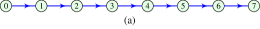
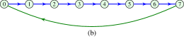
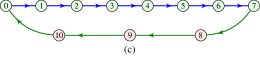
Figure 2: (a) Domain of a classical discrete-time signal of length $N=8$, (b) Domain of the classical signal as it is inherently used in the DFT calculation with $N=8$, (c) Domain of the zero-padded classical signal as it must be used in the DFT based calculation for the output of a FIR system whose order is $M\leq 3$, with $N=8$.

Remark: It is well known that for the calculation of the discrete Fourier transform (DFT) of this signal we must assume signal periodicity. In graph terminology, it means that we have to make the graph domain of the signal circular. The minimum number of samples for the DFT calculation of the assumed signal is $N$, meaning that we inherently add one edge connecting the last and the first vertex, see Fig. 2(b).

This necessary and obvious domain modification can be interpreted and justified within the graph terminology as well. The adjacency matrix, $\mathbf{A}$, of the path graph from Fig. 2(a) is a super-diagonal matrix

$$\small\mathbf{A}=\begin{bmatrix}0&1&0&0&0&0&0&0\\ 0&0&1&0&0&0&0&0\\ 0&0&0&1&0&0&0&0\\ 0&0&0&0&1&0&0&0\\ 0&0&0&0&0&1&0&0\\ 0&0&0&0&0&0&1&0\\ 0&0&0&0&0&0&0&1\\ 0&0&0&0&0&0&0&0\\ \end{bmatrix},$$

with all eigenvalues following from $\mathrm{det}\big{(}\mathbf{A}-\lambda\mathbf{I}\big{)}=0$, being

$$\lambda_{k}=0,\ \text{ for }\ k=0,1,\dots,N-1.$$

This adjacency matrix $\mathbf{A}$ is not diagonalizable and the Fourier analysis on this graph, as the signal domain, is not possible (note that if we assume an undirected graph, as the signal domain, then the Fourier analysis would be possible, but that changes the physics of the problem).

Diagonalization by making the domain circular. If we make the domain circular, by adding one edge from the last (sink) vertex to the first (source) vertex, we get the adjacency matrix

$$\small\mathbf{A}_{C}=\begin{bmatrix}0&1&0&0&0&0&0&0\\ 0&0&1&0&0&0&0&0\\ 0&0&0&1&0&0&0&0\\ 0&0&0&0&1&0&0&0\\ 0&0&0&0&0&1&0&0\\ 0&0&0&0&0&0&1&0\\ 0&0&0&0&0&0&0&1\\ 1&0&0&0&0&0&0&0\\ \end{bmatrix}.$$ (7)

This matrix is obviously diagonizable. Eigenvalues of matrix $\mathbf{A}_{C}$, of size $N\times N$, are obtained as the solutions of

$$\lambda^{N}=1.$$

They are all distinct and equal to

$$\lambda_{k}=e^{j\frac{2\pi}{N}k},\quad k=0,1,\ldots,N-1,$$

where $k$ is the frequency index.

Frequency interpretation. For $0\leq k<\frac{N}{2}$ we talk about “positive” frequencies, while indices $\frac{N}{2}\leq k<N$ are associated to “negative” frequencies. Therefore, the graph spectral analysis on a circular graph coincides with the classical DFT analysis. Note that the discrete frequency $\omega_{k}=\frac{2\pi}{N}k$ can be obtained as an angle of the corresponding eigenvalue $\lambda_{k}$, that is,

$$\omega_{k}=\arg\{\lambda_{k}\}.$$

Frequency is used to measure the speed of change in the eigenvectors in classical DFT. Another way to measure the changes in the eigenvectors (GFT basis) is in using the total variation [6, 15]

$$E_{TV}(k)=\Big{|}1-\frac{\lambda_{k}}{\max_{m}(\lambda_{m})}\Big{|}^{2}.$$

This parameter is used in graph signal processing to sort the eigenvectors from low to high frequency.

Signal processing and zero-padding. Assume now that we want to process the considered classical signal $x(n)$ by a general FIR system whose impulse response $h_{n}$ is of the length $(M+1)$, that is by a system of order $M$. This classical system is defined within the graph framework by (2). Its discrete-time domain realization can be written as

$$y(n)=h_{0}x(n)+h_{1}x(n-1)+\dots+h_{M-1}x(n-M).$$

If we want to use the DFT to calculate the output (which is almost a standard routine in the DSP processors), then we must zero-pad the original signal by at least $M$ zeros before the DFT is applied. After zero-padding, the DFT will produce the output that corresponds to the original non-periodic output signal that is shown in Fig. 3.

Within the graph terminology, the zero-padding of the original signal (before we make it periodic) means that we must add at least $M$ vertices in the backward path from the sink to the source vertex, as illustrated in Fig. 4. The adjacency matrix of the zero-padded graph is of the same form as in (7), but of order $N+M$. It is diagonalizable with all distinct eigenvalues

$$\lambda_{k}=e^{j\frac{2\pi}{N+M}k},\quad k=0,1,\ldots,N+M-1,$$

and corresponds to the DFT analysis of a signal with $N+M$ samples, after zero-padding.

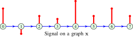
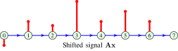
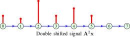
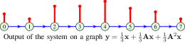
Figure 3: Signal $x(n)$ of length $N=8$ on a graph as its domain along with its shifted versions. The last subplot is the output of a system on a graph of order $M=2$ with system coefficients equal to $1/3$.

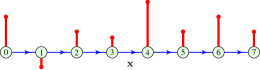
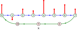
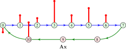
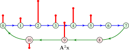
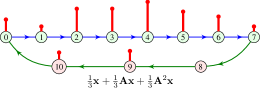
Figure 4: (a) Signal $x(n)$ of length $N=8$ on a graph as its domain. (b) Signal on a graph as it must be used in the DFT output calculation on a FIR system whose order is $M\leq 3$. (c) Signal $x(n-1)$ shifted on a graph from (b). (d) Signal $x(n-2)$ on a graph from (b). (e) Output signal as a circular (DFT) convolution $\mathbf{y}=\mathbf{x}*[\frac{1}{3},\frac{1}{3},\frac{1}{3}]$ equal (within the basic period) to the aperiodic convolution of the same signal and system.

5 Connected DAG Zero-Padding

Connected DAG has one source vertex and one sink vertex. Moreover, there exists a path from sink to source traversing every vertex in a DAG (Hamiltonian path).

From the previous section, we can conclude that a possible solution for a non-diagonalizable adjacency matrix is to add an edge from the sink to the source vertex in order to obtain a new graph with a diagonalizable adjacency matrix. If we want to keep the same output of a graph filter (of an order less than or equal to $M$) on the original and a modified DAG, then instead of adding an edge we should add a path of length $M$ connecting the sink and the source in the original connected DAG.

With the described zero-padding, the shifts produced by $\mathbf{A}^{m}\mathbf{x}$, $m=0,1,2,\dots,M$ on the original graph, will correspond to the shifts on the zero-padded graph, while the shifted signal values, will be trapped in the added path from the sink to the source that is long enough so they do not influence the signal at the vertices that belong to original graph, during the system processing time.

The adjacency matrix of the zero-padded graph can be presented in a block form as

$$\mathbf{A}_{ZP}=\begin{bmatrix}\mathbf{A}&\mathbf{C}\\ \mathbf{D}&\mathbf{J}\end{bmatrix},$$ (8)

where $\mathbf{A}$ is $N\times N$ adjacency matrix of the connected DAG, $\mathbf{J}$ is a matrix of size $M\times M$, with ones at super-diagonal and zeros elsewhere. Matrix $\mathbf{C}$ is of size $N\times M$, with all zeros except the lower left corner where it has value 1. This block represents the connection of the DAG sink to the first vertex of the added path graph. Matrix $\mathbf{D}$ is of size $M\times N$ with all zeros except the lower left corner where it has value 1. This block represents the edge from the last vertex of the added path graph to the source of DAG.

Determinant in the zero-padded graph: It is easy to check that determinant of $\mathbf{A}_{ZP}$ is non-zero, in specific its value is either 1 or $-1$.

To illustrate the proposed concept, consider a connected DAG with 8 vertices (Fig. 1(b)), with an adjacency matrix

$$\small\mathbf{A}=\begin{bmatrix}0&1&1&0&0&0&1&0\\ 0&0&1&0&1&1&0&0\\ 0&0&0&1&0&0&0&0\\ 0&0&0&0&1&0&0&0\\ 0&0&0&0&0&1&0&1\\ 0&0&0&0&0&0&1&0\\ 0&0&0&0&0&0&0&1\\ 0&0&0&0&0&0&0&0\end{bmatrix}.$$

For zero-padding with $M=2$ additional vertices, the matrix $\mathbf{A}_{ZP}$ has the following form

$$\small\mathbf{A}_{ZP}=\left[\begin{array}[]{cccccccc|cc}0&1&1&0&0&0&1&0&0&0\\ 0&0&1&0&1&1&0&0&0&0\\ 0&0&0&1&0&0&0&0&0&0\\ 0&0&0&0&1&0&0&0&0&0\\ 0&0&0&0&0&1&0&1&0&0\\ 0&0&0&0&0&0&1&0&0&0\\ 0&0&0&0&0&0&0&1&0&0\\ 0&0&0&0&0&0&0&0&1&0\\ \hline\cr 0&0&0&0&0&0&0&0&0&1\\ 1&0&0&0&0&0&0&0&0&0\end{array}\right],$$

and we obtain a zero-padded graph presented in Fig. 5. This adjacency matrix is now diagonizable and a system on this DAG can be analyzed and implemented in the spectral domain.

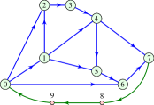
Figure 5: Example of DAG from Fig. 1 (b) with additional vertices (marked with red) and edges (green) needed for GFT analysis.

5.1 Numeric Examples

Five examples of zero-padded connected DAGs are presented in Fig. 6. The first case is the most simple one, that is the path graph. This graph transforms into a cycle graph after the zero-padding (here we use zero-padding with $M=2$) and the classical Fourier analysis follows from the eigendecomposition of the adjacency matrix. Eigenvalues lie equally spaced on the unit circle as shown in Fig. 6.

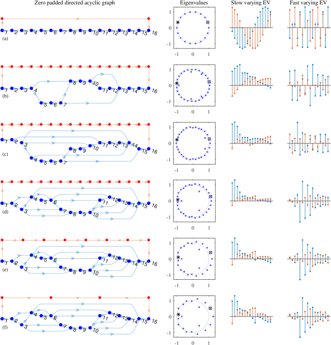
Figure 6: Examples of zero-padded connected DAG. Simple path graph (a) zero-padded with $M=2$ vertices; connected DAG with 3, 5, and 10 additional edges compared to path graph zero-padded with $M=16$ vertices (b-d); same DAG as in (d) zero-padded with $M=8$ and $M=4$ (e,f). Original DAGs are presented with blue vertices and edges. Nodes and edges added by zero-padding are in red. For each zero-padded graph eigenvalues are presented. Two eigenvectors that correspond to a low and a high-frequency eigenvalue are also presented (real parts in blue and imaginary parts in red). Corresponding eigenvalues are marked by a square (low-frequency) and a star (high-frequency) on the eigenvalues plot.

In more complex DAG examples (Fig. 6 (b,c,d)) we add more edges to the path graph in order to keep the connectivity and avoid cycles. Here, we present graphs with 3, 5, and 10 additional edges. In all presented cases, we can see from Fig. 6 that the eigenvalues lie close to the unit circle, with nonuniform, but almost equal spacing. Here, graph zero-padding with $M=N=16$ is used. Finally in Fig. 6 (e,f), the same DAG as in Fig. 6 (d) is zero-padded with $M=8$ and $M=4$ vertices. Using zero-padding with $M<N$ guarantees equality of the output calculated in the vertex domain and output calculated using the spectral domain for systems of order up to $M$.

For each considered graph in Fig. 6, two eigenvectors are presented on the right. Since eigenvectors are complex, we present their real part in blue and the imaginary part in red. We choose one slow-varying eigenvector that corresponds to a low frequency (marked by a square in the eigenvalue plot in Fig. 6) and one fast-varying eigenvector with the corresponding eigenvalue marked by a star. From these plots, we can observe that the concept of slow-varying and fast-varying Fourier basis functions (eigenvectors), inherently obvious in the classical Fourier domain (circular graph), can be straightforwardly generalized to more complex directed graphs.

6 General DAG zero-padding

For a general DAG, we should consider adding more than one edge (path if we want to apply zero-padding) to the original DAG in order to make the adjacency matrix of a new graph diagonalizable, with all non-zero eigenvalues, that will be appropriate for performing the GFT analysis. How to add a minimal number of edges in order to make the adjacency matrix diagonalizable is not an easy task. It can be solved using a combinatorial approach (exhaustive search), but only for a small graph size $N$. Another recently proposed approach uses matrix perturbation theory [25]. Here we will propose a simple and fast but sub-optimal strategy. It is based on two steps:

• First we add a sufficient number of edges in order to make the DAG connected. We can use the procedure described in Algorithm 1.

• We add an edge connecting sink and source of the connected DAG, obtained in the previous step.

If we renumber vertices in the connected DAG according to their position in the Hamiltonian path, the adjacency matrix becomes upper triangular with ones on the super-diagonal. Adding vertices in the return path with an appropriate numbering ($\text{sink}+1,\text{sink}+2,\ldots$) keeps ones at the adjacency matrix super-diagonal and adds 1 into its lower left corner.

Algorithm 1 Make a DAG connected

directed acyclic graph $\mathcal{G}$

connected directed acyclic graph $\mathcal{G}_{2}$

$\mathcal{G}_{1}\leftarrow\mathcal{G}$

$\mathcal{G}_{2}\leftarrow\mathcal{G}$

while $\mathcal{G}_{1}$ is not empty do

     $s\leftarrow$ list of all sources in $\mathcal{G}_{1}$

     if there is more than one source in $s$ then

         connect sources $s$ by path in $\mathcal{G}_{2}$

     end if

     remove sources $s$ from $\mathcal{G}_{1}$

end while

$h\leftarrow$ Hamiltonian path in $\mathcal{G}_{2}$

remove all edges from $\mathcal{G}_{2}$ that are not in $\mathcal{G}$ and does not belong to $h$

return $\mathcal{G}_{2}$

	Total DAGs	Diagonal.	Algeb. Mult.$\mathrm{}>1$
$N=7$	$32,768$	$32,250$	$518$	$1.58\%$
$N=7$ (1-ZP)	$32,768$	$32,758$	$10$	$0.03\%$
$N=8$	$2,097,152$	$2,075,682$	$21,470$	$1.02\%$
$N=8$ (1-ZP)	$2,097,152$	$2,088,106$	$9,046$	$0.43\%$
$N=8$ (2-ZP)	$2,097,152$	$2,095,224$	$1,928$	$0.09\%$

Table 1: The total number of connected DAGs for $N=7$ and $N=8$ vertices ("Total DAGs" column), along with the number of DAGs, among them, whose eigenvalues of the adjacency matrix are all distinct ("Diagonal." column) after adding sink-to-source edge, and the number of such DAGs with an algebraic multiplicity of the adjacency matrix greater than one ("Algeb.Mult.>1" column) for at least one eigenvalue (possibly nondiagonalizable). (1-ZP) means that the added sink-to-source edge in DAG is zero-padded with one vertex, while (2-ZP) means that two vertices are added in this edge/path.

Invertibility, Diagonalizability, and Algorithm’s Efficacy. After Algorithm 1 is executed, the adjacency matrix attains full rank, indicating that it becomes invertible. This property implies that all eigenvalues of the considered matrix are non-zero. However, the invertibility does not guarantee diagonalizability. The nondiagonalizability of the adjacency matrix of a graph obtained after Algorithm 1 is a very rare event. Even in these rare cases, after the added edges are zero-padded, it often happens that the resulting adjacency matrix becomes diagonalizable.

For relatively small graphs, with $N=7$ and $N=8$, it is possible to construct all possible connected DAGs, with added sink-to-source connection (edge or path), and check the algebraic multiplicity of the eigenvalues, since all distinct eigenvalues are sufficient for the diagonalizability. By adding only sink-to-source edge to all considered DAGs the diagonalizability is achieved in 98,42% and 99% for $N=7$ and $N=8$, respectively. These results are presented in Table 1, rows one and three.

After one or two vertices are added in the sink-to-source path, we can see that the adjacency matrix diagonalizability is increased to above 99.6% cases (rows two, four, and five in Table 1).

It is very interesting that all 518 cases (out of 32768) that were not diagonalizable with $N=7$, become diagonalizable after adding one vertex in the sink-to-source path. However, 10 graphs that were diagonalizable after the sink-to-source edge is added, become nondiagonalizable after this vertex is added. We checked that in all 32768 possible connected DAGs with $N=7$, and in all 2097152 possible connected DAGs for $N=8$, the diagonalizability is achieved either with a single sink-to-source edge or with one added vertex in the sink-to-source path. Since the number of added vertices, could be changed, as far as their number is greater or equal to the order of a system on the graph, it means that in this way the diagonalizability can be achieved, in practically (almost) all cases.

6.1 Graph Zero-Padding from a Linear Algebraic Perspective

In the initial step, it becomes clear that the nilpotency of the adjacency matrix, with nilpotency index $P$ indicates that the geometrical multiplicity of the unique eigenvalue $0$ is equal to $P+1$ exactly. This, in turn, implies that in the Jordan normal form, there are precisely $P+1$ nontrivial Jordan blocks associated with the eigenvalue $0$. To achieve diagonalizability, there is no choice but to eliminate all of these blocks. Algorithm 1 addresses the task of consolidating all these non-trivial Jordan blocks into a single block while maintaining the acyclic nature of the graph.

After successfully constructing the Hamiltonian path, an extra edge is added to connect the sink to the source. This necessitates the application of a new perturbation, which is in the form of a rank-one elementary matrix. Empirical evidence confirms that, in almost all scenarios, diagonalizability is successfully achieved in this phase, especially after zero-padding and adding additional vertices.

In exceptional instances, the second perturbation may introduce a few nontrivial Jordan blocks, which can also be resolved by the inclusion of a small number of randomly positioned edges. Through these insightful observations and a careful examination of Algorithm 1 on graphs, significant progress can be achieved by addressing the challenges in the way discussed in the recent related work [25].

6.2 Examples

For the DAG presented in Fig 1(a), we should add two edges in order to the make DAG connected, for example, edges $(1,2)$ and $(4,5)$. These edges are shown in red color in Fig. 7. By adding the return edge $(7,0)$, indicated by the green color in Fig. 7, we obtain the graph where we can define the GFT.

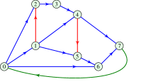
Figure 7: An example of DAG with additional edges needed for GFT analysis. Red edges are used to make the DAG connected with a Hamiltonian path 0-1-2-3-4-5-6-7, while the green edge is used for a sink-to-source edge, used to convert the Hamiltonian path to a Hamiltonian cycle.

If we want to keep the same behavior of the original DAG and the modified DAG for signal processing and systems on graphs of maximal order $M$, we should insert new paths in the graph with additional $M$ vertices, instead of each edge which is added in the previous procedure. For the DAG presented in Fig. 1(a), by using $M=2$ and introducing new vertices, the obtained zero-padded graph is presented in Fig. 8 (top).

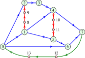
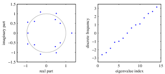
Figure 8: (top) An example of a zero-padded graph with additional vertices needed for achieving the same behavior of systems of order less than or equal to $M=2$ on the original DAG and the obtained zero-padded graph. (bottom) Eigenvalues of the zero-padded graph, with a relationship between the eigenvalue index and the corresponding discrete frequency.

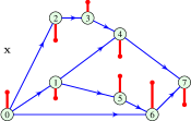
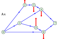
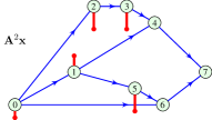
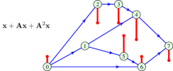
Figure 9: An example of signal processing using second order system on a DAG.

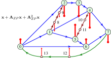
Figure 10: Signal processing on the DAG from Fig. 9, after zero-padding is done, so that the GFT can be used.

In the considered case we can add more than $M$ zero-padding vertices in added paths (sometimes $M$ is not known in advance). Having in mind that the adjacency matrix of the original DAG, presented in Fig. 1(a), has a nilpotency index of 5 meaning that any system on that graph is of order smaller than 5. By inserting $M=4$ vertices in each path, an arbitrary system defined on the original DAG and applied to the zero-padded DAG will produce the same output (when we neglect signal values at the vertices added through the zero-padding procedure).

As an example, consider a signal on the DAG presented in Fig. 9 (top). Shifted signals are presented in the same figure. Then we apply a system of the second order on this graph, defined by

$$\mathbf{y}=\mathbf{x}+\mathbf{A}\mathbf{x}+\mathbf{A}^{2}\mathbf{x}.$$

The output signal is shown in Fig. 9 (bottom).

The same signal and system are then used on a zero-padded DAG shown in Fig. 8 (top), assuming zero signal values at the added vertices ($8,9,\ldots,13$). The system output is presented in Fig. 10. The output signal at vertices ($0,1,\ldots,7$) is the same as in the case of the original DAG (see Fig. 9 (bottom)). Signal values at the vertices added to the original DAG by zero-padding procedure could be discarded.

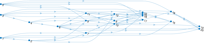
(a)

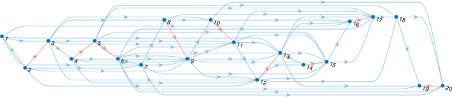
(b)

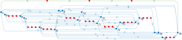
(c)

Figure 11: (a) Original DAG, (b) connected DAG with added edges marked by red color, (c) zero-padded DAG with added vertices ($M=3$) marked by red color and return path marked by green color.

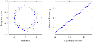
Figure 12: Eigenvalues of the zero-padded connected DAG shown in Fig. 11(c)

A more complex example is presented in Fig. 11 (a). Here we consider a DAG with $N=20$ vertices and 54 edges. There are three sources ($1,3$ and $5$) and two sinks ($19$ and $20$). This DAG is obviously not connected. Next, we add edges, according to the Algorithm 1, in order to make the DAG connected. Added edges are shown in red color in Fig. 11(b). Then, we perform zero-padding by replacing each added edge with a path graph with $M=3$ additional vertices, for each path, and adding a return path from the sink to the source, marked in green color in Fig. 11(c). Each vertex added by zero-padding is marked by red color. Eigenvalues of the obtained zero-padded graph are given in Fig. 12 (left). They are all distinct, ensuring the diagonalizability of the adjacency matrix. The relation between the eigenvalue index and the discrete frequency value, calculated as an angle of the corresponding eigenvalue is presented in Fig. 12 (right). It can be seen that this relation is close to the linear one. The signal processed on this zero-padded graph with a system of up to the third order would remain the same as in the original DAG, where the Fourier analysis was not possible.

Finally, we have generated a random signal $\mathbf{x}=\mathrm{rand}(20,1)$ on a graph given in Fig. 11(a). The graph and the signal are zero-padded according to the presented procedure (see Fig. 11(c)). Then the GFT of zero-padded signal $\mathbf{x}_{ZP}$ is calculated as $\mathbf{X}_{ZP}=\mathbf{V}^{-1}\mathbf{x}_{ZP}$. The obtained GFT is multiplied by the system transfer function

$$\mathbf{H}(\mathbf{\Lambda})=h_{0}\mathbf{I}+h_{1}\mathbf{\Lambda}+h_{2}\mathbf{\Lambda}^{2}+h_{3}\mathbf{\Lambda}^{3}$$

in order to obtain GFT of the output signal $\mathbf{Y}_{ZP}=\mathbf{H}(\mathbf{\Lambda})\mathbf{X}_{ZP}$. The output signal is calculated by IGFT as $\mathbf{y}_{ZP}=\mathbf{V}\mathbf{Y}_{ZP}$. Its values on the vertices from the original DAG are the same as the ones obtained by a direct calculation in the vertex domain.

7 Conclusion

Here, we have proposed a graph zero-padding concept in order to overcome the inherent limitations associated with spectral signal analysis and processing on DAGs. The main idea is motivated by classical zero-padding and its graph framework interpretation. In the case of a connected DAG, the extension is straightforward by adding a single backward path (or edge) whose length is equal to the maximum order of the system used for graph signal processing. The determinant of the adjacency matrix of the zero-padded graph is either 1 or $-1$ meaning that all eigenvalues are now nonzero. For a general form of a DAG, we have presented an algorithm to make it connected first, and then have added a backward path. All changes in the graph structure (added edges and vertices) are done under the condition that the output signal obtained by a system on a zero-padded graph is the same as the output of the same system on the original DAG. Having in mind that the number of added vertices could be changed, as far as their number is greater or equal to the order of a system on the graph, we can conclude that the diagonalizability can be achieved, in the presented way, in practically (almost) all cases of DAGs.

References

- [1] G. Leus, A.G. Marques, J. M. Moura, A. Ortega, and D. I. Shuman, "Graph Signal Processing: History, development, impact, and outlook." IEEE Signal Processing Magazine, vol. 40, no. 4, pp. 49-60, 2023.
- [2] F. Gama, E. Isufi, G. Leus, and A. Ribeiro, “Graphs, convolutions, and neural networks: From graph filters to graph neural networks,” IEEE Signal Processing Magazine, vol. 37, no. 6, pp. 128–138, 2020.
- [3] A. Sandryhaila and J. M. Moura, “Discrete signal processing on graphs,” IEEE Transactions on Signal Processing, vol. 61, no. 7, pp. 1644–1656, 2013.
- [4] D. Shuman, S. Narang, P. Frossard, A. Ortega, and P. Vandergheynst, “The emerging field of signal processing on graphs: Extending high-dimensional data analysis to networks and other irregular domains,” IEEE Signal Processing Magazine, vol. 30, pp. 83-98, 2013.
- [5] L. Stankovic, D. Mandic, M. Dakovic, M. Brajovic, B. Scalzo-Dees, and A.G. Constantinides, “Data Analytics on Graphs - Part I: Graphs and Spectra on Graphs,” Foundations and Trends in Machine Learning, Vol. 13: No. 1, 2020, pp 1-157. http://dx.doi.org/10.1561/2200000078-1
- [6] L. Stankovic, D. Mandic, M. Dakovic, M. Brajovic, B. Scalzo-Dees, and A.G. Constantinides, “Data Analytics on Graphs Part II: Signals on Graphs, ”Foundations and Trends in Machine Learning, Vol. 13: No. 2-3, 2020, pp. 158-331. http://dx.doi.org/10.1561/2200000078-2
- [7] L. Stankovic, D. Mandic, M. Dakovic, M. Brajovic B. Scalzo-Dees, S. Li, and A.G. Constantinides, “Data Analytics on Graphs - Part III: Machine Learning on Graphs, from Graph Topology to Applications,”Foundations and Trends in Machine Learning, Vol. 13: No. 4, 2020, pp. 332-530. http://dx.doi.org/10.1561/2200000078-3.
- [8] L. Stankovic, D. Mandic, M. Dakovic, I. Kisil, E. Sejdic, and A. Constantinides, “Understanding the Basis of Graph Signal Processing via an Intuitive Example-Driven Approach,” IEEE Signal Processing Magazine, Vol. 36, No. 6, pp.133-145, 2019.
- [9] B. Seifert, C. Wendler, M. Püschel, “Causal Fourier Analysis on Directed Acyclic Graphs and Posets”, 10.48550/arXiv.2209.07970.
- [10] T. Pegolotti, B. Seifert, M. Püschel, “Fast Möbius and Zeta Transforms,” arXiv:2211.13706
- [11] V. Mihal and M. Püschel, “Möbius Total Variation for Directed Acyclic Graphs,” ICASSP 2023 - 2023 IEEE International Conference on Acoustics, Speech and Signal Processing (ICASSP), Rhodes Island, Greece, 2023, pp. 1-5, doi: 10.1109/ICASSP49357.2023.10095435.
- [12] B. Seifert, C. Wendler, M. Püschel, “Learning Fourier-Sparse Functions on DAGs, ”, ICLR 2022 workshop on Objects, Structure and Causality, 2022.
- [13] S. Park and J. Kim, “DAG-GCN: Directed Acyclic Causal Graph Discovery from Real World Data using Graph Convolutional Networks,” 2023 IEEE International Conference on Big Data and Smart Computing (BigComp), Jeju, Republic of Korea, 2023, pp. 318-319, doi: 10.1109/BigComp57234.2023.00065.
- [14] L. Stankovic, D. Mandic, “Understanding the Basis of Graph Convolutional Neural Networks via an Intuitive Matched Filtering Approach [Lecture Notes]”IEEE Signal Processing Magazine, Vol. 27, No. 40(2), pp.155-65, Feb. 2023.
- [15] S. Chen, A. Sandryhaila, J. M. Moura, J. Kovacevic, Signal denoising on graphs via graph filtering. In 2014 IEEE Global Conference on Signal and Information Processing (GlobalSIP), pp. 872-876, Dec. 2014.
- [16] R. Shafipour, A. Khodabakhsh, G. Mateos, and E. Nikolova, Digraph Fourier Transform via Spectral Dispersion Minimization, in Proc. Int. Conf. Acoust., Speech, and Signal Process. (ICASSP), 2018, pp. 6284–6288.
- [17] R. Shafipour, A. Khodabakhsh, G. Mateos, and E. Nikolova, A Directed Graph Fourier Transform with Spread Frequency Components, IEEE Trans. on Signal Process., vol. 67, no. 4, pp. 946–960, 2019.
- [18] J. Domingos and J. M. F. Moura, Graph Fourier Transform: A Stable Approximation, IEEE Trans. on Signal Process., vol. 68, pp. 4422–4437, 2020.
- [19] J. A. Deri and J. M. F. Moura, Spectral Projector-Based Graph Fourier Transforms, IEEE Sel. Topics Signal Process., vol. 11, no. 6, pp. 785–795, 2017.
- [20] J. A. Deri and J. M. F. Moura, Agile Inexact Methods for Spectral Projector-Based Graph Fourier Transforms, arXiv:1701.02851, 2017.
- [21] J. A. Deri and J. M. F. Moura,New York City Taxi Analysis with Graph Signal Processing, in Proc. IEEE Global Conf. Inf. Process., 2016, pp. 1275–1279.
- [22] S. Furutani, T. Shibahara, M. Akiyama, K. Hato, and M. Aida, Graph Signal Processing for Directed Graphs based on the Hermitian Laplacian, in Proc. European Conference on Machine Learning and Principles and Practice of Knowledge Discovery in Databases (ECMLPKDD), 2019, pp. 447–463.
- [23] R. Singh, A. Chakraborty, and B. Manoj, Graph Fourier transform based on Directed Laplacian, in Proc. IEEE Int. Conf. Signal Process. Commmun., 2016, pp. 1–5.
- [24] F. Bauer, Normalized graph Laplacians for directed graphs, Linear Algebra Its Appl., vol. 436, no. 11, pp. 4193–4222, 2012.
- [25] S. Bastian and M. Püschel, Digraph signal processing with generalized boundary conditions, IEEE Transactions on Signal Processing, 69, 1422–1437, 2021
- [26] L. Stankovic, E. Sejdic, eds. “Vertex-frequency analysis of graph signals”, Berlin, Germany: Springer International Publishing, 2019.
- [27] L. Stankovic, M. Dakovic, M. Brajovic, I. Stankovic, A. Bagheri Bardi, “Zero-padding on Connected Directed Acyclic Graphs for Spectral Processing,” submitted 30. 09. 2023, 31. TELFOR, 2023.